DYNAMIC SIMULATION OF TEMPERATURE FIELD IN Nd:YAG …ethesis.nitrkl.ac.in/4037/1/210ME3145.pdf(i...

DYNAMIC SIMULATION OF TEMPERATURE FIELD INNd:YAG LASER WELDING USING FINITE ELEMENT

ANALYSIS

A THESIS SUBMITTED IN PARTIAL FULFILLMENT

OF THE REQUIREMENTS FOR THE DEGREE OF

MASTER OF TECHNOLOGY

IN

MECHANICAL ENGINEERING

BY

KUNJABIHARI KATIAR210ME3145

UNDER THE GUIDANCE OF

Prof. S.K. SAHOO

DEPARTMENT OF MECHANICAL ENGINEERINGNATIONAL INSTITUTE OF TECHNOLOGY

ROURKELA2012

National Institute of Technology

Rourkela

CERTIFICATE

This is to certify that the thesis entitled, “Dynamic Simulation ofTemperature Field in Nd:YAG Laser welding using Finite ElementAnalysis” submitted by Mr. KUNJABIHARI KATIAR in partialfulfillment of the requirements for the award of Master ofTechnology degree in Mechanical Engineering with specialization inThermal Engineering during session 2010-2012 at the NationalInstitute of Technology, Rourkela (Deemed University) is anauthentic work carried out by him under my supervision andguidance. To the best of my knowledge, the matter embodied in thethesis has not submitted to any other University/Institute for theaward of degree.

Date: Prof. S.K. SahooDept.of Mechanical Engg.

Place: National Institute of Technology

ACKNOWLEDGEMENT

I express my deep sense of gratitude and reverence to my thesis

supervisor Prof. S. K. Sahoo, Professor, Mechanical Engineering Department,

National Institute of Technology, Rourkela, for his invaluable encouragement,

helpful suggestions and supervision throughout the course of this work and

providing valuable department facilities.

I also express my sincere gratitude to Prof. K. P. Maity, Head of the

Department, Mechanical Engineering, for providing valuable departmental

facilities.

I feel pleased and privileged to fulfill my parent’s ambition and I am greatly

indebted to them for bearing the inconvenience during my M-Tech course. I

express my appreciation to my friends for their understanding, patience and

active co-operation throughout my M-Tech course finally.

Date Kunjabihari katiarPlace M.Tech.RollNo:210ME3145

Thermal engineeringDepartment of Mechanical Engineering

National Institute of Technology, Rourkela

ABSTRACT

Nd:Yag laser welding process has successfully used for joining of dissimilar metals i.e.

copper and steel. The distribution of the temperature field in laser welding using copper and

stainless steel sheets was simulated by ANSYS®. The thermal properties are used for thermal

simulation and the physical properties are used for structural simulation. Traveling heat

source model of ANSYS® was used for simulation purpose. Thermal simulation shows the

heat effected zone and the temperature distribution at different position of the sheets. The

temperature distribution mainly depends upon the properties of the material i.e. thermal

conductivity, specific heat and the density of the material. These properties vary as anon

linear function of temperature. The combination of stainless steel and copper welded joint

has very important applications in industry. In this project, laser welding of stainless steel

with copper was studied at different values of beam energy and welding speed and variation

of power. A 9 kW Alpha laser AL200 Nd:YAG laser was used to weld 1 mm thick copper

and stainless steel sheet material. The photographs of the welded seams were taken in

different power conditions.

CHAPTER

1

INTRODUCTION

1.1 Introduction.

Joining of metal is required whenever the required component cannot be made by means of

simple fabrication processes such as casting, forging rolling extrusion, etc.

Bolting is a common fastening process but the welding process may reduce the weight of an

assembly. All joints designers taking the following parameters for design

1. The characteristics of load conditions of all joints.

2. After joining the efficiency of the assembly.

3. The operating environment of the assembly.

4. Overhauling and maintenance of the joint.

5. The materials used for the joint.

1.2 Welding.

Welding is a fabrication process that joins materials, usually metals or thermo plastics. This

is often done by melting the work pieces and adding or without addition of filler material to

form a pool of molten material (the weld pool) that cools to become a strong joint, with

pressure sometimes used in conjunction with heat, or by itself, to produce the weld.

Different types of energy sources can be used for welding, including a gas flame, an electric

arc, a laser, an electron beam, friction, and ultrasound. While often an industrial process,

welding may be performed in many different environments, including open air, under water

and in outer space. Welding is a potentially hazardous undertaking and precautions are

required to avoid burns, electric shock, vision damage, inhalation of poisonous gases and

fumes, and exposure to intense ultraviolet radiation.

1.3 Classification of Welding.

The welding is classified into different categories these are

i. Arc welding

Arc welding is a welding process where arc is produced due to the supply of electric power.

The arc is produced between the electrode and the base metal. Due to this arc the base metal

is melted at the welding point. The arc welding can be done by direct current (DC) or

alternating current (AC) and with the consumable or non- consumable electrodes. The

welding region is usually protected by some kind of shielding gas, vapor, and/or slag. The

different types of arc welding are

(I)Carbon Arc Welding, (II) Shielded metal Arc Welding,(III)Submerged Arc

Welding, (IV) TIG Welding or GTAW,(V) MIG Welding or GMAW, (VI)

Electro-slag Welding, (VII) Plasma Arc Welding,(VIII)Arc Spot Welding,

(IX) Stud Arc Welding.

ii. Gas welding

In gas welding process metals are joined by using the gas flame with or without use of filler

metal. Mainly oxygen and acetylene gases are used.

(I) Air acetylene welding, (II) Oxy-acetylene welding,

(iii) pressure gas welding (iv)Oxy-hydrogen welding

iii. Resistant welding

In Resistant welding process the heat is produced by the resistance to the flow of

current through the parts to be joined. In case of Resistant welding process force is

also required but fluxes, filler metal and external heat sources are not required. Most

of the metal and their alloys can be joined by resistance welding process. Stronger

metals and alloys require higher electrode forces, and poor electrical conductors

require less current.

(i)Spot welding, (ii) seam welding, (iii) Percussion welding,

(iv) Percussion welding, (v) High frequency welding,

(vi) Projection welding, (vii) resistant butt welding,

(viii) Flash butt welding.

iv. Solid state welding

Welding processes in which materials at temperatures below the melting point of the

base metal by methods such as welding or diffusion welding without the use of filler

metal.

(i) Friction welding, (ii) Cold welding, (ii) Ultrasonic welding,

iv) Hot pressure welding, (v) Diffusion welding, (vi) Forge welding,

(vii) Explosive welding

v. Radiant energy welding

The welding which is done by the radiant of energy like laser and electron beam is

called radiant energy welding. By Radiant energy welding process low carbon steel,

HSLA steel, alloy steel, stainless steel and Ni alloys materials can be welded easily.

(i)Laser beam welding,(ii) Electron beam welding,

(iii)Thermo-chemical welding, (iv) Thermit welding

(v) Atomic welding

vi. Related Processes.

( i) Brazing.

(ii) Soldering.

1.4 Laser welding

Laser Beam Welding (LBW) is a modern welding process used to join multiple pieces of

similar and dissimilar metal through the use of a laser beam. Laser welding is based on the

interaction of laser light with matter. In general, laser is focused on the material surface and

is partially absorbed. The first step in laser welding is laser absorption. The absorbed energy

is transferred into bulk material by conduction. The laser energy absorbed by the material

starts to heat and melts the material. The melting material will solidify instantly to form a

weld.

Laser welding is a high energy beam process that continues to expand into modern industries

and new applications because of its many advantages like deep weld penetration and

minimizing heat inputs. The turn by the manufacturers to automate the welding processes

has also caused to the expansion in using high technology like the use of laser and computers

to improve the product quality through more accurate control of welding processes.

1.5 Operation

Like electron beam welding (EBW), laser beam welding has high power density (on the

order of 1 MW/cm2) resulting in small heat-affected zones and high heating and cooling

rates. In laser beam welding the spot size is varying from 0.2mm to 13mm, though only

smaller sizes are used for welding. The depth of penetration is proportional to the amount of

power supplied, but is also dependent on the location of the focal point: penetration is

maximized when the focal point is slightly below the surface of the work piece.

A continuous or pulsed laser beam may be used depending upon the application.

Milliseconds long pulses are used to weld thin materials such as razor blades while

continuous laser systems are employed for deep welds.

LBW is a versatile process, capable of welding carbon steels, HSLA steels, stainless steel,

aluminum, and titanium. Due to high cooling rates, cracking is a concern when welding

high-carbon steels. The weld quality is high, similar to that of electron beam welding. The

speed of welding is proportional to the amount of power supplied but also depends on the

type and thickness of the work pieces. The high power capability of gas lasers make them

especially suitable for high volume applications. LBW is particularly dominant in the

automotive industry.

A derivative of LBW, laser-hybrid welding, combines the laser of LBW with an arc

welding method such as gas metal arc welding. This combination allows for greater

positioning flexibility, since GMAW supplies molten metal to fill the joint, and due to the

use of a laser, increases the welding speed over what is normally possible with GMAW.

Weld quality tends to be higher as well, since the potential for undercutting is reduced.

1.6 Types of Laser

Solid state Laser

Gas laser

Fiber laser

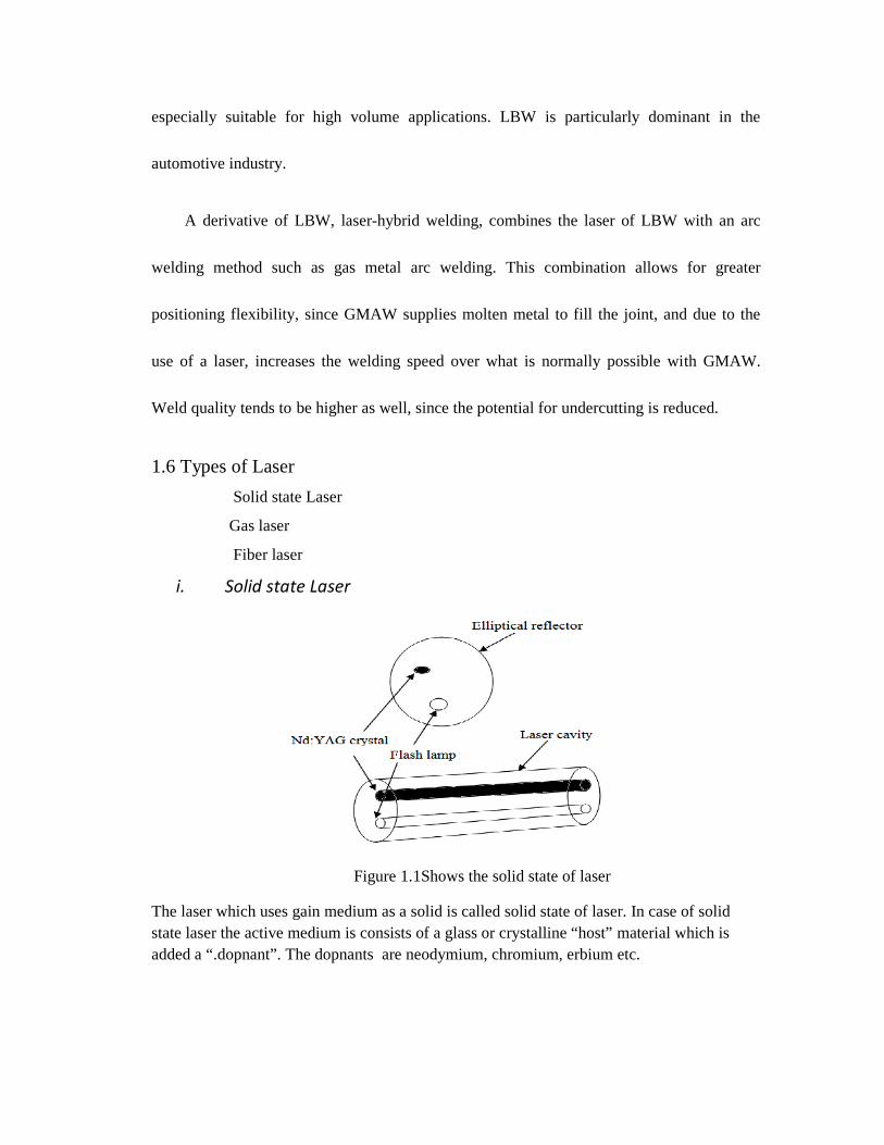
i. Solid state Laser

Figure 1.1Shows the solid state of laser

The laser which uses gain medium as a solid is called solid state of laser. In case of solidstate laser the active medium is consists of a glass or crystalline “host” material which isadded a “.dopnant”. The dopnants are neodymium, chromium, erbium etc.








1.6 Types of Laser

Solid state Laser

Gas laser

Fiber laser











1.6 Types of Laser

Solid state Laser

Gas laser

Fiber laser




A lot of media are present where the solid state laser can work. Butsome of are widely used these are Neodymium-doped yttrium aluminum garnet (Nd:YAG),

Neodymium-doped glass (Nd:glass), and Ytterbium-doped glass. These are mainly very highpower levels and having high energies also.

Ruby crystal is the first material used as lasers. Now aday’s also these ruby crystals are used in some cases. But these are not common because oftheir low efficiencies. In ambient or room temperature the ruby crystals emits short pulses oflight but at low temperature like cryogenic temperature, they can be prepared to emitcontinuous train of pulses.

ii. Gas laser

Figure1.2 Shows the Gas laser

In Gas laser an electric current is discharged through a gas to produce coherent light. The

first continuous light laser is the gas laser and the first laser to operate on the principle of

converting electrical energy to laser light. The first gas laser is the Helium-Neon (HeNe).

Advantages

• High volume of active material.

• Active material is relatively inexpensive.

• Almost impossible to damage the active material.

• Heat can be removed quickly from the cavity.

Applications

• He-Ne laser is mainly used in making holograms.

• In laser printing He-Ne laser is used as a source for writing on the photosensitive

material.

• He-Ne lasers were used in reading the Bar Code which is imprinted on the product.

They have been largely replaced by laser diodes.

• Ion lasers, mostly argon, are used in CW dye laser pumping

iii. Fiber laserIn case of fiber laser the active gain medium is the optical fiber. The gain

medium is doped with rare earth elements such as erbium,neodymium,

dysprosium,ytterbium etc. The rare earth elements are related to doped fiber

amplifications which provide light amplification without producing the laser

light.

Advantages and applications

The advantages of fiber lasers over other types include:

• Light is already coupled into a flexible fiber: The fact that the light is already in a

fiber allows it to be easily delivered to a movable focusing element. This is important

for laser cutting, welding, and folding of metals and polymers.

• High output power: Fiber lasers can have active regions several kilometers long, and

so can provide very high optical gain. They can support kilowatt levels of continuous

output power because of the fiber's high surface area to volume ratio, which allows

efficient cooling.

• High optical quality: The fiber's wave guiding properties reduce or eliminate thermal

distortion of the optical path, typically producing a diffraction-limited, high-quality

optical beam.

• Compact size: Fiber lasers are compact compared to rod or gas lasers of comparable

power, because the fiber can be bent and coiled to save space.

Fiber laser can also refer to the machine tool that includes the fiber resonator.

Applications of fiber lasers include material processing, telecommunications, spectroscopy,

and medicine

1.7 Nd: YAG Laser

The Nd: YAG laser is an optically pumped solid state laser system that is capable

of providing high power laser beam. The lasing medium is a colorless and isotropic

crystal Yttrium aluminum garnet (YAG: Y2Al5O12) having a four operational levels of

energy

Figure1.3 shows the Nd:YAG laser

The Commercial Nd: YAG lasers for welding applications are available from many

suppliers. According to the operation the laser is divided into three modes

1. Continuous output

2. Pulsed pumping

3. Q-switched mode

Continuous output of laser

According to the operating condition the laser is classified into two types i.e. continuous

mode and the pulsed mode. The power output is continuous over time or in the form of

pulse.

When the beam output power is constant over time, It is called continuous wave. Different

types of laser can be converted and operate in continuous wave mode. In case of continuous

wave operation it is necessary for the population inversion of the gain medium to be

continuously filled up again by a type of pump source which is steady state in nature.

Practically it is impossible for some lasing medium. In some cases of lasers it is required a

very high continuous power level which is practically not possible or destroy the laser by

producing excessive amount of heat.

Pulsed pumping

When the laser emission is not continuous then it is called pulse pumping. In pulse pumping

the optical power is looks like pulses. Some laser cannot produce in continuous mode they

only in the form of pulse. The pulse energy is equal to the ratio of ratio of average power to

the repetition rate. By lowering the rate of pulses we can increase the energy of pulse.

Q-switched mode

In Q-switching type due to the allowing of population inversion the loss in the resonator is

more than gain of the medium. This reduction is expressed by the quality factor ‘Q’. When

the pump energy is reaches about its maximum level the loss mechanism is suddenly

removed and the laser emission is started which shows the stored energy of the gain medium.

This type of energy is not continuous and it is pulse type with high pick power.

1.8 Principle of Laser Generation

The generation of a laser beam is essentially a three step process that occurs almost

instantaneously.

1. The pump source delivered energy to the medium, due to this energy the electrons are

excited and raised temporarily to the higher energy level. The electrons held in this excited

state cannot remains in this state for a long time and drop down to a lower energy level. In

this way, the electron looses their excess energy gained from the pump energy by emitting

the photon. This is called spontaneous emission and the photons produced by this method are

the seed for laser generation.

2. The photons emitted by spontaneous method strikes other electrons at the higher energy

levels state. When the Photon strikes the electron in the excited state to a lower energy level

another photon is produced. These two photons have same wave length and travelling with

same the same direction and this is called stimulated emission.

3. The photons are emitted in all directions, some of photons along the laser medium to

strike the resonator mirror and after striking in the mirror reflected back through the

medium. This resonator mirrors defines the preferential amplification direction of the

stimulated emission. For amplification there must be greater percentage of amplification

atom at the excited state in the lower energy level. This “population inversion” of more

atoms in the excited state leads to the conditions required for laser generation.

1.9 Material Selection

The laser can weld a wide range of metal i.e. steels nickels alloys, aluminum alloys, titanium

and copper.

Some materials are impossible for laser welding. As with other joining technology certain

types of material properties are specific to laser welding. These are

1. High thermal cycling effect.

2. Reflectivity of the material.

3. Vaporizing of volatile alloying elements.

Selection of material for welding purpose

1. The commonly used material for welding purpose is the steel.

2. The percentage of carbon is less than 0.12%

3. The Cr/Ni ratio for steel is greater than 1.7.

The nickel alloys and the titanium alloys can be welding easily. Copper can be welded in

some specific case.

1.10 Properties of YAG crystal

• The chemical Formula of YAG Crystal is Y3Al5O1

• The Molecular weight of Yag crystal 596.7

• The Crystal structure is Cubic in design.

• The Hardness is about 8–8.5 (Moh).

• Melting point of Yag crystal is 1950°C (3540 °)

• Density of YAG crystal is 4.55 g/cm3

1.11 Terminology

Peak power

Peak power is the direct power that can be selected by laser. It controls the maximum power

of each pulse. Units of peak power are watt(w)

Pulse width

Pulse width is the duration of laser in each pulse. This is also called on time in each pulse.

The units of pulse width is (ms).

Pulse energy

The pulse energy is the energy contained with each pulse. The product of pulse width and

the peak power gives the pulse energy i.e. E= peak power Х pulse width.

Pulse repetition rate

The pulse repetition rate is the number of pulse per second. The unit of pulse repetition rate

i.e. Hz

Average power

Average power is defined as the average power on number of pulse i.e. Average power is

equal to the product of pulse energy and the pulse repetition rate. The unit of average power

is watt (W)

Peak Power density

Peak power density is defined as the concentration of power at a certain area. Peak power

density is equal to the ratio of peak power to the spot area. The units of peak power density

are W/cm2

1.12 Advantages and disadvantages of laser beam welding

Advantages

1-Deep and narrow welds can be produced by the laser welding process.

2-Very less amount of distortion created by this type of welding .

3-In case of laser welding the heat affected area is less.

4-Excellent metallurgical quality is established by this welding process.

5- By this process very thinner components can be weld

6-Travel speed is more than other welding processes.

7-Laser beam welding is a non-contact welding process.

Disadvantages

1. In case of laser welding close fitting and well clamped joints are required. The small

focused spot size of a laser beam will pass through narrow gaps, especially between thin

sheets. Poorly fitting parts produce undercut welds without use of filler wire.

2. Laser welding required accurate beam/joint alignment .The narrow weld can easily miss

the joint line if not accurately positioned. The depth of beam focus is small and its position

about the work surface has to be accurately maintained to achieve the required power

density.

3. Precision work piece or beam manipulation equipment is necessary to control energy

input. The performance of manipulation equipment is also directly related to above.

4. Machine are work-shop based. Safety screening around the operating envelope of the laser

gun is essential for operator safety. This aspect is difficult to achieve for general on-side

welding operations. The optical stability of the laser resonator and system which transmits

the laser beam to the work is paramount for reliable welding performance. Therefore these

equipments need to be maintained on a stable base. The electrical and cooled water service

required to operate a laser, especially a high power CO2 laser are not readily portable.

5. Total equipment and operating costs are high in comparison with arc welding machines.

Lasers together with the necessary work handling and ancillary equipment are expensive to

purchase and operate. The required of high utilization to be cost effective. Careful adherence

to maintenance schedules is necessary to ensure high equipment up-times.

1.13 Objective of Work

Alloy 690 is the common material for heat exchangers in nuclear power plant industries.

Zircaloy-4 is used major percentage in nuclear spacer grids. Now also these are insufficient

for nuclear analysis. Titanium alloys are mainly used for aerospace engineering. These are

all high cost materials. These are all used in heat sensitive places. As the laser welding

method give higher efficiency, excellent controllability and the ability to focus laser

radiation in a small area producing a high intensity of heat force therefore laser welding is

mainly used in all these conditions. Joining of dissimilar metal is very difficult especially

when thermal conductivity of each is substantially different (example copper and steel).

For Simulation purpose ANSYS® is used, and the model used is the heat moving source

model. For simulation purpose the thermal properties like thermal conductivity, specific

heat and density of the metal is utilized. At the time of simulation thermal conductivity of

the material is taken as isotropic in nature. For structural simulation purpose the properties

like young’s modulus, poisons ratio, coefficient of thermal expansions are used. All the

values are collected from the previous works. These properties vary as a non linear function

of temperature. Considering the speed of the computer, storage space of memory in

simulation and due to computational constraints we simulate the one half of the model

because these are symmetry in nature.

CHAPTER

2

LITERATURE

REVIEW

2.1 Previous Work

Lee et al.[1] in the year 2010 using ANSYS® software of heat moving source model

found the temperature at different node. The material used by them was alloy 690 in butt

welding process. They observed that in LBW process the weldment has smaller HAZ and

narrower sensation region.

Sunar et al.[2] in the year of 2006 using FEM through the ANSYS® finite element

package showed the stress at the welding zone. The stress is maximum at the welding zone.

The temperature distribution in the transverse direction does not vary considerably, but

varies significantly in the longitudinal direction.

Zhao et al.[3] in the year 2011 using FEM found the temperature distribution of overlap

welding. The material used by them was Ti6Al4V and 42CrMo sheets. In their experiments

they used 1kW Nd:YAG laser material processing system with five-axis CNC working

station. The temperature field increase linearly with laser power at a constant scanning

velocity.

GuoMing et al.[4] in year 2007 using FEA software ANSYS® of traveling heat source

found the temperature at different node. In the experiment they used the stainless steel sheet.

On moving heat source the temperature distribution of work piece changes quickly with the

variety of time and space. Heating and cooling exists at the same time.

Wang et al. [5]in year 2011 using FLUENT software found the temperature distribution

on laser key hole welding. In this experiment stainless steel sheet of sized 5x3x1m3 was

used. The temperature at laser beam centre is much higher than the rest of the work piece.

The temperature gradients occur in the front vicinity of the keyhole.

Kong Fanrong and Kovacevic Radovan [6]in year 2010 using the ANSYS® code

observed penetration of laser beam. The numerical and experimental result shows that

penetration and width of the weld bead tend to increase with the decrease in the welding

speed. The numerical results show that a higher stress convergence exists at the HAZ of

weld and longitudinal stress (SZ) and transverse stress (SX) prevail in the hybrid welding

process.

Capriccioli Andrea and Frosi Paolo[7] in year 2009 using the ANSYS® FE model for

welding simulation. In experiments they used inconel 625 and AISI 316 for welding. The

temperature gradients increase with the speed. The thermal conductivity and specific heat

increase with the temperature.

Shanmugam et al.[8] in year 2012 using commercial FE code ANSYS® shows the

welding dimensions. They used 2.5mm thick AISI 304 austenitic steel sheet for laser spot

welding. The shape of welded spot is almost circular for a straight beam and it becomes

elliptical in nature as the beam is tilted from the vertical axis.

Sabbaghzadeh et al.[9] in year 2008 using the finite element code ANSYS® model

transient temperature profiles, the fusion dimensions and the heat affected zones. They used

steel 304 in their experiments. The absorptivity of the Nd:YAG laser radiation by the work

piece is clearly a complex function of a number of variables such as surface temperature,

beam power density, focal position of the laser beam relative to the work piece surface.

Zhu X.K. and Chao Y.J. [10]in year 2002 using the finite element welding simulation code

WELDSIM observed the temperature distribution, the residual stress and distortion. The

material used in the welding was 5052-H32 aluminum alloy having dimensions

12.2mmX6mmX6.25mm. The thermal conductivity has some effect on the distribution of

transient temperature field during welding. The yield stress is the key mechanical property in

welding simulation. Its value has significant effect on the residual stress and distribution.

Kazemi Komeil and Goldak John A.[11] In the year 2009 using parametric design

capabilities of the finite element code ANSYS® to simulate the laser full penetration

welding. The material used is AISI 304 steel. It was found that three of the most sensitive

parameters to the model in predicting weld shape are peclet number, the conductivity of the

material and absorption coefficient of material used for the circular disk source.

Turna et al.[12] in year 2011 using ANSYS® software simulate thermal and stress field in

welding tubes. The material used is austenitic stainless CrNi steel type AISI 304. The

Nd:YAG pulsed laser is used. Temperature and stress fields in the weld region were

computed by the finite element method.

Han et al.[13] in year 2012 resulted that the welding induced distortions are highly

dependent on geometry of the molten zone and the heat affected zone. They used Zircaloy-4

for their experiment. The welding induced distortions of thin sheets decrease as the laser

power is raised.

Martinson et al.[14] in the year 2009 using the ABAQUS® FE software for simulation of

residual stress developed in the different welding geometries. In the comparison of the

tangential residual stresses for RSW and LSW, LSW shows higher tensile residual stresses

inside the weld ring than those found in the nugget of RSW. The weld region in LSW has

been surrounded by a compressive region which is larger in magnitude than that of RSW.

Tsirkas et al.[15] in the year 2003 using SYSWELD FE code, which takes into account

thermal, metallurgical and mechanical aspects. The geometry examined was a butt- joint

specimen that consisted of the thick AH36 shipbuilding steel plates. Three dimensional finite

element models has been developed to simulate the laser welding processes and predict the

final distortions of a butt-joint specimen.

Yilbas et al.[16] in the year 2010 using XRD found the residual stress and by SEM change

in metallurgical effect in welding sites. The material used in the experiment is the mild steel.

The stress field developed is found by FEM, Residual stress developed is by XRD technique

and the morphological and metallurgical changes in the welding region are examined using

the optical microscopy and the SEM

Spina et al.[17] in the year 2007 using ABAQUS® thermal and mechanical analysis were

carried out. In the experiment they used aluminum alloys. The thermal loads induced by the

laser source at different welding speeds. The achievement is an efficient thermal modeling

of laser welding and its subsequent mechanical analysis.

Zain-ul-abdein et al.[18] in the year 2011 using the commercial finite element software

ABAQUS® and a FORTRAN programme encoding a conical heat source with Gaussian

volumetric distribution of flux. The material used for experiment is AA 6056. A comparison

between the experimental and simulation results shows a good agreement. Finally, the

residual stress and strain states in a T-joint are predicted.

Anawa E.M. and Olabi A.G.[19] in year 2008 using Taguchi approach in statistical

design of experiment (DOE) technique for optimizing the selected welding parameters in

terms of minimizing the fusion zone. In this experiment they used AISI 316 stainless-steel

and AIS 1009 low carbon steel plates of two different types. Laser power has strong effect

on fusion area. By changing the P value the response will be changed dramatically.

2.2 Motivation

From the above papers we come to know that a lot of work has been done on thermal

analysis and structural analysis using the laser power. Mainly they used steel, alloy 690,

titanium and aluminum for their purpose. Some people choose two dimensional model and

some people choose the three dimensional models. The temperature distribution is expressed

by three dimensional conduction equations. The temperature produced at the welding zone is

described by the Rosenthal equation. Two types of mesh is used to show the heat effected

zone and the temperature distribution of the metal. Maximum papers show that in laser

welding the heat affected zone is minimum. In case of laser welding the stress affected area

is also very low and comparatively to the far from the welding zone the stress is higher at the

welding zone side and it decreases towards the fixed side of the sheet. Very less amount

work has carried out of dissimilar metals like copper and steel because the conductivity of

the copper is much greater than other metal. Therefore in my project I choose dissimilar

metal like copper and steel. The properties are taken from the previous work.

CHAPTER

3

MODELINGAND

EXPERIMENTALANALYSIS

3.1Modeling

I. Theoretical modeling.

A Peclet number >10 is suited to a 2D model, and <10, to a 3D model. In our models, the

Peclet number is assumed to have a value of 81 for the GTAW process and 225 for the LBW

process. Thus, we adopt a 2D model. So, in constructing a theoretical model to predict the

thermal history of the HAZ during the welding process, the following [1]

Assumptions are made:

(1) The work piece material (Alloy 690) has an austenitic microstructure and undergoes

no phase transformation during the welding procedure.

(2) The thermal history of the HAZ is determined by the effects of conduction and

convection only, i.e. the effects of radiation are ignored. Moreover, the coefficient of

convection between the work piece and the environment is assumed to be a constant.

(3) Considering the speed of computer and storage space of memory in simulation, and

due to computational constraints, we simulated the one half models due to symmetry.

(4) The effects of the electric magnetic field in the GTAW process and the keyhole

phenomenon in the LBW process are neglected.

II. Mathematical modeling

The distribution of the temperature field induced during welding can be expressed by the

following energy balance equation:

ρC =∇( ∇ )- ρCU.∇Where ρ is the density ⁄ 3

C is the specific heat ⁄T is the temperature (k)

t is the time (s)

k is the thermal conductivity ⁄U is the welding velocity

G is the rate of heat generation or consumption per unit volume ( ⁄ 3)

In modeling the heat transmission during welding, the effects of weld pool stirring are

ignored. Moreover, k is assumed to be isotropic in all directions, the temperature gradient in

the depth direction of the work piece (i.e. ∂T/∂z) is supposed to be sufficiently small that it

can be neglected, and the heat flow is assumed to take place in two dimensions only. Thus,

the steady-state heat flow can be modeled using the following energy balance equation:[1]

ρC = k(T) { + }+ {( ) 2 +( )2}+ GIn the simplest scenario, the following assumptions are made:

1. The thermal conductivity k of the work piece is insensitive to changes in the temperature.

2. The only heat source acting on the work piece surface is that provided by the welding

source.

3. No heat is either produced or lost in any other region of the work piece. i. e.

G=q

The heat transmission during welding

=α { + }+ q

Where α is the thermal diffusivity of the work piece i.e. α= ⁄The temperature is produced by Rosenthal as

T (ζ, y, z) =T0+ exp (- ) k0 ( )

Where T0 = is the initial temperature of the of the work piece (k).

δ is the thickness of the work piece (m).

r= ( − ) +Construction of welding model

The sheets are placed on a stationary work plane with a fixed co-ordinate system i.e. ( x, y,

z)

The moving heat source is modeled using the moving co ordinate system ( ζ, y, z)

u= Moving heat source in the x-direction of the work plane at a constant velocity.

ζ=x- u. t

Initial and boundary condition

1. Initial condition

T(x, y, z, o) =T0 (x, y, z)

2. Boundary condition

{q}T . {η} =h f ( TB-TS),

Where {q}T is the heat flux field.

{ η}= unit outward normal vector.

H f is the film coefficient.

T B is the bulk temperature of the adjacent fluid.

T S is the temperature at the surface of the weldment .

In modeling the GTAW and LBW welding process, it is assumed that the electric arc or

the laser beam forms a disk-like shape on the surface of the weldment . The resulting

heat distribution is described by the following Gaussian function

q( x, ζ )= exp (- ) exp (- )

Q= Energy input rate (w)

c = characteristic radius of the heat flux distribution (m).

3.2 Experimental set up.

I. Materials.The raw materials selected for this experiment are copper and stainless

steel having thickness1mm. For thermal simulation purpose properties are used these

are thermal conductivity, specific heat, emissivity and density of the material. In

case of structural simulation the physical properties are used these are young’s

modulus, poisons ratio and the co-efficient of thermal expansion etc.

II. Properties of copper

Table no.3.1 shows the properties of copper at different temperatures. Thermal

conductivity and specific heats are changes with different temperature conditions.

Table number 3.1 shows the properties of copperTemp. (k) Density

(kg/m3)Young’smodulus(GPa)

Poisonsratio

Thermalconductivity(w/m.°k)

Specificheat(j/kg.°k)

293 8933 129.80 .34 400.68 383.48300 4001.00 385.00350 396.78 392.00373 395.20 394.73400 393.00 398.44450 389.93 403.00473 388.35 405.90500 386.50 408.00550 383.08 412.00573 381.50 414.80600 379.00 417.00650 376.23 421.00673 374.65 422.42700 372.80 425.00773 367.80 429.76800 366.00 432.00873 360.96 437.82900 359.11 441.001000 352.00 451.001073 347.26 460.071100 345.41 464.001200 339.00 480.001250 335.13 490.001300 331.71 506.00

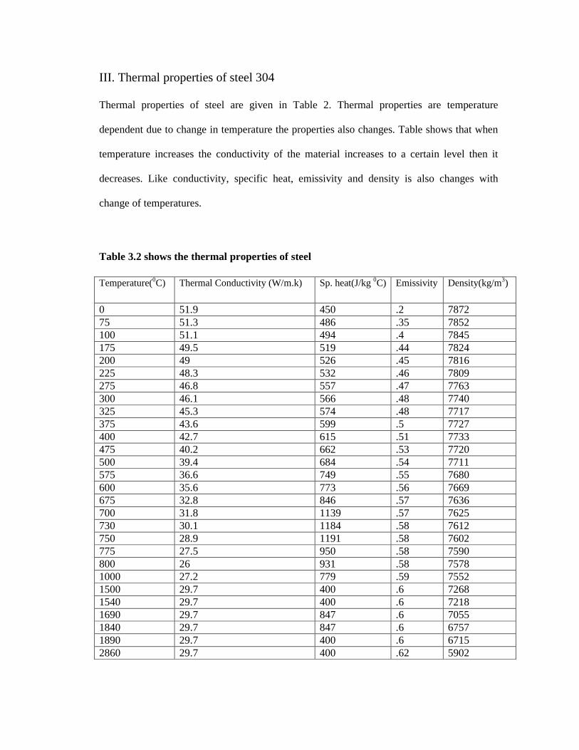
III. Thermal properties of steel 304

Thermal properties of steel are given in Table 2. Thermal properties are temperature

dependent due to change in temperature the properties also changes. Table shows that when

temperature increases the conductivity of the material increases to a certain level then it

decreases. Like conductivity, specific heat, emissivity and density is also changes with

change of temperatures.

Table 3.2 shows the thermal properties of steel

Temperature(0C) Thermal Conductivity (W/m.k) Sp. heat(J/kg 0C) Emissivity Density(kg/m3)

0 51.9 450 .2 787275 51.3 486 .35 7852100 51.1 494 .4 7845175 49.5 519 .44 7824200 49 526 .45 7816225 48.3 532 .46 7809275 46.8 557 .47 7763300 46.1 566 .48 7740325 45.3 574 .48 7717375 43.6 599 .5 7727400 42.7 615 .51 7733475 40.2 662 .53 7720500 39.4 684 .54 7711575 36.6 749 .55 7680600 35.6 773 .56 7669675 32.8 846 .57 7636700 31.8 1139 .57 7625730 30.1 1184 .58 7612750 28.9 1191 .58 7602775 27.5 950 .58 7590800 26 931 .58 75781000 27.2 779 .59 75521500 29.7 400 .6 72681540 29.7 400 .6 72181690 29.7 847 .6 70551840 29.7 847 .6 67571890 29.7 400 .6 67152860 29.7 400 .62 5902

3.3 Alpha Laser AL200

The Nd: YAG laser system has maximum power output of 200W. The pulse width is varies

from 0.5ms to 20ms. Maximum pulse energy is 9OJ and the laser spot size varies from .3to

2.2mm.

Figure 3.1Alpha laser AL 200

3.4 Laser parameters:

1. Average peak power (kW)

2. Pulse energy (J)

3. Pulse duration (ms)

4. Average peak power density (kW/m2)

5. Laser spot area (m2)

6. Mean laser power (kW)

7. Pulse frequency (in Hz)

3.5 Software

The software used in the CNC equipment was WIN Laser NC software (NC 4-

axis control)

Table 3.3 shows the specification of the laser equipment

TECHNICAL DATA AL 200 SPECIFICATIONS

LASER

Wavelength 1064 nm

Average power 200 W

Peak pulse power 9 KW

Pulse energy 150 mJ – 80 J

Pulse duration 0.5 ms – 20 ms

Pulse frequency Single pulse, 20Hz – 30 Hz

Welding spot diameter 0.3 mm – 2.2 mm

Pulse shaping Adjustable power-shaping within a laser

pulse

Control User-specific operation with up to 128

parameter sets

Focusing lens 150 mm

Viewing Optics Leica binocular with eyepieces for

spectacle users

POWER SUPPLY

Dimensions (L*W*H) 820*400*810 mm

Weight Approx 98 Kg

LASER BEAM SOURCE

With focusing unit (length *diameter) 1100*120 mm

Weight Approx 20 Kg

ELECTRICAL SUPPLY 3*400V / 3*16 A / 50-60 Hz / N, PE

COOLING Air cooled with internal cooling water-

circuit, no additional external cooling is

necessary.

3.6 Welding process

The mild steel and stainless steel plates to be welded were carefully placed such

that there was no gap between the edges to be welded. The alignment was ensured with

the help of the microscope provided in the laser apparatus. The plates were then welded

for a length of 25mm. This procedure is repeated for all the selected sets of parameters.

3.7 Grinding machine and Jig saw

Figure 3.2 shows the Grinding machine and Jig saw.

The grinding wheel composed of cutting particles called abrasive. The

grinding wheels made from matrix of coarse particles pressed and bonded together

to form sold of different shapes. The jigsaw is mainly for cutting purpose of the

sheet and the grinding wheel is used for finishing the edges of the sheet.

3.8 Simulation

For simulation purpose we take help or the software ANSYS®. First we choose the

element from the library for the simulation. After choosing the element we have to

apply the real constant values to the element and the thermal properties are added the

system. Dimensions are given according to the requirement of the practical applications.

After completing the modeling part meshing is started at the near finer mesh is used and

far from the weld bead course mesh is used. After the meshing operation the solution

operation is started. In solution part the initial condition is first added to the system,

mainly ambient temperature is taken as the initial temperature of the system. Then type

of heat transfer i.e. steady state or the transient condition is taken into consideration.

Then boundary condition is given to the system according to the data given in the

problem. In solution option some properties are added to the system. Then solution is

done by the ANSYS®. After the solution process the post processing part is started, in

post processing part it shows the results and also shows the graph of different condition.

In case of thermal modeling the post processing part shows the results I.e. the

temperature at different position by different colors. The values of temperature are also

given and these are given in different colors.

In case of structural analysis the physical properties are added to the system like young’s

modulus, poisons ratio, co-efficient of thermal expansion, etc. In thermo-physical

analysis the ambient temperature is taken as the initial condition. Thermo-physical

analysis both thermal and physical properties are added to the system. In this type of

analysis the stress field produced by the temperature, strain occurred due to temperature

rise can also be calculate.

3.9 Present Problem

For simulation purpose we take help or the software ANSYS®. The method is

chosen as the moving heat source type. For our simulation purpose we choose the 2-D

model. Then we choose the element type i.e.sheel-57. After choosing the element

applying the real constant values these are 0.004, 0.004, 0.004 and 0.004 . Thermal

conductivity of the steel is taken as 25 .⁄ , specific heat of steel 500 . ℃⁄ and

density of steel is taken as 7850 ⁄ . Then dimensions are taken as length equals to

0.025m and the breadth equals to 0.015m. Then in meshing we divide the length into 50

equal divisions and breadth into 30 equal divisions. After meshing we numbered all the

nodes using the “plot ctrls” menu. After completing the preprocessor work switch over to

the solution part.

In solution part first we choose type of heat transfer i.e. “transient type” then the initial

temperature i.e. 30°C is given to the system. Then scale of parameters is chosen i.e. taken

as DT equals to 0.1 and FL equals to 250. Heat flow of 155 ⁄ is given to the nodes

and all the time same amount of heat flow value is added to the nodes. Then using the

load step option we give the value of the end of load step, in this option we give the sub

step value equals to 5. The Ls file number is given as 1. After that we delete the heat

flow value from the node. Again same procedure is given to all the nodes. After given

the heat flow value to all the selected nodes and deleting the same from the nodes, delete

all load data option is chosen. Then solve option is given to the system through the Ls

files option. Ls File number is chosen, starting number is chosen as 1 and the ending

number is chosen as 5 and solution is over. In post processor option the contour plot is

drawn through the nodal solution and “dof of solution”. After that closing the node

numbers animation option is taken, in animation option the values are given as node

numbers equals to 5, time range is chosen from 0-0.5, auto contour scaling in ’off

condition then applying the “ok” option it shows the temperatures at different nodes.

From the above experiment and simulation we got the following results

CHAPTER

4

RESULTS

AND

DISCUSSION

41

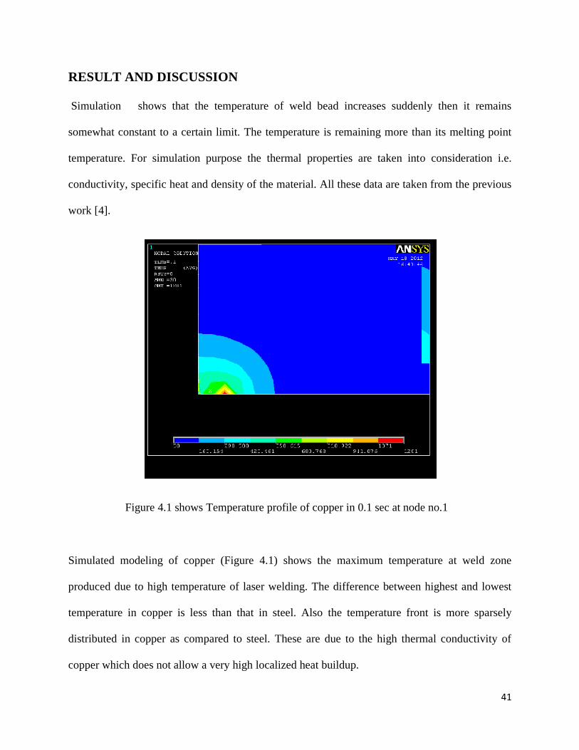
RESULT AND DISCUSSION

Simulation shows that the temperature of weld bead increases suddenly then it remains

somewhat constant to a certain limit. The temperature is remaining more than its melting point

temperature. For simulation purpose the thermal properties are taken into consideration i.e.

conductivity, specific heat and density of the material. All these data are taken from the previous

work [4].

Figure 4.1 shows Temperature profile of copper in 0.1 sec at node no.1

Simulated modeling of copper (Figure 4.1) shows the maximum temperature at weld zone

produced due to high temperature of laser welding. The difference between highest and lowest

temperature in copper is less than that in steel. Also the temperature front is more sparsely

distributed in copper as compared to steel. These are due to the high thermal conductivity of

copper which does not allow a very high localized heat buildup.

42

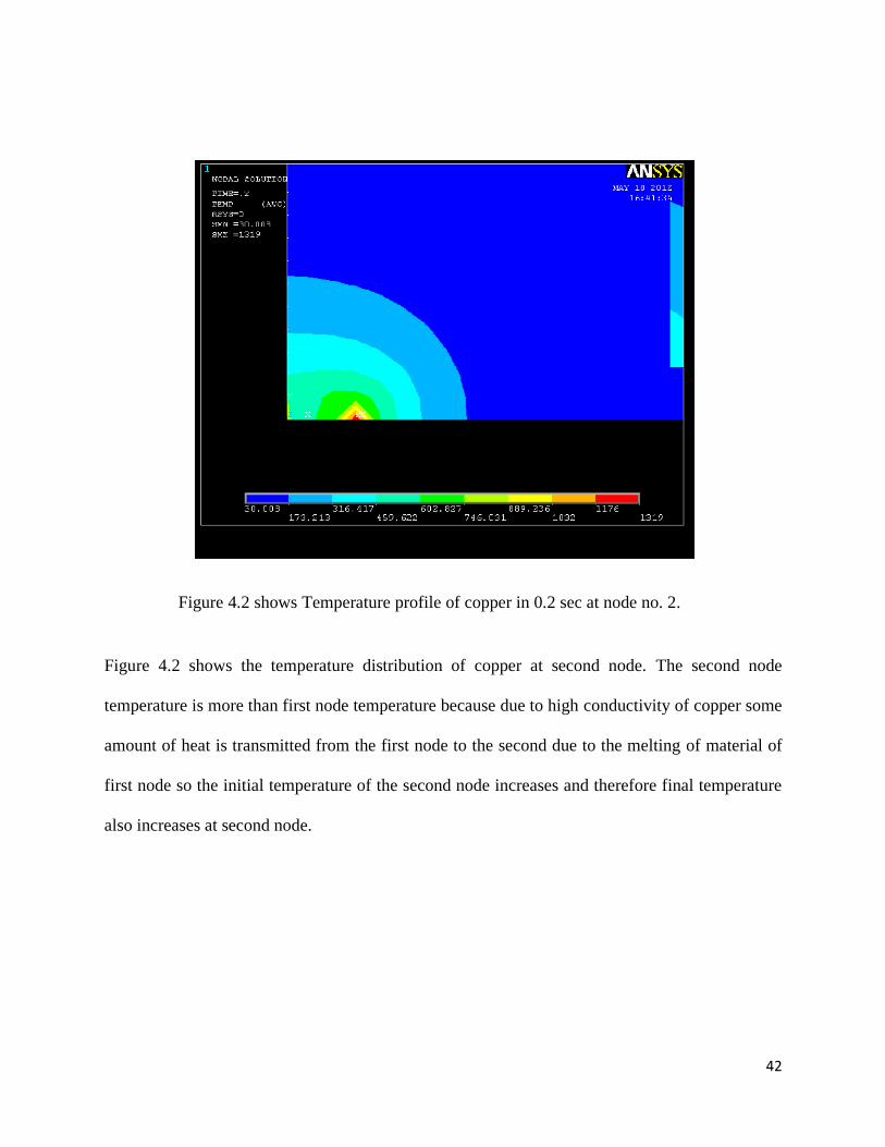
Figure 4.2 shows Temperature profile of copper in 0.2 sec at node no. 2.

Figure 4.2 shows the temperature distribution of copper at second node. The second node

temperature is more than first node temperature because due to high conductivity of copper some

amount of heat is transmitted from the first node to the second due to the melting of material of

first node so the initial temperature of the second node increases and therefore final temperature

also increases at second node.

43

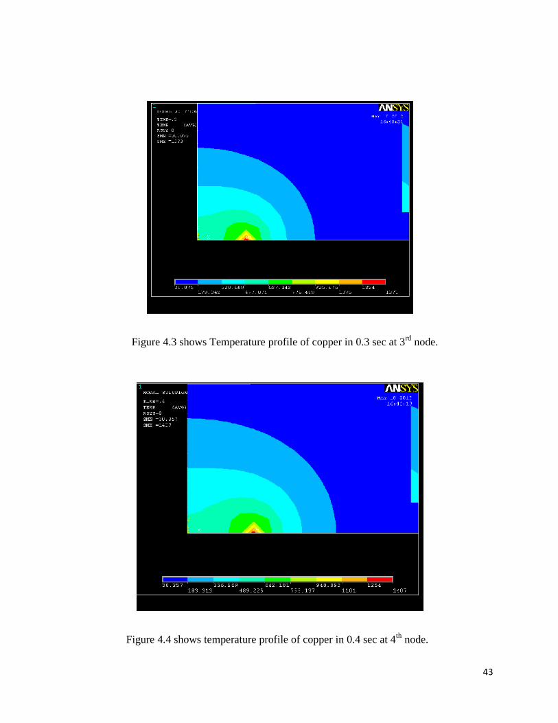
Figure 4.3 shows Temperature profile of copper in 0.3 sec at 3rd node.

Figure 4.4 shows temperature profile of copper in 0.4 sec at 4th node.

44

Figure 4.5 shows Temperature profile of copper in 0.5 sec at 5th node.

Figure 4.3, 4.4 and 4.5 shows the temperature profile of copper at 3rd, 4th and 5th nodes. Like the

second node the temperature of the 3rd, 4th and 5th node also increases but the rate of increase of

temperature is decrease. It shows that the rate of increase of temperature rises suddenly. It

happens because initially the 1st node is at the ambient condition, after touching the pulse to the

1st node it melts and the temperature of node 1 increases and due to conductivity of copper some

amount of heat is also transferred to the 2nd node and other node also in this way the initial

temperature of other nodes also increases and final temperature also increases.

45

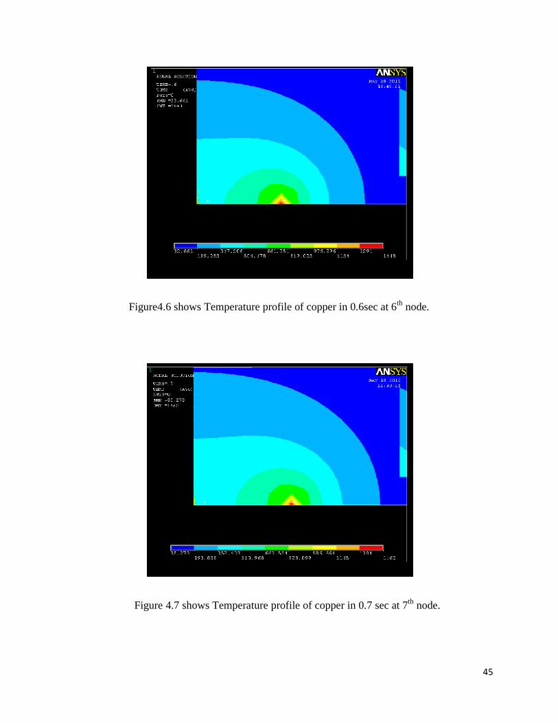
Figure4.6 shows Temperature profile of copper in 0.6sec at 6th node.


46


Figure4.9 shows Temperature profile of copper in 0.9 sec at 9th node.

47

Figure 4.10 shows Temperature profile of copper in 1sec at 10th node.

Figure 4.6, 4.7, 4.8, 4.9 and 4.10 shows the temperature profile of copper at 6th ,7th ,8th ,9th and

10th node. These figures show that the melting temperature remains constant at above nodes.

After some time it comes to the saturation state and the temperature does not increase further but

heat flow rate is added to the nodes. Due to the saturation state the initial temperature is remains

constant and the final temperature is also remains somehow constant. Which support the

practical assumptions .

48

0

200

400

600

800

1000

1200

1400

1600

1 2 3 4 5 6 7 8 9 10 11 12 13 14 15

Tem

pera

ture

°C

Node numbers

Figure4.11 shows the temperature at different nodes.

Figure 4.11 shows the melting point temperature of copper at different nodes. It shows that at

initially the melting temperature is rises suddenly then the rate of increase of temperature

decreases and it remains approximately constant. But the same amount of heat flow is added to

the system. After some time it comes to a saturation state due to this saturation state the initial

temperature is remains constant and therefore the final temperature is also remains constant.

49

Figure 4.12 shows temperature profile of steel in 0.1sec at 1st node.

Figure 4.12 shows the temperature distribution of steel. The simulation shows that the maximum

temperature is produced at welding zone and the same decreases while moving away from the

welding zone. The difference between the highest and the lowest temperature of steel is higher

than that in copper. Also the temperature front is less sparsely distributed in steel as compared to

copper. These are due to less thermal conductivity of steel than the copper.

50

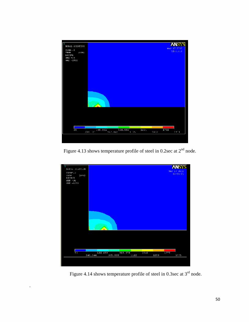
Figure 4.13 shows temperature profile of steel in 0.2sec at 2nd node.

Figure 4.14 shows temperature profile of steel in 0.3sec at 3rd node.

.

51

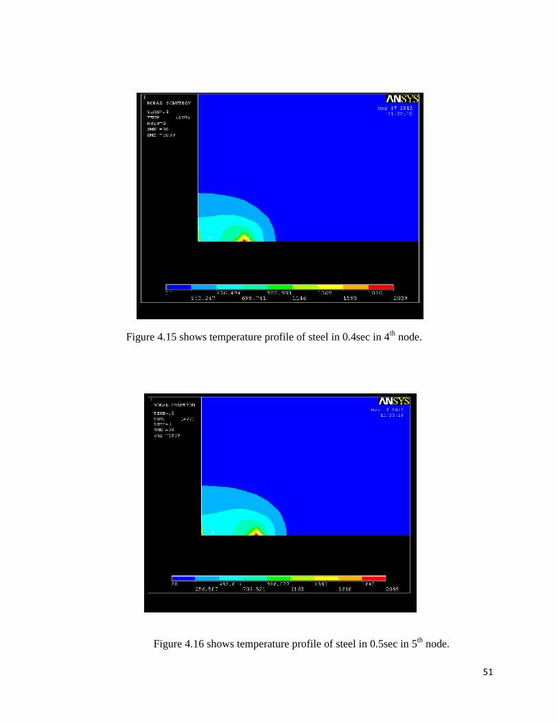
Figure 4.15 shows temperature profile of steel in 0.4sec in 4th node.

Figure 4.16 shows temperature profile of steel in 0.5sec in 5th node.

52

Figure 4.12, 4.13, 4.14, 4.15,and 4.16 shows the temperature profile of steel at 1st ,2nd

3rd ,4th and 5th nodes. It shows that the rate of increase of temperature rises suddenly. It happens

because initially the 1st node is at the ambient condition, after touching the pulse to the 1st node it

melts and the temperature of node 1 increases and due to conductivity of steel some amount of

heat is also transferred to the 2nd node and other node also in this way the initial temperature of

other nodes also increases and final temperature also increases.

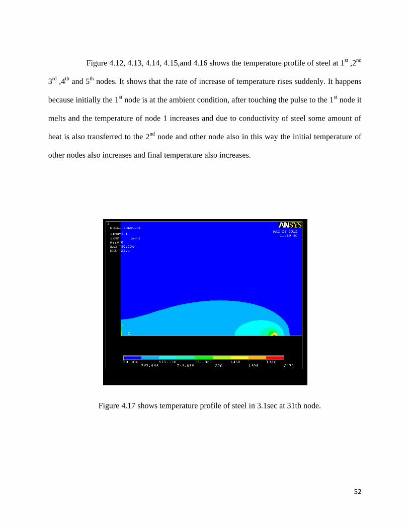
Figure 4.17 shows temperature profile of steel in 3.1sec at 31th node.

53

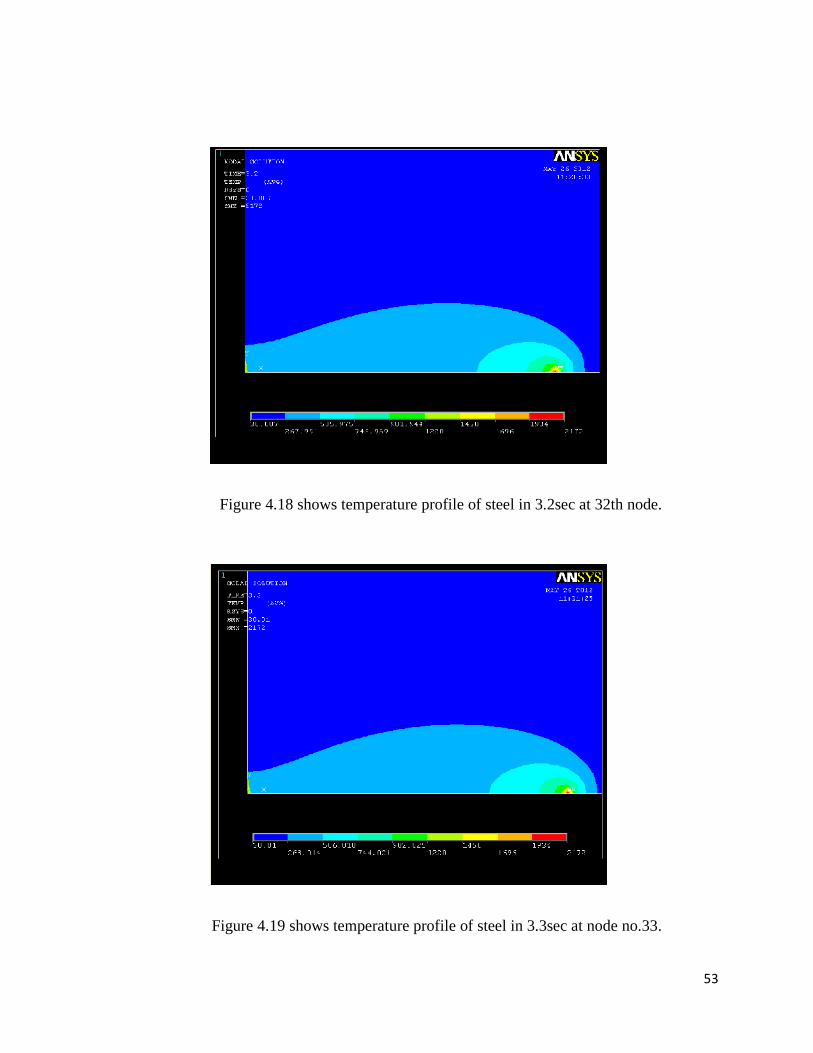
Figure 4.18 shows temperature profile of steel in 3.2sec at 32th node.

Figure 4.19 shows temperature profile of steel in 3.3sec at node no.33.

54

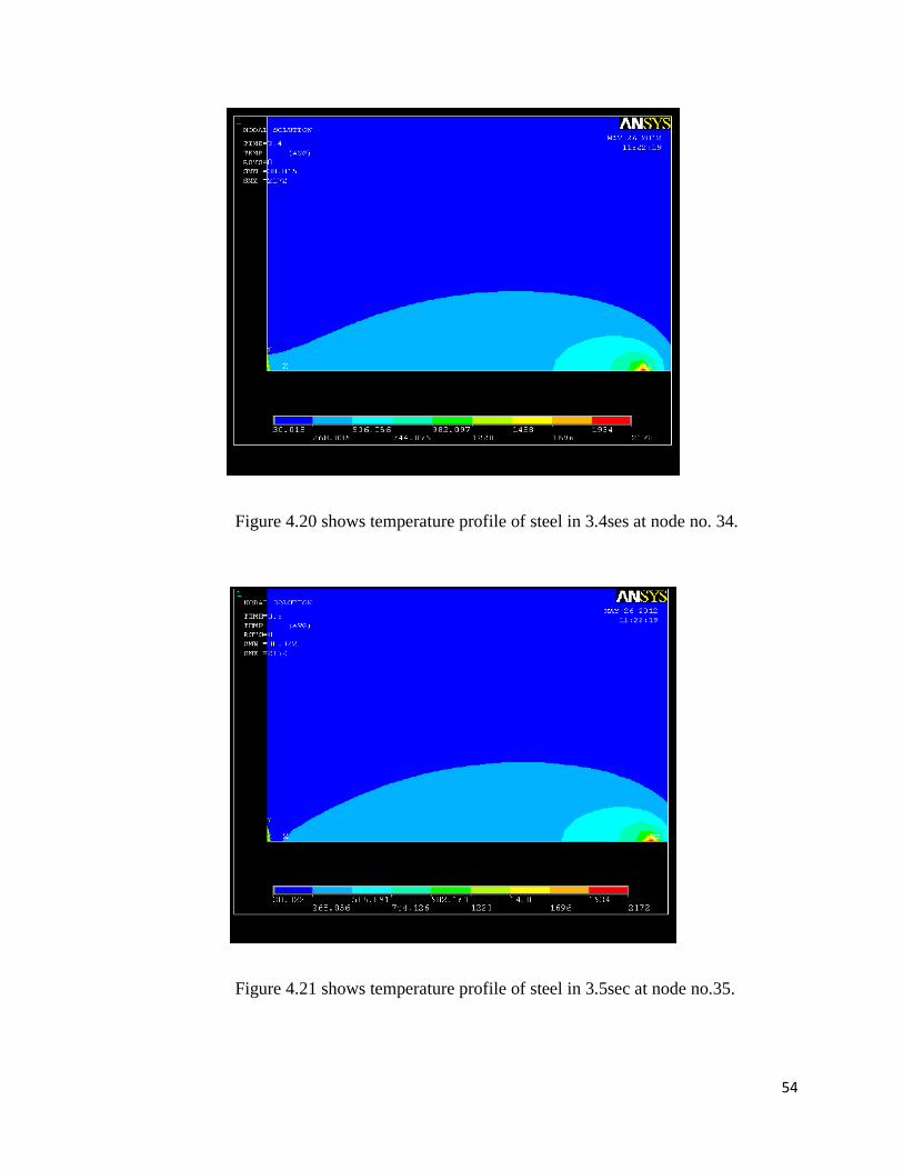
Figure 4.20 shows temperature profile of steel in 3.4ses at node no. 34.

Figure 4.21 shows temperature profile of steel in 3.5sec at node no.35.

55

Figure 4.17, 4.18, 4.19 ,4.20 and 4.21 shows the temperature profile of steel at 31th, 32th, 33th,

34th and 35th node. These figures show that the melting temperature remains constant at above

nodes. After some time it comes to the saturation state and the temperature does not increase

further but heat flow rate is added to the nodes. Due to the saturation state the initial temperature

is remains constant and the final temperature is also remains constant. Which support the

practical assumptions.

Figure 4.22 shows the temperature at different nodes.

Figure 33 shows the melting point temperature at different nodes. It shows that at initially the

temperature rises then it remains constant. At the initial condition the node is at the ambient

condition and after the welding started the temperature of the plate increases. Due to the thermal

conductivity property of the plate the heat is transferred to the other nodes and the initial

56

temperature of the plate increases and due to the increase of initial temperature the final

temperature is also increases because same amount of heat flow rate is added to the each node

After some time it comes to the saturation state and the initial temperature of the plate does not

increase further addition of heat flow rate. Therefore the final temperature also remains constant.

Which support the practical assumptions.

.

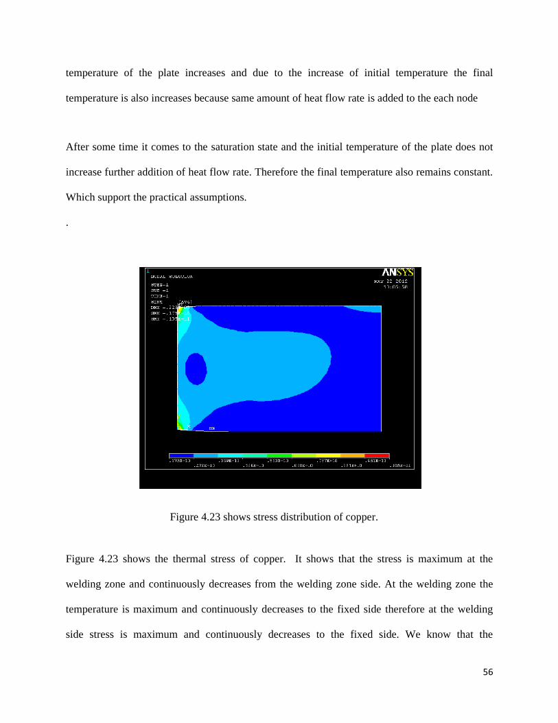
Figure 4.23 shows stress distribution of copper.

Figure 4.23 shows the thermal stress of copper. It shows that the stress is maximum at the

welding zone and continuously decreases from the welding zone side. At the welding zone the

temperature is maximum and continuously decreases to the fixed side therefore at the welding

side stress is maximum and continuously decreases to the fixed side. We know that the

57

conductivity of copper is more than steel so comparatively less amount of heat is produced at the

fusion zone of copper and therefore less stress is also produced.

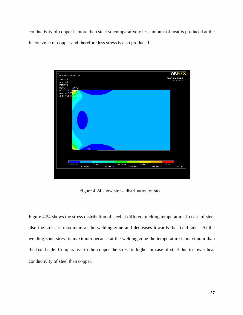
Figure 4.24 show stress distribution of steel

Figure 4.24 shows the stress distribution of steel at different melting temperature. In case of steel

also the stress is maximum at the welding zone and decreases towards the fixed side. At the

welding zone stress is maximum because at the welding zone the temperature is maximum than

the fixed side. Comparative to the copper the stress is higher in case of steel due to lower heat

conductivity of steel than copper.

58

1 4.2kW 1.9708mm 2 5.8kW 2.3356mm

3 5.1kW 2.134mm 4 5.2Kw 2.234mm

5 5.4kW 2.3112mm 6. 6.5kW 2.406

Figure 4.25 shows the weld diameter at different powers.

59

CHAPTER

5

CONCLUSIONS

60

From the above experimental work we deduced the following conclusions

1. The temperature of the welding bead increases rapidly at initial welding and achieve

steady state quickly in practical situation.

2. The thermal stress is decreases from the welding zone to the fixed side.

3. The diameter of the weld bead changes due to change in power keeping the other

parameters constant.

4. The heat affected zone is very small in case of laser welding.

5. Temperature distribution in thermal analysis mainly depends upon the thermal

properties like thermal conductivity, specific heat and density of the metal.

61

REFERENCES

62

1. Lee, H.T., Chen, C.T., Wu, J.L., 2010. Numerical and experimental investigation into effect of

temperature field on sensitization of Alloy 690 butt welds fabricated by gas tungsten arc welding

and laser beam welding. Journal of Material Processing Technology 210, 1636-1645.

2. Sunar,M.,Yilbas, B.S., Boran,K.,2006. Thermal and stress analysis of a sheet metal in

welding.Journal of Material Processing Technology 172,123-129.

3. Zhao,S., Yu,G., He,X., Zhang,Y., Ning,W.,2011. Numerical simulation and experimental

investigation of laser overlap welding of Ti6Al4V and 42CrMo. Journal of Material Processing

Technology 211, 530-537.

4. GuoMing,H., Jian,Z., JianQang,L., 2007.Dynamic simulation of the temperature field of stainless

steel laser welding. Material and design 28, 240-245.

5. Wang,R., Lei,Y., Shi,Yaowu., 2011.Numerical simulation of transient temperature field during

laser keyhole welding of 304 stainless steel sheet. Optics and Laser Technology 43,870-873.

6. Kong,F., Kovacevic,R., 2010.3D finite element modeling of the thermally induced residual stress

in the hybrid laser/arc welding of lap joint. Journal of Material Processing Technology 210,941-

950.

7. Capriccioli,A., Frosi,P., 2009. Multipurpose ANSYS FE procedure for welding processes

simulation. Fusion Engineering and Design 84, 546-553.

8. Shanmugam,N.S., Buvanashekaran,G., Sankaranarayanasamy,K., 2012. Some studies on weld

bead geometries for laser spot welding process using finite element analysis. Material and design

34, 412-426.

9. Sabbaghzadeh,J., Azizi,M., Torkamany,M.J., 2008 Numerical and experimental investigation of

seam welding with apulsed laser. Optics and Laser Technology 40, 289-296.

10. Zhu,X.K., Chao,Y.J.,2002 Effects of temperature-dependent material properties on welding

simulation. Computers and Structure 80, 967-976.

11. Kazmi,K., Goldak,J.A., 2009Numerical simulation of laser full penetration welding.

Computational Materials Science 44, 841-849.

63

12. Turna,M., Taraba,B., Ambroz,P., Sahul,M.,2011 Contribution to Numerical Simulation of Laser

Welding. Physics Procedia 12, 638-645.

13. Han,Q., Kim,D., Kim,D., Kim,N., 2012 Laser pulsed welding in thin sheets of Zircaloy-4. Journal

of Material Processing Technology212, 1116-1122.

14. Martinson,P.,Daneshpour,S., Kocak,M., Riekehr,S., Staron,P., 2009 Residual stress analysis

of laser spot welding of steel sheets. Material and Design 30,3351-3359.

15. Tsirkas,S.A., Papanikas,P., Kermanidis,T, 2003 Numerical simulation of the laser

welding process in butt-joint specimens. Journal of Material Processing Technology 134,59-

69.

16. Yilbas,B.S., Arif,A.F.M., Abdul Aleem,B.J., 2010 Laser welding of low carbon steel and

thermal stress analysis.Optics & Laser Technology 42 ,760–768.

17. Spina,R., Tricarico,L., Basile,G., Sibillano,T., 2007 Thermo-mechanical modeling of

laser welding of AA5083 sheets. Journal of Material Processing Technology 191,215-219.

18. Zain-ul-abdein, M.,Nelias,D., Tullien,J.,Boitout,F., Dischert,L., Noe,X., 2011 Finite

element analysis of metallurgical phase transformations in AA 6056-T4 and their effects

upon the residual stress and distortion states of a laser welded T-joint. International

Journal of Pressure Vessels and Piping 88,45-56.

19. Anawa,E.M., Olabi,A.G.,2008 Using Taguchi method to optimize welding pool of

dissimilar laser-welded components. Optics & Laser Technology 40 , 379–388

DYNAMIC SIMULATION OF TEMPERATURE FIELD IN Nd:YAG …ethesis.nitrkl.ac.in/4037/1/210ME3145.pdf(i...

Documents

Transcript of DYNAMIC SIMULATION OF TEMPERATURE FIELD IN Nd:YAG …ethesis.nitrkl.ac.in/4037/1/210ME3145.pdf(i...