Dynamic Reserve Prices for Repeated Auctions: Learning ...yk2577/dynamic_reserve.pdf · Dynamic...

Dynamic Reserve Prices for Repeated Auctions:

Learning from Bids

Yash Kanoria

Graduate School of Business, Columbia University

[email protected]

Hamid Nazerzadeh

Marshall School of Business, University of Southern California

[email protected]

A large fraction of online advertisements are sold via repeated second price auctions. In these auctions, the

reserve price is the main tool for the auctioneer to boost revenues. In this work, we investigate the following

question: Can changing the reserve prices based on the previous bids improve the revenue of the auction,

taking into account the long-term incentives and strategic behavior of the bidders? We show that if the

distribution of the valuations is known and satisfies the standard regularity assumptions, then the optimal

mechanism has a constant reserve. However, when there is uncertainty in the distribution of the valuations

and competition among the bidders, previous bids can be used to learn the distribution of the valuations and

to update the reserve prices. We present a simple approximately incentive-compatible and optimal dynamic

reserve mechanism that can significantly improve the revenue over the best static reserve in such settings.

1. Introduction

Advertising is the main component of the monetization strategy of most Internet companies. A large

fraction of online advertisements are sold via advertisement exchange platforms such as Google’s

Doubleclick (AdX) and Yahoo!’s Right Media.1 Using these platforms, online publishers such as

the New York Times and the Wall Street Journal sell the advertisement space on their webpages

to advertisers. A large fraction of advertisement space is allocated using auctions where advertisers

bid in real time for a chance to show their ads to the users. Every day, tens of billions of online ads

are sold via these exchanges (Muthukrishnan 2009, McAfee 2011, Balseiro et al. 2011, Celis et al.

2014).

The second-price auction is the dominant mechanism used by the advertisement exchanges.

Among the reasons for such prevalence are the simplicity of the second-price auction and the fact

1 Other examples of major ad exchanges include Rubicon, AppNexus, and OpenX.

1

Kanoria and Nazerzadeh: Dynamic Reserve Prices for Repeated Auctions

2 00(0), pp. 000–000, c© 0000 INFORMS

that it incentivizes the advertisers to be truthful. The second price auction maximizes the social

welfare (i.e., the value created in the system) by allocating the item to the highest bidder.

In order to maximize the revenue in a second price auction, the auctioneer can set a reserve

price and not make any allocations when the bids are low. In fact, under symmetry and regularity

assumptions (see Section 2), the second-price auction with an appropriately chosen reserve price

is optimal and maximizes the revenue among all selling mechanisms (Myerson 1981, Riley and

Samuelson 1981).

However, in order to set the reserve price effectively, the auctioneer requires information about

distribution of the valuations of the bidders. A natural idea, which is widely used in practice, is to

construct these distributions using the history of the bids. This approach, though intuitive, raises

a major concern with regards to long-term (dynamic) incentives of the advertisers. Because the

bid of an advertiser may determine the price he or she pays in future auctions, this approach may

result in the advertisers shading their bids and ultimately in a loss of revenue for the auctioneer.

To understand the effects of changing reserve prices based on the previous bids, we study a

setting where the auctioneer sells impressions (advertisements space) via repeated second price

auctions. We demonstrate that the long-term incentives of advertisers play an important role in the

performance of these repeated auctions by showing that under standard symmetry and regularity

assumptions (i.e., when the valuations are drawn independently and identically from a regular

distribution), the optimal mechanism is running a second price auction with a constant reserve

and changing the reserve prices over time is not beneficial. However, when there is uncertainty in

the distribution of the valuations and competition among the bidders, we show that there can be

substantial benefit in learning the reserve prices using the previous bids.

More precisely, we consider an auctioneer selling multiple copies of an item sequentially. The

item is either a high type or a low type. The type determines the distribution of the valuations

of the bidders. The type of the item is not a-priori known to the auctioneer. Broadly, we show

the following: when there is competition between bidders and the valuation distributions for the

two types are sufficiently different from each other, there is a simple dynamic reserve mechanism

that can effectively “learn” the type of the item, and thereafter choose the optimal reserve for

that type.2 As a consequence, the dynamic reserve mechanism does much better than the best

fixed reserve mechanism, and in fact, achieves near optimal revenue. Importantly, the mechanism

retains (approximate) incentive compatibility; implying that bidders cannot gain significantly by

deviating from truthfulness; see Section 2.

2 On the other hand, when the valuation distributions for the two types are close to each other, the improvement

from changing the reserve is insignificant.


00(0), pp. 000–000, c© 0000 INFORMS 3

We obtain our results using a simple mechanism called the threshold mechanism. In each round,

the mechanism implements a second price auction with reserve. The reserve price starts at some

value, and stays there until there is a bid exceeding a pre-decided threshold, after which the reserve

rises (permanently) to a higher value. We also present a generalization of this mechanism where

the reserve rises when sufficiently many bidders bid above the threshold.

We compare the revenue of our mechanism with two benchmarks. Our baseline is the static

second price auction with the optimal constant reserve. Our upper-bound benchmark is the opti-

mal mechanism that knows the type of the impressions (e.g., high or low) in advance. These two

benchmarks are typically well separated. We show that the threshold mechanism is near optimal

and obtains revenue close to the upper-bound benchmark. In addition, we present numerical illus-

trations of our results that show up to 23% increase in revenue by our mechanism compared with

the static second price auctions. These examples demonstrate the effectiveness of dynamic reserve

prices under fairly broad assumptions.

Related Work

In this section, we briefly discuss the closest work to ours in the literature along different dimensions

starting with the application in online advertising.

Ostrovsky and Schwarz (2009) conducted a large-scale field experiment at Yahoo! and showed

that choosing reserve prices, guided by the theory of optimal auctions, can significantly increase

the revenue of sponsored search auctions. To mitigate the aforementioned incentive concerns, they

dropped the highest bid from each auction when estimating the distribution of the valuations.

However, they do not formally discuss the consequence of this approach.

Another common solution offered to mitigate the incentive constraints is to bundle different

types of impressions (or keywords) together so that the bid of each advertiser would have small

impact on the aggregate distribution learned from the history of bids. However, this approach may

lead to significant estimation errors, resulting in a sub-optimal choice of reserve price.

Recently, Cesa-Bianchi et al. (2013), Mohri and Medina (2014b) study the problem of learning

optimal reserve prices for repeated second-price auctions but they ignore the strategic aspects and

incentive compatibility issues. To the extent of our knowledge, ours is the first work that rigorously

studies the long-term and dynamic incentive issues in repeated auctions with dynamic reserves.

Iyer et al. (2011) and Balseiro et al. (2013) demonstrate the importance of setting reserve prices

in dynamic setting in environments where agents are uncertain about their own valuations, and

respectively, are budget-constrained. We discuss the methodology of these papers in more details

at the end of Section 7. McAfee et al. (1989), McAfee and Vincent (1992) determine reserve prices

in common value settings.


4 00(0), pp. 000–000, c© 0000 INFORMS

Our work is closely related to the literature on behavior-based pricing strategies where the seller

changes the prices for a buyer (or a segment of the buyers) based on her previous behavior; for

instance, increasing the price after a purchase or reducing the price in the case of no-purchase;

see Fudenberg and Villas-Boas (2007), Esteves (2009) for surveys.

The common insight from the literature is that the optimal pricing strategy is to commit to a

single price over the length of the horizon (Stokey 1979, Salant 1989, Hart and Tirole 1988). In fact,

when customers anticipate reduction in the future prices, dynamic pricing may hurt the seller’s

revenue (Taylor 2004, Villas-Boas 2004). Similar insights are obtained in environments where the

goal is to sell a fixed initial inventory of products to unit-demand buyers who arrive over time (Aviv

and Pazgal 2008, Dasu and Tong 2010, Aviv et al. 2013, Correa et al. 2013).

There has been renewed interest in behavior-based pricing strategies, mainly motivated by the

development in e-commerce technologies that enables online retailers and other Internet companies

to determine the price for the buyer based on her previous purchases. Acquisti and Varian (2005)

show that when a sufficient proportion of customers are myopic or when the valuations of customers

increases (by providing enhanced services) dynamic pricing may increase the revenue. Another

setting where dynamic pricing could boost the revenue is when the seller is more patient than

the buyer and discounts his utility over time at a lower rate than the buyer (Bikhchandani and

McCardle 2012, Amin et al. 2013, Mohri and Medina 2014a). See Taylor (2004), Conitzer et al.

(2012) for privacy issues and anonymization approaches in this context. In contrast with these

works, our focus is on auction environments and we study the role of competition among strategic

bidders.

The problem of learning the distribution of the valuation and optimal pricing also have been

studied in the context of revenue management and pricing for markets where each (infinitesimal)

buyer does not have an effect on the future prices and demand curve can be learned with near-

optimal regret (Segal 2003, Besbes and Zeevi 2009, Harrison et al. 2012, Wang et al. 2014); see den

Boer (2014) for a survey. In this work, we consider a setting where the goal is to learn the optimal

reserve price with (finitely many) strategic and forward-looking buyers, with multi-unit demand,

where the action of each buyer can change the prices in the future.

Organization. The rest of the paper is organized as follows. We formally present our model

in Section 2, followed by our lower bound and upper bound revenue benchmarks in Section 3. We

describe the threshold mechanism in Section 4. We show that the mechanism is dynamic incentive

compatible in Section 5. In Sections 6, we present an extension of the threshold mechanism. We

provide a discussion in Section 7 and conclude in Section 8.


00(0), pp. 000–000, c© 0000 INFORMS 5

2. Model and Preliminaries

A seller auctions off T > 1 items to n≥ 1 agents in T rounds of second price auctions, numbered

t= 1,2, . . . , T . The items are of type high or low denoted by s∈ L,H, where informally we think

of an item of type H as being more valuable than an item of type L. The items are all of the same

type. The type is s with probability ps.

The valuation of agent i∈ 1, . . . , n for an item of type s, denoted by vi, is drawn independently

and identically from distribution Fs, i.e., the valuations are i.i.d. conditioned on s. Note that agents’

valuations are identical in each round (if they participate, see below). In Section 7 we consider an

extension of our model where the valuations of the agents may change over time.

Each agent participates in each auction with probability αi exogenously and independently across

rounds and agents. One can think of αi’s as throttling probabilities3 or matching probabilities to

a specific user demographic (Celis et al. 2014). Let Xit be the indicator random variable corre-

sponding to the participation of agent i in auction at time t. Note that αi = E[Xit]. We denote

the realization of Xit by xit. Agent i learns xit at the beginning of round t. 4 In particular, our

(incentive compatibility) results hold in the special case when all the agents participate in all the

auctions, i.e., αi = 1 for all i. Participation probabilities allow us to model (ad exchange) auctions

in which a small number of bidders participate in each auction (cf. Celis et al. (2014)).5

Information Structure. We assume T , pL, and pH to be common knowledge. We also assume

that the type of the item s is unknown to the auctioneer, who only knows ps, and this is common

knowledge. In our motivating application, advertisers sometimes may have more information about

the value of a user or an impression than the publisher. Thus, we allow for both possibilities:

• the type of the item s is unknown to the agents, only ps is common knowledge among the

agents and seller; or,

• the type of the item s is common knowledge among the agents.

We prove our results for the latter information structure since it corresponds to a stronger require-

ment for the incentive compatibility of the mechanism; hence, our results remain valid in the former

information structure, i.e., agents have the same information as the seller about the type of the

3 Due to budget and bandwidth constraints or other considerations, online advertising platforms often randomly

select a subset of bidders, from all eligible advertisers, to participate in the auction. This process is referred to as

throttling (Goel et al. 2010, Charles et al. 2013, Chakraborty et al. 2010).

4 In our setting, the population of the agents is fixed over time; see Said (2011), Vulcano et al. (2002) for sequential

second price auctions with randomly arriving buyers.

5 Thus, the expected number of bidders participating in each auction is∑i αi, which may be much smaller than n,

for instance, in Example 1, we have∑i αi = 1 whereas n= 20.


6 00(0), pp. 000–000, c© 0000 INFORMS

item. Similarly, we assume that αi’s are common knowledge among the agents and the auction-

eer. Our mechanism remains incentive compatible, as defined below, if the agents have incomplete

information about the αi’s. At the start, each agent i knows his own valuation, vi, but not the

other agents’ valuations (but agents may make inferences about the valuations of the other agents

over time).

Let us now consider the seller’s problem. The seller aims to maximize her expected revenue via

a repeated second price auction.

A “generic” dynamic second price mechanism. At time 0, the auctioneer announces the

reserve price function Ω :H→R+ that maps the history observed by the mechanism to a reserve

price. The history observed by the mechanism up to time τ , denoted by HΩ,τ ∈H, consists of, for

each round t < τ , the reserve price, the agents participating in round t and their bids, and the

allocation and payments at that round. More precisely,

HΩ,τ = 〈(r1, x1, b1, q1, p1), · · · , (rτ−1, xτ−1, bτ−1, qτ−1, pτ−1)〉

where

• rt is the reserve price at time t.

• xt = 〈x1t, · · · , xnt〉. Here xit is equal to 1 if agent i participates in the auction for item t.

• bt = 〈b1t, · · · , bnt〉 where bit denotes the bid of agent i at time t. We assign bit = φ if xit = 0,

i.e., if agent i does not participate in round t.

• qt corresponds to the allocation vector. Since the items are allocated via the second price

auction with reserve rt, if all the bids are smaller than rt, the item is not allocated. Otherwise, the

item is allocated uniformly at random to an agent i? ∈ arg maxibit and we have qi?t = 1. For all

the agents that did not receive the item, qit is equal to 0.

• pt is the vector of payments. If qit = 0, then pit = 0 and if qit = 1, then pit =

maxmaxj 6=i bjt , rt.

Note that in our notation, Ω includes a reserve price function for each t= 1,2, . . . , T . The length

of the history H implicitly specifies the round for which the reserve is to be computed. Further

note that the auctioneer commits beforehand to a reserve update rule Ω (cf. Devanur et al. (2014)).

An important special case is a static mechanism where the reserve is not a function of the

previous bids and allocations.

We can now define the seller problem more formally. The seller chooses a reserve price function

Ω that maximizes the expected revenue, which is equal to E[∑T

t=1

∑n

i=1 pit

], when the buyers play

an equilibrium with respect to the choice of Ω. In order to define the utility of the agents, let Hik


00(0), pp. 000–000, c© 0000 INFORMS 7

denote the history observed by agent i up to time t including the allocation and payments of (only)

agent i. Namely,

Hik = 〈(r1, xi,1, bi,1, qi,1, pi,1), · · · , (rt−1, xi,t−1, bi,t−1, qi,t−1, pi,t−1)〉.

Bidding strategy Bi : R×Hi ×R→ R of agent i maps the valuation of the agent vi, history Hit,

and the reserve rt at time t to a bid bit = Bi(vi,Hit, rt). Here Hi is the set of possible histories

observed by agent i. 6

Definition 1 (Best-Response) Given strategy profile <B1,B2, · · · ,Bn >, Bi is a best-response

strategy to the strategy of other agents B−i, if, for all s and vi in the support of Fs, it maximizes

the expected utility of agent i,

Ui(vi, s,Bi,B−i) = E

[T∑t=1

viqit− pit

],

where the expectation is over the valuations of other agents, the participation variables xjt’s, and

any randomization in bidding strategies. Strategy Bi is an ε-best-response if, for all vi in the

support,

Ui(vi, s,Bi,B−i)≥Ui(vi, s,BR(vi, s,B−i),B−i) +Tαiε ,

where BR denotes a best response.

Note that αiT is the expected number of rounds in which agent i participates. Therefore, under an

ε-best-response, on average the agent loses at most ε in utility, relative to playing a best response,

per-round of participation.

A mechanism is incentive compatible if, for each agent i, the truthful strategy is a best-response

to the other agents being truthful. In this paper, we consider the notion of approximate incentive

compatibility and assume that an agent does not deviate from the truthful strategy when the

benefit from such a deviation is insignificant. This notion is appealing when characterizing, or

computing, the best response strategy is challenging (Archer et al. 2004, McSherry and Talwar

2007, Nazerzadeh et al. 2013).7 In online ad auctions, finding profitable deviation strategies requires

6 Similar to the common practice in ad exchanges, we assume that agents see the reserve price before they bid. Note

that, similar to s and αi’s, our incentive compatibility results are still valid if the agents have incomplete information

about previous and current reserve prices.

7 Approximate incentive compatibility correspond to a special case of approximate Nash equilibrium (Daskalakis et al.

2009, Chien and Sinclair 2011, Kearns and Mansour 2002, Feder et al. 2007, Hemon et al. 2008)) where the focus is

on the truthful strategy. In Section 7, we provide a comparison with the notion of mean-field equilibrium (Iyer et al.

2011, Balseiro et al. 2013, Gummadi et al. 2013).


8 00(0), pp. 000–000, c© 0000 INFORMS

solving complicated dynamic programs in a highly uncertain environment, so agents can plausibly

be expected to bid truthfully under an approximately incentive compatible mechanism.

Definition 2 (Approximate Incentive Compatibility) A mechanism is ε-incentive compati-

ble if the truthful strategy of agent i is an ε-best-response to the truthful strategy of other agents

for all s and all vi in the support of Fs.

In Section 5 (Definition 3) we present a stronger and dynamic notion of incentive compatibility

that implies that with probability close to 1, truthfulness remains an ε-best-response for the agents

over time. We also provide conditions under which our proposed mechanism satisfies this stronger

notion.

3. Benchmarks

In this section we introduce suitable lower and upper-bound revenue benchmarks for mechanism

design in our setting.

To obtain a lower bound on revenue we consider the static mechanism, which implements a

second price auction in each round with a constant reserve r0. The reserve is chosen at time 0

before the mechanism observes any of the bids, and does not change over time.8 The reserve r0 is

chosen optimally based on the prior information available to the auctioneer.

For an upper-bound on revenue, we consider the optimal T -round mechanism that knows the

type of the items (this is a “genie-aided” setting where a genie reveals s to the auctioneer). The

benefit from doing this is two-fold: First, we avoid the intractable problem of finding the optimal

T -round mechanism with s unknown.9 Second, the optimal mechanism in the genie-aided setting

turns out to be have a simple and revealing structure that later facilitates our construction of the

“threshold mechanism” that achieves revenue close to the upper bound benchmark even without

knowing s beforehand.

Throughout this paper, we make the following standard regularity assumption (cf. Myerson

(1981)).

8 Since the valuations of the agents are correlated through the type of the items, finding the optimal static auction

is challenging and could be computationally intractable (Papadimitriou and Pierrakos 2011). Cremer and McLean

(1988) proposed a mechanism that can extract the whole surplus if the valuations are correlated by offering lotteries

to the bidders; however, their mechanism is significantly different from practically used mechanisms in online ad

auctions; furthermore, their mechanism is not ex-post individually rational which is a desirable property satisfied by

the second price auction; also see Fu et al. (2014).

9 In fact, the optimal single round mechanism is itself intractable. See footnote 8.


00(0), pp. 000–000, c© 0000 INFORMS 9

Assumption 1 (Regularity) Distribution Fs, for s ∈ L,H, with density fs, is regular, i.e.,

c.d.f. Fs(v) and(v− 1−Fs(v)

fs(v)

)are strictly increasing in v over the support of Fs.

Examples of regular distributions include many common distributions such as the uniform, Gaus-

sian, log-normal, etc.

If s is known and Fs is regular, then, we know from Myerson (1981) that the optimal mechanism

for T = 1 is the second price auction with reserve price r?s that is the unique solution of

r− 1−Fs(r)fs(r)

= 0 . (1)

We generalize this result to T rounds.

Proposition 1 (No “dynamic” improvement with single type) If the valuations are drawn

i.i.d. from a regular distribution (i.e., s is known and Fs satisfies Assumption 1), the optimal

mechanism is the second price auction with a constant reserve that is the solution of Eq. (1) and

there is no benefit from having dynamic reserve prices.

Proposition 1 says that even for T > 1, the revenue maximizing mechanism simply runs T second

price auctions with a constant reserve of r?s , obtaining an expected revenue that is T times the

revenue of a single Myerson auction. We call this the upper-bound revenue benchmark.

We prove Proposition 1 in the appendix using a reduction argument that reduces a mechanism

in the T -round setting to a mechanism for a single-round. The proposition generalizes the insights

from settings with a single buyer (Stokey 1979, Baron and Besanko 1984, Salant 1989, Hart and

Tirole 1988, Acquisti and Varian 2005) to auction environments with multiple buyers.

An insight obtained from Proposition 1 is that the goal of a (revenue-maximizing) mechanism

should be to learn the distribution of the valuations of the agents, not their actual bids. In the

next section, we present a simple mechanism (for our setting with unknown s) that learns the

distribution of valuations (i.e., learns s) from the bids by exploiting competition between bidders.

The mechanism extracts higher revenue than the static mechanism (our lower bound benchmark)

by using a reserve of r?s in subsequent rounds, as in the upper-bound benchmark mechanism. In

fact, for a broad class of distributions of valuations, our mechanism is approximately incentive

compatible and obtains revenue close to the upper-bound benchmark.

4. The Threshold Mechanism

In this section, we present the class of threshold mechanisms and state our first result on approxi-

mate incentive compatibility and revenue optimality of threshold mechanisms.


10 00(0), pp. 000–000, c© 0000 INFORMS

A threshold mechanism is defined by three parameters and is denoted byM(ρ, rL, rH) where

rL is the initial reserve price. The reserve stays rL until any of the agents bid above ρ, then for all

subsequent rounds, the reserve price will increase to rH . If there are no bids above ρ, the reserve

stays rL until the end.

As we demonstrate in the following, this class of mechanisms (and a generalization of it, presented

in Section 6, include good candidates for boosting revenue if the modes of FL and FH are sufficiently

well separated. The idea is to choose ρ such that the valuation of an agent is unlikely to be above

ρ if s = L, whereas, a valuation exceeding ρ is quite likely if s = H. Moreover, as we establish,

truthful bidding forms an approximate equilibrium, allowing the mechanism to correctly infer s for

typical realizations.10

To convey the intuition behind our incentive compatibility and revenue optimality results, we

start with the following “warm up” result.

Proposition 2 Suppose that FL is supported on [0, L) and FH is supported on [H,∞) for L <H

and αi = 1 for at least 2 agents. Consider any rL < rH . Then, M(ρ, rL, rH), for any ρ ∈ (L,H),

is incentive compatible and obtains revenue at least (1− 1/T ) times the upper bound benchmark

under truthful bidding.

Proof: Consider agent i and round t where i participates (i.e., xit = 1). First observe that since

bidding truthfully is a (weakly) dominant strategy in the second-price auction, truthfulness is a

myopic best-response in our setting.

If s=L, then bidding truthfully will not increase the reserve in the future rounds and truthfulness

is a (weakly) dominant strategy. Now suppose s = H. If r = rH in round t, then again truthful

bidding is a best response, since the reserve will continue to be rH for the remaining rounds. On

the other hand, if r = rL (and s=H), at least one other agent will participate in the auction at

time t. At the equilibrium, the other agent will bid truthfully, hence above ρ, and the reserve will

be rH for the remaining rounds in any case. So bidding truthfully is a best response, since it is

myopically a best response.

For each round after the first round, the reserve is r?s and the Myerson optimal revenue is

obtained. Hence, the Myerson optimal revenue is obtained in at least T − 1 rounds. It follows

from Proposition 1 that the overall expected revenue is at least (T − 1)/T times the upper bound

benchmark under truthful bidding.

10 A realization refers to the valuations of agents and their participation across rounds, cf. the beginning of Section

5.


00(0), pp. 000–000, c© 0000 INFORMS 11

We now show that the threshold mechanism is approximately incentive compatible when the

support of the distributions overlap and the distribution of the low type is bounded. We also

provide an example that shows a significant boost in the revenue.

Theorem 3 Let FL be supported on [0, L], for L <∞. Let r?s be the solution of r − 1−Fs(r)fs(r)

= 0.

Consider any positive ε < r?H − r?L. Let δ= ε/(r?H − r?L) and α= miniαi > 0. Define

n0 ≡ 1 +1.59 log(2/δ)

(1−FH(ρ))<∞ ,

T0 ≡2

δ

⌈n0− 1

(n− 1)α

⌉.

Consider ρ≥ L such that (1−FH(ρ))> 0. Then, Mechanism M(ρ, r?L, r?H) is ε-incentive-compatible

for all n≥ n0 and T ≥ T0. In addition, for each s ∈ L,H the expected revenue is additively Tε

close to the upper-bound revenue benchmark under truthful bidding.

The following shows that the mechanism, under the assumptions of Theorem 3, is asymptotically

optimal.

Corollary 1 Let FL be supported on [0, L], L <∞. If ρ ∈ (L, r?H), treating n ≥ 1 and α > 0 as

fixed, under truthful bidding, the ratio of the expected revenue of Mechanism M(ρ, r?L, r?H) to the

upper bound revenue benchmark is bounded below by 1−O(logT/T )T→∞−−−→ 1.

An appealing feature of Theorem 3 is that the lower bound on number of agents, n0, grows only

as O(log(1/δ)). On the other hand, the lower bound on number of rounds T0 grows as O(log(1/δ)/δ)

for nα= Ω(1). This is somewhat larger than n0 for small δ but this is not a major concern since

the number of identical (or very similar) impressions is often large in online advertising settings.

The example below demonstrates a numerical illustration of Theorem 3.

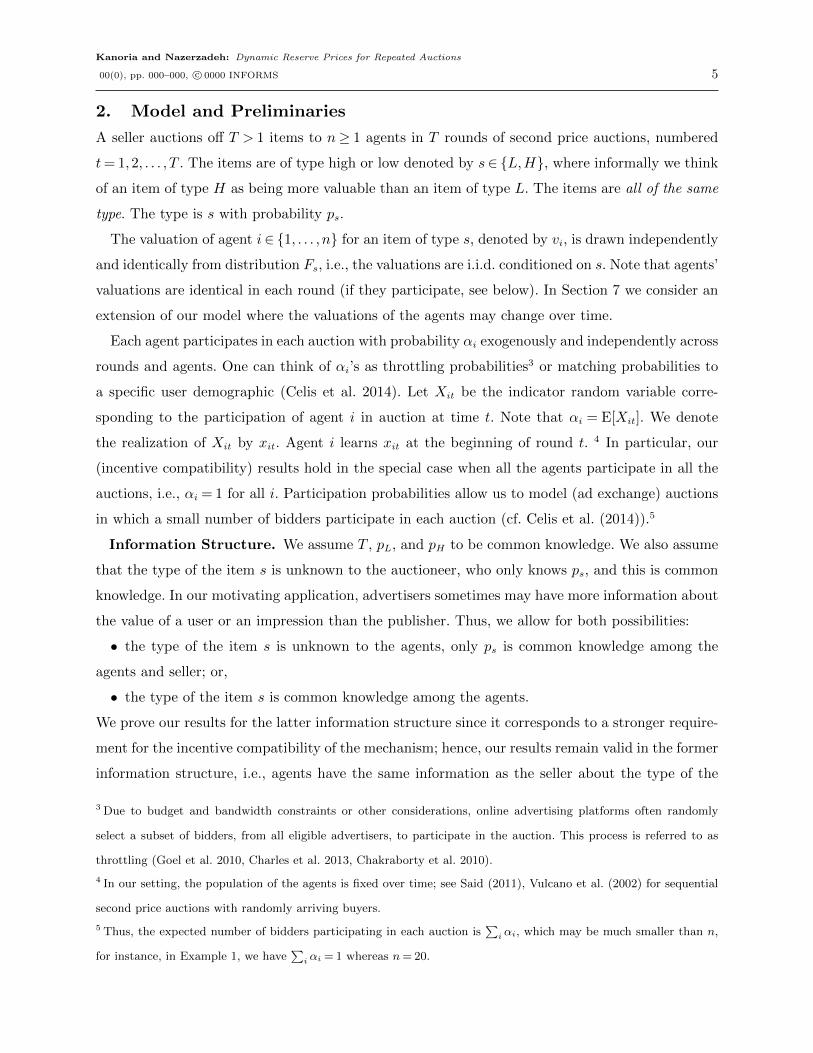
Example 1 Suppose FL is the normal distribution, with mean 1 and standard deviation 0.4,

truncated to interval [0,3], and FH =N (3,0.82), i.e., normal with mean 3 and standard deviation

0.8, and that pL = pH = 0.5. These distributions are shown in Figure 4. Also, let nα = 1, αi = α

for all i. This means that, on average, one agent participates in each round. Note that each agent

participates in αT = T/n rounds on average, making it non-trivial to have dynamic reserves without

losing incentive compatibility if T/n is much larger than 1.

We have r?L ≈ 0.796 and r?H ≈ 2.318. Using a threshold of ρ= 3 gives n0 ≈ 19.52. Using n= 20,

we obtain T0 ≈ 6800 for ε = 0.009 so we consider T = T0 = 6800. Theorem 3 guarantees that

M(ρ, r?L, r?H) is ε-incentive compatible and that the loss relative to the upper-bound benchmark

revenue is ε= .009 at most per round. Using numerical computations, we find that the (optimal)


12 00(0), pp. 000–000, c© 0000 INFORMS

Figure 1 Illustration of distributions in Example 1. FL is the normal distribution, with mean 1 and standard

deviation 0.4, truncated to interval [0,3], and FH = N (3,0.82), i.e., normal with mean 3 and standard

deviation 0.8. We use ρ= 3.

static second price auction obtains average-revenue per-round revenue equal to 0.755 using (con-

stant) reserve price 1.05. MechanismM(ρ, r?L, r?H) is found to yield a per-round revenue of 0.935 in

simulations, improving more than 23% over the static mechanism. The per-round revenue of the

optimal mechanism that knows the type of the impressions is equal to 0.938 (the 95% confidence

error in estimating the revenues is less than 0.007).

The average surplus of a buyer per round of participation, averaged over s and vi is found to be

0.335 (with 95% confidence error 0.002). Given this, and the fact that the mechanism is (provably)

(ε= 0.009)-incentive compatible, truthful bidding appears quite plausible.

5. Dynamic Incentive Compatibility

In this section, we show that, with high probability, no agent has a large incentive to deviate from

the truthful strategy in later rounds after acquiring new information. We also relax the requirement

that FL needs to have bounded support.

We start by defining a stronger notion of incentive compatibility. By a realization, denoted

by (vi, xTi )ni=1, we refer to a valuation vector (v1, v2, . . . , vn) along with a participation vector

(xT1 , xT2 , . . . , x

Tn ).

Definition 3 (Dynamic Incentive Compatibility) We call a realization ε-dynamic-incentive-

compatible (ε-DIC) with respect to a mechanism, if truthfulness, for each agent i and in each round

t∈ 1,2, . . . , T, remains an (additive) εαi(T − t)-best-response to the truthful strategy of the other

agents. We say that a mechanism is (δ, ε)-dynamic-incentive-compatible if the probability of the

realization being ε-DIC with respect to the mechanism is at least 1− δ.

Thus, in a (δ, ε)-dynamic-incentive-compatible mechanism, assuming truthful bidding, with prob-

ability at least 1− δ, the realization satisfies the following property: for each agent and each round


00(0), pp. 000–000, c© 0000 INFORMS 13

that the agent participates, the average cost of truthful bidding is at most ε for each future round

that he may participate in, relative to any other strategy. The above definition extends the notion

of (exact) interim dynamic incentive compatibility (Bergemann and Valimaki 2010) which implies

that the agents will not deviate from the truthful strategy even as they obtain more information

over time.

Theorem 4 Fix ρ ∈ (0,∞). Let λ= 1−FL(ρ). Consider any ε < r?H − r?L and let δ = ε/(r?H − r?L)

and α= miniαi > 0. Then, Mechanism M(ρ, r?L, r?H) is (δ, ε)-dynamic incentive compatible for all

n∈ [n1, n2] and T ≥ T1 where

n1 ≡ 1 +3.18 log(2/δ)

(1−FH(ρ))<∞ ,

n2 ≡δ(r?H − r?L)

λr?H,

T1 ≡4

δ

⌈n1− 1

(n− 1)α

⌉.

Further, under truthful bidding, the expected revenue of the mechanism is additively within εT of

the upper-bound benchmark revenue.

Note that this theorem requires n to be not too large, to ensure that a valuation exceeding ρ

is unlikely under s= L. The assumed upper bound on n can be eliminated in two different ways:

In the corollary below, we assume a bounded support for FL leading to λ= 0⇒ n2 =∞. Later in

Section 6, we introduce a generalized threshold mechanism, which then facilitates a result similar

to Theorem 4 while allowing n to be arbitrarily large (Theorem 5).

Corollary 2 (Bounded Support) Let FL be supported on [0, L], for L <∞. Fix ρ ∈ [L,∞).

Consider any ε < r?H − r?L and let δ= ε/(r?H − r?L). Then, Mechanism M(ρ, r?L, r?H) is (δ, ε)-dynamic

incentive compatible for all n≥ n1 and T ≥ T1 where

n1 ≡ 1 +3.18 log(2/δ)

(1−FH(ρ))<∞ ,

T1 ≡4

δ

⌈n1− 1

(n− 1)α

⌉.

Further, the expected revenue of the mechanism is additively within εT of the upper-bound bench-

mark revenue under truthful bidding.

Comparing with Theorem 3, we see that the cost of the stronger notion of equilibrium in the

above results is only a factor 2 loss in n1 and a further factor 2 loss in T1.

We prove Theorem 4 in the appendix. (Corollary 2 is immediate from Theorem 4.) We state

below the main lemma and key ideas leading to a proof of dynamic incentive compatibility for

s=H.


14 00(0), pp. 000–000, c© 0000 INFORMS

Let Qt be the event that the reserve in round t+ 1 is r?H assuming truthful bidding (thus Qt,

here, is the event that a agent with valuation exceeding ρ participates in one of the first t rounds).

Let Q∼it be the event that the reserve in round t+1 would have been r?H assuming truthful bidding

even if the bids of agent i are removed (thus Q∼it , here, is the event that a agent j 6= i with valuation

exceeding ρ participates in one of the first t rounds). Let

tδ = mint : ∃i s.t. Pr(Q∼it

∣∣s=H)≥ 1− δ (2)

(It turns out that tδ ≤ d n1−1(n−1)α

e). By definition, Qt ⊇Q∼it for all i and all t. It follows that Pr(Qtδ |s=

H)≥ 1− δ, so, in establishing (δ, ε)-dynamic incentive compatibility, we can ignore the trajectories

under which Qtδ does not occur (these trajectories have combined probability bounded above by

δ). Under Qtδ , the reserve in round tδ + 1 (and all later rounds) is already r?H , making truthful

bidding an exact best response in those rounds. Also, for agents whose valuation is less than ρ,

truthful bidding is always a best response. Consider an agent i with valuation exceeding ρ. Once i

has bid truthfully the first time, future bids of i have no impact on the reserve (which is already

r?H) and truthful bidding is a best response.11 Hence, we only need to consider the first time that i

participates (and if the reserve is still r?L). Thus, it suffices to show that under s=H for t≤ tδ, if an

agent i participates for the first time in round t, truthful bidding is an (α(T − tδ)ε)-best-response

to the truthful strategy of the other agents (even if the reserve is still r?L in round t). The following

lemma establishes that this is the case (the idea is that the reserve is very likely to rise to r?H by

the end of round τ , irrespective of the bidding behavior of agent i).

Lemma 1 Assume that s=H, n≥ n1 , δ < 1. Let tδ be defined as in Eq. (2). For any agent with

valuation exceeding ρ who participates for the first time in a round t≤ tδ, and sees a reserve r?L,

truthful bidding is (additively) α(T − tδ)δ(r?H − r?L)-optimal, assuming that others bid truthfully.

Further, we have tδ ≤ τ =⌈

(n1−1)

(n−1)α

⌉and Pr(Qtδ |s=H)≥ 1− δ.

Lemma 1 is proved in Appendix A.5.

6. The Generalized Threshold Mechanism

We now present a generalization of the threshold mechanism that allows us to eliminate the upper

bound on n in Theorem 4. (Alternatively, one can interpret Theorem 5 below as allowing FL to

have a larger tail.)

11 In the present setting with mechanism M(ρ, r?L, r?H), agent i will see a reserve that has already risen to r?H in each

subsequent round that i participates in. (Later we will generalize the threshold mechanism in Section 6, but it will

still be true that if i bids above ρ once, future bids of i will not affect the reserve, hence truthful bidding will be

exactly optimal in subsequent rounds.)


00(0), pp. 000–000, c© 0000 INFORMS 15

The generalized threshold mechanism is defined by four parameters and is denoted by

M(ρ, rL, rH , k) where rL is the initial reserve price. The reserve stays rL until k distinct agents bid

above ρ (possibly in different rounds). If this occurs then for all subsequent rounds, the reserve

price will increase to rH .

Theorem 5 Let λ = 1 − FL(ρ). Assume λ ≤ (1 − FH(ρ))/18. Fix positive ε < r?H − r?L. Define

δ= εmin(1/(r?H − r?L),2/r?H) and α= miniαi > 0. Let

n3 ≡ 1 + 8.48 log(2/δ)/(1−FH(ρ))<∞ ,

n4 ≡ 0.56 log(2/δ)/λ ,

n≡max(n3, n4) ,

T1 ≡4

δ

⌈n3− 1

(min(n, n)− 1)α

⌉.

We provide mechanisms that work well for any n≥ n3 and T ≥ T1.

• Suppose n3 <n4. For all n∈ [n3, n4] and T ≥ T1 = 4δ

⌈n3−1

(n−1)α

⌉, the generalized threshold mecha-

nism M(ρ, r?L, r?H ,2.26 log(2/δ)) is (δ, ε)-dynamic incentive compatible, and it is additively εT close

to the revenue benchmark under truthful bidding.

• For all n ≥ max(n3, n4) and T ≥ T1 = 4δ

⌈n3−1

(n−1)α

⌉, the generalized threshold mechanism

M(ρ, r?L, r?H ,4λn) is (δ, ε)-dynamic incentive compatible, and it is additively εT close to the upper-

bound revenue benchmark under truthful bidding.

As a remark to ease the burden of notation: note that T1 ≤ 4δ

⌈1α

⌉for the n values of interest, i.e.,

for n≥ n3. In other words, 4δ

⌈1α

⌉rounds suffice to obtain our positive results. Also, note that for

nα= Θ(1), we still have n3 =O(log(1/δ)) and T1 =O(log(1/δ)/δ) as was the case for Theorem 3,

so our requirements on the number of agents and number of rounds continue to be reasonable.

7. Discussion

Transient Valuations So far we assumed that the valuations of the agents are constant over

time. In this section, we consider the following extension of our model: each time an agent j

participates, he draws a new valuation from Fs independently with some probability βj (our original

model corresponds to the case βj = 0), and retains his previous valuation with probability 1− βj.As we show in Appendix A.6, our incentive compatibility results of Theorem 3 and Corollary 2

(for a bounded low type distribution) still hold in this setting. It turns out that the incentive of

the agents to deviate is even smaller and the proofs work nearly as before for any βj’s in [0,1].

On the other hand, the following example shows that with transient valuations, a mechanism

that is not ex-post individually rational can obtain a revenue higher than the “upper bound”


16 00(0), pp. 000–000, c© 0000 INFORMS

benchmark, (cf. Section 3) by charging the agents a high price in advance: Suppose there is only

one agent (n= 1), the agent participates in all rounds (α= 1), and the agent draws a new valuation

in each round from the uniform distribution over [0,1] (i.e., β = 1). It is not difficult to see that

the optimal constant reserve for this setting is equal to 12

which yields an expected revenue of T4

since the agent will purchase the item with probability 12. Now consider a mechanism that offers

reserve price T−12− ε (for an arbitrarily small ε) in the first round; if the agent accepts that price,

the mechanism offers the item for free in the future rounds, whereas if the agent refuses the offer,

the mechanism posts a price of 1 in each future round. Observe that the agent will accept the

mechanism’s offer in the first round and the revenue obtained in this case is equal to T−12−ε, which

exceeds T/4 for large enough T and small ε. However, this mechanism is not ex-post individually

rational in each round. For β ∈ (0,1) the optimal mechanism (that does not satisfy the ex-post IR

property) would take the form of contracts followed by a sequence of auctions (Battaglini 2005,

Kakade et al. 2013, Pavan et al. 2014).

Robustness of the threshold mechanism The generalized threshold mechanism only con-

siders the maximum bid submitted by each bidder thus far, and combines the highest among these

maximum bids suitably to determine the reserve price for the current round. This mechanism is

robust in the following ways:

• The mechanism is unaffected by the creation of fake bidders who may only bid low values with

the intention of misleading the seller into believing that the type of the item is L, without winning

the auction. A mechanism which relies, for instance, on the average/typical behavior of a bidder

would be vulnerable to this. (Note that bidders never want to mislead the seller into thinking that

the item type is H, so they would not want to create fake bidders who bid high values.)

• Bidders cannot benefit from the use of multiple identities: this can only increase the likelihood

that the reserve price rises.

We expect that the principle underlying our mechanism has further robustness properties:

• If the type of the item is subject to change (slowly) over time this can be handled by only

using “recent” bids to determine the reserve price, where recency is determined by using a window

of appropriate length. We expect that our results will generalize to such an environment.

• We expect that even with a continuum of types, a mechanism that is similar in spirit will

do well. Such a mechanism may determine the reserve as a suitable continuous function of the

k highest bids submitted by distinct bidders, for appropriately chosen k. We expect that good

incentive and revenue properties will again emerge for relatively small values of n and T , though

rigorous analysis appears complicated.


00(0), pp. 000–000, c© 0000 INFORMS 17

The size of n and T needed We believe that the size of n and T required for our results

(from conservative theoretical bounds) are practical (∼ 10 and ∼ 10000 respectively), cf. Example

1. Most advertisers participate in hundreds of thousands and sometimes millions of auctions. The

pool of advertisers that are interested in certain impression types is often large. We also point out

that even for large values of n, for small α (e.g., αn= 1), the number of advertisers that participate

in each auction is small (mirroring reality), therefore, the reserve prices will have significant impact

on revenue.

Connection to Mean Field Equilibrium We now comment briefly on the connection between

our work and the concept of mean field equilibrium. A number of recent papers study notions of

mean field equilibrium, e.g., Iyer et al. (2011), Balseiro et al. (2013) study mean field equilibria

in dynamic auctions, and Gummadi et al. (2013) studies mean field equilibrium in multiarmed

bandit games. An agent making a mean field assumption assumes that the set of competitors (or

cooperators) she faces will be drawn uniformly at random from a large pool of agents with a known

distribution of types. In our work, agents’ participate in a particular round of a dynamic auction

independently at random, but our results do not require n→∞ and agents retain their valuation

for all rounds in which they participate. In Theorem 4, one can have any fixed number of agents

exceeding n1 =O(log(1/ε)), and participants reason about the posterior distribution of competitors

they will face in a round, given the information available to them. This posterior distribution of

the valuations of competitors is in general different from the prior distribution of valuations and

evolves from one round to the next, in contrast with mean field analyses.

8. Conclusion

We considered repeated auctions of items, all of the same type, with the auctioneer not knowing

the type of the items a-priori. In our model, the issue of incentives is challenging because a bidder

typically participates in multiple auctions, and is hence sensitive to changes in future reserve prices

based on current bidding behavior. We demonstrated a fairly broad setting in which a simple

dynamic reserve second price auction mechanism can lead to substantial improvements in revenue

over the best fixed reserve second price auction. In fact, our threshold mechanism is approximately

truthful and achieves near optimal revenue in our setting. We demonstrate a numerical illustration

of our results with a reasonable choice of model parameters, and show significant improvement in

revenue over the static baseline.

In future work, we would like to investigate the effects of various properties of the (joint) dis-

tributions of the valuation of the advertisers (e.g., more than two types), the characteristics of

learning algorithms (beyond simple threshold mechanisms), and the effect of the rate (and manner)


18 00(0), pp. 000–000, c© 0000 INFORMS

in which the valuations of advertisers change over time on the equilibrium and the revenue of the

auctioneer.

Acknowledgment We would like to thank Brendan Lucier, Mohammad Mahdian, Mukund

Sundararajan, and Ramandeep Randhawa for their insightful comments and suggestions. This work

was supported in part by Microsoft Research, New England. The work of the second author was

supported by a Google Faculty Research Award.

Appendix

A. Proofs

A.1. Proof of Proposition 1

The following is the key lemma leading to Proposition 1.

Lemma 2 (Upper-bound) LetMsT be the optimal T -round mechanism that knows the type of the item, s.

Similarly,Ms1 corresponds to the optimal (static) mechanism when T = 1. Then, the revenue ofMs

T , denoted

by Rev(MsT ), is bounded by T ×Rev(Ms

1). Furthermore, if mechanism Ms1 is ex-post incentive compatible,

then, MsT can be implemented by repeating mechanism Ms

1 at each step t= 1, · · · , T .

Proof of Lemma 2. To prove the first part of the claim, we construct mechanism M that obtains, in

expectation, revenue equal to Rev(MsT )/T . Since by definition Rev(Ms

1) is the optimal revenue that can

be obtained when T = 1, we conclude that Rev(MsT )≤ T ×Rev(Ms

1).

We construct mechanism M as follows: Let B ⊆ 1, · · · , n be the set of agents who participate in the

one-round auction. Note that each agent i knows his own xit but not xjt for any other agent j 6= i. For all

agents j /∈B, draw a (hypothetical) valuation i.i.d. from the distribution of valuations Fs. Now consider the

probability space generated by simulating mechanismMsT over a T round auction by sampling Xjt’s in each

round and emulating the (optimal) bidding strategy of the agents under MsT .

Consider the distribution DB of (qB, pB) in rounds where the set of agents who participate is exactly B, in

this probability space. More precisely, we are considering not a single simulation, but the probability space

of possible simulation trajectories. For each trajectory ω, the pair (qB, pB) for each round in which agents B

participate contributes a weight in H proportional to the probability of trajectory ω.

To determine the payments under M, draw (qB, pB) uniformly from distribution DB. The mechanism M

charges the agents in B these amounts pB and allocate the items according to qB.

We argue that the mechanism M is truthful: It is not hard to see that the ex interim expected utility of an

agent i from participating in M with bid bi when others bid truthfully, is exactly 1/T times the ex interim

expected utility of participating inMsT and following his equilibrium strategy for valuation bi there if others

follow their equilibrium strategies. Recall that each agent i knows his own xit but not xjt for any other agent

j 6= i. It follows that truthful bidding is an equilibrium in mechanism M. Further, under truthful bidding, it


00(0), pp. 000–000, c© 0000 INFORMS 19

is not hard to see that the expected revenue of mechanism M is Rev(MsT )/T , as claimed. Note that when

αi = 1, 1≤ i≤ n, the proof would be simplified and could be argued using the revelation principle Myerson

(1986).

We now prove the second part of the claim. Note that ifMs1 is ex-post incentive compatible, the leakage of

information from one round to another does not change the strategy of the agents. For private value settings

such as this, ex-post incentive compatibility implies that truthfulness is a (weakly) dominant strategy for

each agent for any realizations of other agents’ valuations. Therefore, repeating mechanism Ms1 obtains

revenue T ×Ms1 which is the upper-bound revenue.

Proof of Proposition 1. When Fs is regular and s is known, we know that the optimal mechanism for a

single round is a second price auction with reserve r?s . Now, this mechanism is ex-post incentive compatible.

The result then follows immediately from Lemma 2.

A.2. Proof of Theorem 3

In Appendix A.5, we prove the following lemma.

Lemma 3 Fix any C <∞. Assume s = H, n ≥ n0 ≡ 1 + C log(2/δ)/(1 − FH(ρ)). Fix an agent i. With

probability at least 1− (δ/2)C/1.59 at least one agent j 6= i with valuation exceeding ρ will bid in the first

τ =⌈

n0−1(n−1)α

⌉rounds. For k ≤ C log(2/δ)/3.18, at least k agents different from i with valuation exceeding ρ

will bid in the first τ =⌈

n0−1(n−1)α

⌉rounds with probability at least 1− (δ/2)C/4.24.

Here we have used 1/(1− e−1)< 1.59. We now show how the lemma, for k= 1, implies the results.

Proof of Theorem 3. We now prove Theorem 3 by first showing that the threshold mechanism is ε-

incentive-compatible. First assume s = L. Consider any agent i with valuation vi ∈ [0, L] and assume that

other agents are truthful always. Since vi ≤ ρ, it is clear that truthful bidding weakly dominates any other

strategy, since this is true myopically, the reserve is unaffected, and the bidding behavior of others is unaf-

fected by the bids of agent i. In this case, the reserve remains r?L and the agents bid truthfully throughout,

so there is no loss in revenue.

Now assume s=H. Agent i being truthful can cause the reserve to rise though it wouldn’t otherwise have

risen, leading to a loss of at most (r?H − r?L)αiτ ≤ αiεT

2in expected utility for the agent during the first τ

rounds. If the reserve would not have risen in the first τ rounds but agent i caused it to rise, this can lead

to a further loss of up to (r?H − r?L) per round of participation, and such a loss occurs with probability at

most ε/(2(r?H − r?L)) from Lemma 3 (with C = 1.59), leading to a bound of αiεT

2for this loss to the agent.

Combining yields the overall bound of αiεT on the loss incurred by agent i by being truthful relative to any

other strategy for s=H.

Finally we bound the loss in revenue from using this mechanism if s=H. Recall that the optimal auction

if the auctioneer knows s=H beforehand is to commit and run a second price auction with reserve r?H in all

rounds. Hence, similar to the above, the expected revenue loss to the auctioneer is bounded by τ(r?H − r?L) +


20 00(0), pp. 000–000, c© 0000 INFORMS

ε2(r?

H−r?L

)·T (r?H − r?L)≤ εT if s=H. Since for each possible s, the expected loss in revenue is bounded above

by εT , the same bound holds when we take expectation over s.

Proof of Corollary 1. Again, the case s = L is trivial so we focus on s = H. Consider τ ′ = C logT ,

where we will choose C ∈ (0,∞) appropriately. Then, with probability at least 1− 1/T , each of the n agents

participates in at least one of the first τ ′ rounds (for large enough C). As such, with probability at least

1− 1/T , the reserve rises to r?H by the end of round τ ′ if and only if at least one agent has a valuation

exceeding ρ. Now, if no agent has valuation exceeding ρ, the benchmark mechanism extracts no revenue

(under the assumption ρ≤ r?H) so there is no loss in revenue from not increasing the reserve. We conclude

that, with probability at least 1− 1/T , there is no loss in revenue relative to the benchmark after round τ ′.

We conclude that the ratio of the expected mechanism revenue (under truthful bidding) to the benchmark

revenue is at least 1−O(τ ′/T + 1/T ) = 1−O(logT/T ).


First assume s=L. A simple union bound ensures that all agents have a valuation not greater than ρ with

probability at least 1−λn≥ 1− δ(r?H − r?L)/r?H , in which case truthful bidding weakly dominates any other

strategy. (Since vi ≤ ρ, it is clear that truthful bidding weakly dominates any other strategy, since this is true

myopically and the bidding behavior of others is unaffected by the bids of agent i.) Hence, the realization

is 0-DIC with respect to the mechanism with probability at least 1− δ(r?H − r?L)/r?H ≥ 1− δ. Further, we

can easily bound the loss in expected revenue relative to the benchmark under truthful bidding: There is

no loss with probability 1− δ(r?H − r?L)/r?H (the mechanism matches the benchmark mechanism, since the

reserve remains r?L throughout) and a loss of at most r?HT (due to the reserve rising to r?H) with probability

δ(r?H − r?L)/r?H . Thus, the loss in expected revenue is bounded by δ(r?H − r?L)T = εT as required.

Now assume s=H. For any agent with a valuation less than or equal to ρ, truthful bidding again weakly

dominates any other strategy, since this is true myopically and the bidding behavior of others is unaffected

by the bids of agent i. It remains to deal with agents whose valuation exceeds ρ, to establish that truthful

bidding is (δ, ε)-incentive-compatible. In particular, we need to show that with probability at least 1− δ, the

realization is ε-DIC with respect to the mechanism, i.e., that each such agent i loses no more than αi(T − t)ε

in expectation on the equilibrium path from bidding truthfully in round t, for each t that i participates in.

But this follows from Lemma 1: all realizations such that Qtδ occurs are ε-DIC, and Pr(Q(tδ))≥ 1− δ. See

the argument after the statement of Theorem 4 in Section 4 for further details.

It remains to show that the loss in revenue is no more than εT , assuming truthful bidding under ε-DIC

realizations. Now, using Lemma 3 with C = 3.18 and Qt ⊇Q∼it , we have

Pr(Qτ )≥ 1− (δ/2)2 ≥ 1− δ/2 .

Under Qτ , the mechanism matches the benchmark mechanism for rounds after τ and hence there is no loss

in revenue relative to the benchmark, after the first τ rounds. In any round, the loss due to setting the


00(0), pp. 000–000, c© 0000 INFORMS 21

wrong reserve (under truthful bidding) is bounded by r?H − r?L. Under Qτ (the complement of Qτ ), the loss

can be this large in each of T rounds, in worst case. It follows that the overall loss in revenue is bounded

by (r?H − r?L)(τ + Pr(Qτ )T ). But by definition, τ = δT1/4≤ Tδ/4 and Pr(Qτ )≤ δ/2, implying that the loss

in revenue relative to the benchmark is at most (r?H − r?L)δ(3/4)T = (3/4)εT ≤ εT as required, using the

definition of δ.


We start with the first bullet. The proof for s=H follows exactly the same steps as the proof of Theorem 4,

except that we use of the second part of Lemma 3 (using n≥ n3) with k= 2.26 log(2/δ)≤ (C/3.18) log(2/δ)

for C = 8.48, instead of the first part of the lemma (corresponding to k= 1). Consider s=L. The probability

of k or more agents with valuation exceeding ρ is Pr(Binomial(n,λ)≥ k). Since n≤ n4, we have the mean

of the binomial µ= nλ≤ µ0 = 0.56 log(2/δ), in particular, k ≥ 4µ0 ≥ 4µ. Now, using a Chernoff bound (on

Binomial(n,λ0) where λ0 = µ0/n≥ λ leading to a mean of µ0; clearly this binomial stochastically dominates

the one we care about), we infer that

Pr(Binomial(n,λ)≥ k) ≤Pr(Binomial(n,λ0)≥ k)

≤ exp−µ0 · 32/(2 + 3)= exp−0.56 log(2/δ) · 9/5

≤ exp−1.00 log(2/δ)= δ/2 .

If all valuations are no more than ρ then such a realization is clearly 0-DIC (i.e., incentive compatible in an

exact sense) with respective to the mechanism. Hence, we have shown that the probability of the realization

being ε-DIC is at least 1− δ/2, implying (δ, ε)-dynamic incentive compatibility for s= L. Further, the loss

in revenue for s=L under truthful bidding is bounded above by r?H per round for cases in which k or more

agents have valuation exceeding ρ, and there is no loss otherwise. Hence, the overall loss in expected revenue

is bounded above by (δ/2)Tr?H ≤ εT (using δ≤ 2ε/r?H) as required.

Now consider the second bullet. Consider s = H. The threshold is k = 4λn. Let n = maxn3, n4. The

following lemma is similar to Lemma 3, but allows for larger values of k. The proof is in Appendix A.5.

Lemma 4 Assume s = H, n ≥ n ≥ n0 ≡ 1 + C log(2/δ)/(1− FH(ρ)) and k ≤ C log(2/δ)n/(3.18n). Fix an

agent i. With probability at least 1− (δ/2)C/4.24, at least k agents different from i with valuation exceeding ρ

will bid in the first τ =⌈

n0−1(n−1)α

⌉rounds.

To use Lemma 4 we need an upper bound on n. Note that using δ≤ 1 and FH(ρ)≥ 0, we have log(2/δ)/(1−

FH(ρ))≥ log 2. Hence we have

n3 ≤log(2/δ)

1−FH(ρ)(8.48 + 1/ log 2)≤ 10.0 log(2/δ)

1−FH(ρ)≤ log(2/δ)

1.8λ

using λ≤ (1−FH(ρ))/18. It follows that n≤ log(2/δ)

1.8λ. With reference to the upper bound on k in Lemma 4,

we deduce that

8.48 log(2/δ)n/(3.18n)≥ 2.26 log(2/δ)n/n≥ 2.26 · 1.8λn≥ 4λn.


22 00(0), pp. 000–000, c© 0000 INFORMS

Hence, using Lemma 4, we deduce that under truthful bidding, the reserve rises to rH by the end of τ =

4δ

⌈n3−1

(n−1)α

⌉rounds with probability at least 1− (δ/2)2. Following the argument in the proof of Lemma 1 from

here and using δ ≤ ε/(r?H − r?L), we deduce (δ, ε)-dynamic incentive compatibility for s=H. We also deduce

that the loss in expected revenue is small, similar to the proof of Theorem 4.

Consider the second bullet and s=L. The probability of k= 4λn or more agents with valuation exceeding

ρ is Pr(Binomial(n,λ)≥ 4λn). The mean µ= λn≥ 0.56 log(2/δ) since n≥ n≥ n3. We infer using a Chernoff

bound that

Pr(Binomial(n,λ)≥ 4λn) ≤ exp−µ · 32/(2 + 3) ≤ exp−0.56 log(2/δ) · 9/5

≤ exp−1.00 log(2/δ)= δ/2 .

We then complete the proof of approximate dynamic incentive compatibility and revenue optimality exactly

as we did for the first bullet with s=L.

A.5. Proofs of Lemmas

Proof of Lemma 1. Consider any agent i. By definition of tδ, we know that for t≤ tδ, for all agents i we

have

Pr(Q∼it−1)> δ , (3)

where Q∼it−1 is the complement of Q∼it−1.

Let τ = d n1−1(n−1)α

e. Note that τ ≤ δT1/4≤ δT/4⇒ τ ≤ δ(T − τ)/2. It follows from Lemma 3 that

Pr(Q∼iτ )≤ δ2/2 (4)

In particular, we have tδ < τ and Pr(Qτ )≥Pr(Q∼iτ )≥ 1−δ2/2≥ 1−δ, yielding the second part of the lemma.

Combining Eqs. (3) and (4) we obtain that

Pr(Q∼iτ |Q∼it−1)≤Pr(Q∼iτ )/Pr(Q∼it−1)≤ (δ2/2)/δ = δ/2 . (5)

Hence, agent i who participates for the first time in round t and sees reserve r?L, infers that the reserve will

rise to r?H by round τ + 1 with probability at least 1− δ/2, due to the bids of other agents. Thus, we can

bound the expected cost in future rounds to agent i by causing the reserve to rise by bidding truthfully:

• Under Q∼iτ , agent i may lose at most αi(T − t)(r?H − r?L) in future rounds (in expectation).

• Under Q∼iτ , agent i may lose at most αi(τ − t)(r?H − r?L)≤ αiτ(r?H − r?L) in rounds only up to round τ .

Thus, the overall future cost of bidding truthfully is bounded by

Pr(Q∼iτ )αiτ(r?H − r?L) + Pr(Q∼iτ )αi(T − t)(r?H − r?L)≤ 1 ·αi(r?H − r?L)δ(T − τ)/2 + (δ/2) ·αi(T − t)(r?H − r?L)

≤ δαi(T − t)(r?H − r?L)

as required. Here we used τ ≤ δ(T − τ)/2 and t≤ τ from the discussion above.

Proof of Lemma 3. Let Q∼iτ (k) denote the event of interest, and Q∼iτ be the event for k = 1. For each

agent j 6= i, agent j participates in some round t′ for t′ ≤ τ with probability 1− (1− αj)τ ≥ 1− (1− α)τ .


00(0), pp. 000–000, c© 0000 INFORMS 23

Independently, agent j has a valuation exceeding ρ with probability 1−FH(ρ). Hence, we have vj ≥ ρ and

agent j enters a bids before the end of round τ , with probability at least (1− (1− α)τ )(1− FH(ρ)), and

this occurs independently for j 6= i. Note that (1− x)1/x ≤ e−1 for x ∈ (0,1) since (1− x)1/x is monotone

decreasing in x. Using this bound, we have

1− (1−α)τ ≥ 1− exp(−ατ)

≥ 1− exp(−(n0− 1)/(n− 1))

≥ n0− 1

n− 1(1− exp(−1))

≥ n0− 1

1.59(n− 1), (6)

where we also used the definition of τ and convexity of f(x) = exp(−2kx).

It follows that

Pr(Q∼iτ )≤Pr(

Binomial(n− 1, [1− (1−α)τ ][1−FH(ρ)]

)= 0

)=(

1− [1− (1−α)τ ][1−FH(ρ)])n−1

. (7)

Hence,

Pr(Q∼iτ )≤ exp

[1− (1−α)τ ][1−FH(ρ)](n− 1)

≤ exp− (n0− 1)(1−FH(ρ))/1.59

≤ exp−(C/1.59) log(2/δ)= (δ/2)C/1.59 ,

using n0 ≥ 1 +C log(2/δ)/(1−FH(ρ)) and Eq. (6).

Similarly,

Pr(Q∼iτ (k))≤Pr(

Binomial(n− 1, [1− (1−α)τ ][1−FH(ρ)]

)< k

)=(

1− [1− (1−α)τ ][1−FH(ρ)])n−1

. (8)

The mean of the binomial is

µ= (n− 1)[1− (1−α)τ ][1−FH(ρ)]≥ (n0− 1)[1−FH(ρ)]/1.59 =C log(2/δ)/1.59

using Eq. (6). It follows using a Chernoff bound and k≤C log(2/δ)/3.18≤ µ/2 that

Pr(Q∼iτ (k))≤ exp−µ(1− 1/2)2/2= exp−C log(2/δ)/4.24= (δ/2)C/4.24.

Proof of Lemma 4. The proof is very similar to the proof of Lemma 3. Let Q∼iτ (k) denote the event of

interest. For each agent j 6= i, agent j participates in some round t′ for t′ ≤ τ with probability 1− (1−αj)τ ≥1− (1−α)τ . Proceeding as before, we have

1− (1−α)τ ≥ n0− 1

1.59(n− 1). (9)


24 00(0), pp. 000–000, c© 0000 INFORMS

We have Eq. (8) for the probability of Q∼iτ (k) as before. The mean of the binomial is

µ= (n− 1)[1− (1−α)τ ][1−FH(ρ)]≥ (n0− 1)[1−FH(ρ)](n− 1)/(1.59(n− 1))

=C log(2/δ)(n− 1)/(1.59(n− 1))≥C log(2/δ)n/(1.59n) (10)

using Eq. (9) and n≥ n.

It follows using a Chernoff bound and k≤C log(2/δ)n/(3.18n)≤ µ/2 that

Pr(Q∼iτ (k))≤ exp−µ(1− 1/2)2/2= exp−C log(2/δ)/4.24= (δ/2)C/4.24 , (11)

using n≥ n.

A.6. Transient valuations

Consider the case where, each time an agent i participates, with probability βi ∈ [0,1], he draws a new

valuation from distribution Fs. We show that Theorem 3 and Corollary 2 hold also in this case (i.e., our

results with bounded low type distribution continue to hold). The following lemma (similar to Lemma 3 and

proved using it) is a key building block.

Lemma 5 Fix any C <∞. Assume s=H, n≥ n0 ≡ 1 +C log(2/δ)/(1−FH(ρ)). Consider transient valua-

tions with resampling probability βj for agent j. Fix an agent i. With probability at least 1− (δ/2)C/1.59 at

least one agent j 6= i with valuation exceeding ρ (in that round) will bid in the first τ =⌈

n0−1(n−1)α

⌉rounds.

Proof of Lemma 5. Compare with the case of fixed valuations in Lemma 3. Couple the two systems such

that the valuation of agent j when j participates for the first time with transient valuations, is the same as

the valuation of j with fixed valuations. Then if the event “at least one agent j 6= i with valuation exceeding

ρ (in that round) will bid in the first τ rounds” occurs with fixed valuations, it also occurs with transient

valuations. The result follows from the first part of Lemma 3.

Now, using this lemma, the proof of Theorem 3 goes through verbatim. The proof of Theorem 4 for s=H

also goes through verbatim, whereas the case s= L is trivial under a bounded low type distribution as in

Corollary 2, implying that Corollary 2 also holds with transient valuations.

References

Alessandro Acquisti and Hal R. Varian. Conditioning prices on purchase history. Marketing Science, 24(3):

367–381, May 2005.

Kareem Amin, Afshin Rostamizadeh, and Umar Syed. Learning prices for repeated auctions with strategic

buyers. In Christopher J. C. Burges, Leon Bottou, Zoubin Ghahramani, and Kilian Q. Weinberger,

editors, NIPS, pages 1169–1177, 2013.


00(0), pp. 000–000, c© 0000 INFORMS 25

Aaron Archer, Christos Papadimitriou, Kunal Talwar, and Eva Tardos. An approximate truthful mechanism

for combinatorial auctions with single parameter agents. Internet Mathematics, 1(2):129–150, 2004.

Yossi Aviv and Amit Pazgal. Optimal Pricing of Seasonal Products in the Presence of Forward-looking

Consumers. 10(3):339–359, 2008. ISSN 1526-5498.

Yossi Aviv, Mingcheng Wei, and Fuqiang Zhang. Responsive pricing of fashion products: The effects of

demand learning and strategic consumer behavior. 2013.

Santiago Balseiro, Jon Feldman, Vahab S. Mirrokni, and S. Muthukrishnan. Yield optimization of display

advertising with ad exchange. In Shoham et al. (2011), pages 27–28. ISBN 978-1-4503-0261-6.

Santiago R. Balseiro, Omar Besbes, and Gabriel Y. Weintraub. Auctions for online display advertising

exchanges: Approximations and design. In Proceedings of the Fourteenth ACM Conference on Electronic

Commerce, EC ’13, pages 53–54, New York, NY, USA, 2013. ACM. ISBN 978-1-4503-1962-1.

David P. Baron and David Besanko. Regulation and information in a continuing relationship. Information

Economics and Policy, 1(3):267–302, 1984.

Marco Battaglini. Long-term contracting with markovian customers. American Economic Review, 95(3):

637–658, 2005.

Dirk Bergemann and Juuso Valimaki. The dynamic pivot mechanism. Econometrica, 78:771–789, 2010.

Omar Besbes and Assaf Zeevi. Dynamic pricing without knowing the demand function: risk bounds and

near-optimal algorithms. Operations Research, 57:1407–1420, 2009.

Sushil Bikhchandani and Kevin McCardle. Behavior-based price discrimination by a patient seller. B.E.

Journals of Theoretical Economics, 12, June 2012.

L. Elisa Celis, Gregory Lewis, Markus Mobius, and Hamid Nazerzadeh. Buy-it-now or take-a-chance: Price

discrimination through randomized auctions. Management Science, 2014.

Nicolo Cesa-Bianchi, Claudio Gentile, and Yishay Mansour. Regret minimization for reserve prices in second-

price auctions. In Sanjeev Khanna, editor, Proceedings of the Twenty-Fourth Annual ACM-SIAM

Symposium on Discrete Algorithms, SODA 2013, New Orleans, Louisiana, USA, January 6-8, 2013,

pages 1190–1204. SIAM, 2013. ISBN 978-1-61197-251-1. doi: 10.1137/1.9781611973105.86. URL http:

//dx.doi.org/10.1137/1.9781611973105.86.

Tanmoy Chakraborty, Eyal Even-Dar, Sudipto Guha, Yishay Mansour, and S. Muthukrishnan. Selective call

out and real time bidding. In Amin Saberi, editor, WINE, volume 6484 of Lecture Notes in Computer

Science, pages 145–157. Springer, 2010. ISBN 978-3-642-17571-8.

Denis Charles, Deeparnab Chakrabarty, Max Chickering, Nikhil R. Devanur, and Lei Wang. Budget smooth-

ing for internet ad auctions: A game theoretic approach. In Proceedings of the Fourteenth ACM Con-

ference on Electronic Commerce, EC ’13, pages 163–180, New York, NY, USA, 2013. ACM. ISBN

978-1-4503-1962-1.

http://dx.doi.org/10.1137/1.9781611973105.86

http://dx.doi.org/10.1137/1.9781611973105.86


26 00(0), pp. 000–000, c© 0000 INFORMS

Steve Chien and Alistair Sinclair. Convergence to approximate Nash equilibria in congestion games. Games

and Economic Behavior, 71(2):315327, 2011.

Vincent Conitzer, Curtis R. Taylor, and Liad Wagman. Hide and seek: Costly consumer privacy in a market

with repeat purchases. Marketing Science, 31(2):277–292, March 2012. ISSN 1526-548X.

Jose Correa, Ricardo Montoya, and Charles Thraves. Contingent preannounced pricing policies with strategic

consumers. Working Paper, 2013.

Jacques Cremer and Richard P McLean. Full extraction of the surplus in bayesian and dominant strategy

auctions. Econometrica, 56(6):1247–57, November 1988.

Constantinos Daskalakis, Aranyak Mehta, and Christos H. Papadimitriou. A note on approximate nash

equilibria. Theor. Comput. Sci., 410(17):1581–1588, 2009.

Sriram Dasu and Chunyang Tong. Dynamic pricing when consumers are strategic: Analysis of posted and

contingent pricing schemes. European Journal of Operational Research, 204(3):662–671, August 2010.

Arnoud V. den Boer. Dynamic pricing and learning: Historical origins, current research, and new directions.

Working Paper, 2014.

Nikhil R. Devanur, Yuval Peres, and Balasubramanian Sivan. Perfect bayesian equilibria in repeated sales.

CoRR, abs/1409.3062, 2014. URL http://arxiv.org/abs/1409.3062.

Rosa Branca Esteves. A survey on the economics of behaviour-based price discrimination. NIPE Working

Papers 5/2009, NIPE - Universidade do Minho, 2009.

Tomas Feder, Hamid Nazerzadeh, and Amin Saberi. Approximating nash equilibria using small-support

strategies. In Jeffrey K. MacKie-Mason, David C. Parkes, and Paul Resnick, editors, ACM Conference

on Electronic Commerce, pages 352–354. ACM, 2007. ISBN 978-1-59593-653-0.

Hu Fu, Nima Haghpanah, Jason Hartline, and Robert Kleinberg. Optimal auctions for correlated buyers with

sampling. In Proceedings of the Fifteenth ACM Conference on Economics and Computation, EC ’14,

pages 23–36, New York, NY, USA, 2014. ACM. ISBN 978-1-4503-2565-3. doi: 10.1145/2600057.2602895.

Drew Fudenberg and J. Miguel Villas-Boas. Behavior-Based Price Discrimination and Customer Recognition.

Elsevier Science, Oxford, 2007.

Ashish Goel, Mohammad Mahdian, Hamid Nazerzadeh, and Amin Saberi. Advertisement allocation for

generalized second-pricing schemes. Operations Research Letters, 38(6):571–576, 2010.

Ramki Gummadi, Peter Key, and Alexandre Proutiere. Optimal bidding strategies and equilibria in dynamic

auctions with budget constraints. Working Paper, 2013.

J. Michael Harrison, N. Bora Keskin, and Assaf Zeevi. Bayesian dynamic pricing policies: Learning and

earning under a binary prior distribution. Management Science, 58(3):570–586, 2012.

Oliver D. Hart and Jean Tirole. Contract renegotiation and coasian dynamics. Review of Economic Studies,

55:509–540, 1988.

http://arxiv.org/abs/1409.3062


00(0), pp. 000–000, c© 0000 INFORMS 27

Sebastien Hemon, Michel de Rougemont, and Miklos Santha. Approximate nash equilibria for multi-player

games. In Burkhard Monien and Ulf-Peter Schroeder, editors, SAGT, volume 4997 of Lecture Notes in

Computer Science, pages 267–278. Springer, 2008. ISBN 978-3-540-79308-3.

Krishnamurthy Iyer, Ramesh Johari, and Mukund Sundararajan. Mean field equilibria of dynamic auctions

with learning. In Shoham et al. (2011), pages 339–340. ISBN 978-1-4503-0261-6.

Sham M. Kakade, Ilan Lobel, and Hamid Nazerzadeh. Optimal dynamic mechanism design and the virtual

pivot mechanism. Operations Research, 61(4):837–854, 2013.

Michael J. Kearns and Yishay Mansour. Efficient nash computation in large population games with bounded

influence. In Adnan Darwiche and Nir Friedman, editors, UAI, pages 259–266. Morgan Kaufmann,

2002. ISBN 1-55860-897-4.

Preston McAfee. The design of advertising exchanges. Review of Industrial Organization, 39(3):169—185,

2011.

R Preston McAfee and Daniel Vincent. Updating the reserve price in common-value auctions. American

Economic Review, 82(2):512–18, May 1992.

R Preston McAfee, John McMillan, and Philip J Reny. Extracting the surplus in the common-value auction.

Econometrica, 57(6):1451–59, November 1989.

Frank McSherry and Kunal Talwar. Mechanism design via differential privacy. In Foundations of Computer

Science, 2007. FOCS’07. 48th Annual IEEE Symposium on, pages 94–103. IEEE, 2007.

Mehryar Mohri and Andres Munoz Medina. Revenue optimization in posted-price auctions with strategic

buyers. NIPS, 2014a.

Mehryar Mohri and Andres Munoz Medina. Learning theory and algorithms for revenue optimization in

second price auctions with reserve. In Proceedings of the 31th International Conference on Machine

Learning, ICML 2014, Beijing, China, 21-26 June 2014, volume 32 of JMLR Proceedings, pages 262–

270. JMLR.org, 2014b. URL http://jmlr.org/proceedings/papers/v32/mohri14.html.

S. Muthukrishnan. Ad exchanges: Research issues. In Internet and Network Economics, 5th International

Workshop (WINE), pages 1–12, 2009.

Roger Myerson. Multistage games with communications. Econometrica, 54(2):323–358, 1986.

Roger B. Myerson. Optimal auction design. Mathematics of Operations Research, 6(1):58–73, 1981.

Hamid Nazerzadeh, Amin Saberi, and Rakesh Vohra. Dynamic cost-per-action mechanisms and applications

to online advertising. Operations Research, 61(1):98–111, 2013.

Michael Ostrovsky and Michael Schwarz. Reserve prices in internet advertising auctions: A field experiment.

Working Paper, http://faculty-gsb.stanford.edu/ostrovsky/papers/rp.pdf, 2009.

Christos H. Papadimitriou and George Pierrakos. On optimal single-item auctions. In STOC, pages 119–128,

2011.

http://jmlr.org/proceedings/papers/v32/mohri14.html


28 00(0), pp. 000–000, c© 0000 INFORMS

Alessandro Pavan, Ilya Segal, and Juuso Toikka. Dynamic mechanism design: A myersonian approach.

Econometrica, 2014.

John G. Riley and William F. Samuelson. Optimal auctions. American Economic Review, 71(3):381—392,

1981.

Maher Said. Sequential auctions with randomly arriving buyers. Games and Economic Behavior, 73(1):

236–243, September 2011.

Stephen W Salant. When is inducing self-selection suboptimal for a monopolist? The Quarterly Journal of

Economics, 104(2):391–97, May 1989.

Ilya Segal. Optimal pricing mechanisms with unknown demand. The American Economic Review, 93(3):

509–529, 2003.

Yoav Shoham, Yan Chen, and Tim Roughgarden, editors. Proceedings 12th ACM Conference on Electronic

Commerce (EC-2011), San Jose, CA, USA, June 5-9, 2011, 2011. ACM. ISBN 978-1-4503-0261-6.

Nancy L Stokey. Intertemporal price discrimination. The Quarterly Journal of Economics, 93(3):355–71,

August 1979.

Curtis R. Taylor. Consumer privacy and the market for customer information. RAND Journal of Economics,

35(4):631–650, Winter 2004.

J. Miguel Villas-Boas. Price cycles in markets with customer recognition. RAND Journal of Economics, 35

(3):486–501, Autumn 2004.

Gustavo Vulcano, Garrett Van Ryzin, and Costis Maglaras. Optimal dynamic auctions for revenue manage-

ment. Management Science, 48(11):1388–1407, 2002.

Zizhuo Wang, Shiming Deng, and Yinyu Ye. Close the gaps: A learning-while-doing algorithm for single-

product revenue management problems. Operations Research, 62(2):318–331, 2014.

Dynamic Reserve Prices for Repeated Auctions: Learning ...yk2577/dynamic_reserve.pdf · Dynamic...

Documents

Transcript of Dynamic Reserve Prices for Repeated Auctions: Learning ...yk2577/dynamic_reserve.pdf · Dynamic...