Jeff McFadden, NIST Sam Coriell, NIST Bill Mitchell, NIST Bruce Murray, SUNY Binghamton

Dynamic Reliability Assessment of the NIST NBSR Thermal Shield
Cooling SystemEmily HerrmannMiami UniversitySURF Colloquium
August 5, 2015

Outline
• Overview• Thermal Shield Cooling System Description • Failure Modes• Markov Methodology• Cell-to-Cell Mapping Technique• Dynamic Event Trees• Future Goals

Overview
•Reliability assessments are used to quantify the likelihood of system failure.
•Why conduct a reliability assessment?
•Why conduct a dynamic reliability assessment?

The Thermal Shield Cooling System
• As the NBSR runs, waste heat is generated, then absorbed by the thermal shield.
• The thermal shield cooling system (TSCS) is a series of copper cooling lines embedded in the layer of lead.

Major Components
Digital:
• PLCs (Programmable Logic Controllers)
• HMI (Human Machine Interface) and OIT (Operator Interface Terminal) Outputs
Mechanical:
• Cooling Water Storage Tank
• Flow Tubes• Headers• Pumps and Eductors


Monitored Quantities
•Pressure•Flow•Temperature•pH•Water Level
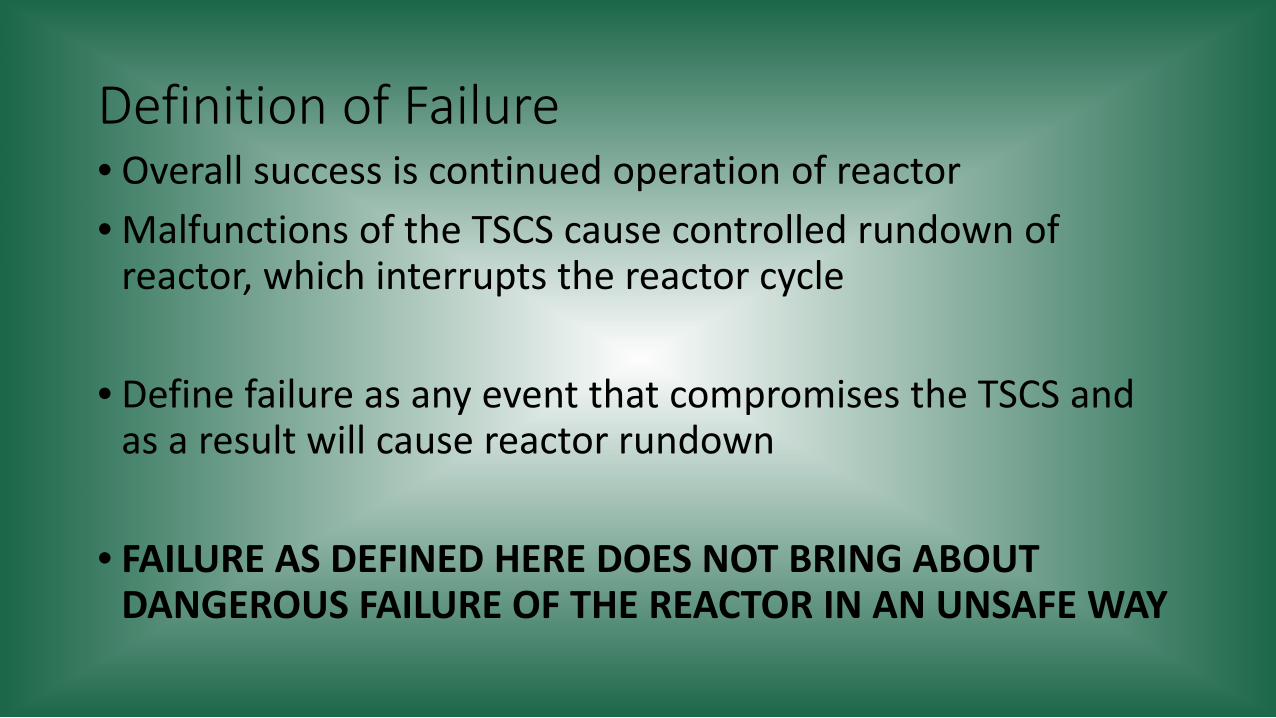
Definition of Failure• Overall success is continued operation of reactor• Malfunctions of the TSCS cause controlled rundown of
reactor, which interrupts the reactor cycle
• Define failure as any event that compromises the TSCS and as a result will cause reactor rundown
• FAILURE AS DEFINED HERE DOES NOT BRING ABOUT DANGEROUS FAILURE OF THE REACTOR IN AN UNSAFE WAY

Failure Modes
• Built-in alarms at set point• Use these events to define main failure modes • Examples: High pressure in supply headers, low flow in
cooling lines• PLC failure
• Structural components (wires, pipes etc) fail much less

Failure Modes and Effects Analysis (FMEA)
• An FMEA lists effects and potential resolution of each failure mode
Portion of B3 Process Area and PLC FMEAs

Markov Diagrams
• A Markov diagram is made for each system component• Nodes are possible states for the component • Connections are transitions between states and have
associated probabilities
Markov diagram for C100 PLCs
Markov diagram for a pressure valve

Markov Diagrams (cont.)
• Time is divided into discrete steps of size Δt. • Δt = 1 day• Transitions can only occur at integer values of Δt
• The total number of component states is related to computation cost.
• TSCS contains M = 19 components and N = 217*3*4 = 1,572,864 states
• The mean time between failures (MTBF) must be known for each component that is modeled

Transition Probabilities • Sum of the probabilities leaving each node must be 1
• The probability that a component operates for time t is:
𝑅𝑅 𝑡𝑡 = 𝑒𝑒−𝑡𝑡
𝑀𝑀𝑀𝑀𝑀𝑀𝑀𝑀
• Therefore, the probability of a component failing within t is:
𝑃𝑃 𝑡𝑡 = 1 − 𝑅𝑅 𝑡𝑡= 1 − 𝑒𝑒−
𝑡𝑡𝑀𝑀𝑀𝑀𝑀𝑀𝑀𝑀
Markov diagram for a pressure valve

Component Transition Probability Matrix
• Let n and n’ be combinations of the states of all 19 components. For element h(n,n’):The transition probability is:
ℎ 𝑛𝑛,𝑛𝑛′ = �𝑖𝑖=1
𝑖𝑖=19
𝑐𝑐𝑖𝑖(𝑛𝑛𝑖𝑖 → 𝑛𝑛′𝑖𝑖)
which is the product of the probabilities of component imaking the transition from ni to ni’

Cell-to-Cell Mapping Technique (CCMT)
• Model evolution of the system’s controlled variables
• System evolves in a controlled variable state space (CVSS) which is partitioned into cells. Each cell, Vj, is a unique combination of control variables
• Alarmed variables that are main failure modes are sink cells; when the system reaches a sink cell, it can no longer evolve
• Cell-to-cell transition probability matrix is made; this matrix is similar to the component transition probability matrix

The Controlled Variable State Space
• Each of alarmed variables is included in the CVSS• 18 controlled variables
Partitions of CVSS for lower supply header flow and T-100 pH

Cell-to-Cell Transition Probabilities
• Transition probabilities between cells Vj and Vj’ will be made into a cell-to-cell transition matrix with elements g(j,j’)
• Program will be written to implement a quadrature scheme
• Stochastic evolution occurs in accordance to the control laws of the system which can be taken from the reactor’s control algorithm

Overall Transition Matrix
• Each element represents a transition between both component states and controlled variable states (n, n’, j, and j’)• q(n,n’,j,j’) = h(n,n’)g(j,j’)
• Matrix can be time dependent if any of the control laws introduce time dependence

Dynamic Event Trees (DETs)
• Choose to start in a state where all components are operational and controlled variables are in an acceptable range
• Tree steps through time and at each time step all possible states are considered using overall transition matrix probabilities
• Use DET generation software (ADAPT, RAVEN) and the transition matrix
Example DET for simplified system over two time steps

Future Goals
• Generate DETs• Determine the CDF and PDF functions for the top events from the DET
software
• OVERALL GOAL: have a working reliability model of the whole system so that individual parts can be switched out to examine the effects of potential system upgrades on reliability

Acknowledgements
• NIST and the SURF program• CHRNS and the NSF• Dr. Dagistan Sahin • Dr. Julie Borchers