Dynamic Programming under Certainty

Sergio Feijoo-Moreira∗

(based on Matthias Kredler’s lectures)

Universidad Carlos III de Madrid

This version: February 15, 2021

Latest version

Abstract

These are notes that I took from the course Macroeconomics II at UC3M, taught

by Matthias Kredler during the Spring semester of 2016. These notes closely follow

Stokey et al. (1989). Typos and errors are possible, and are my sole responsibility

and not that of the instructor.1

Contents

1 Finite Horizon Problems 2

1.1 Introduction . . . . . . . . . . . . . . . . . . . . . . . . . . . . . . . . . . . 2

1.2 The Lagrangian approach . . . . . . . . . . . . . . . . . . . . . . . . . . . 3

1.3 The Dynamic Programming approach . . . . . . . . . . . . . . . . . . . . . 5

1.3.1 Example of Dynamic Programming: McCall Search Model . . . . . 11

2 Infinite Horizon Problems 14

2.1 One-Sector Neo-Classical Growth Model . . . . . . . . . . . . . . . . . . . 14

2.1.1 The Lagrangian approach and transversality conditions . . . . . . . 16

2.1.2 The Dynamic Programming approach . . . . . . . . . . . . . . . . . 19

∗Address: Universidad Carlos III de Madrid. Department of Economics, Calle Madrid 126, 28903

Getafe, Spain. E-mail: sfeijoo@eco.uc3m.es. Web: https://sergiofeijoo.github.io.1This also applies to Fabrizio Leone, very good economist, and even much better friend, who has also

contributed to some parts of these notes.

1

2.2 Mathematical Part: Dynamic Programming . . . . . . . . . . . . . . . . . 22

2.2.1 A function space for V . . . . . . . . . . . . . . . . . . . . . . . . . 22

2.2.2 T is a Contraction Mapping . . . . . . . . . . . . . . . . . . . . . . 24

2.2.3 T is a Self-Mapping . . . . . . . . . . . . . . . . . . . . . . . . . . . 26

2.3 Principle of Optimality . . . . . . . . . . . . . . . . . . . . . . . . . . . . . 28

2.4 Bellman equations . . . . . . . . . . . . . . . . . . . . . . . . . . . . . . . 35

References 39

A Appendix: Envelope Theorem 41

1 Finite Horizon Problems

1.1 Introduction

We start with the standard life-cycle consumption-savings problem. There is a unique

agent who is born with some wealth, and in each period can decide to consume some of

her wealth or save it to consume it in the future. If she decides to save it, we assume

that there exists a risk-free mechanism to save assets at a gross return R. We also assume

that this consumer receives an exogenous sequence of earnings in each period. Besides,

the consumer may be borrowing constrained in some periods, according to an exogenous

sequence of borrowing limits. The main components of this model are:

• Time is discrete and finite: t P t0, 1, . . . , T u.

• tωtuTt“0: exogenous deterministic sequence of earnings,

• ct: consumption at time t,

• at: assets (or wealth) coming into period t,

– a0 ě 0 given,

– at`1 ě a¯t`1 for t “ 0, 1, . . . , T ´ 1, where ta

¯tuT`1t“1 , a

¯tď 0, @t, is an exogenous

deterministic sequence of borrowing limits. Besides a¯T`1 “ 0, thus aT`1 ě 0

implies that the agents must die with zero debt.

– Savings yields gross return R from period t to t` 1.

• Budget constraint at time t:

at`1 ď Rpat ` ωt ´ ctq, for t “ 0, . . . , T,

2

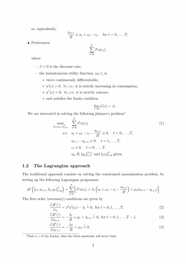
or, equivalently,at`1

Rď at ` ωt ´ ct, for t “ 0, . . . , T,

• Preferences:Tÿ

t“0

βtupctq,

where

– β ą 0 is the discount rate,

– the instantaneous utility function, utp¨q, is

∗ twice continuously differentiable,

∗ u1pcq ą 0, @c, i.e. it is strictly increasing in consumption,

∗ u2pcq ă 0, @c, i.e. it is strictly concave,

∗ and satisfies the Inada condition

limcÑ0

u1pcq “ 8.

We are interested in solving the following planner’s problem2

maxtct,at`1u

Tt“0

Tÿ

t“0

βtupctq (1)

s.t. at ` ωt ´ ct ´at`1

Rě 0, t “ 0, . . . , T,

at`1 ´ a¯t`1 ě 0, t “ 1, . . . , T,

ct ě 0, t “ 0, . . . , T,

a0, R, ta¯tuT`1t“1 and tωtu

Tt“0 given.

1.2 The Lagrangian approach

The traditional approach consists on solving the constrained maximization problem, by

setting up the following Lagrangian programme

L´

tct, at`1, λt, µtuTt“0

¯

“

Tÿ

t“0

”

βtupctq ` λt

´

at ` ωt ´ ct ´at`1

R

¯

` µtpat`1 ´ a¯t`1q

ı

The first order (necessary) conditions are given by

BL p¨q

Bct“ βtu1pctq ´ λt

!“ 0, for t “ 0, 1, . . . , T, (2)

BL p¨q

Bat`1

“ ´λtR` µt ` λt`1

!“ 0, for t “ 0, 1, . . . , T ´ 1, (3)

BL p¨q

BaT`1

“ ´λTR` µT

!“ 0. (4)

2Note ct ą 0 (by Inada), thus the third constraint will never bind.

3

From (2) we obtain

λt “ βtu1pctq, (5)

and since marginal utility is always positive (by assumption), then we have λt ą 0 for

t “ 0, . . . , T . As a consequence, in equilibrium, the full sequence of budget constraints

hold with equality. Moreover, (4) and (5) also imply

µT “λTR“βT

Ru1pcT q ą 0,

thus the no-borrowing constraint binds at a˚T`1 “ a¯T`1 “ 0, which implies that the agents

won’t save in the last period.

Finally, rewriting (3) yields

λt “ Rpλt`1 ` µtq, (6)

where substituting (5) and re-arranging we obtain

u1pctq “ Rβu1pctq `Rβ´tµt, for t “ 0, 1, . . . , T ´ 1. (7)

Therefore we have:

• If µt “ 0 for some t, then the agent is not constrained by the borrowing limit, i.e.

a˚t`1 ą a¯t`1, and thus we obtain the usual (consumption) Euler equation given by

u1pctq “ Rβu1pct`1q. (8)

This equation tells us that if the consumer is not constrained by the borrowing limit,

to be optimizing the marginal cost of saving (i.e., not eating today one unit of the

consumption good) given by the LHS of the previous equation and measured by

the marginal utility of consuming that unit today, must be equal to the marginal

benefit of saving (i.e., eating tomorrow R units of the consumption good) given by

the RHS of the previous equation and measured by the discounted marginal utility of

consuming R tomorrow. Re-arranging this expression we can obtain a more ‘micro’

interpretation, given byu1pctq

βu1pct`1q“ R,

which tells us that in an interior solution, the MRS between ct and ct`1 must be

equal to their price ratio (relative price between ct and ct`1).

• If µt ą 0 for some t, then the agent is constrained by the borrowing limit, i.e.

a˚t`1 “ a¯t`1, and thus we have

u1pctq ą Rβu1pct`1q,

which tells us that the consumer would like to increase ct even further, but she can’t

as she is borrowing constrained.

4

Special case: No borrowing limit Assume that a¯t“ ´8 for t “ 1, . . . , T , and

aT`1 “ 0. In this case, the borrowing constraint does not bind at any t, which implies

µt “ 0, for t “ 0, 1, . . . , T ´ 1. Given that the budget constraint holds with equality,

substituting it into (8) yields

u1ˆ

a˚t ` wt ´a˚t`1

R

˙

“ u1ˆ

a˚t`1 ` wt`1 ´a˚t`2

R

˙

, for t “, , . . . , T ´ 1,

which is a second order difference equation for ta˚t uT`1t“0 with boundary conditions a˚0 “ a0

and a˚T`1 “ 0.

Digression: Power utility Consider the life-cycle consumption-savings model without

borrowing limits and instantaneous utility function

upctq “c1´γt

1´ γ.

Then, from (8) we obtain the Euler equation

c´γt “ βRc´γt`1 ùñ

ˆ

ctct`1

˙´γ

“ βR,

Taking logs we obtain

ln

ˆ

ct`1

ct

˙

“ln β ` lnR

γ,

where ln ct`1´ ln ct “ ln´

ct`1

ct

¯

is the percentage growth rate of consumption. The inter-

temporal rate of substitution (IRS) is defined as

IRS “

d ln

ˆ

ct`1

ct

˙

d lnR“

1

γ.

1.3 The Dynamic Programming approach

The aim of Dynamic Programming is decomposing a complex problem into many sub-

problems and then solving them with a recursive algorithm. In economics, it is particularly

useful to break the returns of an optimal plan into two parts: the current return and the

discounted continuation return. Such a solution strategy for sequential problems brings

us a mayor advantage, it simplifies the computation required to solve the problem. Before

starting to analyse somehow deeper the features of the dynamic programming approach,

let us state a general notation for this kind of problem. A standard finite sequential

5

maximization problem can written as

V ˚px0q “ suptxt`1u

Tt“0

Tÿ

t“0

βtFtpxt, xt`1q

s.t. xt`1 P Γtpxtq, for t “ 0, 1, . . . , T ´ 1

x0 given

Hereafter, we will refer to this formulation as the sequence problem (SP). We call xt the

state (to be defined below), X is the space such that xt P X, @t; Γtpxtq : X Ñ X is the

set of feasible actions, which we call the feasible set correspondence, and Ftpxt, xt`1q :

X ˆX Ñ R is the return function. The problem above can be read as follows: given an

exogenous initial value x0, in each time period t from 0 to T we need to choose a set of

control variables xt`1 that maximize the return function among all the possible choices

given by the feasible set correspondence. Finally, V ˚px0q is called the value function

and it specifies the highest possible value that the return (objective) function can reach

starting with some xt at time t. Note that we have used the operator ‘sup’ instead of the

operator ‘max’ since, until now, nothing ensures us that the maximum value is attained

by any feasible plan that we can choose. Nevertheless, in almost all the possible economic

applications we can use the operator ‘max’ considering that we do not allow for infinite

returns.

Definition 1.1 (State). The state at time t is the smallest set of variables at t that

allows to

• determine the feasible set for the controls (i.e. Γtpxq),

• determine the current return at t (i.e. Ftpx, x1q) given an x1 P Γtpxq,

• determine the value tomorrow given an x1 P Γpxq.

We can rewrite this problem following a dynamic programming approach as follows.

First note that since time is finite, VT`1pxq “ 0, @x P X, i.e., since the agent dies at time

T , the value perceived by this agent because of saving from T to T ` 1 is 0. For a generic

t, we can write the following functional equation (Bellman equation)

Vtpxq “ supx1PΓtpxq

tFtpx, x1q ` βVt`1px

1qu , (9)

with the following associated policy function

gtpxq “ arg supx1PΓtpxq

tFtpx, x1q ` βVt`1px

1qu ,

6

One immediate question to address is the following, from here, how can we obtain the

Euler equations? For this, we need to use the Envelope theorem! (See Appendix: Envelope

Theorem). Assuming an interior solution, the first order condition of (9) yields

BVtpxq

Bx1“ 0 ô

BFtpx, x1q

Bx1` β

BVt`1px1q

Bx1“ 0, (10)

where by the Envelope theorem we have that

BVt`1pxq

Bx“BFt`1px, x

1q

Bx,

which impliesBVt`1px

1q

Bx1“BFt`1px

1, x2q

Bx1,

Then, substituting in (10) we obtain

BFtpx, x1q

Bx1` β

BFt`1px1, x2q

Bx1“ 0.

Turning to the problem given by (1), we a have a slight complication which is the

presence of a borrowing constraint. We’ll see how to deal with this later. In any case, as

time is finite we can solve this problem backwards:

• At period t “ T (the last period), we know that the agent will not want to die with

positive assets, therefore she will ’eat’ all her capital un period T . Let us define the

following policy function

a1 “ gT paq “ 0.

This equation tells us that the optimal action of the agent at time T is not saving,

i.e. setting aT`1 “ 0. As we can see this function g has a subscript T which

denotes the time period and it is a function of a, the state variable of our problem.

Furthermore, since the optimal choice for T ` 1 is setting a1 “ 0, we can define the

value of the agent of entering period T with assets level a by the following value

function

VT paq “ upcq “ u

ˆ

a` ωT ´a1

R

˙

“ u pa` ωT q ” FT pa, a1“ 0q, (11)

which, loosely speaking, is a function that tell us the level of utility attained by the

agent for each asset level a that she might enter period T with. Note that we are

already imposing that aT`1 “ 0, therefore in period T the agent consumption is

given by both her asset level and her endowment in period T .

• At the remaining periods t “ T ´ 1, T ´ 2, . . . , 1, 0, let us define the return function

as

Ftpa, a1q “ upcq “ u

ˆ

a` ωt ´a1

R

˙

,

7

where a ” at are the assets at the beginning of period T ´ 1 and a1 ” at`1 are

savings for tomorrow. The function Ftp¨q is a function of both assets today and

tomorrow. Let us also define the feasible set correspondence as

Γtpaq “ pa¯t`1, Rpa` ωT´1qs ,

which, again, is a function of the assets today. To be more precise, from now onwards

we define

– State variables: a, ptq, (recall Definition 1.1),

– Control variables: a1.

Loosely speaking, the state variables summarize the state of the economy and the

control variables are the choice variables of each agent at each moment of time.

Once we have defined this we can easily find the value function of entering period t

with assets level a as

Vtpaq “ maxa1PΓtpaq

tFtpa, a1q ` βVt`1pa

1qu ,

with associated policy function

p“ a1q gtpaq “ arg maxa1PΓtpaq

tFtpa, a1q ` βVt`1pa

1qu .

First, to simplify the exposition, suppose that there are no borrowing constraints

(you may assume a¯t“ ´8 for t “ 1, . . . , T , and a

¯T`1 “ 0). In this case the first

order (necessary) conditions are given by

BVtpaq

Ba1“ 0 ðñ

BFtpa, a1q

Ba1` β

BVt`1pa1q

Ba1“ 0, (12)

where by the Envelope theorem we know that

BVt`1paq

Ba“BFt`1pa, a

1q

Ba,

which impliesBVt`1pa

1q

Ba1“BFt`1pa

1, a2q

Ba1,

therefore (12) can be rewritten as

BFtpa, a1q

Ba1` β

BFt`1pa1, a2q

Ba1“ 0.

Substituting the specific expression for the return function we obtain

´1

Ru1ˆ

a` ωt ´a1

R

˙

` β

„

u1ˆ

a1 ` ωt`1 ´a2

R

˙

“ 0,

8

or equally

u1ˆ

a` ωt ´a1

R

˙

“ Rβu1ˆ

a1 ` ωt`1 ´a2

R

˙

,

which can also be expressed as

u1pcq “ Rβu1pc1q.

This is exactly the same result that we obtained with the Lagrangian approach.

However, given that in our setting the consumer can be borrowing constrained, we

have to be careful when using the Envelope theorem. The next proposition deals

with this issue.

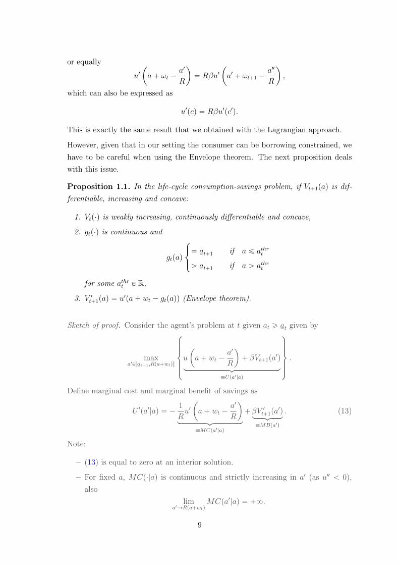
Proposition 1.1. In the life-cycle consumption-savings problem, if Vt`1paq is dif-

ferentiable, increasing and concave:

1. Vtp¨q is weakly increasing, continuously differentiable and concave,

2. gtp¨q is continuous and

gtpaq

$

&

%

“ a¯ t`1 if a ď athrt

ą a¯ t`1 if a ą athrt

for some athrt P R,

3. V 1t`1paq “ u1pa` wt ´ gtpaqq (Envelope theorem).

Sketch of proof. Consider the agent’s problem at t given at ě a¯t

given by

maxa1Pra

¯t`1,Rpa`wtqs

$

’

’

’

&

’

’

’

%

u

ˆ

a` wt ´a1

R

˙

` βVt`1pa1q

looooooooooooooooomooooooooooooooooon

”Upa1|aq

,

/

/

/

.

/

/

/

-

.

Define marginal cost and marginal benefit of savings as

U 1pa1|aq “ ´1

Ru1ˆ

a` wt ´a1

R

˙

looooooooooomooooooooooon

”MCpa1|aq

` βV 1t`1pa1q

loooomoooon

”MBpa1q

. (13)

Note:

– (13) is equal to zero at an interior solution.

– For fixed a, MCp¨|aq is continuous and strictly increasing in a1 (as u2 ă 0),

also

lima1ÑRpa`wtq

MCpa1|aq “ `8.

9

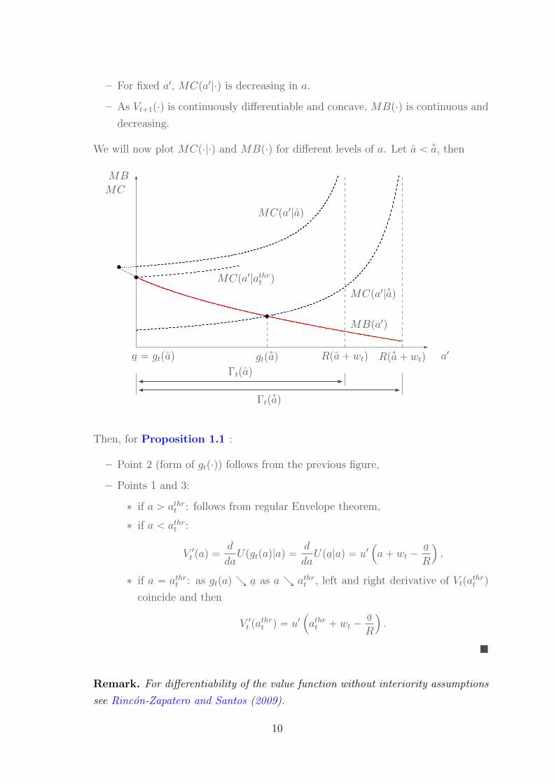
– For fixed a1, MCpa1|¨q is decreasing in a.

– As Vt`1p¨q is continuously differentiable and concave, MBp¨q is continuous and

decreasing.

We will now plot MCp¨|¨q and MBp¨q for different levels of a. Let a ă ˆa, then

a1

MBMC

MCpa1|ˆaq

MCpa1|aq

MCpa1|athrt q

MBpa1q

a¯“ gtpaq gtpˆaq Rpa` wtq Rpˆa` wtq

Γtpaq

Γtpˆaq

Then, for Proposition 1.1 :

– Point 2 (form of gtp¨q) follows from the previous figure,

– Points 1 and 3:

∗ if a ą athrt : follows from regular Envelope theorem,

∗ if a ă athrt :

V 1t paq “d

daUpgtpaq|aq “

d

daUpa

¯|aq “ u1

´

a` wt ´a¯R

¯

,

∗ if a “ athrt : as gtpaq Œ a¯

as a Πathrt , left and right derivative of Vtpathrt q

coincide and then

V 1t pathrt q “ u1

´

athrt ` wt ´a¯R

¯

.

�

Remark. For differentiability of the value function without interiority assumptions

see Rincon-Zapatero and Santos (2009).

10

1.3.1 Example of Dynamic Programming: McCall Search Model

• Real-options problem.

• Dynamic programming also works for solving discrete choice problem (dynamic

choice).

Model:

• Time is finite and discrete: t “ 0, 1.

• There is one agent (a worker). A t “ 0, 1 draws i.i.d wage ωt from a c.d.f. F pωq

with support rω¯, ωs. Decision:

– Accept: stay with ωt until the end,

– Reject: get α in the current period, and have a new draw in the next period.

• yt earnings of the worker.

• Assumption: α P pω¯, ωq.

• Worker maximizes Ery0 ` βy1s, where β P p0, 1q.

To solve this problem, we start by studying the decision of the worker at time t “ 1.

Let V1pωq be the value of having drawn offer ω at t “ 1. Moreover, let V rej1 pωq be the

value of rejecting offer ω at t “ 1 and let V acc1 pωq be the value of accepting offer ω at

t “ 1. In this case we have

V rej1 pωq “ α,

V acc1 pωq “ ω,

V1pωq “ maxtV rej1 pωq, V acc

1 pωqu.

We can represent this value function as

α

ω

V acc1 pωq

V rej1 pωq

α

V1pωq

11

and the policy function at t “ 1 is given by

g1pωq “

$

&

%

1 (Accept) if ω ě α

0 (Reject) if ω ă α(14)

As a consequence, conditional on having rejected the wage drawn in period t “ 0, the

reservation wage in period t “ 1 is just the outside option α.

Now let V0pωq be the value of having drawn offer ω at t “ 0. Moreover, let V rej0 pωq be

the value of rejecting offer ω at t “ 0 and let V acc0 pωq be the value of accepting offer ω at

t “ 0. In this case we have

V rej0 pωq “ α ` E rV1pωqs ,

V acc0 pωq “ ω ` βω,

where

E rV1pωqs “

ż ω

ω¯

V1pω1qdF pω1q

“

ż α

ω¯

αdF pω1q `

ż ω

α

ω1dF pω1q

“ F pαqα `

ż ω

α

ω1dF pω1q.

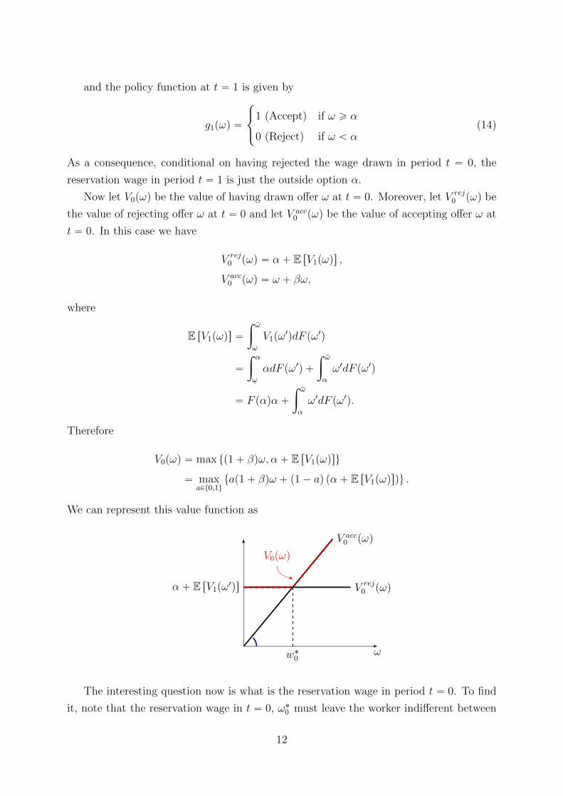
Therefore

V0pωq “ max tp1` βqω, α` E rV1pωqsu

“ maxaPt0,1u

tap1` βqω ` p1´ aq pα ` E rV1pωqsqu .

We can represent this value function as

α ` E rV1pω1qs

ω

V acc0 pωq

V rej0 pωq

w˚0

V0pωq

The interesting question now is what is the reservation wage in period t “ 0. To find

it, note that the reservation wage in t “ 0, ω˚0 must leave the worker indifferent between

12

accepting this wage and sticking with it until the end of period t “ 1 or rejecting it,

obtaining today α and having a new drawn in period t “ 1. This indifference is given by

the equality V rej0 pω˚0 q “ V rej

0 pω˚0 q, which implies

p1` βqω˚0 “ α ` β

„

F pαqα `

ż ω

α

ω1dF pω1q

.

Therefore

ω˚0 “

α ` β

„

F pαqα `

ż ω

α

ω1dF pω1q

1` β.

Intuitively, w˚0 ą α, as α is always available for the worker as an outside option. However,

let us prove it. First note that

E rV1pωqs “ F pαqαloomoon

Obtain α

`

ż ω

α

ω1dF pω1qloooooomoooooon

Obtain ωąα

ą α,

thus

α ` E rV1pωqs ą α ` βα,

and finally this implies that w˚0 ą α “ w˚1 . Consequently, the worker gets less picky over

time (option value of waiting).

13

2 Infinite Horizon Problems

2.1 One-Sector Neo-Classical Growth Model

This is one of the workhorse models of modern macroeconomics. The environment is

given by:

• Large number of identical households:

– Each household starts with k0 units of capital.

– Labour endowment: for every t, the household chooses labour nt P r0, 1s.

• Single consumption good which is produced with only two inputs, capital and labour.

The production function is

yt “ F pkt, ntq,

where F p¨q is a neo-classical production function with the following properties:

– F pk, nq is continuously differentiable.

– Strictly increasing in both arguments, i.e. Fkpk, nq ą 0, Fnpk, nq ą 0, @k, n.

– Strictly concave in both arguments, i.e. Fkkpk, nq ă 0, Fnnpk, nq ă 0, @k, n.

This means that the production function exhibits decreasing marginal returns.

– Constant returns to scale (the production function is homogeneous of degree

1), i.e.,

F pλk, λnq “ λF pk, nq, @λ ą 0.

With this assumption the size of the firm is indeterminate (the model cannot

tell us anything about this).

– Inada conditions:

limkÑ0

Fkpk, 1q “ 8 limnÑ0

Fnp1, nq “ 8

limkÑ8

Fkpk, 1q “ 0 limnÑ8

Fnp1, nq “ 0

– Inputs essential, i.e., F p0, nq “ 0, F pk, 0q “ 0, @k, n.

– Examples:

∗ Cobb Douglas:

F pk, nq “ Akαnp1´αq,

where α P p0, 1q, and A is the total factor productivity.

14

∗ CES (Constant elasticity of substitution):

F pk, nq “ A pµkρ ` p1´ µqnρq1{ρ ,

where typically µ P p0, 1q, ρ ă 1, and A is the total factor productivity.

• Investment:

ct ` kt`1 ď F pk, nq ` p1´ δqkt.

Note that this could be different due to, for example, irreversibilities or the presence

adjustment costs.

• Preferences of the representative household:

U`

tctu8

t“0

˘

“

8ÿ

t“0

βtupctq,

where u1pcq ą 0, u2pcq ă 0 and

limcÑ8

u1pcq “ 8.

Note that in this environment, leisure is not valued. Therefore each household will

allocate all their time to work, i.e. nt “ 1, @t.

We are interested in solving the planner’s problem. In this environment, a planner

will solve

maxtct,kt`1u

8t“0

8ÿ

t“0

βtupctq (15)

s.t. ct ` kt`1 ď F pkt, 1q ` p1´ δqkt t “ 0, 1, . . . ,

ct ě 0, t “ 0, 1, . . . ,

kt`1 ě 0, t “ 0, 1, . . . ,

k0 given.

where we define fpktq as the feasible resources at date t, i.e. fpktq “ F pkt, 1q ` p1´ δqkt.

Note the following:

1. Since u1pctq ą 0, then the feasibility constraint will always hold with equality (we

do not want to leave goods on the table).

2. By the Inada conditions, ct “ 0 can’t be optimal, therefore we must have ct ą 0, @t.

3. If kt`1 “ 0 for some t, then fpkt`1q “ 0. Then we would have that ct`1 “ 0. This

possibility is ruled out, again, by the Inada conditions. Then we must have that

kt`1 ą 0, @t.

15

2.1.1 The Lagrangian approach and transversality conditions

As we did in the finite horizon case, we can solve this problem setting up the following

Lagrangian

L`

tct, kt`1, λtu8

t“0

˘

“

8ÿ

t“0

“

βtupctq ` λt pfpktq ´ ct ´ kt`1q‰

.

The first order necessary conditions for having a maximum are given by

BL p¨q

Bct“ 0 ô βtu1pctq ´ λt “ 0, @t, (16)

BL p¨q

Bkt`1

“ 0 ô ´λt ` λt`1f1pkt`1q “ 0, @t, (17)

Combining (16) and (17) we obtain

u1pctq “ βu1pct`1qf1pkt`1q, @t,

which is the Euler equation with the usual interpretation, in the optimum, the marginal

cost of saving one unit must be equal to the discounted marginal utility of consuming

the return of capital. The Euler equations give us necessary conditions for a solution

c˚t , k˚t`1

(8

t“0. Note that by substituting the feasibility constraint in the Euler equation

we obtain

u1pfpktq ´ kt`1q “ βu1pfpkt`1q ´ kt`2qf1pkt`1q, @t,

which is a second order difference equation for

k˚t`1

(8

t“0. This equation together with

the initial condition k0 “ k˚0 characterize the optimal path of

k˚t`1

(8

t“0, but we are still

lacking a terminal condition, this is where the transversality condition will come in handy.

Up until now, we have found necessary conditions for a solution, but we are interested

in finding sufficient conditions for a solution.

Fact 2.1. Let gp¨q and fp¨q be concave functions, and furthermore, let gp¨q be an increas-

ing function. Then hp¨q “ g pf p¨qq is also a concave function.

Fact 2.2. Let x P Rn and let fpxq be a function f : Rn Ñ R that is differentiable and

concave. Then

fpxq `Dfpxq1rx´ xs ě fpxq,

where

Dfpxq “

»

—

—

–

f1pxq...

fnpxq

fi

ffi

ffi

fl

,

is the gradient of f in the point x.

16

Proposition 2.1. (Guner, 2008, Proposition 77, pp.136-137). Consider

maxtkt`1u

8t“0

8ÿ

t“0

βtF pkt, kt`1q

s.t. kt`1 ě 0, @t,

k0 given.

Let F p¨q be continuously differentiable, and let F px, yq be concave in px, yq and strictly

increasing in x. If the sequence

k˚t`1

(8

t“0satisfies:

• k˚t`1 ě 0, @t;

• (Euler equation): F2pk˚t , k

˚t`1q ` βF1pk

˚t`1, k

˚t`2q “ 0, @t;

• (Transversality Condition): limtÑ8 βtF1pk

˚t , k

˚t`1qk

˚t “ 0;

Then

k˚t`1

(8

t“0maximizes the objective function, that is, the Euler equations are sufficient

for tk˚0 , k˚1 , . . .u to maximize

U pk˚0 , k˚1 , . . .q “

8ÿ

t“0

βtF`

k˚t , k˚t`1

˘

. (18)

Proof. First consider a finite horizon T and rewrite (18) as

U`

k˚0 , k˚1 , ..., k

˚T`1

˘

“ F pk˚0 , k˚1 q ` βF pk

˚1 , k

˚2 q ` β

2F pk˚2 , k˚3 q ` ...` β

TF pk˚T , k˚T`1q,

then we have that

D“

U`

k˚0 , k˚1 , ..., k

˚T`1

˘‰

“

»

—

—

—

—

—

—

—

—

—

–

BU`

k˚0 , k˚1 , ..., k

˚T`1

˘

Bk˚0BU

`

k˚0 , k˚1 , ..., k

˚T`1

˘

Bk˚1...

BU`

k˚0 , k˚1 , ..., k

˚T`1

˘

Bk˚T`1

fi

ffi

ffi

ffi

ffi

ffi

ffi

ffi

ffi

ffi

fl

“

»

—

—

—

—

—

—

—

–

F1pk˚0 , k

˚1 q

F2pk˚0 , k

˚1 q ` βF1pk

˚1 , k

˚2 q

...

βT´1F2pk˚T´1, k

˚T q ` β

TF1pk˚T , k

˚T`1q

βTF2pk˚T , k

˚T`1q

fi

ffi

ffi

ffi

ffi

ffi

ffi

ffi

fl

,

and thus by Fact 2.2 we have

Upk˚1 , ..., k˚T`1q `D

“

U`

k˚0 , k˚1 , ..., k

˚T`1

˘‰1

»

—

—

—

—

—

—

—

–

k0 ´ k˚0

k1 ´ k˚1

...

kT ´ k˚T

kT`1 ´ k˚T`1

fi

ffi

ffi

ffi

ffi

ffi

ffi

ffi

fl

ě Upk1, ..., kT`1q. (19)

17

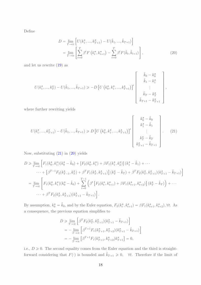
Define

D “ limTÑ8

”

Upk˚1 , ..., k˚T`1q ´ Upk1, ..., kT`1q

ı

“ limTÑ8

«

Tÿ

t“0

βtF`

k˚t , k˚t`1

˘

´

Tÿ

t“0

βtF pkt, kt`1q

ff

, (20)

and let us rewrite (19) as

Upk˚1 , ..., k˚T q ´ Upk1, ..., kT`1q ě ´D

“

U`

k˚0 , k˚1 , ..., k

˚T`1

˘‰1

»

—

—

—

—

—

—

—

–

k0 ´ k˚0

k1 ´ k˚1

...

kT ´ k˚T

kT`1 ´ k˚T`1

fi

ffi

ffi

ffi

ffi

ffi

ffi

ffi

fl

,

where further rewriting yields

Upk˚1 , ..., k˚T`1q ´ Upk1, ..., kT`1q ě D

“

U`

k˚0 , k˚1 , ..., k

˚T`1

˘‰1

»

—

—

—

—

—

—

—

–

k˚0 ´ k0

k˚1 ´ k1

...

k˚T ´ kT

k˚T`1 ´ kT`1

fi

ffi

ffi

ffi

ffi

ffi

ffi

ffi

fl

. (21)

Now, substituting (21) in (20) yields

D ě limTÑ8

”

F1pk˚0 , k

˚1 qpk

˚0 ´ k0q ` rF2pk

˚0 , k

˚1 q ` βF1pk

˚1 , k

˚2 qs pk

˚1 ´ k1q ` ¨ ¨ ¨

¨ ¨ ¨ `“

βT´1F2pk˚T´1, k

˚T q ` β

TF1pk˚T , k

˚T`1q

‰

pk˚T ´ kT q ` βTF2pk

˚T , k

˚T`1qpk

˚T`1 ´ kT`1q

ı

“ limTÑ8

«

F1pk˚0 , k

˚1 qpk

˚0 ´ k0q `

T´1ÿ

t“0

´

βt“

F2pk˚t , k

˚t`1q ` βF1pk

˚t`1, k

˚t`2q

‰

pk˚T ´ kT q¯

` ¨ ¨ ¨

¨ ¨ ¨ ` βTF2pk˚T , k

˚T`1qpk

˚T`1 ´ kT`1q

ı

.

By assumption, k˚0 “ k0, and by the Euler equation, F2pk˚t , k

˚t`1q “ βF1pk

˚t`1, k

˚t`2q, @t. As

a consequence, the previous equation simplifies to

D ě limTÑ8

”

βTF2pk˚T , k

˚T`1qpk

˚T`1 ´ kT`1q

ı

“ ´ limTÑ8

”

βT`1F1pk˚T`1, k

˚T`2qpk

˚T`1 ´ kT`1q

ı

“ ´ limTÑ8

“

βT`1F1pk˚T`1, k

˚T`2qk

˚T`1

‰

“ 0,

i.e., D ě 0. The second equality comes from the Euler equation and the third is straight-

forward considering that F p¨q is bounded and kT`1 ě 0, @t. Therefore if the limit of

18

the previous expression is 0, or in other words, if the transversality condition is satisfied,

then tk˚t`1u8t“0 maximizes the objective function.

Note that the transversality condition can be also be written by going one period

backwards, obtaining

limTÑ8

“

βTF1pk˚T , k

˚T`1qk

˚T

‰

“ 0. (22)

�

2.1.2 The Dynamic Programming approach

The problem (15) can be rewritten as the following sequential problem

maxtkt`1u

8t“0

8ÿ

t“0

βtupfpktq ´ kt`1q (23)

s.t. kt`1 P Γpktq “ r0, fpktqs , t “ 0, 1, . . .

k0 given.

Note that as we have moved to infinite time, we can get rid of the time subscript of the

feasibility correspondence. Why we can do this? This follows from the idea of recursion

that we will exploit to solve this problem. As time is infinite, the world must look exactly

the same today and tomorrow. This idea of recursion allows us to split problem into two

parts, today and the entire future. To better understand this approach, note that we can

rewrite (23) as

maxtkt`1u

8t“0

k0 given

8ÿ

t“0

βtupfpktq ´ kt`1q

s.t. kt`1PΓpktq

“ maxk1PΓpk1qk0 given

upfpk0q ´ k1q

looooooooooooomooooooooooooon

Today

` maxtkt`1u

8t“1

k1 given

8ÿ

t“1

βtupfpktq ´ kt`1q

s.t. kt`1PΓpktqlooooooooooooooooooomooooooooooooooooooon

Future

“ maxk1PΓpk1qk0 given

upfpk0q ´ k1q ` β maxtkt`1u

8t“1

k1 given

8ÿ

t“1

βt´1upfpktq ´ kt`1q

s.t. kt`1PΓpktq

“ maxk1PΓpk1qk0 given

upfpk0q ´ k1q ` β maxtkt`1u

8t“1

k1 given

8ÿ

t“0

βtupfpkt`1q ´ kt`2q

s.t. kt`2PΓpkt`1q

.

Let us define the maximized value of the problem given k0 as

V pk0q “ maxtkt`1u

8t“0

k0 given

8ÿ

t“0

βtupfpktq ´ kt`1q

s.t. kt`1PΓpktq

,

19

then we can write

V pk0q “ maxk1PΓpk0q

tupfpk0q ´ k1q ` βV pk1qu .

As time is infinite, we can write the value function for a generic t as

V pkq “ maxk1PΓpkq

tupfpkq ´ k1q ` βV pk1qu , (24)

where it is important to remark that the time subscript is no longer relevant. Besides, we

can define the optimal policy function as

gpkq “ arg maxk1PΓpkq

tupfpkq ´ k1q ` βV pk1qu (25)

In the dynamic programming approach, instead of looking for the optimal sequence

tkt`1u8

t“0 like we do in the lagrangian (or sequential) approach, we will look for a pair of

functions V p¨q and gp¨q.

There are some open questions that we would like to answer:

• Is V pkq well defined? The answer is yes as long as we replace the max operator for

the sup operator (the max may not exist, but the supremum is always well defined).

Let us redefine the problem with a sup operator

V pk0q ” suptkt`1u

8t“0

8ÿ

t“0

βtupfpktq ´ kt`1q (SP)

s.t. kt`1 P Γpktq “ r0, fpktqs , t “ 0, 1, . . . ,

k0 given.

• Is any solution V p¨q to the functional equation

V pkq “ sup0ďk1ďfpkq

!

upfpkq ´ k1q ` βV pk1q)

(FE)

equal to V p¨q, i.e. V pkq “ V pkq, @k ě 0 and gives us the correct maximizing

sequence to the sequence problem (SP)? In other words, will a solution to the

Functional equation (Bellman equation) be unique? Will it be the same solution as

the one obtained from the Sequential Problem?

• If the answer to the previous question is yes, how we can find a solution to the

Functional equation (Bellman equation) (FE)? In functional equations the unknowns

are precisely functions, therefore we need to define the space in which we want to

look for the function that solves our functional equation. In our case, we will look

for a solution in the space of continuous and bounded functions.

20

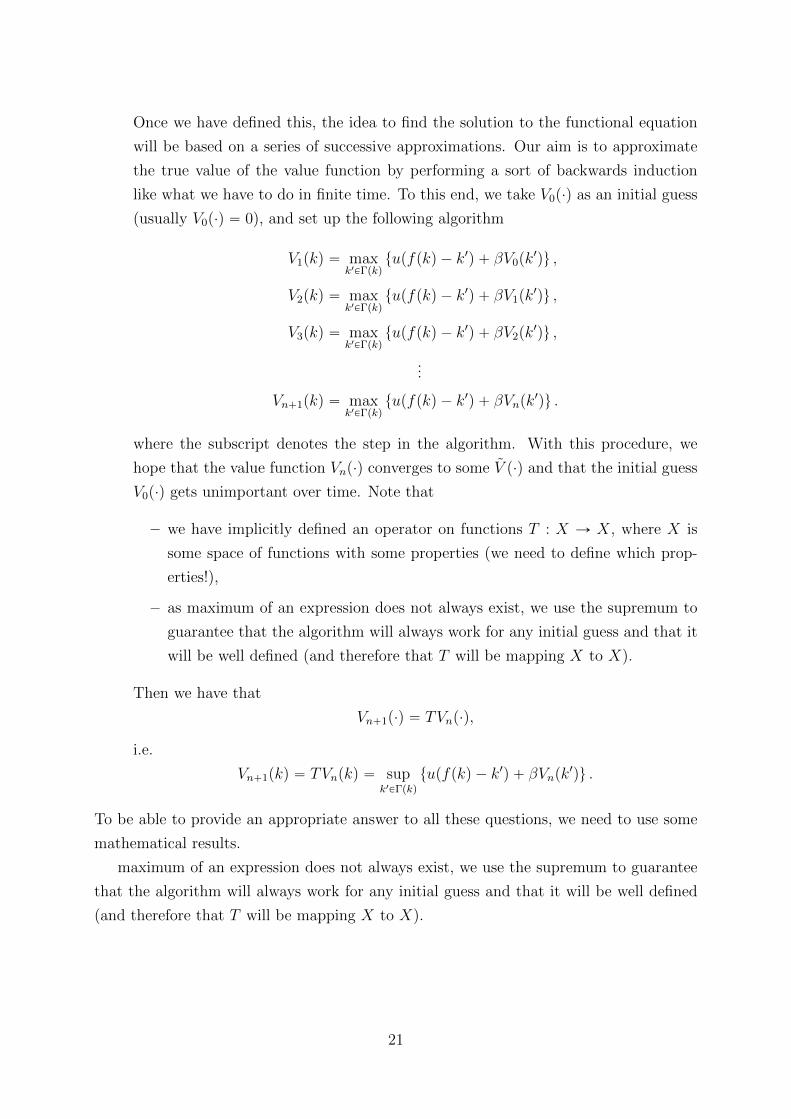
Once we have defined this, the idea to find the solution to the functional equation

will be based on a series of successive approximations. Our aim is to approximate

the true value of the value function by performing a sort of backwards induction

like what we have to do in finite time. To this end, we take V0p¨q as an initial guess

(usually V0p¨q “ 0), and set up the following algorithm

V1pkq “ maxk1PΓpkq

tupfpkq ´ k1q ` βV0pk1qu ,

V2pkq “ maxk1PΓpkq

tupfpkq ´ k1q ` βV1pk1qu ,

V3pkq “ maxk1PΓpkq

tupfpkq ´ k1q ` βV2pk1qu ,

...

Vn`1pkq “ maxk1PΓpkq

tupfpkq ´ k1q ` βVnpk1qu .

where the subscript denotes the step in the algorithm. With this procedure, we

hope that the value function Vnp¨q converges to some V p¨q and that the initial guess

V0p¨q gets unimportant over time. Note that

– we have implicitly defined an operator on functions T : X Ñ X, where X is

some space of functions with some properties (we need to define which prop-

erties!),

– as maximum of an expression does not always exist, we use the supremum to

guarantee that the algorithm will always work for any initial guess and that it

will be well defined (and therefore that T will be mapping X to X).

Then we have that

Vn`1p¨q “ TVnp¨q,

i.e.

Vn`1pkq “ TVnpkq “ supk1PΓpkq

tupfpkq ´ k1q ` βVnpk1qu .

To be able to provide an appropriate answer to all these questions, we need to use some

mathematical results.

maximum of an expression does not always exist, we use the supremum to guarantee

that the algorithm will always work for any initial guess and that it will be well defined

(and therefore that T will be mapping X to X).

21

2.2 Mathematical Part: Dynamic Programming

Let us redefine the problem given by (15) with a more general notation. Consider the

sequence problem (SP) approach given by

V ˚px0q “ suptxt`1u

8t“0

8ÿ

t“0

βtF pxt, xt`1q (SP)

s.t. xt`1 P Γpxtq, for t “ 0, 1, . . . ,

x0 given.

The dynamic programming approach to this problem is given by the Functional equation

(Bellman equation)

V pxq “ supx1PΓpxq

F px, x1q ` βV px1q. (FE)

which implicitly defines an operator T given by

T : pTV qpxq “ supx1PΓpxq

tF px, x1q ` βV px1qu ,

read as : Vn`1pxq “ supx1PΓpxq

tF px, x1q ` βVnpx1qu .

We will now focus on the properties of the Bellman equation in an infinite time setting.

The first difference to be noted relies on the absence of an explicit final condition of the

form VT`1 “ 0. We are interested in studying under which conditions this recursive

problem is well defined and actually admits a (unique) solution. To this end, we will

follow the next steps:

1. Define a function space for V ,

2. Show that T is a contraction mappings,

3. Show that T is a self-mapping,

4. The Principle of Optimality (SP ô FE).

2.2.1 A function space for V

Let us introduce some mathematical definitions that we will need.3

Definition 2.1 (Metric). A metric or distance function on X is a function d : XˆX Ñ

R` such that for every x, y, z P X we have

3Unless stated otherwise, all the definitions and theorems that you’ll find until Section 2.3 have been

obtained from the lecture notes of the Mathematics course taught by Juan Pablo Rincon-Zapatero (n.d.).

You may go back to his notes for a detailed and clearer explanation, proofs and/or examples.

22

(i) dpx, yq ě 0,

(ii) dpx, yq “ 0 ô x “ y,

(iii) dpx, yq “ dpy, xq,

(iv) Triangle inequality: dpx, zq ď dpx, yq ` dpy, zq.

Definition 2.2 (Metric Space). A Metric Space is pair pX, dq, where X is a set and d

is a metric defined on it.

Some sets X have an algebraic structure that allows us to operate with their elements.

In particular we will consider vector spaces. We are interested not only in measuring the

distance between points, but also in giving a meaning to the length of a vector.

Definition 2.3 (Vector Space). A vector space X is a set that is closed under finite

vector addition and scalar multiplication. Let f, g P X, then

• Addition: pf ` gqpxq “ fpxq ` gpxq,

• Scalar Multiplication: pλfqpxq “ λfpxq.

Definition 2.4 (Norm). Let X be a vector space over the reals (hence, in particular,

0 P X). A norm on X is a function ‖¨‖ : X Ñ R` such that for every x, y P X and for

every scalar λ P R we have

(i) ‖x‖ ě 0,

(ii) ‖x‖ “ 0 ô x “ 0,

(iii) Triangle inequality: ‖x` y‖ ď ‖x‖` ‖y‖,

(iv) Homogeneity: ‖λx‖ “ |λ|‖x‖.

Definition 2.5 (Normed Vector Space). A normed space is a pair pX, ‖¨‖q where X

is a vector space and ‖¨‖ is a norm.

Definition 2.6. Given a set X, the vector space of real bounded and continuous functions

f on X, is denoted CpXq

CpXq “ tf : X Ñ R : f bounded and continuousu .

Definition 2.7 (Supremum Norm). Let X be a set and let CpXq be the space of all

bounded and continuous functions defined on X. The supremum norm is the norm defined

on CpXq by

||f ||8 “ suppxPXq

|fpxq|.

23

Remark. pCpXq, || ¨ ||8q is a normed vector space.

Definition 2.8 (Bolzano-Weirstrass Property). A subset A of a metric space X has

the Bolzano-Weierstrass Property if every sequence in A has a convergent subsequence,

i.e. has a subsequence that converges to a point in A.

Theorem 2.1 (Compact Metric Space). A subset of a metric space is compact if and

only if it enjoys the Bolzano-Weierstrass Property.

Definition 2.9 (Cauchy Sequence). Let pX, dq be a metric space. A sequence xn P X

is Cauchy if given any ε ą 0, there exists n0pεq such that

dpxp, xqq ă ε whenever p, q ě n0pεq.

Remark. Every convergent sequence is a Cauchy sequence, but the reciprocal is not true.

Definition 2.10 (Complete Metric Space). A metric space pX, dq is complete if every

Cauchy sequence converges.

Definition 2.11 (Banach Space). A normed space pX, || ¨ ||q is a Banach Space if it is

complete.

Lemma 2.1. The space CpXq is complete, therefore it is a Banach Space.

We will look for the function V in CpXq, the space of continuous and bounded functions

with the supremum norm. This vector space is a complete normed vector space, and

therefore it is a Banach space.

2.2.2 T is a Contraction Mapping

It turns out that under some regularity conditions, the operator T is a contraction map-

ping. Since we are looking for our function in a Banach space, then if we can show that T

is a contraction mapping we can apply the Banach Fixed Point theorem, that ensures the

existence and uniqueness of the limit function V and also provides and algorithm to find

it. To be able to prove that T is a contraction mapping, we will use Blackwell’s sufficient

conditions.

Definition 2.12 (Mapping). A map is a way of associating unique objects to every

element in a given set. So a map f : A Ñ B from A to B is a function f such that for

every a P A, there is a unique object b P B.

Definition 2.13 (Fixed Point). Let T : X Ñ X be a mapping. We say that x P X is a

fixed point of T if T pxq “ x.

24

Definition 2.14 (Contraction Mapping). Let pX, dq be a metric space. The operator

T : pX, dq Ñ pX, dq is a contraction mapping with parameter (modulus) β if for some

0 ă β ă 1 we have that

dpTx, Tyq ď βdpx, yq, @x, y P X.

Theorem 2.2 (Banach Fixed Point Theorem - Contraction Mapping Theorem).

Let pX, dq be a complete metric space and let T a contraction operator. Then T admits a

unique fixed point, which can be approached from successive iterations of the operator T

from any initial element x P X. In particular, if the contraction parameter is β, then we

have that

• T has exactly one fixed point V P X, i.e. T pV q “ V ,

• and for any V0 P X,

dpT nV0, V q ď βndpV0, V q, n “ 0, 1, . . .

Corollary 2.1. Let pX, ‖¨‖q be a Banach Space and T : pX, ‖¨‖q Ñ pX, ‖¨‖q be a contrac-

tion mapping with fixed point V P X. If X 1 is a closed subset of X and T pX 1q Ď X 1, then

V P X 1. If, in addition, T pE 1q Ď E2 Ď E 1, then V P E2

Proof. Choose V0 P X1. Then the sequence tT nV u8n“0 Ñ V , T nV P X 1. Since E 1 is closed,

V P X 1(by the definition of closeness). If also T pEq Ď X2,then since V “ T pV qand

V P X 1, then T pV q P X2 and thus V P X2. �

How can we identify that some operator T is a contraction? We can show it either by

first principles (i.e., applying the previous mathematical artillery) or we can use Black-

well’s sufficient conditions.

Theorem 2.3 (Blackwell’s Sufficient Conditions). Let X Ă R` and BpXq be the

space of bounded functions f : X Ñ R with the supremum norm. Let T : BpXq Ñ BpXq

be an operator satisfying

1. Monotonicity: if f, g P BpXq and fpxq ď gpxq, @x P X, then this implies that

pTfqpxq ď pTgqpxq, @x P X.

2. Discounting: D some β P p0, 1q such that

rpT pf ` aqs pxq ď pTfqpxq ` βa, @f P BpXq, @a P R`, @x P X.

Then T is a contraction operator with contraction parameter (modulus) β.

25

Example Let us apply this procedure to see whether our operator in the growth model

is a contraction mapping. From (24), write

pTV qpkq “ maxk1PΓpkq

tupfpkq ´ k1q ` βV pk1qu ,

First, let W pkq ě V pkq, @k, then

pTW qpkq “ max0ďk1ďfpkq

tupfpkq ´ k1q ` βW pk1qu

ě max0ďk1ďfpkq

tupfpkq ´ k1q ` βV pk1qu “ pTV qpkq,

as for each 0 ď k1 ď fpkq (for fixed k), and W pk1q ě V pk1q by assumption. Note that

fixing k implies that the feasibility constraint does not change. Therefore, monotonicity

holds in the neoclassical growth model.

Furthermore

rT pV ` aqspkq “ max0ďk1ďfpkq

tupfpkq ´ k1q ` βrV pk1q ` asu

“ max0ďk1ďfpkq

tupfpkq ´ k1q ` βV pk1q ` βau

“ max0ďk1ďfpkq

tupfpkq ´ k1q ` βV pk1qu ` βa,

“ pTV qpkq ` βa

and as “ implies ď, then discounting also holds in the neoclassical growth model.

Therefore, T is a contraction operator in the neoclassical growth model.

2.2.3 T is a Self-Mapping

We want to show that T is a self mapping because if this holds and our initial guess

V0 is, for example, a continuous and bounded function, then T will map continuous and

bounded functions into continuous and bounded functions, and therefore V , our main

interest, will also be a continuous and bounded function. To be able to show that T is a

self-mapping, we will use Berge’s Maximun Theorem. Let us first introduce two relevant

theorems.

Theorem 2.4 (Weierstrass’ Theorem). If f : X Ñ G is a continuous function that

maps a compact metric space X into a metric space G, then fpXq is compact.

Theorem 2.5 (Extreme Value Theorem). Let K be a compact subset of the metric

space X and f : K Ñ R a continuous function. Then there exists x1, x2 P K such that

fpx2q ď fpxq ď fpx1q, @x P K. (26)

26

Now, consider the general problem

vpxq “ supyPΓpxq

fpx, yq,

where x P X, X Ă R`, y P Y , Y Ă Rm, f : XˆY Ñ R and Γ : X Ñ Y . Note that if fpx, ¨q

is continuous in y (for fixed x) and Γ is a non-empty and compact valued correspondence

(i.e. Γpxq is a compact set @x P X), then by fixing an x we are maximizing a continuous

function on a compact set. Then, by Weierstrass’ Theorem (Extreme Value Theorem),

the maximum exists. Let us write the value function hpxq as

hpxq “ maxyPΓpxq

fpx, yq,

and the optimal correspondence (policy function) Gpxq as

Gpxq “ arg maxyPΓpxq

fpx, yq “ ty P Γpxq : fpx, yq “ hpxqu .

Theorem 2.6 (Theorem of the Maximum of Berge). Assume that vpxq ă `8,

@x P X. Then

1. If f is lower semi-continuous and Γ is non-empty and lower hemi-continuous, then

hpxq is lower-semi-continuous.

2. If f is upper semi-continuous and Γ is non-empty, compact-valued and upper hemi-

continuous, then hpxq is upper-semi-continuous.

3. If f is continuous and Γ is non-empty, compact-valued and continuous, then hpxq is

continuous and Gpxq is non-empty, compact-valued and upper hemi-continuous (we

lose lower hemi-continuity).

Corollary 2.2 (Convex Theorem of the Maximum). Suppose that X Ă Rm is

convex, f : X ˆ Y Ñ R is continuous and concave in y (for fixed x) and that Γ : X Ñ Y

is a continuous set-valued mapping, compact valued and with convex graph.Then

1. The value function hpxq is concave and the optimal correspondence Gpxq is convex-

valued.

2. If fpx, ¨q is strictly concave in y for every x P X, then Gpxq is single-valued and it

is continuous as a function.

Remark. We can use as a fact that any correspondence Γpxq “ rfpxq, gpxqs in which the

bounds fpq and gpq are continuous functions is continuous.

27

Example Let us apply this to the one-sector neo-classical growth model. Define

• fpx, yq ” upfpkq´k1q`βV pk1q. Since both up¨q and fp¨q are continuous functions, as

long as V p¨q is a continuous function then upfpkq´k1q`βV pk1q is also a continuous

function.

• Γpkq “ r0, fpkqs. Since 0 and fpxq are both continuous functions of x, then Γpxq is

a non-empty, compact and continuous correspondence.

Then by Berge’s maximum theorem, we have that TV p¨q is a continuous function.

2.3 Principle of Optimality

The value function V ˚px0q given by (SP) tells us the infinite discounted value of following

the best sequence

x˚t`1

(8

t“0. Our hope is that, rather than finding the best sequence

x˚t`1

(8

t“0, we can try to find the function V ˚px0q as a solution to (FE). If our conjecture

is correct, then the function V that solves (FE) would give us the value function, i.e.

V px0q “ V ˚px0q. In this section we will cover some theorems on the relationship between

the sequence problem and the functional equation approach. Let us recover the definition

for the value function V ˚p¨q for the sequence problem, which is given by

V ˚px0q “ suptxt`1u

8t“0

8ÿ

t“0

βtF pxt, xt`1q (SP)

s.t. xt`1 P Γpxtq, @t,

x0 P X given,

where β ě 0, and the dynamic programming approach to this problem is given by the

functional equation (Bellman equation)

V pxq “ supx1PΓpxq

tF px, x1q ` βV px1qu, @x P X. (FE)

Note that we use the sup rather than the max so that we can briefly ignore for the moment

whether the optimum is indeed attained. In this section we will show that

• The value function V ˚p¨q satisfies (FE).

• If there exists a solution to (FE), then it is the value function V ˚p¨q.

• There is indeed a solution to (FE).

• A sequence

x˚t`1

(8

t“0attains the maximum in (SP) if it satisfies

V px˚t q “ F px˚t , x˚t`1q ` βV px

˚t`1q, @t.

28

Before we start, let us set some notation and useful definitions:

• Let X be the set of possible values for the state variable xt.

• ‘Plan’: any sequence txt`1u8

t“0,

• ‘Feasible plan’: plan txt`1u8

t“0 that satisfies xt`1 P Γpxtq for t “ 0, 1, . . .

• Πpx0q: the set of feasible plans given a particular x0, i.e.

Πpx0q “

txt`1u8

t“0 : xt`1 P Γpxtq for t “ 0, 1, . . .(

• x “ tx1, x2, . . .u P Πpx0q is a typical feasible plan.

• For each n “ 0, 1, . . . we will define

unpxq “nÿ

t“0

βtF pxt, xt`1q,

as the discounted return from following a feasible plan x from date 0 to date n.

• Let u : Πpx0q Ñ R

upxq “ limnÑ8

unpxq “ limnÑ8

nÿ

t“0

βtF pxt, xt`1q “

8ÿ

t“0

βtF pxt, xt`1q,

be the infinite discounted sum of returns from following feasible plan x.

The following assumptions impose conditions under which (SP) is well defined.

Assumption (A1). Γpxq ‰ H, @x P X, i.e., there is always at least one feasible sequence.

Assumption (A2). F : A Ñ R is bounded, where A “ tpx, yq : x P X, y P Γpxqu is the

graph of Γp¨q.

Under A1 and A2 the set of feasible plans Πpx0q is non empty for each x0 P X and

(SP) is well defined for every x P Πpx0q. We can then define the supremum function as

V ˚px0q “ supxPΠpx0q

upxq,

i.e., V ˚px0q is the supremum in (SP). Note that as V ˚px0q is a supremum, it is the unique

function that satisfies

V ˚px0q ě upxq, @x P Πpx0q, (SP1)

and for any ε ą 0

V ˚px0q ď upxq ` ε, for some x P Πpx0q. (SP2)

29

This implies that no other feasible sequence can do better than V ˚p¨q, but we can get ε

close, as close as we want. Moreover, V ˚px0q satisfies (FE) if

V ˚px0q ě F px0, yq ` βV˚pyq, @y P Γpx0q, @x0 P X, (FE1)

and for any ε ą 0

V ˚px0q ď F px0, yq ` βV˚pyq ` ε for some y P Γpx0q, @x0 P X, (FE2)

which has the same interpretation as before.

Before proving that V ˚px0q indeed satisfies (FE), we establish that we can separate the

discounted infinite sum of returns from any feasible plan into current and future returns.

This separation, shown in the following Lemma, is key in dynamic programming.

Lemma 2.2 (Lemma 4.1 in (Stokey et al., 1989)). Let X,Γ, F and β satisfy A2. Then

for any x0 P X and any x “ px0, x1, . . .q P Πpx0q

upxq “ F px0, x1q ` βupx1q,

where x1 “ px1, . . .q is the continuation plan given x0.

Proof. Under A2, for any x0 P X and any x P Πpx0q,

upxq “ limnÑ8

nÿ

t“0

βtF pxt, xt`1q,

which can be expressed as

upxq “ F px0, x1q ` limnÑ8

nÿ

t“1

βtF pxt, xt`1q

“ F px0, x1q ` β limnÑ8

nÿ

t“0

βtF pxt`1, xt`2q

“ F px0, x1q ` βupx1q.

�

Fact 2.3. Weak inequalities are preserved in the limit. Let xn P R, n “ 0, 1, . . ., then if

xn Ñ x and xn ě y, @n, then x ě y.

Theorem 2.7 (SP ñ FE, Theorem 4.2 in (Stokey et al., 1989)). Let X,Γ, F and β

satisfy (A1) and (A2). Then the value function V ˚ satisfies the Functional equation.

30

Proof. Suppose β ą 0 (otherwise the result is trivial) and choose x0. We know that (SP1)

and (SP2) hold since V ˚ is the value function. We will divide the proof in two steps, first

we will show that (SP1) and (SP2) imply (FE1) and then we will show that they also

imply (FE2).

(a) Show (FE1):

Fix some choice x1 P Γpx0q. Take a decreasing sequence that converges to 0, i.e.

εn{β Ñ 0 . Then, @εn by (SP2) there exists some feasible continuation plan x1 “

px1, x2, . . .q P Πpx1q such that

V ˚px1q ď upx1q `εnβ,

which can be rewritten as

upx1q ě V ˚px1q ´εnβ. (27)

This is true as V ˚px1q is the supremum function. Since px0, x1q P Πpx0q, by (SP1)

and the previous Lemma we have that

V ˚px0q ě upxq “ F px0, x1q ` βupx1q

ě F px0, x1q ` β

„

V ˚px1q ´εnβ

“ F px0, x1q ` βV˚px1q ´ εn,

where the second equality follows from substituting (27). Since weak inequalities

are preserved in the limit, we have

V ˚px0q ě F px0, x1q ` βV˚px1q,

which is precisely (FE1). Since this holds for any x1 P Γpx0q, this establishes (FE1).

(b) Show (FE2):

Choose x0 P X and fix ε ą 0. By (SP2) and the previous Lemma, for some x P Πpx0q

V ˚px0q ď upxq ` ε “ F px0, x1q ` βupx1q ` ε

ď F px0, x1q ` βV˚px1q ` ε,

where the second inequality follows from (SP1). This establishes (FE2).

�

This theorem shows that the supremum function V ˚ obtained from (SP) satisfies the

(FE). The following theorem provides a converse: If V satisfies (FE) (i.e. if V is a solution

to (FE)) and if its bounded, then V is the supremum function (i.e. V “ V ˚) that solves

(SP).

31

Theorem 2.8 (FE ñ SP, Theorem 4.3 in (Stokey et al., 1989)). Let X,Γ, F and β

satisfy (A1) and (A2). If V is a solution to (FE) and satisfies

limnÑ8

βnV pxnq “ 0, @x P Πpx0q, @x0. (28)

Then V “ V ˚.

Proof. We will divide the proof in two steps, first we will show that (FE1) and (FE2)

imply (SP1) and (SP2).

(a) Show (SP1):

By (FE1), we have that @x P Πpx0q

V px0q ě F px0, x1q ` βV px1q

ě F px0, x1q ` β rF px1, x2q ` βV px2qs

ě F px0, x1q ` βF px1, x2q ` β2rF px2, x3q ` βV px3qs

ě ¨ ¨ ¨

ě unpxq ` βn`1V pxn`1q, for n “ 1, 2, . . . ,

as n Ñ 8 by (28) and since weak inequalities are preserved in the limit, we have

that

V px0q ě limnÑ8

`

unpxq ` βn`1V pxn`1q

˘

ě upxq.

Since x P Πpx0q was arbitrarily chosen, this establishes (SP1).

(b) Show (SP2):

Also, for any ε ą 0 note that we can choose tδtu8

t“1, δt ą 0, @t, such that

8ÿ

t“1

βt´1δt ď ε (29)

By (FE2) we can choose xt`1 P Γpxtq, @t such that

V pxtq ď F pxt, xt`1q ` βV pxt`1q ` δt`1,

32

then we have

V px0q ď F px0, x1q ` βV px1q ` δ1

ď F px0, x1q ` β rF px1, x2q ` βV px2q ` δ2s ` δ1

ď F px0, x1q ` βF px1, x2q ` βV px2q ` δ1 ` βδ2

ď ¨ ¨ ¨

ď

nÿ

t“0

βtF pxt, xt`1q ` βn`1V pxn`1q `

nÿ

t“1

δtβt´1

ď unpxq ` βn`1V pxn`1q `

nÿ

t“1

δtβt´1.

As weak inequalities are preserved in the limit, using (28) and (29) we have that

V px0q ď limnÑ8

˜

unpxq ` βn`1V pxn`1q `

nÿ

t“1

δtβt´1

¸

ď upxq ` ε,

for some x P Πpx0q given any arbitrary ε ą 0. This establishes (SP2).

�

It is important to note that the proof requires that limnÑ8 βnV pxnq “ 0 holds for all

feasible plans. Obviously this is satisfied if F and as a result V is bounded. If boundedness

is not satisfied, and if there is a feasible plan that does not satisfy limnÑ8βnV pxnq “ 0;

then we can not conclude that V is the supremum function (even if it satisfies (FE)).

If the boundedness fails, then there might be solutions to (FE) that are not supremum

function.

Theorem 2.9 (FE ñ Optimal Policy. Theorem 4.4 in (Stokey et al., 1989)).

Let X,Γ, F and β satisfy (A1) and (A2). Let x˚ P Πpx0q be a feasible plan starting from

x0 satisfying

V ˚px0q “ upx˚q,

i.e., it attains the supremum in (SP). Then

V ˚px˚t q “ F px˚t , x˚t`1q ` βV

˚px˚t`1q, t “ 0, 1, . . . (30)

Proof. Since x˚ attains the supremum,

V ˚px˚oq “ upx˚q “ F px0, x˚1q ` βupx

1˚q (31)

ě upxq “ F px0, x1q ` βupx1q, for any x P Πpx0q.

33

In particular, the inequality follows for all plans with x1 “ x˚1 . As px˚1 , x2, x3, . . .q P Πpx˚1q

implies that px0, x˚1 , x2, x3, . . .q P Πpx0q it follows that

upx1˚q ě upx1q, for any x P Πpx˚1q.

Therefore, upx1˚q “ V px˚1q. Substituting this into (31) gives (30) for t “ 0. Continuing

by induction establishes (30) for any t. �

Theorem 2.10 (Optimal Policy ñ FE. Theorem 4.5 in (Stokey et al., 1989)).

Let X,Γ, F and β satisfy A1 and A2. Let x˚ P Πpx0q be a feasible plan starting from x0

satisfying (30), i.e.

V ˚px˚t q “ F px˚t , x˚t`1q ` βV

˚px˚t`1q, t “ 0, 1, . . . ,

with

limtÑ8

sup βtV ˚px˚t q ď 0, (32)

then x˚ attains the supremum in (SP) for initial state x0.

Proof. Note that from (30) we can write

V ˚px˚0q “ F px˚0 , x˚1q ` βV

˚px˚1q

“ F px˚0 , x˚1q ` β rF px

˚1 , x

˚2q ` βV

˚px˚2qs

“ ¨ ¨ ¨

“ unpx˚q ` βn`1V ˚px˚n`1q,

Taking limits when nÑ 8 we obtain

V ˚px˚0q “ upx˚q ` limnÑ8

βn`1V ˚px˚n`1q

ď upx˚q,

where the second inequality follows from (32). Note that, from (SP1) we must have that

V ˚px˚0q ě upx˚q,

therefore both results imply

V ˚px˚0q “ upx˚q.

�

34

2.4 Bellman equations

Consider the Bellman equation (functional equation) given by

V pxq “ maxyPΓpxq

tF px, yq ` βV pyqu, (BE)

where x P X, being X the state space; Γ : X Ñ X is the correspondence describing the

feasibility constraints; A “ tpx, yq P X ˆ X : y P Γpxqu is the graph of Γ; F : A Ñ Ris the return function, and 0 ă β ă 1 is the discount factor. The following assumptions

guarantee that a solution to (BE) exists, is unique and has some desirable properties.

Assumption (B1). X is a convex subset of R`, and Γ : X Ñ X is a non-empty, compact-

valued and continuous correspondence.

Assumption (B2). F : AÑ R is bounded and continuous, where A “ tpx, yq P X ˆX :

x P X, y P Γpxqu is the graph of Γp¨q.

Note that the max operator is well defined in (BE) since Γ is compact-valued and F

is continuous. Besides, if F is bounded, the solution to the supremum function V ˚ will

be also bounded. Therefore, we can try to find a solution (BE) in the space of bounded

and continuous functions CpXq with the supremum norm

‖f‖8 “ supxPX

|fpxq|.

The functional equation in (BE) implicitly defines an operator on the elements of CpXqgiven by

pTfqpxq “ maxyPΓpxq

tF px, yq ` βfpyqu. (T)

Finally, given a fixed point T pV q “ V P CpXq, we can characterize the policy corre-

spondence g : X Ñ X given by

gpxq “ ty P Γpxq : V pxq “ F px, yq ` βV pyqu . (G)

Theorem 2.11 (Theorem 4.6 in (Stokey et al., 1989)). Under B1 and B2 on X, Γpxq,

F and β:

(a) T : CpXq Ñ CpXq,

(b) T has exactly one fixed point V in CpXq,

(c) For any V0 P CpXq

‖T nV0 ´ V ‖8 ď βn‖V0 ´ V ‖8, for n “ 0, 1, . . .

35

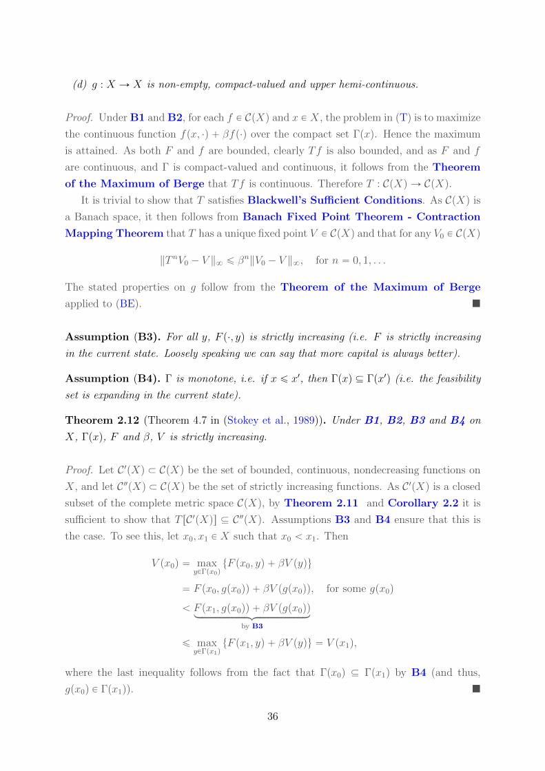
(d) g : X Ñ X is non-empty, compact-valued and upper hemi-continuous.

Proof. Under B1 and B2, for each f P CpXq and x P X, the problem in (T) is to maximize

the continuous function fpx, ¨q ` βfp¨q over the compact set Γpxq. Hence the maximum

is attained. As both F and f are bounded, clearly Tf is also bounded, and as F and f

are continuous, and Γ is compact-valued and continuous, it follows from the Theorem

of the Maximum of Berge that Tf is continuous. Therefore T : CpXq Ñ CpXq.It is trivial to show that T satisfies Blackwell’s Sufficient Conditions. As CpXq is

a Banach space, it then follows from Banach Fixed Point Theorem - Contraction

Mapping Theorem that T has a unique fixed point V P CpXq and that for any V0 P CpXq

‖T nV0 ´ V ‖8 ď βn‖V0 ´ V ‖8, for n “ 0, 1, . . .

The stated properties on g follow from the Theorem of the Maximum of Berge

applied to (BE). �

Assumption (B3). For all y, F p¨, yq is strictly increasing (i.e. F is strictly increasing

in the current state. Loosely speaking we can say that more capital is always better).

Assumption (B4). Γ is monotone, i.e. if x ď x1, then Γpxq Ď Γpx1q (i.e. the feasibility

set is expanding in the current state).

Theorem 2.12 (Theorem 4.7 in (Stokey et al., 1989)). Under B1, B2, B3 and B4 on

X, Γpxq, F and β, V is strictly increasing.

Proof. Let C 1pXq Ă CpXq be the set of bounded, continuous, nondecreasing functions on

X, and let C2pXq Ă CpXq be the set of strictly increasing functions. As C 1pXq is a closed

subset of the complete metric space CpXq, by Theorem 2.11 and Corollary 2.2 it is

sufficient to show that T rC 1pXqs Ď C2pXq. Assumptions B3 and B4 ensure that this is

the case. To see this, let x0, x1 P X such that x0 ă x1. Then

V px0q “ maxyPΓpx0q

tF px0, yq ` βV pyqu

“ F px0, gpx0qq ` βV pgpx0qq, for some gpx0q

ă F px1, gpx0qq ` βV pgpx0qqlooooooooooooooomooooooooooooooon

by B3

ď maxyPΓpx1q

tF px1, yq ` βV pyqu “ V px1q,

where the last inequality follows from the fact that Γpx0q Ď Γpx1q by B4 (and thus,

gpx0q P Γpx1q). �

36

Assumption (B5). F is strictly concave. For px, yq P A and px1, y1q P A such that

px, yq ‰ px1, y1q and for all λ P p0, 1q,

F pλpx, yq ` p1´ λqpx1, y1qq ą λF px, yq ` p1´ λqF px1, y1q.

Assumption (B6). Γ is convex, i.e. for all λ P p0, 1q and for all x, x1 P X and y P Γpxq

and y1 P Γpx1q,

λy ` p1´ λqy1 P Γpλx` p1´ λx1qq.

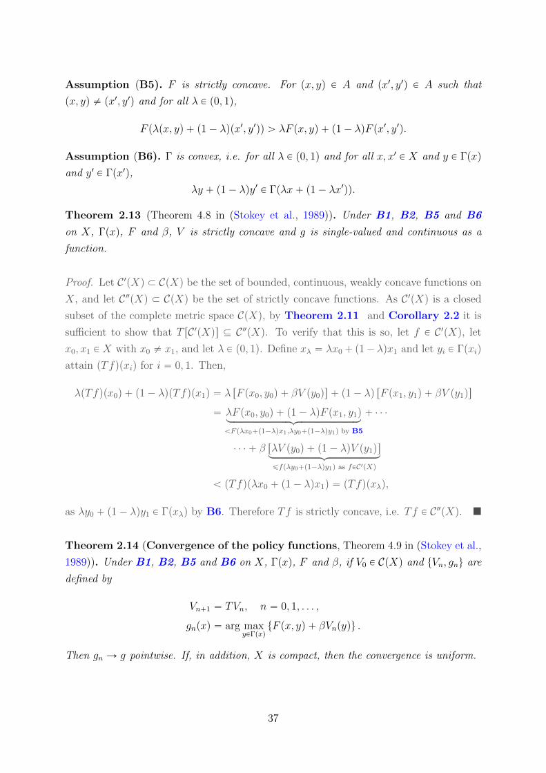
Theorem 2.13 (Theorem 4.8 in (Stokey et al., 1989)). Under B1, B2, B5 and B6

on X, Γpxq, F and β, V is strictly concave and g is single-valued and continuous as a

function.

Proof. Let C 1pXq Ă CpXq be the set of bounded, continuous, weakly concave functions on

X, and let C2pXq Ă CpXq be the set of strictly concave functions. As C 1pXq is a closed

subset of the complete metric space CpXq, by Theorem 2.11 and Corollary 2.2 it is

sufficient to show that T rC 1pXqs Ď C2pXq. To verify that this is so, let f P C 1pXq, let

x0, x1 P X with x0 ‰ x1, and let λ P p0, 1q. Define xλ “ λx0` p1´ λqx1 and let yi P Γpxiq

attain pTfqpxiq for i “ 0, 1. Then,

λpTfqpx0q ` p1´ λqpTfqpx1q “ λ rF px0, y0q ` βV py0qs ` p1´ λq rF px1, y1q ` βV py1qs

“ λF px0, y0q ` p1´ λqF px1, y1qloooooooooooooooooomoooooooooooooooooon

ăF pλx0`p1´λqx1,λy0`p1´λqy1q by B5

` ¨ ¨ ¨

¨ ¨ ¨ ` β rλV py0q ` p1´ λqV py1qsloooooooooooooomoooooooooooooon

ďfpλy0`p1´λqy1q as fPC1pXq

ă pTfqpλx0 ` p1´ λqx1q “ pTfqpxλq,

as λy0 ` p1´ λqy1 P Γpxλq by B6. Therefore Tf is strictly concave, i.e. Tf P C2pXq. �

Theorem 2.14 (Convergence of the policy functions, Theorem 4.9 in (Stokey et al.,

1989)). Under B1, B2, B5 and B6 on X, Γpxq, F and β, if V0 P CpXq and tVn, gnu are

defined by

Vn`1 “ TVn, n “ 0, 1, . . . ,

gnpxq “ arg maxyPΓpxq

tF px, yq ` βVnpyqu .

Then gn Ñ g pointwise. If, in addition, X is compact, then the convergence is uniform.

37

Proof. Let C2pXq Ă CpXq be the set of strictly concave functions f : X Ñ R. As

shown in Theorem 2.13, V P C2pXq. Besides, as shown in the proof of that theorem,

T rC 1pXqs Ď C2pXq. As V0 P C 1pXq, it then follows that every function Vn, n “ 1, 2, . . . is

strictly concave. Define the functions tfnu and f by

fnpx, yq “ F px, yq ` βVnpyq, n “ 1, 2, . . . ,

fpx, yq “ F px, yq ` βV pyq.

As F satisfies B5, it follows that each function fn, n “ 1, 2, . . . is strictly concave as f is.

Therefore Theorem 2.13 applies and the desired results are proved. �

Once we have shown that it exists a unique solution V P CpXq to the functional

equation (BE), we would like to treat the maximum problem in that equation as an

ordinary programming problem and use the standard methods of calculus to characterize

the policy function g. For example, consider the one-sector neo-classical growth model:

V pkq “ maxk1PΓpkq

tupfpkq ´ k1q ` βV pk1qu .

If we knew that V was differentiable (and the solution to (BE) was always interior), then

the policy function g would be given implicitly by the first-order condition

´ u1pfpkq ´ gpkqq ` βV 1pgpkqq “ 0.

Besides, if we knew that V was twice differentiable, the monotonicity of g could be

established by differentiating the previous expression with respect to k and examining

the resulting expression for g1. However, this ultimately depends upon the differentiable

of the functions u, f , V and g. We are free to make any differentiability assumptions on

u and f , but the properties of V and g must be established.

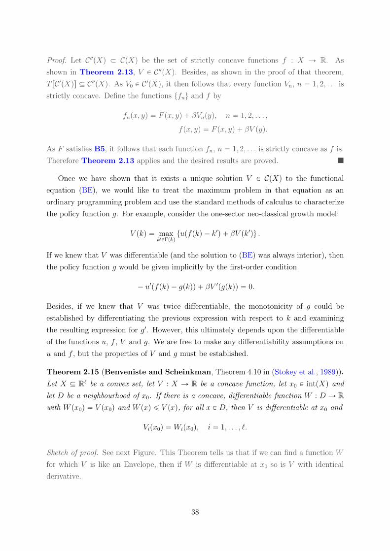
Theorem 2.15 (Benveniste and Scheinkman, Theorem 4.10 in (Stokey et al., 1989)).

Let X Ď R` be a convex set, let V : X Ñ R be a concave function, let x0 P intpXq and

let D be a neighbourhood of x0. If there is a concave, differentiable function W : D Ñ Rwith W px0q “ V px0q and W pxq ď V pxq, for all x P D, then V is differentiable at x0 and

Vipx0q “ Wipx0q, i “ 1, . . . , `.

Sketch of proof. See next Figure. This Theorem tells us that if we can find a function W

for which V is like an Envelope, then if W is differentiable at x0 so is V with identical

derivative.

38

xx0

V pxq

W pxq

See Stokey et al. (1989, p.85) for a complete proof. �

Assumption (B7). F is continuously differentiable in the interior of A.

Theorem 2.16 (Differentiability of the value function, Theorem 4.11 in (Stokey

et al., 1989)). Under Assumptions B1, B2, B5, B6 and B7 on X, Γpxq, F and β,

if x0 P intpXq and gpx0q P intrΓpx0qs, then V is continuously differentiable at x0 with

derivatives given by

Vipx0q “ Fipx0, gpx0qq, i “ 1, . . . , `.

Proof. The proof relies on Theorem 2.15. As gpx0q P intrΓpx0qs and γ is continuous, it

follows that gpx0q P intrΓpxqs for all x is some neighbourhood D of x0. Define W on D by

W pxq “ F px, gpx0qq ` βV pgpx0qq.

As F is concave by B5 and differentiable by by B7, it follows that W is concave and

differentiable. Moreover, as gpx0q P intrΓpxqs for all x P D, it follows that

W pxq ď maxyPΓpxq

tF px, yq ` βV pyqu “ V pxq, for allx P D,

with equality at x0. Then V and W satisfy the hypothesis of Theorem 2.15, and thus

V is differentiable at x0 with

Vipx0q “ Fipx0, gpx0qq, i “ 1, . . . , `.

�

39

References

Guner, N. (2008), Advanced Macroeconomic Theory, Lecture Notes.

Juan Pablo Rincon-Zapatero (n.d.), Mathematics, Lecture Notes.

Rincon-Zapatero, J. P. and Santos, M. S. (2009), Differentiability of the value function

without interiority assumptions, Vol. 144.

Stokey, N. L., Lucas, R. E. and Prescott, E. (1989), Recursive Methods in Economic

Dynamics, Harvard University Press.

40

A Appendix: Envelope Theorem

Let Xt “ R, and consider the Bellman equation

VtpXtq “ supXt`1PΓtpXtq

tFtpXt, Xt`1q ` βVt`1pXt`1qu , t “ 0, 1, . . . (33)

with associated policy function (correspondence)

gtpXtq “ arg supXt`1PΓtpXtq

tFtpXt, Xt`1q ` βVt`1pXt`1qu , t “ 0, 1, . . . (34)

Proposition A.1 ((Weak) Envelope Theorem). Let Vt`1pXt`1q : RÑ R and FtpXt, Xt`1q :

RˆRÑ R be differentiable. Then if the optimal policy function (or correspondence) sat-

isfies

• gtpXtq is a differentiable function, and

• gtpXtq P int pΓtpXtqq

then Vtpxtq : RÑ R is differentiable and

dVtpXtq

dXt

“BFtpXt, Xt`1q

BXt

ˇ

ˇ

ˇ

ˇXt“X˚

Xt`1“gtpX˚q

Proof. Let us assume that everything is differentiable in (33). Then the F.O.C. w.r.t. the

choice variable Xt`1 assuming an interior solution at some Xt “ Xt is given by

dVtpXtq

dXt`1

ˇ

ˇ

ˇ

ˇ

Xt“Xt

“ 0 ôBFtpXt, Xt`1q

BXt`1

ˇ

ˇ

ˇ

ˇ

Xt“XtXt`1“Xt`1

`dVt`1pXt`1q

dXt`1

ˇ

ˇ

ˇ

ˇ

Xt`1“Xt`1

“ 0 (35)

Let us evaluate the Bellman equation (33) at the optimum given by (34), obtaining

VtpXtq “ FtpXt, gtpXtqq ` βVt`1pgtpXtqq.

At any arbitrary point Xt “ Xt, the derivative of this expression w.r.t the state variable

Xt is given by

dVtpXtq

dXt

ˇ

ˇ

ˇ

ˇ

Xt“Xt

“BFtpXt, gtpXtqq

BXt

ˇ

ˇ

ˇ

ˇXt“Xt

Xt`1“gtpXtq

`BFtpXt, gtpXtqq

BgtpXtq

ˇ

ˇ

ˇ

ˇXt“Xt

Xt`1“gtpXtq

¨dgtpXtq

dXt

`

`dVt`1pgtpXtq

dgtpXtq

ˇ

ˇ

ˇ

ˇXt“Xt

Xt`1“gtpXtq

¨dgtpXtq

dXt

“

»

–

BFtpXt, gtpXtqq

BgtpXtq

ˇ

ˇ

ˇ

ˇXt“Xt

Xt`1“gtpXtq

`dVt`1pgtpXtq

dgtpXtq

ˇ

ˇ

ˇ

ˇXt“Xt

Xt`1“gtpXtq

fi

fl

dgtpXtq

dXt

`

`BFtpXt, gpXtqq

BXt

ˇ

ˇ

ˇ

ˇXt“Xt

Xt`1“gtpXtq

“BFtpXt, gpXtqq

BXt

ˇ

ˇ

ˇ

ˇXt“Xt

Xt`1“gtpXtq

41

where the last equality uses (35). Since Xt was arbitrarily chosen, it also holds for

Xt “ X˚, so thatdVtpXtq

dXt

“BFtpXt, Xt`1q

BXt

ˇ

ˇ

ˇ

ˇXt“X˚

Xt`1“gtpX˚q

�

42