Dynamic Modelling of Battery Cooling Systems for...

Dynamic Modelling of Battery Cooling Systems

for Automotive Applications

Master’s Thesis within the International Master’s Program: Sustainable Energy Systems

FABIAN HASSELBY

Department of Energy and Environment

Division of Heat and Power Technology

CHALMERS UNIVERSITY OF TECHNOLOGY

Göteborg, Sweden 2013

I

MASTER’S THESIS

Dynamic Modelling of Battery Cooling Systems for

Automotive Applications

Master’s Thesis within the International Master’s Program: Sustainable Energy Systems

FABIAN HASSELBY

SUPERVISORS:

Sam Gullman (Volvo Car Corporation)

Thomas Landelius (Volvo Car Corporation)

Mathias Gourdon (Chalmers University of Technology)

EXAMINER

Mathias Gourdon



CHALMERS UNIVERSITY OF TECHNOLOGY


II

Dynamic Modelling of Battery Cooling Systems for Automotive Applications

Master’s thesis within the International master’s Program: Sustainable Energy Systems

FABIAN HASSELBY

© FABIAN HASSELBY, 2013



Chalmers University of Technology

SE-412 96 Göteborg

Sweden

Telephone: + 46 (0)31-772 1000

Chalmers Reproservice


I

Dynamic Modelling of Battery Cooling Systems for Automotive Applications

Master’s thesis within the International master’s Program: Sustainable Energy Systems

FABIAN HASSELBY Department of Energy and Environment


Chalmers University of Technology

ABSTRACT

The automotive industry is currently undergoing a period of historic upheaval. Under

mounting pressure from increasing fuel costs and emission legislations, the industry

now faces numerous challenges wherein the reduction of consumed energy and

emission mitigation become principal. In light of these circumstances the hybrid

electric vehicle technology is emerging. With its aptitude for combining the benefits

of both the internal combustion engine and those of the electrical vehicle, the hybrid

electrical vehicle is presently becoming more of a viable option.

Any further improvement done to enhance the range and performance of the vehicle

does, however, come at a cost. Frequent charge- and discharge cycles lead to residual

heat build-up within the cells and will, if left unchecked, causes increased cell

degradation, which in turn decreases the lifetime of the cells as well as battery

performance. Consequently, finding methods for cooling these cells to their preferred

temperature range becomes essential.

In this thesis work a One Dimensional Computational Fluid Dynamics (1D CFD)

modelling approach was taken in order to construct and evaluate a model of a hybrid

electric vehicle’s battery thermal management system. The study showed that it is

possible to build a complete model of such a system capable of producing accurate

predictions with only slight deviations from actual measurements. The benefits of

using such models early on in the vehicle development stages was also exemplified by

using the model to conceive a possible control scheme for cooling the battery in an

energy efficient manner. The findings from this study revealed that designing an

energy efficient method of controlling the system is a difficult endeavour, not only

because of the many constraints placed on an actual system, as well as, it’s dynamic

behaviour, but also due to the way one chooses to measure efficiency improvements.

It is likely that a more comprehensive analysis would yield other and better control

strategies than the example demonstrated in this thesis work.

Key words: 1D CFD, CFD, CAE, Modelling, Simulation, Battery Cooling, Battery

Thermal Management, GT-SUITE

II

Dynamisk modellering av batterikylsystem för fordonsapplikationer

Examensarbete inom masterprogrammet Sustainable Energy Systems

FABIAN HASSELBY

Institutionen för energi och miljö

Avdelningen för värmeteknik och maskinlära

Chalmers tekniska högskola

SAMMANFATTNING

Fordonsindustrin genomgår för närvarande en historisk förändring. Branschen står

idag inför många nya utmaningar som följd av stigande bränslekostnader och hårdare

emissionskrav vilket medför att faktorer som minskad energianvändning och

utsläppsreduktion blir helt avgörande. Med dessa omständigheter som bakgrund

börjar andra tekniker träda fram. Med sin fallenhet för att kombinera nyttorna hos

både förbränningsmotorn och den elektriska motorn börjar nu elhybridfordon bli ett

allt mer fördelaktigt alternativ.

Att ytterligare förbättra räckvidden och prestandan hos elhybriderna är en

komplicerad fråga. Frekventa laddnings- och urladdningscykler leder till att restvärme

byggs upp i cellerna vilket kan orsaka oönskad nedbrytning, som i sin tur påverkar

livslängden hos cellerna samt batteriets prestanda. Det är därmed helt avgörande att

lyckas med att utveckla metoder för att kyla cellerna till ett lämpligt

temperaturområde.

I detta examensarbete användes en endimensionell flödesmodelleringsmetod, Eng:

One Dimensional Computational Fluid Dynamics (1D CFD), för att konstruera och

utvärdera en modell av ett batterikylsystem till en elhybrid. Studien visade att det är

möjligt att skapa en komplett systemmodell av ett sådant system som i sin tur klarar

av att ta fram korrekta resultat med endast små avvikelser från faktiska mätningar. För

att visa fördelarna med att använda liknande modeller i tidigt skede inom

fordonsutveckling användes modellen även till att skapa ett enkelt reglersystem för

kylning av batteriet på ett energieffektivt sätt. Resultaten från studien visade att

utformningen av ett energieffektivt reglersystem är en komplicerad frågeställning, inte

enbart på grund av de många krav som ställs på ett verkligt system samt dess

dynamiska beteende, men även som följd av det sätt man väljer mäta förbättring i

energieffektivt. Det är troligt att en mer omfattande analys skulle ge andra och bättre

metoder för att reglera ett kylsystem än dem som togs fram i detta arbete.

Nyckelord: 1D CFD, CFD, CAE, Modellering, Simulation, Batterikylning, GT-

SUITE

III

Contents

ABSTRACT I

SAMMANFATTNING II

CONTENTS III

PREFACE V

NOTATIONS VI

1 INTRODUCTION 1

1.1 Background 1

1.2 Objective 4

1.3 Methodology 4

1.4 Assumptions and Delimitations 5

2 THEORY 7

2.1 Computational Fluid Dynamics 7

2.2 Heat Transfer 8 2.2.1 Forced Flow Single-Phase Heat Transfer 10

2.2.2 Forced Flow Two-Phase Vaporising Heat Transfer 11

2.3 Pressure Drop 11

2.3.1 Two-Phase Pressure Drop 12

3 COMPONENT MODELLING 13

3.1 The Chiller Component 13 3.1.1 Chiller Geometry and Flow Scheme 13 3.1.2 Chiller Data-Set 15 3.1.3 Chiller Modelling 16

3.2 Heat Transfer Calibration and Simulation 17 3.2.1 Heat Transfer Results 19

3.3 Pressure Drop Calibration and Simulation 20 3.3.1 Coolant-Side Pressure Drop Results 22 3.3.2 Refrigerant Pressure Drop Results 24

3.4 The External Heat Exchanger 26 3.4.1 External Heat Exchanger Modelling 27

3.4.2 External Heat Exchanger Model Results 28

3.5 The Internal Battery Cooling System 30 3.5.1 Internal Battery Cooling System Modelling 31 3.5.2 Internal Battery Cooling Model Results 34

3.6 The Radial Pump 37

4 CIRCUIT MODELLING 39

IV

5 CONTROL STRATEGY 41

5.1 Control Strategy Results 43

5.2 Discussion 49

6 CONCLUSIONS 51

6.1 Conclusions 51 6.1.1 Future Work 52

7 BIBLIOGRAPHY 53

APPENDIX A 55

APPENDIX B 59

APPENDIX C 61

V

Preface

To begin with, I would like to thank my supervisor at Volvo Car Corporation, Sam

Gullman, for his insightful advice, constant guidance, and for his tireless effort in

educating me in his profession. Not only has he and his closest colleges supplied me a

continuous stream of knowledge, they have also inspired and shown me what working

as an engineer may entail.

Additionally I would like to extend my gratitude to Mathias Gourdon, my supervisor

at Chalmers University of Technological, and to all the employees at VCC who have,

directly or indirectly, been involved in my work. Without your support this work

would never have come as far as it did.

This research was conducted at VCC, Gothenburg, between January and June 2013.

The work was carried out at the department of Climate System Development, and was

done in collaboration between different departments, such as, the departments of

Electrical Propulsion Systems and of Cooling Systems.

Gothenburg, Sweden, 2013

VI

Notations

D1 One Dimensional

D3 Three Dimensional

CAE Computer Aided Engineering

CFD Computational Fluid Dynamics

HX Heat Exchanger

DOE Design of Experiments

COP Coefficient of Performance

Opt Optimum Strategy

Ref Reference Strategy

.condQ

Thermal conduction heat transfer rate [W]

.convQ

Thermal convection heat transfer rate [W]

radQ

Thermal radiation heat transfer rate [W]

isimQ

,

Simulated Heat Transfer [W]

idataQ

,

Measured Heat Transfer [W]

k Thermal conductivity [W m-1

K-1

)] A Area [m

2]

x Spatial direction [-]

h Heat transfer coefficient [W m-2

K-1

)] Emissivity [-] Stefan-Boltzmann constant [W m

-2 K

-4]

v Viscosity [Pa s] Density [kg m

-3]

c Velocity [m s-1

]

f Darcy friction factor [-]

L Length [m] d Diameter [m] g The gravity of Earth [m s

2]

fh Total head loss [m]

2 Two-phase multiplier [-]

P Power [W]

T Temperature [°C]

p Pressure [bar]

pC Heat capacity [J g-1

K-1

]

hD Hydraulic diameter [m]

Objf Objective function

Pr Prandtl number Nu Nusselt number Re Reynolds number

Co Convection number Fr Froude number Bo Boiling number

We Weber number

1

1 Introduction

1.1 Background

Vehicle development has traditionally had a heavy focus on fuel economy,

specifically the powertrain development and optimizing the engine and drivetrain. To

optimize all energy consumers is a more difficult task, since they are more dispersed

and interdependent. With hybrid vehicles rolling in and engines getting better and

better there is a need to focus in new areas or advanced technologies to further bring

down fuel-consumption. To manage this task new methods are required, specifically

1D-CFD flow type system modelling and heat exchange. This way a model can

integrate all energy consumers and attempt balancing and optimizing tasks earlier and

more efficiently in the development process. For hybrid vehicles the thermal

management of the battery is such a system, where there is a need for a fully transient

model of the system.

Thermal management of battery systems are essential to ensure satisfactory vehicle

operation. Frequently charging and discharging a vehicle’s battery inevitably leads to

heat generation throughout battery cells, and without a well thought out cooling

system managing this thermal behaviour, the battery may risk severe consequences.

For vehicle applications today, higher energy density of a battery is often advocated to

increase range of the electrical driveline in hybrids vehicles. A technology with these

features is the Lithium-ion battery. The use of this battery type has increased over the

years and is today usually preferred over other battery technologies due to the

potentially higher energy density, ~400Wh/litre. The battery technology is applicable

to a wide range of portable devises, and is now replacing nickel-metal hydride

batteries, NiMH-batteries, found in products such as touchpads, smart phones, laptops

and power tools. The potential of having high energy or power density has made Li-

ion batteries an attractive choice for the hybrid vehicle niche market, allowing

vehicles to provide longer driving ranges and improved acceleration. The ever

increasing customer demand does, however, pose new challenges. Faster charge

cycles, higher acceleration, increased energy/power demand, the already limited

vehicle space, and the overall complexity of a modern vehicle today, demand that the

battery and its thermal management system are constructed and maintained with the

highest of standards. Therefore the principal obstacles to overcome when improving

battery performance have been safety, performance, and battery duration. These

factors are all very dependent on temperature.

Though low cell temperature lead to decreased battery performance, preventing high

temperature throughout a battery has become a chief concern for automotive

applications. High temperatures lead to increased chemical reaction rates in the cells,

causing increased degradation of the cells and decreasing the longevity of the battery.

Furthermore, increased temperatures lead to lowering of the charge- and discharge

efficiency. For a Li-ion cell the lifespan of the cell is reduced by approximately two

months for every degree of temperature rise in an operating range between 30 to 40

°C (Salvio C, Youngmann M, 2000). To attain a full lifespan, a cell’s temperature

should therefore be kept below 40 °C. The temperature gradient, between the cell and

it surroundings, should be kept below 5 °C in order to avoid non-uniform

temperatures within the battery. Non-uniformity adversely affects the lifetime and

performance of the cells (Salvio C, Youngmann M, 2000). Increased temperatures

2

also relate to safety issue concerns if the cells are not thermally managed. Sharp heat

generation, during tasking conditions such as large power usage, may lead to

overheating in the cells and result in thermal runaway propagation in the battery.

Overheating is also known to be caused by defective cells. The best operational range

for Li-ion cells spans a quite small temperature range and lies between 20 to 40 °C

(Yeow K, et al., 2012).

Thermal generation in battery cells can be decomposed into three fundamentals:

Reaction heat, Joule heat, and polarisation heat. These factors contribute to the cells

overall heating to different degrees and may be expressed as functions of the charge

and discharge processes. Reaction heat is generated a result of the chemical reactions

in the cells and corresponds to the thermal energy of the reactions. Joule heating is

done through the components conveying electricity in the battery, and is caused by the

electrical resistance. Polarisation heat is a term associated with the electro-chemical

polarisation of the battery where energy loss occurs due to polarisation. The

polarisation heat term expresses heat generation during charge and discharge (Sato,

2000).

Addressing the matter of how much cooling is required becomes more intuitive when

comparing the heat generation in different cells during various conditions. Below, in

table 1.1, the thermal generation is given for two typical battery modules; the nickel-

metal hydride and the Lithium-ion.

Table 1.1. Heat generation from typical HEV/EV modules (Pesaran A.A, 2001)

Heat Generation [W/Cell]

Battery Type Cycle 0°C 22-25°C 40-50°C

NiMH, 20Ah C/1 Discharge, 70% to 35 % State

of Charge

- 1.19 1.11

NiMH, 20Ah 5C Discharge, 70% to 35 % State of

Charge

- 22.79 25.27

Li-Ion, 6Ah C/1 Discharge, 80% to 50 % State

of Charge

0.6 0.04 -0.18

Li-Ion, 6Ah 5C Discharge, 80% to 50 % State of

Charge

12.07 3.50 1.22

Table 1.1, indicates that the cells generate more heat as the discharge rate increases,

and that in general more heat is generated as the temperature decreases because of an

increase in resistance within the cells. The negative sign, shown for the Li-ion cell

during 5C discharge at 40-50°C, reveals that the electro-chemical reactions in the cells

could become endothermic as opposed to exothermic (Pesaran A.A, 2001). To relate

the generation of each cell to an entire battery it is reasonable to consider a battery

having 200 cells. In this scenario the total heat generation then becomes 700 W, for a

battery with Li-ion cells during 5C discharge and a cell temperature between 22-25 °C.

A general battery pack for vehicle application is, as mentioned, composed of a large

number of cells to provide the required power. The compactness of battery packs

poses a challenge for effective thermal management. Various battery thermal

management systems have been developed for air- and liquid cooling as well as

passive cooling to prevent overheating and thermal runaway propagation without

3

over-dimensioning the cooling system. The most effective systems require some form

of active cooling using a liquid coolant, which requires energy input. The challenge

lies in constructing a system where sufficient cooling is ensured without drawing too

much power. Because of the hybrid vehicle being an isolated system, power is not

readily obtainable and any power usage in the system therefore leads to decreased

vehicle range and reduced energy availability for other energy consuming utilities.

The scarcity of available energy is one additional reason for why finding optimised

ways of controlling thermal management system is of great importance.

In this thesis project, a thermal management system in a hybrid vehicle has been

investigated. The studied cooling system is depicted in the schematic overview below,

figure 1.1. To be more precise, the schematic provides a holistic view of both the

hybrid vehicle’s battery thermal management system and its AC-system, which is

directly connected to the battery cooling system through a plate heat-exchanger.

Figure 1.1. Overview of both the battery cooling system and connecting AC-system

The battery’s active cooling system may be decomposed into the following main

components: a Chiller plate heat exchanger, an internal battery cooling system, a

radial pump, and an external heat exchanger. As mentioned, the AC-system is

connected through the Chiller component and the system is principally operating

using a vapour-compression refrigeration cycle.

The Chiller is tasked with transferring heat between the battery cooling system’s

liquid, referred to as the coolant, and the AC-systems fluid, referred to as the

refrigerant. Both systems operate using different working mediums. In the cooling

system the medium used is an Ethylene Glycol based water solution, having a mixture

with the following proportions: 50 % Ethylene Glycol with 50 % distilled water. In

the AC-system the refrigerant R134a is used as circulation fluid and is a commonly

used refrigerant for refrigeration cycles. Elaborating further on the Chiller, this

component facilitates heat transfer between the two systems, with the intention of

cooling the coolant stream. During this operation the refrigerant entering the Chiller

on the AC-side is being evaporated.

4

Since the system uses an active cooling method power is required by the following

three components: system pump, external HX fan, and indirectly by the AC-system’s

compressor via the Chiller.

1.2 Objective

The main objective of this thesis work was to perform all necessary steps to develop

an accurate, transient model of a battery thermal management system. The model is of

a specific part included in a hybrid car project at Volvo Car Corporation, VCC, and

was used to solve a balancing task focused on reducing the energy demand in this

project. The products of the work are threefold: 1:st) The model itself, which will be

able to be integrated with other models of energy consumers and used in the

development-work, 2:nd) The optimization task chosen where the conclusions will be

implemented in the control system for the car, and 3:ed) Actual method and process

used to develop the model which will be used to develop similar models in the future.

The objectives of this study are summarised in the list below:

Data retrieval – Collect reliable information and performance data regarding

the system, and its components.

Modelling and Calibration – Construct models of the systems components and

integrate them to form the larger circuit. Calibrate the models to correlate with

the empirical data if modelling is not sufficient.

Model validation – Validate the model to ascertain its accuracy.

Control strategy – Conduct a study on the systems control method to find

energy efficient methods of cooling the battery’s cells, and to promote the use

of 1D-CFD models.

1.3 Methodology

To complete the tasks set forth, a 1D-CFD modelling tool was used to construct and

test a model of the hybrid vehicles battery cooling system. The proposed software was

the GT-Suite modelling tool, a commercial program developed for use in vehicle

development.

The battery circuit itself is a system incorporating numerous components. Most of

these components were required in the complete model, while others were discarded

to limit the complexity of the model. Components chosen for exclusion were for

instance; valves and electrical components. The overall approach for modelling the

entire circuit was to initially model all its separate components and then combine

these to form the larger cooling system.

Alongside the work of modelling the circuit, collecting reliable test data and

component properties became essential. The test data was used during the modelling

process to correlate the component models to the measurement data. This is a crucial

step since the model needs to behave in a manner that later can be explained and

relied upon.

After the model was fully calibrated further examination was needed to ascertain the

model’s validity and reliability. The validation part of the project entailed running

additional simulations with the component models and comparing the results with

different empirical data.

5

1.4 Assumptions and Delimitations

An overlying assumption made in this study can be attributed to the overall circuit, in

which it was assumed that having obtained reliable systems components would be

sufficient to ensure high system accuracy. Without empirical results from the entire

system it was impossible to verify this assumption and it should be stated that every

effort has been taken to ensure the accuracy of the numerical factors of this study.

Although the empirical data used for validation and calibration of model components

was regarded to be of good quality, some limitations were identified. Concerning the

Chiller component’s in-data, the information used was based on the suppliers own

model of the component and not on actual test results. This meant that the accuracy of

the in-data depended on the reliability of the supplier’s model, which according to the

supplier was sufficient. The reasoning concerning the reliability of data can be

extended to actual empirical results as well, and depends on how the tests were

conducted.

Additional limitations concern the internal battery cooling model. In this model in-

data information had been collected using a battery concept already available for

consumers. In these tests only measurements on inlet- and outlet temperatures and

mass flow were done, and no information regarding internal temperatures, flow, and

electrical behaviour of active cells was found. Verifying the behaviour of the internal

battery cooling was therefore only done to its extremities, although it was reason that

simulation results collected from within the model were accurate. Another intentional

shortcoming of the model is that it is not adapted to determine electro-chemical

behaviour within the cells. The model instead focused on predicting thermal and fluid

behaviour within the internal system and was able to do this accurately.

Regarding the validation which was done on the Internal Battery System, the

comparative information had been collected during testing under specific conditions.

Strictly speaking this implies that the model has only verified for a certain ambient

temperature and during conditions were the battery cells were not used. Regardless of

the narrow range of validation, the model accurately predicts the in- and outgoing

temperatures to the component and thereby the heat transfer done across internal

system. This is also true for a system where active heat generating cells are used due

to that the heat transfer characteristics of the system were identified. Another

difference between the model and measurements was that the system had been created

to be closed off to ambient conditions as opposed to the measurement which used an

un-insulated battery. The effects of this were corrected for using the calibration values

making the model act as un-insulated.

Further drawbacks to system accuracy were done when retrieving data for the pump

and fan model. Here no readily obtainable data was found and instead a MATLAB

script was created to extract information from charts. This program script used a

visual method of obtaining data by means of manually collecting the information from

the charts and the errors that occurred were estimated to be small.

Concerning the calibration method adopted for large sections of this work, it should

be stated that the calibration was decided to be accurate once the simulation results

correlated with the measurements of a component. Investigating the properties of the

individual calibration parameters was only done to consider how reasonable they

became since the goal of the method was to ensure that the model predicted accurate

values for the correlated quantity.

7

2 Theory

2.1 Computational Fluid Dynamics

Computational Fluid Dynamics or CFD is a numerical method used for analysing the

behaviour of systems involving fluid flow, heat transfer, and related phenomena such

as combustion, diffusion, and chemical reactions. The method is powerful and

practised to great extent by many industries and in research.

The most commonly used form of CFD code is based on the finite volume technique,

in which the domain volume is discretised, i.e. divided, into smaller discrete volumes.

These smaller volumes, often referred to as cells, are then used in the computational

method where the governing equations are applied to the contents of these volumes.

The governing partial differential equations solved for are the Navier-Stokes

equations on fluid flow. The equations represent the following conservation laws of

physics; conservation of, mass, momentum (Newton’s second law of motion) and

energy (the first law of thermodynamics). To exemplify what this entails for the

contents of a single volume, the conservation of a flow variable such as velocity may

be formulated as an equation balancing the level of increase or level of decrease. In

words: The rate of change of a variable with respect to time is equal to the net flux of

transported into the volume, done by convection and diffusion, plus the net rate of

creation of the variable inside the volume. (Versteeg H.K, Malalasekera W, 1995)

In this work the commercial 1D CFD analysis code GT-SUITE was used. The

program environment is developed by Gamma Technologies Inc. and incorporates a

1D computational approach to solve the fluid dynamic equations governing the

system. The 1D CFD method solves the partial differential Navier-Stokes equations in

one dimension, which means averaging quantities across the flow direction (Gamma

Technologies Inc, 2012). As opposed to full 3D CFD, where the equations are solved

for all directions.

Determining the flow in a model is done by solving the 1D compressible flow

equations, which are linearised for the conservation equations. Further, the system is

discretised into smaller volumes as in the 3D CFD case, although in the 1D version

the quantities become averaged. The governing equations are applied to the system

and the solver then calculates the scalar quantities of the conservation equations for

mass and energy in each volume, and the momentum equations for each boundary

between the volumes. The solver, i.e. the CFD code, uses the finite difference

technique combined with a finite volume approach to discretise and numerically

calculate the governing equations. An illustrative example of the 1D method is show

in figure 2.1.

8

Figure 2.1. An example on a simple 1D flow domain, where scalar quantities, such as temperature,

pressure and enthalpy, are solved for in the cells and vector quantities, such as velocity and mass flux,

are solved for at the boundaries.

The models in GT-SUITE are created by using various building blocks corresponding

to a systems different parts and vary in their degree of complexity; from simple pipes

objects to more refined objcets such as heat-exchangers and engine blocks. The blocks

are then joined together through junctions. A 1D CFD model comprises of an entire

network of blocks and junctions where each block is given a predetermined set of

parameters which defines their physical behaviour. Using these buidling blocks, more

elaborat components or systems can be constructed such as a model of an entire AC-

system.

Due to the objective of this study was to construct a transient model model of a hybrid

vehicle’s battery thermal management system, properties such as heat transfer and

pressure drop were of primary concern. Both these quanteties are determined by

solving the governing equations as well as by using correlations when requierd. The

solution may be refined by including, or changing to, more physial and/or emperical

correlations. For heat transfer this may for example involve changing a correlation to

one that better describes the physical behaviour. In the upcoming chapter the theory

and underlying reasoning used throughout this thesis work is presented for heat

transfer and pressure drop.

2.2 Heat Transfer

“Heat transfer is the science of the rules governing the transfer of heat between

systems of different temperatures” (Böckh P, Wetzel T, 2011). Heat transfer occurs

through the following three different modes; conduction, convection and radiation.

The modes do not necessarily all have to coincide at the same time, and may occur

separately depending on the system at hand. Consider a stationary system with a

single solid body, and where on either side of this body two different temperatures are

present. In such a system the dominating mode of heat transfer is conduction. If

instead the solid body resided in a system where a fluid was allowed to flow adjacent

to one side of the body, the heat transport to the fluid would then be governed by

convection. In reality thermal radiation is also present and occurs between two

surfaces having different temperatures through the transport of electromagnetic

waves.

Conduction occurs when a spatial temperature gradient is present in materials, and for

static materials only depends on material properties and the temperature gradient. The

temperature gradient facilitates the transfer of internal energy by diffusion and

9

collisions on the microscopic scale between molecules, atoms and electrons.

Conduction takes place for all states of matter, i.e. solid, liquid, gaseous, and with the

absence of external forces acting on the system, the differences in temperature decline

over time and eventually move toward thermal equilibrium (Böckh P, Wetzel T, 2011).

The conventional way of describing heat transfer through conduction is shown in

equation 1, below:

dx

dTAkQ

cond

. (1)

In equation 1, the term on the left hand side is the rate of heat transfer. The first term

on the right hand side, k, is the thermal conductivity which is both material and

temperature dependent. The area, A, is the cross sectional area of the object under

consideration. The last term on the left hand side is the temperature gradient in the

spatial direction orthogonal to the cross sectional area.

Convective heat transfer, or more commonly convection, is the combined effect of

thermal conduction and fluid motion. Between a solid wall and a fluid in motion, the

heat transfer is determined by thermal conductivity and by flow and material

parameters. When conditions allow for free convection the flow is caused by

gravitational forces due to differences in density as a result of a spatial temperature

gradient. If the flow on the other hand is caused by an external pressure differences

the heat transfer is said to be forced convection. Thermal convection is commonly

described as stated in equation 2.

)(.

TTAhQ sconv (2)

In equation 2, the convective heat transfer rate is determined by the product of the

heat transfer coefficient, h, surface area, As, and the temperature difference between

the surface temperature and the temperature of the fluid sufficiently far away from the

wall.

Thermal radiation occurs when electromagnetic waves are exchanged between

surfaces having different temperature. All gases and surfaces having three or more

atoms per molecule and a temperature above absolute zero emit waves of

electromagnetic energy.

)( 44

TTAQ srad (3)

In equation 3, the rate of heat transfer becomes a function of the emissivity of the

surface, ε, the Stefan-Boltzmann constant, σ, the radiating surface area, As, and the

difference in temperature to the power of four.

For cooling systems purposes, where the temperatures often are moderate, heat

transfer by thermal radiation is low and the dominant mods of heat transfer are

therefore conduction and convection.

10

2.2.1 Forced Flow Single-Phase Heat Transfer

Forced flow heat transfer through tubes is a common situation encountered in many

practical applications. For cooling systems this occurs in heat exchangers,

evaporators, condensers, pipes, ducts, and a multitude of other equipment. It is

therefore necessary to accurately estimate heat transfer coefficients in such situations.

The heat transfer coefficient between a fluid and a tube wall depends on a multitude

of different factors, such as tube wall material, dimensions, fluid properties, flow

movement, i.e. laminar- or turbulent flow, temperature differences between the wall

and fluid, and so on. The process of calculating the heat transfer coefficient is based

on experimental findings which are used to formulate correlations on the heat transfer

behaviour. These correlations are in turn formed using groups of dimensionless

variables in order to incorporate the factors mentioned above.

k

Cv p

Pr (4)

k

DhNu h

(5) v

Dc hRe (6)

The prandtl number, equation 4, is the ratio between the viscous diffusion rate and the

thermal diffusion rate. Equation 5, is the Nusselt number which is the ratio between

the convective heat transfer and the conductive heat transfer. The Reynolds number,

equation 6, is defined as the ratio of internal forces to viscous forces.

From the Nusselt expression the heat transfer coefficient can be obtained as shown in

equation 7. If necessary, it is possible to match the heat transfer behaviour of a given

pipe to measurements by scaling the heat transfer coefficient. This can be done by

introducing a heat transfer multiplier to heat transfer rate and thereby increase or

decrease the heat transfer rate in the pipe (Gamma Technologies Inc, 2012).

h

h

D

kNuh

k

DhNu

(7)

Many early studies has focused on investigating the single-phase heat transfer of

fluids in tubes in order to create correlations to model the heat transfer in other

geometries. A well-known empirical correlation for forced convection in water

through smooth tubes is the Dittus-Boeter equation given in equation 8 (Annaratone,

D, 2010). The correlation determines the Nusselt number, Nu, for forced flow in pipes

as a function of the Reynolds number, Re, and the Prandtl number, Pr, together with

an experimentally obtained coefficient and exponents. For the purposes of cooling

system investigated in this thesis, the coefficient in equation 8 was denoted as the

Coolant Turbulent Coefficient and the exponent above the Reynolds number as the

Coolant Turbulent Exponent. The use of these parameters will become clear later on

in the calibration sections of this study.

4.08.0 PrRe023.0 Nu (8)

Today numerous empirical correlations are available that treat the subject of heat

transfer in forces flow for tubes, ducts, heat exchangers, etc. Due to the nature of heat

transfer in forced flow convection, no universal function is currently available which

is able to describe the heat transfer for all possible situations.

11

2.2.2 Forced Flow Two-Phase Vaporising Heat Transfer

Heat transfer through vapour formation occurs by either the combination of the

nucleate boiling and convective vaporisation or by each mechanism separately. For

pure liquids flowing adjacent hot walls, nucleate boiling can take place before the

entire liquid reaches the boiling point temperature (Division of Heat & Power

Technology, Chalmers, 2012). The fluid entering the tube can either be saturated, sub-

cooled, or a mixture of both steam and liquid, and at the exit be wet, saturated or

superheated steam.

With increasing liquid temperature, and depending on fluid velocity, two-phase flow

convective heat transfer may develop. Convective boiling occurs when the heat transfer

coefficient of forced convection is greater than the heat transfer coefficient of the

nucleate boiling. With high fluid velocity the heat transfer coefficient becomes large

enough so that the surplus in temperature is not able to form nucleate sites at the walls

and the evaporation occurs on the surface of the liquid (Böckh P, Wetzel T, 2011).

Numerous methods and correlations exist for calculating heat transfer in developed

two-phase flow and are based on large bodies of experimental material. The

correlations are therefore dependent on the fluid used and only valid for certain

conditions. In this study the only medium being evaporated is the refrigerant

R134a, a widely used refrigerant, and to model the heat transfer occurring in this

process a correlation developed by Shah was implemented in the model (Fang X,

Shi R, Zhou Z, 2011).

Pr)Re,,,,( FrBoCofh phasetwo (9)

The correlation proposed by Shah for flow boiling heat transfer of the refrigerant

R134a is given in equation 9, as a function of the following dimensionless numbers;

the convection number, Co, the boiling number, Bo, the Froude number, Fr, the

Reynolds number, and the Prandtl number. The full extent on how the two-phase heat

transfer coefficient is calculated using Shah’s flow boiling correlation is given in

appendix B.

2.3 Pressure Drop

Pressure drop can be defined as the pressure difference between two locations in a

system conveying fluids. Pressure drop takes place when the flow is hindered by

forces acting on the flow. The principal factors determining fluid resistance in a

system are the velocity of the fluid and the fluid’s viscosity, but factors like surface

roughness, tube bends and turns, tube convergence and divergence, also affect the

flow and thereby the pressure drop. In a system with numerous bends, high surface

roughness, high fluid viscosity, and where a fluid is flowing with high velocity, the

pressure drop becomes large. Contrary to this, a small pressure is possible if the fluid

velocity is low.

A general approach to determining head loss for pipe flow is given in equation 10, as

a function of the friction factor, f, length of the tube, L, diameter of the tube, d,

volume flow rate, V, and the gravitational constant, g (White F.M, 2009). The friction

factor used in equation 10 is dependent on the Reynolds number of the flow, the ratio

between pipe roughness and the pipe diameter, and the shape of the pipe. Equation 10

12

may also be reworked to give the pressure drop instead of head loss, as shown in

equation 11.

{ (

)} (10)

(11)

Pressure drop in the GT-SUITE environment is determined by solving the full

transient, compressible one-dimensional Navier-Stokes equations for the flow. This is

regardless of if a standard flow network is modelled, e.g. a system with a series of

pipes and volumes, or a full heat exchanger. Some inputs to the Navier-Stokes

equations which affect the resulting pressure include the friction factor and the

effective area between two flow components. These may be adjusted to correlate

model predictions to measurement data, where the friction factor is altered by a

friction multiplier and the effective flow area by a discharge coefficient. (Gamma

Technologies Inc, 2012)

The friction multiplier is applied to the friction factor which is calculated from the

Moody diagram, and is dependent on if the flow is laminar, turbulent, or in the

transition region. This accounts for non-smooth surfaces in the flow object. The

discharge coefficient derives from the isentropic velocity equation for flow through

orifices and determines an effective restriction area. The coefficient is defined as the

ratio between the effective flow area and the reference flow area, and includes friction

losses and errors in assumptions of velocity profiles in the orifice equations. (Gamma

Technologies Inc, 2012)

2.3.1 Two-Phase Pressure Drop

The frictional pressure drop due to flow boiling is noticeably larger than for a

comparable single-phase flow occurring in the same tube. The reasons for this

behavior include increased flow resistance caused by bubble formation and increased

flow velocities. A standard approach to determine frictional losses in two-phase flow

is to consider the flow as a saturated liquid and then apply an empirical correction

factor to the equation. This correction factor is called the two-phase friction

multiplier, φ2, and is in principal multiplied to the single-phase method of calculating

pressure drop in pipes (Bhramara P, Sharma K.V, Reddy T. K. K, 2009). Equation 12

shows this dependence.

(12)

In this study the Friedel correlation for two-phase flow for vertical upward and

horizontal flow in round tubes was used to determine the two-phase friction

multiplier.

(13)

The Friedel friction multiplier, φfr2, is dependent on the dimensionless Froude number

and Weber number, and the full extent of how the multiplier is calculated is available

in appendix C.

13

3 Component Modelling

In the upcoming chapter the methods used to model, calibrate, and verify the system’s

various components will be addressed and shown for each system component one by

one. The component which required the most attention throughout this study was the

Chiller component. This component will consequently be discussed in greater length

than the other components.

3.1 The Chiller Component

The Chiller is one of two components in the system charged with the task of

decreasing the temperature of battery circuit’s liquid coolant. The other component is

the vehicle’s external heat-exchanger, and will be presented in Chapter 3.2. The

Chiller component is a heat exchanger using a one-pass three-pass arrangement which

allows coolant to pass on one side, and a refrigerant to pass on the other side. The

component is connected so that heat is being exchanged between the vehicle’s AC-

system and the battery cooling system, and is designed to exchange heat between the

battery circuit’s coolant and the AC-system’s refrigerant. The two fluids are separated

by aluminium plates which prevent any direct contact and allow for heat transfer to

occur without the fluids mixing.

Ideally the two streams interact by exchanging heat from the coolant to the

refrigerant, and wiles doing so evaporating the refrigerant from a vapour stage to a

superheated condition. The fluid’s state becomes important when considering the

performance of the AC-circuit’s compressor where it becomes vital to ascertain that

the vapour leaving the heat exchanger is superheated. Choosing not to abide by this

constraint and allowing a vapour to exit with too low quality may affect the

performance and durability of the compressor.

3.1.1 Chiller Geometry and Flow Scheme

As mentioned in the preceding text, this plate heat exchanger utilizes a one pass-three

pass flow scheme. On the one pass side the coolant is transported through the Chiller

and split into multiple smaller streams that then make their way through the space

residing in-between the row of stacked plates. These smaller streams flow adjacent to

the plates and are then later united in a larger stream at the end of each plate. In figure

3.1 the configuration of a 1pass-1pass scheme is depicted. Here the flow for each

stream is allowed to pass through every other plate, thereby facilitating heat transfer

to occur between the fluids without mixing. Figure 3.1 also shows how the two

streams pass each other with countercurrent flow. The fluids are restrained from

escaping out from between the plates by the welding around the holes and around the

flow path.

14

Figure 3.1. Flow through a simple plate heat exchanger

Considering what was stated in the earlier text, the Chiller components flow scheme

combines both counter-current and co-current flow. This is done by letting the

refrigerant-side exchange heat with the coolant-side three times. The refrigerant enters

the exchanger through an orifice, and is initially liquid, see figure 3.2. In the orifice

the liquid is expanded, adiabatically, towards the wet region by decreasing the

pressure. In this region the fluid attains a rather low quality with which it will enter

the exchanger. Preferably, the refrigerant will obtain a higher quality throughout its

three passes by exchanging heat with the hotter walls, heated by the coolant-side. The

first pass the refrigerant makes is counter to, or opposite, the flow direction of the

coolant medium. The flow is then turned to pass in the same direction as the coolant.

This is done by obstructing the way in front of the fluid, which forces it to alter

direction as it pass through the holes connecting the different plates with the fluid.

Figure 3.2 depicts a simplification of the vapour compression refrigeration cycle of

the AC-system.

Figure 3.2. The R134a refrigerant’s vapour compression cycle depicted in a Mollierdiagram with y-

axis pressure and x-axis enthalpy.

The plate heat exchanger is comprised of 20 plates that are welded together. The

plates are of aluminium, and designed with chevron troughs and the exchanger itself

is no larger than that it fits in the palm of one’s hand. The flow-scheme included

within the Chiller is depicted below in figure 3.3. Illustrated with blue full lines is the

refrigerant, which passes the coolant, red dashed lines, three times and is subsequently

evaporated to higher qualities.

(1)

(2) (3)

(4)

15

Figure 3.3. The Chiller component’s 1-pass 3-pass flow scheme. The red dashed lines represent the

warmer coolant and the blue full lines represent the refrigerants 3-pass configuration.

3.1.2 Chiller Data-Set

The data-set used to model and correlate the Chiller component’s behaviour was

obtained from the component supplier in the form of steady state simulation data,

simulation data based on results from the supplier’s own plate heat exchanger model.

For the purposes of this work, the supplier was asked to create simulation results

using a number of varied boundary conditions and in particular a varied coolant flow.

The boundary conditions used for this component were as follows: For the refrigerant-

side; outlet pressure, mass flow, and vapour inlet quality. The condition mentioned

last was used to avoid modelling the Chiller’s inlet orifice. On the coolant-side the

following boundaries were used; inlet pressure, inlet temperature and volume flow.

The data-set was design to include three sub-datasets, referred to as; the first-, second-

, and third-dataset. In each set the coolant flow was varied with the same interval,

from 100 to 2000 [l/h]. The refrigerant outlet pressure was set to, 3 [bar] in the first

set, 4 [bar] in the second, and 4 [bar] in the third. Coolant inlet pressure was set to 1.5

[bar] in all sets and the coolant inlet temperature was varied in the following way; 20

[°C], in the first, 20 [°C] in the second, and 35 [°C] in the third.

In the absence of more component test-data, the received data-set was deemed to be

permissible for modelling and simulation of the Chiller in this study. It should

however be stated that due to the simulated nature of the data, and the absence of

insight into how trustworthy the supplier’s model is, it difficult to assess the reliability

of the data-set. Figure 3.4, below, show values for one of the measured parameters,

heat transfer, in the three sub-sets.

16

Figure 3.4. Chiller heat transfer results from the main data-set. The results are divided into three sub-

sets where each case contains a set of boundary conditions that gives a particular heat transfer.

Since the data was retrieved from steady-state simulations, each point in figure 3.4

corresponds to a single simulation using a predetermined set of boundary conditions.

The sub-sets show the Chiller component’s heat transfer trends, as the boundary

conditions are altered. Other quantities such as inlet and outlet pressure have similar

trends and were also used to calibrate and verify the model.

Preliminary, the Chiller component is intended to operate with a coolant flow of

around 7 [l/min], approximately 420 [l/h], in the complete circuit. This flow rate is

found between test-cases; 2-7 in set one, 23-27 in set two, and 43-47 in set three.

3.1.3 Chiller Modelling

Modelling the Chiller component was a challenging task which incorporated

numerous interconnections between thermal and fluid behaviour. The overlying goal

was to create a model that is able to predict multiple quantities of interest, such as;

heat transfer, pressure drop, vapour qualities, and flow parameters. Furthermore, it

was important to construct this model so that it became valid for the region where the

Chiller is to operate.

To model the Chiller component an initial attempt was performed using a simple

model with only one heat transfer object, i.e. one flow pass. However, due to the

component’s flow scheme it was not possible to capture the behaviour correctly using

only this single object. Instead a new approach was taken which combined three heat

transfer objects, one for each pass the refrigerant makes in the Chiller. The Chiller’s

flow scheme was represented by arranging the three objects in a way that allowed the

model to contain both counter-, and co- current flow. As can be seen in figure 3.5, the

coolant flow enters the three coolant HX objects separately, red-side, and after

exchanging heat with the refrigerant, blue-side, is united again as it leaves the Chiller.

On the Refrigerant-side the objects are placed in a succeeding order, allowing the

stream to exchange with the coolant-side in three passes.

17

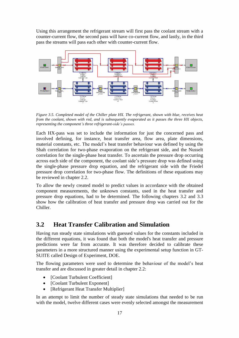
Using this arrangement the refrigerant stream will first pass the coolant stream with a

counter-current flow, the second pass will have co-current flow, and lastly, in the third

pass the streams will pass each other with counter-current flow.

Figure 3.5. Completed model of the Chiller plate HX. The refrigerant, shown with blue, receives heat

from the coolant, shown with red, and is subsequently evaporated as it passes the three HX objects,

representing the component’s three refrigerant-side’s passes.

Each HX-pass was set to include the information for just the concerned pass and

involved defining, for instance, heat transfer area, flow area, plate dimensions,

material constants, etc. The model’s heat transfer behaviour was defined by using the

Shah correlation for two-phase evaporation on the refrigerant side, and the Nusselt

correlation for the single-phase heat transfer. To ascertain the pressure drop occurring

across each side of the component, the coolant side’s pressure drop was defined using

the single-phase pressure drop equation, and the refrigerant side with the Friedel

pressure drop correlation for two-phase flow. The definitions of these equations may

be reviewed in chapter 2.2.

To allow the newly created model to predict values in accordance with the obtained

component measurements, the unknown constants, used in the heat transfer and

pressure drop equations, had to be determined. The following chapters 3.2 and 3.3

show how the calibration of heat transfer and pressure drop was carried out for the

Chiller.

3.2 Heat Transfer Calibration and Simulation

Having run steady state simulations with guessed values for the constants included in

the different equations, it was found that both the model's heat transfer and pressure

predictions were far from accurate. It was therefore decided to calibrate these

parameters in a more structured manner using the experimental setup function in GT-

SUITE called Design of Experiment, DOE.

The flowing parameters were used to determine the behaviour of the model’s heat

transfer and are discussed in greater detail in chapter 2.2:

[Coolant Turbulent Coefficient]

[Coolant Turbulent Exponent]

[Refrigerant Heat Transfer Multiplier]

In an attempt to limit the number of steady state simulations that needed to be run

with the model, twelve different cases were evenly selected amongst the measurement

18

data’s 60 cases. In each of these twelve test-cases, boundary condition data

corresponding to each case was entered in the DOE-setup. Doing so allowed the

optimisation process to find the combination of optimum values best suited to

correlate the simulation data with the measurement points. It was later discovered that

more test-cases could have been included in the optimisation process without

affecting the overall simulation time to any great degree. However, as will be show,

the twelve cases were sufficient to correlate the model to the entire data set.

To calibrate the unknown parameter values the following objective function was

formulated and introduced into the model:

12

0, , )( 2

1

,,

n

QQQQf DataSim

n

i

iDataiSimObj (14)

In equation 14, the term Qsim is the sum of each case’s heat transfer, i.e. the combined

heat transfer from all HX objects in the model, and Qdata is the steady state result for

each case. The simulated heat transfer is then subtracted by the measurement data

belonging to each respective case.

Once these settings were made to the model, numerous steady-state simulations were

run using the DOE plan shown below. The goal of optimisation was specified as

minimising the objective function, and the interval of the test matrix and number of

simulations were set using the Latin Hypercube method, a statistical method for

sampling parameter combinations.

0.1 < [Coolant Turbulent Coefficient] < 1.1

0.01 < [Coolant Turbulent Exponent] < 1.1

0.6 < [Refrigerant Heat Transfer Multiplier] < 2

Number of experiments, i.e. different value combinations, for each test-case:

300

Once the experiments had achieved steady state conditions, the software’s post

processor was used to calculate a response surface for each of the test-cases. Each

response surface is described mathematically by determining how the objective

function depends on the three variables listed above and is created through regression

analysis of the objective function’s steady state results for each case. The process

yields the coefficients to “bowl” shaped quartic functions, fourth degree polynomials,

which are later used when determining which variable values give the smallest

deviation from the actual measurements.

To determine the three single values that would together minimise the deviation from

the actual measurements, and which were at the same time independent of which test-

cases was used, an optimisation was carried out using all the twelve surfaces

simultaneously.

The resulting value combination is as listed:

[Coolant Turbulent Coefficient] = 0.61018

[Coolant Turbulent Exponent] = 0.11361

[Refrigerant Heat Transfer Multiplier] = 1.19999

The newly found physical properties were entered into the Chiller model and the

updated model was used to run new simulations containing the boundary data from

the entire data-set. The results from these simulations are found in the chapter 3.2.1.

19

Due to the matching heat transfer characteristics between the Chiller model and the

data, the current calibration values were decided to suffice for future modelling.

3.2.1 Heat Transfer Results

The heat transfer results from the calibrated chiller model are presented in this

section. Though numerous other results were obtainable, only the total heat transfer

across the heat exchanger was of interest when verifying the results. Depending on how many sub-volumes a model is divided into, it is possible to acquire

simulated values from the in- and/or outlet of each sub-volume. The simulated results

can then be used to compare the quality of the predictions made inside the model with

actual measurement data. For the components investigated in this study no such

detailed measurements had been made and as a consequence the validation was only

carried out at locations in the model were there actually existed physical

measurements.

A graph comparing, steady-state, heat transfer results from the fully calibrated Chiller

model with measured heat-transfer from data-set was can be seen in figure 3.6.

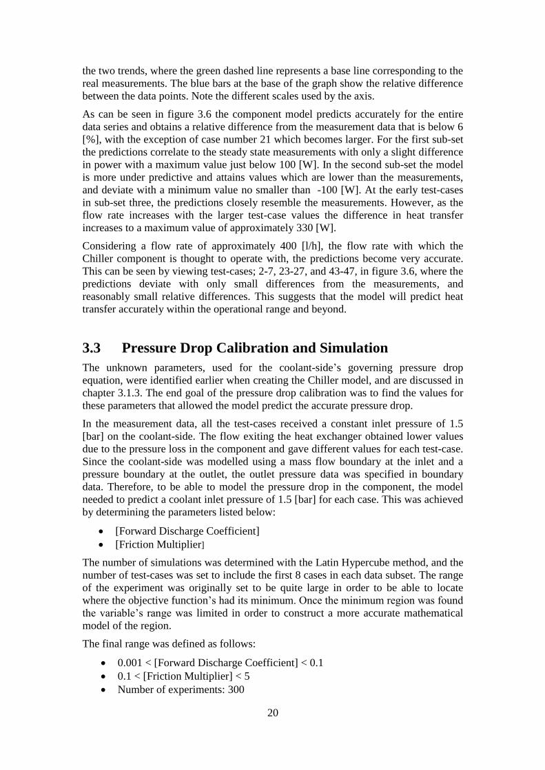
Figure 3.6. Heat-transfer across the component; the simulated steady-state results, blue, are shown in

relation to measured steady-state points, red. Difference between curves, depicted with dashed green

curve, and varying between the black zero line. Note the different scales between left and right y-axis.

Figure 3.6 illustrates how well simulation results retrieved from the model correlates

to measurement data. On the left-axis, indicated with blue, the heat transfer occurring

between the two Chiller streams is shown and measured in units of [W]. These heat

transfer values correspond to the heat transfer occurring in a system during steady-

state conditions. The right-axis, indicated with green, displays the difference between

20

the two trends, where the green dashed line represents a base line corresponding to the

real measurements. The blue bars at the base of the graph show the relative difference

between the data points. Note the different scales used by the axis.

As can be seen in figure 3.6 the component model predicts accurately for the entire

data series and obtains a relative difference from the measurement data that is below 6

[%], with the exception of case number 21 which becomes larger. For the first sub-set

the predictions correlate to the steady state measurements with only a slight difference

in power with a maximum value just below 100 [W]. In the second sub-set the model

is more under predictive and attains values which are lower than the measurements,

and deviate with a minimum value no smaller than -100 [W]. At the early test-cases

in sub-set three, the predictions closely resemble the measurements. However, as the

flow rate increases with the larger test-case values the difference in heat transfer

increases to a maximum value of approximately 330 [W].

Considering a flow rate of approximately 400 [l/h], the flow rate with which the

Chiller component is thought to operate with, the predictions become very accurate.

This can be seen by viewing test-cases; 2-7, 23-27, and 43-47, in figure 3.6, where the

predictions deviate with only small differences from the measurements, and

reasonably small relative differences. This suggests that the model will predict heat

transfer accurately within the operational range and beyond.

3.3 Pressure Drop Calibration and Simulation

The unknown parameters, used for the coolant-side’s governing pressure drop

equation, were identified earlier when creating the Chiller model, and are discussed in

chapter 3.1.3. The end goal of the pressure drop calibration was to find the values for

these parameters that allowed the model predict the accurate pressure drop.

In the measurement data, all the test-cases received a constant inlet pressure of 1.5

[bar] on the coolant-side. The flow exiting the heat exchanger obtained lower values

due to the pressure loss in the component and gave different values for each test-case.

Since the coolant-side was modelled using a mass flow boundary at the inlet and a

pressure boundary at the outlet, the outlet pressure data was specified in boundary

data. Therefore, to be able to model the pressure drop in the component, the model

needed to predict a coolant inlet pressure of 1.5 [bar] for each case. This was achieved

by determining the parameters listed below:

[Forward Discharge Coefficient]

[Friction Multiplier]

The number of simulations was determined with the Latin Hypercube method, and the

number of test-cases was set to include the first 8 cases in each data subset. The range

of the experiment was originally set to be quite large in order to be able to locate

where the objective function’s had its minimum. Once the minimum region was found

the variable’s range was limited in order to construct a more accurate mathematical

model of the region.

The final range was defined as follows:

0.001 < [Forward Discharge Coefficient] < 0.1

0.1 < [Friction Multiplier] < 5

Number of experiments: 300

21

Number of steady state simulations: 8x3x300 =7200

The objective function was formulated in a similar way as to the one used for the heat

transfer calibration, and was defined to measure the simulated versus the measured

pressure drop of each case. The function used coolant pressure values from the inlet of

the model’s first heat exchanger object and outlet pressure from the model’s last heat

exchanger, see equation 15. As with the heat transfer calibration, the intention was to

minimise the objective function in order to find the optimum parameter values which

best described the component’s pressure drop.

2

)()( dataoutinsimoutinObj ppppf (15)

Once the prerequisites for the experiment were entered, the experiments were

simulated in a similar manner as done for the heat transfer calibration. Viewing the

coefficient of determination for the objective function’s resulting regression surfaces

showed that they were unable to accurately predict how the objective function

behaved when varying the Forward Discharge Coefficient and the Friction Multiplier.

Instead of using these surfaces to determine the minimum value of the objective

function, as done for the heat transfer, it was found that the simulation results from the

inlet pressure in the objective function could be used directly to construct new

surfaces that accurately predicted the inlet pressure as a function of the calibration

parameters. The point of doing this was that the inlet pressure function could be used

to optimise towards a target value instead of a minimum or maximum value,

something that had not been considered earlier in this study. The reasons for why the

objective function’s results were inadequate in the regression analysis were not

explored to any further extent.

Finding the correct values for the investigated parameters was done by optimising

with inlet pressure function towards a target of 1.5 [bar], which was the measured

inlet value for all the test-cases.

The optimum values are presented below:

[Forward Discharge Coefficient] = 0.0476

[Friction Multiplier] = 2.8589

The values shown above were introduced into the model and a simulation containing

all the test-cases was run. The pressure results from this simulation are found in the

upcoming chapter 3.3.1.

Since the coolant-side’s heat transfer coefficient is affected by the flow behaviour of

the coolant, the heat transfer results from this simulation was compared with earlier

heat transfer results and found remain virtually unchanged. The calibration on the

coolant-side was therefore deemed to be finished and the attention was instead shifted

to calculating the unknowns on the refrigerant-side.

Calibrating the refrigerant-side’s pressure drop was carried out in a similar manner as

for the coolant-side, however, for this side only a one parameter was identified:

[Friction Multiplier]

The friction multiplier is applied to the Friedel pressure drop correlation for two-

phase flow and is described in more detail in chapter 2.2. The multiplier was modelled

22

with the same value for all the different phase-stages, this assumption that was made

since no other information was available at the time.

Prior to the calibration of heat transfer and coolant pressure drop, the Friction

Multiplier was set to the value of 25 as a result of earlier simulation with the model to

obtain reasonable heat transfer values.

To find a value for the friction multiplier that increased the model’s pressure drop

predictions further, a DOE was set up containing just this one variable and used every

other test-case in the data-set. The interval is specified below:

10 < [Friction Multiplier] < 50

Number of simulations: 10x3x50 =1500

After running the steady-state simulations new quartic response functions were

created using the objective function, equation 15, and the unknown parameter. The

resulting R2-values equalled 1 for all surfaces, and the surfaces were then used for

optimising to minimise the objective function. Doing this the friction multiplier value

32.5 was found. Applying this value to the model, new simulations were run using the

entire data-set to verify if the value predicted pressure drop more correctly.

When comparing the simulation results with the measurement data it was found that

the new value did not fare any better than when using the previous value of 25. In

fact, the new value predicted results that were slightly worse than the previous value.

Due to the need of continuing with the task of modelling the remaining circuit

components, and that the model already predicted accurate heat transfer values, it was

decided to keep the previous value of 25. This decision meant that the model’s heat

transfer did not warrant any new calibration since the heat transfer was found when

using the Friedel correlation with a friction multiplier of 25.

3.3.1 Coolant-Side Pressure Drop Results

Due to the way the model was constructed, the method for calibrating the pressure

drop on the coolant-side was to find the inlet pressure corresponding to 1.5 [bar] for

all the subsequent test-cases. The first graph presented here therefore shows simulated

inlet pressure in relation to a straight line of measurement points, unlike graphs

presented in the earlier chapter concerning heat transfer.

23

Figure 3.8. Simulated inlet pressure, blue, in relation to the constant measured inlet pressure of 1.5

bar, signified with red. The difference between the simulated and measured pressure is indicated by the

green squares and the relative difference is indicated by the blue bars at the bottom of the graph.

Figure 3.8, shows how predicted and measured inlet pressure behave in relation to one

and another. All the simulated values from the optimised model follows the

measurement trends and only deviate from their intended values at the end of each

subset where the coolant flow rate is high. For the third sub-set, where the cases are

simulated with a fixed inlet boundary temperature of 35 [°C], the results show that the

model’s deviation from the measurements is at its largest. Considering the relative

difference in figure 3.8, the model predicts inlet pressures with only minor offsets for

the lower flow rates and with a few percent for the higher flow rates.

The overall results from the calibration show that the coolant pressure drop is very

accurate for most of the test-cases and become slightly less reliable when the flow

increases to high flow rates.

In the following figure, figure 3.9, the accuracy of the pressure drop predictions are

show in relation to the actual pressure drop.

24

Figure 3.9. Coolant-side pressure drop predictions versus pressure drop measurements. The pressure

drop is shown in three graphs corresponding to the three data sub-sets.

In the figure 3.9 the exponential proportionality of the pressure drop to the flow rate

becomes apparent. The results also indicate that the model’s behaviour correlates to

the measurements with only small deviation. Observing figure 3.8 anew, and viewing

the last points in each of the simulated trends it is possible to see that the model over-

predicts the inlet pressure. When considering the pressure drop, this over-prediction is

corrected for by simulated outlet pressures which are slightly higher than the

measured outlet pressure. When subtracting the simulated inlet pressure with the

outlet pressure the resulting pressure drop correlated to the measurement data. The

largest difference between simulated and measured pressure drop is, for each subset,

and in subsequent order: 0.0188 [bar] for case 17, with a flow rate of 1700 [l/h],

0.0191 [bar] for case 37, with a flow rate of 1700 [l/h], and 0.0186 [bar] for case 60,

with a flow rate of 2000 [l/h].

3.3.2 Refrigerant Pressure Drop Results

The results from running steady-state simulations with the entire dataset whiles using

a friction multiplier of 25 are shown in this section. As reasoned earlier, this value

was favoured instead of the value that was found during the calibration of the

refrigerant-side. The refrigerant-side’s inlet pressure is shown in figure 3.10 for both

simulation and empirical data. As opposed to coolant-side, the inlet pressure boundary

condition was not held constant, and instead allowed to vary depending on the test-

case.

25

Figure 3.10. Refrigerant inlet pressure; simulated Steady-State results in relation to measurement data.

The difference between curves is shown with green squares and the relative difference with blue bars at

the base of the graph. Note the different scales between the different axis.

Figure 3.10 indicates that the best correlation occurs in the second subset. In this

subset the refrigerant boundary conditions contains a constant back pressure of 4

[bar]. In subsets one and three, with back pressures of 3 and 4 [bar] respectively, the

largest deviations occur at the higher case numbers and in subset two the largest

difference occurs almost at the beginning of the set.

Viewing the first subset first, the model over-predicts inlet pressure from cases 1-6

and then under-predicts for cases 7-20. The difference between simulated results and

that of the test-data varies between, 0.07 [bar] to -0.22 [bar], minus indicating under

predictions. The largest difference occurs at the last test-case, with a value of -0.22

[bar].

Considering the second subset the model predicts more accurately than in the first and

third subset. In this set the difference between simulated and actual values is no more

than 0.1 [bar]. In the third subset the simulation-trend starts to deviate from the

measurements with increasing test-case values and making predictions that become

more and more under-predicted. The maximum deviation that occurred in this subset

contained a difference of -0.48 [bar].

As seen by the difference in behaviour between the tree subsets, the overall trend for

the inlet pressure is not fully captured by the model. Any use of the model for

accurate inlet pressure predictions becomes questionable for the higher flow rates.

However, for lower flow rates closer to the Chiller’s operational region,

approximately 400-500 [l/h], the predictions are more accurate. In this region the

relative difference is below 2 [%], see figure 3.10.

The graphs in figure 3.11 show how refrigerant-side’s pressure drop predictions

behave in comparison to measurement data. In these graphs the pressure drop is

26

depicted in scatter plots with refrigerant mass flow on the x-axis, this in contrast to

earlier graphs which were presented using test-cases.

Figure 3.11. Pressure drop on the refrigerant side. The blue curve indicates simulation data and the

red curve indicates measurement data.

In figure 3.11 the model's inadequacy to correlate the pressure drop across the

refrigerant-side becomes apparent. As seen, the simulated pressure drop does not

follow the measurement trends completely and is both under and over predictive.

In the intended range of operation, where the coolant flow is between 400-500 [l/h],

the refrigerant mass flow rate corresponds to the following intervals; first subset; 60-

70, second; 35-40, third; 90-105 [kg/h]. In these intervals the model predicts values

that are not too far from the pressure drop measurements and the model's behaviour

can be said to be sufficiently accurate in this region. This can also be seen when

viewing cases; 4-5, 24-25 and 44-45 in figure 3.10.

3.4 The External Heat Exchanger

The External Heat Exchanger is placed on the vehicle’s extremities and exchanges

heat with the surrounding air, thereby cooling the circuit when ambient temperatures

are agreeable. Schematically, the heat exchanger is connected to the circuit between

the pump and before the Chiller, see figure 1.1 for schematic layout. In addition to the

heat exchanger, a bypass-connection was added to allow the cooling-fluid to pass

either through the External HX in combination with the Chiller, or through the Chiller

separately. This configuration enables the system to become flexible in its choice of

cooling method. Furthermore, this configuration avoids unwanted pressure loss by

having the option of bypassing the External HX, as opposed to letting the fluid pass

through the component continually.

The modelled External HX component is comprised of two main parts; an axial-fan,

and a tube-and-fin heat exchanger, as reference one might consider the design of the

condenser used for engine cooling which exists in the vast majority of cars today. The

axial-fan is placed in front of the exchanger and may be run separately, or as a

complement to the Chiller during conditions with lower ambient temperature.

27

3.4.1 External Heat Exchanger Modelling

The simpler design and flow scheme of the external heat exchanger, in comparison to

the Chiller, made it possible to use a more straightforward modelling method. By

connecting the primary and secondary sides to a single heat exchanger object the

component’s performance could be defined using lookup tables. The tables, in turn,

contained information concerning the two sides’; heat transfer, pressure drop, and

temperature, as dependent on each side’s inlet flow, and was collected from the

components data-set. A description of the tube-and-fin layout and dimensions was

included using various geometry parameters.

Modelling the heat exchanger in this way ensured that the component would provide

correct information concerning heat transfer, as well as, flow characteristics for the

flow range specified in the data-set.

Figure 3.12, below, shows the final version of the component’s model. In this

representation of the model the coolant-side's in- and outlet boundary conditions have

been removed and are instead joined directly to the remaining cooling system. The

objects placed in front of the air-side inlet, seen at the bottom of figure 3.12, are the

fan object, the fan’s control system, and an air-ram inlet boundary.

Figure 3.12. Schematic overview of the External Heat Exchanger’s system.

The system’s fan component was obtained from the component library included in

GT-SUITE. This object models an axial fan by creating a fan characteristic map of

performance measurements carried out earlier on a fan. For the axial fan used in this

study no easily accessible measurement data was available. Instead a rudimentary

graph of the fan's behaviour was used to extract data points. This was done by writing

a MATLAB script which enabled data to be collected by manually selecting points on

the graph.

Evaluating the heat exchanger's heat transfer and pressure drop performance was done

by running seven separate steady state simulations and comparing the simulated

results with measurements at the component's in- and outlet. The seven sets of

boundary conditions were assumed to be sufficient for determining the models

accuracy.

28

3.4.2 External Heat Exchanger Model Results

In this section the simulated results of the modelled component's performance is

presented for the seven different sets of boundary conditions. In the boundary sets

used, the flow rates for both sides of the component are increased for every

subsequent test-case. The boundary conditions for the outlet pressures and inlet

temperatures also used the same data as the measurements of that set. Below, in figure 3.13, the total heat transfer occurring across the component is

compared between the simulated and measured values. The difference between the

values belonging to a single test-case is shown with green boxes in figure fafdsa, and

the relative difference is indicated by the blue bars at the bottom of the graph. Note

the different scales used for the axis.

Simulation was conducted using seven test-cases with different boundary conditions.

The boundary conditions flow rates were increased for every subsequent test-case,

and the other performance conditions are also increased between the test-cases.

Below, in figure 3.13, the simulated heat transfer from the External heat exchanger is

shown in relation to the components measurement data.

Figure 3.13. The External Heat Exchanger’s heat transfer trends; simulated Steady-State results in

relation to measurement data. The difference between curves is shown with green squares and the

relative difference with blue bars at the base of the graph. Note the different scales between the

different axis.

As expected, the heat transfer behaviour emulates that of the measurements made on

the component and predicts values reasonably close to its mark. The largest relative

difference is observed for case 1 where the relative difference amounts to almost 15

[%] with a difference in power of roughly 70 [W]. Viewing the remaining cases it is

possible to see that the relative difference resides under 7 [%], and looking back at the

heat transfer results from the Chiller component in chapter 3.2.1, the relative

difference never exceeded 6 [%], with the exception of case 21. By comparing the

results from the two component models it was seen that the External heat exchanger

29

received a similar level of accuracy as that of the Chiller. It was therefore decided to

proceed with the evaluation rather than trying to improve on the results.

Since the model was given measurements data to interpolate from when finding

values for the heat transfer and pressure drop it is justified to wonder why the results

do not become entirely accurate. The discrepancy is caused by the model's inability to

capture all the flow related phenomena, and is a consequence of the trade of between

accuracy and computational demand. This limitation leads to slightly inaccurate input

values when using the lookup table to find values for heat transfer and pressure, as

discussed in the preceding text. Another contributor to decreasing the models

accuracy is the lookup table itself, were the model used linear interpolation between

two measured values.

The upcoming figure, figure 3.14, illustrates how the pressure drops of both streams

behave in comparison with actual measurements. Not the difference units of pressure

on the y-axis.

Figure 3.14. shows the heat exchanger’s predicted pressure drop in relation to actual measurements

for both the air-side and coolant-side.

Viewing the results from of the pressure drop for the air-side and the coolant-side

figures 3.14, it is possible to see that the pressure drop predictions correlated better to

the measurements for the air-side than for the coolant-side. The maximum deviation

for the air-side predictions is 18 [Pa] and occurs at test-case 7. For the coolant-side the

maximum deviation is approximately 14 [kPa], and also occurs at the seventh test-

case. The relative difference, between simulated data and measurement, is largest at

the beginning of the both the air-side and coolant-side trends, and then decreases with

increasing test-case numbers. For the air-side the largest relative difference is found in

the first point, with a value of 18.5 [%]. The largest relative difference for the coolant-

side is found at the second point, having a value of 28 [%]. Although the pressure

drop predictions made by the model are less accurate than those of the Chiller, the

decision was taken to continue onwards with the remaining components of the circuit.

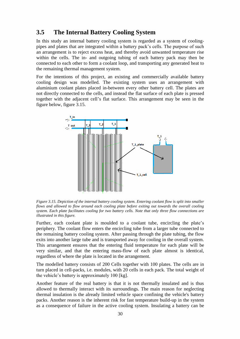
30

3.5 The Internal Battery Cooling System

In this study an internal battery cooling system is regarded as a system of cooling-

pipes and plates that are integrated within a battery pack’s cells. The purpose of such

an arrangement is to reject excess heat, and thereby avoid unwanted temperature rise

within the cells. The in- and outgoing tubing of each battery pack may then be

connected to each other to form a coolant loop, and transporting any generated heat to

the remaining thermal management system.

For the intentions of this project, an existing and commercially available battery

cooling design was modelled. The existing system uses an arrangement with

aluminium coolant plates placed in-between every other battery cell. The plates are

not directly connected to the cells, and instead the flat surface of each plate is pressed

together with the adjacent cell’s flat surface. This arrangement may be seen in the

figure below, figure 3.15.

Figure 3.15. Depiction of the internal battery cooling system. Entering coolant flow is split into smaller

flows and allowed to flow around each cooling plate before exiting out towards the overall cooling

system. Each plate facilitates cooling for two battery cells. Note that only three flow connections are

illustrated in this figure.

Further, each coolant plate is moulded to a coolant tube, encircling the plate’s

periphery. The coolant flow enters the encircling tube from a larger tube connected to

the remaining battery cooling system. After passing through the plate tubing, the flow

exits into another large tube and is transported away for cooling in the overall system.

This arrangement ensures that the entering fluid temperature for each plate will be

very similar, and that the entering mass-flow of each plate almost is identical,

regardless of where the plate is located in the arrangement.

The modelled battery consists of 200 Cells together with 100 plates. The cells are in

turn placed in cell-packs, i.e. modules, with 20 cells in each pack. The total weight of

the vehicle’s battery is approximately 100 [kg].

Another feature of the real battery is that it is not thermally insulated and is thus

allowed to thermally interact with its surroundings. The main reason for neglecting

thermal insulation is the already limited vehicle space confining the vehicle's battery

packs. Another reason is the inherent risk for fast temperature build-up in the system

as a consequence of failure in the active cooling system. Insulating a battery can be

31

used to decrease the energy demand of the cooling system, thereby increasing vehicle

range. In circumstances where ambient temperature is higher than battery cell

temperature, insulating the battery becomes a desirable option in order to limit the

heat transfer into the battery.

The link between the battery system and its surroundings was not studied further in

this study. However, as will become evident later, the effects of thermal heat pick-up

are definitely noticeable.

3.5.1 Internal Battery Cooling System Modelling

Modelling of the internal battery cooling system was done by initially constructing the

two main coolant streams connecting the system to the remaining cooling circuit.

Since these tubes were to be connected to the all the cooling plates they were

modelled using numerous tube objects which each allowed the stream to use three

flow connections. As the stream passes through an object a portion of the fluid leaves

the tube in a third perpendicular connection whiles the remaining fluid continues in

the main flow direction. The third, perpendicular, connection is then connected to a

cooling-plate, and the fluid exiting the tube in the main flow direction continues into

the next three-way object. Modelling in this way allowed the internal system’s flow to

be arranged as described in the previous text.

To assemble the coolant-plates, surrounding tubing, and battery cells, a new

modelling method was attempted. The method entailed combining one plate with two

cells into a compound-object and by doing so the process of modelling all 200 cells

became simpler. Constructing the compound-object was done by adding two thermal-

mass objects, representing the cells, and linking these masses to a circling

arrangement of tube-objects. The tube-objects were then, in turn, linked to yet another

thermal-mass, representing the thin aluminium coolant-plate. Figure 3.16, shows how

these objects were connected to resemble the sub circuit.

Figure 3.16. shows how the cells, coolant plate, and encircling tubes were modelled. The cells, seen to

the right and left in the figure, are connected via a thermal link to the plate object which is, in turn,

connected to the encircling tubes. The incoming coolant is then transported around the thin plate

object and removes any excess heat.

A thermal-mass object is essentially a mass which may accumulate and transfer

energy. The object also contains information regarding geometries and dimensions of

the mass, the heat capacity of the object, and may be specified to include information

concerning possible heat-rate/heat-flux into the object of adjacent temperature

boundaries. Linking this object to another object allows for energy transfer to be

calculated though the body via conduction. In order to determine how heat is

conducted through the object, more specifications have to be made in each thermal-

32

mass. Here, material properties like thermal conductivity, density, and specific heat

have to be defined alongside with the mass-object’s dimensions. In the compound

shown in figure 3.16, three thermal-mass objects were modelled to represent the two

cells and one cooling plate. These objects were linked together using the dimensions

of their corresponding plane surfaces, and it was assumed that the contact area

between these objects was perfect and permitting heat transfer to occur across the

entire surface. This may not be the case for actual applications, since the cells must be

allowed to expand and contract, resulting in different contact areas between the cell

and plate. Continuing onwards, the cooling plate was linked to the surrounding tubes

using the plate’s short side geometries. Any heat transfer from the plate is then led

through the encircling tubes to the fluid by convection.

Having created a compounded-object containing one cell and two coolant plates, the

remaining cells and plates were easily arranged in battery packs. Figure 3.17,

illustrates how the first out of 10 battery packs were modelled. This arrangement was

repeated until 200 cells were connected to each other, forming the internal battery

cooling system.

Figure 3.17. The Internal Battery Cooling System’s component model. The model consists of 10 cell

packs each with 20 cells and 10 cooling plats, here only one such pack is shown. To the left; inlet and

outlet boundaries for the coolant.

Evaluating how well the model resembled the real component became challenging

since only a limited amount of test-data existed on the behaviour of the hybrid

vehicle’s internal battery cooling. Numerous measurements had been made on overall

vehicle performance, but regarding the internal battery cooling, only measurements on

inlet and outlet temperatures and mass-flow had been made. Moreover, the data that

existed had almost explicitly been obtained during transient conditions, meaning that

no steady-state measurements were available. This meant that the model’s reliability

had to be asserted using transient simulation with boundary conditions which varied

with time. This being said, the only quantities usable for validation were time

dependent temperature measurements made at the in- and outlet of the internal battery

cooling system, as well as in some cases, the coolant mass flow. Since the heat

capacity of the coolant was known, it was possible to calculate heat transfer occurring

across the system. When viewing the measured heat transfer values it was found that

the vehicle test-data had been measured under conditions where the electrical

drivetrain had not been in use. Instead, propulsion had been supplied by the hybrid’s

other drivetrain, i.e. its internal combustion engine. This meant that no thermal energy

was generated through battery discharge, and that the measured cooling requirement

was caused by other sources of heating, such as external heat transfer into the system.

Lacking cell temperatures made it difficult to know what initial condition the system

was in at the beginning of the sequence. To circumvent this, the initial-state

33

temperatures, of the coolant and thermal masses, were estimated to be a few degrees

higher than the fluid’s initial outlet temperature.

The three calibration parameters shown below were chosen because they were thought

to to affect heat transfer of the system the most, and, once calibrated, be able to make

the model match the behaviour of the transient cool-down sequence:

[Tube - Heat Transfer Multiplier]

[Cell Mass]

[Plate - Tube Area Heat Transfer Multiplier]

The first parameter, the Tube – Heat Transfer Multiplier, is a multiplier which affects

the heat transfer between the tube wall of the tube encircling the plate and the fluid

flowing thorough the tube, see chapter 2.2 for more information on heat transfer. The

second parameter is a mass term which was selected because of the uncertainties

attributed the initial level of thermal energy stored in the overall mass of the battery

and its cells at the start of the measurement sequence. The accumulated energy is

determined by the initial temperature of the materials, the heat capacity of each

material, and the total amount of mass. Due to uncertainties regarding all these

quantities found in the data, it was reasoned that different cell masses hade to be

tested in order compensate for these factors. The premise was that the cell mass

should not differ too much from the actual mass of the cells, which accounted for

most of the battery’s mass. The parameter listed last represents the area connecting

the coolant-plate to its encircling tubing. Due to the plate being pressed onto the tubes

it was difficult to ascertain the actual contact area, and it was therefore decided to

include this parameter as an unknown in the calibration process.

The calibration was carried out in a similar manner as was done for the previous

components. To measure how well each set of tested parameter values performed, a

temperature dependent objective function was formulated. This function resembled

those used earlier in this study but was set to use outlet temperature as its variable

instead of heat transfer or pressure drop. Since the simulations and measurement data

were transient, instead of steady state, the objective function used the averaged outlet

temperature of the entire sequence when comparing a simulation's temperature with

the measured temperature. As opposed to the steady-state simulations used earlier in

this project, a transient simulation is time dependent. It is therefore not just a question

of finding the steady-state end results from a simulation, but instead using results

from each time step. In this case it was important to investigate the temperature

behaviour at the in- and outlet, and it therefore became necessary to use the

information in each time-step when employing the objective function. To accomplish

this, a moving average component was connected to the objective functions output.

The moving average then computes an average of all the objective function’s values

stored for each time-step. Having done this ensures that the calibration parameters

optimum values are found, and which give the smallest averaged difference between

the simulated sequence and the measured sequence.

The simulations were designed systemically using the DOE method to find the

optimum values for the tube's heat transfer multiplier, the cell mass, and the heat

transfer multiplier associated with the cell's plate and connecting tubing. Having

carried out the simulated experiments the surface fits, i.e. mathematical models, were

found to be slightly less reliable then normally desired, but were decided to be

sufficient for the purposes of at least an initial surface optimisation to find the values

for a minimum objective function. Using the quartic regression option available in

34

DOE-POST, the mode attained an R2-value of approximately 0.9. Including all the

response surface models in one single optimisation, a value-combination was found

with a corresponding objective function value of approximately 0.08, i.e. the squared

error between the simulated- and measured curve.

The intervals used for the DOE are listed below together with best calibration values:

[Tube - Heat Transfer Multiplier] = 3.4548 { 0.1 – 10 }

[Cell Mass] = 938 [g] { 100 – 1500 }

[Plate - Tube Area Heat Transfer Multiplier] = 0.6875 { 0.2 – 1.5 }

Having found optimum parameter values, a new simulation was run using a longer

transient sequence containing both cooling and heating episodes. This data-set was

obtained from a different component test carried out with the hybrid vehicle during

different conditions. It was found that the model now correlated well with the test

data, and no further modelling of the internal battery cooling system was deemed to

be required. Due to the model's ability to accurately predict in-and outlet temperatures

it is also by extension able to accurately predict heat transfer occurring across the

system. Furthermore, any temperature and heat transfer predictions made within the

system are also deemed to be within reason. This was however not possible to validate

du to the limited measurement data.

Applying a thermal load may be done in the model’s battery cells by specifying a cell-

specific heat output. Doing this may be regarded as simulating with a system that

actively uses the vehicles battery. The heat output may further be modelled as a time

dependent, allowing the cells to output residual heat in a way that follows real life

behaviour, accounting for instance for ramping heat output during tasking

accelerations.

The results from simulation with the calibration data-set, using the best fitting

calibration values, and simulation with the validation measurement data, are presented

and discussed in the chapter, chapter 3.5.2.

3.5.2 Internal Battery Cooling Model Results

In this chapter the results from the transient simulations are presented. The results

give insight in how the entire battery behaves when being cooled, or heated, during

various inlet temperatures. During the process of determining the calibration

parameter's values, the model was set to use measured sequences containing variable

inlet temperature and mass flow sequences when simulating. Both these sequences

were obtained from the actual measurements and included in the model as lookup

tables.

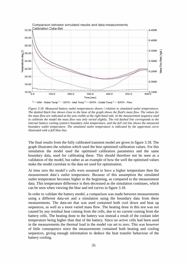
35

Figure 3.18. Measured battery outlet temperatures shown i relation to simulated outlet temperatures.

The dashed black line shown close to the base of the graph shows the fluid's mass flow. The values for

the mass flow are indicated at the axis visible at the right hand side. In the measurement sequence used

to calibrate the model the mass flow was only varied slightly. The red dashed line corresponds to the

internal battery cooling system's boundary inlet temperature, and the full red line shows the measured

boundary outlet temperature. The simulated outlet temperature is indicated by the uppermost curve

illustrated with a full blue line.

The final results from the fully calibrated transient model are given in figure 3.18. The

graph illustrates the solution which used the best optimised calibration values. For this

simulation the model used the optimised calibration parameters and the same

boundary data, used for calibrating these. This should therefore not be seen as a

validation of the model, but rather as an example of how the well the optimised values

make the model correlate to the data set used for optimisation.

At time zero the model’s cells were assumed to have a higher temperature then the

measurement data’s outlet temperature. Because of this assumption the simulated

outlet temperature becomes higher in the beginning, as compared to the measurement

data. This temperature difference is then decreased as the simulation continues, which

can be seen when viewing the blue and red curves in figure 3.18.

In order to validate the battery model, a comparison was made between measurements

using a different data-set and a simulation using the boundary data from these

measurements. The data-set that was used contained both cool down and heat up

sequences, as well as a more varied mass flow. The heating done in this test was not

caused by any residual heat coming from the cells, due to no current coming from the

battery cells. The heating done to the battery was instead a result of the coolant inlet

temperature being higher than that of the battery. Since no active cells had been used

in the measurements the thermal load in the model vas set to zero. This was however

of little consequence since the measurements contained both heating and cooling

sequences, giving enough information to deduce the heat transfer behaviour of the

battery cooling.

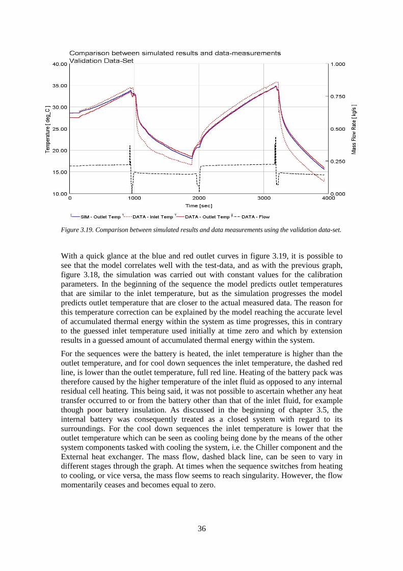
36

Figure 3.19. Comparison between simulated results and data measurements using the validation data-set.

With a quick glance at the blue and red outlet curves in figure 3.19, it is possible to

see that the model correlates well with the test-data, and as with the previous graph,

figure 3.18, the simulation was carried out with constant values for the calibration

parameters. In the beginning of the sequence the model predicts outlet temperatures

that are similar to the inlet temperature, but as the simulation progresses the model

predicts outlet temperature that are closer to the actual measured data. The reason for

this temperature correction can be explained by the model reaching the accurate level

of accumulated thermal energy within the system as time progresses, this in contrary

to the guessed inlet temperature used initially at time zero and which by extension

results in a guessed amount of accumulated thermal energy within the system.

For the sequences were the battery is heated, the inlet temperature is higher than the

outlet temperature, and for cool down sequences the inlet temperature, the dashed red

line, is lower than the outlet temperature, full red line. Heating of the battery pack was

therefore caused by the higher temperature of the inlet fluid as opposed to any internal

residual cell heating. This being said, it was not possible to ascertain whether any heat

transfer occurred to or from the battery other than that of the inlet fluid, for example

though poor battery insulation. As discussed in the beginning of chapter 3.5, the

internal battery was consequently treated as a closed system with regard to its

surroundings. For the cool down sequences the inlet temperature is lower that the

outlet temperature which can be seen as cooling being done by the means of the other

system components tasked with cooling the system, i.e. the Chiller component and the

External heat exchanger. The mass flow, dashed black line, can be seen to vary in

different stages through the graph. At times when the sequence switches from heating

to cooling, or vice versa, the mass flow seems to reach singularity. However, the flow

momentarily ceases and becomes equal to zero.

37

3.6 The Radial Pump

A key component in the studied closed system is the pump. The pump is tasked with

increasing fluid pressure so that the fluid constantly is in motion. The component’s

design therefore needs to be able to compensate for the pressure drop occurring

throughout the system’s different parts, as well as, ensuring a satisfactory flow rate

that complies with the systems need to extract heat from the battery component. The

pump used in this system has a maximum rotational speed of 6000 rpm and is capable

of raising the pressure with a differential pressure of approximately a 0.75 [bar]. The

power requirements of the pump are seemingly small and never exceed 80 [W].

The characteristics of the real component were obtained by collecting data points

from a pump characteristic map acquired from the manufacturer of the pump.

Collecting the data was done in a similar manner as for the External heat exchanger

using a MATLAB script and manually collecting the information The resulting

characteristic map depicts a contour plot of the pressure rise and the volume flow on

the y- and x-axis respectively, and as functions of the pump's rotational speed. The

contour graph for the system's pump is presented in figure 3.21 and is discussed later

in this section. The schematic representation found in figure 3.20 below shows the final model of the

component. The pump object is shown in the centre of the figure and illustrated with a

circle containing an arrow. In this object information which describes the pump's

behaviour is entered in lookup tables which in turn contain properties like pressure

rise, volume flow, rotational speed, efficiency, and power requirements. In order to

determine the amount of work done by the pump, the model finds the required rise in

pressure the pump needs to supply to compensate for the pressure losses occurring

throughout the system. Consequently both the pressure rise and volume flow of the

system is determined by which rotational speed is set to the pump, and through this

the actual power requirements may be determined.

Figure 3.20. Overview of the radial pump model.

The figure 3.21, below, illustrates the pump characteristic map for the radial pump for

both the modelled and real component. This map provides details about the pressure

rise and the volumetric flow rate, corresponding to a rotational speed, shown with

38

dashed lines. Also included in the map, is the pump’s efficiency presented with

contour lines, or islands. These efficiency islands show that the pump can reach a

maximum efficiency of 37 [%] during operation with a rotational speed of 6000 [rpm]

and a system pressure drop of approximately 0.65 [bar]. Furthermore it should be

stated that the model’s map is presented here using a limited number of efficiency

contours to avoid making the plot to complex, however, when used for simulation will

efficiency be interpolated using more contour lines.

Figure 3.21. The system’s pump characteristic map.

To illustrate how the pump is used in the system, two system curves were

incorporated onto the modelled map. These curves are shown in figure 3.21, using a

red or a blue curve, and correspond to two different situations. The blue line illustrates

pressure drop throughout the system as a function of volume flow, during a situation

where the External Heat Exchanger is active. The red line shows the circuit’s pressure

drop when the External Heat Exchanger is being bypassed, and as a consequence the

pressure-drop in the system will become slightly smaller. Regardless of operations

with or without the External heat-exchanger, the pump efficiency becomes very small,

approximately 10%.

39

4 Circuit Modelling

An integral part of the component modelling presented so far in this thesis work was

to ensure a high level of accuracy for each individual component. Doing this made it

possible to produce a good representation of the entire battery cooling system which

in turn could be used to investigate the complicated interplay between the system’s

various parts.

Forming the complete battery cooling circuit was done by joining the separate

component models with tubes of different dimensions and arranging them as shown in

the system’s overview, figure 1.1, chapter 1.1. The connecting tubes were constructed

by importing computer aided design, CAD, schematics into GT-SUITE, and thereby

enabling the model to use correct circuit dimensions and geometries for future

computation.

To make complete circuit more manageable, all main component models were

arranged into subassemblies. The assemblies were then connected to the remaining

circuit by linking each assembly to its corresponding in- and outlet pipe. The resulting

circuit is presented below in figure 4.1.

Figure 4.1. Illustration the final model of the battery cooling system.

To decrease pressure fluctuations in a closed loop system, an accumulator tank is

often integrated into the circuit. Pressure fluctuation may be cause by density

variations in a working fluid, often as a result of heating and cooling. Usually the

variation in pressure is fairly small, but can in severe cases lead to pipe breakage if

left unchecked.

41

5 Control Strategy

To advocate decreased energy usage in the cooling system, a study on the control of

the system was conducted. The overall approach was to find control methods that

would moderate energy consumption in the system by controlling the system’s

different energy consuming components in a satisfactory way. Further, this strategy

should be seen as more of an example of what 1D simulation may accomplish, rather

than a complete control strategy of the circuit’s behaviour. It is naturally possible to

increase the complexity of the analysis and account for more constraints on the

control strategy, such as including vapour quality exiting the Chiller, or quicker cool

down sequences due to larger heat transfer. The strategy was, however, limited in this

thesis to investigating the most optimal cooling method from an energy efficiency

point of view.

The components that require energy input in the battery cooling system are the fan in

the External heat exchange, the pump, and indirectly the AC-system’s compressor.

The AC-system is connected to the battery cooling system through the Chiller, which

heat exchanges with the AC-system’s refrigerant. Any cooling done by the Chiller

therefore requires additional compressor work. Determining the most efficient way to

cool the battery therefore involves investigating the interplay between the

performance of energy consuming components and circuit. Doing such a task without

CAE becomes challenging, and to promote the work done earlier with constructing

the transient model, the model was used in the process of finding an energy efficient

control strategy.

Finding optimal ways of controlling these components, during various operational

conditions, was done by firstly determining a way of measuring how efficiently

cooling was done in the system. The chosen approach was to measure the Coefficient

of Performance, COP, of the cooling system during various fixed cell and ambient

temperatures. The COP function was defined as show below in the equation 3, below.

PumpFanComp

EXChiller

PPP

QQCOP

(16)

Since heat was extracted through both the Chiller and External heat exchanger, the

heat transfer leaving these components was places in the nominator of the equation. In

the denominator, the power consumption of the three consumers was summed. Using

this way of measuring made it possible to ascertain how energy efficient the cooling

was performed using a single component, or a combination of components.

To determine the best way of cooling the battery cells, a test plan was formed. The

overall approach involved investigating the COP value of the system during a specific

cell temperature and a specific ambient temperature together with various setting for

the power consuming components. Using this method made it possible to predict the

best way of using the system components for a given cell temperature and under a

certain ambient temperature. To elaborate further, this method answered the question

on how to cool the battery cells in the most energy efficient way, during operations

with a certain cell temperature and a given ambient temperature. Furthermore, the

method allowed investigating whether it was most efficient to use the same settings

during a cooling sequence, or if it was preferable to us an adaptive system which

changed cooling method as the temperature in the cells decreased.

42

In the cooling analysis, a number of parameters were chosen to describe the energy

consumption of each component. For the AC-system’s compressor this involved

determining which parameters affected power consumption. To predict how the AC-

system affected the heat exchange in Chiller, and the power consumption of the

compressor, responses from an AC-system’s model were used. This gave the power

consumption of the entire AC-system, as dependent on the variables; ambient air

temperature and rotational speed. To simplify the complex nature of the AC-circuit, a

system setting was chosen were only the Chiller demanded cooling in the system.

This meant that no other cooling was demanded by the AC-circuit and is equivalent of

saying that no vehicle cabin-air conditioning was done. This limitation was posed due

to the limited time frame of the thesis.

The other power consuming components were already integrated in the battery

cooling model. The power consumption of the system’s pump was determined by

rotational speed and was included as a parameter to be varied. The External HX’s

power usage was predicted by both ambient air temperature and rotational speed. To

simplify the study, the fan did not account for overblown conditions caused by a

vehicle in motion. This can result in slightly less energy being demanded by the fan,

due to the fan being aided in cooling the HX by air already in motion. This limitation

was posed due to the limited time frame of this study.

To find the COP value for each combination of cell temperature and ambient

temperature, the system had to be simulated to steady-state with the desired cell and

ambient temperature. To achieve this, the cells in the compound objects, described in

chapter 3.5.1, were modified to have a constant temperature boundary corresponding

to the tested cell temperature and thereby giving all the cells a uniform temperature.

Additionally the mass of each cell was removed to decrease thermal inertia and

increase the computational speed to reach steady-state results.

Once the changes discussed above were made to the circuit model, it was possible to

proceed with the analysis. To make the experiment more manageable the analysis was

divided into three overall cases. The first case tested all the different variable

combinations of cooling the battery with both the Chiller and the External HX. The

second case investigated the same combinations but when only using the Chiller

component and bypassing the External HX. The last case used only the External HX

and the Chiller was excluded by setting the refrigerant side’s mass flow to zero.

Designing the experiment for the different simulations was done using the DOE

method. The objective function in the experiment was set as the COP, and the

parameters that varied are listed below together with their intervals. Note that not all

the listed variables were used in each case, as discussed in the preceding text.

Imposed Cell Temp {15 – 50 °C}

Ambient Temperature {15 – 40 °C}

Compressor Speed {600 – 2500 rpm, or not used}

Fan Speed {100 – 3600 rpm, or not used}

Pump Speed {600 – 6000 rpm}

The test matrix was constructed using the Latin Hypercube method and contained 500

experiments for each of the three cases. The compressor speed’s lower limit was set to

600 [rpm] and not zero due to restrictions in the AC-system. For the fan- and pump

speed it was found that the solver experienced difficulties converging when no air or

coolant flow was used, hence the speeds’ lower limit was set to 100 [rpm] and 600

43

[rpm] respectively. To exemplify how the simulations were carried out, the first of

these 500 simulations was set to contain an ambient temperature of 25.2 [°C], a cell

temperature of 15.5 [°C]. The rotational speeds were set to 1400, 3360, and 1152

[rpm], relating to the list.

Once all the simulations were completed the results from each case were viewed in

the program’s post processer and used to construct a response surface of the

coefficient of performance for each case. The trustworthiness of the response surfaces

was assessed using the coefficient of determination, the R2-value, which became 0.94

for case one, 0.8 for case two, and 0.92 for case three. Considering these values it was

decided to exclude the results of case two from the analysis, this since the value of 0.8

was deemed to be too low. The decision was also made with the knowledge that the

behaviour of second case’s strategy was captured to some extent in the first case.

Thereby still giving important information regarding when to use the Chiller and

when to not.

Determining the most efficient way of cooling the system during different temperature

conditions was done by optimisation on the response surfaces. For the first case this

involved maximising the COP function using the three speeds as independent

variables, and setting the ambient and cell temperature to fixed values. The

optimisation for the third case was done in a similar manner, but did not include the

compressor speed as an independent variable.

5.1 Control Strategy Results

In this section the results from the control strategy’s optimisation and analysis are

shown and discussed. The optimum way of cooling the battery is shown here from an

energy efficiency point of view and the results were initially collected from steady-

state simulations using given ambient- and cell temperatures. The results were then

analysed in DOE post processer using regression analysis to create surfaces, and

thereafter used for optimisation in order to provide an answer to the question: Which

are the cooling system’s optimum energy efficiency settings for cooling the battery

cells, given a certain cell temperature and during a given ambient temperature?

In figure 5.1 an example of a response surface is shown. The surface was created from

simulations using only the External HX component for cooling. In this case a cell

temperature of 40 [°C] and an ambient temperature of 15 [°C] were used. Using this

surface it was possible to investigate how the system’s COP varies when applying

different rotational speeds for both pump and External HX fan. The figure also reveals

that during these circumstances, an optimum COP-value is found when using a pump

speed of ~3700 [rpm] and a fan speed of ~1300 [rpm].

44

Figure 5.1. shows how the system’s coefficient of performance behaves when the fan’s and pump’s

rotational speeds are altered. This surface model was created from simulation results when using the

External HX separately to cool the cells during the following boundary conditions; cell temperature at

40 [°C] and an ambient temperature at 15 [°C].

The results presented in figure 5.2 below, show the optimum COP-value for each

investigated ambient temperature and cell temperature. The figure also illustrates

which cooling component was used during a given situation and is indicated by the

following numerals; 1, for Chiller, and 2, for the External HX. To be able to relate

how well the optimum solutions performed, a reference control strategy was

constructed, see the bottom part of figure 5.2. This strategy was designed to use

maximum rotational speeds for the system’s components, and to make the strategy

relatable to the optimum methods, the same method of cooling was used for each

situation as in the optimum control strategy. E.g. if the optimum method was to use

the External HX for cooling during a certain ambient- and cell temperature, the

External HX was also included in the reference strategy together with maximum fan-

and pump speed. In optimum strategy the largest improvement to the system’s COP

was found when having a cell temperature of 40 [°C] during a surrounding

temperature of 35 [°C]. At these conditions the system attained a COP-value that was

almost 10 times higher than the reference method.

45

Figure 5.2. illustrates the COP-values corresponding to the optimum control strategy found when

optimising on surfaces as the one seen in figure 5.1, as well as, the COP-values from the reference

control strategy. The strategies are arranged in three ambient temperature columns, x-axis, and with

battery temperature deceasing from 50 [°C] to 15 [°C], on the y-axis. The COP-values are colour

coded from red, indicating high COP-values, to blue, indicating low COP-values, these values are also

shown next to markers. Furthermore, each marker contains the number 1 or 2, corresponding to which

component was used for cooling, where 1 is the Chiller and 2 is the External HX. A dashed line is

drawn in the figure 1&2 to separate the solutions using different cooling techniques.

46

Regarding the optimum- and reference solutions for the ambient temperature 15 [°C]

in figure 5.2, it is possible to see that the reference solutions COP decreases in a

steady pace as the temperature in the battery is decreased. This is not the case for the

optimal solutions, where the largest COP is found when having a battery temperature

of 40 [°C], instead of 50 [°C] as in the reference strategy. This behaviour is explained

by having optimised the components individual speeds in order to find the best trade-

off between cooling power and power consumption for each set of cell and ambient

temperatures. Consider a cool down sequence starting with a cell temperature of 50

[°C]. Here it is preferable to lower the temperature of the cells to the optimal cell

temperature range of between 20 to 40 [°C], as discussed in the introductory chapter

1.1. To achieve this in an efficient manner, the system should be set to use the

rotational speeds corresponding to different optimum solutions in the strategy, and by

doing so the system operates using the highest possible COP-values. With an ambient

temperature of 15 [°C], and decreasing the temperature from 50 to 35 [°C], this

corresponds to receiving COP-values of: 16.2, 17.6, 18.7, and 17.8. Placing this in

relation to the reference strategy, the comparable COP-values are: 14.1, 12.7, 10.6,

and 8.4. When investigating the differences between the control strategy’s COP-

values and the values of the reference strategy, it can be seen that it is possible to find

ways of reducing energy consumption in the system.

Since the COP was selected as the only target of this optimisation, and that no

constraint was placed on the required amount of cooling, the cooling done to the

battery cells in the control strategy is not the same as that of the reference strategy.

This means that even though the developed cooling strategy is optimum from an

energy trade off point of view, the time it takes to cool the battery from one

temperature to another might be substantially longer for the proposed strategy because

of that a lower amount of cooling is actually being done.

In some situations shown in figure 5.2, optimum solutions are shown for cell

temperatures at 20 [°C] and below. As mentioned in the preceding text, this is below

the range of optimal cell performance and in these circumstances the strategy will still

state how cooling can be done in an optimal way. This may be may be an aspect if

temperature priming of the cells is a desirable prospect.

Comparing the settings used in the optimum and reference strategy is a good way of

understanding the solutions behaviour. In the succeeding texts, two examples are

given; one were only the External HX was used, and one were the Chiller was used.

Furthermore, all the information concerning strategy settings are available in appendix A.

Observing the COP optimum and reference method for cooling a battery with 50 [°C]

and a surrounding temperature of 15 [°C], it is possible to investigate how the differ.

The methods are displayed in the upper left corner of figures 5.2. At these

temperatures the best trade off was found when using the External HX separately and

the details for both reference and optimal method are available in table 5.1.

47

Table 5.1. The settings used for the optimisation are shown on the left side, and results on the right

side, for both the optimum, Opt, and the reference, Ref, solution. Cooling was done by using the

External HX.

Tcell

[°C]

Tamb

[°C]

Fan

speed

[rpm]

Pump

speed

[rpm]

COP Q External HX

[W]

P fan

[W]

P pump

[W]

Q battery

[W]

Opt 50 15 1632 4068 16.2 1309 58 24 1290

Ref 50 15 3600 6000 14.1 2299 111 52 2252

Consider the reference solution. Here both fan and pump where set to use their

maximum rotational speeds of 3600 [rpm] and 6000 [rpm], respectively. During the

prescribed temperature conditions, and using these settings, the battery cooling system

obtained an overall COP-value of 14 and cooled the battery with approximately 2.3

[kW]. Observing the optimum method, the fan- and pump speed was reduced to 1633

[rpm] and 4068 [rpm], respectively, giving a COP-value of 16 and cooling the battery

with almost 1.3 [kW]. The small discrepancy in power between the term Q-External

HX and the term Q-battery may be caused by other components to some extent, such

as heat generation from the pump. However, the most likely reason is that regression

analysis used for finding these values was not able to predict with absolute accuracy.

Comparing the solutions it can be pointed out that the optimum solution operates with

lower heat reduction and lower power demand than the reference case. In the

reference solution the heat reduction done in the battery is larger but the power input

to the system is almost twice as high. This means that during these conditions a high

COP may be found but at the cost of having a slower cooling process. If the aim is to

compare solutions which have the same heat reduction, an additional constraint needs

to be placed on the optimisation/simulation where the cooling demand is constant and

equal for both reference and optimum solution.

Another example of importance concerns situations where the method of cooling was

switched from using the External HX to using the Chiller. In the following table 5.2,

the differences between two cooling solutions are shown which are valid for an

ambient temperature of 25 [°C] with a cell temperature of 20 [°C].

Table 5.2. The settings used for the optimisation are shown on the left side, and results on the right

side, for both the optimum, Opt, and the reference, Ref, solution. Cooling was done using the Chiller.

Tcell

[°C]

Tamb

[°C]

Compress

or Speed

[rpm]

Fan

speed

[rpm]

Pump

speed

[rpm]

COP Q

chiller

[W]

Q

External

HX [W]

P

Comp

[W]

P

fan

[W]

P

pump

[W]

Q

battery

[W]

Chiller

Outlet

Quality

Opt 20,0 25,0 718,9 100,0 4991,8 3,4 722,1 -52,1 162,6 3,5 36,3 632,3 0,6

Ref 20,0 25,0 2500,0 100,0 6000,0 1,7 1181,9 -128,3 569,2 4,0 50,4 1003,3 1,0

During operations where ambient temperature is equal or higher than the cell

temperature, the Chiller becomes the more optimal method of cooling. This can be

observed in figure 5.2 by looking at either side of the dashed line separating the

48

methods. In table 5.2, the optimal solution reaches a COP-value of 3.4, to be

compared with the reference method with a value of 1.7. The table also reveals that

the compressor speed for the optimum solution is close to its minimum value of 600

[rpm] and is able to cool the system with approximately 0.7 [kW]. During these

operational parameters the amount of power removed from the battery system is not

enough to heat the refrigerant vapour in the AC-system sufficiently. The vapour is

therefore passed onwards to the AC-system’s compressor with a quality of 0.6. The

difference between Q-battery and Q-chiller is larger than in the precious example

using the External HX. This discrepancy can be attributed to the External HX’s

unwanted involvement in the cool down processes and will be discussed further in the

upcoming discussion chapter.

Another important finding from the control strategy analysis was that there are no

benefits of combining both the External HX and the Chiller component when cooling

the system. This is shown illustratively in figure 5.3, where the different contours

represent the system’s COP as dependent on fan and compressor speed at various cell

temperatures.

Figure 5.3. illustrates the system’s COP behaviour when combining both Chiller and External HX to

cool the battery. The contour maps were created using the first simulation case, including both the

External HX and Chiller components and the contour maps were set to have a surrounding

temperature of 25 [°C]. All maps show a system operating with a pump speed of 6000 [rpm] and the

COP-values are colour coded from red to blue, indicating high and low values respectively.

In figure 5.3, the system’s COP is shown for various cell temperatures in decreasing

order. As the temperature of the cells decrease the optimum moves down toward

lower fan speeds whiles keeping the compressor speed close to its minimum value of

600 [rpm]. The contour maps indicate that increasing the compressor’s speed will

decrease the system’s COP-value and that it is preferable to vary the fan speed in

order to attain optimality. Combining both methods for cooling becomes less

49

desirable from an energy efficiency point of view and can be seen by venturing out

from the optimum area in each map.

5.2 Discussion

The optimum strategy can be seen as an energy efficient way of cooling the battery

from a high cell temperature to a lower cell temperature. However, due to the

constraints used in this optimisations study it may not be the most favourable method

to use since the time to cool the cells may be unacceptably long. Moreover, since the

cooling demand for the cells was not constrained as fixed values it is difficult to say if

the optimum control strategy has any practical application since it only states where

the best trade of between heat reduction and power requirement may be found.

In in order to make a better comparison between the proposed strategy and the

reference strategy, the objective function used in the optimisation should be modified

to keep a constant cooling demand for each temperature set, and only be allowed to

vary the power consumption of the system. This will ensure that the most energy

efficient strategy corresponds to a specific dynamic cooling demand, which has to be

determined beforehand and based on acceptable cooling times.

Due to the scope of this study a number of interesting aspects of cooling the battery

were intentionally neglected. Examples of such aspects could be adding constraints to

the objective function or including more objective functions to proceed with a Multi

Objective Analysis of the system and thereby increasing the complexity of the control

strategy. The intention of which would be to investigate how the system behaves

when posing more constraints on the system, such as ensuring that the outlet stream

leaving the Chiller refrigerant-side always is superheated in order to avoid damaging

the compressor. This presents new challenges, where on one hand the battery desires

cooling to be done more slowly so the temperature gradients in the cells do not

become too large, and on the other hand, any cooling done with the compressor

should be done less frequently and with more power to avoid wear and to increase its

efficiency.

Comparing the various components power demand by observing the results in tables

5.1, 5.2, and appendix A, it is possible to believe that the pump component has a

limited effect on the system’s COP, due to its low power consumption. This is

however not true since the pump is essential for heat removal of the system and as

figure 5.1 indicates, the pump speed should be varied to achieve optimal COP.

Some issues regarding the manner in which this study was conducted have to be

addressed. Since the second case, containing simulations where the Chiller operated

on its own, was excluded from the study, the number 1, contained in the markers in

figure, actually indicates the simulation case where both the Chiller component and

External HX were operating. The implication of this is that the coolant flows through

External HX, instead of bypassing, and is allowed to heat-exchange with the

surrounding, even though the fan speed was set to zero. In circumstances where heat-

exchange is undesirable, e.g. higher ambient temperature than the system’s

temperature, the coolant will receive heating from the surroundings in the External

HX, and thereby decrease the overall COP of the system. As shown in the

optimisation results, Appendix A, this effect becomes limited, although not negligible,

and will consequently decrease the COP and alter the components performance to

some extent, such as rotational speeds, heat transfer and power consumption.

50

Regardless of this limitation, the control strategy is still able to correctly show when

to use a certain component and when not to, and is able to predict values that closely

resemble circuit operations that bypasses the External HX and only uses the Chiller

for cooling.

51

6 Conclusions

6.1 Conclusions

With the intention of promoting increased electrical- and hybrid vehicle usage, the

performance of the technology becomes a chief concern. Increasing the power and

energy of battery cells lead to increased heat generation which needs to be handled

properly.

To manage this task new methods are required, 1D CFD modelling and simulation is

such a method. In this study it was demonstrated that building an accurate model of a

complete hybrid vehicle battery cooling system can be done using 1D CFD modelling.

Applying this technique early on in vehicle development brings many benefits and

enables engineers to investigate intricate system behaviour otherwise difficult

determine before vehicle prototype testing. That 3D CFD is a power full tool for

analysing flow and heat transfer systems is known and applied to great extent today.

Although decreasing in detail using the 1D version of CFD, operating with a more

modest computational method, the technique still becomes very powerful for

analysing larger and more complex systems, than is traditionally done with 3D CFD.

The circuit model created in this study makes it possible to investigate numerous

factors of interest and analysing the performance of the system during various

conditions and settings. It was possible to determine the performance of each

modelled circuit-component by verifying simulated behaviour against empirical

findings and in doing so ensuring desirable performance in the overall circuit. In some

cases the components were sufficiently represented by the models and in others

further calibrating was required. The study confirms that working with similar

modelling tasks of this magnitude can be done in a structured to ensure accurate

simulation results. In addition, it was recognized that having reliable experimental

data becomes exceedingly important when depicting the multi physical behaviour of a

battery cooling system.

The ultimate goal of this modelling procedure was construct a reliable circuit model

and advocating the benefits of using such a model. In order to demonstrate the

potential prospects of employing such a tool early on in vehicle development, an

example of a control strategy for the system was established. This strategy focused on

finding the most energy efficient ways of cooling the system’s battery cells by

controlling the system’s components. The control strategy revealed that utilising 1D

CFD models to optimise vehicle performance is achievable, and to increase system

efficiency finding control methods incorporating all power consuming components is

a necessity. The study also revealed creating such a control system is a complicated

matter and it is likely that a more comprehensive analysis, containing fixed battery

cooling demands and cooling times, would yield other and better results.

Finally, a hybrid vehicle is a very complex system and to obtain the maximum

benefits of using two drivelines, as well as be able to compete with the conventional

internal combustion engine, new methods needs to be found to ensure a high degree of

efficiency. This study signifies one part of that progress.

52

6.1.1 Future Work

To acquire more knowledge about the battery cooling system’s behaviour and

features, the following further work is recommended:

Gathering and reviewing more in-data information and concerns in particular

data associated with the internal battery cooling system. Doing this will allow

any predictions made within the battery and between the cells to become more

reliable.

Validation of the entire circuit using empirical findings from actual testing of

the complete system. This was possible in the study due to the conceptual

nature of the battery cooling system.

Connecting the battery cooling system to other system models, such as the

AC-system and the electrical component cooling system. This with the goal of

determining behaviour, interactions and possible optimisation of these

connected systems.

Investigating other constrains on the system in relation to the control study

conducted in this thesis. This could for instance involve Chiller outlet quality,

decreasing battery cooling time, and studying methods to ensure long battery

and component lifetime.

53

7 Bibliography

Annaratone, D, 2010. Engineering Heat Transfer.

Bhramara P, Sharma K.V, Reddy T. K. K, 2009. PREDICTION OF

PRESSURE DROP OF REFRIGERANTS FOR TWO-PHASE FLOW

INSIDE A HORIZONTAL TUBE USING CFD ANALYSIS.

Böckh P, Wetzel T, 2011. Heat Transfer, Basics and Practice.

Division of Heat & Power Technology, Chalmers, 2012. Design of

Industrial Energy Equipment. Course Compendium - Spring 2012, pp. 5-8

- 5-9.

Fang X, Shi R, Zhou Z, 2011. Correlations of Flow Boiling Heat Transfer

of R-134a in Minichannels: Comparative Study.

Gamma Technologies Inc, 2012. GT-SUITE. Flow Theory Manual v7.3,

Volume Gamma Technologies, City, USA, 2012.

Pesaran A.A, 2001. Battery Thermal Management in EVs and HEVs:

Issues and Solutions.

Salvio C, Youngmann M, 2000. Thermal modelling of Li-ion polymer

battery for electrical vehicle drive cycles.

Sato, N., 2000. Thermal behavior analysis of lithium-ion batteries for

electric and hybrid vehicles.

Versteeg H.K, Malalasekera W, 1995. An introduction to computational

fluid dynamics. The finite volume method, pp. 1-5.

White F.M, 2009. Fluid Mechanics. Volume Sixth Edition.

Yeow K, et al., 2012. 3D Thermal Analysis of Li-ion Battery Cells with

Various Geometries and Cooling Conditions Using Abaqus.

55

Ap

pen

dix

A

Contro

l strategy resu

lts for cell co

olin

g w

ith an

ambien

t temperatu

re of 3

5 °C

.

Tcell [°C

]

Tamb

[°C

]

Co

mp

ressor

speed

[rpm

] Fan

spee

d

[rpm

] P

um

p sp

eed

[rpm

] C

OP

Q

ch

iller [W

]

Q exte

rnal

HX

[W]

P co

mp

ressor

[W]

P fan

[W

] P

pu

mp

[W

] Q

battery

[W]

Ch

iller o

utlet

qu

ality

Op

t 5

0,0

3

5,0

128

7,2

3

04

4,0

1

7,8

47

8,3

17

,0

9,9

4

70,0

Re

f 5

0,0

3

5,0

360

0,0

6

00

0,0

5

,9

1

05

8,3

124

,6

53

,5

100

7,5

Op

t 4

5,0

3

5,0

117

4,3

2

61

1,1

1

6,6

28

7,5

10

,4

6,9

2

81,7

Re

f 4

5,0

3

5,0

360

0,0

6

00

0,0

4

,1

7

52

,1

1

28,3

5

5,1

6

99,3

Op

t 4

0,0

3

5,0

688

,5

11

06

,7

19

,2

4

3,8

1,2

1

,0

43

,4

Re

f 4

0,0

3

5,0

360

0,0

6

00

0,0

2

,0

3

76

,8

1

29,9

5

6,2

3

22,4

Op

t 3

5,0

3

5,0

8

21,0

2

64,2

3

17

6,0

3

,6

96

0,6

-1

4,3

2

54,9

0

,6

11

,1

935

,9

0,8

Re

f 3

5,0

3

5,0

2

500

,0

100

,0

60

00

,0

1,7

1

33

3,9

-1

05

,7

687

,3

4,6

5

0,2

1

180

,4

1,1

Op

t 3

0,0

3

5,0

7

57,9

1

00,0

4

17

3,6

3

,1

87

0,6

-5

0,3

2

45,0

2

,4

23

,1

796

,0

0,8

Re

f 3

0,0

3

5,0

2

500

,0

100

,0

60

00

,0

1,5

1

29

9,8

-1

67

,9

690

6

,0

50

,5

108

3,2

1

,5

Op

t 2

5,0

3

5,0

8

45,2

1

00,0

4

71

7,3

2

,5

86

2,4

-1

17

,3

271

,1

3,8

3

0,9

7

11,1

0

,8

Re

f 2

5,0

3

5,0

2

500

,0

100

,0

60

00

,0

1,4

1

25

8,3

-2

28

,1

690

,2

7,0

5

0,5

9

80,5

1

,0

Op

t 2

0,0

3

5,0

1

253

,8

100

,0

45

58

,9

1,9

9

33

,4

-15

8,9

3

90,6

6

,4

28

,0

742

,8

0,7

Re

f 2

0,0

3

5,0

2

500

,0

100

,0

60

00

,0

1,3

1

20

7,9

-2

93

,7

686

,3

6,5

5

0,4

8

63,3

1

,0

Op

t 1

5,0

3

5,0

1

991

,1

100

,0

43

00

,3

1,5

1

04

2,8

-1

44

,4

591

,9

3,9

2

4,1

8

70,1

0

,7

Re

f 1

5,0

3

5,0

2

500

,0

100

,0

60

00

,0

1,1

1

14

6,5

-3

74

,5

677

,7

3,9

4

9,9

7

20,1

0

,9

56

Contro

l strategy resu

lts for cell co

olin

g w

ith an

ambien

t temperatu

re of 2

5 °C

Tcell [°C

] Tam

b

[°C]

Co

mp

ressor

speed

[rpm

] Fan

spee

d

[rpm

] P

um

p sp

eed

[rpm

] C

OP

Q

ch

iller [W

]

Q extern

al H

X [W

] P

com

presso

r [W

] P

fan

[W]

P p

um

p

[W]

Q b

attery [W

] C

hiller

ou

tlet q

uality

Op

t 5

0,0

2

5,0

136

9,3

3

93

6,1

1

8,9

86

3,4

26

,6

19

,1

847

,2

R

ef

50

,0

25

,0

3

600

,0

60

00

,0

10

,8

1

84

6,9

118

,5

53

,2

179

7,3

Op

t 4

5,0

2

5,0

128

3,8

3

36

0,7

21

,5

6

35

,8

1

7,5

1

2,1

6

25,9

Re

f 4

5,0

2

5,0

360

0,0

6

00

0,0

8

,9

1

56

1,1

121

,1

54

,5

150

9,8

Op

t 4

0,0

2

5,0

121

1,9

3

04

4,0

2

0,8

45

6,1

12

,4

9,5

4

48,3

Re

f 4

0,0

2

5,0

360

0,0

6

00

0,0

6

,6

1

17

9,4

122

,8

54

,9

112

7,2

Op

t 3

5,0

2

5,0

113

3,2

2

92

7,9

1

5,3

28

9,4

1

0,1

8

,8

282

,0

R

ef

35

,0

25

,0

3

600

,0

60

00

,0

4,3

77

7,0

125

,8

54

,8

724

,5

O

pt

30

,0

25

,0

1

058

,0

26

58

,7

8,4

12

9,0

8,0

7

,3

122

,7

R

ef

30

,0

25

,0

3

600

,0

60

00

,0

2,1

37

9,6

128

,3

54

,7

326

,7

O

pt

25

,0

25

,0

61

4,9

3

46

,3

47

22

,6

4,9

7

99

,1

-5,4

1

33,5

1

,1

31

,0

761

,5

0,7

Re

f 2

5,0

2

5,0

2

50

0,0

1

00

,0

60

00

,0

1,9

1

22

5,8

-7

4,9

5

70,8

4

,1

51

,0

110

1,3

1

,0

Op

t 2

0,0

2

5,0

7

18

,9

10

0,0

4

99

1,8

3

,4

72

2,1

-5

2,1

1

62,6

3

,5

36

,3

632

,3

0,6

Re

f 2

0,0

2

5,0

2

50

0,0

1

00

,0

60

00

,0

1,7

1

18

1,9

-1

28

,3

569

,2

4,0

5

0,4

1

003

,3

1,0

Op

t 1

5,0

2

5,0

6

00

,0

10

0,0

5

44

5,7

2

,1

60

6,7

-1

88

,7

151

,6

0,0

4

3,1

3

72,6

0

,6

Re

f 1

5,0

2

5,0

2

50

0,0

1

00

,0

60

00

,0

1,5

1

12

7,2

-2

00

,3

565

,9

2,2

4

9,8

8

76,1

0

,9

57

Contro

l strategy resu

lts for cell co

olin

g w

ith an

ambien

t temperatu

re of 1

5 °C

Tcell [°C

] Tam

b

[°C]

Co

mp

ressor

speed

[rpm

] Fan

spee

d

[rpm

] P

um

p sp

eed

[rpm

] C

OP

Q

ch

iller [W

]

Q extern

al H

X [W

] P

com

presso

r [W

] P

fan

[W]

P p

um

p

[W]

Q b

attery [W

] C

hiller

ou

tlet q

uality

Op

t 5

0,0

1

5,0

16

32

,7

40

68

,0

16

,2

1

30

9,0

58

,2

22

,5

129

0,2

Re

f 5

0,0

1

5,0

36

00

,0

60

00

,0

14

,1

2

29

9,7

111

,3

51

,9

225

1,8

Op

t 4

5,0

1

5,0

14

10

,4

38

67

,4

17

,6

1

01

4,1

38

,6

18

,9

998

,4

R

ef

45

,0

15

,0

3

60

0,0

6

00

0,0

1

2,7

21

23

,8

1

14,5

5

2,6

2

074

,9

O

pt

40

,0

15

,0

1

28

3,8

3

63

5,2

1

8,7

78

2,1

26

,0

15

,7

769

,0

R

ef

40

,0

15

,0

3

60

0,0

6

00

0,0

1

0,6

17

97

,5

1

16,6

5

2,7

1

748

,0

O

pt

35

,0

15

,0

1

19

4,8

3

47

1,6

1

7,8

58

8,7

19

,3

13

,8

577

,1

R

ef

35

,0

15

,0

3

60

0,0

6

00

0,0

8

,4

1

43

7,3

117

,7

53

,2

138

7,0

Op

t 3

0,0

1

5,0

11

50

,3

33

87

,1

15

,4

4

35

,0

1

5,5

1

2,7

4

23,9

Re

f 3

0,0

1

5,0

36

00

,0

60

00

,0

6,3

10

82

,2

1

16,8

5

3,9

1

030

,8

O

pt

25

,0

15

,0

1

08

1,9

3

29

7,4

1

2,7

28

2,4

10

,7

11

,5

272

,0

R

ef

25

,0

15

,0

3

60

0,0

6

00

0,0

4

,2

7

15

,4

1

16,3

5

4,0

6

63,4

Op

t 2

0,0

1

5,0

73

9,8

2

33

1,4

8

,4

8

0,5

3,7

5

,9

75

,3

R

ef

20

,0

15

,0

3

60

0,0

6

00

0,0

2

,1

3

49

,8

1

17,1

5

3,3

2

98,1

Op

t 1

5,0

1

5,0

6

00,0

3

73

,7

46

48

,7

3,9

5

77

,4

-35

,8

103

,1

4,4

3

1,8

5

08,2

0

,5

Re

f 1

5,0

1

5,0

2

50

0,0

1

00

,0

60

00

,0

1,9

1

04

8,0

-7

6,4

4

64,2

4

,4

49

,3

922

,4

0,9

59

Appendix B

Shah proposed that the flow boiling heat transfer coefficient of the refrigerant R134a is the largest

of the following equations. (Fang X, Shi R, Zhou Z, 2011)

The Kandlikar correlation:

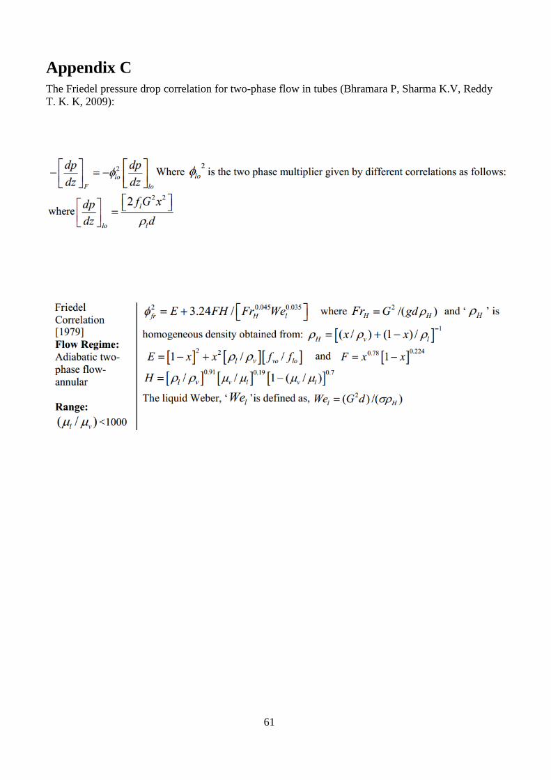
61

Appendix C

The Friedel pressure drop correlation for two-phase flow in tubes (Bhramara P, Sharma K.V, Reddy

T. K. K, 2009):

ro

be

rt e

ne

ro

th r

ob

er

t pal

Konsekvensanalys-biobränsle för eldning i en befintlig processugn i ett oljeraffinaderi

2008

chalmers univers ity of technologyse 412 96 Göteborg, SwedenPhone: + 46 - (0)31 772 10 00Web: www.chalmers.se

Konsekvensanalys-biobränsle för eldning ien befintlig processugn i ett oljeraffinaderiExamensarbete inom civilingenjörsprogrammet

robert enerothrobert pal

Institutionen för Energi och miljöAvdelningen för Värmeteknik och Maskinlärachalmers tekniska högskolaGöteborg 2008

Dynamic Modelling of Battery Cooling Systems for...

Documents

Transcript of Dynamic Modelling of Battery Cooling Systems for...