Dynamic Modeling and Simulation of an Underactuated

System

Juan Libardo Duarte Madrid1, P. A. Ospina-Henao2 and E González Querubín3

1 Facultad de Ingeniería Mecatrónica, Universidad Santo Tomás, Bucaramanga,

Colombia. 2 Departamento de Ciencias Básicas, Universidad Santo Tomás, Bucaramanga,

Colombia. 3 Facultad de Ingeniería Mecatrónica, Universidad Santo Tomás, Bucaramanga,

Colombia.

E-mail: juan.duarte03@ustabuca.edu.co, paolo.ospina@ustabuca.edu.co,

edwin.gonzalez@ustabuca.edu.co

Abstract. In this paper, is used the Lagrangian classical mechanics for modeling the dynamics

of an underactuated system, specifically a rotary inverted pendulum that will have two equations

of motion. A basic design of the system is proposed in SOLIDWORKS 3D CAD software, which

based on the material and dimensions of the model provides some physical variables necessary

for modeling. In order to verify the results obtained, a comparison the CAD model simulated in

the environment SimMechanics of MATLAB software with the mathematical model who was

consisting of Euler-Lagrange's equations implemented in Simulink MATLAB, solved with the

ODE23tb method, included in the MATLAB libraries for the solution of systems of equations of

the type and order obtained. This article also has a topological analysis of pendulum trajectories

through a phase space diagram, which allows the identification of stable and unstable regions of

the system.

1. Introduction

Nowadays, the underactuated mechanical systems [1] are generating interest among researchers of

modern control theories. This interest is that these systems have similar problems to those found in

industrial applications, such as disturbances, instabilities and nonlinear behavior in some conditions of

operation. The rotary inverted pendulum [2] is a clear example of an underactuated mechanical system;

this is a mechanism of two degrees of freedom (DOF) and two rotational joints. It consists of three main

elements: a motor, a rotational arm and a pendulum [3]. The motor shaft is connected to one end of the

rotational arm making this fully rotate on a horizontal plane; the other end of the arm has connected the

pendulum that freely rotates 360 degrees in a vertical plane. Despite being a purely academic level, this

system is helpful to study, apply and analyze different modeling strategies.

Some industrial applications [4] that present the disadvantages mentioned above, are in fields such

as robotics, robots balance, biped robots [5], robotic arms; telecommunications, satellite positioning;

transportation, Segway [6], [7], stability of ships and submarines, iBot [8], Self-balancing unicycle; and

field monitoring, drones.

For the accomplishment of this work, initially there was realized a bibliographic review of similar

projects [9], [10], [11], in order to determine the dimensions and suitable material for the later design of

the prototype in SOLIDWORKS 3D Computer Aided Engineering (CAD) software. Then, was modeled

the dynamics of the system by Lagrangian mechanics, obtaining two equations of motion; one

corresponds to the arm and other one to the pendulum. To validate the equations obtained, multiple

simulations were made in the MATLAB software in order to observe their behavior. Thus, it was

possible to verify in a graphic mode, the waveform of the angular position and velocity of the arm and

the pendulum.

A fundamental part in the stage of simulations was to import the CAD model made in

SOLIDWORKS to environment of SimMechanics [12] in MATLAB. Immediately afterwards, the

equations obtained were solved by the ODE23tb (Ordinary Differential Equations) method belonging

to MATLAB. The use of block diagram in the environment Simulink of MATLAB allowed a

representation of the equations of motion. All this had the purpose of elaborating a comparison of the

response of both the CAD model and the mathematical model obtained by the Lagrange formalism.

Finally, through the effective potential of the system the phase space diagram [13] was plotted, in

this one can see the trajectories of the pendulum and to study the critical points that correspond to the

maximum and minimum of that potential.

In Section II is defined in a broader way the rotational inverted pendulum, in addition a table is shown

that contains some variables that will be used throughout the article along with a basic design of the

system. In section III It provides a brief definition of an underactuated systems. Next, in section IV

presents the advantage of making use of Euler-Lagrange formalism. Continuing, in Section V it shows

the dynamic modeling of the proposed rotary inverted pendulum. In section VI activities are defined for

performing proposed simulations as a method of validating results. In section VII the results obtained

are shown with a respective analysis of them. Finally, section VIII contains the relevant conclusions of

the article.

2. Prototype Proposed

The pendulum is a physical object consisting of a mass joined by means of a bar to a pivot. The system

is free to move, realizing a balancing about its point of stable equilibrium; namely, in its hanging

position, in which it will be as long as there are no forces that influence its nature. In 1991 [14], there

was created the system that shows itself in the Figure 1, this device is known as Furuta's pendulum,

referring to your creator Katsuhisa Furuta. This system consists of two links only, the first one of them

is known as arm, which is an actuated element. Since this one turns freely in a horizontal plane with the

help of an electrical engine of direct current, the second one knows himself as pendulum; this one is an

underactuated element that turns freely in a vertical plane for action of the movement transmitted by the

arm. Therefore, it is a question of an underactuated system with two GDL and one control input [15].

The rotary inverted pendulum or Furuta's pendulum is of great help in the academy for the analysis

and study of strategies of classic, modern, not linear and advanced control; also, it is used with didactic

intentions for the education of the theory of control, classic mechanics and system identification.

This section presents the basic design created in SOLIDWORKS and some variables needed for

modeling.

Table 1. Variable System

Physical characteristic Symbology Units

Acceleration of gravity 𝑔 𝑚/𝑠2

Angular position of the arm 𝜃0 𝑟𝑎𝑑

Angular position of the pendulum 𝜃1 𝑟𝑎𝑑

Arm length 𝐿0 𝑚

Generalized coordinates 𝑞 𝑟𝑎𝑑

Generalized velocities �̇� 𝑟𝑎𝑑/𝑠

Kinetic Energy 𝐾 𝐽

Lagrangian ℒ 𝐽

Location of the center of mass of the pendulum 𝑙1 𝑚

Moment of inertia of the arm 𝐼0 𝑘𝑔. 𝑚2

Moment of inertia of the pendulum 𝐼1 𝑘𝑔. 𝑚2

Pendulum length 𝐿1 𝑚

Pendulum mass 𝑚1 𝑘𝑔

Potential Energy 𝑈 𝐽

Figure 1. Rotary inverted pendulum

3. Underactuated Systems

In the study of mechanisms are acquired two concepts very important such as the direct and indirect

action. The first consists of movement of elements by action of an actuator, while the second consists

of the action of motion transmitted by another interconnected element. Such movements are known as

DOF, so that mechanical systems or mechanisms can be classified depending on the number of DOF

and the number of actuators. The fully actuated mechanical systems are those having the same number

of DOF and actuators. Underactuated mechanical systems are those with fewer actuators than DOF [16].

It is important to highlight the advantages of underactuated systems, since if they do not have advantages

over fully actuated mechanical systems, it will not make sense its development. The main advantages

present in underactuated systems are energy saving and control efforts. However, these systems are

intended to perform the same functions of fully actuated systems without their disadvantages.

4. Euler-Lagrange

The dynamic equations of any mechanical system can be obtained from the known Newtonian classical

mechanics, the drawback of this formalism is the use of the variables in vector form, complicating

considerably the analysis when increasing the joints or there are rotations present in the system. In these

cases, it is favorable to employ the Lagrange equations, which have formalism of scale, facilitating the

analysis for any mechanical system.

In order to use Lagrange equations, it is necessary to follow four steps:

Calculation of kinetic energy.

Calculation of the potential energy.

Calculation of the Lagrangian.

Solve the equations.

Where the kinetic energy can be both rotationally and translational, this form of energy may be a

function of both the position and the speed 𝐾(𝑞(𝑡), �̇�(𝑡)).

The potential energy is due to conservative forces as the forces exerted by springs and gravity, this

energy is in terms of the position 𝑈(𝑞(𝑡)).

Is defined the Lagrangian as

ℒ = 𝐾 − 𝑈 (1)

Therefore, the Lagrangian in general terms is defined of the following way

ℒ(𝑞(𝑡), �̇�(𝑡)) = 𝐾(𝑞(𝑡), �̇�(𝑡)) − 𝑈(𝑞(𝑡)) (2)

Finally, are defined the Euler-Lagrange equations for a system of 𝑛 DOF as follows

𝑑

𝑑𝑡(

𝜕ℒ(𝑞, �̇�)

𝜕𝑞�̇�) −

𝜕ℒ(𝑞, �̇�)

𝜕𝑞𝑖= 𝜏𝑖

(3)

Where 𝑖 = 1, … , 𝑛, 𝜏𝑖 are the forces or pairs exerted externally in each joint, besides nonconservative

forces such as friction, resistance to movement of an object within a fluid and generally those that depend

on time or speed. It will be obtained an equal number of dynamic equations and DOF.

5. Modeling of Rotary Inverted Pendulum

Was performed the dynamic modeling of the model shown in the Figure 1. It is necessary to make an

energy analysis. Therefore, initially the kinetic energy of each link is analyzed, so it can be identified

which kinetic energies (rotational and translational) were present in each link.

5.1. Kinetic Energy

The kinetic energy of the system consist of a translational and rotational component for the pendulum

and rotational component for the arm

𝐾 =1

2𝑚𝑣2 +

1

2𝐼𝜔2

(4)

Where 𝑚 is the mass of the body, 𝑣 the linear velocity, 𝐼 the moment of inertia, 𝜔 the angular velocity

and 𝐾 the kinetic energy. In this case, there are two bodies, the arm and the pendulum. The kinetic

energy of the arm is

𝐾0 =1

2𝐼0�̇�0

2

(5)

The kinetic energy of the pendulum is

𝐾1 =1

2𝑚1𝑣1

2 +1

2𝐼1�̇�1

2

(6)

The total energy of the system is

𝐾𝑇 =1

2𝐼0�̇�0

2+

1

2𝑚1𝑣1

2 +1

2𝐼1�̇�1

2

(7)

5.2. Potential Energy

This system only store gravitational potential energy in the pendulum

𝑈 = 𝑚𝑔ℎ (8)

The arm has in its nature a rotational movement in a horizontal plane, therefore it does not have height

change in its center of mass, providing equal 0 component in equation (8) resulting in a potential energy

zero .

The potential energy of the pendulum is

𝑈1 = 𝑚1𝑔𝑙1(cos 𝜃1 − 1) (9)

Where 𝑔 represents the value of gravity. The total potential energy of the system is (9)

𝑈𝑇 = 𝑚1𝑔𝑙1(cos 𝜃1 − 1) (10)

5.3. Position of the pendulum

Because the pendulum is a rigid body, the required position is the its center of mass

Figure 2. Projection arm and pendulum in the 𝑥𝑦 plane

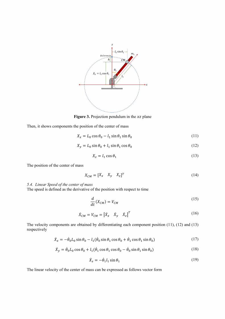
Figure 3. Projection pendulum in the 𝑥𝑧 plane

Then, it shows components the position of the center of mass

𝑋𝑥 = 𝐿0 cos 𝜃0 − 𝑙1 sin 𝜃1 sin 𝜃0 (11)

𝑋𝑦 = 𝐿0 sin 𝜃0 + 𝑙1 sin 𝜃1 cos 𝜃0 (12)

𝑋𝑧 = 𝑙1 cos 𝜃1 (13)

The position of the center of mass

𝑋𝐶𝑀 = [𝑋𝑥 𝑋𝑦 𝑋𝑧]𝑇 (14)

5.4. Linear Speed of the center of mass

The speed is defined as the derivative of the position with respect to time

𝑑

𝑑𝑡(𝑋𝐶𝑀) = 𝑉𝐶𝑀

(15)

�̇�𝐶𝑀 = 𝑉𝐶𝑀 = [�̇�𝑥 �̇�𝑦 �̇�𝑧]𝑇

(16)

The velocity components are obtained by differentiating each component position (11), (12) and (13)

respectively

�̇�𝑥 = −�̇�0𝐿0 sin 𝜃0 − 𝑙1(�̇�0 sin 𝜃1 cos 𝜃0 + �̇�1 cos 𝜃1 sin 𝜃0) (17)

�̇�𝑦 = �̇�0𝐿0 cos 𝜃0 + 𝑙1(�̇�1 cos 𝜃1 cos 𝜃0 − �̇�0 sin 𝜃1 sin 𝜃0) (18)

�̇�𝑧 = −�̇�1𝑙1 sin 𝜃1 (19)

The linear velocity of the center of mass can be expressed as follows vector form

𝑉𝐶𝑀2 = [�̇�𝑥 �̇�𝑦 �̇�𝑧] [

�̇�𝑥

�̇�𝑦

�̇�𝑧

] = �̇�𝑥2

+ �̇�𝑦2

+ �̇�𝑧2

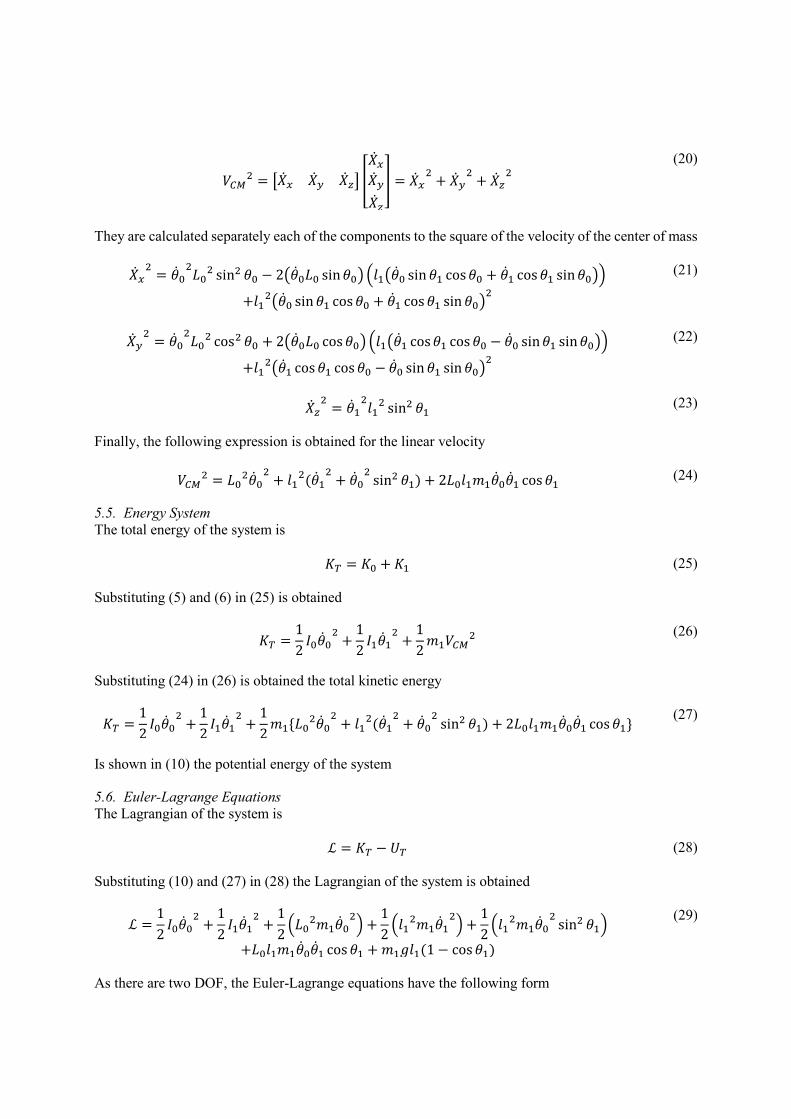
(20)

They are calculated separately each of the components to the square of the velocity of the center of mass

�̇�𝑥2

= �̇�02

𝐿02 sin2 𝜃0 − 2(�̇�0𝐿0 sin 𝜃0) (𝑙1(�̇�0 sin 𝜃1 cos 𝜃0 + �̇�1 cos 𝜃1 sin 𝜃0))

+𝑙12(�̇�0 sin 𝜃1 cos 𝜃0 + �̇�1 cos 𝜃1 sin 𝜃0)

2

(21)

�̇�𝑦2

= �̇�02

𝐿02 cos2 𝜃0 + 2(�̇�0𝐿0 cos 𝜃0) (𝑙1(�̇�1 cos 𝜃1 cos 𝜃0 − �̇�0 sin 𝜃1 sin 𝜃0))

+𝑙12(�̇�1 cos 𝜃1 cos 𝜃0 − �̇�0 sin 𝜃1 sin 𝜃0)

2

(22)

�̇�𝑧2

= �̇�12

𝑙12 sin2 𝜃1 (23)

Finally, the following expression is obtained for the linear velocity

𝑉𝐶𝑀2 = 𝐿0

2�̇�02

+ 𝑙12(�̇�1

2+ �̇�0

2sin2 𝜃1) + 2𝐿0𝑙1𝑚1�̇�0�̇�1 cos 𝜃1 (24)

5.5. Energy System

The total energy of the system is

𝐾𝑇 = 𝐾0 + 𝐾1 (25)

Substituting (5) and (6) in (25) is obtained

𝐾𝑇 =1

2𝐼0�̇�0

2+

1

2𝐼1�̇�1

2+

1

2𝑚1𝑉𝐶𝑀

2 (26)

Substituting (24) in (26) is obtained the total kinetic energy

𝐾𝑇 =1

2𝐼0�̇�0

2+

1

2𝐼1�̇�1

2+

1

2𝑚1{𝐿0

2�̇�02

+ 𝑙12(�̇�1

2+ �̇�0

2sin2 𝜃1) + 2𝐿0𝑙1𝑚1�̇�0�̇�1 cos 𝜃1}

(27)

Is shown in (10) the potential energy of the system

5.6. Euler-Lagrange Equations

The Lagrangian of the system is

ℒ = 𝐾𝑇 − 𝑈𝑇 (28)

Substituting (10) and (27) in (28) the Lagrangian of the system is obtained

ℒ =1

2𝐼0�̇�0

2+

1

2𝐼1�̇�1

2+

1

2(𝐿0

2𝑚1�̇�02

) +1

2(𝑙1

2𝑚1�̇�12

) +1

2(𝑙1

2𝑚1�̇�02

sin2 𝜃1)

+𝐿0𝑙1𝑚1�̇�0�̇�1 cos 𝜃1 + 𝑚1𝑔𝑙1(1 − cos 𝜃1)

(29)

As there are two DOF, the Euler-Lagrange equations have the following form

𝑑

𝑑𝑡(

𝜕ℒ

𝜕�̇�0

) −𝜕ℒ

𝜕𝜃0= 𝜏

(30)

𝑑

𝑑𝑡(

𝜕ℒ

𝜕�̇�1

) −𝜕ℒ

𝜕𝜃1= 0

(31)

Where 𝜏 is the torque of motor, solving (30) and (31) we obtain the equations of motion which are given

by

𝐼0�̈�0 + 𝐿02𝑚1�̈�0 +

{𝑙12𝑚1 (�̈�0 sin2 𝜃1 + 2�̇�0�̇�1 sin 𝜃1 cos 𝜃1)} + {𝐿0𝑙1𝑚1( �̈�1 cos 𝜃1 − �̇�1

2sin 𝜃1)} = 𝜏

(32)

𝐼1�̈�1 + 𝑙12𝑚1�̈�1 + 𝐿0𝑙1𝑚1�̈�0 cos 𝜃1 − 𝑙1

2𝑚1�̇�02

sin 𝜃1 cos 𝜃1 − 𝑚1𝑔𝑙1 sin 𝜃1 = 0 (33)

Where (32) is the equation of motion of the arm and (33) of the pendulum.

6. Simulation

Although the Euler-Lagrange formalism ensures a high degree of approximation of the mathematical

models, is essential do comparisons to validate these results. Are followed the next steps for verification

of modeling:

1) Represent the system equations in the state space.

2) Define an experiment with initial conditions, natural interactions and external forces.

3) Import the CAD model of SOLIDWORKS in SimMechanics-MATLAB.

4) Add the necessary blocks to obtain the desired graphic model and applying external forces.

5) Simulating experiment.

6) Export the results of SimMechanics to Workspace MATLAB.

7) Implement a block diagram Simulink-MATLAB to solve the equations.

8) Export the solutions to the equations to Workspace MATLAB.

9) Graphing and overlay solutions.

As can be seen in the steps above, the simulation of the model was divided in two stages: first, simulate

the CAD model initially designed and the second implement the equations obtained.

7. Results

Then, it presents each of the steps mentioned in the previous section.

1) Starting from [17]

𝑀(𝑞)�̈� + 𝐶(𝑞, �̇�)�̇� + 𝐺(𝑞) = 𝜏 (34)

Therefore, the equation (34) is the dynamic equation for mechanical systems of n DOF. Where, 𝑀 is the

matrix of inertia, 𝐶 is the centrifugal and Coriolis matrix, 𝐺 the vector of gravity and 𝜏 external forces.

Taking the equations of motion (32) and (33) and replacing in (34) is obtained a matrix representation

[𝐼𝑜 + 𝑚1𝐿0

2 + 𝑙12𝑚1 sin2 𝜃1 𝐿0𝑙1𝑚1 cos 𝜃1

𝐿0𝑙1𝑚1 cos 𝜃1 𝐼1 + 𝑚1𝑙12 ] [

�̈�0

�̈�1

]

+ [2𝑙1

2𝑚1 sin 𝜃1 cos 𝜃1 �̇�1 −𝐿0𝑙1𝑚1 sin 𝜃1 �̇�1

−𝑙12𝑚1 sin 𝜃1 cos 𝜃1 �̇�0 0

] [�̇�0

�̇�1

] + [0

−𝑔𝑙1𝑚1 sin 𝜃1] = [

𝜏0

]

(35)

The matrix 𝑀(𝑞) is important for the dynamic modeling and for the design of controllers. This matrix

has a great relationship with the kinetic energy, also the inertia matrix is a symmetric, positive and

square matrix of 𝑛 × 𝑛, whose elements depend only on the generalized coordinates.

Centrifugal and Coriolis matrix 𝐶(𝑞, �̇�) it is important in the study of stability in control systems,

mechanical systems, among others. This matrix is square of 𝑛 × 𝑛 and has dependence in its elements

of the generalized coordinates and velocities.

The gravity vector 𝐺(𝑞) it is present in mechanical systems without counterweights or springs, in

turn is in systems with displacement off the horizontal plane. This vector is of 𝑛 × 1 and has only

reliance on joint positions.

2) It defined that the system would have the initial conditions shown in Figure 5, in addition to being

subject to effects of gravity and to a torque step 0.2 seconds in the end of the arm that connects to the

motor shaft. Finally, a simulation interval 5 seconds was established.

3) Was imported the CAD model in SimMechanics with the following code line:

mech_import(‘CADModel_Pendulum.xml’). The initial position of the system is Figure 5 a).

4) It was necessary add a few block the diagram SimMechanics, since the CAD model is only under

the effect of gravity and not have some kind of movement, it blocks provide the step of torque arm

included to start rotating, besides adding blocks to the sensing of angular displacement and velocities in

an interval of 5 second of test.

Figure 4. Final block diagram in SimMechanics

The Figure 4 shows the block diagram implemented for the simulation of the CAD model. The block

named Subsystem1 contains the majority of the blocks generated of the CAD model by SimMechanics,

such blocks are not necessary for the simulation; others blocks generated by SimMechanics are

Revolute2, EjeMotor-1, Weld1, Brazo-1, Revolute1, Brazo2-1, Weld3, AcoplePendulo-1, Weld2 and

Pendulo-1. The most important elements for the simulation are the blocks Revolute; Revolute2 is the

joint of the arm, theoretically it is there where there would be connected the electrical engine, which in

this case is simulated by a Joint Actuator configured as a force generator. The block MATLAB Function

contains a small code that generates a torque of 0.5 Nm in an interval of 0.2 seconds; to simulate the

motor encoder the Joint Sensor block is connected, of which there is obtained the speed of arm it �̇�0

(Figure 11), and with an of integration block (Integrator0) the position of same one it 𝜃0 (Figure 9). For

the case of the Revolute1 there is a bit different the way of obtaining the variables of interest, this

difference owes to the CAD design in SOLIDWORKS, since both the arm and the pendulum have design

and couplings different. In Revolute1 there connects a block called Joint Initial Condition, in which it is

possible to change the initial position of the pendulum, in this link we will not have any engine, since

as mentioned in the section II it is a question of the underactuated element. On the other hand, it is

necessary to simulate an encoder to know the position of the pendulum in any instant of time, for this

implemented the block Body Sensor1, which is used to measure the position of the center of mass of the

pendulum. So that, there is obtained initially the angular speed of the pendulum it �̇�1 (Figure 10) and of

equal way that with the arm, by means of an integrator (Integrator1) obtains the angular position it 𝜃1

(Figure 8).

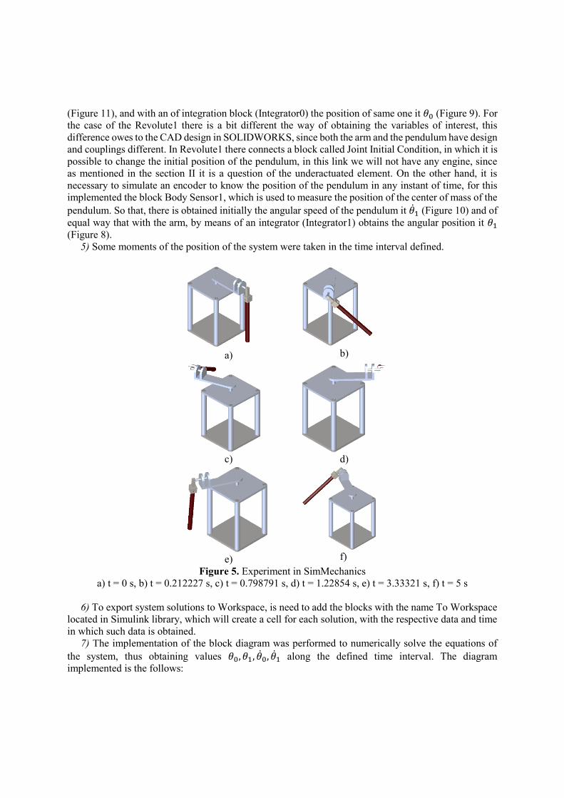
5) Some moments of the position of the system were taken in the time interval defined.

a)

b)

c)

d)

e)

f)

Figure 5. Experiment in SimMechanics

a) t = 0 s, b) t = 0.212227 s, c) t = 0.798791 s, d) t = 1.22854 s, e) t = 3.33321 s, f) t = 5 s

6) To export system solutions to Workspace, is need to add the blocks with the name To Workspace

located in Simulink library, which will create a cell for each solution, with the respective data and time

in which such data is obtained.

7) The implementation of the block diagram was performed to numerically solve the equations of

the system, thus obtaining values 𝜃0, 𝜃1, �̇�0, �̇�1 along the defined time interval. The diagram

implemented is the follows:

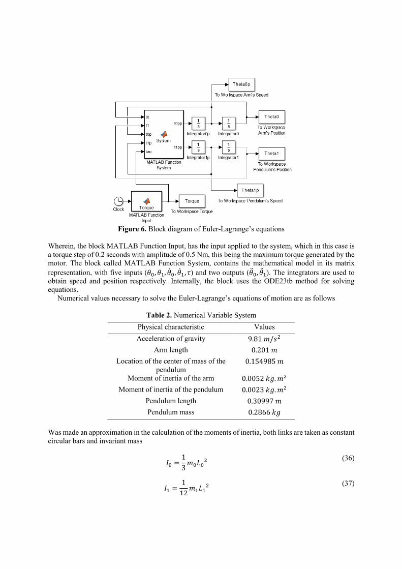
Figure 6. Block diagram of Euler-Lagrange’s equations

Wherein, the block MATLAB Function Input, has the input applied to the system, which in this case is

a torque step of 0.2 seconds with amplitude of 0.5 Nm, this being the maximum torque generated by the

motor. The block called MATLAB Function System, contains the mathematical model in its matrix

representation, with five inputs (𝜃0, 𝜃1, �̇�0, �̇�1, 𝜏) and two outputs (�̈�0, �̈�1). The integrators are used to

obtain speed and position respectively. Internally, the block uses the ODE23tb method for solving

equations.

Numerical values necessary to solve the Euler-Lagrange’s equations of motion are as follows

Table 2. Numerical Variable System

Physical characteristic Values

Acceleration of gravity 9.81 𝑚/𝑠2

Arm length 0.201 𝑚

Location of the center of mass of the

pendulum 0.154985 𝑚

Moment of inertia of the arm 0.0052 𝑘𝑔. 𝑚2

Moment of inertia of the pendulum 0.0023 𝑘𝑔. 𝑚2

Pendulum length 0.30997 𝑚

Pendulum mass 0.2866 𝑘𝑔

Was made an approximation in the calculation of the moments of inertia, both links are taken as constant

circular bars and invariant mass

𝐼0 =1

3𝑚0𝐿0

2 (36)

𝐼1 =1

12𝑚1𝐿1

2 (37)

Where (36) is the moment of inertia of the arm; measured from the end connected to the motor shaft to

the opposite end. While (37) is the pendulum moment of inertia; measured pendulum from the center of

mass.

8) The way to export the data to Workspace of block diagram above is performed with the same

aggregate block in step 6).

9) Taking the exported data in points 6) and 8) the following graphs were made.

Figure 7. Step torque

Figure 8. Angular position of pendulum with

CAD model

Figure 9. Angular position of arm with CAD

model

Figure 10. Angular velocity of pendulum with

CAD model

Figure 11. Angular velocity of arm with CAD

model

Figure 12. Angular position of pendulum with

Euler-Lagrange’s equations

Figure 13. Angular position of arm with

Euler-Lagrange’s equations

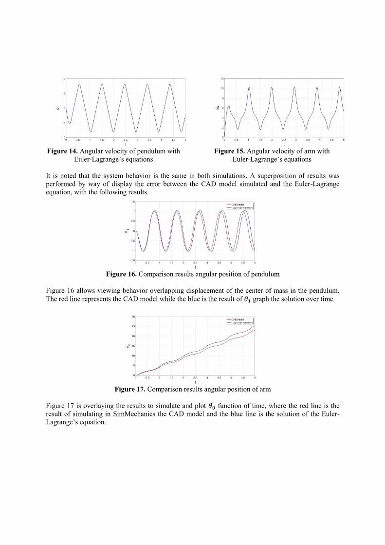
Figure 14. Angular velocity of pendulum with

Euler-Lagrange’s equations

Figure 15. Angular velocity of arm with

Euler-Lagrange’s equations

It is noted that the system behavior is the same in both simulations. A superposition of results was

performed by way of display the error between the CAD model simulated and the Euler-Lagrange

equation, with the following results.

Figure 16. Comparison results angular position of pendulum

Figure 16 allows viewing behavior overlapping displacement of the center of mass in the pendulum.

The red line represents the CAD model while the blue is the result of 𝜃1 graph the solution over time.

Figure 17. Comparison results angular position of arm

Figure 17 is overlaying the results to simulate and plot 𝜃0 function of time, where the red line is the

result of simulating in SimMechanics the CAD model and the blue line is the solution of the Euler-

Lagrange’s equation.

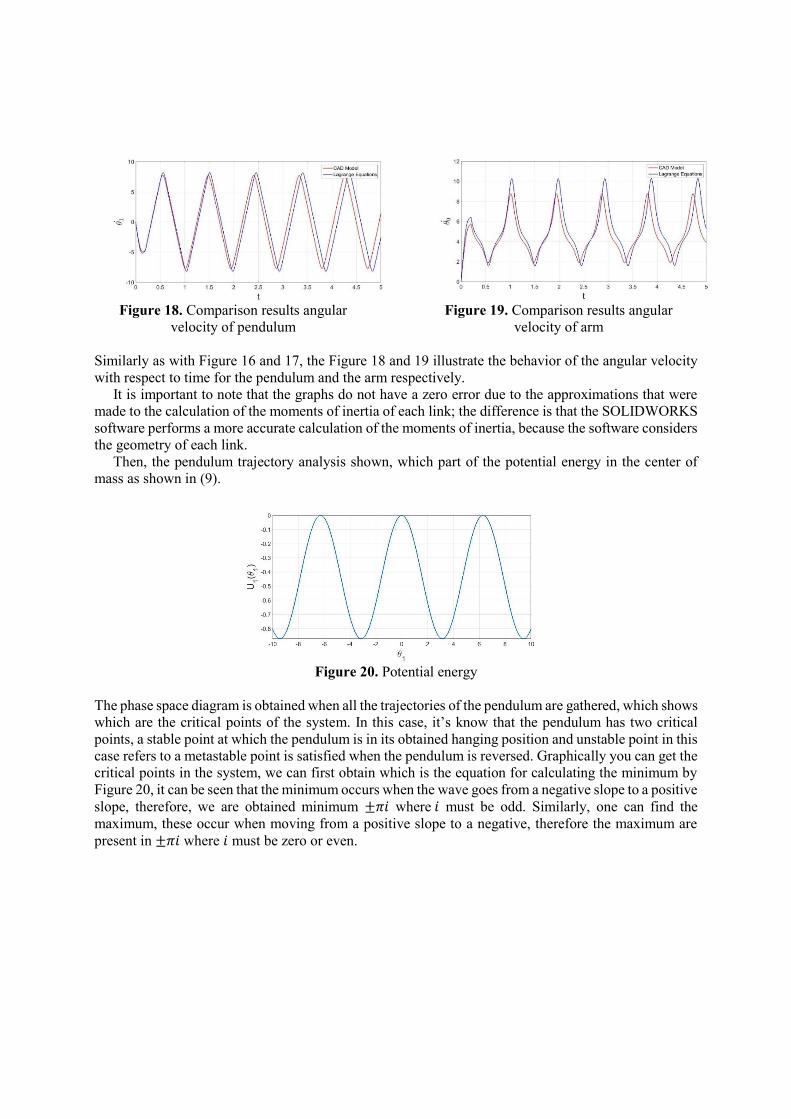
Figure 18. Comparison results angular

velocity of pendulum

Figure 19. Comparison results angular

velocity of arm

Similarly as with Figure 16 and 17, the Figure 18 and 19 illustrate the behavior of the angular velocity

with respect to time for the pendulum and the arm respectively.

It is important to note that the graphs do not have a zero error due to the approximations that were

made to the calculation of the moments of inertia of each link; the difference is that the SOLIDWORKS

software performs a more accurate calculation of the moments of inertia, because the software considers

the geometry of each link.

Then, the pendulum trajectory analysis shown, which part of the potential energy in the center of

mass as shown in (9).

Figure 20. Potential energy

The phase space diagram is obtained when all the trajectories of the pendulum are gathered, which shows

which are the critical points of the system. In this case, it’s know that the pendulum has two critical

points, a stable point at which the pendulum is in its obtained hanging position and unstable point in this

case refers to a metastable point is satisfied when the pendulum is reversed. Graphically you can get the

critical points in the system, we can first obtain which is the equation for calculating the minimum by

Figure 20, it can be seen that the minimum occurs when the wave goes from a negative slope to a positive

slope, therefore, we are obtained minimum ±𝜋𝑖 where 𝑖 must be odd. Similarly, one can find the

maximum, these occur when moving from a positive slope to a negative, therefore the maximum are

present in ±𝜋𝑖 where 𝑖 must be zero or even.

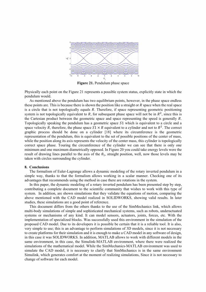
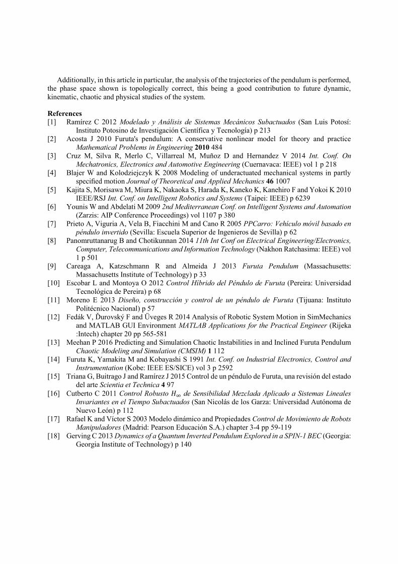
Figure 21. Pendulum phase space

Physically each point on the Figure 21 represents a possible system status, explicitly state in which the

pendulum would.

As mentioned above the pendulum has two equilibrium points, however, in the phase space endless

these points are. This is because there is shown the position like a straight or 𝑅 space when the real space

is a circle that is not topologically equals 𝑅. Therefore, if space representing geometric positioning

system is not topologically equivalent to 𝑅, for subsequent phase space will not be in 𝑅2, since this is

the Cartesian product between the geometric space and space representing the speed is generally 𝑅.

Topologically speaking the pendulum has a geometric space 𝑆1 which is equivalent to a circle and a

space velocity 𝑅, therefore, the phase space 𝑆1 × 𝑅 equivalent to a cylinder and not to 𝑅2. The correct

graphic process should be done on a cylinder [18] where its circumference is the geometric

representation of the pendulum, this is equivalent to the set of possible positions of the center of mass,

while the position along its axis represents the velocity of the center mass, this cylinder is topologically

correct space phase. Touring the circumference of the cylinder we can see that there is only one

minimum and one maximum diametrically opposed. In Figure 20 you could take energy levels were the

result of drawing lines parallel to the axis of the 𝜃1, straight position, well, now those levels may be

taken with circles surrounding the cylinder.

8. Conclusions

The formalism of Euler-Lagrange allows a dynamic modeling of the rotary inverted pendulum in a

simple way, thanks to that the formalism allows working in a scalar manner. Checking one of its

advantages that recommends using the method in case there are rotations in the system.

In this paper, the dynamic modeling of a rotary inverted pendulum has been presented step by step,

contributing a complete document to the scientific community that wishes to work with this type of

system. In addition, are shown simulations that they validate the equations of motion, comparing the

above mentioned with the CAD model realized in SOLIDWORKS, showing valid results. In later

studies, these simulations are a good point of reference.

This document differs from the others thanks to the use of the SimMechanics link, which allows

multi-body simulations of simple and sophisticated mechanical systems, such as robots, underactuated

systems or mechanisms of any kind. It can model sensors, actuators, joints, forces, etc. With the

implementation of specialized blocks. Was successfully used this environment in the simulation of the

proposed CAD model. Due to its developers it is possible be certain that it is a reliable tool. It is also,

very simple to use; this is an advantage to perform simulations of 3D models, since it is not necessary

to create platforms for their simulation and it is enough to make a CAD model in any software of design,

in this case it was SOLIDWORKS. In addition, MATLAB allows to work with different models in the

same environment, in this case, the Simulink-MATLAB environment, where there were realized the

simulations of the mathematical model. While the SimMechanics-MATLAB environment was used to

simulate the CAD model, it is necessary to clarify that SimMechanics is in the same environment

Simulink, which generates comfort at the moment of realizing simulations, Since it is not necessary to

change of software for each model.

Additionally, in this article in particular, the analysis of the trajectories of the pendulum is performed,

the phase space shown is topologically correct, this being a good contribution to future dynamic,

kinematic, chaotic and physical studies of the system.

References

[1] Ramírez C 2012 Modelado y Análisis de Sistemas Mecánicos Subactuados (San Luis Potosí:

Instituto Potosino de Investigación Científica y Tecnología) p 213

[2] Acosta J 2010 Furuta's pendulum: A conservative nonlinear model for theory and practice

Mathematical Problems in Engineering 2010 484

[3] Cruz M, Silva R, Merlo C, Villarreal M, Muñoz D and Hernandez V 2014 Int. Conf. On

Mechatronics, Electronics and Automotive Engineering (Cuernavaca: IEEE) vol 1 p 218

[4] Blajer W and Kolodziejczyk K 2008 Modeling of underactuated mechanical systems in partly

specified motion Journal of Theoretical and Applied Mechanics 46 1007

[5] Kajita S, Morisawa M, Miura K, Nakaoka S, Harada K, Kaneko K, Kanehiro F and Yokoi K 2010

IEEE/RSJ Int. Conf. on Intelligent Robotics and Systems (Taipei: IEEE) p 6239

[6] Younis W and Abdelati M 2009 2nd Mediterranean Conf. on Intelligent Systems and Automation

(Zarzis: AIP Conference Proceedings) vol 1107 p 380

[7] Prieto A, Viguria A, Vela B, Fiacchini M and Cano R 2005 PPCarro: Vehículo móvil basado en

péndulo invertido (Sevilla: Escuela Superior de Ingenieros de Sevilla) p 62

[8] Panomruttanarug B and Chotikunnan 2014 11th Int Conf on Electrical Engineering/Electronics,

Computer, Telecommunications and Information Technology (Nakhon Ratchasima: IEEE) vol

1 p 501

[9] Careaga A, Katzschmann R and Almeida J 2013 Furuta Pendulum (Massachusetts:

Massachusetts Institute of Technology) p 33

[10] Escobar L and Montoya O 2012 Control Híbrido del Péndulo de Furuta (Pereira: Universidad

Tecnológica de Pereira) p 68

[11] Moreno E 2013 Diseño, construcción y control de un péndulo de Furuta (Tijuana: Instituto

Politécnico Nacional) p 57

[12] Fedák V, Ďurovský F and Üveges R 2014 Analysis of Robotic System Motion in SimMechanics

and MATLAB GUI Environment MATLAB Applications for the Practical Engineer (Rijeka

:Intech) chapter 20 pp 565-581

[13] Meehan P 2016 Predicting and Simulation Chaotic Instabilities in and Inclined Furuta Pendulum

Chaotic Modeling and Simulation (CMSIM) 1 112

[14] Furuta K, Yamakita M and Kobayashi S 1991 Int. Conf. on Industrial Electronics, Control and

Instrumentation (Kobe: IEEE ES/SICE) vol 3 p 2592

[15] Triana G, Buitrago J and Ramírez J 2015 Control de un péndulo de Furuta, una revisión del estado

del arte Scientia et Technica 4 97

[16] Cutberto C 2011 Control Robusto 𝐻∞ de Sensibilidad Mezclada Aplicado a Sistemas Lineales

Invariantes en el Tiempo Subactuados (San Nicolás de los Garza: Universidad Autónoma de

Nuevo León) p 112

[17] Rafael K and Víctor S 2003 Modelo dinámico and Propiedades Control de Movimiento de Robots

Manipuladores (Madrid: Pearson Educación S.A.) chapter 3-4 pp 59-119

[18] Gerving C 2013 Dynamics of a Quantum Inverted Pendulum Explored in a SPIN-1 BEC (Georgia:

Georgia Institute of Technology) p 140