TI 2009-041/4 Tinbergen Institute Discussion Paper

Dynamic Factor Models with Smooth Loadings for Analyzing the Term Structure of Interest Rates

Borus Jungbackera

Siem Jan Koopmana,c Michel van der Welb,c,d,e

a VU University Amsterdam; b Erasmus University Rotterdam; c Tinbergen Institute; d ERIM; e CREATES, Aarhus.

brought to you by COREView metadata, citation and similar papers at core.ac.uk

provided by DSpace at VU

Tinbergen Institute The Tinbergen Institute is the institute for economic research of the Erasmus Universiteit Rotterdam, Universiteit van Amsterdam, and Vrije Universiteit Amsterdam. Tinbergen Institute Amsterdam Roetersstraat 31 1018 WB Amsterdam The Netherlands Tel.: +31(0)20 551 3500 Fax: +31(0)20 551 3555 Tinbergen Institute Rotterdam Burg. Oudlaan 50 3062 PA Rotterdam The Netherlands Tel.: +31(0)10 408 8900 Fax: +31(0)10 408 9031 Most TI discussion papers can be downloaded at http://www.tinbergen.nl.

Smooth Dynamic Factor Analysis with an Application

to the U.S. Term Structure of Interest Rates

Borus Jungbacker (a) Siem Jan Koopman(a,b) Michel van der Wel (b,c)

(a) Department of Econometrics, VU University Amsterdam

(b) Tinbergen Institute

(c) Erasmus School of Economics, ERIM Rotterdam and CREATES, Aarhus

September 14, 2010

Some keywords : Fama-Bliss data set; Kalman filter; Maximum likelihood; Yield curve.

JEL classification: C32, C51, E43.

Acknowledgements: We would like to thank Francis X. Diebold and Dick van Dijk for

their comments on an earlier version of this paper. Furthermore, we have benefited from

the comments by conference participants of the 10th Econometric Society World Congress

in Shanghai (August 2010), the 16th International Conference on Panel Data at Univer-

sity of Amsterdam (July 2010), the International Symposium on Econometric Theory and

Applications at Singapore Management University (April 2010), the 2nd Amsterdam-Bonn

workshop in Econometrics at Tinbergen Institute (May 2010), the Yield Curve Modeling

workshop at Econometric Institute of the Erasmus University Rotterdam (June 2010), the

Econometric Society European Meetings (ESEM) in Barcelona (August 2009) and the 3rd

International Conference on Computational and Financial Econometrics in Limassol, Cyprus

(October 2009), and from participants of seminars at CREATES of Aarhus University (April

2009) and Federal Reserve Board in Washington DC (March 2010). Further details of our

estimation procedure and its results reported in this paper are available from the authors

upon request. Possible remaining errors are our own. Michel van der Wel acknowledges the

support from CREATES, funded by the Danish National Research Foundation.

Address of correspondence: S.J. Koopman, Department of Econometrics, VU University

Amsterdam, De Boelelaan 1105, NL-1081 HV Amsterdam, The Netherlands.

Emails : bjungbacker@feweb.vu.nl s.j.koopman@feweb.vu.nl vanderwel@ese.eur.nl

0

Smooth Dynamic Factor Analysis with an Application

to the U.S. Term Structure of Interest Rates

Borus Jungbacker, Siem Jan Koopman and Michel van der Wel

Abstract

We consider the dynamic factor model and show how smoothness restrictions can be

imposed on the factor loadings. Cubic spline functions are used to introduce smooth-

ness in factor loadings. We develop statistical procedures based on Wald, Lagrange

multiplier and likelihood ratio tests for this purpose. A Monte Carlo study is presented

to show that our procedures are successful in identifying smooth loading structures

from small sample panels. We illustrate the methodology by analyzing the U.S. term

structure of interest rates. An empirical study is carried out using a monthly time

series panel of unsmoothed Fama-Bliss zero yields for treasuries of different maturities

between 1970 and 2009. Dynamic factor models with and without smooth loadings are

compared with dynamic models based on Nelson-Siegel and cubic spline yield curves.

All models can be regarded as special cases of the dynamic factor model. We carry

out statistical hypothesis tests and compare information criteria to verify whether the

restrictions imposed by the models are supported by the data. Out-of-sample forecast

evidence is also given. Our main conclusion is that smoothness restrictions on loadings

of the dynamic factor model for the term structure can be supported by our panel of

U.S. interest rates and can lead to more accurate forecasts.

1

1 Introduction

The general dynamic factor model increasingly plays a major role in econometrics. Early

contributions to the literature on dynamic factor models can be found in Sargent and Sims

(1977), Geweke (1977), Engle and Watson (1981), Watson and Engle (1983), Connor and

Korajczyk (1993) and Gregory, Head, and Raynauld (1997). Most of these papers consider

time series panels with limited panel dimensions. The increasing availability of high dimen-

sional data sets has intensified the quest for computationally efficient estimation methods.

The strand of literature headed by Forni, Hallin, Lippi, and Reichlin (2000), Stock and

Watson (2002) and Bai (2003) led to a renewed interest in dynamic factor analysis. These

methods are typically applied to high dimensional panels of time series. Exact maximum

likelihood methods such as proposed in Watson and Engle (1983) have traditionally been

dismissed as computationally too intensive for such high dimensional panels. An exception

is the study by Quah and Sargent (1993) who consider a moderately sized panel of economic

time series in their study. Jungbacker and Koopman (2008) however present new results

that facilitate application of exact maximum likelihood methods for very high dimensional

panels. Examples of recent papers employing likelihood-based methods for the analysis of

dynamic factor models are Doz, Giannone, and Reichlin (2006) and Reis and Watson (2010).

In this paper we develop an econometric likelihood-based framework for the introduction

of smoothness in the factor loadings of a dynamic factor model. The smoothness conditions

on the loadings are first introduced via spline functions that depend on knot coefficients, see

Poirier (1976). We develop next statistical procedures based on Wald, Lagrange multiplier

and likelihood ratio tests for finding a suitable set of restrictions. General to specific and

specific to general approaches are discussed and compared with each other. Monte Carlo

evidence is provided to show that smoothness conditions can be detected accurately while

some preference is given to the specific to general approach of determining the smoothness

in factor loadings. The idea of imposing smoothness in loadings has earlier been considered

by Fengler, Haerdle, and Schmidt (2002) in an application of analyzing volatility in financial

markets. Their approach is recently developed further using semiparametrics methods by

Park, Mammen, Haerdle, and Borak (2009). Here we develop a full maximum likelihood

procedure for imposing smoothness in the factor structure.

There are several motivations to impose smoothness on the factor loadings in a dynamic

factor model. The economic motivation of smooth loadings is to establish an interpretation

for the factors. When the factor loadings are related to particular characteristics of the

corresponding variables in the panel, we can impose this relationship by specifying a smooth

flexible function for the factor loading coefficients. A smooth pattern in a column of the

2

loading matrix can lead to an interpretable factor that is associated with this column. In

our empirical study for a panel of interest rates, we impose smoothness on the loadings

through a spline function that depends on time to maturity. The common interpretation of

the factors as level, slope and curvature of the yield curve can be established. Also in other

cases a smooth relationship between the underlying factors and observations may exist. Our

model could therefore be applied in other applications, including modelling volatility and

analyzing electricity prices. The econometric motivation of smooth loadings is the aim for a

parsimonious model specification where individual loading coefficients are interpolated by a

flexible function that depends on a small number of coefficients. The precision of parameter

estimates is generally increased by considering more parsimonious models. Furthermore,

smoothness in factor loadings may also lead to models that are more robust to aberrant

observations. It is also often argued that forecasts based on a model with a small set

of parameters can be expected to be more precise than those based on a less parsimonious

model; see the discussion in Clements and Hendry (1998). We develop a flexible new method

for introducing smoothness in the loadings for each dynamic factor in the model.

To empirically investigate whether our method of imposing smoothness restrictions on

factor loadings is effective, we analyze a panel of U.S. interest rate series for different times to

maturity. In the modelling of interest rates it is common to assume that the term structure of

different maturities (or yield curve) is driven by a small set of unobserved stochastic factors.

In this paper we consider the general dynamic factor model for analyzing the term structure

of interest rates. The yield curve tends to be a smooth function of time to maturity. It

is therefore reasonable to assume that the factor loadings are smooth functions of time to

maturity as well. The primary aim of our paper is to find empirical evidence to support

the assumption of smooth factor loadings. For this purpose, we consider the dynamic factor

model with and without smoothness, together with two alternative model specifications.

The alternative model specifications are the dynamic Nelson-Siegel model and the func-

tional signal plus noise model. The first model for the term structure is based on the seminal

paper of Nelson and Siegel (1987) in which the yield curve is approximated by a weighted

sum of three smooth functions. The form of these three functions depends on a single param-

eter. Diebold and Li (2006) use the Nelson-Siegel framework to develop a two-step procedure

for the forecasting of future yields. They show that forecasts obtained from this procedure

are competitive with forecasts obtained from other standard prediction methods. Diebold,

Rudebusch, and Aruoba (2006) integrate the two-step approach into a single dynamic factor

model by specifying the Nelson-Siegel weights as an unobserved vector autoregressive pro-

cess. A generalization of their state space approach is considered by Koopman, Mallee, and

Van der Wel (2010), who allow the parameter governing the shape of the Nelson-Siegel func-

3

tions to be time-varying and who allow for the inclusion of conditional heteroskedasticity for

the innovations in the model. Due to its popularity amongst practitioners, central bankers

and academics, the Nelson-Siegel model serves as our benchmark term structure model. The

dynamic Nelson-Siegel model can also be regarded as a special case of the dynamic factor

model and we compare it with our smooth dynamic factor model in the empirical study.

The second model is recently discussed by Bowsher and Meeks (2008) and represents the

term structure as a cubic spline function that is observed with measurement noise. The pa-

rameters controlling the shape of the spline are time-varying and modelled as a cointegrated

vector autoregressive process with different numbers of lags. We consider a basic version of

this model and also compare it with the other models in our empirical study that focuses

both on in-sample and out-of-sample results. Related work on factor structures in the term

structure of interest rates has appeared recently. For example, Duffee (2009) studies restric-

tions on general factor models of the term structure imposed by arbitrage relationships with

a focus on forecasting performance while Lengwiler and Lenz (2010) develop a factor model

for the yield curve in which the innovations of the factors are mutually orthogonal. This

paper considers smoothness in dynamic factor models generally. While our empirical study

concerns the yield curve, our framework can be applied in different circumstances as well.

The empirical study is considering a newly constructed monthly time series panel of

unsmoothed Fama-Bliss zero yields for U.S. treasuries of different maturities between 1970

and 2009. The data set is used to empirically validate the aforementioned models. Our

main empirical finding is that the dynamic factor model without restrictions on the factor

loadings is able to fit the yield curve very accurately. In other words, the standard errors

of the estimated factor loadings are small overall. This finding implies that for imposing

smoothing restrictions on the factor loadings, the smoothing functions must be sufficiently

flexible to closely match the smooth loadings with the unrestricted loadings. Although

likelihood ratio tests reject all considered restricted dynamic factor models, the likelihood of

our smooth dynamic factor model is closest to the likelihood of the unrestricted model while

the Schwarz information criterion indicates that it is the preferred dynamic factor model. We

also investigate the forecasting ability of the considered models. Our smooth dynamic factor

model produces forecasts that are more accurate than those for the unrestricted model,

for most maturities and forecasting horizons. Also when we compare our forecasts with

those of the dynamic Nelson-Siegel and the functional plus signal models, the accuracy of

our forecasts are generally higher. Nevertheless, the forecasts produced by the different

models do not deviate much from each other. We can conclude that our proposed statistical

procedure for constructing a parsimonious dynamic factor model with smooth factor loadings

has favourable in-sample and out-of-sample properties.

4

The structure of the paper is as follows. The general dynamic factor model is presented

and discussed in section 2. In this section we further develop our methodology to construct

dynamic factor models with smooth factor loadings and some simulation evidence is given

of its effectiveness in small samples. Section 3 presents and discusses the results of our

extensive empirical study for the U.S. term structure of interest rates. Section 4 concludes

and provides suggestions for future research.

2 The smooth dynamic factor model

We consider a time series panel of N variables with the observation at time t given by the

N × 1 vector

yt = (y1t, . . . , yNt)′, t = 1, . . . , n,

where yit is the observation for the ith variable in the panel, at time t. The vector of all

observations in the panel is denoted by y = (y′1, . . . , y′n)

′. The general dynamic factor model

is given by

yt = �y + Λft + "t, "t ∼ NID(0, H), t = 1, . . . , n, (1)

where �y is an N × 1 vector of constants, Λ is the N × r factor loading matrix, ft is an r-

dimensional stochastic process, "t is the N×1 disturbance vector and H is an N×N variance

matrix. The Gaussian disturbance vector series "t is serially uncorrelated as NID refers to

normally and independently distributed. We further assume that the variance matrix of the

observation disturbances H is diagonal. It implies that the covariance between the variables

in yt depends solely on the latent factor ft. The factor ft is treated as a signal generated

from a linear dynamic process and it can be specified as

ft = Z�t, (2)

where the fixed r× p matrix Z relates ft with the p-dimensional unobserved state vector �t

which is modelled by the dynamic stochastic process

�t+1 = �� + T�t +R�t, �t ∼ NID(0, Q), t = 1, . . . , n, (3)

with p × 1 vector of constants ��, p × p transition matrix T and p × q selection matrix R

(consists typically of ones and zeros). The q × 1 disturbance vector �t has q × q variance

matrix Q and is uncorrelated with "s for all s, t = 1, . . . , n. Although dimensions N , p,

q and r can be chosen freely, here we consider models which typically have r ≤ p, p ≥ q

5

and N >> r. The vectors �y and �� and the matrices Λ, H , Z, T and Q are referred

to as system matrices. This general dynamic factor model can be regarded as a specific

case of the state space model. Its statistical treatment is based on the Kalman filter and

maximum likelihood in which the initial state conditions are treated properly; see, among

others, Durbin and Koopman (2001). The typical dynamic specification for ft is the vector

autoregressive process which can be represented in the form of (2)–(3); see, for example, Box,

Jenkins, and Reinsel (1994). The inclusion of lagged factors in the observation equation (1)

can also be established in this form; see Appendix.

The elements of the system matrices may depend on unknown parameters that need to

be estimated. To ensure identification we need to impose restrictions on the parameters in

the mean vectors �y and �� together with those in Λ, T and Q that govern the covariance

structure. The main concern of this paper is the inference on the loading matrix Λ and

therefore we prefer to avoid additional restrictions on the remaining parameters. Hence we

set �� = 0 and estimate �y as this is the most general specification. Restrictions on Λ are

needed because only its column space can be identified uniquely. Several restrictions on Λ

can be considered. For example, we can select r rows of Λ and set these equal to subsequent

rows of the r × r identity matrix Ir. When the first r rows are set equal to Ir, we interpret

the elements of ft as being the first three variables in yt subject to observation noise in "t.

Such restrictions for Λ allow us to leave the parameters in T and Q unrestricted.

2.1 Parameter estimation and signal extraction

The dynamic factor model consisting of (1), (2) and (3), is a special case of the linear

state space model. For given values of the system matrices, we can use the Kalman filter

and related methods to evaluate minimum mean square linear estimators (MMSLE) of the

state vector at time t given the observation sets {y1, . . . , yt−1} (prediction), {y1, . . . , yt}(filtering) and {y1, . . . , yn} (smoothing). A detailed treatment of state space methods is

given by Durbin and Koopman (2001). The Kalman filter can also be used to evaluate

the loglikelihood function via the prediction error decomposition. The maximum likelihood

estimators of the model parameters can then be obtained by numerical optimization. To

generate the results in this paper we used the BFGS algorithm to perform the optimization,

see for example Nocedal and Wright (1999). An alternative approach would be to use the

EM algorithm as developed for state space models by Watson and Engle (1983).

Computationally efficient versions of the Kalman filter have been developed for multi-

variate models, see for example, Koopman and Durbin (2000). Furthermore, we can achieve

considerable computational savings using the methods of Jungbacker and Koopman (2008).

6

Their method first maps the set of observations yt into a set of vectors which have the same

dimensions as the latent factors ft in (2). We can then apply the Kalman filter to a typ-

ically lower dimensional “observation” vector. We have implemented this approach in our

analysis. These efficient Kalman filter methods are also used to evaluate the closed form

expressions for the score function given in Koopman and Shephard (1992). Despite of the

large number of parameters involved, this combination of efficient Kalman filter methods

and analytical score computations allows us to estimate the parameters for all models in a

matter of seconds.

2.2 Smooth loadings

The main assumption of our smooth dynamic factor model is that the loading coefficients

in Λ of the dynamic factor model (1) are subject to smoothing restrictions. We assume

that the jth column of Λ can be represented by a smooth interpolating function. Different

smoothness functions can be considered. Many classes of interpolating functions rely on a

selection of knots in the range of some variable x that is associated with the vector variable

yt. Then, the scalar xi represents a particular characteristic of the ith variable in yt, for

i = 1, . . . , N . For example, xi can be a measure of size, location or maturity associated with

variable yit. We can enforce the restrictions that the same loading coefficients for variables

with xi in a particular range of values (for example, small, medium and large sizes, when

xi represents the size of the ith variable). Alternatively, we can linearly interpolate the

loading coefficient between, say, three knot values that are placed at the smallest possible

x-value (small size), an intermediate x-value (medium size) and the largest possible x-value

(large size). In both case we reduce the estimation of N coefficients in a column of Λ to a

small number of coefficients that equals the number of groups or the number of knots (in

the example, three). For the interpolation of the loading coefficients in each column of Λ,

we adopt the cubic spline function as discussed by Poirier (1976) and Monahan (2001). The

cubic spline function is similar to a linear interpolation method but it behaves more flexibly.

It is a third-order polynomial between the knots and it is twice continuously differentiable

at the knots. We assume that for each column in Λ, an x variable is selected and its values

are known or observed for each ith variable in yt, with i = 1, . . . , N . The x variable can be

different for different columns of Λ. We also assume that the variable xi does not change

with time-index t although this assumption is not necessary for the implementation of our

method. The number and location of knots for the x variable determine the smoothness of

the spline function In our empirical study of section 3, we have yit as the interest rate of an

U.S. bond and xi as the time to maturity of the bond, for all columns in Λ.

7

In the developments below, we follow the cubic spline representation of Poirier (1976)

closely. In our case, it allows expressing the loading coefficients as linear functions of the

coefficients associated with the knots (groups). For the jth column of Λ, we assume that a

particular x variable is chosen and that the number of knots is set to kj. The cubic spline

interpolation for the coefficients in the jth column of Λ is then given by

Λij = w′ij�̄j , wij = w(xi, x̄1, . . . , x̄kj ), (4)

where Λij is the (i, j) element of loading matrix Λ in (1), the kj × 1 vector wij contains the

spline weights and kj × 1 vector of coefficients �̄j contains the coefficients associated with

the knots. The spline weights in vector wij are determined by the actual value of xi, the

kj knot positions and the restrictions associated with the cubic spline being a third-order

polynomial and being twice continuously differentiable at the knots, see Monahan (2001).

When xi = x̄m, the weight vector wi is equal to the mth column of the identity matrix Ikj ,

for any m = 1, . . . , kj. The first and last knot positions, x̄1 and x̄kj , represent the minimum

and maximum of all possible x values, respectively. In vector notation, we can represent the

smooth loadings by

Λj = W ′j�̄j, (5)

where Λj is the jth column of Λ and kj×N matrix of spline weights Wj = (w1j, . . . , wNj) and

with wij defined as in (4). Instead of estimating the individual coefficients in the jth column

Λj, we estimate the smaller set of coefficients in �̄j . For each column Λj, we can determine

a different x variable, a different number of knots kj , a different set of knots x̄1, . . . , x̄k and

a different coefficient vector �̄j.

When a small number of knots kj is chosen, the factor loadings in the jth column of

Λ exhibit a highly smooth pattern. In our approach it is not necessary that all columns Λ

are smooth. When the number of knots is equal to N , we have kj = N and wij reduces to

the ith column of the identity matrix IN such that N × 1 vector �̄j contains all coefficients

for the jth column of Λ. As a result, no smoothness restrictions are imposed on the factor

loadings in Λj.

2.3 Smooth signal

The signal of the observation equation (1) is defined as E(yt∣ft) = �y + Λft. In this section

we mainly focus on the time-varying part Λft. Smooth loading vectors in Λ can lead to

a smooth signal Λft. When all loading vectors Λ1, . . . ,Λr are smooth, the signal vector

Λft =∑r

j=1Λjfjt, with fjt as the jth element of ft, is also smooth because a weighted sum

8

of smooth vectors is smooth. So far we have adopted a cubic spline function for each column

of Λ. We can also use the cubic spline to obtain a smooth signal vector Λft directly. In this

case, we substitute Λft in (1) by the term W ′f̄t where W is a spline weights matrix as Wj

defined in (5) and based on a selection of r∗ knots with the r∗ × 1 time-varying coefficient

vector f̄t. The coefficients in f̄t represent the knot coefficients as those of �̄j in (5) with

the major difference that we let the knot coefficients be directly time-varying as ft and

specified as in (2) and (3). This is the approach taken by Harvey and Koopman (1993) for

the modelling and forecasting of hourly electricity load consumption curves and it is further

explored in the context of modelling the yield curve of interest rates by Bowsher and Meeks

(2008). The time-varying cubic spline signal W ′f̄t is clearly more parsimonious since all

parameters in Λ have disappeared but the factors in f̄t do not have the interpretation that

can be the result of the (smooth) structure in Λ.

We can regard the cubic spline signal as a restricted version of our smooth loadings

framework. When the knot positions for the cubic spline functions for each column in Λj

and for the signal W ′f̄t are placed at the same locations, we have Wj = W and r = r∗.

Given (5), the signal vector reduces to

Λft =

r∑

j=1

Λjfjt =

r∑

j=1

W ′j�̄jfjt = W ′

r∑

j=1

�̄jfjt = W ′f̄t,

with the equality f̄t =∑r

j=1 �̄jfjt. Hence the cubic spline signal can be the result of adding

further restrictions to signals from a dynamic factor model with smooth loadings only. We

can formulate an appropriate null hypothesis to carry out a test whether the signal can be

expressed as a cubic spline signal. This discussion is extended in the context of our empirical

illustration in section 3.5.

2.4 Selecting knots: general to specific via Wald

In this section we develop our first statistic to test if a subset of knots is significantly

contributing to model fit. We use this test statistic to systematically search for a suitable

set of restrictions for the loading matrix Λ in the smooth dynamic factor model. Our first

procedure starts from an unrestricted loading matrix and looks for suitable restrictions.

Suppose we have for each column Λj selected a number of knots kj and a set of knots

Xj = {x̄1, . . . , x̄kj} for j = 1, . . . , r. The knot positions in X1, . . . , Xr are sufficiently rich to

capture the form of Λ from the set of coefficient vectors �̄ = {�̄1, . . . , �̄r}. More formally,

we denote Λ(Xj) as the family of cubic spline functions that generates the jth column of Λ

in the true data generating process and that is based on Xj, for j = 1, . . . , r. Our aim is to

9

test whether a subset of knots can be removed from a given set Xj . Consider a new set of k∗j

knots denoted by X∗j such that X∗

j is a subset of Xj , that is X∗j ⊂ Xj , and therefore k∗

j < kj.

The family of splines determined by the knots in X∗j is denoted by Λ(X∗

j ). It follows that

Λ∗j ⊂ Λj. For our purpose, the null-hypothesis H0 and the alternate hypothesis H1 are given

by

H0 : W′j�̄j ∈ Λ(X∗

j ), H1 : W′j�̄j /∈ Λ(X∗

j ), (6)

with Wj as in (5) based on Xj . The null-hypothesis is specifically for the jth spline or the

jth column of Λ. It can be extended to more general settings and to all r splines jointly.

Each spline function in Λj is uniquely determined by the value of �̄j . Similarly, Λ∗j is

uniquely determined by the vector �̄∗j which contains the coefficients associated with the

knots in X∗j . The null-hypothesis can therefore be written as

H0 : W′j�̄j = W ∗ ′

j �̄∗j , (7)

where the k∗j × N matrix W ∗

j is defined as matrix Wj in (6) but is based on X∗j instead of

Xj. Under the null-hypothesis, the spline function W ∗ ′j �̄∗

j is an element of Λj and therefore

we can also write it in terms of Wj , that is

H0 : W′j�̄j = (W ′

j∗ , W′j+)�̄

†j , �̄†

j =

(�̄∗j

�̄+j

), (8)

where the k∗j × N matrix Wj∗ consists of the rows in Wj associated with the knots in X∗

j ,

the remaining rows of W are collected in Wj+ and the corresponding coefficients are placed

in the auxiliary (kj − kj∗) × 1 vector �̄+j . Given that, (i) the spline function is uniquely

determined by the knots and its coefficient values, and (ii) the columns of Wj at the knot

positions Xj are equal to the subsequent columns of the identity matrix Ikj , then, under the

null-hypothesis, the equality of the splines on the right-hand-sides of (7) and (8) holds if

�̄+j = W ∗ ′

j/ ∗�̄∗j (9)

where (kj − k∗j )× k∗

j matrix W ∗j/ ∗ consists of the columns of W ∗

j associated with the knots

in Xj but not in X∗j .

Given the result in (9), we can rewrite the null-hypothesis by the kj − k∗j restrictions

H0 : Rj�̄†j = 0, where Rj = (Ikj−k∗

j, −W ∗

j/ ∗). (10)

10

Testing linear restrictions of the form (10) is standard in the context of maximum likelihood

estimation; see, for example, Engle (1984). For our purposes, a Wald test can be convenient.

Denote ˆ̄�†

j as the maximum likelihood estimator of �̄†j and V̂j as a consistent estimator of

the asymptotic variance of√nN(ˆ̄�

†

j − �̄†j). Under the null-hypothesis we then have

n ⋅N ⋅ ˆ̄�† ′

j R′j(RjV̂jR

′j)

−1Rjˆ̄�†

ja.∼ �2

(kj − k∗

j

), (11)

where kj − k∗j is the number of restrictions imposed under the null-hypothesis. In practice

a suitable estimator V̂j can be constructed from the Hessian matrix of the loglikelihood

function evaluated at the maximum likelihood estimator for �̄†j .

An important special case of (11) is the situation where kj − k∗j = 1, meaning that Xj

and X∗j differ by a single knot. We use this test statistic to select the number of knots and

their location. In this way we obtain an iterative “general to specific” approach. At each

step we calculate for all the knots in each column a Wald test with the null-hypothesis that

a particular knot is not needed to form the true vector of factor loadings. We then remove

the knot that has the smallest non-significant statistic among all the knots used to construct

the loading matrix. The procedure is repeated until all selected knots have a statistically

significant statistic. We start this iterative “general to specific” testing process with the

unrestricted dynamic factor model.

2.5 Selecting knots: specific to general via Lagrange multiplier

The Lagrange multiplier test can also be used to test the hypothesis (10). It is based on

the score vector with respect to parameters from the true data generation process in the jth

column of Λ, that is

s(�̄j) = ∂ℓ(�̄j) / ∂�̄j,

where ℓ(�̄j) is the loglikelihood function for a particular value of �̄j and where we adopt

the notation of the previous section. This score vector can be evaluated analytically using

Kalman filter methods as shown in Koopman and Shephard (1992). Since a spline in Λ(Xj)

is uniquely determined by vector �̄j and, similarly, a spline in Λ(X∗j ) by �̄∗

j , the Lagrange

multiplier test for null-hypothesis (7) is given by

s(ˆ̄�∗

j )′V̂ ∗−1

j s(ˆ̄�∗

j)a.∼ �2

(Kj −K∗

j

), (12)

where ˆ̄�∗

j is the maximum likelihood estimator of the (restricted) parameter vector �̄∗j and

V̂ ∗j is a consistent estimator of the asymptotic variance of

√nN(ˆ̄�

∗

j − �̄∗j ). In contrast to the

11

Wald test, here we need to estimate �̄∗j which is of a lower dimension than �̄†

j .

The iterative testing procedure for selecting the knots for the cubic spline function as

described in the previous section can be carried out in a reverse way by means of the Lagrange

multiplier test (12). We start with a highly restrictive specification, say we consider three

knots for each column of the loading matrix; two of these knots are placed in the first and

last rows of the factor loading column vectors. The parameters in this restrictive model are

estimated by maximum likelihood. Based on the Lagrange multiplier test, a set of knots can

be added to the jth column of Λ corresponding to positions where the score value is highest

and most significant.

A practical method for selecting the knots within a “specific to general” approach is to

consider each extension of the set of knots separately, that is, we have kj − k∗j = 1 for each

row j of Λ. The single restriction with the most significant Lagrange multiplier test is then

selected to be removed from the current set of restrictions. If not any restriction leads to

a significant test statistic, the sequential knot selection procedure can be terminated. The

test procedure is based on single or marginal hypotheses, not on joint hypotheses. Whether

the “specific to general” approach is computationally less demanding than the “general to

specific” approach is investigated as part of a simulation study in section 2.7.

2.6 Model selection via likelihood ratio

The likelihood ratio test can also be considered for selecting smoothness restrictions in

loading matrix based on the hypothesis (10). For example, the test statistic can verify

whether a reduction in the number of restrictions leads to a significant improvement of the

loglikelihood value. The likelihood ratio test is given by

2× [ℓ(ˆ̄�†

j)− ℓ(ˆ̄�∗

j)]a.∼ �2

(Kj −K∗

j

), (13)

where ℓ() is the loglikelihood function for a particular value of �̄j or �̄∗j . We can adopt

this statistic in both the “general to specific” and the “specific to general” approaches of

knot selections. However, the procedure will become computationally more demanding since

we need to estimate both �̄†j and �̄∗

j . The test statistic is not specific to the selection of

smoothness restrictions within the context of a cubic spline function. It can be used for

the testing of other restrictions in the dynamic factor model. In more general settings, the

likelihood ratio test can be complemented with information criteria such as the well-known

Akaike and Schwarz’ Bayesian information criteria.

12

2.7 Monte Carlo evidence for knot selection procedures

To verify the success of our statistical procedures in identifying smoothness restrictions on the

loadings, we carry out a Monte Carlo study. The design of the study is straightforward. We

generate data from a dynamic factor model with a smooth loading matrix. The smoothness

of the columns of the loading matrix is imposed by cubic spline functions. We are interested

whether the true number of knots and the knot positions in the loading matrix can be

detected from the generated data. This is a challenging task since cubic spline functions

can become very similar even though different number of knots and different knot positions

are used. For the Monte Carlo study we consider a dynamic factor model with N = 17 and

r = 3 while the time series length is set for a small sample size, n = 50. The estimation

requires r identification restrictions for each column of Λ, see the discussion at the beginning

of section 2: we take rows 1, 9 and 17 equal to the subsequent rows of the identity matrix I3.

We simulate data from this dynamic factor model with smooth loadings based on 2 knots

and on 6 knots (in addition to the the 3 restricted knots) for each column of Λ. In effect, we

have either 6 or 18 knot coefficients that need to be estimated. The knots are evenly spaced

over the columns of Λ, with the knot coefficient set to alternate between high (2.0, 3.0, 4.0)

and low (−4.0,−3.0,−2.0) values. The factors ft follow a vector autoregressive process with

one lag order. The model is then formulated in the state space form (1) – (3) with �y = 0,

H = IN , Z = Ir, �� = 0,

T =

⎡⎢⎣

0.9 0.1 0.05

0.1 0.75 0.1

0.05 0.1 0.5

⎤⎥⎦ , Q =

⎡⎢⎣

0.5 0.2 0.2

0.2 0.5 0.2

0.2 0.2 0.5

⎤⎥⎦ .

The generation of data mainly relies on drawing values for "t and �t from the normal density.

We carry out the knot selection procedure as detailed below for each generated time series.

The Monte Carlo results are presented in Table 1 and are based on 100 replications.

We consider two knot selection procedures, one “general to specific” and one “specific

to general” approach. First, the Wald procedure from section 2.4. Second, we employ a

hybrid approach combining the Lagrange multiplier (LM) procedure from section 2.5 with

the likelihood ratio (LR) approach of section 2.6. After the estimation of the parameters

in a model with a given number of knots (starting with the model without any additional

knot), we calculate the analytical score for each element in the factor loading matrix. Then,

for each column we run a LR test on adding the knot that has the highest absolute score.

We employ this hybrid approach to benefit from the accuracy of the LR test method and the

computational speed of the LM approach. Since the LR test drives this selection procedure,

13

we refer to this approach as the LR test procedure. Finally, in all cases we use a 5%

significance level for the test procedure.

Table 1: Simulation Study to Knot AccuracyThe table reports output from a simulation study to the accuracy of the knot selection procedure. For agiven number of knots (# Knots DGP) from the factor loading matrix we simulate from a dynamic factormodel, where we construct a smooth loading matrix using spline interpolation based on selected elements ofthe factor loadings matrix. We report the average difference (and standard deviation thereof, labelled Sd)between the estimated number of knots in our model, using both the Wald and LR knot selection procedure.In addition, we report the percentage of knots that is correctly estimated and the average time it takes torun the knot selection procedure.

Simulation Study# Knots Difference Perc Avg

DGP Est Mean Sd Correct TimeWald Knot Selection Procedure

6 8.98 2.98 2.98 66.8% 7.218 18.09 0.09 4.84 52.4% 8.9

LR-Score Knot Selection Procedure6 4.19 -1.81 1.96 79.3% 2.118 12.30 -5.70 5.55 52.7% 13.2

Table 1 reports the output from the simulation study. For both the LR and Wald

procedure, the number of knots is estimated fairly accurately. With 6 knots in the model,

the Wald procedure estimates on average 9.0 knots and the LR procedure 4.2 knots. Given

the corresponding standard deviations of 3.0 and 2.0, respectively, these average values are

well within a 95% confidence interval of 6 original knots. A similar result is found for the

model with 18 knots. On average, the LR procedure produces a number of knots below the

number of knots in the data generation process, and the Wald test leads to a higher number.

It is likely due to the different set-ups of the two procedures: the Wald test procedure starts

with the large model and removes knots, while the LR test procedure starts with the small

model and adds knots.

We also present the percentage of occurrences in which the number of knots and its

positions are correctly estimated, and the average time that it takes to reach the optimal

model. For each replication, we compare the knots in the estimated loading matrix with

those used in the “true” model to generate the data. We regard a knot as correctly detected

if it is both a knot in the true and estimated loading matrix. For the other elements in Λ,

we label an element as correct when it is not a knot in both the true and estimated loading

matrix. For the model with 6 knots, the percentage of correctly placed knots is somewhat

14

higher for the LR procedure, 79% compared to 67%. In situations where the number of

knots and the positions of the knots are correctly detected, we may expect a good fit but not

necessarily. Neighbouring knots may lead to a similar or better fit and other shapes of the

cubic spline function may be obtained by a smaller number of knots. This is also apparent

for the model with 18 knots, where for both the Wald and LR procedure the percentage of

correctly placed knots decreases.

We emphasize that our simulation results are based on a small sample of 100 observations

over time. Given this small sample, we are satisfied by the simulation results reported in

Table 1. The Wald test procedure requires overall less computing time because the likelihood

needs to be optimized only once compared to three times for the LR test procedure. However,

the LR test procedure requires less time for models with 6 knots because it starts with

the model containing no knots and the Wald starts with the model having knots at all

places in the factor loading matrix. In conclusion, the simulation study presents evidence

that smoothness restrictions in the loadings matrix can be identified from data sufficiently

accurate in small samples.

3 Empirical results

We have constructed a monthly time series panel of unsmoothed Fama-Bliss zero yields for

U.S. treasuries of different maturities between 1970 and 2009; the details of the data set are

provided in section 3.1. The estimation results for the unrestricted DFM are presented in

sections 3.2. An important part for the smooth DFM is our knot-selection procedure based

on the Wald and likelihood ratio test and the results are discussed in section 3.3 together

with the estimation results of the selected model. We provide a comparison of our results

with those for the dynamic Nelson-Siegel model in section 3.4 and the spline yield curve

model in section 3.5. Finally, in section 3.6 we present the results of our forecasting study.

3.1 Data description

Our empirical study is based on a new data set of U.S. interest rates that is constructed in

similar way as the data used in Diebold and Li (2006). A panel of monthly time series of

zero yields from the CRSP unsmoothed Fama and Bliss (1987) forward rates is constructed.

We refer to Diebold and Li (2006) for a detailed discussion of the method that is used for

the creation of this data set. The resulting balanced panel data set consists of 17 maturities

over the period from January 1970 up to December 2009, we have N = 17 and n = 480.

The maturities we analyze are 3, 6, 9, 12, 15, 18, 21, 24, 30, 36, 48, 60, 72, 84, 96, 108

15

and 120 months. Similar but shorter datasets have been considered by Diebold, Rudebusch,

and Aruoba (2006), Christensen, Diebold, and Rudebusch (2010) and Bowsher and Meeks

(2008).

In Panel A of Figure 1 we present a three-dimensional plot of the data set. The data

plot suggests the presence of an underlying factor structure. Although the yield series vary

heavily over time for each of the maturities, a strong common pattern in the 17 series over

time is apparent. For most months, the yield curve is an upward sloping function of time to

maturity. The overall level of the yield curve is mostly downward trending over time in our

sample period. These findings are supported by the time series plots in Panel B of Figure 1.

We also observe that volatility tends to be lower for the yields of bonds with a longer time

to maturity.

Table 2 provides summary statistics for our dataset. For each of the 17 time series we

report mean, standard deviation, minimum, maximum and a selection of autocorrelation

and partial autocorrelation coefficients. The summary statistics confirm that the yield curve

tends to be upward sloping and that volatility is lower for rates on the long end of the yield

curve. In addition, there is a very high persistence in the yields: the first order autocorre-

lation for all maturities is above 0.97 for each maturity. Even the twelfth autocorrelation

coefficient can be as high as 0.85. The partial autocorrelation function suggests that autore-

gressive processes of limited lag order will fit the data well since only the first coefficient

is significant for most maturities while the second lag coefficients are relatively small. (to

preserve space we display a selection of coefficients). In Panel B of the Table 2 we present

the sample correlations between yields of a selected number of maturities. The correlations

are mostly above 0.9, in accordance with the strong common patterns in the movements of

the different yields that we observe in Figure 1.

3.2 Estimation results for dynamic factor model

The models considered in this study belong to the class of dynamic factor models (1)–(3)

and include a total of three latent factors, that is r = 3. Here we follow a growing number

of studies that find three factors adequate for explaining most of the variation in the cross-

section of yields; see, for example, Litterman and Scheinkman (1991), Bliss (1997) and

Diebold and Li (2006). Other studies have recommended more factors, see the discussion in

De Pooter (2007).

Our time series panel of U.S. interest rates for 17 maturities is represented by yt and

is modelled as in (1) with a 17 × 1 vector of constants �y, a full 17 × 3 loading matrix

Λ, a 17 × 17 diagonal variance matrix H . For the identification of all parameters in the

16

Figure 1: Yield Curves from January 1970 through December 2009In this figure we show the U.S. Treasury yields over the period 1970-2009. We examinemonthly data, constructed using the unsmoothed Fama-Bliss method. The maturities we show are3, 6, 9, 12, 15, 18, 21, 24, 30, 36, 48, 60, 72, 84, 96, 108 and 120 months. Panel A presents a 3-dimensional plot,Panel B provides time-series plots for selected maturities.

(A) 3-Dimensional Term Structure Plot

Time

Maturity (Months)

Yie

ld (

Per

cent

)

19801990

20002010

25

50

75

100

125

510

15

(B) Time-Series for Selected Maturities

3 months

1970 1980 1990 2000 2010

5

10

153 months 12 months

1970 1980 1990 2000 2010

5

10

1512 months

36 months

1970 1980 1990 2000 2010

5

10

15 36 months 120 months

1970 1980 1990 2000 2010

5

10

15 120 months

17

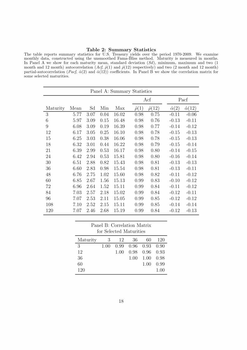
Table 2: Summary StatisticsThe table reports summary statistics for U.S. Treasury yields over the period 1970-2009. We examinemonthly data, constructed using the unsmoothed Fama-Bliss method. Maturity is measured in months.In Panel A we show for each maturity mean, standard deviation (Sd), minimum, maximum and two (1month and 12 month) autocorrelation (Acf, �̂(1) and �̂(12) respectively) and two (2 month and 12 month)partial-autocorrelation (Pacf, �̂(2) and �̂(12)) coefficients. In Panel B we show the correlation matrix forsome selected maturities.

Panel A: Summary Statistics

Acf Pacf

Maturity Mean Sd Min Max �̂(1) �̂(12) �̂(2) �̂(12)3 5.77 3.07 0.04 16.02 0.98 0.75 -0.11 -0.066 5.97 3.09 0.15 16.48 0.98 0.76 -0.13 -0.119 6.08 3.09 0.19 16.39 0.98 0.77 -0.14 -0.1212 6.17 3.05 0.25 16.10 0.98 0.78 -0.15 -0.1315 6.25 3.03 0.38 16.06 0.98 0.78 -0.15 -0.1318 6.32 3.01 0.44 16.22 0.98 0.79 -0.15 -0.1421 6.39 2.99 0.53 16.17 0.98 0.80 -0.14 -0.1524 6.42 2.94 0.53 15.81 0.98 0.80 -0.16 -0.1430 6.51 2.88 0.82 15.43 0.98 0.81 -0.13 -0.1336 6.60 2.83 0.98 15.54 0.98 0.81 -0.13 -0.1148 6.76 2.75 1.02 15.60 0.98 0.82 -0.11 -0.1260 6.85 2.67 1.56 15.13 0.99 0.83 -0.10 -0.1272 6.96 2.64 1.52 15.11 0.99 0.84 -0.11 -0.1284 7.03 2.57 2.18 15.02 0.99 0.84 -0.12 -0.1196 7.07 2.53 2.11 15.05 0.99 0.85 -0.12 -0.12108 7.10 2.52 2.15 15.11 0.99 0.85 -0.14 -0.14120 7.07 2.46 2.68 15.19 0.99 0.84 -0.12 -0.13

Panel B: Correlation Matrixfor Selected Maturities

Maturity 3 12 36 60 1203 1.00 0.99 0.96 0.93 0.9012 1.00 0.98 0.96 0.9336 1.00 1.00 0.9860 1.00 0.99120 1.00

18

DFM and to keep the VAR(k) coefficient matrices unrestricted, we restrict the three rows

corresponding to maturities of 1 (first row), 30 (ninth row) and 120 months (last row) in Λ.

In particular, this set of three rows is set equal to

�1,⋅ = (1, 1, 0), �9,⋅ = (1,1

2, 1), �17,⋅ = (1, 0, 0). (14)

These restrictions facilitate comparison with the factors of the Nelson-Siegel yield curve in

section 3.4 to some extent while the set of restrictions is not singular. We have noticed

that the estimation results are not qualitatively different when we consider another set of

restrictions (for example, the rows of the identity matrix I3) since we can rotate the factors

such that another set of restrictions is implied. The dynamic specification for the three

factors in ft are modelled jointly by a vector autoregressive process of lag order 1 and is

given by

ft+1 = Φft + �t, �t ∼ NID(0, Q), t = 1, . . . , n, (15)

which can be expressed as in (3) with �� = 0, T = Φ, R = I and �t = ft. We denote

this model by VAR(1). In our empirical study, we consider the VAR(1) specification for the

factor process in all model specifications. This choice is the same as in related studies such

as Diebold, Rudebusch, and Aruoba (2006); the exception is Bowsher and Meeks (2008)

where a cointegrated VAR system with multiple lags is considered for the factors.

The maximum likelihood estimates of the factor loadings are presented in the three

columns of Panel A of Table 3. It shows that the loadings associated with the first factor are

very close to unity and therefore we can interpret the first factor as the level. The loading

estimates for the second factor are smoothly descending from one to zero for interest rates

of ascending maturity. This is the typical Nelson and Siegel (1987) shape for their second

factor which they associate with the slope of the yield curve. Their third factor is designed as

the curvature of the yield curve with the associated loading pattern given by an asymmetric,

reverse U-shape. Our loading estimates for the third factor also admit to this pattern and

therefore we can interpret the third factor in ft as the curvature of the yield curve at time t.

How close our estimated loadings are to the Nelson-Siegel loadings is discussed in section 3.4.

In case of the DFM, the loading restrictions in (14) have facilitated the level-slope-curvature

(LSC) interpretation of the three factors. When other loading restrictions were considered,

the estimation results are not different since appropriate factor rotations can be carried out

to obtain the same loadings as presented in Table 3.

19

Table 3: Selection of SDFM SpecificationsThis table shows the factor loading matrix for the DFM and SDFM specifications. We select the knots in the SDFM using both the iterative LRand Wald test procedures. Numbers in italics indicate that no knot is estimated at the location, but the value is interpolated using the splinefor the corresponding column. Asterisks (∗/∗∗) indicate whether the probability of the null (the knot is not necessary) is lower than 5%/1%.

Factor Loading Matrix of DFM and SDFM

Loadings DFM Loadings SDFM, Wald Loadings SDFM, LR

Maturity Factor 1 Factor 2 Factor 3 Factor 1 Factor 2 Factor 3 Factor 1 Factor 2 Factor 3

3 1.000 1.000 0.000 1.000∗∗ 1.000∗∗ 0.000∗∗ 1.000∗∗ 1.000∗∗ 0.000∗∗

6 1.009 0.973 0.253 0.999 0.964 0.241 1.013 0.956 0.2139 1.013 0.917 0.439 0.999 0.917 0.469∗∗ 1.016∗∗ 0.905 0.42312 1.005 0.850 0.645 1.001∗ 0.848∗∗ 0.668 1.007∗∗ 0.841∗∗ 0.628∗∗

15 1.006 0.764 0.829 1.004∗ 0.761∗∗ 0.821∗∗ 1.007 0.763 0.807∗∗

18 1.012 0.700 0.890 1.008 0.700∗∗ 0.913 1.015 0.691∗ 0.88921 1.017 0.645 0.918 1.010 0.647∗∗ 0.960 1.017∗∗ 0.643∗ 0.91224 1.008 0.595 0.946 1.007∗∗ 0.594∗∗ 0.981 1.009 0.592∗∗ 0.942∗∗

30 1.000 0.500 1.000 1.000∗∗ 0.500∗∗ 1.000∗∗ 1.000∗∗ 0.500∗∗ 1.000∗∗

36 1.002 0.424 0.957 0.999∗∗ 0.426∗∗ 1.000∗∗ 1.001∗∗ 0.426∗∗ 0.96548 1.004 0.301 0.852 0.999 0.304∗∗ 0.879∗∗ 1.000 0.304∗∗ 0.85660 0.997 0.212 0.729 1.000 0.211∗∗ 0.741∗∗ 0.997∗∗ 0.215∗∗ 0.742∗∗

72 1.003 0.138 0.636 1.000 0.140∗∗ 0.661∗∗ 0.995 0.146 0.649∗∗

84 0.997 0.091 0.470 1.000 0.088∗∗ 0.473∗∗ 0.995 0.088 0.49096 1.002 0.039 0.316 1.000 0.040∗∗ 0.329∗∗ 0.996 0.045∗∗ 0.335∗∗

108 1.007 0.014 0.192 1.000 0.012 0.213∗∗ 0.998 0.018 0.226∗∗

120 1.000 0.000 0.000 1.000∗∗ 0.000∗∗ 0.000∗∗ 1.000∗∗ 0.000∗∗ 0.000∗∗

20

Table 4: Estimated Transition and Variance MatricesIn these two tables we present the eigenvalues of the estimated transition matrices for the DFM and SDFMmodel, obtained using the iterative LR test procedure. The column with heading ‘real’ contains the real partof the eigenvalues and the column with heading ‘img.’ contains the imaginary parts. Eigenvalues are sortedin ascending order. In Panel A we report results for the DFM model, in Panel B for the SDFM model.

Panel A: Transition and Variance Matrix for DFM

Transition Matrix Eigenvalues Variance Matrix

�1,t−1 �2,t−1 �3,t−1 # real img. �1,t �2,t �3,t

�1,t 0.995 0.018 -0.063 1 0.929 -0.004 0.112 0.018 0.016�2,t -0.009 0.963 0.140 2 0.929 0.000 0.018 0.150 -0.012�3,t 0.009 -0.006 0.891 3 0.991 0.004 0.016 -0.012 0.026

Panel B: Transition and Variance Matrix for SDFM

Transition Matrix Eigenvalues Variance Matrix

�1,t−1 �2,t−1 �3,t−1 # real img. �1,t �2,t �3,t

�1,t 0.995 0.017 -0.063 1 0.929 -0.004 0.112 0.018 0.015�2,t -0.009 0.963 0.141 2 0.929 0.000 0.018 0.154 -0.012�3,t 0.008 -0.006 0.891 3 0.991 0.004 0.015 -0.012 0.026

The autoregressive coefficient matrix Φ and the variance matrix Q in (15) are estimated

jointly with �y, Λ and H in (1) by the method of maximum likelihood. The estimates for

Φ and Q are presented in Panel A of Table 4. The leading diagonal of the estimated Φ

contains values between 0.995 and 0.89 while the off-diagonal elements are all smaller than

0.15 in absolute value. It indicates that the factors are highly persistent over time. To

provide a further insight in the dynamic persistence of the factors, we report the eigenvalues

of the estimated autoregression matrix Φ in Table 4. The two eigenvalues of 0.99 and

0.93 are close to one and have a small imaginary part while one eigenvalue of 0.93 has no

imaginary component. We can therefore view the factors as a weighted sum of one persistent

autoregressive process and two persistent (weakly) cyclical processes.

3.3 Estimation results for smooth loadings

Next we analyze the results that we obtain by applying the method of section 2.4 for finding

a suitable set of smoothness restrictions for the factor loadings of the DFM model. To

ensure that the loadings in the SDFM are identified, we impose the same loading restrictions

21

(14) as for the DFM. Although the estimation results for the DFM are not sensitive to

different restriction choices, once we start to interpolate factor loadings, the positions of

the restrictions can affect the optimal smoothing conditions. We let the restrictions (14)

correspond to the 3, 30, and 120 months of maturities. The interpolating cubic spline

framework requires knot positions at the begin- and end-points (3 and 120 months) while

the knot position of 30 months remains fixed during the selection procedure. However, the

selection procedure can be repeated after moving the knot of 30 months to another time

to maturity. After some experimentation, we have verified that our main results are not

sensitive to moving this knot for 30 months to neighbouring times to maturity.

In the final six columns of Table 3 we present the estimated loadings that are based on

knot positions obtained from the knot selection procedures of sections 2.4, 2.5 and 2.6. At

the start of the procedure, we consider the unrestricted DFM for which 12 out of 42 loading

coefficients (or knots) are significant at the 5% significance level (results omitted for brevity,

but available upon request). This suggests that the number of parameters can be reduced

without affecting the fit significantly. However, the test statistics are strongly correlated and

removing one knot will change the test statistics for the neighbouring knots. We therefore

proceed by sequentially removing the knot with the lowest Wald-statistic and re-estimating

the model after each step, see section 2.4. This “general to specific” procedure is terminated

when all test statistics for the remaining knots are significant at the 5% significance level. The

middle three columns show the smooth dynamic factor model obtained from this procedure.

In addition, we consider a specific to general selection procedure that is based on a hybrid

approach of merging the Lagrange multiplier procedure of section 2.5 and likelihood ratio

statistic procedure of section 2.6 which starts with the most parsimonious model based on

knot values implied by the loading restrictions (14). By subsequently adding a knot at

positions where the restriction is rejected most strongly, we obtain the hybrid “specific to

general” procedure as also described in section 2.7. We refer to this approach as the LR test

procedure.

To let a cubic spline fit a certain shape, the distribution of the knots is generally more

important than the exact location of the knots. First, we look at the knot selection procedure

based on the Wald statistics. We find that the selection procedure is successful in fitting the

first column of factor loadings, as the fourth column of Table 3 is close to the first column

from the DFM. The original set of 14 unrestricted loading parameters is reduced to four

remaining knot parameters. Given that all original estimates are close to unity, this result

may not be surprising. Overall, we reduced the number of parameters in the loading matrix

Λ by 18, a reduction of 43 percent. The resulting values for the loadings are close to those

of the DFM in Panel A. The results for our second LR selection procedure are presented in

22

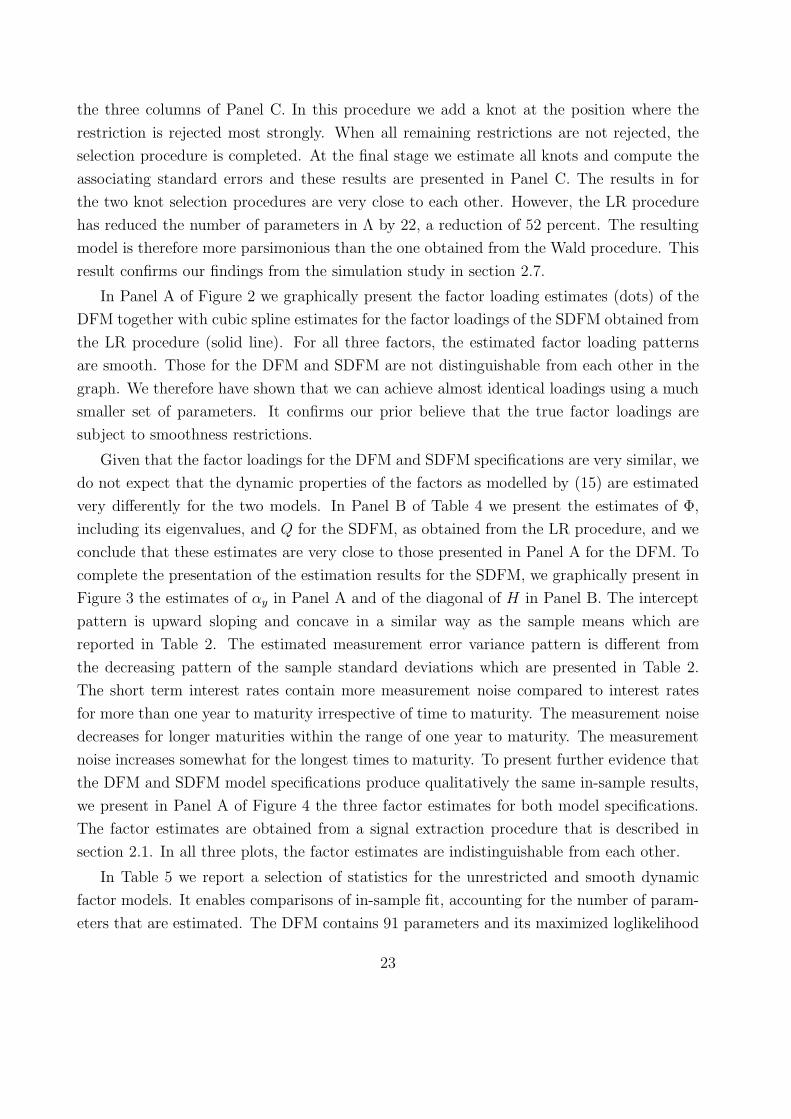
the three columns of Panel C. In this procedure we add a knot at the position where the

restriction is rejected most strongly. When all remaining restrictions are not rejected, the

selection procedure is completed. At the final stage we estimate all knots and compute the

associating standard errors and these results are presented in Panel C. The results in for

the two knot selection procedures are very close to each other. However, the LR procedure

has reduced the number of parameters in Λ by 22, a reduction of 52 percent. The resulting

model is therefore more parsimonious than the one obtained from the Wald procedure. This

result confirms our findings from the simulation study in section 2.7.

In Panel A of Figure 2 we graphically present the factor loading estimates (dots) of the

DFM together with cubic spline estimates for the factor loadings of the SDFM obtained from

the LR procedure (solid line). For all three factors, the estimated factor loading patterns

are smooth. Those for the DFM and SDFM are not distinguishable from each other in the

graph. We therefore have shown that we can achieve almost identical loadings using a much

smaller set of parameters. It confirms our prior believe that the true factor loadings are

subject to smoothness restrictions.

Given that the factor loadings for the DFM and SDFM specifications are very similar, we

do not expect that the dynamic properties of the factors as modelled by (15) are estimated

very differently for the two models. In Panel B of Table 4 we present the estimates of Φ,

including its eigenvalues, and Q for the SDFM, as obtained from the LR procedure, and we

conclude that these estimates are very close to those presented in Panel A for the DFM. To

complete the presentation of the estimation results for the SDFM, we graphically present in

Figure 3 the estimates of �y in Panel A and of the diagonal of H in Panel B. The intercept

pattern is upward sloping and concave in a similar way as the sample means which are

reported in Table 2. The estimated measurement error variance pattern is different from

the decreasing pattern of the sample standard deviations which are presented in Table 2.

The short term interest rates contain more measurement noise compared to interest rates

for more than one year to maturity irrespective of time to maturity. The measurement noise

decreases for longer maturities within the range of one year to maturity. The measurement

noise increases somewhat for the longest times to maturity. To present further evidence that

the DFM and SDFM model specifications produce qualitatively the same in-sample results,

we present in Panel A of Figure 4 the three factor estimates for both model specifications.

The factor estimates are obtained from a signal extraction procedure that is described in

section 2.1. In all three plots, the factor estimates are indistinguishable from each other.

In Table 5 we report a selection of statistics for the unrestricted and smooth dynamic

factor models. It enables comparisons of in-sample fit, accounting for the number of param-

eters that are estimated. The DFM contains 91 parameters and its maximized loglikelihood

23

Figure 2: Estimated Factor Loadings for DFM and SDFM ModelThis figure shows the estimated factor loadings as functions of time to maturity for the optimal SDFMmodel, obtained using the iterative LR test procedure. For ease of comparison we also show the maximumlikelihood estimates of the loadings in the DFM model. The loadings are restricted with the rows of theidentity matrix at the 3 months, 30 months and 120 months maturities. Panel (A) plots the factor loadingsas estimated for the DFM and SDFM, together with those of the Nelson-Siegel model for reference. Panel(B) shows the factor loadings from Panel (A) rotated towards the factor loadings of the Nelson-Siegel model.

(A) Factor Loadings of DFM, SDFM and NS

DFM SDFM NS(0.0609)

10 20 30 40 50 60 70 80 90 100 110 120

1.0

1.1 Loading of Factor 1DFM SDFM NS(0.0609)

DFM SDFM NS(0.0609)

10 20 30 40 50 60 70 80 90 100 110 120

0.5

1.0 Loading of Factor 2DFM SDFM NS(0.0609)

DFM SDFM NS(0.0609)

10 20 30 40 50 60 70 80 90 100 110 120

0.5

1.0 Loading of Factor 3DFM SDFM NS(0.0609)

(B) DFM and SDFM Loadings rotated to NS

DFM Rotated SDFM Rotated NS(0.0609)

10 20 30 40 50 60 70 80 90 100 110 120

1.0

1.1 Loading of Factor 1DFM Rotated SDFM Rotated NS(0.0609)

DFM Rotated SDFM Rotated NS(0.0609)

10 20 30 40 50 60 70 80 90 100 110 120

0.25

0.50

0.75

1.00 Loading of Factor 2

DFM Rotated SDFM Rotated NS(0.0609)

DFM Rotated SDFM Rotated NS(0.0609)

10 20 30 40 50 60 70 80 90 100 110 120

0.1

0.2

0.3 Loading of Factor 3DFM Rotated SDFM Rotated NS(0.0609)

24

Figure 3: Intercept and Measurement Error VarianceIn this figure we show the intercept and measurement error variance as functions of time to maturity fromthe SDFM model, obtained using the iterative LR test procedure. For ease of comparison we also show thesefor the DFM model.

(A) Intercepts

DFM × Maturities SDFM × Maturities

10 20 30 40 50 60 70 80 90 100 110 120

6.2

6.4

6.6

6.8

7.0

7.2

7.4 Intercepts

DFM × Maturities SDFM × Maturities

(B) Measurement Error Variance

DFM × Maturities SDFM × Maturities

10 20 30 40 50 60 70 80 90 100 110 120

0.01

0.02

0.03

0.04

0.05

0.06

0.07

Measurement Error Variance

DFM × Maturities SDFM × Maturities

Figure 4: Smoothed Factors for DFM and SDFM ModelIn this figure we show the smoothed time series of the latent factors for the SDFM model, obtained usingthe iterative LR test procedure. For ease of comparison we also show these for the DFM model in the samefigures, and of the Nelson-Siegel model in the right figures.

SDFM DFM

1970 1980 1990 2000 2010

0

5

Factor 1SDFM DFM

NS

1970 1980 1990 2000 2010

5

10

15NS

SDFM DFM

1970 1980 1990 2000 2010

−2.5

0.0

2.5

5.0 Factor 2SDFM DFM

NS

1970 1980 1990 2000 2010−5

0

5 NS

SDFM DFM

1970 1980 1990 2000 2010−1

0

1Factor 3

SDFM DFM

NS

1970 1980 1990 2000 2010

−5

0

5 NS

25

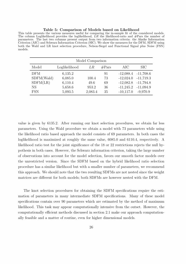
Table 5: Comparison of Models based on LikelihoodThis table presents the various measures useful for comparing the in-sample fit of the considered models.The column Loglikelihood provides the loglikelihood, LR the likelihood-ratio and #Pars the number ofparameters. The last two columns present output from two information criteria: the Akaike InformationCriterion (AIC) and Schwarz Information Criterion (SIC). We show the measures for the DFM, SDFM usingboth the Wald and LR knot selection procedure, Nelson-Siegel and Functional Signal plus Noise (FSN)models.

Model Comparison

Model Loglikelihood LR #Pars AIC SIC

DFM 6,135.2 91 -12,088.4 -11,708.6SDFM(Wald) 6,085.0 100.4 73 -12,024.0 -11,719.3SDFM(LR) 6,110.4 49.6 69 -12,082.8 -11,794.8NS 5,658.6 953.2 36 -11,245.2 -11,094.9FSN 5,093.5 2,083.4 35 -10,117.0 -9,970.9

value is given by 6135.2. After running our knot selection procedures, we obtain far less

parameters. Using the Wald procedure we obtain a model with 73 parameters while using

the likelihood ratio based approach the model consists of 69 parameters. In both cases the

loglikelihood is maximized at roughly the same value, 6085.0 and 6110.4, respectively. A

likelihood ratio test for the joint significance of the 18 or 22 restrictions rejects the null hy-

pothesis in both cases. However, the Schwarz information criterion, taking the large number

of observations into account for the model selection, favors our smooth factor models over

the unrestricted version. Since the SDFM based on the hybrid likelihood ratio selection

procedure has a similar likelihood but with a smaller number of parameters, we recommend

this approach. We should note that the two resulting SDFMs are not nested since the weight

matrices are different for both models; both SDFMs are however nested with the DFM.

The knot selection procedures for obtaining the SDFM specifications require the esti-

mation of parameters in many intermediate SDFM specifications. Many of these model

specifications contain over 90 parameters which are estimated by the method of maximum

likelihood. This task may appear computationally intensive from the outset. However, the

computationally efficient methods discussed in section 2.1 make our approach computation-

ally feasible and a matter of routine, even for higher dimensional models.

26

3.4 Comparisons with the Nelson-Siegel yield curve

In an important contribution Nelson and Siegel (1987) have shown that the term structure

can surprisingly well be fitted by a linear combination of three smooth functions. The

Nelson-Siegel yield curve is then given by

fL + �S(�) ⋅ fS + �C(�) ⋅ fC , (16)

where fL, fS and fC are treated as the level, slope and curvature (LSC) factors, respectively,

and the corresponding factor weights for slope and curvature are functions of time to maturity

� , that is

�S(�) =1− e−��

��, �C(�) =

1− e−��

��− e−�� , (17)

with unknown coefficient � > 0. The interpretation of the LSC factors is obtained as

follows. The factor fL is by construction the overall level of the yield curve. The factor fS is

associated with the slope of the yield curve since its loading �S(�) is high for a short maturity

� and low for a long maturity. The loadings �C(�) is an inverted U-shaped function of �

and therefore fC can be interpreted as the curvature of the yield. The decomposition of the

yield curve into these LSC factors has also been highlighted by Litterman and Scheinkman

(1991).

The LSC factors fL, fS, fC and the coefficient �, are treated as parameters which can be

estimated at each time t by a least squares method based on the nonlinear regression model

yit = fL + �S(�i) ⋅ fS + �C(�i) ⋅ fC + uit, i = 1, . . . , N,

where yit is the interest rate at time t for time to maturity �i and where uit is a noise

term with zero mean and possibly different variances for different times to maturity �i, for

i = 1, . . . , N .

The Nelson-Siegel yield curve can also be incorporated in a dynamic factor model by

placing the LSC factors into the vector f̃t and to let them evolve as a time-varying process.

We obtain

yt = �y + Λnsf̃t + "t, "t ∼ NID(0, H), (18)

where the 3 × 1 vector f̃t represents the LSC factors and is modelled as a VAR(1) process

as in (15) while H is a diagonal variance matrix. The ith row of the loading matrix Λns is

given by [1 , �S(�i) , �C(�i)]. The resulting dynamic Nelson-Siegel (DNS) model can also be

regarded as a smooth dynamic factor model in which the smoothness in the loading matrix

is determined by the functional form (17) and parameter �. The loading matrix Λns depends

27

on a single parameter � and is therefore more restrictive than the SDFM. The DNS model is

proposed by Diebold, Rudebusch, and Aruoba (2006). Their specification is slightly different

as they set �y in (18) to zero and include an intercept in the specification (15) for f̃t.

The DNS model can clearly also be represented in the state space form (1)–(3) and we

can estimate the parameters of the model as described in section 2.1. We follow the practice

of Diebold, Rudebusch, and Aruoba (2006) by setting � fixed at 0.0609. The remaining

parameters in the DNS are estimated for the data set of section 3.1. In Panel A of Figure

2 the DNS loadings are presented as a dotted line and can be compared with those for the

DFM and SDFM. Although the shapes of the loading patterns are similar, the loading values

from the DNS model are clearly different. However, we can rotate the factors in the DFM

and SDFM in such a way that the loadings become very close to those of the Nelson-Siegel

loadings. The result of the DFM and SDFM loading rotations are presented in Panel B and

we can conclude that the DFM and SDFM can approximate the LSC factors from the DNS

model with a high degree of precision. Whether the results for in-sample and out-of-sample

fit are different for the different models will be discussed next.

The differences between the extracted factors from the SDFM (not rotated to DNS) and

from the DNS model can be detected when comparing the plots in on the left to those on

the right of Figure 4. The level and scale of the SDFM and DNS factors are different which

is due to the different estimates of �y and factor loadings themselves. However, the paths of

the factors through time for the two different models are very similar. Finally, Table 5 also

reports the optimized likelihood and information criteria for the Nelson-Siegel model. The

model produces a far lower loglikelihood value such that it has a far higher LR compared to

the smooth factor models. The information criteria take the far lower number of parameters

into account (36 in the Nelson-Siegel model compared to 91 in the DFM), but still favor

the dynamic factor models over the Nelson-Siegel model. A possible explanation for why

the factors and loadings appear similar in the models but result in very different likelihood

values, is the high precision with which the model is estimated. In additional results, we

show that the confidence intervals around the estimated loadings are very narrow. It implies

that small perturbations in the maximum likelihood estimates will cause large changes in

the loglikelihood value.

3.5 Comparisons with the spline yield curve

A recent alternative for the Nelson-Siegel yield curve is proposed by Bowsher and Meeks

(2008) who adopt the cubic spline function for describing the smooth term structure of

interest rates. They have labelled their approach as the functional signal plus noise (FSN)

28

model. The modelling of the smooth signal vector Λft directly in terms of a cubic spline

function is discussed in section 2.3. The spline yield curve is based on the observation

equation given by

yt = W ′f̄t + "t, f̄t = Z�t, (19)

where the spline weight matrix W and the coefficient vector f̄t are defined in section 2.3, the

time-varying specification f̄t = Z�t replaces (2) and the dynamic specification for �t is given

by (3). To facilitate comparisons with DFM, SDFM and DNS in the context of interest rate

series for different times to maturity, we consider three factors in f̄t. For the construction of

the spline through times of maturity and the corresponding spline weights in W , we place

knots at the positions 3, 30 and 120 months to maturity. Hence we can interpret the three

factors in f̄t as factors representing interest rates associated with the short, medium and

long times to maturity. This interpretation of f̄t deviates from the LSC interpretation of

the Nelson-Siegel factors. Given the construction of the cubic spline weights in which the

columns ofW at the knot positions equal the identity matrix, we can provide the three factors

of the FSN spline yield coefficients in f̄t with a LSC interpretation. By pre-multiplying W

with the matrix B = [�′1,⋅, �

′9,⋅, �

′17,⋅] where �j,⋅ is defined in (14) for j = 1, 9, 17, we obtain

the loading matrix Wlsc = BW which leads to the LSC interpretation of the factors in f̄t

that determine the spline yield curve W ′lscf̄t. The interpretation follows immediately since

the jth column of W equals �j,⋅ for j = 1, 9, 17.

Table 5 also reports the optimized likelihood and information criteria for the FSN model.

The number of parameters is further reduced to 35, asW contains no parameters but is solely

determined by the positions of the knots. Similar to the Nelson-Siegel model, the FSN model

produces a loglikelihood that is far lower than the smooth factor models. The information

criteria also do not favor this model. When compared to the Nelson-Siegel model, the FSN

likelihood is also lower.

3.6 Forecasting results

To investigate the out-of-sample fit for the DFM, SDFM, DNS and FSN specifications for

our panel time series of U.S. interest rates, we carry out a forecasting exercise. We forecast

the full yield curve (the interest rates for 17 times to maturity) up to 24 months ahead.

We forecast the yield curve for the months from January 1994 up to December 2009. To

obtain the 24 month ahead forecast of the yield curve for January 1994, we estimate the

parameters in the four different models using the observations of the time series panel from

January 1970 up to January 1992. The 23 month ahead forecast for January 1994 and the

24 month ahead forecast for February 1994 are obtained by estimating the parameters in

29

the four different models based on the data from January 1970 up to February 1992. In this

way we compute the forecasts, and the corresponding forecast errors, for ℎ = 1, 6, 12, 18, 24

months ahead. We record the forecast errors for each forecast horizon, for each maturity

and for each model. Then we compute the root mean square forecast error (RMSFE) for all

these cases. The results of this extensive forecasting study are partially reported in Table 6.

The re-estimation of the parameters in the different models is an extensive numerical task

but it remains feasible when using the methods discussed in section 2.1. For simplicity, we

fix the number of knots for different sample periods and we also keep the knot positions as

obtained from the knot selection procedure based on the LR test. The selection is based

on the full sample. Alternative strategies where we, for example, yearly repeat the knot

selection procedure have yielded similar forecasting results.

In Panel A of Table 6 we report the forecasting results for the expanding window by

means of the RMSFEs for the times to maturity 3, 12, 36, 60, 120 months. The one-month

ahead forecasts for the 3-month interest rate is clearly the lowest for the forecasts produced

by the SDFM while for the other times to maturity the RMSFE are more or less equal for

all models. The multiple-months ahead forecasts produced by the SDFM have RMSFEs

that are comparable to those from the DFM. The smoothing restrictions imposed by the

DNS appear to lead to somewhat higher RMSFEs throughout except for one-year interest

rates although in this case the differences are small. The FSN model provides RMSFEs

that are particularly favorably in intermediate maturities at the short horizon. In Panel

B we examine the robustness of the forecasting improvement. We show the RMSFEs for

the periods 1994-1998, 1999-2003 and 2004-2009. We can observe some variation over these

periods, the SDFM forecast precision are comparable to, or even better than, those of the

Nelson-Siegel model. In the first two subsamples the SDFM produces the lowest RMSFEs,

while in the last subsample the FSN model performs remarkably well but the differences

are small in all subsamples. We can conclude that the smoothing restrictions imposed on

the DFM do not affect the precision of the forecasts and often achieve the highest precision.

These results are of course relative to our newly constructed data set of U.S. interest rates.

30

Table 6: Forecasting Performance of Factor ModelsIn these tables we present the forecasting performance of the various models. We show the root mean squareforecast error (RMSFE) for the SDFM with knots from the LR procedure, the general DFM, Nelson-Siegelin SSF (NS-SSF) and and Functional Signal plus Noise (FSN) models. In Panel A we show results for the1994-2009 sample, in Panel B for three different subperiods (1994-1998, 1999-2003 and 2004-2009). For eachmodel the RMSFE is reported for 3 month, 1, 3, 5 and 10 year maturities, and ℎ=1, 6, 12, 18 and 24-monthahead forecasts.

Panel A: Forecasting Performance 1994-20093 month 1 year 3 year 5 year 10 year

SDFMℎ=1 0.314 0.274 0.321 0.314 0.304ℎ=6 0.956 1.009 0.959 0.869 0.678

ℎ=12 1.615 1.628 1.426 1.243 0.939

ℎ=18 2.096 2.068 1.758 1.507 1.101

ℎ=24 2.438 2.396 2.026 1.734 1.275

DFMℎ=1 0.328 0.273 0.320 0.315 0.300ℎ=6 0.959 1.008 0.958 0.871 0.679ℎ=12 1.614 1.626 1.426 1.246 0.943ℎ=18 2.094 2.067 1.759 1.512 1.110ℎ=24 2.435 2.397 2.028 1.741 1.288

NS-SSFℎ=1 0.347 0.271 0.321 0.319 0.293

ℎ=6 0.998 1.004 0.965 0.878 0.696ℎ=12 1.671 1.622 1.440 1.259 0.981ℎ=18 2.166 2.064 1.781 1.532 1.169ℎ=24 2.526 2.400 2.061 1.772 1.367

FSNℎ=1 0.379 0.265 0.316 0.310 0.295ℎ=6 0.969 0.989 0.953 0.886 0.721ℎ=12 1.665 1.614 1.437 1.281 1.010ℎ=18 2.183 2.073 1.803 1.581 1.205ℎ=24 2.553 2.414 2.091 1.827 1.393

31

Panel B: Forecasting Performance for SubperiodsForecasting Performance 1994-1998 Forecasting Performance 1999-2003 Forecasting Performance 2004-2009

3 month 1 year 3 year 5 year 10 year 3 month 1 year 3 year 5 year 10 year 3 month 1 year 3 year 5 year 10 yearSDFMℎ=1 0.153 0.252 0.279 0.290 0.311 0.280 0.300 0.352 0.343 0.298 0.422 0.268 0.326 0.307 0.303ℎ=6 0.483 0.715 0.783 0.798 0.771 1.112 1.216 1.084 0.949 0.673 1.101 1.028 0.979 0.855 0.595

ℎ=12 0.758 0.940 1.013 1.035 1.005 1.932 2.020 1.666 1.399 0.974 1.836 1.711 1.502 1.262 0.848

ℎ=18 0.850 0.949 0.999 1.032 0.999 2.493 2.548 2.056 1.703 1.186 2.437 2.289 1.972 1.658 1.108

ℎ=24 0.938 0.968 0.961 0.992 0.937 2.877 2.931 2.397 2.010 1.469 2.866 2.714 2.321 1.957 1.345

DFMℎ=1 0.154 0.252 0.279 0.294 0.303 0.305 0.299 0.350 0.343 0.297 0.435 0.267 0.326 0.309 0.300ℎ=6 0.477 0.715 0.784 0.801 0.770 1.118 1.214 1.083 0.950 0.674 1.105 1.027 0.978 0.858 0.596ℎ=12 0.755 0.941 1.015 1.039 1.007 1.931 2.019 1.666 1.403 0.980 1.834 1.708 1.499 1.264 0.852ℎ=18 0.850 0.951 1.003 1.039 1.007 2.493 2.550 2.060 1.711 1.200 2.431 2.286 1.969 1.660 1.114ℎ=24 0.942 0.975 0.968 1.004 0.952 2.877 2.935 2.402 2.021 1.486 2.860 2.712 2.320 1.960 1.352

NS-SSFℎ=1 0.185 0.244 0.279 0.289 0.275 0.289 0.301 0.354 0.353 0.309 0.472 0.266 0.325 0.313 0.293

ℎ=6 0.559 0.710 0.787 0.799 0.767 1.150 1.217 1.098 0.964 0.717 1.138 1.017 0.980 0.866 0.610ℎ=12 0.843 0.940 1.021 1.042 1.018 2.004 2.027 1.697 1.428 1.054 1.872 1.689 1.503 1.274 0.882ℎ=18 0.966 0.968 1.028 1.059 1.049 2.595 2.565 2.105 1.749 1.299 2.474 2.259 1.971 1.665 1.149ℎ=24 1.127 1.042 1.046 1.069 1.055 3.004 2.958 2.461 2.071 1.600 2.905 2.676 2.317 1.960 1.387

FSNℎ=1 0.467 0.266 0.289 0.305 0.284 0.319 0.287 0.334 0.334 0.299 0.341 0.245 0.323 0.294 0.300ℎ=6 0.730 0.782 0.867 0.903 0.844 1.094 1.169 1.034 0.932 0.688 1.031 0.978 0.952 0.830 0.632ℎ=12 1.004 1.031 1.133 1.189 1.123 2.026 2.017 1.670 1.432 1.031 1.769 1.633 1.454 1.219 0.886ℎ=18 1.157 1.083 1.159 1.232 1.168 2.655 2.593 2.134 1.809 1.310 2.393 2.209 1.937 1.636 1.143ℎ=24 1.325 1.173 1.195 1.256 1.172 3.058 2.980 2.490 2.128 1.610 2.852 2.644 2.302 1.953 1.368

32

4 Conclusion

In this paper we have developed a maximum likelihood procedure for imposing smoothing

restrictions on the loading matrix of a dynamic factor model. We have used cubic spline

functions to introduce smoothness in factor loadings. For a newly updated time series panel

of unsmoothed Fama-Bliss zero yields for U.S. treasuries, we show that it is possible to

construct a parsimonious dynamic factor model with smooth factor loadings. The number

of parameters in the loading matrix of the dynamic factor model is more or less halved.

Despite of this reduction in the number of parameters we find that the in-sample fit of our

model is qualitatively the same as for the most general dynamic factor model. We can rotate

the factor loadings in such a way that the factors are given the level, slope and curvature

interpretation of the Nelson-Siegel yield curve. Our forecasting study has shown that smooth

dynamic factor models are highly competitive in producing precise forecasts of the yield curve

for a range of forecast horizons, from 1 month to 24 months.

Although the analysis of the U.S. term structure of interest rates is highly relevant

in finance and economics, we emphasize that dynamic factor models with smooth factor

loadings can be used in different settings. In many applications of the dynamic factor model

it is possible to identify variables of which the factor loadings can reasonably be assumed

to behave as smooth functions. An example is the modelling and forecasting of intra-daily

electricity load consumption curves. Our methodology provides means to build parsimonious

dynamic factor models for even high dimensional time series panels and with factors that

can be given a clear interpretation. We will explore this methodology further in future work.

Appendix

The dynamic factor model is given by equations (1), (2) and (3) for a panel of N time series

and r factors. When we introduce lagged factors in the observation equation (1), the model

becomes

yt = �y + Λ0ft + Λ1ft−1 + . . .+ Λsft−s + "t,

where Λm is an N × r loading matrix for m = 0, 1, . . . , s and where ft = Z�t and �t remain

specified as (2) and (3), respectively, for some pre-fixed integer s > 0. This model can still

be written in state space after some modifications. We do not want to increase the state

vector unnecessarily and therefore we propose the following formulation. An efficient state

space representation for the model with lagged factors can be based on the state vector as

33

defined by

�∗t =

(�′t , f

′t−1 , . . . , f

′t−s+1 , f

′t−s

)′,

where �t remains as in (3). For the state vector �∗t , the observation equation becomes

yt = �y + (Λ0Z , Λ1 , . . . , Λs−1 , Λs )�∗t + "t,

and the state updating equation for �∗t becomes

�∗t+1 =

⎛⎜⎜⎜⎜⎜⎜⎝

�y

0

0...

0

⎞⎟⎟⎟⎟⎟⎟⎠

+

⎡⎢⎢⎢⎢⎢⎢⎣

T 0 0 ⋅ ⋅ ⋅ 0 0

Z 0 0 ⋅ ⋅ ⋅ 0 0

0 I 0 ⋅ ⋅ ⋅ 0 0...

. . ....

0 0 0 I 0

⎤⎥⎥⎥⎥⎥⎥⎦�∗t +

⎡⎢⎢⎢⎢⎢⎢⎣

R

0

0...

0

⎤⎥⎥⎥⎥⎥⎥⎦�t,

for t = 1, . . . , n. This representation illustrates the generality of the state space form for

dynamic factor models. The dimension of the state vector �∗t remains relatively small since

we augment �∗t by lagged ft’s rather than lagged �t’s.

References

Bai, J. (2003). Inferential theory for factor models of large dimensions. Econometrica 71,

135–72.

Bliss, R. (1997). Movements in the term structure of interest rates. Federal Reserve Bank

of Atlanta Economic Review 82, 16–33.

Bowsher, C. and R. Meeks (2008). The dynamics of economic functions: modeling and

forecasting the yield curve. J. American Statistical Association 103, 1419–37.

Box, G. E. P., G. M. Jenkins, and G. C. Reinsel (1994). Time Series Analysis, Forecasting

and Control (3rd ed.). San Francisco: Holden-Day.

Christensen, J., F. Diebold, and S. Rudebusch (2010). The affine arbitrage-free class of

Nelson-Siegel term structure models. J. Econometrics (forthcoming).

Clements, M. P. and D. Hendry (1998). Forecasting Economic Time Series. Cambridge:

Cambridge University Press.

Connor, G. and R. A. Korajczyk (1993). A test for the number of factors in an approximate

factor model. Journal of Finance 48 (4), 1263–91.

34

De Pooter, M. (2007). Examining the Nelson-Siegel class of term structure models. Tin-

bergen Institute Discussion Paper.

Diebold, F. and C. Li (2006). Forecasting the term structure of government bond yields.

J. Econometrics 130, 337–64.

Diebold, F., S. Rudebusch, and S. Aruoba (2006). The macroeconomy and the yield curve.

J. Econometrics 131, 309–38.

Doz, C., D. Giannone, and L. Reichlin (2006). A quasi maximum likelihood approach for

large approximate dynamic factor models. Discussion paper, CEPR.

Duffee, G. (2009). Forecasting with the term structure: The role of no-arbitrage restric-

tions. Working paper.

Durbin, J. and S. J. Koopman (2001). Time Series Analysis by State Space Methods.

Oxford: Oxford University Press.

Engle, R. F. (1984, July). Wald, likelihood ratio, and lagrange multiplier tests in economet-

rics. In Handbook of Econometrics, Volume 2 of Handbook of Econometrics, Chapter 13,

pp. 775–826. Elsevier.

Engle, R. F. and M. W. Watson (1981). A one-factor multivariate time series model of

metropolitan wage rates. J. American Statistical Association 76, 774–81.

Fama, E. F. and R. R. Bliss (1987). The information in long-maturity forward rates.

American Economic Review 77, 680–92.

Fengler, M., W. Haerdle, and P. Schmidt (2002). The analysis of implied volatilities. In

W. Haerdle, T. Kleinow, and G. Stahl (Eds.), Applied Quantitative Finance: Theory

and Computational Tools, Chapter 6, pp. 127–37. Berlin: Springer.

Forni, M., M. Hallin, M. Lippi, and L. Reichlin (2000). The generalized dynamic factor

model: Identification and estimation. Rev. Economics and Statistics 82, 540–54.

Geweke, J. (1977). The dynamic factor analysis of economic time series. In D. J. Aigner

and A. S. Goldberger (Eds.), Latent variables in socio-economic models. Amsterdam:

North-Holland.

Gregory, A., A. Head, and J. Raynauld (1997). Measuring world business cycles. Interna-

tional Economic Review 38, 677–701.

Harvey, A. C. and S. J. Koopman (1993). Forecasting hourly electricity demand using

time-varying splines. J. American Statistical Association 88, 1228–36.

35

Jungbacker, B. and S. J. Koopman (2008). Likelihood-based analysis for dynamic factor

models. Tinbergen Institute Discussion Paper.

Koopman, S. J. and J. Durbin (2000). Fast filtering and smoothing for multivariate state

space models. J. Time Series Analysis 21, 281–96.

Koopman, S. J., M. Mallee, and M. Van der Wel (2010). Analyzing the term structure of

interest rates using the dynamic Nelson-Siegel model with time-varying parameters. J.

Business and Economic Statist. 28, 329–343.

Koopman, S. J. and N. Shephard (1992). Exact score for time series models in state space

form. Biometrika 79, 823–6.

Lengwiler, Y. and C. Lenz (2010). Intelligible factors for the yield curve. J. Econometrics

(forthcoming).

Litterman, R. and J. Scheinkman (1991). Common factors affecting bond returns. Journal

of Fixed Income 1 (1), 54–61.

Monahan, J. F. (2001). Numerical methods of statistics. Cambridge: Cambridge University

Press.

Nelson, C. and A. Siegel (1987). Parsimonious modelling of yield curves. Journal of Busi-

ness 60-4, 473–89.

Nocedal, J. and S. J. Wright (1999). Numerical Optimization. New York: Springer Verlag.

Park, B., E. Mammen, W. Haerdle, and S. Borak (2009). Time Series Modelling with

Semiparametric Factor Dynamics. J. American Statistical Association 104, 284–98.

Poirier, D. J. (1976). The Econometrics of Structural Change: with Special Emphasis on

Spline Functions. Amsterdam: North-Holland.

Quah, D. and T. J. Sargent (1993). A dynamic index model for large cross sections. In

J. H. Stock and M. Watson (Eds.), Business cycles, indicators and forecasting, pp.

285–306. Chicago: University of Chicago Press.

Reis, R. and M. W. Watson (2010). Relative goods’ prices, pure inflation, and the phillips

correlation. American Economic Journal: Macroeconomics 2, 128–57.

Sargent, T. J. and C. A. Sims (1977). Business cycle modeling without pretending to have

too much a priori economic theory. In C. A. S. et al. (Ed.), New methods in business

cycle research. Minneapolis: Federal Reserve Bank of Minneapolis.

Stock, J. H. and M. Watson (2002). Macroeconomic forecasting using diffusion indexes.

J. Business and Economic Statist. 20, 147–62.

36

Watson, M. W. and R. F. Engle (1983). Alternative algorithms for the estimation of

dynamic factor, MIMIC and varying coefficient regression. J. Econometrics 23, 385–

400.

37