Dynamic Estimation of Volatility Risk Premia and Investor Risk ...

Finance and Economics Discussion Series Divisions of Research & Statistics and Monetary Affairs

Federal Reserve Board, Washington, D.C.

Dynamic Estimation of Volatility Risk Premia and Investor Risk Aversion from Option-Implied and Realized Volatilities

Tim Bollerslev, Michael Gibson, and Hao Zhou 2004-56

NOTE: Staff working papers in the Finance and Economics Discussion Series (FEDS) are preliminary materials circulated to stimulate discussion and critical comment. The analysis and conclusions set forth are those of the authors and do not indicate concurrence by other members of the research staff or the Board of Governors. References in publications to the Finance and Economics Discussion Series (other than acknowledgement) should be cleared with the author(s) to protect the tentative character of these papers.

Dynamic Estimation of Volatility RiskPremia and Investor Risk Aversion fromOption-Implied and Realized Volatilities∗

Tim Bollerslev†

Michael Gibson‡

Hao Zhou§

First Draft: September 2004

∗The work of Bollerslev was supported by a grant from the National Science Foundation to theNBER. We would like to thank Nellie Liang for useful discussions during this project. The viewspresented here are solely those of the authors and do not necessarily represent those of the FederalReserve Board or its staff. Matthew Chesnes provided excellent research assistance.

†Department of Economics, Duke University, Post Office Box 90097, Durham NC 27708, andNBER, USA, Email [email protected], Phone 919-660-1846, Fax 919-684-8974.

‡Division of Research and Statistics, Federal Reserve Board, Mail Stop 91, Washington DC20551 USA, E-mail [email protected], Phone 202-452-2495, Fax 202-728-5887.

§Division of Research and Statistics, Federal Reserve Board, Mail Stop 91, Washington DC20551 USA, E-mail [email protected], Phone 202-452-3360, Fax 202-728-5887.

Abstract

This paper proposes a method for constructing a volatility risk premium, or investor

risk aversion, index. The method is intuitive and simple to implement, relying on the sam-

ple moments of the recently popularized model-free realized and option-implied volatility

measures. A small-scale Monte Carlo experiment suggests that the procedure works well in

practice. Implementing the procedure with actual S&P500 option-implied volatilities and

high-frequency five-minute-based realized volatilities results in significant temporal depen-

dencies in the estimated stochastic volatility risk premium, which we in turn relate to a set

of underlying macro-finance state variables. We also find that the extracted volatility risk

premium helps predict future stock market returns.

JEL Classification: G12, G13, C51, C52.

Keywords: Stochastic Volatility Risk Premium, Model-Free Implied Volatility, Model-Free

Realized Volatility, Black-Scholes, GMM Estimation, Monte Carlo, Return Predictability.

1 Introduction

Model-free volatility measures have figured prominently in the recent academic and financial

market practitioner literatures. More specifically, several studies have argued for the use

of so-called “model-free realized volatilities” computed by summing squared returns from

high-frequency data over short time intervals during the trading day. As demonstrated in

the literature, these types of measures afford much more accurate ex-post observations of

the actual volatility than the more traditional sample variances based on daily or coarser

frequency data (Andersen et al., 2001; Barndorff-Nielsen and Shephard, 2002; Meddahi, 2002;

Andersen et al., 2003a,b; Barndorff-Nielsen and Shephard, 2004a; Andersen et al., 2004). In

parallel to these results, the recently developed so-called “model-free implied volatilities”

provide ex-ante (risk-neutral) expectations of the future volatilities. Importantly, and in

contrast to more traditional option-implied volatilities which are based on the Black-Scholes

pricing formula or some variant thereof, the model-free implied volatilities are computed

from option prices without the use of any particular option-pricing model (Britten-Jones

and Neuberger, 2000; Jiang and Tian, 2004; Lynch and Panigirtzoglou, 2003).1 In this

paper, we combine these two new volatility measures to improve on existing estimates of the

risk premium associated with stochastic volatility risk and investor risk aversion.

Because the method we present here directly uses the model-free realized and implied

volatilities to extract the stochastic volatility risk premium, it is much easier to implement

than other methods in the literature, which typically rely on the joint estimation of both the

underlying asset return and the price(s) of one or more of its derivatives, leading to quite

complicated modeling and estimation (see, e.g., Bates, 1996; Chernov and Ghysels, 2000;

Benzoni, 2001; Pan, 2002; Eraker, 2004, among many others). In contrast, the method of

this paper relies on GMM estimation of the cross conditional moments between risk-neutral

and objective expectations of integrated volatility to identify the stochastic volatility risk

premium. As such, the method is simple to implement and can easily be extended to allow

for a time-varying volatility risk premium. Indeed, one feature of our estimation strategy

1Market participants have also recently developed several new products – realized variance futures, VIXfutures, and over-the-counter (OTC) variance swaps – that are based on these two model-free volatilitymeasures. Specifically, the Chicago Board Option Exchange (CBOE) recently changed its implied volatilityindex (VIX) to use the model-free implied volatility formula of Britten-Jones and Neuberger (2000) and themore popular S&P500 index options, while the CBOE Futures Exchange began to trade futures on the VIXon March 26, 2004 and realized variance futures on the S&P500 on May 18, 2004. Demeterfi et al. (1999)discuss OTC variance swaps.

1

is that it allows for a simple and robust characterization of any temporal variation in the

volatility risk premium, or investor risk aversion, possibly driven by a set of economic state

variables.2

To justify the new estimation strategy, we perform a small scale Monte Carlo experi-

ment focusing on our ability to precisely estimate the risk premium parameter. While the

estimation strategy applies for a general class of stochastic volatility models, the Monte

Carlo study focuses on one such model, the Heston (1993) model. The Monte Carlo study

shows that using model-free implied volatility from options with one month to maturity

and realized volatility from five-minute returns, we can estimate the volatility risk premium

nearly as well as if we were using the actual (unobserved and infeasible) risk-neutral implied

volatility and continuous time integrated volatility. However, using Black-Scholes implied

volatility and/or realized volatility from daily returns generally results in biased and (highly)

inefficient estimates of the risk premium parameter and unreliable statistical inference.

To illustrate the procedure empirically, we apply the method to estimate the volatility

risk premium associated with the S&P500 market index. We extend the method to allow

two types of time variation in the stochastic volatility risk premium. In the first, it follows

an autoregressive process. In the second, it varies over time with other macro-finance vari-

ables. We find statistically significant effects on the volatility risk premium from several

macro-finance variables, including the market volatility itself, the price-earnings (P/E) ratio

of the market, a credit spread, industrial production, the producer price index, and nonfarm

employment.3 Our results give structure to the intuitive notion that the difference between

implied and realized volatilities reflects a volatility risk premium that responds to economic

state variables, and should be of direct interest to market participants and monetary poli-

cymakers alike who study the links between the financial markets and the overall economy.

Interestingly, we also find that the estimated time-varying volatility risk premium index helps

2The general strategy developed here is also related to the literature on market implied risk aversion (see,Aıt-Sahalia et al., 2001; Rosenberg and Engle, 2002; Tarashev et al., 2003; Bliss and Panigirtzoglou, 2004,e.g.). The closest approach in the literature is by Garcia et al. (2001), who estimate jointly the risk-neutraland objective dynamics, using a series expansion of option price implied volatility around the Black-Scholesformula.

3For directly traded assets like equities or bonds, the links between the risk premium—expected excessreturn—and macro-finance state variables are already well established. For example, the equity risk premiumis predicted by the dividend–price ratio and short-term interest rates (Campbell, 1987; Fama and French,1988; Campbell and Shiller, 1988a,b) and bond risk premia are predicted by forward rates (Fama and Bliss,1987; Cochrane and Piazzesi, 2004). However, studies of the links between the volatility risk premium andmacroeconomic shocks are rare.

2

to predict future stock market returns better than other well-established predictor variables,

including the consumption-wealth ratio (CAY) of Lettau and Ludvigson (2001).

The rest of the paper is organized as follows. Section 2 outlines our simple GMM esti-

mation of the stochastic volatility risk premium based on model-free implied and realized

volatilities. We also extend the basic model to allow for a time-varying risk premium or

one driven by macroeconomic variables. Section 3 provides finite sample evidence that our

estimator performs very well in a simulation setting. Section 4 applies the estimator to the

S&P500 market index, establishing the aforementioned temporal variation in the volatility

risk premium and its link to important macro-finance variables. Section 5 concludes.

2 Identification and Estimation

Consider the general continuous-time stochastic volatility model for the logarithmic stock

price process (pt = log St),

dpt = µt(·)dt +√

VtdBt,dVt = κ(θ − Vt)dt + σt(·)dWt,

(1)

where the instantaneous corr(dBt, dWt) = ρ denotes the familiar leverage effect, and the

functions µt(·) and σt(·) must satisfy the usual regularity conditions. Assuming no arbitrage

and a linear volatility risk premium, the corresponding risk-neutral distribution then takes

the form

dpt = r∗t dt +√

VtdB∗t ,

dVt = κ∗(θ∗ − Vt)dt + σt(·)dW ∗t ,

(2)

where corr(dB∗t , dW ∗

t ) = ρ and r∗t denotes the risk-free interest rate. Importantly, the risk-

neutral parameters in (2) are directly related to the parameters of the actual price process

in equation (1) by the relationships, κ∗ = κ + λ and θ∗ = κθ/(κ + λ), where λ refers to the

volatility risk premium parameter of interest. Note that the functional forms of µt(·) and

σt(·) are completely flexible as long as they avoid arbitrage.

2.1 Model-Free Volatility Measures and Moment Restrictions

The point-in-time volatility Vt entering the stochastic volatility model above is latent and

its consistent estimation through filtering is complicated by a host of market microstructure

complications. Alternatively, the model-free realized volatility measures afford a simple

3

way of quantifying the integrated volatility over non-trivial time intervals. In our notation,

let Vt,t+∆ denote the realized volatility computed by summing the squared high-frequency

returns over the [t, t + ∆] time-interval:

Vt,t+∆ =

n∑i=1

[pt+ i

n(∆) − pt+ i−1

n(∆)

]2

(3)

It follows then by the theory of quadratic variation (see, e.g., Andersen et al. (2003a), for a

recent survey of the realized volatility literature),

limn→∞

Vt,t+∆a.s.−→

∫ t+∆

t

Vs ds (4)

In other words, when n is large relative to ∆, the measurement error in the realized volatility

should be small, that is: Vt,t+∆ ≈ ∫ t+∆

tVs ds.4

Moments for the integrated and realized volatility for the model in (1) have previously

been derived by Bollerslev and Zhou (2002) (see also Meddahi (2002) and Andersen et al.

(2004)). In particular, it follows that the first conditional moment satisfies5

E(Vt+∆,t+2∆|Gt) = α∆ E(Vt,t+∆|Gt) + β∆ (5)

where the coefficients α∆ = e−κ∆ and β∆ = θ(1 − e−κ∆

)are functions of the underlying

parameters κ and θ of (1).

Using option prices, it is also possible to construct a model-free measure of the risk-

neutral expectation of the integrated volatility. In particular, let IV∗t,t+∆ denote the time t

volatility measure computed as a weighted average, or integral, of a continuum of ∆-maturity

options,

IV∗t,t+∆ = 2

∫ ∞

0

C(t + ∆, K) − C(t, K)

K2dK (6)

4The asymptotic distribution (for n → ∞ and ∆ fixed) of the realized volatility error has been formallycharacterized by Barndorff-Nielsen and Shephard (2002) and Meddahi (2002), while Barndorff-Nielsen andShephard (2004b) have recently extended the same asymptotic distributional results to explicitly allow forleverage effects.

5In deriving the conditional moments for the integrated volatility, it is useful to distinguish between twoinformation sets—the continuous sigma-algebra Ft = σ{Vs; s ≤ t}, generated by the point-in-time volatilityprocess, and the discrete sigma-algebra Gt = σ{Vt−s−1,t−s; s = 0, 1, 2, · · · ,∞}, generated by the integratedvolatility series. Obviously, the coarser filtration is nested in the finer filtration (i.e., Gt ⊂ Ft), and by theLaw of Iterated Expectations, E[E(·|Ft)|Gt] = E(·|Gt).

4

where C(t, K) denotes the price of a European call option maturing at time t with strike

price K. As shown by Britten-Jones and Neuberger (2000), this model-free implied volatility

then equals the true risk-neutral expectation of the integrated volatility,

IV∗t,t+∆ = E∗ (Vt,t+∆| Gt) , (7)

where E∗(·) refers to the expectation under the risk-neutral measure. Although the original

derivation of this important result in Britten-Jones and Neuberger (2000) assumes that the

underlying price path is continuous, this same result has recently been extended by Jiang

and Tian (2004) to the case of jump diffusions. Moreover, Jiang and Tian (2004) also

demonstrates that the integral in the formula for IV∗t,t+∆ may be accurately approximated

from a finite number of options in empirically realistic situations.

Combining these results, it now becomes possible to directly and analytically link the

expectation of the integrated volatility under the risk-neutral dynamics in (2) with the

objective expectation of the integrated volatility under (1). As formally shown by Bollerslev

and Zhou (2004),

E (Vt,t+∆| Gt) = A∆IV∗t,t+∆ + B∆, (8)

where A∆ = (1−e−κ∆)/κ

(1−e−κ∗∆)/κ∗ and B∆ = θ[∆ − (1 − e−κ∆)/κ] − A∆θ∗[∆ − (1 − e−κ∗∆)/κ∗] are

functions of the underlying parameters κ, θ, and λ. This equation, in conjunction with

the moment restriction in (5), provides the necessary identification of the risk premium

parameter, λ.

2.2 Volatility Risk Premium and Relative Risk Aversion

There is an intimate link between the stochastic volatility risk premium and the representa-

tive agent’s risk aversion. In particular, assuming a linear volatility risk premium along with

the Heston (1993) version of the stochastic volatility model in (1) in which σt(·) = σ√

Vt, it

follows that

λVt = −covt

(dmt

mt, dVt

)

where mt denotes the pricing kernel, or marginal utility of wealth. Moreover, assuming that

the representative agent has a power utility function

Ut =W 1−γ

t

1 − γ

5

and holds the market portfolio, the marginal utility equals

mt = S−γt .

It follows then by Ito’s formula that6

λVt = γcovt

(dSt

St, dVt

)= γρσVt.

Thus, in this situation the risk aversion coefficient is directly proportional to the volatility

risk premium

γ =λ

ρσ. (9)

In fact, given the estimated values of ρ = −0.8 and σ = 1.2 for our data set, −λ is approx-

imately equal to the representative investor’s risk aversion, γ. This same result may hold

more generally in a nonlinear form, but to avoid imposing additional restrictive assumptions

on the preference structure and the underlying dynamics, we will maintain only the minimal

assumptions in (1) and (2). However, we will at times use the phrases volatility risk premium

and investor risk aversion interchangeably based on the above argument.

2.3 GMM Estimation and Statistical Inference

Using the moment conditions (5) and (8), we can now construct a standard GMM type esti-

mator. However, to allow for overidentifying restrictions, we augment the moment conditions

with a lagged instrument of realized volatility, resulting in the following four dimensional

system of equations:

ft(ξ) =

Vt+∆,t+2∆ − α∆Vt,t+∆ − β∆

(Vt+∆,t+2∆ − α∆Vt,t+∆ − β∆)Vt−∆,t

Vt,t+∆ −A∆IV∗t,t+∆ − B∆

(Vt,t+∆ −A∆IV∗t,t+∆ − B∆)Vt−∆,t

(10)

where ξ = (κ, θ, λ)′. By construction E[ft(ξ0)|Gt] = 0, and the corresponding GMM estimator

is defined by ξT = arg min gT (ξ)′WgT (ξ), where gT (ξ) refers to the sample mean of the mo-

ment conditions, gT (ξ) ≡ 1/T∑T−2

t=1 ft(ξ), and W denotes the asymptotic covariance matrix

of gT (ξ0) (Hansen, 1982). Under standard regularity conditions, the minimized value of the

6A similar argument is made by Bakshi and Kapadia (2003).

6

objective function J = minξ gT (ξ)′WgT (ξ) multiplied by the sample size should be asymptot-

ically chi-square distributed, TJ ∼ X 2(1), allowing for an omnibus test of the overidentifying

restrictions. Moreover, inference concerning the individual parameters is readily available

from the standard formula for the asymptotic covariance matrix, (∂ft(ξ)/∂ξ′W∂ft(ξ)/∂ξ)/T .

Of particular interest is the test for the risk premium parameter, λ. Since the lag structure in

the moment conditions in equations (5) and (8) implies a complex error dependence, we also

use a heteroscedasticity and autocorrelation consistent robust covariance matrix estimator

with a Bartlett-kernel and a lag length of five in implementing the estimator (Newey and

West, 1987).

2.4 Time-varying Risk Premia and Dependence on Macro-FinanceVariables

A constant risk premium parameter λ may not be a realistic assumption. As shown above,

under particular model assumptions a constant volatility risk premium parameter implies a

constant coefficient of relative risk aversion, which many other studies have found to be too

restrictive in describing observed asset return dynamics. Constant relative risk aversion is

also not consistent with more general utility functions like habit persistence.7 We therefore

relax the assumption of a constant risk premium parameter by first allowing the parameter

to vary over time with shocks to realized volatility and, second, by linking the risk premium

parameter directly to macroeconomic state variables.

As a first step, we consider an AR(1) specification for the volatility risk premium param-

eter

λt+∆ = a + bλt + cut, (11)

where we allow the time-variation in the risk premium to be driven by the fitted error in the

cross moment between the realized and implied volatility, ut+∆ = Vt,t+∆ −A∆IV∗t,t+∆ − B∆.

This formulation has a precedent in ARCH-GARCH type modeling, where the shock to

the volatility equation comes from the fitted mean equation’s error term. Importantly, it

is also consistent with the information requirement for no-arbitrage. Another economically

appealing feature of this specification is that the risk premium parameter (or the underlying

7Campbell and Cochrane (1999) use habit persistence to generate time-varying risk aversion. Brandt andWang (2003) further explore the link between time-varying risk aversion with economic growth and inflationuncertainty.

7

risk aversion parameter) is constrained to move somewhat slowly in discrete time, while the

return and volatility processes evolve instantaneously in continuous time. To identify the

additional two parameters a and b, an instrument of lag squared realized volatility is applied

to the moment conditions (5), and (8), which leaves the same single degree of freedom for

the chi-square omnibus test.

One major advantage of introducing the time-varying volatility risk premium is to explain

better the discrepancy between risk-neutral implied volatility and the objective expectation

of integrated volatility. It would be interesting if the difference between implied and realized

volatility could be explained by macro-finance variables in a manner consistent with the

option pricing framework. To explore such a possibility, we further specify the volatility risk

premium parameter as an AR(1) process with shocks coming from a set of macro-finance

variables,

λt+∆ = a + bλt +

K∑k

ck × statet,k (12)

where statet,k will be chosen from around thirty popular candidate variables.

Previous efforts to explain time-varying volatility risk premia with economic variables

have been rare and quite challenging. The strategy outlined above has the advantages

of simplicity (identifying the risk premium from the cross moment between realized and

implied volatility) and consistency with no-arbitrage. In principle, all macro-finance variables

can serve as instruments for the cross moment (8), except for the realized volatility which

would be redundant. When actually implementing the estimation below we add the lagged

realized volatility, the lagged squared realized volatility, and the lagged implied volatility

as instruments for the cross moment, while leaving the moment for the realized volatility

in (5) the same as the constant risk premium case. This in turn results in the same X 2(1)

asymptotic distribution for the GMM omnibus test.

3 Finite Sample Experiment

3.1 Experimental Design

To determine the finite sample performance of the GMM estimator based on the moment

conditions described above, we conducted a small scale Monte Carlo study for the specialized

Heston (1993) version of the model in (1) and (2) with σt(·) = σ√

Vt. To illustrate the

8

advantage of the new model-free volatility measures, we estimated the model using three

different implied volatilities:

1. RNIV: risk-neutral expectation of integrated volatility (this is, of course, not observ-

able in practice but can be calculated inside the simulations where we know both the

latent volatility state Vt and the risk neutral parameters κ∗ and θ∗);

2. MFIV: model-free implied volatility computed from one-month maturity option prices

using a truncated and discretized version of equation (6);

3. BSIV: Black-Scholes implied volatility from a one-month maturity, at-the-money op-

tion as a (misspecified) proxy for RNIV.

We also use three different realized volatility measures to assess how the mis-measurement

of realized volatility affects the estimation:

1. Integrated Volatility: The monthly true integrated volatility∫ t+∆

tVs ds (again, this

is not observable in practice but can be calculated inside the simulations);

2. Realized Volatility, 5-minute: monthly realized volatilities computed from five-

minute returns;

3. Realized Volatility, daily: monthly realized volatilities computed from daily returns.

The dynamics of (1) are simulated with the Euler method. We calculate model-free implied

volatility for a given level of Vt with the discrete version of (6) presented by Jiang and

Tian (2004). The call option prices needed to compute model-free implied volatility are

computed with the Heston (1993) formula. The Black-Scholes implied volatility is generated

by calculating the price of an at-the-money call and then inverting the Black-Scholes formula

to extract the implied volatility.

The accuracy of the asymptotic approximations are illustrated by contrasting the results

for sample sizes of 150 and 600. The total number of Monte Carlo replications is 500. To

focus on the volatility risk premium in the simulation study, the drift of the stock return in

(1) and the risk-free rate in (2) are both set equal to zero. The benchmark scenario is labeled

(a) and sets κ = 0.10, θ = 0.25, σ = 0.10, λ = −0.20, ρ = −0.50. Three additional variations

we consider are (b) high volatility persistence, or κ = 0.03; (c) high volatility-of-volatility,

or σ = 0.20; and (d) pronounced leverage, or ρ = −0.80.8

8The first three designs are the same as in Bollerslev and Zhou (2002), and the estimation results forthe κ and θ parameters (available upon request) mirror the results reported therein based on the moment

9

3.2 Monte Carlo Evidence

Tables 1-3 summarize the parameter estimation for the volatility risk premium. The use

of model-free implied volatility (MFIV) achieves a similar root-mean-squared error (RMSE)

and convergence rate as the true infeasible risk-neutral implied volatility (RNIV). On the

other hand, the misspecified Black-Scholes implied volatility (BSIV) shows slow convergence

in estimating the volatility risk premium. Also, using realized volatility from five-minute

returns (over a monthly horizon) has virtually the same small bias and high efficiency as

the estimates based on the (infeasible) integrated volatility. In contrast, using the realized

volatility from daily returns generally results in larger bias and significantly lower efficiency.

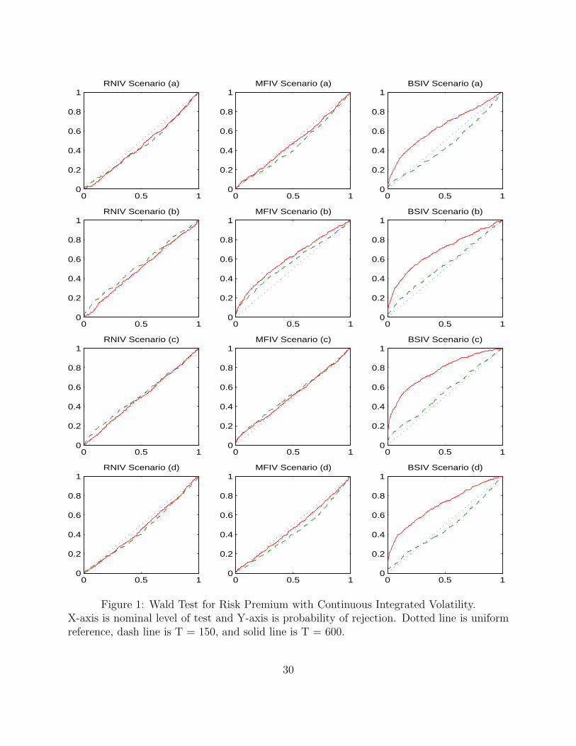
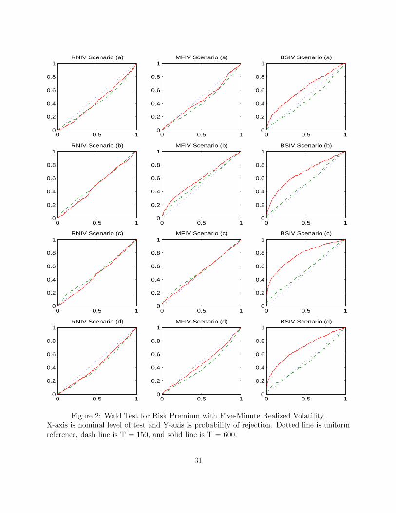
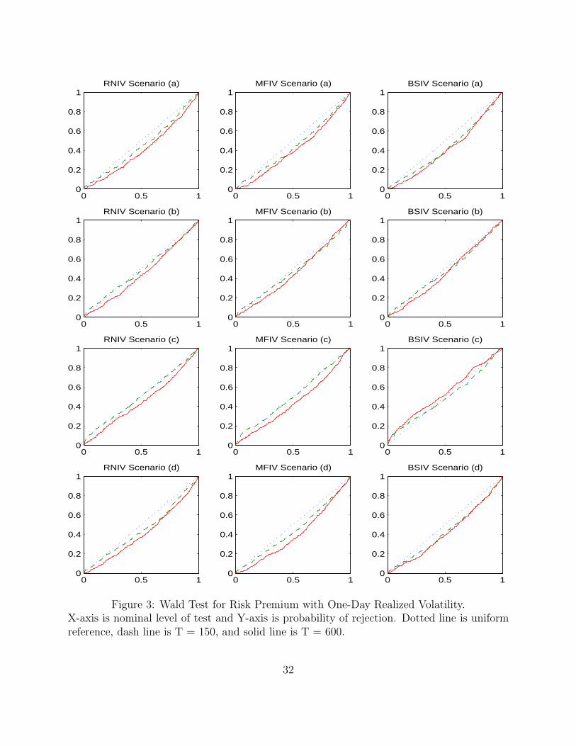
Figures 1-3 report the Wald test for the risk premium parameter, which should be asymp-

totically X 2(1) distributed. In the cases of (infeasible) integrated volatility and five-minute

realized volatility, the test statistics for the MFIV and RNIV measures are generally indis-

tinguishable and closely approximated by the asymptotic distribution, the only exception

being the high volatility persistence scenario (b) for which the MFIV measure results in

slight over-rejection. In contrast, the (misspecified) BSIV measure shows clear evidence of

over-rejection for all of the different scenarios. When the realized volatility is constructed

from daily squared returns, the Wald test systematically loses power to detect any misspeci-

fication, and the RNIV and MFIV measures now both show some under-rejection bias, while

the over-rejection bias for the BSIV measure is somewhat mitigated.9

In a sum, the Monte Carlo results clearly demonstrate the ability to accurately estimate

the volatility risk premium from the model-free implied volatilities along with the realized

volatilities from five-minute returns. On the other hand, the use of Black-Scholes implied

volatilities and/or realized volatilities from daily returns both produce biased and inefficient

estimates, and generally do not allow for reliable inference concerning the true value of the

risk premium parameter.

conditions for the model in (1) only.9The GMM omnibus test also has the correct size for the RNIV and MFIV measures, but often cannot

reject for the misspecified BSIV. This is because even for BSIV the objective moment (5) is still correctlyspecified, only the cross moment (8) is misspecified. These additional graphs are omitted to conserve spacebut available upon request.

10

4 Estimates for the Market Volatility Risk Premium

4.1 Data Sources and Summary Statistics

Our empirical analysis is based on monthly implied and realized volatilities for the S&P500

index from January 1990 through May 2004. For the risk-neutral implied volatility measure,

we rely on the VIX index provided by the Chicago Board of Options Exchange (CBOE). The

VIX index, available back to January 1990, is based on the liquid S&P500 index options,

and more importantly, it is calculated with the model-free approach in Britten-Jones and

Neuberger (2000).10 As shown in the Monte Carlo study, the model-free implied volatility

should be a good approximation to the true (unobserved) risk-neutral expectation of the

integrated volatility, and, in particular, a much better approximation than the one afforded

by the Black-Scholes implied volatility.

Our realized volatilities are based on the summation of the five-minute squared returns

on the S&P500 index within the month.11 Thus, for a typical month with 22 trading days,

we have 22×78 = 1, 716 five-minute returns, where the 78 five-minute subintervals cover the

normal trading hours from 9:30am to 4:00pm. Again, as indicated by the Monte Carlo sim-

ulations in the previous section, the monthly realized volatilities based on these five-minute

returns should provide a very good approximation to the true (unobserved) continuous-time

integrated volatility, and, in particular, a much better approximation than the one based on

daily squared returns.

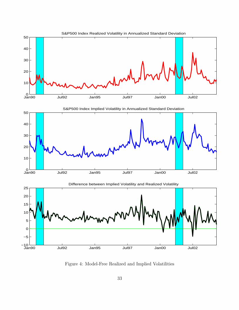
Figure 4 plots realized volatility, implied volatility, and their difference. (Here and

throughout the paper, monthly standard deviations are annualized by multiplying by√

12.)

It is clear that both volatility measures increased during the latter half of the sample, al-

though they have also both decreased more recently. Summary statistics for the two volatility

measures are reported in Table 4. Realized volatility is systematically lower than implied

volatility, and its unconditional distribution deviates more from the normal. Both measures

exhibit pronounced serial correlation with extremely slow decay in their autocorrelations,

suggestive long-memory type features.

There is a long history of market participants (and some academic researchers) using

the level of the VIX implied volatility as a gauge of market fear or, in the economists’

10In September 2003, CBOE replaced the old VIX index, based on S&P100 options and Black-Scholesimplied volatility, with the new VIX index based on S&P500 options and model-free implied volatility.Historical data on both the old and new VIX are directly available from the CBOE.

11The high-frequency data for the S&P500 index is provided by the Institute of Financial Markets.

11

jargon, investor risk aversion. Along similar lines, the difference between the implied and

realized volatilities have also been used as a benchmark for the market-implied risk aversion.

Unfortunately, the raw difference, as depicted in the bottom panel in Figure 4, is typically

very noisy and uninformative, and basically just trends with the level of volatility. A more

structured approach for extracting the volatility risk premium (or implied risk aversion), as

discussed in the previous sections, thus holds the promise of revealing a deeper understanding

of the way in which the volatility risk premium evolves over time, and its relationship to the

macroeconomy. We next turn to a discussion of our pertinent estimation results.

4.2 GMM Estimation of Time Varying Risk Premia

Table 5 reports the GMM estimation results for the three volatility risk premium specifica-

tions: (i) a constant λ; (ii) a time-varying λt+∆ driven by the error from the cross moment

as in equation (11); and (iii) a time-varying λt+∆ determined by the macro-finance variables

as in equation (12).12

First, restricting the risk premium to be constant results in a highly significant estimate

of -1.79. However, the chi-square omnibus test of overidentifying restrictions rejects the

overall specification at the 10% (although not at the 5%) level.

The second column of the table presents the result allowing for temporal variation in

the risk premium driven by the error from the cross moment. The corresponding estimated

coefficient (c = 0.02) is highly statistically significant. The estimates for this specification

also point toward a high degree of persistence (b = 0.80) in the volatility risk premium,

with an implied average value for the full sample of a/(1 − b) = −1.99. Yet, the overall

specification test continues to reject the model at the 10% (but not at the 5%) level.

To circumvent these shortcomings, the third column presents the results obtained by

explicitly including the macro-finance covariates. To select the macro-finance variables in

the time-varying risk premium specification, we did an extensive search with 29 monthly

data series (listed in Table 8). If part of the temporal variation in investor risk aversion

reflects investors focusing on different aspects of the economy at different points in time, as

seems likely, some flexibility in specifying the set of covariates seems both appropriate and

unavoidable. Hence, we select the group of variables that jointly achieves the highest p-

12In order to conserve space, we only report the results pertaining to the parameters for the volatilityrisk premium. The results for the other parameters in the model are directly in line with previous resultsreported in the literature, and consistent with the monthly summary statistics in Table 3, all point towarda high degree of volatility persistence in the (latent) Vt process.

12

value of the GMM omnibus specification test and that are significant (at the 5% level) based

on their individual t-test statistics.13 To facilitate the subsequent discussion, the resulting

seven variables have all been standardized to have mean zero and variance one so that their

marginal contribution to the time-varying risk premium are directly comparable.14

The results for the autoregressive part of the specification implies an average risk premium

of a/(1 − b) = −1.82, and, without figuring in the dynamic impact of the macro state

variables, an even higher degree of persistence, b = 0.93. As necessitated by the specification

search, all of the individual parameters for the macro-finance covariates are statistically

significant at the 5% level, and the overall GMM specification test is greatly improved, with

a p-value of 0.92. The resulting estimate for the volatility risk premium, along with the

seven macro-finance input variables, are plotted in Figure 5.

Both the signs and magnitudes of the macro-finance shock coefficients are important in

understanding the time-variation of the volatility risk premium. Sticking to the convention

that (−λ) represents the risk premium, or risk aversion, the realized volatility has the biggest

contribution (-0.32) and a positive impact (i.e., when volatility is high so is risk aversion).

The impact of AAA bond spread over Treasuries (0.19) likely reflects a business cycle effect

(i.e., credit spreads tend to be high before a downturn which usually coincides with low risk

aversion). Conversely, housing starts have a positive impact on the risk premium (-0.19) (i.e.,

a real estate boom usually precedes higher risk aversion). The S&P 500 P/E ratio is the

fourth most important factor (0.14), and impacts the premium negatively (i.e., everything

else equal, higher P/E ratios lowers the degree of risk aversion). The fifth variable in the

table is industrial production growth (0.10), which also has a negative impact (i.e., higher

growth leads to a lower volatility risk premium). On the contrary, the sixth CPI inflation

variable leads to higher risk aversion (-0.05). Finally, the last significant macro state variable,

payroll employment, marginally raises the volatility risk premium (-0.04), possibly as a result

of wage pressure.

13We are, of course, aware of the danger of data mining that such a specification search presents. However,we have attempted to limit the degree of data mining by choosing a limited set of candidate macro-financecovariates, listed in Table 8. Also, because our estimation relies on GMM, it is not necessarily the casethat adding more covariates always improves the fit of the model, as would be the case with linear OLSestimation.

14For stationary variables the unit is the level, while for non-stationary variables the unit is the logarithmicchange for the past twelve months.

13

4.3 Contrasting Strategies For Estimating A Time-Varying RiskPremium

Our approach for estimating the time-varying volatility risk premium can be contrasted

with other approaches in the literature for estimating time-varying risk premia. One such

approach is to vary the risk premium parameter each time period to best match that period’s

market data. In the context of volatility modeling, that approach would vary the risk

premium parameter to match each month’s difference between realized and implied volatility.

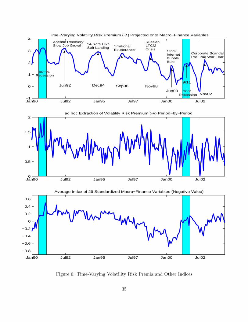
Such an approach would produce the time-varying risk premium shown in the middle panel

of Figure 6, the general shape of which matches the earlier plot in the bottom panel of Figure

4.

As previously noted, the problem with this approach is that by attributing each wiggle

in the data to changes in the risk premium, it produces an excessively volatile time series of

monthly risk premia. Economic theory argues that an asset’s risk premium should depend on

deep structural parameters. For example, in the consumption CAPM (C-CAPM), an asset’s

risk premium varies with investors’ risk aversion and the asset’s covariance with investors’

consumption. By definition, deep structural parameters should be relatively stable over

time. Yet the approach of period-by-period estimation of a time-varying risk premia forces

the parameters to vary (almost independently) from one period to the next. As such, we

find the monthly volatility risk premium series shown in the middle panel of Figure 6 to be

implausibly volatile.15

A second approach for estimating investors’ “risk appetite,” more popular among market

participants, is to construct a weighted-average of macro-finance variables.16 The bottom

panel of Figure 6 shows such a weighted-average index constructed from the macro-finance

variables listed in Table 8.17 In addition to concerns that such indexes are too ad hoc to be

reliable, indexes constructed in this way also tend to be excessively and implausibly volatile.

A third approach to estimating risk premium parameters comes from the macroeconomic,

or consumption-based asset pricing literature. This approach often assumes that risk premia

are constant, or if the premia are allowed to vary over time, they end up being implausibly

15Several recent papers have charts that look similar to the middle panel of Figure 6. For example, seeRosenberg and Engle (2002) page 363, Tarashev et al. (2003) page 62, and Bliss and Panigirtzoglou (2004)page 425.

16Chaboud (2003) discusses several such indexes constructed by J.P. Morgan, State Street Bank, andCredit Suisse First Boston.

17Following the practice in industry, the bottom panel of Figure 6 plots an average index (negative value)of 29 macro-finance variables that are standardized as mean zero and variance one.

14

smooth. For example, the estimated risk premium of Brandt and Wang (2003) does not even

pick out recessions, except for the 1978-82 monetary experiment period.

A fourth strand of the literature focuses on models in which the risk premium are modeled

as varying over longer-run business cycle frequencies. For example, Campbell and Cochrane

(1999) generate time variation in risk aversion through habit formation in which the level of

habit reacts only gradually to changes in consumption. Such a modeling strategy explicitly

prevents the risk premia from being excessively variable in the short-run. In a similar vein,

Cochrane and Piazzesi (2004) model a slowly varying risk premia on Treasury bonds as a

function of current forward rates.

Our method and results fall squarely within this fourth strand of the literature. The

top panel of Figure 6 plots our estimated volatility risk premium parameter based on the

model involving the seven macro-finance covariates. Peaks and troughs in the series are

generally multiple years apart, and reassuringly the series is void of the excessive month-

by-month fluctuations that plague both of the other two series in the figure. The estimated

risk premium also rises sharply during the two NBER-dated macroeconomic recessions (the

shaded areas in the plots), as well as the periods of slow recovery and job growth after

the 1991 and 2001 recessions. Moreover, the peaks in the series are readily identifiable with

major macroeconomic or financial market developments, including the 1994 rate hike and soft

landing, the 1998 Russian debt crisis, and the bursting of the stock market “bubble” in 2000.

There is also a peak in the risk premium in 1996 that does not appear to directly line up with

any major economic or financial event, except perhaps the worry about over-valuation in the

stock market sometimes labeled as the period of “Irrational Exuberance”. Interestingly, the

estimates also suggest that the risk premium rises fairly sharply but declines only gradually.

4.4 Risk Premium Variation and Stock Return Predictability

Our characterization of the volatility risk premium has the potential of being informative

about other risk premia in the economy. To illustrate, we compare its predictive power for

aggregate stock market returns with that of other traditionally-used macro-finance variables.

To that end, the top panel of Table 6 reports the results of simple univariate regressions of

the monthly S&P500 excess returns on the most significant individual variables from the

pool of covariates listed in Table 8. As evidenced by the results, the extracted volatility risk

15

premium has the highest predictive power with an R2 of 3.67%.18 The next best predictor

is the S&P500 P/E ratio with an R2 of 2.80%. Next in order are industrial production and

nonfarm payrolls with R2’s of 1.53% and 1.06%, respectively. Dividend yields - a significant

predictor according to many other studies - only explains 0.85% of the monthly return

variation. All-in-all, these results are consistent with previous findings that macroeconomic

state variables do predict returns, though the predictability measured by R2 is usually in

the low single digits. Nonetheless, it is noteworthy that of all the predictor variables, the

volatility risk premium results in the single highest R2.

Combining all of the marginally significant variables into a single multiple regression,

results in the estimates shown in the bottom panel of Table 6. Interestingly, none of the

macro-finance variable remains significant when the volatility risk premium is included, while

only the P/E ratio is significant in the regression excluding the premium. Of course, the

estimate for the volatility risk premium already incorporates some of the same macroeco-

nomic variables (see Table 5), so the finding that these variables are “driven out” when

included together with the premium is not necessarily that surprising. However, the macro

variables entering the model for λt+∆ only impact the returns indirectly through the tempo-

ral variation in the premium, and the volatility risk premium itself is also estimated from a

very different set of moment conditions based on the model-free realized and options implied

volatilities.

Our examination of the monthly stock excess return in Table 6 singles out the volatility

risk premium (which we interpret as a proxy for risk aversion) and the stock market PE ratio

(which we interpret as a proxy for fundamental risk) as the two most important predictor

variables. Table 7 augments these results with regressions involving longer-run quarterly

excess returns spanning 1990Q1 through 2003Q2. In addition to the volatility risk premium

and the PE ratio from the last month of the previous quarter, we also include the quarterly

consumption-wealth ratio in these regressions. The consumption-wealth ratio, termed CAY,

has previously been established by (Lettau and Ludvigson, 2001) as an important explana-

tory variable for longer horizon returns. The first three regressions in the table show that

each of the three variables is indeed individually significant. At the same time, it is notewor-

thy that the risk premium results in the highest individual R2 of 11.6%, much higher than

the monthly R2 of 3.7%. Adding the P/E ratio and/or the CAY variable further increase the

18The use of the volatility risk premium as a second-stage regressor suffers from a standard errors-in-variables type problem, resulting in too large a standard error for the estimated slope coefficient.

16

quarterly R2’s in excess of 14%. The risk premium remains significant in all of the multiple

regressions, while combining the P/E ratio and the CAY variable in the same regression

renders both insignificant, and does not increase the R2 by much. As such, these results

further reinforce the earlier findings for the monthly returns in Table 6 and the role of the

estimated volatility risk premium as a new and powerful stock market predictor over longer

quarterly horizons.

5 Conclusion

This paper develops a simple consistent approach for estimating the volatility risk premium.

The approach exploits the linkage between the objective and risk-neutral expectations of the

integrated volatility. The estimation is facilitated by the use of newly available model-free

realized volatilities based on high-frequency intraday data along with model-free option-

implied volatilities. The approach allows us to explicitly link any temporal variation in the

risk premium to underlying state variables within an internally consistent and simple-to-

implement GMM estimation framework.

A small scale Monte Carlo experiment indicates that the procedure performs well in

estimating the volatility risk premium in empirically realistic situations. In contrast, the

estimates based on the Black-Scholes implied volatilities and/or monthly sample variances

based on daily squared returns result in highly inefficient and statistically unreliable esti-

mates of the risk premium. Applying the methodology to the S&P500 market index, we

find significant evidence for temporal variation in the volatility risk premium, which we di-

rectly link to a set of underlying macro-finance state variables. The extracted volatility risk

premium is also found to be helpful in predicting the return on the market itself.

The volatility risk premium (or risk aversion) extracted in our paper differs sharply

from other approaches in the literature. In particular, earlier estimates relying directly on

period-by-period differences in the estimated risk-neutral and objective distributions tend

to produce implausibly volatile estimates. On the other hand, earlier procedures based on

structural macroeconomic/consumption-type pricing models typically result in implausibly

smooth estimates. In contrast, the model-free realized and implied volatility-based procedure

developed here results in a volatility risk premium (or risk aversion index) that avoids the

excessive period-by-period random fluctuations yet responds to recessions, financial crises,

and other economic events in an empirically realistic fashion.

17

It would be interesting to more closely compare and contrast the risk aversion index esti-

mated here to other popular gauges of investor fear or market sentiment. Along these lines,

it would also be interesting to explore the evidence from other markets, both domestically

and internationally. How do the estimated risk premia correlate across different markets and

countries? The results in the paper for the S&P500 indicate that the volatility risk premium

for the current month is useful in predicting the next month’s return. Again, what about

other markets? Does the estimated risk aversion index for the aggregate stock market help

in predicting bond market premia? Better estimates of the volatility risk premium could

also result in more accurate prices for derivatives. We leave further work along these lines

for future research.

18

References

Aıt-Sahalia, Yacine, Yubo Wang, and Francis Yared (2001), “Do Option Markets Correctly

Price the Probabilities of Movement of the Underlying Asset?” Journal of Econometrics,

vol. 102, 67–110.

Andersen, Torben G., Tim Bollerslev, and Francis X. Diebold (2003a), Handbook of Finan-

cial Econometrics , chap. Parametric and Nonparametric Volatility Measurement, Elsevier

Science B.V., Amsterdam, forthcoming.

Andersen, Torben G., Tim Bollerslev, Francis X. Diebold, and Heiko Ebens (2001), “The

Distribution of Realized Stock Return Volatility,” Journal of Financial Economics , vol. 61,

43–76.

Andersen, Torben G., Tim Bollerslev, Francis X. Diebold, and Paul Labys (2003b), “Mod-

eling and Forecasting Realized Volatility,” Econometrica, vol. 71, 579–625.

Andersen, Torben G., Tim Bollerslev, and Nour Meddahi (2004), “Analytical Evaluation of

Volatility Forecasts,” International Economic Review , forthcoming.

Bakshi, Gurdip and Nikunj Kapadia (2003), “Delta-Hedged Gains and the Negative Market

Volatility Risk Premium,” Review of Financial Studies, vol. 16, 527–566.

Barndorff-Nielsen, Ole and Neil Shephard (2002), “Econometric Analysis of Realised Volatil-

ity and Its Use in Estimating Stochastic Volatility Models,” Journal of Royal Statistical

Society , vol. Series B 64.

Barndorff-Nielsen, Ole and Neil Shephard (2004a), “Econometric Analysis of Realised Co-

variation: High Frequency Based Covariance, Regression and Correlation,” Econometrica,

vol. 72, 885–925.

Barndorff-Nielsen, Ole and Neil Shephard (2004b), “A Feasible Central Limit Theory for

Realised Volatility under Leverage,” manuscript , Nuffield College, Oxford University.

Bates, David S. (1996), “Jumps and Stochastic Volatility: Exchange Rate Process Implicit

in Deutsche Mark Options,” The Review of Financial Studies, vol. 9, 69–107.

Benzoni, Luca (2001), “Pricing Options under Stochastic Volatility: An Empirical Investi-

gation,” Working Paper , University of Minnesota.

19

Bliss, Robert R. and Nikolaos Panigirtzoglou (2004), “Option-Implied Risk Aversion Esti-

mates,” Journal of Finance, vol. 59, 407 – 446.

Bollerslev, Tim and Hao Zhou (2002), “Estimating Stochastic Volatility Diffusion Using

Conditional Moments of Integrated Volatility,” Journal of Econometrics, vol. 109, 33–65.

Bollerslev, Tim and Hao Zhou (2004), “Volatility Puzzles: A Simple Framework for Gaug-

ing Return-Volatility Regressions,” Working Paper , Duke University and Federal Reserve

Board.

Brandt, Michael W. and Kevin Q. Wang (2003), “Time-varying Risk Aversion and Expected

Inflation,” Journal of Monetary Economics , vol. 50, 1457–1498.

Britten-Jones, Mark and Anthony Neuberger (2000), “Option Prices, Implied Price Pro-

cesses, and Stochastic Volatility,” Journal of Finance, vol. 55, 839–866.

Campbell, John Y. (1987), “Stock Returns and the Term Structure,” Journal of Financial

Economics , vol. 18, 373–399.

Campbell, John Y. and John H. Cochrane (1999), “By Force of Habit: A Consumption

Based Explanation of Aggregate Stock Market Behavior,” Journal of Political Economy ,

vol. 107, 205–251.

Campbell, John Y. and Robert J. Shiller (1988a), “The Dividend-Price Ratio and Expec-

tations of Future Dividends and Discount Factors,” Review of Financial Studies, vol. 1,

195–228.

Campbell, John Y. and Robert J. Shiller (1988b), “Stock Prices, Earnings, and Expected

Dividends,” Journal of Finance, vol. 43, 661–676.

Chaboud, Alain (2003), “Indexes of Risk Appetite in International Financial Markets,”

mimeo, Federal Reserve Board.

Chernov, Mikhail and Eric Ghysels (2000), “A Study towards a Unified Approach to the

Joint Estimation of Objective and Risk Neutral Measures for the Purpose of Options

Valuation,” Journal of Financial Economics , vol. 56, 407–458.

Cochrane, John H. and Monika Piazzesi (2004), “Bond Risk Premia,” NBER Working Paper

9178 .

20

Demeterfi, Kresimir, Emanuel Derman, Michael Kamal, and Joseph Zou (1999), “A Guide

to Volatility and Variance Swaps,” Journal of Derivatives , vol. 6, 1–1.

Eraker, Bjørn (2004), “Do Stock Prices and Volatility Jump? Reconciling Evidence from

Spot and Option Prices,” Journal of Finance, vol. 59, 1367–1403.

Fama, Eugene F. and Robert R. Bliss (1987), “The information in Long-Maturity Forward

Rates,” The American Economic Review , vol. 77, 680–692.

Fama, Eugene F. and Kenneth R. French (1988), “Dividend Yields and Expected Stock

Returns,” Journal of Financial Economics , vol. 22, 3–25.

Garcia, Rene, Marc-Andre Lewis, and Eric Renault (2001), “Estimation of Objective and

Risk-Neutral Distributions Based on Moments of Integrated Volatility,” Working Paper ,

CRDE, Universite de Montreal.

Hansen, Lars Peter (1982), “Large Sample Properties of Generalized Method of Moments

Estimators,” Econometrica, vol. 50, 1029–1054.

Heston, Steven (1993), “A Closed-Form Solution for Options with Stochastic Volatility with

Applications to Bond and Currency Options,” Review of Financial Studies, vol. 6, 327–

343.

Jiang, George and Yisong Tian (2004), “Model-Free Implied Volatility and Its Information

Content,” Review of Financial Studies, forthcoming.

Lettau, Martin and Sydney Ludvigson (2001), “Consumption, Aggregate Wealth, and Ex-

pected Stock Returns,” Journal of Finance, vol. 56, 815–849.

Lynch, Damien and Nikolaos Panigirtzoglou (2003), “Option Implied and Realized Mea-

sures of Variance,” Working Paper , Monetary Instruments and Markets Division, Bank of

England.

Meddahi, Nour (2002), “Theoretical Comparison Between Integrated and Realized Volatil-

ity,” Journal of Applied Econometrics , vol. 17, 479–508.

Newey, Whitney K. and Kenneth D. West (1987), “A Simple Positive Semi-Definite,

Heteroskedasticity and Autocorrelation Consistent Covariance Matrix,” Econometrica,

vol. 55, 703–708.

21

Pan, Jun (2002), “The Jump-Risk Premia Implicit in Options: Evidence from an Integrated

Time-Series Study,” Journal of Financial Economics , vol. 63, 3–50.

Rosenberg, Joshua V. and Robert F. Engle (2002), “Empirical Pricing Kernels,” Journal of

Financial Economics, vol. 64, 341–372.

Tarashev, Nikola, Kostas Tsatsaronis, and Dimitrios Karampatos (2003), “Investors’ Atti-

tude toward Risk: What Can We Learn from Options?” BIS Quarterly Review , Bank of

International Settlement.

22

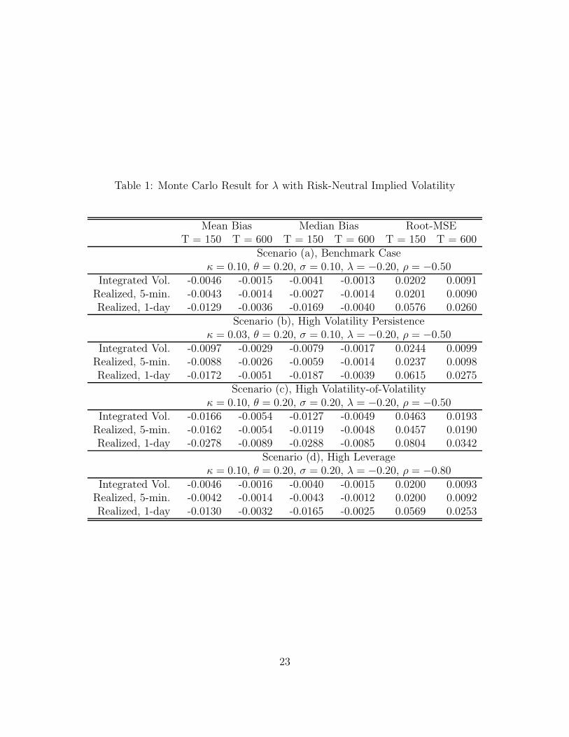
Table 1: Monte Carlo Result for λ with Risk-Neutral Implied Volatility

Mean Bias Median Bias Root-MSET = 150 T = 600 T = 150 T = 600 T = 150 T = 600

Scenario (a), Benchmark Caseκ = 0.10, θ = 0.20, σ = 0.10, λ = −0.20, ρ = −0.50

Integrated Vol. -0.0046 -0.0015 -0.0041 -0.0013 0.0202 0.0091Realized, 5-min. -0.0043 -0.0014 -0.0027 -0.0014 0.0201 0.0090Realized, 1-day -0.0129 -0.0036 -0.0169 -0.0040 0.0576 0.0260

Scenario (b), High Volatility Persistenceκ = 0.03, θ = 0.20, σ = 0.10, λ = −0.20, ρ = −0.50


Scenario (c), High Volatility-of-Volatilityκ = 0.10, θ = 0.20, σ = 0.20, λ = −0.20, ρ = −0.50


Scenario (d), High Leverageκ = 0.10, θ = 0.20, σ = 0.20, λ = −0.20, ρ = −0.80


23

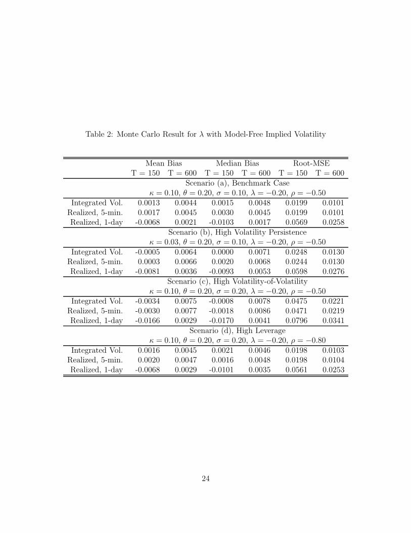
Table 2: Monte Carlo Result for λ with Model-Free Implied Volatility



Integrated Vol. 0.0013 0.0044 0.0015 0.0048 0.0199 0.0101Realized, 5-min. 0.0017 0.0045 0.0030 0.0045 0.0199 0.0101Realized, 1-day -0.0068 0.0021 -0.0103 0.0017 0.0569 0.0258


Integrated Vol. -0.0005 0.0064 0.0000 0.0071 0.0248 0.0130Realized, 5-min. 0.0003 0.0066 0.0020 0.0068 0.0244 0.0130Realized, 1-day -0.0081 0.0036 -0.0093 0.0053 0.0598 0.0276


Integrated Vol. -0.0034 0.0075 -0.0008 0.0078 0.0475 0.0221Realized, 5-min. -0.0030 0.0077 -0.0018 0.0086 0.0471 0.0219Realized, 1-day -0.0166 0.0029 -0.0170 0.0041 0.0796 0.0341



24

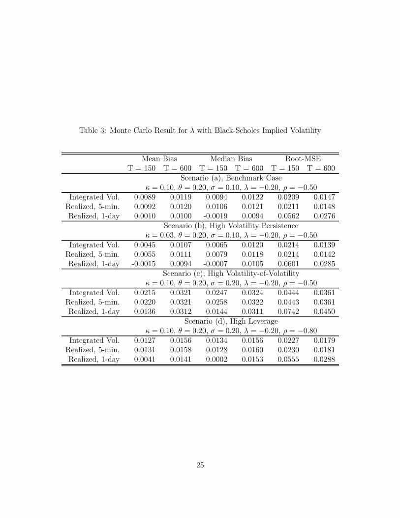
Table 3: Monte Carlo Result for λ with Black-Scholes Implied Volatility



Integrated Vol. 0.0089 0.0119 0.0094 0.0122 0.0209 0.0147Realized, 5-min. 0.0092 0.0120 0.0106 0.0121 0.0211 0.0148Realized, 1-day 0.0010 0.0100 -0.0019 0.0094 0.0562 0.0276




Integrated Vol. 0.0215 0.0321 0.0247 0.0324 0.0444 0.0361Realized, 5-min. 0.0220 0.0321 0.0258 0.0322 0.0443 0.0361Realized, 1-day 0.0136 0.0312 0.0144 0.0311 0.0742 0.0450


Integrated Vol. 0.0127 0.0156 0.0134 0.0156 0.0227 0.0179Realized, 5-min. 0.0131 0.0158 0.0128 0.0160 0.0230 0.0181Realized, 1-day 0.0041 0.0141 0.0002 0.0153 0.0555 0.0288

25

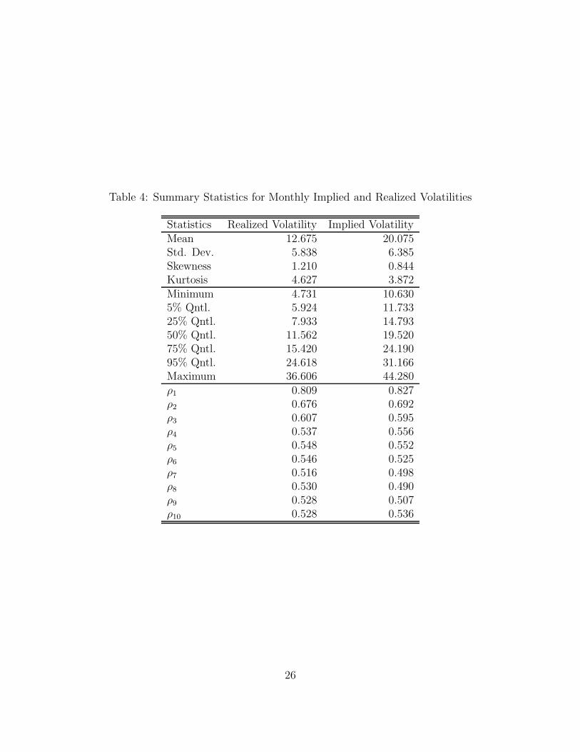
Table 4: Summary Statistics for Monthly Implied and Realized Volatilities

Statistics Realized Volatility Implied VolatilityMean 12.675 20.075Std. Dev. 5.838 6.385Skewness 1.210 0.844Kurtosis 4.627 3.872Minimum 4.731 10.6305% Qntl. 5.924 11.73325% Qntl. 7.933 14.79350% Qntl. 11.562 19.52075% Qntl. 15.420 24.19095% Qntl. 24.618 31.166Maximum 36.606 44.280ρ1 0.809 0.827ρ2 0.676 0.692ρ3 0.607 0.595ρ4 0.537 0.556ρ5 0.548 0.552ρ6 0.546 0.525ρ7 0.516 0.498ρ8 0.530 0.490ρ9 0.528 0.507ρ10 0.528 0.536

26

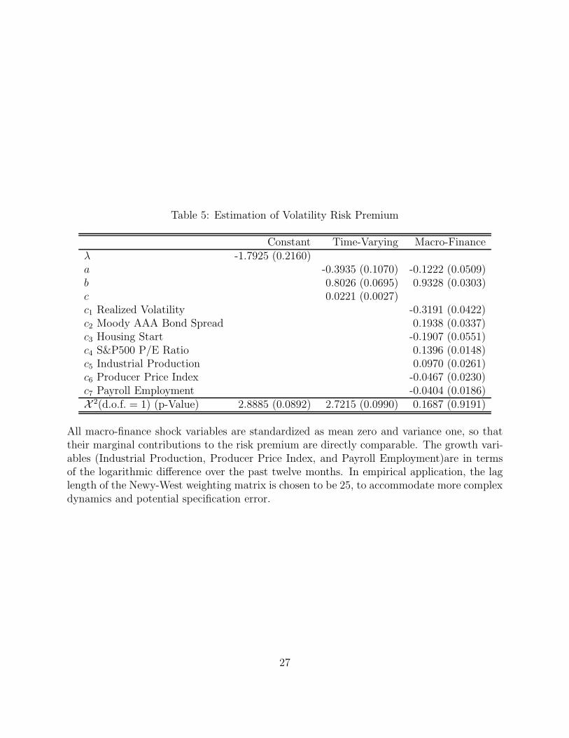
Table 5: Estimation of Volatility Risk Premium

Constant Time-Varying Macro-Financeλ -1.7925 (0.2160)a -0.3935 (0.1070) -0.1222 (0.0509)b 0.8026 (0.0695) 0.9328 (0.0303)c 0.0221 (0.0027)c1 Realized Volatility -0.3191 (0.0422)c2 Moody AAA Bond Spread 0.1938 (0.0337)c3 Housing Start -0.1907 (0.0551)c4 S&P500 P/E Ratio 0.1396 (0.0148)c5 Industrial Production 0.0970 (0.0261)c6 Producer Price Index -0.0467 (0.0230)c7 Payroll Employment -0.0404 (0.0186)X 2(d.o.f. = 1) (p-Value) 2.8885 (0.0892) 2.7215 (0.0990) 0.1687 (0.9191)

All macro-finance shock variables are standardized as mean zero and variance one, so thattheir marginal contributions to the risk premium are directly comparable. The growth vari-ables (Industrial Production, Producer Price Index, and Payroll Employment)are in termsof the logarithmic difference over the past twelve months. In empirical application, the laglength of the Newy-West weighting matrix is chosen to be 25, to accommodate more complexdynamics and potential specification error.

27

Table 6: Monthly Stock Market Return Predictability

Variables Intercept (s.e.) Slope (s.e.) R-SquareVolatility Risk Premium -18.5125 (10.5826) 12.4880 (5.1847) 0.0367S&P500 PE Ratio 35.9389 (13.7503) -1.2719 (0.5658) 0.0280Industrial Production -0.9257 ( 5.4952) 1.9922 (1.2255) 0.0153Nonfarm Payroll Employment -0.3110 ( 5.4777) 3.6432 (2.6236) 0.010626 Other Macro-Finance Variables <0.0100

Joint Estimation Including λt Excluding λt

Variables Parameter (s.e.) Parameter (s.e.)Intercept 3.5760 (20.2995) 32.6190 (15.3063)Volatility Risk Premium 8.3377 ( 5.4925)S&P500 PE Ratio -0.7055 ( 0.5684) -1.2592 ( 0.5854)Industrial Production 2.0651 ( 2.2621) 2.7192 ( 2.2043)Nonfarm Payroll Employment -1.9441 ( 4.6999) -3.3062 ( 4.6570)R-Square 0.0502 0.0389

The table reports the predictive regressions for the monthly excess return of S&P500 indexmeasured in annualized percentage term. Industrial Production and Payroll Employmentnumbers are the past year logarithmic changes in annualized percentages.

Table 7: Quarterly Stock Market Return Predictability

Intercept (s.e.) Risk Premium (s.e.) PE Ratio (s.e.) CAY (s.e.) R-Square-22.0391 (12.8401) 13.6314 (6.2762) 0.116341.0442 (16.2894) -1.5429 (0.6923) 0.10342.4129 ( 4.3077) 5.3777 (2.0306) 0.08548.7403 (17.5761) 9.5126 (5.4502) -0.9460 (0.5894) 0.1445

-16.7554 (13.5454) 10.4940 (6.8287) 3.1917 (1.7862) 0.140229.7368 (27.8876) -1.0978 (1.1394) 2.4763 (3.3519) 0.11292.4033 (23.7001) 9.0313 (5.6439) -0.6624 (0.9622) 1.7457 (3.0405) 0.1491

To be comparable, our data set is transformed into quarterly frequency, dating from 1990Q1to 2003Q2. “CAY” stands for the consumption wealth ratio as in Lettau and Ludvigson(2001), and the data is downloaded from their website.

28

Table 8: List of Macro-Finance Variables

Macro-Finance Variables Data SourceS&P500 Realized Volatility Constructed from IFM (CME)S&P500 Implied Volatility CBOES&P500 Market Return Standard & PoorsS&P500 PE Ratio Standard & PoorsS&P500 Dividend Yield Standard & PoorsNYSE Trading Volume NYSEUnemployment Rate Bureau of Labor StatisticsNonfarm Payroll Employment Bureau of Labor StatisticsIndustrial Capacity Utilization Federal ReserveIndustrial Production Federal ReserveCPI Inflation Bureau of Labor StatisticsProducer Price Index Bureau of Labor StatisticsExpected CPI Inflation Michigan SurveyTreasury Spread 5yr-6mn Federal ReserveTreasury Spread 10yr-6mn Federal ReserveMortgage Spread (over 10yr Treasury) Federal ReserveSwap Spread (over 10yr Treasury) BloombergAAA Corporate Spread (over 10yr Treasury) MoodyBAA Corporate Spread (over 10yr Treasury) MoodyAA Corporate Spread (over 10yr Treasury) Merrill LynchBBB Corporate Spread (over 10yr Treasury) Merrill LynchConsumer Sentiment Michigan SurveyConsumer Sentiment (Expected) Michigan SurveyConsumer Confidence Conference BoardConsumer Confidence (Expected) Conference BoardHousing Permit Number HUDHousing Start Number HUDMoney Supply (M2) Federal ReserveBusiness Cycle Indicator NBER

29

0 0.5 10

0.2

0.4

0.6

0.8

1RNIV Scenario (a)

0 0.5 10

0.2

0.4

0.6

0.8

1MFIV Scenario (a)

0 0.5 10

0.2

0.4

0.6

0.8

1BSIV Scenario (a)

0 0.5 10

0.2

0.4

0.6

0.8

1RNIV Scenario (b)

0 0.5 10

0.2

0.4

0.6

0.8

1MFIV Scenario (b)

0 0.5 10

0.2

0.4

0.6

0.8

1BSIV Scenario (b)

0 0.5 10

0.2

0.4

0.6

0.8

1RNIV Scenario (c)

0 0.5 10

0.2

0.4

0.6

0.8

1MFIV Scenario (c)

0 0.5 10

0.2

0.4

0.6

0.8

1BSIV Scenario (c)

0 0.5 10

0.2

0.4

0.6

0.8

1RNIV Scenario (d)

0 0.5 10

0.2

0.4

0.6

0.8

1MFIV Scenario (d)

0 0.5 10

0.2

0.4

0.6

0.8

1BSIV Scenario (d)

Figure 1: Wald Test for Risk Premium with Continuous Integrated Volatility.X-axis is nominal level of test and Y-axis is probability of rejection. Dotted line is uniformreference, dash line is T = 150, and solid line is T = 600.

30

0 0.5 10

0.2

0.4

0.6

0.8

1RNIV Scenario (a)

0 0.5 10

0.2

0.4

0.6

0.8

1MFIV Scenario (a)

0 0.5 10

0.2

0.4

0.6

0.8

1BSIV Scenario (a)

0 0.5 10

0.2

0.4

0.6

0.8

1RNIV Scenario (b)

0 0.5 10

0.2

0.4

0.6

0.8

1MFIV Scenario (b)

0 0.5 10

0.2

0.4

0.6

0.8

1BSIV Scenario (b)

0 0.5 10

0.2

0.4

0.6

0.8

1RNIV Scenario (c)

0 0.5 10

0.2

0.4

0.6

0.8

1MFIV Scenario (c)

0 0.5 10

0.2

0.4

0.6

0.8

1BSIV Scenario (c)

0 0.5 10

0.2

0.4

0.6

0.8

1RNIV Scenario (d)

0 0.5 10

0.2

0.4

0.6

0.8

1MFIV Scenario (d)

0 0.5 10

0.2

0.4

0.6

0.8

1BSIV Scenario (d)

Figure 2: Wald Test for Risk Premium with Five-Minute Realized Volatility.X-axis is nominal level of test and Y-axis is probability of rejection. Dotted line is uniformreference, dash line is T = 150, and solid line is T = 600.

31

0 0.5 10

0.2

0.4

0.6

0.8

1RNIV Scenario (a)

0 0.5 10

0.2

0.4

0.6

0.8

1MFIV Scenario (a)

0 0.5 10

0.2

0.4

0.6

0.8

1BSIV Scenario (a)

0 0.5 10

0.2

0.4

0.6

0.8

1RNIV Scenario (b)

0 0.5 10

0.2

0.4

0.6

0.8

1MFIV Scenario (b)

0 0.5 10

0.2

0.4

0.6

0.8

1BSIV Scenario (b)

0 0.5 10

0.2

0.4

0.6

0.8

1RNIV Scenario (c)

0 0.5 10

0.2

0.4

0.6

0.8

1MFIV Scenario (c)

0 0.5 10

0.2

0.4

0.6

0.8

1BSIV Scenario (c)

0 0.5 10

0.2

0.4

0.6

0.8

1RNIV Scenario (d)

0 0.5 10

0.2

0.4

0.6

0.8

1MFIV Scenario (d)

0 0.5 10

0.2

0.4

0.6

0.8

1BSIV Scenario (d)

Figure 3: Wald Test for Risk Premium with One-Day Realized Volatility.X-axis is nominal level of test and Y-axis is probability of rejection. Dotted line is uniformreference, dash line is T = 150, and solid line is T = 600.

32

Jan90 Jul92 Jan95 Jul97 Jan00 Jul020

10

20

30

40

50S&P500 Index Realized Volatility in Annualized Standard Deviation


10

20

30

40

50S&P500 Index Implied Volatility in Annualized Standard Deviation

Jan90 Jul92 Jan95 Jul97 Jan00 Jul02−10

−5

0

5

10

15

20

25Difference between Implied Volatility and Realized Volatility

Figure 4: Model-Free Realized and Implied Volatilities

33

Jan90 Jan95 Jan00

0

1

2

3

Volatility Risk Premium

Jan90 Jan95 Jan00

0

2

4

6

Realized Volatility

Jan90 Jan95 Jan00−2

−1

0

1

2

3

Moody AAA Bond Spread


−4

−2

0

2

New House Start Number


−1

0

1

2

3

S&P500 PE Ratio


−2

−1

0

1

2Industrial Production

Jan90 Jan95 Jan00

−2

−1

0

1

2

3Producer Price Index

Jan90 Jan95 Jan00

−2

−1

0

1

Nonfarm Payroll Employment

Figure 5: Macro-Finance Inputs for Volatility Risk Premium

34

Jan90 Jul92 Jan95 Jul97 Jan00 Jul02−1

0

1

2

3

4Time−Varying Volatility Risk Premium (−λ) Projected onto Macro−Finance Variables


0.5

1

1.5

2ad hoc Extraction of Volatility Risk Premium (−λ) Period−by−Period


−0.8

−0.6

−0.4

−0.2

0

0.2

0.4

0.6

Average Index of 29 Standardized Macro−Finance Variables (Negative Value)

Jun92 Dec94

94 Rate Hike Soft Landing

Sep96

"Irrational Exuberance"

Nov98

RussianLTCM Crisis

Jun00

Stock InternetBubble Bust

9/11

Nov02

Corporate Scandal Pre−Iraq War Fear

2001 Recession

90−91 Recession

Anemic Recovery Slow Job Growth

Figure 6: Time-Varying Volatility Risk Premia and Other Indices

35

Dynamic Estimation of Volatility Risk Premia and Investor Risk ...

Documents

Transcript of Dynamic Estimation of Volatility Risk Premia and Investor Risk ...