
DYNAMIC EFFECTS OF IDIOSYNCRATIC VOLATILITY...
58
1 DYNAMIC EFFECTS OF IDIOSYNCRATIC VOLATILITY AND LIQUIDITY ON CORPORATE BOND SPREADS Madhu Kalimipalli* Associate Professor School of Business & Economics Wilfrid Laurier University Waterloo, Canada, N2L 3C5 (519)-884-0710 (ext: 2187) [email protected] Subhankar Nayak Associate Professor School of Business & Economics Wilfrid Laurier University Waterloo, Canada, N2L 3C5 (519)-884-0710 (ext: 2206) [email protected] M. Fabricio Perez Assistant Professor School of Business & Economics Wilfrid Laurier University Waterloo, Canada, N2L 3C5 (519)-884-0710 (ext: 2532) [email protected] Abstract We study the dynamic impact of idiosyncratic volatility and bond liquidity on corporate bond spreads over time and empirically disentangle both effects. Using an extensive data set, we find that both idiosyncratic volatility and liquidity are critical mainly for the distress portfolios, i.e., low-rated and short-term bonds; for others only volatility matters. The effects of volatility and liquidity shocks on bond spreads were both exacerbated during the recent financial crisis. Liquidity shocks are quickly absorbed into bonds prices; however, volatility shocks are more persistent and have a long-term effect. Our results overall suggest significant differences between how volatility and liquidity dynamically impact bond spreads. Key Words: bond liquidity, equity volatility, corporate bond spreads, dynamic relationships JEL Classification: G10, G14 (Draft: January 31, 2013) * Kalimipalli is the corresponding author. The authors thank Sanjiv Das, Gady Jacoby, and participants at the NFA (Winnipeg) Annual Conference 2010, EFA (Savannah) Annual Conference 2011, CIGI (Waterloo) Econometrics Conference 2011, and FMA (Denver) Annual Conference 2011. This research is supported by the Social Sciences and Humanities Research Council of Canada.
Transcript of DYNAMIC EFFECTS OF IDIOSYNCRATIC VOLATILITY...

1
DYNAMIC EFFECTS OF IDIOSYNCRATIC VOLATILITY AND LIQUIDITY ON CORPORATE BOND SPREADS
Madhu Kalimipalli* Associate Professor
School of Business & Economics Wilfrid Laurier University
Waterloo, Canada, N2L 3C5 (519)-884-0710 (ext: 2187)
Subhankar Nayak Associate Professor
School of Business & Economics Wilfrid Laurier University
Waterloo, Canada, N2L 3C5 (519)-884-0710 (ext: 2206)
M. Fabricio Perez Assistant Professor
School of Business & Economics Wilfrid Laurier University
Waterloo, Canada, N2L 3C5 (519)-884-0710 (ext: 2532)
Abstract
We study the dynamic impact of idiosyncratic volatility and bond liquidity on corporate bond spreads over time and empirically disentangle both effects. Using an extensive data set, we find that both idiosyncratic volatility and liquidity are critical mainly for the distress portfolios, i.e., low-rated and short-term bonds; for others only volatility matters. The effects of volatility and liquidity shocks on bond spreads were both exacerbated during the recent financial crisis. Liquidity shocks are quickly absorbed into bonds prices; however, volatility shocks are more persistent and have a long-term effect. Our results overall suggest significant differences between how volatility and liquidity dynamically impact bond spreads.
Key Words: bond liquidity, equity volatility, corporate bond spreads, dynamic relationships JEL Classification: G10, G14
(Draft: January 31, 2013)
* Kalimipalli is the corresponding author. The authors thank Sanjiv Das, Gady Jacoby, and participants at the NFA (Winnipeg) Annual Conference 2010, EFA (Savannah) Annual Conference 2011, CIGI (Waterloo) Econometrics Conference 2011, and FMA (Denver) Annual Conference 2011. This research is supported by the Social Sciences and Humanities Research Council of Canada.

2
DYNAMIC EFFECTS OF IDIOSYNCRATIC VOLATILITY AND LIQUIDITY ON CORPORATE BOND SPREADS
1. INTRODUCTION
Does idiosyncratic risk contain information about liquidity in explaining the time-
series of corporate bond prices? We examine this question by studying the relative
importance of idiosyncratic volatility and liquidity for corporate bond yield spreads over time
and empirically disentangling both effects.
Idiosyncratic equity volatility (idiosyncratic volatility, hereafter) can be defined as
the residual firm volatility after controlling for systematic market risk factors. Theoretically,
an increase in idiosyncratic volatility, following a lower stock price, leads to lower
“distance-to-default” or higher default intensity of a firm and hence higher ex-ante bond
spreads (Merton, 19741
Motivated by the fact that the secondary market for corporate debt remains highly
illiquid (e.g., Henderson et al., 2006; Edwards and Piwowar, 2007), several studies find that
incorporating non-default sources of risk such as illiquidity can help address pricing biases in
the structural models and explain the “credit puzzle” (e.g., Huang and Huang, 2003;
Driessen, 2005; and Covitz and Downing, 2007).
; Das and Sundaram, 2007). This theoretical result is empirically
confirmed by Campbell and Taksler (2003), who find that idiosyncratic volatility is a
significant driver of bond spreads, after controlling for several bond characteristics.
2
In this paper, we explore the differential effects of idiosyncratic volatility and
liquidity on bond spread changes over time and study their dynamic relationships. While
most previous papers exclusively focus on either volatility or liquidity variables, we
emphasize the joint impact of both variables in the dynamics of bond pricing. In addition, we
employ a “ground-up” approach, for which we utilize an extensive sample of individual bond
Further, Nayak and Kalimipalli (2012)
document the importance of controlling for both idiosyncratic volatility and liquidity, and
disentangle their relative effects using cross-sectional bond spreads.
1 Following Campbell and Taksler (2003), we use idiosyncratic stock volatility as a proxy for total firm or asset volatility. 2 Lack of liquidity leads to increased hedging risk and thereby higher liquidity risk premiums, causing bond spreads to go up (Lo et al., 2004).
3
trades to construct aggregate bond portfolios and corresponding equity indices of interest.
Specifically, our sample includes over 200,000 secondary trades of option-free corporate
bonds issued by 836 firms over the 17-year period, 1994 through 2010. Our work therefore
provides a comprehensive study of the volatility and liquidity effects on bond spreads,
employing an extensive panel data of corporate bonds and exhaustive list of volatility and
liquidity variables.3
Our paper extends Kalimipalli and Nayak (2011) by studying how the relationships
among bond spread, idiosyncratic volatility and liquidity evolve over time. We condition
such dynamic effects on the underlying regimes that are identified using a regime-switching
approach. We analyze the short- and long-term effects of credit, liquidity and idiosyncratic
volatility shocks on corporate bond markets using impulse reaction functions and further
study information shares of volatility and liquidity variables using the variance-
decompositions of spreads. We also extend the Kalimipalli and Nayak (2012) sample up to
2010 and analyze the implications of the recent financial crisis.
4
Overall, six key findings emerge from our study that are robust to a variety of tests.
First, both idiosyncratic volatility and liquidity effects jointly and significantly matter only
for the distress portfolios, i.e., low-rated and short-term bonds; for other portfolios, only
volatility matters. The effect of 1σ volatility (bond illiquidity) shock on monthly aggregate
bond spreads is 16 basis points, or bps, (3 bps), which increases to 23 bps (6 bps) for low-
rated bonds. In general, the volatility has a first order-impact on bond spreads compared to
bond illiquidity; however, the liquidity effect significantly matters while pricing distressed
bonds. Principal component tests show that the idiosyncratic volatility and illiquidity
variables mainly capture idiosyncratic or portfolio-specific information and not the
systematic variation that can address the Collin-Dufresne et al. (2001) puzzle.
3 For example, Longstaff et al. (2005) employ bond data for 68 U.S. firms from 03/2001 to 10/2002; Driessen (2005) considers 104 U.S. firms for 02/1991 to 02/2000 and Chen et al. (2007) use 4,000 U.S. corporate bonds during 1995-2003. 4 Moreover we use idiosyncratic volatility in our tests, unlike Chen et al. (2007), who use total stock volatility (that aggregates both idiosyncratic and systematic components), which may have an ambiguous effect on bond spreads. As Campbell et al. (2001) demonstrate, idiosyncratic and systematic stock volatilities demonstrate very different long-term time-series properties.

4
Second, there is a differential impact of volatility and liquidity on bond spreads,
conditional on the underlying economic regime. Both volatility and illiquidity effects are
pronounced mainly in the high mean-variance regimes; thus, investors may be pricing
default and liquidity risks differentially conditioned on the latent regime. Third, Granger-
causality tests show that lagged volatility and illiquidity forecast bond spreads for distress
portfolios. Past changes in spreads or volatility, however, do not Granger-cause bond
illiquidity.
Fourth, impulse response analysis shows that there is a differential impact between
how volatility and liquidity shocks influence bond spreads. While the liquidity shocks are
quickly absorbed into bonds prices, volatility shocks are more persistent and have an
unequivocal long-term effect. Fifth, variance decomposition tests show that liquidity can
explain a significant residual variance for the short-term portfolios, and that effect is
concentrated in the high-spread, high-volatility, or high-illiquidity regime. Volatility,
however, has the dominant explanatory power for all the portfolios in both regimes and
under different orderings. Finally, the financial crisis of 2008-10 significantly amplifies the
impact of 1σ shocks in volatility and liquidity on bond spreads. Including the crisis period, a
1σ volatility (illiquidity) shock results in a 30 bps (19 bps) increase on monthly aggregate
bond spreads and 54 bps (26 bps) for low-rated bonds. While both volatility and liquidity
shocks now have a larger and more persistent effect on bond prices, the former effects
clearly dominate in the long run.
Collectively, our results imply that idiosyncratic volatility does not eliminate a
liquidity effect in explaining bond prices for distress portfolios, in contrast to the equity
market findings (Spiegel and Wang, 2005). While volatility has a significant effect on bond
spreads, liquidity has a non-trivial effect, especially for distress portfolios and during distress
regimes. Our results, therefore, suggest that volatility and liquidity effects together are
important for bond pricing and can have differential short- and long-run impacts on bond
spreads conditioned on the underlying portfolios and economic regimes.
The paper proceeds as follows. Section 2 discusses the background literature. Section
3 describes the data, alternative variables, and construction of bond portfolios. Section 4
presents time-series portfolio regressions. Section 5 reports the dynamic relationships among

5
the key variables of interest. Section 6 conducts variance decomposition tests, and, finally,
Section 7 concludes.
2. BACKGROUND AND RELATED LITERATURE
Our paper is related to the previous literature that examines the role of either equity
volatility or bond liquidity in corporate bond spreads. Equity volatility studies include
Campbell and Taksler (2003) and Cremers et al. (2008a, b), who, respectively, document the
significant role of historical and option implied equity volatility in determining corporate
bond spreads. Alexander and Kaeck (2008) and Zhang et al. (2009) further explore the role
of stock volatility for credit default swap spreads. Studies on corporate bond liquidity include
Chen et al. (2007) and Houweling et al. (2005), who examine the impact of liquidity proxies
on bond spreads, and Mahanti et al. (2008), who develop an aggregate bond liquidity
measure based on the custodian bank’s turnover.5, 6
Our work is also related to recent literature on disentangling yield spreads into credit
and liquidity risks (e.g., Longstaff et al., 2005; Driessen, 2005; Covitz and Downing, 2007;
Beber et al., 2009; and Schwartz, 2010)
7
Our work has bearings on the previous corporate bond spread studies (e.g., Collin-
Dufresne et al., 2001; Avramov et al., 2007; Van Landschoot, 2008; Guntay and Hackbarth,
2010; Chen et al., 2011)
and measuring the relative information content of
volatility and liquidity risks in equity returns (e.g., Bali et al., 2005; Boehme et al., 2006; and
Spiegel and Wang, 2005).
8
5 Other bond liquidity studies include Alexander et al. (2000b), Hong and Warga (2000), Buraschia and Menini (2002), Kalimipalli and Warga (2002), Longstaff et al. (2005), Bessembinder et al. (2006), Edwards et al. (2007), Bao and Pan (2008), Bao et al. (2008), Jankowitsch et al. (2008), Das and Hanouna (2010) and Kalimipalli and Nayak (2012).
.
6 Extant literature has mainly examined the information linkages between equity and Treasury bond markets. They include Fleming et al. (1998), Chordia et al. (2005), Bansal et al. (2009), Connolly et al. (2005, 2007), Underwood (2009) and Goyenko and Ukhov (2009). 7 Extant work also examines liquidity and credit risk decomposition in the interest rate swap and CDS markets (e.g., Liu et al., 2006; Tang and Yan, 2010; Das and Hanouna, 2009; Ericsson et al., 2009). 8 Other corporate bond pricing studies include Gebhardt et al. (2005a), Gilchrist et al. (2009), and Krishnan et al. (2010).

6
Finally, our paper is broadly related to the literature on information linkages between
stock and corporate bond markets:
(i) As bonds and stocks are joint claims on the underlying firm’s assets, firm-specific
information shocks affect the joint dynamics of returns, volatility and liquidity. Previous
literature has examined the relative informational efficiency of stock and bond markets
(Kwan, 1996; Hotchkiss and Ronnen, 2002; Downing et al., 2009) and associated
momentum spillovers (Gebhardt et al., 2005b). Corporate news events such as mergers,
takeovers, new debt issues and/or stock repurchases involving wealth transfer to equity
holders can further induce linkages between bonds and underlying stocks (Alexander et
al., 2000a; Maxwell and Stephens, 2003).
(ii) According to the microstructure theory, an increase in volatility of underlying security
returns implies higher bid-ask spreads because of higher inventory rebalancing costs,
and/or greater adverse selection risks, due to the increased possibility of trading with
informed traders, for risk-averse dealers. This in turn leads to lower liquidity due to
higher transaction costs and higher volatility because of higher bid-ask bounce (McInish
and Wood, 1992; O’Hara, 2003). If unexpected firm-specific news shocks impact both
stocks and bonds, then corresponding volatility and liquidity variables are likely to be
strongly correlated.
(iii)When there is a high divergence of opinion about the true value of a financial asset, the
speculative component of volume tends to be high, and liquidity tends to be low since
large movements in security prices are needed to absorb changes in trading volume
(Harris and Raviv, 1993; Kandel and Pearson, 1995; Bamber et al., 1999). Therefore,
during firm-specific news or shock events, when there exists a large disagreement about
the intrinsic value of a firm, idiosyncratic volatility goes up and liquidity drops, affecting
the required rates of returns for both stocks and bonds.
(iv) Events that lead to high idiosyncratic volatility and hence credit risk, for a given firm,
also typically lead to high liquidity risk (Ericsson and Renault, 2006). When
idiosyncratic volatility goes up, impending credit concerns, and resulting flights to
quality and liquidity, can drive up credit and liquidity spreads.

7
(v) Active capital structure arbitrage strategies implemented by hedge funds can reinforce
the news spillovers between equity and debt markets and imply long-term co-movements
of underlying stocks and bonds (Duarte et al., 2005; Yu, 2006).
(vi) Joint liquidity and volatility shocks can endogenously result from margin spirals arising
from funding problems for financial firms (Brunnermeier and Pedersen, 2009;
Brunnermeier, 2009).
We differ from the previous studies by focusing on the relative contribution of volatility and
liquidity on the bond spread dynamics. We next describe in detail the construction of relevant
stock and bond variables and corresponding portfolios and their time-series properties.
3. DATA, VARIABLES, DESCRIPTIVE STATISTICS AND TIME-SERIES PROPERTIES
3.1 Corporate bond trades
We use a sample of corporate bonds that covers a 17-year period from 1994 through
2010 and comes from two complementary sources: the Mergent Fixed Investment Securities
Database (FISD) issuance data and the National Association of Insurance Commissioners
(NAIC) pricing database.9
[Insert Table 1 here]
Our final sample consists of 204,270 buy and sell bond trades by
insurance companies for 3,119 straight bonds issued by 836 publicly listed companies spanning
204 months over the 17-year period from 1994 through 2010 (the sample selection procedure is
detailed in Appendix A).
Table 1 reports the number of bond trades and average yield spreads for different
sub-samples based on industry, rating, maturity and time period criteria. Panel A shows that
the majority of the total 204,270 bond transactions correspond to Industrial, short-term
maturity (1-7 years), and A-rated bonds. On average, Industrial firms have the highest cost of
borrowing, closely followed by Utilities; Financials have the lowest spreads. The high-tech
bubble period (1994-99) was followed by economic recession (2000-2004) in the United
States, which then witnessed a significant decline in bond trades and about a three-fold rise
9 Previous studies that have used the NAIC database include Schultz (2001), Hong and Warga (2000), Campbell and Taksler (2003), Bessembinder et al. (2006) and Kalimipalli and Nayak (2012).

8
in average spreads (from 0.55% to 1.63%). The subsequent bull-phase of the economy
(2005-2007) was characterized by a considerable drop in spreads (from 1.63% to 0.92%).
This was is followed by the financial-crisis sub-sample (2008-10), when bond trades fell
significantly (over 40%) and average spreads went up five-fold compared to the pre-crisis
period. Panel B indicates that the term-structure of yield spreads is upward sloping during
the boom periods (1994-99 and 2005-07), but becomes U-shaped (2000-04) or downward
sloping (2008-10) during the financial crisis as markets perceived high short-term default
risks in the corporates. Trades in Industrial and Utility bonds are mostly in A or BBB rated
issues, while trades for the Financial sector are largely in A rated issues. Financial firms
experience the greatest increase in spreads during the 2008-10 crisis for all rating categories,
implying heightened credit risk for all financial issuers. Overall, the financial crisis impacted
borrowing costs for all rating categories, including the AA rated issuers.
3.2 Volatility and Liquidity proxies
Based on the current literature, we employ four different volatility and liquidity
measures. Table 2 defines the volatility and liquidity variables used in our study.
[Insert Table 2 here]
Volatility measures:
The four equity volatility measures include daily and monthly idiosyncratic volatility
measures based on Fama-French 3- and 4- factor models. Specifically, we compute the
idiosyncratic volatility, IV, of any stock i as the variance of the residuals in the 3-factor or 4-
factor Fama-French (1993) models applied to a 125-day or 6-month period returns preceding
a bond trade:
( ) ( )
( ) ( ) ( )( ) ( ) ( ) ( ) titMOMitHMLitSMBitf,tMKT,MKTiitf,ti,
titHMLitSMBitf,tMKT,MKTiitf,ti,
ti
titii
MOMHMLSMBrrrrHMLSMBrrrr
ti
orIV
,,,,,
,,,,
,
,month -6,
:modelfactor -4
:modelfactor -3
:models following theofeither from residuals as obtained is , and where
(1) variance varianceday-125
εββββα
εβββα
ε
εε
++++−+=−
+++−+=−
∀
=
where t is the date of a bond trade, ri,t is the return of stock i on date t, rMKT,t and rf,t are the
market (CRSP value-weighted index) and risk-free (30-day Treasury Bill) returns on date t,

9
SMBt, HMLt and MOMt are the returns on small minus big capitalization factor, high minus
low book-to-market equity value factor and momentum factor, respectively, on date t, ε is the
regression residual and variance denotes the 125-day or 6-month variance. Daily (monthly)
return volatility variables are annualized by scaling with 252 (12). All volatility variables are
winsorized at the 1% level. Though the results below are based on 3-factor daily
idiosyncratic volatility, qualitatively similar results were found using any of the other
volatility measures.
Liquidity measures:
Bonds do not trade frequently, and hence returns on a daily basis may not be
available during a given monthly time window. For example, in our NAIC bond sample,
which consists of bond trades of insurance companies, the median number of transactions for
a bond is 18 per year (i.e., one trade every 20 calendar days or, equivalently, once every 14
trading days). With such sparse trading and large gaps between successive trades in the
NAIC database, high frequency bond returns are hard to calculate.10
Trade size is computed as the actual dollar cost incurred for buy trades and amount
received for sell trades; the dollar amounts exclude accrued interest (and hence reflect clean
prices) but include commissions and fees. Trading frequency is the number of transactions in
the year prior to a specific bond trade.
Based on the available
data from NAIC and FISD databases, we employ four different time varying bond liquidity
variables. These consist of two trade-based variables (trade size and annual trading
frequency), and two bond price impact variables.
The two bond price impact variables measure the price impact of order flow on
current returns and are computed as the impact of total trading volume on the standard
deviation as well as range of bond prices, where trading volume is obtained as the total dollar
value of trades in the year prior to a bond transaction. Due to such low liquidity of corporate
10 The NAIC database has no quote data. One can alternatively employ Roll’s (1984) effective bid-ask measure based on prices of successive bond trades (e.g., Han and Zhou, 2008); however, infrequent and irregularly spaced trades in the NAIC database preclude us from using Roll’s measure.

10
bonds, we employ a modified version of the Amihud (2002) measure. We measure illiquidity
as the impact of trading volume on price volatility over the one-year time window (Downing,
et al., 2005; Gady et al., 2007; Maalaoui et al., 2009). Volatility is measured using two
alternative definitions, i.e., as the standard deviation and range of bond prices in the given
year. Accordingly, we measure price impact as ( ) volumetotalpricesσ (referred to as
Liquidity Index 1), where σprices is the standard deviation of transaction prices of all trades
and total volume is the dollar volume of all trades in the one-year window prior to the
transaction date. Alternatively, we employ a range based measure defined as:
volumetotalprice average
price minimumprice maximum
−(referred to as Liquidity Index 2), where
the maximum, minimum and average prices, respectively, denote the highest, lowest and
mean prices over the one-year window of all observed trades. Both measures determine the
impact of the trading volume on price volatility. Larger values suggest that prices move by a
large magnitude in response to a given trading volume and, hence, denote higher illiquidity
in the underlying bond market. We find that Liquidity Index variables 1 and 2 in our data are
strongly correlated with a correlation coefficient of 0.96.
All the four liquidity variables are winsorized at the 1% level. Previous literature
documents the relationship between different liquidity proxies with bond liquidity and yield
spreads. Higher bond liquidity (and hence lower bond spread) is associated with larger trade
size, higher trading frequency and smaller bond price impact variables.
3.3 Constructing bond portfolios
In order to explain the effect of volatility and liquidity on individual bond spreads,
we require individual bond pricing data at a regular (high) frequency. NAIC trading data is,
however, not amenable to such an exercise because the underlying bonds are illiquid and do
not trade frequently. Because of the sparse trading and large gaps between successive trades
in the NAIC database, spread changes for individual bonds at a regular frequency cannot be
obtained. As a result, it is infeasible to measure the spread changes on a bond-by-bond basis
and conduct regressions using individual bond spreads.

11
We, therefore, pursue an alternative portfolio-based approach, where we employ
equally weighted rating and maturity specific bond portfolios to study the impact of bond
liquidity and equity volatility on portfolio bond spreads.
Specifically, we consider eight weekly and monthly bond portfolios, by classifying
all individual bond observations each week or month into two industries (Industrials and
non-Industrials), two ratings (high and low) and two maturity (high and low) categories. A
low-rated portfolio consists of bonds rated BBB and below, while high-rated bonds bear
ratings above BBB, i.e., AA or A. Short-term portfolios have bonds with maturities 7 years
or below, while long-term portfolios correspond to bonds with maturities greater than 7
years. For each of the eight bond portfolios, we obtain time-series indices of bond spreads
and liquidity variables as the equally weighted average of corresponding variables for
component individual bonds. For each bond portfolio, we also obtain corresponding equally
weighted equity indices of returns and idiosyncratic volatility of the underlying stocks.11
3.4 Constructing the bond liquidity factor
Using the four portfolio liquidity indices (i.e., trade size, annual trading frequency
and the two bond price impact variables), we implement a principal component procedure
and extract the first principal component that captures the illiquidity of the bonds across
time. Specifically, we implement the following steps based on Bai and Ng (2002) and Stock
and Watson (2002)12
: (1) check if each liquidity index is stationary. If not, difference the
series to ensure stationarity; (2) standardize each series by demeaning the series and dividing
by the standard deviation; (3) extract the first principal component of the four standardized
liquidity series and (4) obtain the cumulative additive series of the first principal component.
This cumulative series is referred to as bond illiquidity factor hereafter.
11 Though we construct both weekly and monthly indices, we tabulate only monthly results in Sections 3 to 6. 12 This procedure is commonly employed in time-series analysis to analyze dynamic interactions with vector autoregression models (VAR) (e.g., Bernanke et al., 2005). Traditional VAR models often used in the literature present estimation problems when the number of variables included in the VAR system is large. The main motivation of the factor augmented VAR models is to reduce the dimensionality (or number or variables used) in the VAR system without losing any available information.

12
3.5 Time-series properties of spreads, bond illiquidity, and idiosyncratic equity volatility for portfolios
[Insert Table 3 here]
Table 3 provides the summary statistics for different monthly industrial portfolios
separately for pre-crisis (1994-2007) and crisis (2008-10) periods. From panel A, we observe
that during the pre-crisis period low-rated bond portfolios have the highest (mean and
median levels of) spreads and equity volatility. Spreads and equity volatility for low-rated
bonds are also very volatile during 1994-2007 (as indicated by large range and standard
deviation values). Similarly, short-term and low-rated bonds have the highest illiquidity
levels compared to others. All three variables, i.e., spreads, volatility and bond illiquidity,
evidence substantial increases in the post-crisis period, especially for low-rated bonds. While
equity volatility experiences high kurtosis (and hence potential high outliers), bond spreads
and illiquidity for all portfolios become more volatile during 2008-10.
Panels B and C further show that strong correlations exist during 1994-2007 between
spreads/volatility and spreads/illiquidity variables for aggregate portfolios and mainly for
low-rated and short-term portfolios. Short-term bond spreads are also significantly correlated
to underlying illiquidity. Such correlations, however, significantly increase in the recent
financial crisis period. The financial crisis of 2008-10 witnessed high correlations between
spread levels and underlying equity volatility for all portfolios. Further, the illiquidity impact
on bond spreads was most perceptible for low-rated and short-term portfolios.
[Insert Figures 1, 2 and 3 here]
Figure 1 plots the monthly time-series of bond spreads, idiosyncratic volatility and
bond market illiquidity for the aggregate and the rating based bond portfolios. The bond
spreads went up steeply following the high-tech bubble crash (i.e., during 2000-2004), and
during the recent financial crisis (2008-10), and such an increase is more evident in the low-
rated bond portfolio. Figure 1 also reveals that bond illiquidity and idiosyncratic volatility
are both significantly higher for low-rated bonds, and trended up following the tech bubble
crash, and more recently since 2008. Bond illiquidity seems to have become more volatile
since the onset of the financial crisis. Figure 2 indicates that short-term bonds had higher
spread, volatility and illiquidity levels relative to the long term bonds during the post-bubble
crash and financial crisis periods. Figure 3 presents aggregate bond and stock market

13
variables along with the bond portfolio spreads. We observe that aggregate default spread
experienced a spike during the 2000-2004 period, whereas the VIX levels went up as early as
mid-1998 and reverted to normal levels by the end of 2003. The term-spread went up in 2001
and remained high until 2006 in response to the Fed’s low short-term rate strategy.
Aggregate bond market illiquidity (as measured by the TED spread) remained high during
1999-2001 period. All the four aggregate variables were also impacted during the financial
crisis. While the TED spreads seem to have subsided, the aggregate default spreads still seem
to be high.
Next, we analyze the stationary properties of our series. We conduct Augmented
Dickey Fuller (ADF) tests and evaluate the null of unit root (or deterministic trend) process
against the alternative of a stationary process. The number of lags is selected using the
Bayesian Information Criterion (BIC).
[Insert Table 4 here]
Table 4 presents the ADF test results for monthly portfolios, separately for pre-crisis (Panel
A) and full-sample (Panel B), respectively, for the 1994-2004 and 1994-2010 periods. This is
done to better control for the endogenous impact of the financial crisis. Overall, there is
strong evidence for non-stationarity in credit spreads pre-crisis, where p-values for the ADF
test are larger than 0.20 in all cases. When we include the crisis period 2008-10, stationarity
is still rejected at the 5% significance level, for most portfolios. These results imply that
credit spread is a close to non-stationary process. For the illiquidity factor, we find the
evidence of non-stationarity for all monthly portfolios for all periods; however, the series
becomes stationary when we include a deterministic trend, implying that it follows a
deterministic trend model. For volatility, there is a clear case for unit-root in the pre-crisis
period. Inclusion of the 2008-10 sample leads to lower p-values; however, stationarity is still
rejected at the 1% significance level; thus, volatility is a close to non-stationary process.13
In conclusion, we find evidence that credit spread and volatility are close to non-
stationary processes, and bond illiquidity follows a deterministic trend model. However,
once we take the first differences, all the three series (i.e., spreads, illiquidity and volatility)
become stationary. The time-series regressions presented in the next sections, therefore, use
13 Similar findings are found in the weekly data.
14
first differenced variables to prevent possible spurious results. We further examine the nature
of the non-stationarity of the series by analyzing changes in regime and possible
cointegration relations.
4. TIME SERIES REGRESSIONS In this section we examine the dynamic impact of volatility and liquidity on bond
spreads. We employ the regression framework of Collin-Dufresne et al. (2001) and study the
incremental information content of these variables.
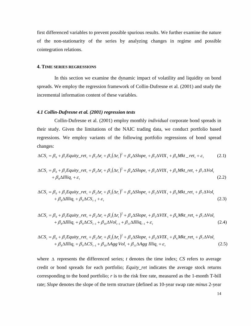
4.1 Collin-Dufresne et al. (2001) regression tests
Collin-Dufresne et al. (2001) employ monthly individual corporate bond spreads in
their study. Given the limitations of the NAIC trading data, we conduct portfolio based
regressions. We employ variants of the following portfolio regressions of bond spread
changes:
( )
( )
( )(2.3)
(2.2)
)1.2( _
198
7t6t5t42
32t10
8
7t6t5t42
32t10
t6t5t42
32t10
ttt
tttt
tt
tttt
tttt
CSIlliqVolMkt_retVIXSloperrEquity_retCS
IlliqVolMkt_retVIXSloperrEquity_retCS
retMktVIXSloperrEquity_retCS
εββββββββββ
εβββββββββ
εβββββββ
+∆+∆+∆++∆+∆+∆+∆++=∆
+∆+∆++∆+∆+∆+∆++=∆
++∆+∆+∆+∆++=∆
−
( )
( )(2.5)
(2.4)
1110198
7t6t5t42
32t10
111110198
7t6t5t42
32t10
ttttt
tttt
ttttt
tttt
IlliqAggVolAggCSIlliqVolMkt_retVIXSloperrEquity_retCS
IlliqVolCSIlliqVolMkt_retVIXSloperrEquity_retCS
εββββββββββββ
εββββββββββββ
+∆+∆+∆+∆+∆++∆+∆+∆+∆++=∆
+∆+∆+∆+∆+∆++∆+∆+∆+∆++=∆
−
−−−
where ∆ represents the differenced series; t denotes the time index; CS refers to average
credit or bond spreads for each portfolio; Equity_ret indicates the average stock returns
corresponding to the bond portfolio; r is to the risk free rate, measured as the 1-month T-bill
rate; Slope denotes the slope of the term structure (defined as 10-year swap rate minus 2-year

15
swap rate); Mkt_ret refers to the CRSP value weighted equity index return; Illiq represents
the average bond illiquidity of the underlying bond portfolio and refers to the bond illiquidity
factor obtained in Section 3.4; and Vol refers to the average equity volatility of the
corresponding bond portfolio. Regression (2.1) is similar to the equation 2 used in Collin-
Dufresne et al. (2001, page 2185).14 Regression (2.1) includes equity returns (as a proxy for
the firm’s health), risk-free rate and its squared term (for possible non-linear effects), term-
spread, aggregate stock market volatility and equity index returns. Regression (2.2) augments
Regression (2.1) with underlying idiosyncratic volatility and bond illiquidity. Regression
(2.3) includes the lagged credit spread variable to account for possible auto-correlations in
the dependent variable. Regression 2.4 (2.5) further augments Regression 3 with lagged
volatility and illiquidity (aggregate volatility and illiquidity15
[Insert Table 5 here]
) variables. We first implement
regressions for the pre-financial crisis period (1994-2007) in order to minimize the potential
impact of crisis-driven volatility on our results. We later study the effects of the crisis using
the complete sample in section 4.3.
Table 5 reports results for alternative regression models separately for different
monthly bond portfolios for the 1994-2007 period. Overall, we present eight regressions
(labeled A to H) for each portfolio. We also report heteroscedasticity-autocorrelation
consistent p-values based on the Newey and West (1987) procedure (with lag length set to
2). We observe that Regression A variables have the lowest explanatory power across
different portfolios, verifying the findings in Collin-Dufresne et al. (2001) that a large part of
the variation in credit spreads is not captured by such variables. Out of all the Regression A
variables, only four variables (i.e., underlying stock returns, nonlinear changes in risk-free
rate, aggregate stock market returns and VIX) have significant impact on bond spreads,
especially for the low-rated bond portfolio. We, however, notice that idiosyncratic volatility
has a significant contribution to the explanatory power of credit spreads for all bond
14 We are, however, missing the jump variable obtained as the slope of the implied volatility as we do not have the underlying option data. 15 Aggregate liquidity and volatility are based on the aggregate bond portfolio and corresponding equity portfolio, respectively.

16
portfolios, and the effect is strongly evident for low-rated, short- and long-term portfolios,
where the adjusted R2 values increase between 22%-30% based on Regressions A and B.
Bond illiquidity further increases the explanatory power of the regressions; the illiquidity
effect is strongly present for low-rated and short-term bond portfolios. Adding the illiquidity
factor increases the adjusted R2 values between 12%-22% based on Regressions A and C and
between 2%-11%, comparing Regressions B and D.
Further, comparing Regressions D and A in each panel we notice that volatility and
illiquidity together have the highest incremental effect for short-term bonds, followed by
low-rated bonds, where the adjusted R2 values go up by 40% and 24%, respectively. For
long-term bonds, volatility effect is highly significant and adds 30% to regression D.
Regressions E-G indicate that idiosyncratic volatility and illiquidity variables still remain
significant even after adding several control variables. The lagged bond spreads have
significant information content (particularly for high-rated and long-term bond portfolios),
indicating the persistence in time-series behavior of bond spreads. Lagged volatility and
illiquidity variables are not significant for any portfolio, implying that the impact of volatility
and liquidity on bond spreads is mostly contemporaneous.
Our results are robust to the inclusion of aggregate volatility and liquidity variables
for all the portfolios except the high-rated bonds, where the systematic volatility swamps the
individual volatility effect. Moreover, Regression E has the highest adjusted R2 values
overall and for low-rated, short- and long-term portfolios, indicating that once conditioned
for contemporaneous volatility and illiquidity, respective aggregate portfolio effects are
insignificant. Overall, we find that both idiosyncratic volatility and illiquidity effects
together have the highest impact for low-rated and short-term portfolios (Regression D),
while for others volatility remains the key driver.
We implement several robustness checks to test the validity of our results. First we
include portfolio stock liquidity based on Amihud’s measure (as defined in Table 2) as an
additional control variable and find the variable to be not significant. Second, we also
implement the regressions using weekly data and find qualitatively similar results. For
weekly trades, the illiquidity effect is even stronger for low-rated and long-term bonds.
Lagged volatility also matters in explaining the weekly bond spreads. Finally, we test if the
regression estimates on Table 5 are robust to the inclusion of industry production growth
17
proxies and interaction effects between (a) leverage and VIX and (b) bond illiquidity and
VIX. All results in Table 5 are robust to the inclusion of these control variables.16
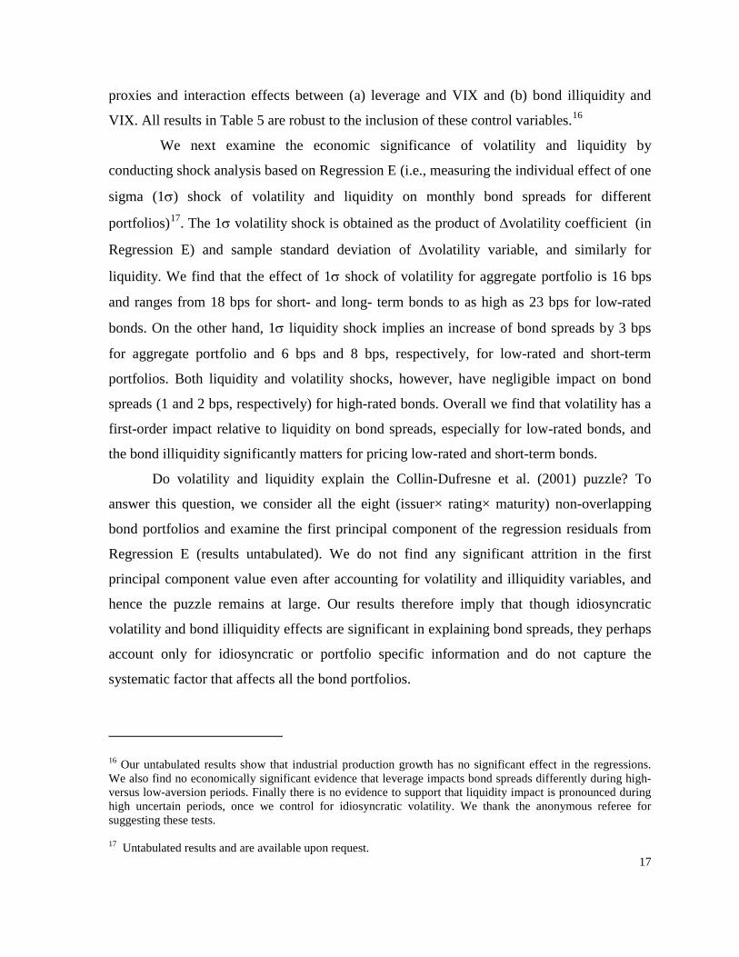
We next examine the economic significance of volatility and liquidity by
conducting shock analysis based on Regression E (i.e., measuring the individual effect of one
sigma (1σ) shock of volatility and liquidity on monthly bond spreads for different
portfolios)
17
Do volatility and liquidity explain the Collin-Dufresne et al. (2001) puzzle? To
answer this question, we consider all the eight (issuer× rating× maturity) non-overlapping
bond portfolios and examine the first principal component of the regression residuals from
Regression E (results untabulated). We do not find any significant attrition in the first
principal component value even after accounting for volatility and illiquidity variables, and
hence the puzzle remains at large. Our results therefore imply that though idiosyncratic
volatility and bond illiquidity effects are significant in explaining bond spreads, they perhaps
account only for idiosyncratic or portfolio specific information and do not capture the
systematic factor that affects all the bond portfolios.
. The 1σ volatility shock is obtained as the product of ∆volatility coefficient (in
Regression E) and sample standard deviation of ∆volatility variable, and similarly for
liquidity. We find that the effect of 1σ shock of volatility for aggregate portfolio is 16 bps
and ranges from 18 bps for short- and long- term bonds to as high as 23 bps for low-rated
bonds. On the other hand, 1σ liquidity shock implies an increase of bond spreads by 3 bps
for aggregate portfolio and 6 bps and 8 bps, respectively, for low-rated and short-term
portfolios. Both liquidity and volatility shocks, however, have negligible impact on bond
spreads (1 and 2 bps, respectively) for high-rated bonds. Overall we find that volatility has a
first-order impact relative to liquidity on bond spreads, especially for low-rated bonds, and
the bond illiquidity significantly matters for pricing low-rated and short-term bonds.
16 Our untabulated results show that industrial production growth has no significant effect in the regressions. We also find no economically significant evidence that leverage impacts bond spreads differently during high- versus low-aversion periods. Finally there is no evidence to support that liquidity impact is pronounced during high uncertain periods, once we control for idiosyncratic volatility. We thank the anonymous referee for suggesting these tests. 17 Untabulated results and are available upon request.

18
4.2 Expanded Collin-Dufresne et al. (2001) regression tests
We also investigate the following expanded version of the Regressions (2.1) and
(2.2) similar to Collin-Dufresne et al. (2001, page 2197):
( )( )
(3)
16151-t14
1-t131-t12111t10t93
8t7
t6t5t42
32t10
ttt
tt
ttt
IlliqVolMkt_retDef_spdVIXrHMLSMBrTED
Mkt_retVIXSloperrEquity_retCS
εββββββββββ
βββββββ
+∆+∆+++++++∆+
++∆+∆+∆+∆++=∆
−
The additional variables included are as follows: TED is the aggregate liquidity spread and is
measured as the 30-day LIBOR minus 3-month T-Bill rate; SMB and HML are Fama-French
equity market factors; Def_spd is the aggregate default spread and is measured as Moody’s
BAA yield minus 10- year swap rate. We also include the lagged interest rate ( 1tr − ), market
returns ( t-1Mkt_ret ) and VIX ( t-1VIX ) and the non-linear interest rate effects ( )2tr∆ and ( )3
tr∆
.18
[Insert Table 6 here]
As in the previous section, we first focus on the 1994-2007 sub-sample.
Results in Table 6 imply that idiosyncratic volatility continues to have a significant
explanatory power for credit spreads for all bond portfolios, adding 20% to 28% to the
adjusted R2 values for low-rated, short- and long-term bonds (comparing Regressions A and
B). The illiquidity effect is strongly present for low-rated and short-term bond portfolios and
increases the explanatory power by similar magnitudes as in Table 5. Regression D and E
results further show that both idiosyncratic volatility and illiquidity effects significantly
matter, once again, only for low-rated and short-term portfolios, while for others only
volatility matters. Moreover, comparing Table 5 and 6 results, we find that the highest
adjusted R2 values are still obtained using Regression E in Table 5.
4.3 Effects of the Financial crisis (2008-2010)
Here we reevaluate Table 5 and 6 regressions by extending the sample to include
the recent crisis period. Table 7 reports the incremental significance of idiosyncratic
18 We are, however, missing data on the firm-specific leverage used by Collin-Dufresne et al. (2001). We use TED spread in lieu of the aggregate liquidity proxies used by Collin-Dufresne et al. (2001).

19
volatility and bond illiquidity for different portfolios. While all the previous results hold, we
find that the coefficients of volatility and liquidity increase substantially, implying the
amplification of such effects on account of the crisis. Once the crisis period is included,
based on regression E from Panel A, we find that the effect of 1σ volatility shock on spreads
increases from 16 bps to 30 bps for aggregate portfolio, and from 6 to 54 (8 to 40) bps for
low-rated (short-term) bonds. Similarly 1σ liquidity shock engenders 19, 26 and 44 bps
impact on aggregate, low-rated, short-term portfolio spreads respectively, implying over
three-, four- or five-fold increases compared to pre-crisis period. Similar results follow from
panel B.19
[Insert Table 7 here]
4.4 Additional regressions with regime breaks
We next examine the robustness of the Collin-Dufresne et al. (2001) type
regressions in Section 4.1 by incorporating any possible structural breaks in the variables of
interest. Specifically, our objective is to test if changes in bond illiquidity and idiosyncratic
volatility across low or high regimes differentially impact credit spread changes.20
We first apply Hamilton’s (1989) two-state Markov regime-switching model to the
monthly portfolios of spreads, volatility and liquidity and identify the underlying regimes.
[Insert Figure 4 here]
Figure 4 plots the monthly time series of the key variables, along with the low- (i.e., the low-
mean-low-variance) and high- (i.e., the high-mean-high-variance) regimes.21
19 Results untabulated, and are available upon request.
For credit
spreads, the low-regime prevails during mid-2000 to mid-2003 (or end of 2004 depending
upon the portfolio) and also during the recent financial crisis period of 2008-10. For
idiosyncratic volatility we identify a clear regime break towards the end of 1998 (coinciding
20 Several previous papers explore the role of regimes in the dynamic behavior of corporate spreads, like Pedrosa and Roll (1998); Davies (2007, 2008); Avramov et al. (2007); Maalaoui et al. (2009); and Acharya et al. (2012). 21 In untabulated results, we find clear evidence of two regimes for all the analyzed variables. Differences in mean and variances for all regimes are different than zero, and results are consistent across weekly and monthly portfolios.

20
with the Russian debt crisis); we also observe a high-regime for volatility from 10/1998 to
06/2003 and again during the recent crisis. Switches in bond spreads seem to parallel low-
and high-regimes in equity volatility.22 Moreover, switches in idiosyncratic volatility seem to
lead bond-spread movements over time. For example, volatility first shifts to a high-regime
in late-98, followed by a similar switch in bond spreads later during mid-2000. Again
volatility reverts to a low regime in the middle of 2003, subsequently followed by bond
spreads; during late 2009, while volatility reverts to a low regime, bond spreads continue to
be in high regime. For the bond illiquidity measure, the regime switch to a permanent high
regime happens at the beginning of 2000, and no reversion to low-regime is evident until end
of the sample.23
Finally, we conduct regime-break regressions for various sub-portfolios, where
regimes for volatility and liquidity are pre-identified using Hamilton’s model. We employ
Regression (2.3) augmented with regime-specific dummies separately for volatility and
liquidity variables as shown below:
( )( ) ( ) ( )( ) (4) _
_ _ _
11110
987
t6t5t42
32t10
ttt
ttt
ttt
CSregIlliqHighIlliqregIlliqLowIlliqregVolHighVolregVolLowVol
Mkt_retVIXSloperrEquity_retCS
εβββββ
βββββββ
+∆+×∆+×∆+×∆+×∆
++∆+∆+∆+∆++=∆
−
where Low/High Vol_reg and Low/High Illiq_reg refer to dummy variables for low- or high-
volatility and illiquidity regimes, respectively. Regression 4 captures the differential effect of
low and high regimes on bond spreads.
[Insert Table 8 here]
Table 8 results imply that volatility overall has a pronounced impact mainly in high-regimes
for most of the portfolios. While volatility effects are significant in both volatility regimes
for low-rated and short rated portfolios, the high-regime coefficient seems to be higher.
22 In untabulated results, we also test for structural breaks using the CUSUM test (Brown et al., 1975) and find that the dates for the structural breaks obtained at the 1% significance level are almost identical to those from the Markov switching model. 23 We also model liquidity using a Markov- switching model with three regimes. The financial crisis periods are here identified as a third regime with higher mean and variance. However, the use of this more complicated model does not bring any additional insights to our reported regression results.
21
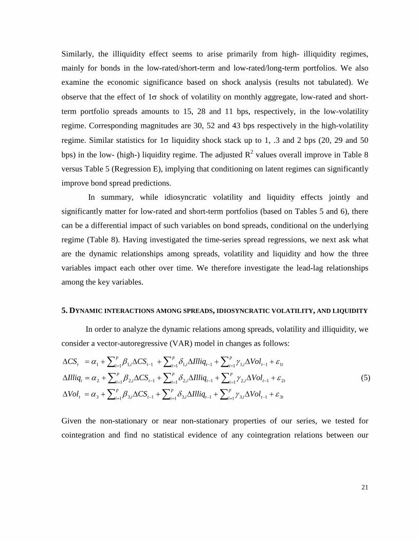
Similarly, the illiquidity effect seems to arise primarily from high- illiquidity regimes,
mainly for bonds in the low-rated/short-term and low-rated/long-term portfolios. We also
examine the economic significance based on shock analysis (results not tabulated). We
observe that the effect of 1σ shock of volatility on monthly aggregate, low-rated and short-
term portfolio spreads amounts to 15, 28 and 11 bps, respectively, in the low-volatility
regime. Corresponding magnitudes are 30, 52 and 43 bps respectively in the high-volatility
regime. Similar statistics for 1σ liquidity shock stack up to 1, .3 and 2 bps (20, 29 and 50
bps) in the low- (high-) liquidity regime. The adjusted R2 values overall improve in Table 8
versus Table 5 (Regression E), implying that conditioning on latent regimes can significantly
improve bond spread predictions.
In summary, while idiosyncratic volatility and liquidity effects jointly and
significantly matter for low-rated and short-term portfolios (based on Tables 5 and 6), there
can be a differential impact of such variables on bond spreads, conditional on the underlying
regime (Table 8). Having investigated the time-series spread regressions, we next ask what
are the dynamic relationships among spreads, volatility and liquidity and how the three
variables impact each other over time. We therefore investigate the lead-lag relationships
among the key variables.
5. DYNAMIC INTERACTIONS AMONG SPREADS, IDIOSYNCRATIC VOLATILITY, AND LIQUIDITY
In order to analyze the dynamic relations among spreads, volatility and illiquidity, we
consider a vector-autoregressive (VAR) model in changes as follows:
ttp
i itp
i itp
i it
ttp
i itp
i itp
i it
ttp
i itp
i itp
i it
VolIlliqCSVol
VolIlliqCSIlliq
VolIlliqCSCS
311 ,311 ,311 ,33
211 ,211 ,211 ,22
111 ,111 ,111 ,11
(5)
εγδβα
εγδβα
εγδβα
+∆+∆+∆+=∆
+∆+∆+∆+=∆
+∆+∆+∆+=∆
−=−=−=
−=−=−=
−=−=−=
∑∑∑∑∑∑∑∑∑
Given the non-stationary or near non-stationary properties of our series, we tested for
cointegration and find no statistical evidence of any cointegration relations between our

22
series.24
As a result, we do not include any error correction term in our estimation. We set
the number of lags used as three, based on the BIC and AIC selection criterion. All our VAR
specifications are stationary models, as we test whether all inverse roots of the characteristic
polynomial lie inside the unit circle.
5.1. Granger causality tests
We use the estimated parameters from the VAR model (5) to analyze how changes in
the lagged variables predict changes in their future values. Essentially, we want to explore
how bond spread changes can be predicted using past values of liquidity, of volatility or
both. Similarly, we study the predictability of volatility and liquidity based on past values of
the other variables in the VAR. We implement the Granger causality tests for these
hypotheses and summarize the results in Table 9.
[Insert Table 9 here]
We find strong evidence for volatility and illiquidity individually Granger-causing
bond spreads for all distress portfolios. Further, the joint test indicates that volatility and
illiquidity together Granger-cause spreads for all the three portfolios, implying that bond
prices slowly process information from other variables. The chi-squared test values and their
corresponding p-values also suggest that the effect of volatility is more persistent than that of
liquidity.
We observe that bond spreads Granger-cause volatility and illiquidity changes for all
the portfolios, confirming the feedback effects for distressed bonds. Finally, the Granger-
casualty results imply that illiquidity generally cannot be forecasted using past values of
spreads and volatility. It is, however, possible that past information in volatility and spreads
is quickly incorporated into market liquidity, and hence their effects are not observable at a
monthly frequency. Granger causality tests overall provide insights on differential lead-lag
interactions among the key variables. The next step is to analyze how unexpected shocks to
the variables influence their future values.
24 The number of lags is selected using the BIC and AIC selection criteria. All our VAR specifications are stationary models, as we test whether all inverse roots of the characteristic polynomial lie inside the unit circle.

23
5.2 Impulse response analysis
We analyze the short- and long-run impact of unexpected liquidity and volatility shocks
on credit spreads by employing the vector-autoregressive (VAR) model (5) described earlier.
We estimate the generalized impulse response functions and quantify the effects of current
unforecastable liquidity and volatility shocks on credit spreads. We follow Koop, Pesaran
and Potter (1996) and estimate the generalized impulse responses that are robust to variable
reorderings in the VAR. Monthly results for the accumulated generalized impulse response
functions for three different portfolios are presented in Table 10 and Figure 5. Since the
recent financial crisis may be interpreted as a large unanticipated volatility and liquidity
shock, impulse responses may behave very differently between crisis and non-crisis periods.
Accordingly, we first document a pre-crisis sample (1994-2007), where our results may be
interpreted as effects of "normal" shocks to volatility and liquidity; we next present impulse
response functions including the crisis period (1994-2010), and analyze the main differences.
[Insert Table 10 and Figure 5 here]
In Table 10, we report the accumulated impulse responses and the associated p-
values for sample periods with and without the recent financial crisis. Panel A, spanning the
1994-2007 period, shows that shocks to bond spreads are highly persistent over time. Current
period shock to spread has a strong effect (ranging between 39 and 66 bps) on the next
month’s spread, and a long-term impact of 23 to 40 bps after 10 months on future spreads.
All multi-period responses to a bond spread shock are significant at 10% level. The effect of
volatility shock on bond spreads ranges from 20 to 32 bps after one month and 7 to 14 bps
after ten months, and the shock effects are significant at both horizons. Relatively, the impact
of liquidity shock on spreads is weak; the short-term effect is 11 to 22 bps of higher spreads
after one month, while the cumulative long-term effect is small and not significantly
different from zero. Unlike the volatility shocks, the effect of liquidity shocks on bond
spreads is generally not significant after the first month.
Once we extend the sample to include the financial crisis period (i.e., 2008-10,
Panel B), magnitudes of the shock impact for all three variables (i.e., spreads, volatility and
liquidity) significantly increase across portfolios. Credit spread and volatility shocks are still
persistent and larger in magnitude compared to liquidity shocks as before. Liquidity shocks
now become more persistent and have a larger impact for low-rated and short-term

24
portfolios. However, as in the non- crisis subsample, the effect of liquidity shocks on bond
spreads is not consistently significant after the first month, and there is little evidence of a
long-term effect at the 5% significance level. 25
Similar results can be observed in Figure 5, where we plot the accumulated impulse
response functions and their corresponding 5% and 10% confidence bounds for sample
periods with (Panel A) and without (Panel B) the recent financial crisis.
Overall, our findings imply that the effects of volatility shocks are more persistent
and significant in magnitude; liquidity shocks in general are less persistent and seem to be
processed into bond prices under a month. Large liquidity and volatility shocks, as evidenced
during the recent financial crisis, increase the magnitude and persistency of the responses.
Volatility shocks, however, are still more persistent and have a significant long-run effect on
spreads compared to liquidity shocks, whose affects are mainly short-lived.
6. CHOLESKY VARIANCE DECOMPOSITION TESTS
Finally, we explore to what extent the volatility and liquidity variables can each
explain the error variance of bond spreads. The variance decomposition will enable us to
tease out the relative contribution of volatility and liquidity in explaining the residual bond
spreads. We follow a two step procedure: first, we use the Regression model (2.3) to estimate
bond spread residuals; second, we determine the contribution of volatility and liquidity
variables to the variance of the bond residuals, under two different orderings. We therefore
parse the total variance of residual bond spreads into information shares individually
explained by each of the regressors (i.e., volatility and liquidity) using the expressions under
Table 11. We obtain the variance shares for the pre-crisis and overall periods and separately
for the low- and high- bond spread, volatility and liquidity regimes.
[Insert Table 11 here]
25 In further untabulated results, we find that effects of contemporaneous shocks to the variables vary depending on the underlying bond ratings and maturities. The shock effects are stronger for low-rated versus high-rated bonds. While the volatility shocks have a similar effect on short- and long-term bonds, liquidity shocks matter only for the short-term bonds Impulse response analysis conducted using weekly data, which further confirms the monthly results.

25
The information shares for volatility and liquidity all increase in magnitude once we include
the financial crisis (Panel A). We observe that illiquidity can explain a significant residual
variance for short-term portfolios under the first ordering for the overall period (Panel A),
and that effect mainly is seen in the high-spread, high-volatility or high-illiquidity regime
(Panel B). Illiquidity is also important for the high-rated and high-rated long-term portfolio
bonds in the low-regimes (not tabulated). In all other cases, volatility has the dominant
explanatory power in both regimes and under different orderings.
7. Summary and Conclusions
In this paper we study the dynamic effects of idiosyncratic volatility and liquidity on
bond spreads over time. We analyze how such dynamic effects are impacted by underlying
portfolio characteristics and market regimes. Our study is unique in that we follow a
“ground-up” approach, where we employ an extensive sample of individual bond trades to
build aggregate bond portfolios and corresponding equity indices of interest.
We observe and document many critical differences between how volatility and
liquidity impact bond spread over time and across regimes. Our results imply that
idiosyncratic volatility and liquidity effects can significantly matter for the distress portfolios
(i.e., low-rated and short-term bonds), while for others volatility overwhelms liquidity.
Volatility, overall, has a first order-impact compared to bond illiquidity. Illiquidity shocks
are quickly processed into bonds prices, whereas volatility and credit (bond spread) shocks
are more persistent and have long-term effects. Both volatility and bond illiquidity shocks
are intensified during crisis regimes and tend to have larger and more persistent effect on
bond spreads.
Our results can be useful to wide interest groups. Practitioners may incorporate our
findings into improved pricing models based on differential impact of volatility and liquidity.
Investors can build better asset allocation and trading strategies.26
26 For example, long-horizon investors may find spreads from high-yield debt attractive, if such spreads are attributable to low liquidity rather than high default risk.
Debt issuers can
effectively manage their credit versus liquidity components of their funding costs by better
timing their debt issuance.

26
Determining the relative magnitudes and dynamic effects of credit versus liquidity
components is also vital for policy makers. If illiquidity is the main driver behind high
yields, measures to improve bond market liquidity are more appropriate. Liquidity shocks in
turbulent regimes can be virulent, as this study shows, and hence quick effort to contain the
funding risk mainly for low-rated and short-term issuers is imperative. This is partly because
both low-rated and short-term issuers will experience a sudden increase in yield spreads as
markets experience marked flights to quality and liquidity. Moreover deterioration in debt
market liquidity, particularly for financial firms, can engender severe funding difficulties and
further exacerbate their credit risk by intensifying their implicit rollover risk (He and Xiong,
2012). Early detection of liquidity-driven distress regimes can therefore help regulators
formulate better policy responses for financial bailouts and avoid costly liquidity-credit risk
spirals.
On the other hand, if bond spread changes are mainly impacted by default risks,
policy actions aimed at improving the solvency of the underlying banks and issuers become
critical. Unlike liquidity shocks, crisis induced volatility shocks are strong and persistent as
solvency of balance sheets, mainly consisting of low-rated, short-and long-term debt, is
adversely impacted. Therefore, identifying the differential characteristics of liquidity vs.
volatility shocks as documented in this study can enable better, more timely policy decisions.
Such a differential policy treatment was, for example, illustrated in the recent
financial crisis (for e.g., Sarkar, 2009). In particular, the Federal Reserve’s primary response
from 12/2007 to 03/2008 emphasized the provision of liquidity to solvent institutions as
illiquidity rather than credit risk seemed to be the main problem. In contrast, policy
initiatives starting in 09/2008 reflected the Federal Reserve's views of the increasing
importance of counterparty credit risk. Finally, our findings with respect to the persistence
and long-term effects of credit, liquidity and volatility shocks may also have direct policy
implications. For example, policy measures intended to improve credit and solvency
conditions and reduce volatility need to be long-term based, while those aimed at improving
liquidity need to focus on alleviating short-term funding squeezes.
27
Appendix A: Bond Sample Selection From the NAIC database, we first extract transaction information on U.S. corporate bond trades
between 1994 and 2010. The NAIC bond trades are then merged with various bond attributes from FISD. Based
on the 6-digit CUSIP numbers, the corporate bonds are further matched to the stock price data in the CRSP
database. Bond ratings on the transaction date of each bond trade are extracted from ratings tables in FISD. For
bond ratings, we use Standard & Poor’s (S&P) rating value if it exists; otherwise, we use Moody’s rating data.
On the transaction dates of bond trades, we compute yield-to-maturity and Macaulay duration based on reported
buy or sell prices and other related variables. We obtain yield spreads for each bond transaction using matching
maturity swap rates as benchmark (Houweling et al., 2005). Daily swap rates for 15 different maturities
(ranging between 1 and 30 years) are obtained from DATASTREAM. Each bond trade is matched to a
corresponding swap rate based on linear interpolation of the two closest neighboring maturity swap yields.
Since the tax treatment of swaps is similar to that of corporate bonds, the bond spreads with the swap
benchmark have little tax component in them (see Longstaff et al., 2005).
Several screening criteria are employed. From the NAIC database, we exclude bond trades
characterized by any of the following: (a) existing erroneous trade dates and incorrect third-party vendor
names; (b) underlying maturity less than one year on transaction date; (c) missing or extreme transaction prices
(transaction price is below $100 or above $10,000, where $1,000 is the par value); (d) variables needed to
compute yield-to-maturity missing or are erroneous; (e) inability to compute yield-to-maturity due to non-
convergence of pricing formula, or a computed yield greater than 100% or less than 1%; or (f) variables needed
to compute Macaulay duration missing or inability to compute Macaulay duration.
The following bond issues are further excluded: bonds with callable, redeemable, putable,
exchangeable, convertible, sinking fund, enhancement or asset-backed features; perpetual and variable rate
bonds; medium-term notes; Yankee, Canadian and foreign currency issues; Rule 144a issues; TIPS, Treasuries,
Munis, Treasury coupon- and principal-strips; and agency-type bonds. We also drop bond issues that are
unrated or have either missing or extreme bond ratings (below C grade or belonging to AAA or Aaa ratings27
27 Campbell and Taksler (2003) report pricing problems for high investment grade issues in the NAIC data.
).
Finally, we drop all bond trade observations that (a) do not have any matching stock in the CRSP database or
(b) have insufficient stock returns data in the six months prior to the bond transaction date (and hence equity
volatilities cannot be computed). All computed bond measures (yield-to-maturity, yield spread and duration)
are winsorized at the 1% level. The final matched dataset consists of issuance- and transaction-related
information on fixed-rate, U.S. dollar-denominated, domestic, straight corporate bond trades by all insurance
companies for publicly traded equity firms.

28
REFERENCES
Acharya, V., Amihud, Y., Bharath, S., 2012. Liquidity risk of corporate bond returns: A Conditional approach. Unpublished Manuscript. Stern School, NYU. Alexander, G., Edwards, A., Ferri, M., 2000a. What does NASDAQ’s high yield bond market reveal about bondholder-stockholder conflicts? Financial Management 29, 23-29. Alexander, G., Edwards, A., Ferri, M., 2000b. The determinants of trading volume of high yield corporate bonds. Journal of Financial Markets 3, 177-204. Alexander, C., Kaeck, A., 2008. Regime dependent determinants of credit default swap spreads. Journal of Banking and Finance 32, 1008–1021. Amihud, Y., 2002. Illiquidity and stock returns: Cross-section and time-series effects.
Journal of Financial Markets 5, 31-56. Avramov, D., Jostova, G., Philipov, A., 2007. Understanding corporate credit risk
changes, Financial Analysts Journal 63, 90-105. Bai, J., Ng., S., 2002. Determining the number of factors in approximate factor models.
Econometrica 70, 191-221. Bali, T., Cakici, N., Yan, X., Zhang, Z., 2005. Does idiosyncratic risk really matter? Journal
of Finance 60, 905-929. Bamber, L., Barron, O., Stober, T., 1999. Differential interpretations and trading volume.
Journal of Financial and Quantitative Analysis 34, 369-386. Bansal, N., Connolly, R.A., Stivers, C., 2009. Regime-switching in stock index and Treasury
futures returns and measures of stock market stress. Working paper, University of North Carolina.
Bao, J., Pan, J., 2008. Excess volatility of corporate bonds. Working paper, Massachusetts Institute of Technology.
Bao, J., Pan, J., Wang J., 2011. The illiquidity of corporate bonds. The Journal of Finance 66, 911–946.
Beber, A., Brandt, M., Kavajecz, K., 2009. Flight-to-quality or flight-to-liquidity? Evidence from the euro-area bond market? Review of Financial Studies 22, 925-957.
Bernanke, B., Boivin, J., Eliasz, P., 2005. Measuring monetary policy: A factor augmented vector autoregressive (FAVAR) approach. Quarterly Journal of Economics 120, 387-422.
Bessembinder, H., Maxwell, W., Venkataraman, K., 2006. Market transparency, liquidity externalities, and institutional trading costs in corporate bonds. Journal of Financial Economics 82, 251-288.
Boehme, R., Danielsen, B., Sorescu, S., 2006. Short-sale constraints, differences of opinion, and overvaluation. Journal of Financial and Quantitative Analysis 41, 455-487.
Brunnermeier, M., 2009. Deciphering the liquidity and credit crunch 2007-08. Journal of Economic Perspectives 23, 77-100.
Brunnermeier, M., Pedersen, L., 2009. Market liquidity and funding liquidity. Review of Financial Studies 22, 2201-2238.
Buraschia, A., Menini, D., 2002. Liquidity risk and specialness. Journal of Financial Economics 64, 243-284.
Campbell, J., Lettau, M., Malkiel, B., Xu, Y., 2001. Have individual stocks become more volatile? An empirical explanation of idiosyncratic risk. Journal of Finance 56, 1-43.
Campbell, J., Taksler, G., 2003. Equity volatility and corporate bond yields. Journal of Finance 58, 2321-2349.
29
Chen, L., Lesmond, D., Wei, J., 2007. Corporate yield spreads and bond liquidity. Journal of Finance 62, 119-149.
Chen, T., Liao, H., Tsai, P., 2011, Internal liquidity risk in corporate bond yield spreads, Journal of Banking and Finance 35,4, 978-987.
Chordia, T., Sarkar, A., Subrahmanyam, A., 2005. An empirical analysis of stock and bond market liquidity. Review of Financial Studies 18, 85-129.
Collin-Dufresne, P., Goldstein, R.S., Martin, J.S., 2001. The determinants of credit spread changes. Journal of Finance 56, 2177-2207.
Connolly, R., Stivers, C., Sun, L., 2005. Stock market uncertainty and the stock-bond return relation. Journal of Financial and Quantitative Analysis 40, 161-194.
Connolly, R., Stivers, C., Sun, L., 2007. Commonality in the time-variation of stock-stock and stock-bond return comovements, Journal of Financial Markets 10, 192-218.
Covitz, D., Downing, C., 2007. Liquidity or credit risk? The determinants of very short-term corporate yield spreads. Journal of Finance 62, 2303-2328.
Cremers, M., Driessen, J., Maenhout, P., 2008a. Explaining the level of credit spreads: Option-implied jump risk premia in a firm value model. Review of Financial Studies 21, 2209-2242. Cremers, M., Driessen, J., Maenhout, P., Weinbaum, D., 2008b. Individual stock-option prices and credit spreads. Journal of Banking and Finance 32, 2706-2715. Davies, A., 2008. Credit spread determinants: An 85 year perspective, Journal of Financial Markets 11, 180–197. Das, S., Hanouna, P., 2009, Implied recovery, Journal of Economic Dynamics and Control, 33, 11, 1837-1857. Das, S., Sundaram, R., 2007. An integrated model for hybrid securities. Management Science 53, 1439–1451. Downing, C., Underwood, S., Xing, Y., 2009. The relative informational efficiency of stocks and bonds: An intraday analysis. Journal of Financial and Quantitative Analysis 44, 1081-1102. Downing, C., Underwood, S., Xing, Y. 2005., Is liquidity risk priced in the corporate bond market?, Working paper, Rice University. Driessen, J., 2005. Is default event risk priced in corporate bonds? Review of Financial
Studies 18, 165-195. Duarte, J., Longstaff, F., Yu, F., 2005. Risk and return in fixed income arbitrage: Nickels in
front of a steamroller? Review of Financial Studies 20, 769-811. Edwards, A., Harris, L., Piwowar, M., 2007. Corporate bond market transparency and
transactions costs. Journal of Finance 62, 1421-1451. Ericsson, J., Renault, E., 2006. Liquidity and credit risk. Journal of Finance 61, 2219-2256. Ericsson, J., Jacobs, K., Oviedo, R., 2009. The determinants of credit default swap premia.
Journal of Financial and Quantitative Analysis 44, 109-132. Fama, E., French, K., 1993. Common risk factors in the returns of stocks and bonds. Journal
of Financial Economics 33, 3-56. Fleming, J., Kirby, C., Ostdiek, B., 1998. Information and volatility linkages in the stock,
bond, and money markets. Journal of Financial Economics 49:1, 111–137. Gady, J., Theocharides, G., Zheng, S., 2007. Liquidity risk in the corporate bond market.
Working paper, University of Manitoba.
30
Gebhardt, W., Hvidkjaer, S., Swaminathan, B., 2005a. The cross-section of expected corporate bond returns: Betas or characteristics? Journal of Financial Economics 75, 85-114.
Gebhardt, W., Hvidkjaer, S., Swaminathan, B., 2005b. Stock and bond market interaction: Does momentum spill over? Journal of Financial Economics 75, 651-690.
Gilchrist, S., Yankov, V., Zakrajsek, E., 2009. Credit market shocks and economic Fluctuations: Evidence from corporate bond and stock markets. Journal of Monetary Economics 56, 471-493
Goyenko, R., Ukhov, A., 2009. Stock and bond market liquidity: A long-run empirical analysis. Journal of Financial and Quantitative Analysis 44, 189-212.
Güntay, L., Hackbarth, D., 2010. Corporate bond credit spreads and forecast dispersion Journal of Banking and Finance 34, 10, 2328-2345.
Hamilton, J., 1989, A new approach to the economic analysis of nonstationary time series and the business cycle. Econometrica 57, 357-384.
Han, S., Zhu, H., 2008. Effects of liquidity on the non-default component of corporate yield spreads: Evidence from intraday transactions data. Working paper, Federal Reserve Board.
Harris, M., Raviv, A., 1993. Differences of opinion make a horse race. Review of Financial Studies 6, 473-506.
He, Z. and W. Xiong, 2012. Rollover risk and credit risk, Journal of Finance, Vol. XVII, 2, 391-427.
Henderson, B., Narasimhan, J., Weisbach, M., 2006. World markets for raising new capital. Journal of Financial Economics 82, 63-101.
Hong, G., Warga, A., 2000. An empirical study of bond market transactions. Financial Analysts Journal 56, 32-46.
Hotchkiss, E., Ronnen, T., 2002. The informational efficiency of the corporate bond market: An intra-day analysis. Review of Financial Studies 15, 1325-1354.
Houweling, P., Mentink, A., Vorst, T., 2005. Comparing possible proxies of bond liquidity. Journal of Banking and Finance 29, 1331-1358.
Huang, J., Huang, M., 2003. How much of the corporate treasury yield spread is due to credit risk? Unpublished Manuscript. Penn State University.
Jankowitsch, R., Nashikkar, A., Subrahmanyam, M., 2011. Price dispersion in OTC markets: A new measure of liquidity. Journal of Banking and Finance 35, 343-357.
Kalimipalli, M., Warga, A., 2002. Bid/ask spreads, volume and volatility in the corporate bond market. Journal of Fixed Income 11, 31-42.
Kalimipalli, M., Nayak, S., 2012. Liquidity vs. volatility? Evidence from the US corporate bond market. Journal of Financial Intermediation, 21(2), 217-242.
Kandel, E., Pearson, N., 1995. Differential interpretation of public information and trade in speculative markets. Journal of Political Economy 103, 831-872.
Koop, G., M. H. Pesaran, and S. M. Potter, Simon, 1996. Impulse response analysis in Nonlinear multivariate models. Journal of Econometrics, 74(1),119-147 .
Krishnan, C. N. V., Ritchken, P. H., Thomson, J. B., 2010. Predicting credit spreads. Journal of Financial Intermediation 19, 529-563.
Kwan, S., 1996. Firm specific information and the correlation between individual stocks and bonds. Journal of Financial Economics 40, 63-80.
Liu, J., Longstaff, F. A., and Mandell, R.E., 2006. The market price of risk in interest rate

31
swaps: The roles of default and liquidity risk. Journal of Business 79, 5, 2337-2359. Lo, A., Mamaysky, H., Wang, J., 2004. Asset prices and trading volume under fixed
transactions costs. Journal of Political Economy 112, 1054-1090. Longstaff, F., Mithal, S., Neis, E., 2005. Corporate yield spreads: Default or liquidity?
Evidence from the CDS market. Journal of Finance 60, 2213-2253. Maalaoui, O., Dionne, G., François, P., 2009. Credit spread changes within switching
regimes, Working paper, HEC Montréal. Mahanti, S., Nashikkar, A., Subrahmanyam, M., Chacko, G., Mallik, G., 2008. Latent
liquidity: A new measure of liquidity, with an application to corporate bonds. Journal of Financial Economics 88, 272-298.
Maxwell, W., Stephens, C., 2003. The wealth effects of repurchases on bondholders. Journal of Finance 63, 895-919.
McInish, T., Wood, R., 1992. An analysis of intraday patterns in bid/ask spreads for NYSE stocks. Journal of Finance 57, 753-764.
Merton, R., 1974. On the pricing of corporate debt: The risk structure of interest rates. Journal of Finance 29, 449-470.
Newey, W.K., West, K.D., 1987. A simple, positive semi-definite, heteroskedasticity and autocorrelation consistent covariance matrix. Econometrica 55, 3,703–708.
O’Hara, M., 2003. Liquidity and price discovery. Journal of Finance 63, 1335-1354. Pedrosa, M., Roll, R., 1998. Systematic risk in corporate bond credit spreads. Journal of
Fixed Income 8, 7-26. Roll, R., 1984. A simple implicit measure of the effective bid-ask spread in an efficient
market. Journal of Finance 39, 1127-1139. Sarkar, A., 2009. Liquidity risk, credit risk, and the Federal Reserve’s responses to the crisis,
FRBNY Staff Reports. Schultz, P., 2001. Corporate bond trading costs: A peek behind the curtain. Journal of
Finance 56, 677-698. Schwartz, K, 2010. Mind the gap: Disentangling credit and liquidity in risk spreads. Working
paper, University of Pennsylvania. Spiegel, M., Wang, X., 2005. Cross-sectional variation in stock returns: Liquidity and
idiosyncratic risk. Working paper, Yale University. Stock, J., Watson, M., 2002. Macroeconomic forecasting using diffusion indexes. Journal of
Business Economics and Statistics 20, 147-162. Tang, D., Yan, H., 2010. Market conditions, default risk and credit spreads. Journal of
Banking & Finance 34, 4, 743-753. Underwood, S., 2009, The cross-market information content of stock and bond order flow.
Journal of Financial Markets 12, 2, 268-289. Van Landschoot, A., 2008. Determinants of yield spread dynamics: Euro versus US dollar
corporate bonds. Journal of Banking and Finance, 32,12, 2597–2605. Yu, F., 2006. How profitable is capital structure arbitrage? Financial Analysts Journal 62,
47-62. Zhang, B.Y., Zhou, H., Zhu, H., 2009. Explaining credit default swap spreads with the equity
volatility and jump risks of individual firms. Review of Financial Studies 22, 5099-5131.

1
Table 1 Summary statistics of bonds underlying bond portfolios (1994-2010) Panel A reports the number of observations of bond trades and average % yield spreads (first and second rows, respectively) for different sub-samples of bonds based on industry, rating and maturity categories for different time-periods. FIN, IND and UTL refer to Financial, Industrial, and Utility firms. Rating ≤BB indicates bonds with BB or lower ratings. Panel B further reports the same metrics for different rating-industry subsamples for each maturity and time period. Missing observations in Panel B refer to zero bond trades for a given sub-category. Panel A: Number of bond trades and bond spreads by industry, rating and maturity categories, for different sub-sample periods
FIN IND UTL AA A BBB ≤BB TotalBy MaturityLong-Term 5,451 23,920 1,832 3,113 14,914 10,440 2,736 31,203> 15 years 1.19 1.53 1.51 0.68 0.89 1.64 4.83 1.47
Medium-Term 24,035 31,119 5,395 7,341 31,177 16,727 5,304 60,5497-15 years 0.68 1.06 0.76 0.29 0.53 0.97 3.51 0.88
Short-Term 46,934 54,367 11,217 12,536 57,866 31,527 10,589 112,5181-7 years 0.87 1.49 1.47 0.34 0.55 1.26 5.91 1.23
By Time Period1994-1999 36,827 54,143 10,774 12,696 51,416 31,290 6,342 101,744
0.47 0.62 0.46 0.20 0.37 0.70 1.99 0.55
2000-2004 30,315 43,227 6,413 7,813 41,384 22,064 8,694 79,9550.85 2.05 2.54 0.43 0.73 1.84 6.49 1.63
2005-2007 5,817 7,512 840 1,538 7,178 3,361 2,092 14,1690.41 1.28 1.20 0.32 0.36 0.91 3.30 0.92
2008-2010 3,461 4,524 417 943 3,979 1,979 1,501 8,4025.33 4.11 2.84 2.20 2.54 3.85 12.28 4.55
Total 76,420 109,406 18,444 22,990 103,957 58,694 18,629 204,2700.84 1.38 1.27 0.37 0.59 1.24 5.07 1.16
By Industry By Rating

2
Table 1. Panel B: Number of bond trades and bond spreads by rating, industry, and maturity sub-groups for different sub-sample periods
FIN IND UTL FIN IND UTL FIN IND UTL FIN IND UTL Total
Long-Term 611 832 159 1,395 4,795 164 372 3,360 456 -- 665 53 12,862> 15 years 0.69 0.49 0.53 0.80 0.67 0.64 1.20 1.10 1.01 2.22 1.06 0.89
Medium-Term 2,072 2,641 779 10,284 7,814 1,344 2,373 7,513 1,481 179 1,859 521 38,8607-15 years 0.32 0.08 0.11 0.41 0.29 0.23 0.63 0.67 0.53 2.73 1.92 1.50 0.51
Short-Term 1,954 2,763 885 13,953 9,614 2,053 3,455 9,907 2,373 179 2,380 506 50,0221-7 years 0.25 0.04 0.12 0.35 0.25 0.21 0.61 0.67 0.47 5.72 1.95 1.16 0.49
Total 4,637 6,236 1,823 25,632 22,223 3,561 6,200 20,780 4,310 358 4,904 1,080 101,7440.34 0.12 0.15 0.40 0.36 0.24 0.65 0.74 0.55 4.22 1.97 1.32 0.55
Long-Term 389 671 46 1,529 4,783 155 285 4,134 429 14 907 150 13,492> 15 years 0.82 0.45 0.66 0.89 0.95 0.65 2.18 1.91 1.83 12.47 5.77 4.01 1.63
Medium-Term 778 556 39 5,270 3,177 511 601 3,054 376 70 1,540 205 16,1777-15 years 0.63 0.19 0.33 0.74 0.70 0.56 1.43 1.51 1.62 3.33 4.68 5.09 1.33
Short-Term 3,153 1,984 197 16,207 8,061 1,691 1,598 9,855 1,732 421 4,505 882 50,2861-7 years 0.51 0.17 0.87 0.68 0.69 0.63 1.60 1.87 2.42 5.87 7.12 8.37 1.73
Total 4,320 3,211 282 23,006 16,021 2,357 2,484 17,043 2,537 505 6,952 1,237 79,9550.56 0.23 0.76 0.71 0.77 0.62 1.63 1.82 2.20 5.70 6.41 7.29 1.63
Long-Term 58 137 4 302 892 28 51 779 34 22 563 54 2,924> 15 years 0.83 0.50 0.56 0.69 0.68 0.66 1.94 1.62 1.48 2.87 4.01 2.18 1.64
Medium-Term 252 36 -- 1,265 421 53 99 631 32 52 501 1 3,3437-15 years 0.67 0.19 0.45 0.49 0.44 0.62 1.11 0.46 1.86 3.08 1.27 1.01
Short-Term 734 317 -- 2,630 1,315 272 328 1,126 281 24 794 81 7,9021-7 years 0.25 0.01 0.26 0.18 0.14 0.49 0.53 0.34 1.66 2.70 7.96 0.61
Total 1,044 490 4 4,197 2,628 353 478 2,536 347 98 1,858 136 14,1690.39 0.16 0.56 0.35 0.40 0.22 0.67 1.01 0.47 2.04 3.20 5.61 0.92
Long-Term 75 129 2 234 593 44 74 441 25 40 239 29 1,925> 15 years 2.68 1.85 2.30 3.16 2.11 1.92 4.92 3.09 3.81 8.03 11.49 5.77 3.94
Medium-Term 147 41 -- 442 577 19 103 434 30 48 324 4 2,1697-15 years 2.36 1.70 3.57 1.72 2.06 5.94 2.92 2.97 11.61 9.48 4.53 3.98
Short-Term 394 155 -- 1,361 535 174 256 567 49 287 489 41 4,3081-7 years 2.71 0.92 3.25 1.32 1.59 8.04 2.87 2.84 21.54 10.44 6.54 5.11
Total 616 325 2 2,037 1,705 237 433 1,442 104 375 1,052 74 8,4022.62 1.39 2.30 3.31 1.73 1.69 7.01 2.95 3.11 18.83 10.38 6.13 4.55
AA
Sub-Sample: 2005-2007
Sub-Sample: 2008-2010
A BBB ≤BB
Sub-Sample: 1994-1999
Sub-Sample: 2000-2004

3
Table 2 Variable definitions The table defines different variables and portfolios used in the paper.
Portfolios: Overall, we consider 8 equally weighted portfolios: 2 industries (Industrials and non-Industrials) × 2 ratings (high and low) × 2 maturity (short- and long- term) categories. Low (high-) -ratings refer to bonds rated BBB and below (AA or A). Short- (long-) term bonds refer to maturities ≤ 7 years ( > 7) years. For each portfolio, we obtain equally weighted indices of bond spreads, equity volatility and bond/equity liquidity. Bond spread (Data Sources: DATASTREAM, NAIC) Yield spread is obtained as the bond yield minus equal maturity swap yield, linearly interpolated from daily swap rates. Equity Volatility measures (Data Sources: CRSP, Wharton Research Data Services or WRDS) 1) Id. Volatility (3-factor, daily or monthly): Idiosyncratic volatility computed as the variance of residuals
from the application of the Fama-French 3-factor model on 125 days (or 6 months) of daily (or monthly) stock returns prior to the transaction date.
2) Id. Volatility (4-factor, daily or monthly): Idiosyncratic volatility computed as the variance of residuals from the application of the Fama-French 4-factor model on 125 days (or 6 months) of daily (or monthly) stock returns prior to the transaction date.
Bond Liquidity measures (Data Sources: FISD, NAIC) Trade variables 1) Trade size (in 000’s of dollars): based on NAIC variable “actual_cost” if it is a buy trade, and NAIC
variable “consideration” if it is a sell trade. Higher trade size is associated with lower transaction costs and hence higher liquidity (Edwards et al., 2006).
2) Annual trading frequency: number of transactions in one year prior to the transaction date. The higher the trading frequency, the more actively the bond is traded, and hence liquidity is higher (Edwards et al., 2006).
Price Impact variables 3) Bond liquidity index 1: bond price impact variable calculated based on the transaction prices of all trades in
one year prior to the transaction date as: ( ) volumetotal10 prices8 σ× , where σprices is the standard deviation
of transaction prices of all trades and total volume is the dollar volume of all trades in the one-year window prior to the transaction date. Higher price impact values imply lower liquidity (Gady et al., 2007).
4) Bond liquidity index 2: bond price impact variable calculated based on the transaction prices of all trades in the one-year window prior to the transaction date as:
8 maximum price minimum price10 total volumeaverage price
−×
, where the maximum, minimum and average
prices, respectively, denote the highest, lowest and mean prices based on all the observed trades over the last year, and total volume is defined as in variable 3 above. Higher price impact values imply lower liquidity (Edwards et al., 2006).
We next employ a principal component procedure (Bai and Ng, 2002) to combine the four bond liquidity series for each portfolio. The first principal component obtained from the procedure is referred to as the bond illiquidity in the subsequent exhibits. Equity Liquidity (Data Sources: CRSP) Inverse of Amihud (2002) equity impact measure computed over a 125-day window as inverse of
( )125
8
110 returns $ trading volume 125t k t k
k− −
=
×∑ (excluding days of zero trading volume). It measures the
inverse of the cumulative price impact of order flow. Lower price impact values imply higher illiquidity. Aggregate market factors (Data Sources: 1,2,3,6:DATASTREAM; 4:NAIC; 5,7,8:WRDS) 1). Term-structure factor (Slope): 10-year swap rate minus 2-year swap rate; 2). Default factor (Def_spd): Moody’s BAA yield minus 10-year swap rate; 3). Aggregate liquidity factor (TED): 30-day LIBOR minus 3- month T-Bill rate; 4). Aggregate bond illiquidity factor (Agg Illiq): equally-weighted average of aggregate bond portfolio liquidity index 1 values each month; 5). Risk-free rate: 1-month T-bill rate; 6). Equity market volatility factor: VIX index; 7). Aggregate idiosyncratic volatility factor (Agg Vol): equally-weighted average of idiosyncratic volatilities of all equities underlying the overall bond portfolio each month; and 8). Equity market factors: Small minus big (SMB) size, high minus low book-to-market (HML) value and momentum factors.

4
Table 3 Summary statistics of bond portfolios Panel A presents the summary statistics (i.e., mean, median, maximum, minimum, standard deviation, skewness and kurtosis) for portfolio credit spreads, idiosyncratic equity volatility and bond illiquidity, as defined in Table 2. We consider the overall value-weighted Industrial portfolio, and different sub-sample portfolios of Industrial bonds based on ratings and maturity, both for the pre-crisis period (1994-2007) and crisis-period (2008-10). Low-rated (high-rated) portfolio consists of bonds rated BBB and below (above BBB, i.e., AA or A). Short- (long-) term portfolios have bonds with maturities 7 years or below (greater than 7 years). Panel B reports correlations among the key variables, along with respective p-values, for different portfolios. Finally, Panel C reports correlations (and respective p-values) for first differenced variables. ***, ** and *, respectively, refer to significance at 1%, 5% and 10% levels. Panel A: Summary statistics
Mean Med. Max. Min.Std. dev. Skew. Kurt. Mean Med. Max. Min.
Std. dev. Skew. Kurt.
Aggregate portfolio 1.226 1.061 3.142 0.302 0.741 0.804 2.680 4.160 3.311 10.624 1.705 2.329 1.321 3.616High-rated portfolio 0.433 0.358 1.201 0.071 0.231 1.127 3.586 1.661 1.376 3.362 0.824 0.699 0.847 2.428Low-rated portfolio 1.893 1.597 5.420 0.488 1.162 0.938 3.022 6.327 5.028 19.404 2.558 4.076 1.566 4.584Short-term portfolio 1.182 0.829 3.773 0.074 0.937 1.105 3.087 4.129 3.687 9.889 1.137 2.529 0.826 2.583Long-term portfolio 1.231 1.193 3.207 0.346 0.626 0.556 2.676 4.184 3.053 11.958 1.881 2.416 1.625 4.958Idiosyncratic VolatilityAggregate portfolio 0.098 0.069 0.263 0.032 0.061 1.098 2.967 0.135 0.095 0.472 0.033 0.113 1.603 4.599High-rated portfolio 0.071 0.056 0.215 0.023 0.046 1.443 4.378 0.069 0.051 0.162 0.024 0.041 0.921 2.536Low-rated portfolio 0.122 0.083 0.353 0.039 0.077 1.069 2.904 0.206 0.131 0.780 0.045 0.190 1.567 4.522Short-term portfolio 0.102 0.069 0.291 0.032 0.066 1.101 3.077 0.149 0.098 0.539 0.026 0.129 1.363 4.086Long-term portfolio 0.093 0.066 0.246 0.032 0.055 1.124 3.014 0.123 0.089 0.470 0.035 0.103 1.890 5.974Bond Illiquidity ( × 100)Aggregate portfolio -2.103 -2.194 13.002 -11.114 4.299 0.437 3.11 9.812 7.726 30.239 -6.665 8.792 0.503 2.715High-rated portfolio -1.317 -2.845 28.757 -10.652 6.134 1.827 7.422 6.148 5.471 29.478 -4.767 7.679 1.211 4.788Low-rated portfolio -1.894 -1.881 18.965 -15.752 4.747 0.342 4.19 8.837 9.284 32.505 -7.723 8.981 0.478 3.523Short-term portfolio -0.908 -0.809 14.895 -12.943 5.009 0.227 3.191 4.24 1.341 53.312 -7.608 11.98 2.329 9.157Long-term portfolio -1.891 -2.248 20.379 -13.256 4.585 0.793 5.272 8.827 9.451 34.227 -16.494 9.385 0.016 3.805
1994-2007 2008-2010
Spreads (%)

5
Table 3 Contd. Summary statistics of bond portfolios Panel B: Correlations among levels
Panel C: Correlations among changes
Spread-Idio. Vol.
p-val
Spread-Illiquidity
p-val
Illiquidity-Idio. Vol.
p-val
Spread-Idio. Vol.
p-val
Spread-Illiquidity
p-val
Illiquidity-Idio. Vol.
p-val
Aggregate portfolio 0.523 *** 0.256 *** -0.219 *** 0.932 *** 0.462 *** 0.413 ***High-rated portfolio 0.300 *** -0.274 *** -0.313 *** 0.791 *** 0.013 -0.204Low-rated portfolio 0.621 *** 0.473 *** 0.014 0.935 *** 0.604 *** 0.588 ***Short-term portfolio 0.643 *** 0.294 *** -0.089 0.848 *** 0.549 *** 0.255Long-term portfolio 0.290 *** 0.424 *** -0.240 *** 0.927 *** 0.493 *** 0.514 ***
1994-2007 2008-10
∆Spread-∆Idio. Vol.
p-val
∆Spread-∆Illiquidity
p-val
∆Illiquidity-∆Idio. Vol.
p-val
∆Spread-∆Idio. Vol.
p-val
∆Spread-∆Illiquidity
p-val
∆Illiquidity-∆Idio. Vol.
p-val
Aggregate portfolio 0.567 *** 0.390 *** 0.371 *** 0.593 *** 0.506 *** 0.264 *High-rated portfolio 0.189 ** 0.146 * 0.073 0.236 0.191 -0.023Low-rated portfolio 0.489 *** 0.282 *** 0.290 *** 0.630 *** 0.524 *** 0.381 **Short-term portfolio 0.567 *** 0.461 *** 0.310 *** 0.557 *** 0.680 *** 0.213Long-term portfolio 0.556 *** 0.154 ** 0.166 ** 0.713 *** 0.306 * 0.419 ***
1994-2007 2008-10

6
Table 4 Augmented Dickey Fuller (ADF) tests for unit roots (1994-2010) This table reports p-values for the null hypothesis that the monthly data series follows a unit root process using the ADF test. We consider equally weighted indices of credit spreads, bond illiquidity and idiosyncratic volatility for different industrial bond portfolios (as defined in Table 2) for both the pre-crisis period (1994-2007) and the full sample period (2008-10). Lags are selected using the BIC. Results are reported using deterministic trends and without trends. Low-rated (high-rated) portfolio consists of bonds rated BBB and below (above BBB, i.e., AA or A). Short- (long-) term portfolios have bonds with maturities 7 years or below (greater than 7 years).
No trend Trend lags No trend Trend lags No trend Trend Aggregate portfolio 0.39 0.57 0 0.32 0.63 1 0.79 0.01High-rated portfolio 0.23 0.40 0 0.63 0.84 0 0.17 0.00Low-rated portfolio 0.36 0.52 1 0.39 0.71 1 0.81 0.04Short-term portfolio 0.33 0.62 3 0.30 0.60 1 0.37 0.00Long-term portfolio 0.28 0.01 1 0.48 0.77 0 0.03 0.00
No trend Trend lags No trend Trend lags No trend Trend Aggregate portfolio 0.23 0.26 7 0.05 0.16 1 0.02 0.00High-rated portfolio 0.07 0.05 2 0.19 0.29 4 0.90 0.00Low-rated portfolio 0.04 0.03 0 0.03 0.11 4 0.26 0.00Short-term portfolio 0.08 0.10 5 0.03 0.13 5 0.03 0.00Long-term portfolio 0.07 0.03 4 0.01 0.03 0 0.29 0.00
2
1994-2007Credit Spreads Idiosyncratic Volatility Bond Illiquidity
lags2222
0011
1994- 2010Credit Spreads Idiosyncratic Volatility Bond Illiquidity
lags1

7
Table 5 Monthly Collin-Dufresne et al. (2001) time-series regression tests for volatility and liquidity (1994-2007) In this table, we implement Collin-Dufresne et al. (2001; page 2185, eq 2) type regressions and test for the incremental significance of idiosyncratic volatility and bond illiquidity for different monthly portfolios from 1994 to 2007. We employ Regressions (2.1) to (2.5) in the paper, and regress portfolio bond spreads (CS) on several time-series variables: Equity _ret (the equally weighted stock returns corresponding to the bond portfolio); r (the risk free rate); Slope (the slope of the term structure); Mkt_ret (the CRSP value weighted equity index return); Vol (the equally weighted equity volatility corresponding to the underlying bond portfolio); Illiq (the equally weighted bond illiquidity of the underlying bond portfolio and refers to the bond illiquidity factor); Agg Vol (the equally weighted equity volatility underlying the overall bond portfolio); and Agg Illiq (the equally weighted bond illiquidity of the overall bond portfolio). For each regression, we report heteroscedasticity-autocorrelation consistent p-values based on the Newey-West procedures (1987) (in italics), adjusted R2 values (adj R2) and respective number of observations (NOBS). Significant variables (at 10% significance level or below) in each regression are highlighted in bold. Low-rated (high-rated) portfolio consists of bonds rated BBB and below (above BBB, i.e., AA or A). Short- (long-) term portfolio has bonds with maturities 7 years or below (greater than 7 years).
Constant Equity_rett Δrt (Δrt)2 Δ Slopet ΔVIXt Mkt_rett ΔVolt ΔIlliqt ΔCSt-1 ΔVolt-1 ΔIlliqt-1
ΔAgg Volt
ΔAgg Illiqt Adj R2 NOBS
0.017 -0.010 -0.032 -7.073 0.057 0.016 0.019 0.018 1670.366 0.136 0.956 0.269 0.781 0.011 0.012
0.032 -0.010 -0.241 -11.517 0.058 0.008 0.008 10.252 0.324 167
0.149 0.108 0.615 0.018 0.684 0.103 0.282 0.000
0.019 -0.011 -0.536 -8.661 -0.019 0.012 0.017 1.888 0.137 1670.300 0.091 0.373 0.201 0.910 0.050 0.010 0.000
0.032 -0.011 -0.526 -12.011 0.012 0.006 0.008 9.157 1.152 0.363 1670.139 0.085 0.293 0.023 0.928 0.188 0.269 0.000 0.007
0.031 -0.006 -0.682 -12.448 -0.020 0.006 0.005 8.681 1.114 -0.168 0.385 1660.182 0.366 0.158 0.025 0.882 0.234 0.555 0.000 0.005 0.016
0.029 -0.005 -0.733 -12.463 -0.034 0.005 0.004 8.489 1.047 -0.110 -1.697 -0.175 0.384 1660.163 0.488 0.112 0.019 0.794 0.257 0.603 0.000 0.010 0.228 0.364 0.520
0.026 0.000 -0.509 -12.580 0.011 0.007 0.003 -0.202 9.776 0.842 0.287 1660.282 0.972 0.346 0.034 0.936 0.185 0.678 0.002 0.000 0.018
0.030 -0.006 -0.654 -12.589 0.008 0.005 0.004 7.450 1.626 -0.166 1.519 -0.606 0.382 1660.187 0.423 0.174 0.019 0.951 0.221 0.559 0.005 0.003 0.019 0.575 0.219
A
B
C
Panel A: Aggregate Industrial Portfolio
Dependent variable: ΔSpreads t
D
E
F
H
G

8
Constant Equity_rett Δrt (Δrt)2 Δ Slopet ΔVIXt Mkt_rett ΔVolt ΔIlliqt ΔCSt-1 ΔVolt-1 ΔIlliqt-1
ΔAgg Volt
ΔAgg Illiqt Adj R2 NOBS
0.000 0.000 -0.209 0.328 0.047 0.004 0.001 -0.018 1670.965 0.964 0.607 0.932 0.607 0.211 0.820
0.003 -0.001 -0.314 -1.017 0.043 0.004 0.001 2.799 0.014 1670.706 0.909 0.438 0.783 0.615 0.197 0.878 0.014
0.002 -0.001 -0.336 -0.521 0.041 0.004 0.001 0.449 -0.001 1670.825 0.926 0.397 0.889 0.643 0.228 0.799 0.029
0.005 -0.001 -0.413 -1.630 0.039 0.004 0.001 2.567 0.383 0.024 1670.567 0.882 0.297 0.652 0.647 0.213 0.856 0.024 0.057
0.003 0.002 -0.424 -1.075 0.048 0.003 -0.001 2.237 0.293 -0.303 0.105 1660.760 0.721 0.222 0.775 0.571 0.279 0.870 0.041 0.100 0.000
0.003 0.002 -0.454 -1.013 0.043 0.004 0.000 2.346 0.305 -0.292 -1.017 0.067 0.099 1660.761 0.773 0.207 0.790 0.615 0.257 0.939 0.039 0.128 0.000 0.326 0.759
0.002 0.003 -0.278 -0.585 0.071 0.002 -0.003 -0.293 2.855 0.007 0.149 1660.822 0.637 0.405 0.873 0.339 0.513 0.591 0.000 0.001 0.951
0.003 0.002 -0.330 -0.992 0.078 0.002 -0.002 -0.566 0.364 -0.290 3.099 -0.104 0.151 1660.721 0.691 0.336 0.776 0.290 0.518 0.639 0.669 0.058 0.000 0.003 0.403
Constant Equity_rett Δrt (Δrt)2 Δ Slopet ΔVIXt Mkt_rett ΔVolt ΔIlliqt ΔCSt-1 ΔVolt-1 ΔIlliqt-1
ΔAgg Volt
ΔAgg Illiqt Adj R2 NOBS
0.035 -0.030 0.446 -8.073 0.023 0.030 0.034 0.054 1670.244 0.000 0.584 0.261 0.935 0.003 0.016
0.049 -0.028 0.448 -12.727 0.076 0.017 0.019 9.257 0.271 1670.107 0.004 0.548 0.035 0.720 0.097 0.175 0.000
0.031 -0.031 0.172 -8.576 -0.059 0.025 0.032 2.434 0.131 1670.272 0.000 0.834 0.282 0.799 0.015 0.012 0.006
0.045 -0.029 0.295 -12.532 0.025 0.015 0.020 8.312 1.357 0.290 1670.130 0.003 0.700 0.052 0.905 0.138 0.155 0.000 0.099
0.048 -0.023 0.010 -14.436 0.025 0.016 0.017 7.819 1.448 -0.219 0.333 1660.167 0.017 0.989 0.069 0.900 0.098 0.251 0.000 0.035 0.032
0.049 -0.023 0.045 -14.474 0.022 0.016 0.017 7.931 1.358 -0.221 0.475 -0.238 0.325 1660.168 0.010 0.949 0.067 0.910 0.090 0.220 0.000 0.038 0.085 0.819 0.721
0.053 -0.018 -0.347 -17.340 0.004 0.020 0.014 -0.255 14.085 1.453 0.2800.172 0.070 0.654 0.027 0.983 0.017 0.267 0.004 0.000 0.010
0.050 -0.021 -0.089 -15.694 0.026 0.016 0.014 5.948 1.324 -0.227 4.765 0.237 0.331 1660.163 0.039 0.900 0.044 0.896 0.087 0.301 0.021 0.175 0.027 0.254 0.774
A
B
C
D
E
F
H
G
G
Panel B: High-rated Industrial Portfolio
Panel C: Low-rated Industrial Portfolio
Dependent variable: ΔSpreads t
C
D
E
F
H
A
B

9
Constant Equity_rett Δrt (Δrt)2 Δ Slopet ΔVIXt Mkt_rett ΔVolt ΔIlliqt ΔCSt-1 ΔVolt-1 ΔIlliqt-1
ΔAgg Volt
ΔAgg Illiqt Adj R2 NOBS
0.012 -0.006 -0.911 -6.018 -0.045 0.020 0.017 0.008 1670.658 0.471 0.223 0.591 0.869 0.012 0.152
0.028 -0.006 -0.856 -10.757 0.032 0.010 0.005 10.694 0.311 1670.285 0.438 0.135 0.128 0.869 0.139 0.625 0.000
0.011 -0.008 -0.828 -3.360 -0.135 0.017 0.016 3.070 0.233 1670.671 0.403 0.271 0.764 0.508 0.027 0.195 0.000
0.024 -0.007 -0.806 -7.964 -0.047 0.009 0.006 8.732 2.222 0.418 1670.321 0.378 0.166 0.297 0.780 0.184 0.569 0.000 0.003
0.024 -0.001 -0.887 -10.113 -0.025 0.008 0.002 8.435 2.030 -0.157 0.432 1660.358 0.900 0.103 0.184 0.875 0.198 0.837 0.000 0.006 0.005
0.025 -0.002 -0.856 -9.769 -0.017 0.008 0.002 8.573 2.097 -0.193 0.601 0.295 0.427 1660.369 0.845 0.106 0.217 0.915 0.214 0.858 0.000 0.005 0.027 0.766 0.454
0.025 0.008 -1.457 -14.972 -0.054 0.010 -0.002 -0.274 10.274 1.257 0.227 1660.426 0.402 0.029 0.156 0.770 0.138 0.875 0.000 0.000 0.029
0.024 -0.002 -0.857 -9.610 -0.025 0.008 0.004 9.235 2.054 -0.153 -1.737 -0.041 0.426 1660.353 0.820 0.103 0.188 0.876 0.182 0.762 0.000 0.012 0.011 0.565 0.928
Constant Equity_rett Δrt (Δrt)2 Δ Slopet ΔVIXt Mkt_rett ΔVolt-1 ΔIlliqt ΔCSt-1 ΔVolt-1 ΔIlliqt-1
ΔAgg Volt
ΔAgg Illiqt Adj R2 NOBS
0.024 -0.014 1.063 -8.286 0.133 0.011 0.018 0.010 1670.120 0.119 0.171 0.218 0.463 0.118 0.032
0.3170.038 -0.013 0.597 -13.495 0.059 0.006 0.007 10.478 1670.066 0.133 0.346 0.022 0.686 0.313 0.399 0.000
0.024 -0.014 0.748 -9.433 0.097 0.008 0.016 0.796 0.024 1670.088 0.105 0.342 0.156 0.588 0.232 0.032 0.165
0.038 -0.013 0.484 -13.852 0.047 0.006 0.006 10.313 0.305 0.316 1670.063 0.133 0.450 0.019 0.747 0.390 0.409 0.000 0.535
0.033 -0.012 0.061 -10.720 -0.086 0.005 0.008 8.791 0.398 -0.334 0.417 1660.158 0.131 0.912 0.028 0.572 0.439 0.309 0.000 0.219 0.000
0.032 -0.012 0.069 -10.511 -0.081 0.005 0.007 8.505 0.498 -0.319 -0.821 0.207 0.412 1660.156 0.130 0.901 0.032 0.589 0.488 0.312 0.000 0.216 0.000 0.660 0.548
0.028 -0.010 0.435 -8.800 0.002 0.004 0.009 -0.398 8.312 0.196 0.283 1660.279 0.262 0.494 0.048 0.989 0.529 0.279 0.000 0.000 0.650
0.033 -0.012 0.075 -10.920 -0.068 0.005 0.007 8.324 0.554 -0.337 1.008 -0.266 0.411 1660.159 0.147 0.891 0.019 0.654 0.479 0.366 0.001 0.269 0.000 0.657 0.667
F
H
G
G
Panel D: Short-term Industrial Portfolio
A
B
C
D
E
D
E
F
Panel E: Long-term Industrial Portfolio
Dependent variable: ΔSpreads t
H
A
B
C
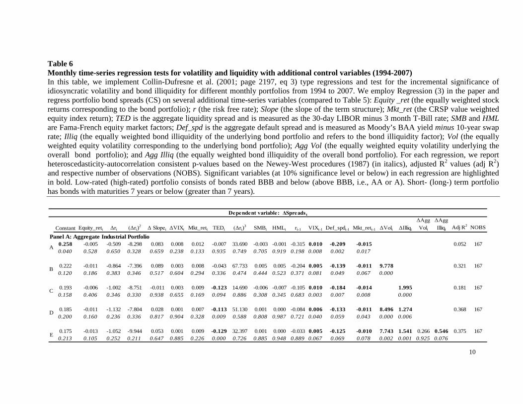
10
Table 6 Monthly time-series regression tests for volatility and liquidity with additional control variables (1994-2007) In this table, we implement Collin-Dufresne et al. (2001; page 2197, eq 3) type regressions and test for the incremental significance of idiosyncratic volatility and bond illiquidity for different monthly portfolios from 1994 to 2007. We employ Regression (3) in the paper and regress portfolio bond spreads (CS) on several additional time-series variables (compared to Table 5): Equity _ret (the equally weighted stock returns corresponding to the bond portfolio); r (the risk free rate); Slope (the slope of the term structure); Mkt_ret (the CRSP value weighted equity index return); TED is the aggregate liquidity spread and is measured as the 30-day LIBOR minus 3 month T-Bill rate; SMB and HML are Fama-French equity market factors; Def_spd is the aggregate default spread and is measured as Moody’s BAA yield minus 10-year swap rate; Illiq (the equally weighted bond illiquidity of the underlying bond portfolio and refers to the bond illiquidity factor); Vol (the equally weighted equity volatility corresponding to the underlying bond portfolio); Agg Vol (the equally weighted equity volatility underlying the overall bond portfolio); and Agg Illiq (the equally weighted bond illiquidity of the overall bond portfolio). For each regression, we report heteroscedasticity-autocorrelation consistent p-values based on the Newey-West procedures (1987) (in italics), adjusted R2 values (adj R2) and respective number of observations (NOBS). Significant variables (at 10% significance level or below) in each regression are highlighted in bold. Low-rated (high-rated) portfolio consists of bonds rated BBB and below (above BBB, i.e., AA or A). Short- (long-) term portfolio has bonds with maturities 7 years or below (greater than 7 years).
Constant Equity_rett Δrt (Δrt)2 Δ Slopet ΔVIXt Mkt_rett TEDt (Δrt)
3 SMBt HMLt rt-1 VIXt-1 Def_spdt-1 Mkt_rett-1 ΔVolt ΔIlliqt
ΔAgg Volt
ΔAgg Illiqt Adj R2 NOBS
0.258 -0.005 -0.509 -8.298 0.083 0.008 0.012 -0.007 33.690 -0.003 -0.001 -0.315 0.010 -0.209 -0.015 0.052 1670.040 0.528 0.650 0.328 0.659 0.238 0.133 0.935 0.749 0.705 0.919 0.198 0.008 0.002 0.017
0.222 -0.011 -0.864 -7.396 0.089 0.003 0.008 -0.043 67.733 0.005 0.005 -0.204 0.005 -0.139 -0.011 9.778 0.321 1670.120 0.186 0.383 0.346 0.517 0.604 0.294 0.336 0.474 0.444 0.523 0.371 0.081 0.049 0.067 0.000
0.193 -0.006 -1.002 -8.751 -0.011 0.003 0.009 -0.123 14.690 -0.006 -0.007 -0.105 0.010 -0.184 -0.014 1.995 0.181 1670.158 0.406 0.346 0.330 0.938 0.655 0.169 0.094 0.886 0.308 0.345 0.683 0.003 0.007 0.008 0.000
0.185 -0.011 -1.132 -7.804 0.028 0.001 0.007 -0.113 51.130 0.001 0.000 -0.084 0.006 -0.133 -0.011 8.496 1.274 0.368 1670.200 0.160 0.236 0.336 0.817 0.904 0.328 0.009 0.588 0.808 0.987 0.721 0.040 0.059 0.043 0.000 0.006
0.175 -0.013 -1.052 -9.944 0.053 0.001 0.009 -0.129 32.397 0.001 0.000 -0.033 0.005 -0.125 -0.010 7.743 1.541 0.266 0.546 0.375 1670.213 0.105 0.252 0.211 0.647 0.885 0.226 0.000 0.726 0.885 0.948 0.889 0.067 0.069 0.078 0.002 0.001 0.925 0.076
D
E
Dependent variable: ΔSpreads t
Panel A: Aggregate Industrial Portfolio
A
B
C

11
Constant Equity_rett Δrt (Δrt)2 Δ Slopet ΔVIXt Mkt_rett TEDt (Δrt)
3 SMBt HMLt rt-1 VIXt-1 Def_spdt-1 Mkt_rett-1 ΔVolt ΔIlliqt
ΔAgg Volt
ΔAgg Illiqt Adj R2 NOBS
0.094 0.002 -0.311 -0.876 0.057 -0.002 -0.002 0.046 4.268 -0.006 -0.004 -0.133 0.002 -0.063 -0.009 0.050 1670.100 0.743 0.533 0.860 0.557 0.525 0.694 0.231 0.930 0.117 0.252 0.121 0.238 0.027 0.009
0.085 0.001 -0.379 -1.492 0.049 -0.003 -0.002 0.043 5.168 -0.004 -0.002 -0.109 0.001 -0.054 -0.009 1.949 0.061 1670.129 0.836 0.448 0.772 0.601 0.457 0.743 0.273 0.917 0.228 0.394 0.196 0.410 0.054 0.007 0.060
0.089 0.001 -0.457 -1.890 0.049 -0.003 -0.002 0.047 5.511 -0.006 -0.003 -0.108 0.001 -0.058 -0.009 0.514 0.075 1670.116 0.784 0.342 0.693 0.600 0.405 0.747 0.206 0.908 0.100 0.341 0.172 0.366 0.049 0.005 0.007
0.081 0.001 -0.503 -2.330 0.042 -0.003 -0.001 0.044 6.173 -0.005 -0.002 -0.091 0.001 -0.050 -0.009 1.649 0.473 0.081 1670.141 0.864 0.298 0.638 0.637 0.364 0.787 0.243 0.899 0.176 0.476 0.251 0.521 0.078 0.004 0.107 0.011
0.084 0.000 -0.483 -2.532 0.075 -0.003 -0.001 0.044 9.331 -0.004 -0.001 -0.085 0.000 -0.043 -0.008 -0.022 0.537 2.113 0.199 0.115 1670.135 0.967 0.313 0.586 0.375 0.375 0.821 0.276 0.850 0.245 0.843 0.299 0.851 0.143 0.014 0.987 0.007 0.044 0.109
Constant Equity_rett Δrt (Δrt)2 Δ Slopet ΔVIXt Mkt_rett TEDt (Δrt)
3 SMBt HMLt rt-1 VIXt-1 Def_spdt-1 Mkt_rett-1 ΔVolt ΔIlliqt
ΔAgg Volt
ΔAgg Illiqt Adj R2 NOBS
0.238 -0.028 0.277 -12.051 0.056 0.018 0.035 -0.102 -20.043 -0.005 0.008 -0.100 0.009 -0.195 -0.021 0.058 1670.282 0.001 0.862 0.151 0.829 0.201 0.003 0.002 0.891 0.688 0.637 0.805 0.110 0.100 0.132
0.235 -0.032 -0.257 -7.083 0.135 0.012 0.026 -0.174 73.036 0.005 0.012 -0.068 0.006 -0.154 -0.012 8.982 0.258 1670.291 0.003 0.859 0.371 0.521 0.421 0.049 0.000 0.583 0.682 0.390 0.853 0.261 0.174 0.383 0.000
0.122 -0.030 0.216 -11.767 -0.048 0.014 0.032 -0.328 -80.057 -0.010 -0.004 0.213 0.011 -0.164 -0.015 2.742 0.148 1670.614 0.000 0.878 0.175 0.821 0.322 0.002 0.000 0.559 0.351 0.828 0.637 0.038 0.162 0.237 0.002
0.166 -0.032 -0.225 -7.548 0.062 0.010 0.026 -0.301 24.838 0.000 0.005 0.117 0.008 -0.140 -0.010 7.830 1.656 0.285 1670.470 0.002 0.870 0.330 0.761 0.487 0.041 0.000 0.849 0.993 0.748 0.765 0.149 0.206 0.453 0.000 0.034
0.160 -0.032 -0.277 -7.363 0.066 0.010 0.026 -0.291 34.170 0.002 0.008 0.124 0.007 -0.128 -0.010 6.601 1.588 3.585 -0.192 0.279 1670.478 0.004 0.841 0.365 0.756 0.476 0.045 0.000 0.784 0.822 0.510 0.749 0.219 0.223 0.429 0.005 0.064 0.429 0.750
A
B
C
D
E
A
B
C
D
E
Panel C: Low-rated Industrial Portfolio
Panel B: High-rated Industrial Portfolio
Dependent variable: ΔSpreads t
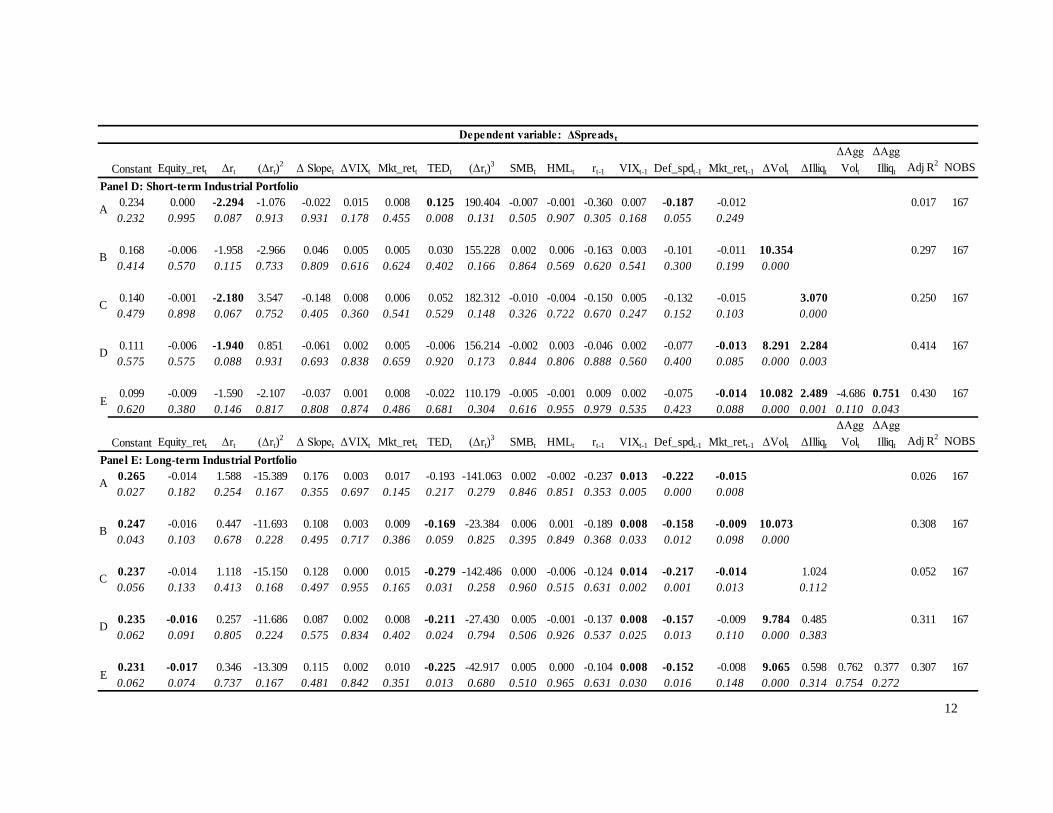
12
Constant Equity_rett Δrt (Δrt)2 Δ Slopet ΔVIXt Mkt_rett TEDt (Δrt)
3 SMBt HMLt rt-1 VIXt-1 Def_spdt-1 Mkt_rett-1 ΔVolt ΔIlliqt
ΔAgg Volt
ΔAgg Illiqt Adj R2 NOBS
0.234 0.000 -2.294 -1.076 -0.022 0.015 0.008 0.125 190.404 -0.007 -0.001 -0.360 0.007 -0.187 -0.012 0.017 1670.232 0.995 0.087 0.913 0.931 0.178 0.455 0.008 0.131 0.505 0.907 0.305 0.168 0.055 0.249
0.168 -0.006 -1.958 -2.966 0.046 0.005 0.005 0.030 155.228 0.002 0.006 -0.163 0.003 -0.101 -0.011 10.354 0.297 1670.414 0.570 0.115 0.733 0.809 0.616 0.624 0.402 0.166 0.864 0.569 0.620 0.541 0.300 0.199 0.000
0.140 -0.001 -2.180 3.547 -0.148 0.008 0.006 0.052 182.312 -0.010 -0.004 -0.150 0.005 -0.132 -0.015 3.070 0.250 1670.479 0.898 0.067 0.752 0.405 0.360 0.541 0.529 0.148 0.326 0.722 0.670 0.247 0.152 0.103 0.000
0.111 -0.006 -1.940 0.851 -0.061 0.002 0.005 -0.006 156.214 -0.002 0.003 -0.046 0.002 -0.077 -0.013 8.291 2.284 0.414 1670.575 0.575 0.088 0.931 0.693 0.838 0.659 0.920 0.173 0.844 0.806 0.888 0.560 0.400 0.085 0.000 0.003
0.099 -0.009 -1.590 -2.107 -0.037 0.001 0.008 -0.022 110.179 -0.005 -0.001 0.009 0.002 -0.075 -0.014 10.082 2.489 -4.686 0.751 0.430 1670.620 0.380 0.146 0.817 0.808 0.874 0.486 0.681 0.304 0.616 0.955 0.979 0.535 0.423 0.088 0.000 0.001 0.110 0.043
Constant Equity_rett Δrt (Δrt)2 Δ Slopet ΔVIXt Mkt_rett TEDt (Δrt)
3 SMBt HMLt rt-1 VIXt-1 Def_spdt-1 Mkt_rett-1 ΔVolt ΔIlliqt
ΔAgg Volt
ΔAgg Illiqt Adj R2 NOBS
0.265 -0.014 1.588 -15.389 0.176 0.003 0.017 -0.193 -141.063 0.002 -0.002 -0.237 0.013 -0.222 -0.015 0.026 1670.027 0.182 0.254 0.167 0.355 0.697 0.145 0.217 0.279 0.846 0.851 0.353 0.005 0.000 0.008
0.247 -0.016 0.447 -11.693 0.108 0.003 0.009 -0.169 -23.384 0.006 0.001 -0.189 0.008 -0.158 -0.009 10.073 0.308 1670.043 0.103 0.678 0.228 0.495 0.717 0.386 0.059 0.825 0.395 0.849 0.368 0.033 0.012 0.098 0.000
0.237 -0.014 1.118 -15.150 0.128 0.000 0.015 -0.279 -142.486 0.000 -0.006 -0.124 0.014 -0.217 -0.014 1.024 0.052 1670.056 0.133 0.413 0.168 0.497 0.955 0.165 0.031 0.258 0.960 0.515 0.631 0.002 0.001 0.013 0.112
0.235 -0.016 0.257 -11.686 0.087 0.002 0.008 -0.211 -27.430 0.005 -0.001 -0.137 0.008 -0.157 -0.009 9.784 0.485 0.311 1670.062 0.091 0.805 0.224 0.575 0.834 0.402 0.024 0.794 0.506 0.926 0.537 0.025 0.013 0.110 0.000 0.383
0.231 -0.017 0.346 -13.309 0.115 0.002 0.010 -0.225 -42.917 0.005 0.000 -0.104 0.008 -0.152 -0.008 9.065 0.598 0.762 0.377 0.307 1670.062 0.074 0.737 0.167 0.481 0.842 0.351 0.013 0.680 0.510 0.965 0.631 0.030 0.016 0.148 0.000 0.314 0.754 0.272
B
C
D
C
D
A
B
E
Panel D: Short-term Industrial Portfolio
Panel E: Long-term Industrial Portfolio
Dependent variable: ΔSpreads t
E
A

13
Table 7 Monthly Collin-Dufresne et al. (2001) time-series regression tests for volatility and liquidity for the extended sample (1994-2010) In this table, we implement Table 5 and 6 regressions for the full data sample and test for the incremental significance of idiosyncratic volatility and bond illiquidity for different monthly portfolios. For brevity, we report regression coefficients and corresponding Newey-West p-values only for idiosyncratic volatility and bond illiquidity variables, along with adjusted R2
values. Accordingly, Panel A reports Table 5 regressions (B, C, D, E, F and H), and Panel B reports Table 6 regressions (B, C, D and E), where NOBS for each regression is 203. Significant variables (at 10% significance level or below) in each regression are highlighted in bold. Low-rated (high-rated) portfolio consists of bonds rated BBB and below (above BBB, i.e., AA or A). Short- (long-) term portfolio has bonds with maturities 7 years or below (greater than 7 years).
ΔVolt-1 ΔLiqt Adj R2 ΔVolt-1 ΔLiqt Adj R2 ΔVolt-1 ΔLiqt Adj R2 ΔVolt-1 ΔLiqt Adj R2 ΔVolt-1 ΔLiqt Adj R2
B 12.966 0.326 2.813 0.233 13.211 0.349 15.428 0.301 16.123 0.4390.000 0.117 0.000 0.000 0.000
C 6.514 0.229 0.545 0.225 8.308 0.189 8.091 0.415 3.938 0.0460.000 0.078 0.003 0.000 0.049
D 10.700 4.585 0.421 2.815 0.545 0.241 11.314 5.037 0.401 11.477 6.747 0.570 15.834 0.600 0.4370.000 0.000 0.107 0.075 0.000 0.020 0.000 0.000 0.000 0.516
E 10.980 4.315 0.439 2.871 0.503 0.247 11.294 4.976 0.420 11.089 5.881 0.620 14.843 0.627 0.4750.000 0.005 0.106 0.092 0.000 0.024 0.000 0.000 0.000 0.501
F 10.760 3.519 0.455 2.856 0.450 0.241 11.435 4.616 0.446 11.502 6.422 0.626 16.308 0.516 0.5420.000 0.003 0.107 0.209 0.000 0.015 0.000 0.000 0.000 0.573
H 11.552 2.612 0.457 1.605 0.804 0.284 11.899 1.172 0.453 10.865 5.950 0.619 16.323 -2.739 0.5620.000 0.195 0.335 0.009 0.000 0.690 0.000 0.000 0.000 0.058
B 11.719 0.326 1.409 0.286 12.303 0.345 15.745 0.293 15.552 0.4270.000 0.350 0.000 0.000 0.000
C 6.361 0.318 0.533 0.294 7.702 0.245 7.969 0.424 3.919 0.1000.000 0.063 0.001 0.000 0.025
D 8.945 4.776 0.430 1.426 0.536 0.295 10.311 5.022 0.398 11.638 6.731 0.564 15.130 0.806 0.4270.000 0.000 0.330 0.060 0.001 0.015 0.000 0.000 0.000 0.380
E 9.310 4.622 0.429 0.651 0.598 0.314 10.606 4.682 0.398 11.117 7.017 0.594 16.293 -0.069 0.4660.000 0.000 0.629 0.052 0.001 0.042 0.000 0.000 0.000 0.933
Panel A: Table 5 regressions
Panel B: Table 6 regressions
Aggregate Industrial Portfolio
High-rated Industrial Portfolio
Low-rated Industrial Portfolio
Short-term Industrial Portfolio
Long-term Industrial Portfolio
14
Table 8 Monthly time-series regression tests with regime breaks for volatility and liquidity (1994-2010) In this table we report the monthly portfolio regression results with volatility and illiquidity regimes for different bond portfolios. We implement Regression (4) in the paper, or equivalently Regression E, Table 5, augmented with regime-specific dummies; i.e., we regress portfolio bond spreads (CS) on volatility and illiquidity, and corresponding low- and high-regime dummy variables (denoted respectively as Low- and High-Vol_reg and Low- and High-Illiq_reg). Regimes for each variable are identified using the Hamilton (1989) regime-switching model as depicted in Figure 4. For each regression, we report heteroscedasticity-autocorrelation consistent p-values based on the Newey-West procedures (1987) (in italics), adjusted R2 values (adj R2) and respective number of observations (NOBS). We highlight significant variables (at 10% significance level or below) in each regression in bold; in addition for each portfolio, we also highlight the regime that has a larger volatility or illiquidity coefficient. Low-rated (high-rated) portfolio consists of bonds rated BBB and below (above BBB, i.e., AA or A). Short- (long-) term portfolio has bonds with maturities 7 years or below (greater than 7 years).

15
Constant Equity_rett Δrt (Δrt)2 Δ Slopet ΔVIXt Mkt_rett
ΔVolt × Low-
Vol_reg
ΔVolt × High-
Vol_reg
ΔLiqt × Low-
Illiq_reg
ΔLiqt × High-
Illiq_reg ΔCSt-1 Adj R2 NOBS
0.014 0.001 -1.631 0.627 -0.425 0.003 -0.014 9.037 11.166 0.756 4.800 -0.142 0.443 2020.660 0.911 0.032 0.951 0.159 0.822 0.351 0.000 0.000 0.433 0.003 0.046
0.001 -0.002 -0.978 1.968 -0.155 0.021 0 1.617 3.820 0.433 0.462 -0.094 0.252 2020.958 0.804 0.027 0.682 0.069 0 0.948 0.427 0.038 0.169 0.269 0.106
0.014 0.003 -1.540 9.616 -0.804 0.001 -0.028 10.773 11.132 -0.181 5.684 -0.145 0.423 2020.774 0.862 0.187 0.581 0.091 0.977 0.309 0.000 0.002 0.890 0.015 0.036
0.018 -0.004 -0.818 -6.358 -0.203 0.032 -0.002 5.823 11.972 -0.817 6.865 -0.214 0.659 2020.548 0.827 0.281 0.426 0.427 0.043 0.909 0.002 0.000 0.058 0.000 0.017
0.027 -0.007 -1.267 0.017 -0.361 -0.013 -0.012 14.698 14.979 1.513 0.491 -0.211 0.470 2020.388 0.500 0.245 0.999 0.249 0.644 0.359 0.000 0.000 0.306 0.628 0.010
-0.004 -0.004 -1.344 4.368 -0.024 0.027 -0.001 0.630 2.172 0.646 -0.607 -0.304 0.206 2020.823 0.646 0.011 0.468 0.868 0.016 0.874 0.831 0.565 0.148 0.498 0.014
0.001 -0.009 -0.557 4.829 -0.159 0.017 0.004 1.067 2.708 0.170 0.422 -0.160 0.234 2020.940 0.190 0.165 0.310 0.078 0.000 0.474 0.495 0.178 0.780 0.131 0.005
-0.018 0.008 0.755 7.673 -0.391 0.052 -0.020 1.057 9.920 0.362 9.399 -0.166 0.537 2020.731 0.803 0.494 0.590 0.505 0.014 0.570 0.716 0.000 0.750 0.000 0.029
-0.010 0.005 -1.882 16.140 -1.169 -0.022 -0.045 5.701 11.471 1.192 2.768 -0.136 0.413 2020.843 0.738 0.247 0.483 0.045 0.615 0.045 0.143 0.000 0.537 0.124 0.179
High-rated Short-term Industrial Portfolio
High-rated Long-term Industrial Portfolio
Low-rated Short-term Industrial Portfolio
Low-rated Long-term Industrial Portfolio
Dependent variable: ΔSpreads t
Aggregate Industrial Portfolio
High-rated Industrial Portfolio
Low-rated Industrial Portfolio
Short-rated Industrial Portfolio
Long-rated Industrial Portfolio

16
Table 9 Granger casualty tests for monthly bond spreads, volatility and liquidity (1994-2010) In this table, we conduct Granger casualty tests to study the mutual lead-lag impact of bond spread, volatility and illiquidity variables. We report Chi-square tests and corresponding degrees of freedom (df) and p-values for the null of no-significance for each variable individually and jointly. The df accounting for the maximum number of lags for each variable is chosen based on the BIC selection criterion. We present three tables for each of the following monthly Industrial portfolios: Low-rated, Short-term and Low-rated/short-term. The first, second and third tables horizontally for each portfolio conduct Granger casualty tests respectively using changes in spreads, volatility and illiquidity as the dependent variables. In each panel, we highlight whenever a given variable (or a set of variables) is significant.
Chi-sq df P-value Chi-sq df P-value Chi-sq df P-value
ΔVolt 6.638 3 0.084 ΔSpreadt 35.931 3 0.000 ΔSpreadt 3.7361 3 0.291ΔIlliqt 8.716 3 0.033 ΔIlliqt 6.564 3 0.087 ΔVolt 3.1398 3 0.371
All 16.234 6 0.013 All 40.850 6 0.00 All 10.62 6 0.101
ΔVolt 5.966 3 0.093 ΔSpreadt 17.990 3 0.000 ΔSpreadt 4.0158 3 0.260ΔIlliqt 7.839 3 0.050 ΔIlliqt 5.746 3 0.125 ΔVolt 1.7957 3 0.616
All 15.001 6 0.020 All 21.154 6 0.002 All 7.5824 6 0.270
ΔVolt 19.207 3 0.000 ΔSpreadt 37.503 3 0.000 ΔSpreadt 7.5662 3 0.056ΔIlliqt 29.632 3 0.000 ΔIlliqt 16.950 3 0.001 ΔVolt 1.1219 3 0.772
All 48.572 6 0.000 All 49.658 6 0.000 All 16.282 6 0.012
Short-term Industrial Portfolio
Low-rated Short-term Industrial Portfolio
VAR Granger Causality/Block Exogeneity Wald Tests Dependent variable: ΔSpreadt Dependent variable: ΔVolt Dependent variable: ΔIlliqt
Low-rated Industrial Portfolio

17
Table 10 Generalized impulse response functions for monthly credit spread changes In this table we report accumulated responses of ΔBond Spreads to a generalized one sigma (or 1σ) innovation in each of three variables: ΔBond Spread, ΔIdiosyncratic Volatility and ΔBond Illiquidity. We present the accumulated impulse responses up to 10 periods ahead and the corresponding p-values (in italics) for Low-rated, Short-term and Low-rated/short-term Industrial portfolios, based on the monthly VAR model (5). Panel A reports the results for the pre-crisis or 1994-2007 period and Panel B for the 1994-2010 period. Significant responses (at 10% significance level or below) in each regression are highlighted in bold. Low-rated portfolio consists of bonds rated BBB and below. Short-term portfolio has bonds with maturities 7 years or below.
Period ΔSpreadt ΔVol t ΔIlliqt ΔSpreadt ΔVol t ΔIlliqt ΔSpreadt ΔVol t ΔIlliqt
1 0.490 0.230 0.110 0.390 0.200 0.170 0.660 0.320 0.2200.000 0.000 -0.002 0.000 0.000 0.000 0.000 0.000 0.000
2 0.300 0.040 -0.050 0.260 0.090 0.020 0.460 0.130 -0.0800.000 -0.340 -0.317 0.000 -0.021 -0.677 0.000 -0.060 -0.269
3 0.230 0.020 -0.060 0.220 0.000 0.000 0.380 0.030 -0.050
0.000 -0.654 -0.249 0.000 -0.996 -0.977 0.000 -0.665 -0.5394 0.260 0.090 -0.040 0.230 0.100 0.020 0.380 0.170 -0.050
0.000 -0.085 -0.407 0.000 -0.034 -0.616 0.000 -0.045 -0.4815 0.260 0.070 0.010 0.240 0.060 0.080 0.390 0.130 0.050
0.000 -0.099 -0.649 0.000 -0.240 -0.005 0.000 -0.098 -0.3636 0.270 0.070 -0.020 0.210 0.030 0.030 0.390 0.100 -0.040
0.000 -0.096 -0.550 0.000 -0.518 -0.252 0.000 -0.208 -0.4857 0.270 0.070 -0.030 0.240 0.080 0.030 0.410 0.150 0.010
0.000 -0.099 -0.499 0.000 -0.092 -0.296 0.000 -0.052 -0.8668 0.260 0.070 -0.020 0.230 0.060 0.040 0.390 0.120 -0.020
0.000 -0.095 -0.519 0.000 -0.181 -0.246 0.000 -0.099 -0.6689 0.260 0.070 -0.020 0.230 0.050 0.040 0.390 0.110 -0.010
0.000 -0.095 -0.616 0.000 -0.312 -0.105 0.000 -0.091 -0.84510 0.270 0.070 -0.020 0.230 0.070 0.040 0.400 0.140 -0.010
0.000 -0.097 -0.579 0.000 -0.098 -0.150 0.000 -0.075 -0.897
Panel A: Accumulated Impulse Response Functions for ΔBond Spreads (1994-2007)
Industrials Low-rated Industrials Short-termIndustrials Low-rated
Short-term

18
Period ΔSpreadt ΔVol t ΔIlliqt ΔSpreadt ΔVol t ΔIlliqt ΔSpreadt ΔVol t ΔIlliqt
1 1.135 0.766 0.452 0.934 0.535 0.431 1.414 0.881 0.5370.000 0.000 0.000 0.000 0.000 0.000 0.000 0.000 0.000
2 1.028 0.778 0.281 0.549 0.258 0.114 1.211 0.673 0.0930.000 0.000 0.015 0.000 0.002 0.164 0.000 0.000 0.553
3 1.062 0.811 0.424 0.707 0.509 0.180 1.183 0.837 0.422
0.000 0.000 0.002 0.000 0.000 0.057 0.000 0.000 0.0094 1.116 0.723 0.200 0.774 0.460 0.169 1.108 0.474 0.064
0.000 0.000 0.235 0.000 0.000 0.108 0.000 0.011 0.7315 1.139 0.776 0.220 0.761 0.481 0.274 1.100 0.621 0.270
0.000 0.000 0.068 0.000 0.000 0.001 0.000 0.000 0.1026 1.115 0.794 0.249 0.789 0.505 0.246 1.062 0.604 0.240
0.000 0.000 0.051 0.000 0.000 0.009 0.000 0.000 0.1227 1.053 0.727 0.250 0.763 0.474 0.226 0.978 0.504 0.112
0.000 0.000 0.056 0.000 0.000 0.014 0.000 0.003 0.4428 1.084 0.738 0.252 0.791 0.507 0.240 1.106 0.629 0.285
0.000 0.000 0.053 0.000 0.000 0.008 0.000 0.000 0.0759 1.090 0.754 0.240 0.780 0.491 0.180 1.049 0.567 0.175
0.000 0.000 0.053 0.000 0.000 0.045 0.000 0.000 0.22010 1.078 0.756 0.220 0.784 0.499 0.171 1.049 0.591 0.220
0.000 0.000 0.077 0.000 0.000 0.060 0.000 0.000 0.103
Panel B: Accumulated Impulse Response Functions for ΔBond Spreads (1994-2010)
Industrials Low-rated Industrials Short-termIndustrials Low-rated
Short-term

19
Table 11 Cholesky variance decomposition of volatility and liquidity effects on bond spreads (1994-2010) In this table, we conduct Cholesky variance decomposition to study the impact of volatility and illiquidity variables on the variance of the residual bond spreads. We consider two different orderings of the volatility and illiquidity variables. For Ordering 1, we employ the following residual regression to obtain the variance shares:
( )
( )t10,1
17
t6t5t42
32t10t
t2,110t
and
Res
where, Res
IlliqVoleCS
Mkt_retVIXSloperrEquity_retCS
Illiqe
tt
t
ttt
tt
∆+−∆=
∆+
+∆+∆+∆+∆++−∆=
+∆++=
−
γγ
β
βββββββ
ηααα
The variance share explained by volatility is obtained as : )Resvar()var( t,11 teα , and the variance share explained by illiquidity as: )Resvar()var( t2 tIlliq∆α . Next for Ordering 2, we reorder the volatility and illiquidity variables and define the residual equation as before as obtained is Res where Res tt,2210t ηααα ++∆+= tteVol
( )t10,2 and VolIlliqe tt ∆+−∆= γγ . We obtain the variance shares for the pre-crisis and overall periods (Panel A) and separately for the low- and high- credit spread, volatility and illiquidity regimes (Panel B). The low- and high- regimes are identified using the two-state Hamilton (1989) model as in Figure 4 and explained under Table 8. For each ordering, we highlight whichever variable has a higher variance share. Panel A: Information shares for volatility and illiquidity for the pre-crisis and overall periods
ΔVolt ΔIlliqt ΔVolt ΔIlliqt ΔVolt ΔIlliqt ΔVolt ΔIlliqt
Aggregate Industrial Portfolio Aggregate Industrial Portfolio0.187 0.113 0.265 0.035 0.199 0.200 0.316 0.083
High-rated Industrial Portfolio High-rated Industrial Portfolio0.024 0.014 0.029 0.009 0.025 0.013 0.026 0.012
Low-rated Industrial Portfolio Low-rated Industrial Portfolio0.144 0.093 0.208 0.029 0.204 0.171 0.320 0.055
Short-term Industrial Portfolio Short-term Industrial Portfolio0.165 0.189 0.269 0.086 0.167 0.317 0.284 0.200
Long-term Industrial Portfolio Long-term Industrial Portfolio0.224 0.025 0.246 0.004 0.325 0.055 0.377 0.002
Ordering 1 Ordering 2
1994-97
Ordering 1 Ordering 2
1994-2010

20
Panel B: Information shares for volatility and illiquidity for high and low regimes (1994-2010)
Ordering 1 Ordering 2 Ordering 1 Ordering 2ΔVolt ΔIlliqt ΔVolt ΔIlliqt ΔVolt ΔIlliqt ΔVolt ΔIlliqt
Aggregate Industrial Portfolio0.062 0.061 0.085 0.038 0.203 0.230 0.340 0.093
High-rated Industrial Portfolio0.036 0.046 0.047 0.035 0.022 0.005 0.021 0.005
Low-rated Industrial Portfolio0.029 0.051 0.040 0.040 0.210 0.195 0.347 0.058
Short-term Industrial Portfolio0.038 0.072 0.065 0.045 0.169 0.363 0.300 0.232
Long-term Industrial Portfolio0.126 0.015 0.122 0.019 0.343 0.065 0.408 0
ΔVolt ΔIlliqt ΔVolt ΔIlliqt ΔVolt ΔIlliqt ΔVolt ΔIlliqt
Aggregate Industrial Portfolio0.235 0.145 0.347 0.033 0.188 0.225 0.313 0.100
High-rated Industrial Portfolio0.049 0.028 0.052 0.025 0.020 0.008 0.020 0.007
Low-rated Industrial Portfolio0.200 0.085 0.266 0.019 0.183 0.215 0.326 0.073
Short-term Industrial Portfolio0.176 0.145 0.256 0.064 0.16 0.362 0.287 0.235
Long-term Industrial Portfolio0.322 0.015 0.334 0.003 0.309 0.075 0.382 0.002
ΔVolt ΔIlliqt ΔVolt ΔIlliqt ΔVolt ΔLiqt ΔVolt ΔIlliqt
Aggregate Industrial Portfolio0.081 0.004 0.084 0.001 0.199 0.230 0.333 0.096
High-rated Industrial Portfolio0.035 0.022 0.043 0.013 0.024 0.011 0.023 0.012
Low-rated Industrial Portfolio0.032 0.001 0.033 0 0.206 0.196 0.340 0.062
Short-term Industrial Portfolio0.095 0 0.089 0.006 0.164 0.364 0.293 0.236
Long-term Industrial Portfolio0.129 0.001 0.129 0 0.335 0.066 0.399 0.001
HIGH REGIMELOW REGIMECREDIT SPREAD REGIMES
VOLATILTIY BASED REGIMESLOW REGIME HIGH REGIME
Ordering 1 Ordering 2 Ordering 1 Ordering 2
IllIQUIDITY BASED REGIMESLOW REGIME HIGH REGIME
Ordering 1 Ordering 2 Ordering 1 Ordering 2
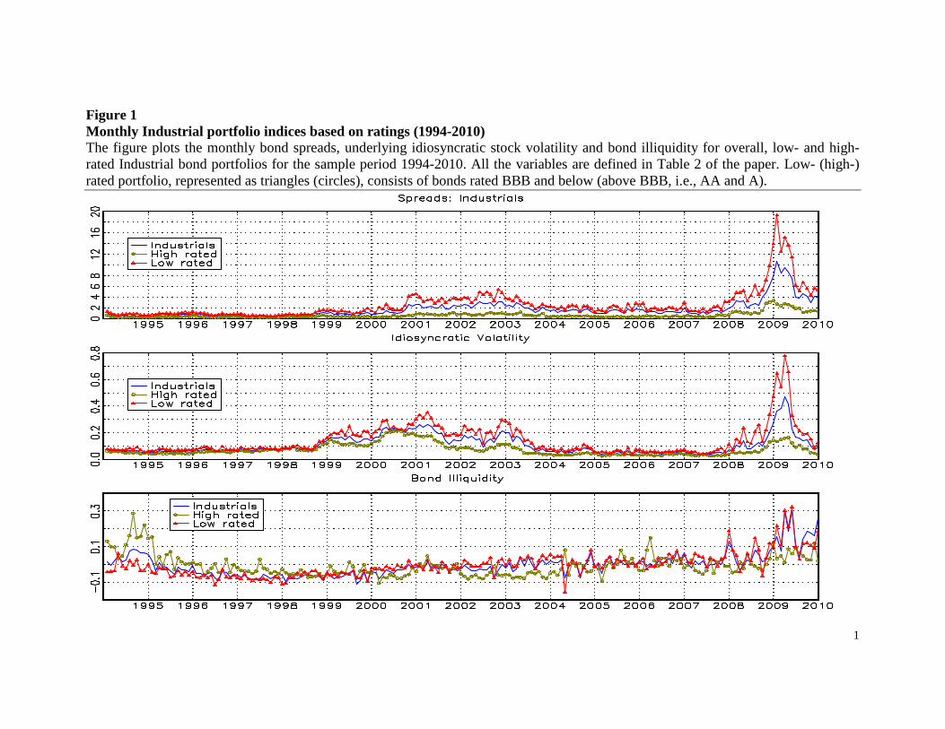
1
Figure 1 Monthly Industrial portfolio indices based on ratings (1994-2010) The figure plots the monthly bond spreads, underlying idiosyncratic stock volatility and bond illiquidity for overall, low- and high-rated Industrial bond portfolios for the sample period 1994-2010. All the variables are defined in Table 2 of the paper. Low- (high-) rated portfolio, represented as triangles (circles), consists of bonds rated BBB and below (above BBB, i.e., AA and A).

2
Figure 2 Monthly Industrial portfolio indices based on maturity (1994-2010) The figure plots the monthly bond spreads, underlying idiosyncratic stock volatility and bond illiquidity for overall, short- and long-term Industrial bond portfolios for the sample period 1994-2010. All the variables are defined in Table 2 of the paper. Short- (long-) term portfolio, represented as triangles (circles), consists of bonds with maturities 7 years or below (greater than 7 years).
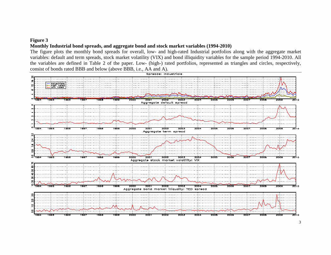
3
Figure 3 Monthly Industrial bond spreads, and aggregate bond and stock market variables (1994-2010) The figure plots the monthly bond spreads for overall, low- and high-rated Industrial portfolios along with the aggregate market variables: default and term spreads, stock market volatility (VIX) and bond illiquidity variables for the sample period 1994-2010. All the variables are defined in Table 2 of the paper. Low- (high-) rated portfolios, represented as triangles and circles, respectively, consist of bonds rated BBB and below (above BBB, i.e., AA and A).

4
Figure 4 Underlying regimes in monthly Industrial bond spreads idiosyncratic volatility and bond liquidity (1994-2010) The figure plots the Markov switching regimes based on the two-state Hamilton (1989) model for different monthly Industrial portfolios for bond spread, idiosyncratic volatility and bond illiquidity variables for the period 1994-2010.
Industrials Low-rated Portfolio
Industrials Short-term Portfolio
Industrials Low-rated Short-term Portfolio
0
5
10
15
20
94 95 96 97 98 99 00 01 02 03 04 05 06 07 08 09 10
Spreads
0.00
0.15
0.30
0.45
0.60
0.75
94 95 96 97 98 99 00 01 02 03 04 05 06 07 08 09 10
Volatility
-0.2
-0.1
0
0.1
0.2
0.3
0.4
94 95 96 97 98 99 00 01 02 03 04 05 06 07 08 09 10
Illiquidity
0
2
4
6
8
10
94 95 96 97 98 99 00 01 02 03 04 05 06 07 08 09 10
Spreads
0.00
0.15
0.30
0.45
94 95 96 97 98 99 00 01 02 03 04 05 06 07 08 09 10
Volatility
-0.2
-0.1
0
0.1
0.2
0.3
94 95 96 97 98 99 00 01 02 03 04 05 06 07 08 09 10
Illiquidity
0
5
10
15
20
94 95 96 97 98 99 00 01 02 03 04 05 06 07 08 09 10
Spreads
0.00
0.15
0.30
0.45
0.60
0.75
0.90
94 95 96 97 98 99 00 01 02 03 04 05 06 07 08 09 10
Volatility
-0.2
-0.1
0
0.1
0.2
94 95 96 97 98 99 00 01 02 03 04 05 06 07 08 09 10
Illiquidity
5
Figure 5 Generalized impulse response functions for monthly credit spread changes We plot the accumulated responses of ΔBond Spreads to a generalized one sigma (or 1σ) innovation (solid line) in each of the three variables, ΔBond Spread, ΔIdiosyncratic Volatility and ΔBond Illiquidity, using the monthly VAR model (5) for both the 1994-2007 (Panel A) and 1994-2010 (Panel B) periods. We also plot the response confidence bands for 90% (dotted) and 95% (dashed) confidence levels. We present three plots for each of the Low-rated, Short-term and Low-rated/short-term Industrial portfolios. The first plot under each portfolio refers to the accumulated response of ΔBond Spread to 1σ shock in Bond Spread. The second plot refers to the accumulated response of ΔBond Spreads to 1σ shock in Idiosyncratic Volatility. The third plot refers to the accumulated response of ΔBond Spread to 1σ shock in Bond Illiquidity. Low-rated portfolio consists of bonds rated BBB and below. Short-term portfolio has bonds with maturities 7 years or below.

6
Panel A: 1994-2007 sub-sample
Industrials Low-rated Industrials Short-term Industrials Low-rated Short-term
-0.2
0.0
0.2
0.4
0.6
1 2 3 4 5 6 7 8 9 10
ΔSpreads to ΔSpreads
-0.2
0.0
0.2
0.4
0.6
1 2 3 4 5 6 7 8 9 10
ΔSpreads to ΔSpreads
-0.2
0.0
0.2
0.4
0.6
1 2 3 4 5 6 7 8 9 10
ΔSpreads to ΔSpreads
-0.2
0.0
0.2
0.4
0.6
1 2 3 4 5 6 7 8 9 10
ΔSpreads to ΔVolatility
-0.2
0.0
0.2
0.4
0.6
1 2 3 4 5 6 7 8 9 10
ΔSpreads to ΔVolatility
-0.2
0.0
0.2
0.4
0.6
1 2 3 4 5 6 7 8 9 10
ΔSpreads to ΔVolatility
-0.2
0.0
0.2
0.4
0.6
1 2 3 4 5 6 7 8 9 10
ΔSpreads to ΔLiquidity
-0.2
0.0
0.2
0.4
0.6
1 2 3 4 5 6 7 8 9 10
ΔSpreads to ΔLiquidity
-0.2
0.0
0.2
0.4
0.6
1 2 3 4 5 6 7 8 9 10
ΔSpreads to ΔLiquidity
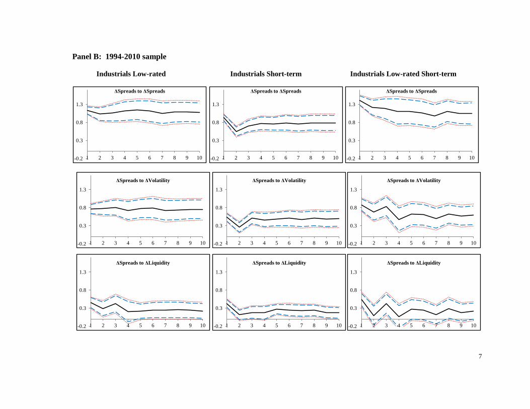
7
Panel B: 1994-2010 sample Industrials Low-rated Industrials Short-term Industrials Low-rated Short-term
-0.2
0.3
0.8
1.3
1 2 3 4 5 6 7 8 9 10
ΔSpreads to ΔSpreads
-0.2
0.3
0.8
1.3
1 2 3 4 5 6 7 8 9 10
ΔSpreads to ΔSpreads
-0.2
0.3
0.8
1.3
1 2 3 4 5 6 7 8 9 10
ΔSpreads to ΔSpreads
-0.2
0.3
0.8
1.3
1 2 3 4 5 6 7 8 9 10
ΔSpreads to ΔVolatility
-0.2
0.3
0.8
1.3
1 2 3 4 5 6 7 8 9 10
ΔSpreads to ΔVolatility
-0.2
0.3
0.8
1.3
1 2 3 4 5 6 7 8 9 10
ΔSpreads to ΔVolatility
-0.2
0.3
0.8
1.3
1 2 3 4 5 6 7 8 9 10
ΔSpreads to ΔLiquidity
-0.2
0.3
0.8
1.3
1 2 3 4 5 6 7 8 9 10
ΔSpreads to ΔLiquidity
-0.2
0.3
0.8
1.3
1 2 3 4 5 6 7 8 9 10
ΔSpreads to ΔLiquidity