Dynamic Dataflow Graphs - Electronic Systems
40
Dynamic Dataflow Graphs Shuvra S. Bhattacharyya, Ed F. Deprettere, and Bart D. Theelen Abstract Much of the work to date on dataflow models for signal processing system design has focused on decidable dataflow models that are best suited for one-dimensional signal processing. This chapter reviews more general dataflow modeling techniques that are targeted to applications that include multidimensional signal processing and dynamic dataflow behavior. As dataflow techniques are applied to signal processing systems that are more complex, and demand increasing degrees of agility and flexibility, these classes of more general dataflow models are of correspondingly increasing interest. We first provide a motivation for dynamic dataflow models of computation, and review a number of specific methods that have emerged in this class of models. Our coverage of dynamic dataflow models in this chapter includes Boolean dataflow, CAL, parameterized dataflow, enable- invoke dataflow, dynamic polyhedral process networks, scenario aware dataflow, and a stream-based function actor model. 1 Motivation for Dynamic DSP-Oriented Dataflow Models The decidable dataflow models covered in [31] are useful for their predictability, strong formal properties, and amenability to powerful optimization techniques. However, for many signal processing applications, it is not possible to represent S.S. Bhattacharyya () University of Maryland, College Park, MD, USA e-mail: [email protected] E.F. Deprettere Leiden University, Leiden, The Netherlands e-mail: [email protected] B.D. Theelen Embedded Systems Innovation by TNO, Eindhoven, The Netherlands e-mail: [email protected] S.S. Bhattacharyya et al. (eds.), Handbook of Signal Processing Systems, DOI 10.1007/978-1-4614-6859-2 28, © Springer Science+Business Media, LLC 2013 905
Transcript of Dynamic Dataflow Graphs - Electronic Systems

Dynamic Dataflow Graphs
Shuvra S. Bhattacharyya, Ed F. Deprettere, and Bart D. Theelen
Abstract Much of the work to date on dataflow models for signal processingsystem design has focused on decidable dataflow models that are best suited forone-dimensional signal processing. This chapter reviews more general dataflowmodeling techniques that are targeted to applications that include multidimensionalsignal processing and dynamic dataflow behavior. As dataflow techniques areapplied to signal processing systems that are more complex, and demand increasingdegrees of agility and flexibility, these classes of more general dataflow models areof correspondingly increasing interest. We first provide a motivation for dynamicdataflow models of computation, and review a number of specific methods thathave emerged in this class of models. Our coverage of dynamic dataflow modelsin this chapter includes Boolean dataflow, CAL, parameterized dataflow, enable-invoke dataflow, dynamic polyhedral process networks, scenario aware dataflow,and a stream-based function actor model.
1 Motivation for Dynamic DSP-Oriented Dataflow Models
The decidable dataflow models covered in [31] are useful for their predictability,strong formal properties, and amenability to powerful optimization techniques.However, for many signal processing applications, it is not possible to represent
S.S. Bhattacharyya (�)University of Maryland, College Park, MD, USAe-mail: [email protected]
E.F. DeprettereLeiden University, Leiden, The Netherlandse-mail: [email protected]
B.D. TheelenEmbedded Systems Innovation by TNO, Eindhoven, The Netherlandse-mail: [email protected]
S.S. Bhattacharyya et al. (eds.), Handbook of Signal Processing Systems,DOI 10.1007/978-1-4614-6859-2 28, © Springer Science+Business Media, LLC 2013
905

906 S.S. Bhattacharyya et al.
all of the functionality in terms of purely decidable dataflow representations. Forexample, functionality that involves conditional execution of dataflow subsystems oractors with dynamically varying production and consumption rates generally cannotbe expressed in decidable dataflow models.
The need for expressive power beyond that provided by decidable dataflowtechniques is becoming increasingly important in design and implementation signalprocessing systems. This is due to the increasing levels of application dynamicsthat must be supported in such systems, such as the need to support multi-standardand other forms of multi-mode signal processing operation; variable data rateprocessing; and complex forms of adaptive signal processing behaviors.
Intuitively, dynamic dataflow models can be viewed as dataflow modelingtechniques in which the production and consumption rates of actors can vary inways that are not entirely predictable at compile time. It is possible to definedynamic dataflow modeling formats that are decidable. For example, by restrictingthe types of dynamic dataflow actors, and by restricting the usage of such actors toa small set of graph patterns or “schemas”, Gao, Govindarajan, and Panangadendefined the class of well-behaved dataflow graphs, which provides a dynamicdataflow modeling environment that is amenable to compile-time bounded memoryverification [19].
However, most existing DSP-oriented dynamic dataflow modeling techniques donot provide decidable dataflow modeling capabilities. In other words, in exchangefor the increased modeling flexibility (expressive power) provided by such tech-niques, one must typically give up guarantees on compile-time buffer underflow(deadlock) and overflow validation. In dynamic dataflow environments, analysistechniques may succeed in guaranteeing avoidance of buffer underflow and overflowfor a significant subset of specifications, but, in general, specifications may arisethat “break” these analysis techniques—i.e., that result in inconclusive results fromcompile-time analysis.
Dynamic dataflow techniques can be divided into two general classes: (1) thosethat are formulated explicitly in terms of interacting combinations of state machinesand dataflow graphs, where the dataflow dynamics are represented directly in termsof transitions within one or more underlying state machines; and (2) those wherethe dataflow dynamics are represented using alternative means. The separation inthis dichotomy can become somewhat blurry for models that have a well-definedstate structure governing the dataflow dynamics, but whose design interface doesnot expose this structure directly to the programmer. Dynamic dataflow techniquesin the first category described above are covered in [31]—in particular, those basedon explicit interactions between dataflow graphs and finite state machines. Thischapter focusses on the second category.1 Specifically, dynamic dataflow modelingtechniques that involve different kinds of modeling abstractions, apart from statetransitions, as the key mechanisms for capturing dataflow behaviors and theirpotential for run-time variation.
1Except for the Scenario Aware Dataflow model in Sect. 6.
Dynamic Dataflow Graphs 907
Numerous dynamic dataflow modeling techniques have evolved over the pastcouple of decades. A comprehensive coverage of these techniques, even afterexcluding the “state-centric” ones, is out of the scope this chapter. The objective isto provide a representative cross-section of relevant dynamic dataflow techniques,with emphasis on techniques for which useful forms of compile time analysis havebeen developed. Such techniques can be important for exploiting the specializedproperties exposed by these models, and improving predictability and efficiencywhen deriving simulations or implementations.
2 Boolean Dataflow
The Boolean dataflow (BDF) model of computation extends synchronous dataflowwith a class of dynamic dataflow actors in which production and consumptionrates on actor ports can vary as two-valued functions of control tokens, which areconsumed from or produced onto designated control ports of dynamic dataflowactors. An actor input port is referred to as a conditional input port if its consumptionrate can vary in such a way, and similarly an output port with a dynamically varyingproduction rate under this model is referred to as a conditional output port.
Given a conditional input port p of a BDF actor A, there is a correspondinginput port Cp, called the control input for p, such that the consumption rate on Cp isstatically fixed at one token per invocation of A, and the number of tokens consumedfrom p during a given invocation of A is a two-valued function of the data value thatis consumed from Cp during the same invocation.
The dynamic dataflow behavior for a conditional output port is characterized in asimilar way, except that the number of tokens produced on such a port can be a two-valued function of a token that is consumed from a control input port or of a tokenthat is produced onto a control output port. If a conditional output port q is controlledby a control output port Cq, then the production rate on the control output is staticallyfixed at one token per actor invocation, and the number of tokens produced on qduring a given invocation of the enclosing actor is a two-valued function of the datavalue that is produced onto Cq during the same invocation of the actor.
Two fundamental dynamic dataflow actors in BDF are the switch and selectactors, which are illustrated in Fig. 1a. The switch actor has two input ports, a controlinput port wc and a data input port wd , and two output ports wx and wy. The port wc
accepts Boolean valued tokens, and the consumption rate on wd is statically fixedat one token per actor invocation. On a given invocation of a switch actor, the datavalue consumed from wd is copied to a token that is produced on either wx or wy
depending on the Boolean value consumed from wc. If this Boolean value is true,then the value from the data input is routed to wx, and no token is produced on wy.Conversely if the control token value is false, then the value from wd is routed towy with no token produced on wx.

908 S.S. Bhattacharyya et al.
Switch and Select If-then-else
a b
Fig. 1 (a) Switch and select actors in Boolean dataflow, and (b) an if-then-else construct expressedin terms of Boolean dataflow
A BDF select actor has a single control input port sc; two additional input ports(data input ports) sx and sy; and a single output port so. Similar to the control port ofthe switch actor, the sc port accepts Boolean valued tokens, and the production rateon the so port is statically fixed at one token per invocation. On each invocation ofthe select actor data is copied from a single token from either sx or sy to so dependingon whether the corresponding control token value is true or false respectively.
Switch and select actors can be integrated along with other actors in various waysto express different kinds of control constructs. For example, Fig. 1b illustrates anif-then-else construct, where the actors A and B are applied conditionally based on astream of control tokens. Here A and B are synchronous dataflow (SDF) actors thateach consume one token and produce one token on each invocation.
Buck has developed scheduling techniques to automatically derive efficientcontrol structures from BDF graphs under certain conditions [11]. Buck has alsoshown that BDF is Turing complete, and furthermore, that SDF augmented with justswitch and select (and no other dynamic dataflow actors) is also Turing complete.This latter result provides a convenient framework with which one can demonstrateTuring completeness for other kinds of dynamic dataflow models, such as theenable-invoke dataflow model described in Sect. 5. In particular, if a given modelof computation can express all SDF actors as well as the functionality associatedwith the BDF switch and select actors, then such a model can be shown to be Turingcomplete.
Dynamic Dataflow Graphs 909
3 CAL
In addition to providing a dynamic dataflow model of computation that is suitablefor signal processing system design, CAL provides a complete programminglanguage and is supported by a growing family of development tools for hardwareand software implementation. The name “CAL” is derived as a self-referentialacronym for the CAL actor language. CAL was developed by Eker and Janneckat U.C. Berkeley [14], and has since evolved into an actively-developed, widely-investigated language for design and implementation of embedded software andfield programmable gate array applications (e.g., see [30, 56, 77]). One of the mostnotable developments to date in the evolution of CAL has been its adoption as partof the recent MPEG standard for reconfigurable video coding (RVC) [8].
A CAL program is specified as a network of CAL actors, where each actor isa dataflow component that is expressed in terms of a general underlying form ofdataflow. This general form of dataflow admits both static and dynamic behaviors,and even non-deterministic behaviors.
Like typical actors in any dataflow programming environment, a CAL actor ingeneral has a set of input ports and a set of output ports that define interfaces tothe enclosing dataflow graph. A CAL actor also encapsulates its own private state,which can be modified by the actor as it executes but cannot be modified directly byother actors.
The functional specification of a CAL actor is decomposed into a set of actions,where each action can be viewed as a template for a specific class of firings orinvocations of the actor. Each firing of an actor corresponds to a specific action andexecutes based on the code that is associated with that action. The core functionalityof actors therefore is embedded within the code of the actions. Actions can ingeneral consume tokens from actor input ports, produce tokens on output ports,modify the actor state, and perform computation in terms of the actor state and thedata obtained from any consumed tokens.
The number of tokens produced and consumed by each action with respect toeach actor output and input port, respectively, is declared up front as part of thedeclaration of the action. An action need not consume data from all input ports normust it produce data on all output ports, but ports with which the action exchangesdata, and the associated rates of production and consumption must be constant forthe action. Across different actions, however, there is no restriction of uniformityin production and consumption rates, and this flexibility enables the modeling ofdynamic dataflow in CAL.
A CAL actor A can be represented as a sequence of four elements
σ0(A),Σ(A),Γ (A),pri(A), (1)
where Σ(A) represents the set of all possible values that the state of A can takeon; σ0(A) ∈ Σ(A) represents the initial state of the actor, before any actor in theenclosing dataflow graph has started execution; Γ (A) represents the set of actionsof A; and pri(A) is a partial order relation, called the priority relation of A, on Γ (A)that specifies relative priorities between actions.

910 S.S. Bhattacharyya et al.
Actions execute based on associated guard conditions as well as the priorityrelation of the enclosing actor. More specifically, each actor has an associated guardcondition, which can be viewed as a Boolean expression in terms of the values ofactor input tokens and actor state. An actor A can execute whenever its associatedguard condition is satisfied (true-valued), and no higher-priority action (based onthe priority relation pri(A)) has a guard condition that is also satisfied.
In summary, CAL is a language for describing dataflow actors in terms ofports, actions (firing templates), guards, priorities, and state. This finer, intra-actorgranularity of formal modeling within CAL allows for novel forms of automatedanalysis for extracting restricted forms of dataflow structure. Such restricted formsof structure can be exploited with specialized techniques for verification or synthesisto derive more predictable or efficient implementations.
An example of this capability for specialized region detection in CAL programsis the technique of deriving and exploiting so-called statically schedulable regions(SSRs) [30]. Intuitively, an SSR is a collection of CAL actions and ports that can bescheduled and optimized statically using the full power of static dataflow techniques,such as those available for SDF, and integrated into the schedule for the overall CALprogram through a top-level dynamic scheduling interface.
SSRs can be derived through a series of transformations that are applied on inter-mediate graph representations. These representations capture detailed relationshipsamong actor ports and actions, and provide a framework for effective quasi-static scheduling of CAL-based dynamic dataflow representations. Quasi-staticscheduling is the construction of dataflow graph schedules in which a significantproportion of overall schedule structure is fixed at compile-time. Quasi-staticscheduling has the potential to significantly improve predictability, reduce run-timescheduling overhead, and as discussed above, expose subsystems whose internalschedules can be generated using purely static dataflow scheduling techniques.
Further discussion about CAL can be found in [42], which discusses theapplication of CAL to reconfigurable video coding.
4 Parameterized Dataflow
Parameterized dataflow is a meta-modeling approach for integrating dynamicparameters and run-time adaptation of parameters in a structured way into a certainclass of dataflow models of computations, in particular, those models that have awell-defined concept of a graph iteration [6]. For example, SDF and cycle-staticSDF (CSDF), which are discussed in [31], and multidimensional SDF (MDSDF),which is discussed in [37], have well defined concepts of iterations based onsolutions to the associated forms of balance equations. Each of these models can beintegrated with parameterized dataflow to provide a dynamically parameterizableform of the original model.
When parameterized dataflow is applied in this way to generalize a specializeddataflow model such as SDF, CSDF, or MDSDF, the specialized model is referred

Dynamic Dataflow Graphs 911
to as the base model, and the resulting, dynamically parameterizable form ofthe base model is referred to as parameterized XYZ, where XYZ is the name ofthe base model. For example, when parameterized dataflow is applied to SDFas the base model, the resulting model of computation, called parameterizedsynchronous dataflow (PSDF), is significantly more flexible than SDF as it allowsarbitrary parameters of SDF graphs to be modified at run-time. Furthermore,PSDF provides a useful framework for quasi-static scheduling, where fixed-iterationlooped schedules, such as single appearance schedules [7], for SDF graphs can bereplaced by parameterized looped schedules [6, 40] in which loop iteration countsare represented as symbolic expressions in terms of variables whose values canbe adapted dynamically through computations that are derived from the enclosingPSDF specification.
Intuitively, parameterized dataflow allows arbitrary attributes of a dataflow graphto be parameterized, with each parameter characterized by an associated domain ofadmissible values that the parameter can take on at any given time. Graph attributesthat can be parameterized include scalar or vector attributes of individual actors,such as the coefficients of a finite impulse response filter or the block size associatedwith an FFT; edge attributes, such as the delay of an edge or the data type associatedwith tokens that are transferred across the edge; and graph attributes, such as thoserelated to numeric precision, which may be passed down to selected subsets of actorsand edges within the given graph.
The parameterized dataflow representation of a computation involves threecooperating dataflow graphs, which are referred to as the body graph, the subinitgraph, and the init graph. The body graph typically represents the functional “core”of the overall computation, while the subinit and init graphs are dedicated tomanaging the parameters of the body graph. In particular, each output port ofthe subinit graph is associated with a body graph parameter such that data valuesproduced at the output port are propagated as new parameter values of the associatedparameter. Similarly, output ports of the init graph are associated with parametervalues in the subinit and body graphs.
Changes to body graph parameters, which occur based on new parameter valuescomputed by the init and subinit graphs, cannot occur at arbitrary points in time.Instead, once the body graph begins execution it continues uninterrupted througha graph iteration, where the specific notion of an iteration in this context can bespecified by the user in an application-specific way. For example, in PSDF, the mostnatural, general definition for a body graph iteration would be a single SDF iterationof the body graph, as defined by the SDF repetitions vector [31].
However, an iteration of the body graph can also be defined as some constantnumber of iterations, for example, the number of iterations required to process afixed-size block of input data samples. Furthermore, parameters that define the bodygraph iteration can be used to parameterize the body graph or the enclosing PSDFspecification at higher levels of the model hierarchy, and in this way, the processingthat is defined by a graph iteration can itself be dynamically adapted as theapplication executes. For example, the duration (or block length) for fixed-parameterprocessing may be based on the size of a related sequence of contiguous network

912 S.S. Bhattacharyya et al.
Fig. 2 An illustration of a speech compression system that is modeled using PSDF semantics.This illustration is adapted from [6]
packets, where the sequence size determines the extent of the associated graphiteration.
Body graph iterations can even be defined to correspond to individual actorinvocations. This can be achieved by defining an individual actor as the bodygraph of a parameterized dataflow specification, or by simply defining the notionof iteration for an arbitrary body graph to correspond to the next actor firing in thegraph execution. Thus, when modeling applications with parameterized dataflow,designers have significant flexibility to control the windows of execution that definethe boundaries at which graph parameters can be changed.
A combination of cooperating body, init, and subinit graphs is referred to asa PSDF specification. PSDF specifications can be abstracted as PSDF actors inhigher level PSDF graphs, and in this way, PSDF specifications can be integratedhierarchically.
Figure 2 illustrates a PSDF specification for a speech compression system. Thisillustration is adapted from [6]. Here setSp (“set speech”) is an actor that reads aheader packet from a stream of speech data, and configures L, which is a parameterthat represents the length of the next speech instance to process. The s1 and s2actors are input interfaces that inject successive samples of the current speechinstance into the dataflow graph. The actor s2 zero-pads each speech instance toa length R (R ≥ L) so that the resulting length is divisible by N, which is thespeech segment size. The An (“analyze”) actor performs linear prediction on speechsegments, and produces corresponding auto-regressive (AR) coefficients (in blocksof M samples), and residual error signals (in blocks of N samples) on its outputedges. The actors q1 and q2 represent quantizers, and complete the modeling of thetransmitter component of the body graph.

Dynamic Dataflow Graphs 913
Receiver side functionality is then modeled in the body graph starting with theactors d1 and d2, which represent dequantizers. The actor Sn (“synthesize”) thenreconstructs speech instances using corresponding blocks of AR coefficients anderror signals. The actor P1 (“play”) represents an output interface for playing orstoring the resulting speech instances.
The model order (number of AR coefficients) M, speech segment size N, andzero-padded speech segment length R are determined on a per-segment basis by theselector actor in the subinit graph. Existing techniques, such as the Burg segmentsize selection algorithm and AIC order selection criterion [32] can be used for thispurpose.
The model of Fig. 2 can be optimized to eliminate the zero padding overhead(modeled by the parameter R). This optimization can be performed by converting thedesign to a parameterized cyclo-static dataflow (PCSDF) representation. In PCSDF,the parameterized dataflow meta model is integrated with CSDF as the base modelinstead of SDF.
For further details on this speech compression application and its representationsin PSDF and PCSDF, the semantics of parameterized dataflow and PSDF, and quasi-static scheduling techniques for PSDF, see [6].
Parameterized cyclo-static dataflow (PCSDF), the integration of parameterizeddataflow meta-modeling with cyclo-static dataflow, is explored further in [57].The exploration of different models of computation, including PSDF and PCSDF,for the modeling of software defined radio systems is explored in [5]. In [36],Kee et al. explore the application of PSDF techniques to field programmablegate array implementation of the physical layer for 3GPP-Long Term Evolution(LTE). The integration of concepts related to parameterized dataflow in languageextensions for embedded streaming systems is explored in [41]. General techniquesfor analysis and verification of hierarchically reconfigurable dataflow graphs areexplored in [46].
5 Enable-Invoke Dataflow
Enable-invoke dataflow (EIDF) is another DSP-oriented dynamic dataflow mod-eling technique [51]. The utility of EIDF has been demonstrated in the contextof behavioral simulation, FPGA implementation, and prototyping of differentscheduling strategies [49–51]. This latter capability—prototyping of schedulingstrategies—is particularly important in analyzing and optimizing embedded soft-ware. The importance and complexity of carefully analyzing scheduling strategiesare high even for the restricted SDF model, where scheduling decisions have a majorimpact on most key implementation metrics [9]. The incorporation of dynamicdataflow features makes the scheduling problem more critical since applicationbehaviors are less predictable, and more difficult to understand through analyticalmethods.

914 S.S. Bhattacharyya et al.
EIDF is based on a formalism in which actors execute through dynamictransitions among modes, where each mode has “synchronous” (constant produc-tion/consumption rate behavior), but different modes can have differing dataflowrates. Unlike other forms of mode-oriented dataflow specification, such as stream-based functions (see Sect. 8), SDF-integrated starcharts (see [15]), SysteMoc(see [15]), and CAL (see Sect. 3), EIDF imposes a strict separation betweenfireability checking (checking whether or not the next mode has sufficient data toexecute), and mode execution (carrying out the execution of a given mode). Thisallows for lightweight fireability checking, since the checking is completely separatefrom mode execution. Furthermore, the approach improves the predictability ofmode executions since there is no waiting for data (blocking reads)—the timerequired to access input data is not affected by scheduling decisions or globaldataflow graph state.
For a given EIDF actor, the specification for each mode of the actor includesthe number of tokens that is consumed on each input port throughout the mode,the number of tokens that is produced on each output port, and the computation(the invoke function) that is to be performed when the actor is invoked in the givenmode. The specified computation must produce the designated number of tokens oneach output port, and it must also produce a value for the next mode of the actor,which determines the number of input tokens required for and the computation tobe performed during the next actor invocation. The next mode can in general dependon the current mode as well as the input data that is consumed as the mode executes.
At any given time between mode executions (actor invocations), an enclosingscheduler can query the actor using the enable function of the actor. The enablefunction can only examine the number of tokens on each input port (withoutconsuming any data), and based on these “token populations”, the function returnsa Boolean value indicating whether or not the next mode has enough data to executeto completion without waiting for data on any port.
The set of possible next modes for a given actor at a given point in time canin general be empty or contain one or multiple elements. If the next mode set isempty (the next mode is null), then the actor cannot be invoked again beforeit is somehow reset or re-initialized from environment that controls the enclosingdataflow graph. A null next mode is therefore equivalent to a transition to a modethat requires an infinite number of tokens on an input port. The provision for multi-element sets of next modes allows for natural representation of non-determinism inEIDF specifications.
When the set of next modes for a given actor mode is restricted to have at mostone element, the resulting model of computation, called core functional dataflow(CFDF), is a deterministic, Turing complete model [51]. CFDF semantics underliethe functional DIF simulation environment for behavioral simulation of signalprocessing applications. Functional DIF integrates CFDF-based dataflow graphspecification using the dataflow interchange format (DIF), a textual language forrepresenting DSP-oriented dataflow graphs, and Java-based specification of intra-actor functionality, including specification of enable functions, invoke functions,and next mode computations [51].
Dynamic Dataflow Graphs 915
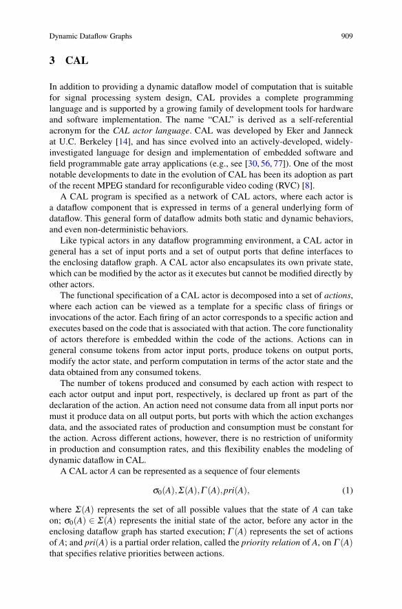
Fig. 3 An illustration of the design of a switch actor in CFDF
Figures 3 and 4 illustrate, respectively, the design of a CFDF actor and its imple-mentation in functional DIF. This actor provides functionality that is equivalent tothe Boolean dataflow switch actor described in Sect. 2.
6 Scenario Aware Dataflow
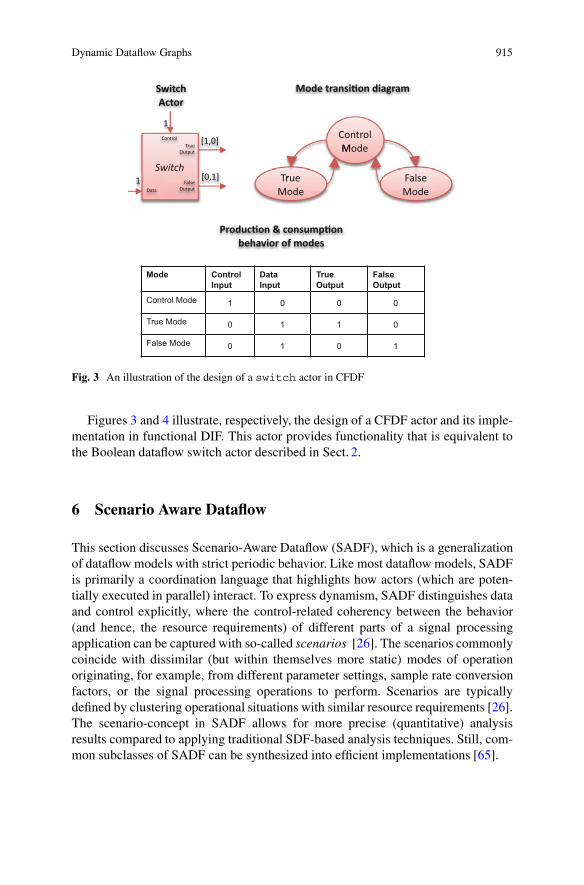
This section discusses Scenario-Aware Dataflow (SADF), which is a generalizationof dataflow models with strict periodic behavior. Like most dataflow models, SADFis primarily a coordination language that highlights how actors (which are poten-tially executed in parallel) interact. To express dynamism, SADF distinguishes dataand control explicitly, where the control-related coherency between the behavior(and hence, the resource requirements) of different parts of a signal processingapplication can be captured with so-called scenarios [26]. The scenarios commonlycoincide with dissimilar (but within themselves more static) modes of operationoriginating, for example, from different parameter settings, sample rate conversionfactors, or the signal processing operations to perform. Scenarios are typicallydefined by clustering operational situations with similar resource requirements [26].The scenario-concept in SADF allows for more precise (quantitative) analysisresults compared to applying traditional SDF-based analysis techniques. Still, com-mon subclasses of SADF can be synthesized into efficient implementations [65].

916 S.S. Bhattacharyya et al.
Fig. 4 An implementation of the switch actor design of Fig. 3 in the functional DIF environment
6.1 SADF Graphs
In this subsection SADF is introduced by some examples from the multi-mediadomain. Consider the MPEG-4 video decoder for the Simple Profile from [66, 70].It supports video streams consisting of intra (I) and predicted (P) frames. For animage size of 176× 144 pixels (QCIF), there are 99 macro blocks to decode forI frames and no motion vectors. For P frames, such motion vectors determine thenew position of certain macro blocks relative to the previous frame. The numberof motion vectors and macro blocks to process for P frames ranges between 0 and99. The MPEG-4 decoder clearly shows variations in the functionality to performand in the amount of data to communicate between the operations. This leads tolarge fluctuations in resource requirements [52]. The order in which the differentsituations occur strongly depends on the video content and is generally not periodic.
Figure 5 depicts an SADF graph for the MPEG-4 decoder in which nine differentscenarios are identified. SADF distinguishes two types of actors: kernels (solidvertices) model the data processing parts, whereas detectors (dashed vertices)

Dynamic Dataflow Graphs 917
d
a
11
1
1
d
1
1
1
1
b
1
c
1
1
d
e
31
1
c
IDCTVLD
MCRCFD
Actor (Sub)Scenario E (kCycles)
VLDP0 0
All except P0 40
IDCTP0 0
All except P0 17
MC
I, P0 0P30 90P40 145P50 190P60 235P70 265P80 310P99 390
RC
I 350P0 0
P30 , P40 , P50 250P60 300
P70 , P80 , P99 320
FD All 0
Rate(Sub)ScenarioI P0 Px
a 0 0 1b 0 0 x
c 99 1 x
d 1 0 1e 99 0 x
x ∈ { 30 , 40 , 50 , 60 , 70 , 80 , 99}
a
b
c
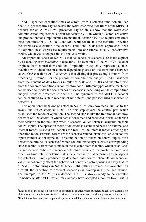
Fig. 5 Modeling the MPEG-4 decoder with SADF. (a) Actors and channels; (b) parameterizedrates; (c) worst-case execution times
control the behavior of actors through scenarios.2 Moreover, data channels (solidedges) and control channels (dashed edges) are distinguished. Control channelscommunicate scenario-valued tokens that influence the control flow. Data tokens donot influence the control flow. The availability of tokens in channels is shown witha dot. Here, such dots are labeled with the number of tokens in the channel. Thestart and end points of channels are labeled with production and consumption ratesrespectively. They refer to the number of tokens atomically produced respectivelyconsumed by the connected actor upon its firing. The rates can be fixed or scenario-dependent, similar as in PSDF. Fixed rates are positive integers. Parameterizedrates are valued with non-negative integers that depend on the scenario. Theparameterized rates for the MPEG-4 decoder are listed in Fig. 5b. A value of0 expresses that data dependencies are absent or that certain operations are notperformed in those scenarios. Studying Fig. 5b reveals that for any given scenario,the rate values yield a consistent SDF graph. In each of these scenario graphs,detector FD has a repetition vector entry of 1 [70], which means that scenariochanges as prescribed by the behavior of detectors may occur only at iterationboundaries of each such scenario graph. This is not necessarily true for SADF ingeneral as discussed below.
2In case of one detector, SADF literature may not show the detector and control channels explicitly.
918 S.S. Bhattacharyya et al.
SADF specifies execution times of actors (from a selected time domain, seeSect. 6.2) per scenario. Figure 5c lists the worst-case execution times of the MPEG-4decoder for an ARM7TDMI processor. Figure 5b, c show that the worst-casecommunication requirements occur for scenario P99, in which all actors are activeand production/consumption rates are maximal. Scenario P99 also requires maximalexecution times for VLD, IDCT, and MC, while for RC it is the scenario I in whichthe worst-case execution time occurs. Traditional SDF-based approaches needto combine these worst-case requirements into one (unrealistically) conservativemodel, which yields too pessimistic analysis results.
An important aspect of SADF is that sequences of scenarios are made explicitby associating state machines to detectors. The dynamics of the MPEG-4 decoderoriginate from control-flow code that (implicitly or explicitly) represents a state-machine with video stream content dependent guards on the transitions betweenstates. One can think of if-statements that distinguish processing I frames fromprocessing P frames. For the purpose of compile-time analysis, SADF abstractsfrom the content of data tokens (similar to SDF and CSDF) and therefore alsofrom the concrete conditions in control-flow code. Different types of state machinescan be used to model the occurrences of scenarios, depending on the compile-timeanalysis needs as presented in Sect. 6.2. The dynamics of the MPEG-4 decodercan be captured by a state-machine of nine states (one per scenario) associated todetector FD.
The operational behavior of actors in SADF follows two steps, similar to theswitch and select actors in BDF. The first step covers the control part whichestablishes the mode of operation. The second step is like the traditional data flowbehavior of SDF actors3 in which data is consumed and produced. Kernels establishtheir scenario in the first step when a scenario-valued token is available on theircontrol inputs. The operation mode of detectors is established based on external andinternal forces. Subscenario denotes the result of the internal forces affecting theoperation mode. External forces are the scenario-valued tokens available on controlinputs (similar as for kernels). The combination of tokens on control inputs for adetector determine its scenario,4 which (deterministically) selects a correspondingstate-machine. A transition is made in the selected state machine, which establishesthe subscenario. Where the scenario determines values for parameterized rates andexecution time details for kernels, it is the subscenario that determines these aspectsfor detectors. Tokens produced by detectors onto control channels are scenario-valued to coherently affect the behavior of controlled actors, which is a key featureof SADF. Actor firings in SADF block until sufficient tokens are available. Asa result, the execution of different scenarios can overlap in a pipelined fashion.For example, in the MPEG-4 decoder, IDCT is always ready to be executedimmediately after VLD, which may already have accepted a control token with a
3Execution of the reflected function or program is enabled when sufficient tokens are available onall (data) inputs, and finalizes (after a certain execution time) with producing tokens on the outputs.4If a detector has no control inputs, it operates in a default scenario ε and has one state machine.
Dynamic Dataflow Graphs 919
RQL ROL ARL IMDCTL FIL SPFL576
576
bb
b
f
fi
ii
l
l
l
576576
1152RQR ROR
S
ARR IMDCTR FIR SPFRd
d
d hj
j j n
n
n
576 576
11521152
1152 WH
g
e
k
m
g
c
h
a
e
FD BDR
2
1
1
1
1
1
x1
1
1
1
BDL
1
y y
1
zz
1
1
11
1
x
1
1 1
9
1
z
y
1
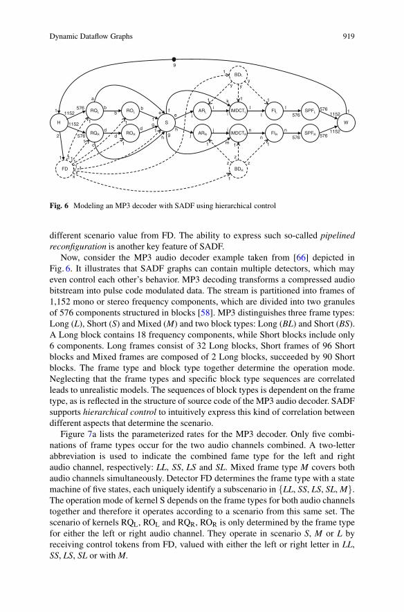
Fig. 6 Modeling an MP3 decoder with SADF using hierarchical control
different scenario value from FD. The ability to express such so-called pipelinedreconfiguration is another key feature of SADF.
Now, consider the MP3 audio decoder example taken from [66] depicted inFig. 6. It illustrates that SADF graphs can contain multiple detectors, which mayeven control each other’s behavior. MP3 decoding transforms a compressed audiobitstream into pulse code modulated data. The stream is partitioned into frames of1,152 mono or stereo frequency components, which are divided into two granulesof 576 components structured in blocks [58]. MP3 distinguishes three frame types:Long (L), Short (S) and Mixed (M) and two block types: Long (BL) and Short (BS).A Long block contains 18 frequency components, while Short blocks include only6 components. Long frames consist of 32 Long blocks, Short frames of 96 Shortblocks and Mixed frames are composed of 2 Long blocks, succeeded by 90 Shortblocks. The frame type and block type together determine the operation mode.Neglecting that the frame types and specific block type sequences are correlatedleads to unrealistic models. The sequences of block types is dependent on the frametype, as is reflected in the structure of source code of the MP3 audio decoder. SADFsupports hierarchical control to intuitively express this kind of correlation betweendifferent aspects that determine the scenario.
Figure 7a lists the parameterized rates for the MP3 decoder. Only five combi-nations of frame types occur for the two audio channels combined. A two-letterabbreviation is used to indicate the combined fame type for the left and rightaudio channel, respectively: LL, SS, LS and SL. Mixed frame type M covers bothaudio channels simultaneously. Detector FD determines the frame type with a statemachine of five states, each uniquely identify a subscenario in {LL, SS, LS, SL, M}.The operation mode of kernel S depends on the frame types for both audio channelstogether and therefore it operates according to a scenario from this same set. Thescenario of kernels RQL, ROL and RQR, ROR is only determined by the frame typefor either the left or right audio channel. They operate in scenario S, M or L byreceiving control tokens from FD, valued with either the left or right letter in LL,SS, LS, SL or with M.

920 S.S. Bhattacharyya et al.
RateScenario
L S Ma, c 576 0 36b, d 0 576 540
Rate(Sub)Scenario
LL SS LS SL Me 0 576 0 576 36f 576 0 576 0 540g 0 576 576 0 540h 576 0 0 576 36x 1 1 1 1 2
RateScenarioBL BS
i, j 18 0k, m 0 6l, n 18 6
RateSubScenario
LBL SBS MBL MBSy, z 32 96 2 90
ScenarioL ScenarioS
LBL SBS
ScenarioM
MBS MBL
a b
Fig. 7 Properties of the MP3 decoder model. (a) Parameterized rates; (b) state machines for BDLand BDR
Detectors BDL and BDR identify the appropriate number and order of Short andLong blocks based on the frame scenario, which they receive from FD as controltokens valued L, S or M. From the perspective of BDL and BDR, block types BLand BS are refinements (subscenarios) of the scenarios L, S and M. Figure 7b showsthe three state machines associated with BDL as well as BDR. Each of their statesimplies one of the possible subscenarios in {LBL,SBS,MBL,MBS}. The valueof the control tokens produced by BDL and BDR to kernels ARL, IMDCTL, FIL
and ARR, IMDCTR, FIR in each of the four possible subscenarios matches the lasttwo letters of the subscenario name (i.e., BL or BS). Although subscenarios LBLand MBL both send control tokens valued BL, the difference between them is thenumber of such tokens (similarly for subscenarios SBS and MBS).
Consider decoding of a Mixed frame. It implies the production of two M-valuedtokens on the control port of detector BDL. By interpreting each of these tokens,the state machine for scenario M in Fig. 7b makes one transition. Hence, BDL usessubscenario MBL for its first firing and subscenario MBS for its second firing. Insubscenario MBL, BDL sends 2 BL-valued tokens to kernels ARL, IMDCTL andSPFL, while 90 BS-valued tokens are produced in subscenario MBS. As a result,ARL, IMDCTL and SPFL first process 2 Long blocks and subsequently 90 Shortblocks as required for Mixed frames.
The example of Mixed frames highlights a unique feature of SADF: reconfigu-rations may occur during an iteration. An iteration of the MP3 decoder correspondsto processing frames, while block type dependent variations occur during process-ing Mixed frames. Supporting reconfiguration within iterations is fundamentallydifferent from assumptions underlying other dynamic dataflow models, includingfor example PSDF. The concept is orthogonal to hierarchical control. Hierarchicalcontrol is also different from other dataflow models with hierarchy such asheterochronous dataflow [27]. SADF allows pipelined execution of the controllingand controlled behavior together, while other approaches commonly prescribe thatthe controlled behavior must first finish completely before the controlling behaviormay continue.

Dynamic Dataflow Graphs 921
6.2 Analysis
Various analysis techniques exist for SADF, allowing the evaluation of both quali-tative properties (such as consistency and absence of deadlock) and best/worst-caseand average-case quantitative properties (like minimal and average throughput).
Consistency of SADF graphs is briefly discussed now. The MPEG-4 decoder isan example of a class of SADF graphs where each scenario is like a consistent SDFgraph and scenario changes occur at iteration boundaries of these scenario graphs(but still pipelined). Such SADF graphs are said to be strongly consistent [70], whichis easy to check as it results from structural properties only. The SADF graph of theMP3 decoder does not satisfy these structural properties (for Mixed frames), but itcan still be implemented in bounded memory. The required consistency propertyis called weak consistency [66]. Checking weak consistency requires taking thepossible (sub)scenario sequences as captured by the state machines associated todetectors into account, which complicates a consistency check considerably.
Analysis of quantitative properties and the efficiency of the underlying tech-niques depend on the selected type of state machine associated to detectors as wellas the chosen time model. For example, one possibility is to use non-deterministicstate machines, which merely specify what sequences of (sub)scenarios can occurbut not how often. This is typically used for best/worst-case analysis. Applying thetechniques in [20, 23, 24] then allows computing that a throughput of processing0.253 frames per kCycle can be guaranteed for the MPEG-4 decoder. An alternativeis to use probabilistic state machines (i.e., Markov chains), which additionallycapture the occurrence probabilities of the (sub)scenario sequences to allow foraverage-case analysis as well. Assuming that scenarios I, P0, P30, P40, P50, P60, P70,P80 and P99 of the MPEG-4 decoder may occur in any order and with probabilities0.12, 0.02, 0.05, 0.25, 0.25, 0.09, 0.09, 0.09 and 0.04 respectively, the techniquesin [67] allow computing that the MPEG-4 decoder processes on average 0.426frames per kCycle. The techniques presented in [71] combine the associationof Markov chains to detectors with exponentially distributed execution times toanalyze the response time distribution of the MPEG-4 decoder for completing thefirst frame.
The semantics of SADF graphs where Markov chains are associated to detectorswhile assuming generic discrete execution time distributions5 has been definedin [66] using Timed Probabilistic Systems (TPS). Such transition systems opera-tionalize the behavior with states and guarded transitions that capture events likethe begin and end of each of the two steps in firing actors and progress of time.In case an SADF graph yields a TPS with finite state space, it is amenable toanalysis techniques for (Priced) Timed Automata or Markov Decision Processes andMarkov Chains by defining reward structures as also used in (probabilistic) modelchecking. Theelen et al. [67] discusses that specific properties of dataflow models in
5This covers the case of constant execution times as so-called point distributions [66, 67].

922 S.S. Bhattacharyya et al.
general and SADF in particular allow for substantial state-space reductions duringsuch analysis. The underlying techniques have been implemented in the SDF3 toolkit [62], covering the computation of worst/best-case and average-case propertiesfor SADF including throughput and various forms of latency and buffer occupancymetrics [68]. In case such exact computation is hampered by state-space explosion,[68,70] exploit an automated translation into process algebraic models expressed inthe Parallel Object-Oriented Specification Language (POOSL) [69], which allowsfor statistical model checking (simulation-based estimation) of the properties. Thecombination of Markov chains and exponentially distributed execution times hasbeen studied in [71], using a process algebraic semantics based on InteractiveMarkov Chains [33] to apply a general-purpose model checker for analyzingresponse time distributions.
In case we abstract from the stochastic aspects of execution times and scenariooccurrences, SADF is still amenable to worst/best-case analysis. Since SADFgraphs are timed dataflow graphs, they exhibit linear timing behavior [20, 43, 76],which facilitates network-level worst/best-case analysis by considering the worst/best-case execution times for individual actors. For linear timed systems this isknow to lead to the overall worst/best-case performance. For the class of strongly-consistent SADF graphs with a single detector (also called FSM-based SADF ),very efficient performance analysis can be done based on a (max,+)-algebraicinterpretation of the operational semantics. It allows for worst-case throughputanalysis, some latency analysis and can find critical scenario sequences withoutexploring the state-space of the underlying TPS. Instead, the analysis is performedby means of state-space analysis and maximum-cycle ratio analysis of the equivalent(max,+)-automaton [20, 23, 24]. Geilen et al. [23] shows how this analysis canbe extended for the case that scenario behaviors are not complete iterations of thescenario SDF graphs.
6.3 Synthesis
FSM-based SADF graphs have been extensively studied for implementation on(heterogeneous) multi-processor platforms [64]. Variations in resource requirementsneed to be exploited to limit resource usage without violating any timing require-ments. The result of the design flow for FSM-based SADF implemented in the SDF3
tool kit [62] is a set of Pareto optimal mappings that provide a trade-off in validresource usages. For certain mappings, the application may use many computationalresources and few storage resources, whereas an opposite situation may exist forother mappings. At run-time, the most suitable mapping is selected based on theavailable resources not used by concurrently running applications [59].
There are two key aspects of the design flow of [62, 64]. The first concernsmapping channels onto (possibly shared) storage resources. Like other dataflowmodels, SADF associates unbounded buffers with channels, but a complete graphmay still be implemented in bounded memory. FSM-based SADF allows for

Dynamic Dataflow Graphs 923
Fig. 8 Throughput/buffer size trade-off space for the MPEG-4 decoder
efficient compile-time analysis of the impact that certain buffer sizes have on thetiming of the application. Hence, a synthesized implementation does not requirerun-time buffer management, thereby making it easier to guarantee timing. Thedesign flow in [64] dimensions the buffer sizes of all individual channels in the graphsufficiently large to ensure that timing (i.e., throughput) constraints are met but alsoas small as possible to save memory and energy. It exploits the techniques of [63]to analyze the trade-off between buffer sizes and throughput for each individualscenario in the FSM-based SADF graph. After computing the trade-off space forall individual scenarios, a unified trade-off space for all scenarios is created. Thesame buffer size is assigned to a channel in all scenarios. Combining the individualspaces is done using Pareto algebra [22] by taking the free product of all trade-offspaces and selecting only the Pareto optimal points in the resulting space. Figure 8shows the trade-off space for the individual scenarios in the MPEG-4 decoder.In this application, the set of Pareto points that describe the trade-off betweenthroughput and buffer size in scenario P99 dominate the trade-off points of all otherscenarios. Unifying the trade-off spaces of the individual scenarios therefore resultsin the trade-off space corresponding to scenario P99. After computing the unifiedthroughput/buffer trade-off space, the synthesis process in [64] selects a Pareto pointwith the smallest buffer size assignment that satisfies the throughput constraint as ameans to allocate the required memory resources in the multiprocessor platform.

924 S.S. Bhattacharyya et al.
A second key aspect of the synthesis process is the fact that actors of thesame or different applications may share resources. The set of concurrently activeapplications is typically unknown at compile-time. It is therefore not possible toconstruct a single static-order schedule for actors of different applications. Thedesign flow in [64] uses static-order schedules for actors of the same application,but sharing of resources between different applications is handled by run-timeschedulers with TDMA policies. It uses a binary search algorithm to compute theminimal TDMA time slices ensuring that the throughput constraint of an applicationis met. By minimizing the TDMA time slices, resources are saved for otherapplications. Identification of the minimal TDMA time slices works as follows.In [3], it is shown that the timing impact of a TDMA scheduler can be modeledinto the execution time of actors. This approach is used to model the TDMA timeslice allocation it computes. Throughput analysis is then performed on the modifiedFSM-based SADF graph. When the throughput constraint is met, the TDMA timeslice allocation can be decreased. Otherwise it needs to be increased. This processcontinues until the minimal TDMA time slice allocation satisfying the throughputconstraint is found.
7 Dynamic Polyhedral Process Networks
The chapter on polyhedral process networks (PPN) [73] deals with the auto-matic derivation of certain dataflow networks from static affine nested loop pro-grams (SANLP). An SANLP is a nested loop program in which loop bounds,conditions and variable index expressions are (quasi-)affine expressions in theiterators of enclosing loops and static parameters.6 Because many signal processingapplications are not static, there is a need to consider dynamic affine nested loopprograms (DANLP) which differ from SANLPs in that they can contain
1. If-the-else constructs with no restrictions on the condition [60].2. Loops with no condition on the bounds [44].3. While statements other than while(1) [45].4. Dynamic parameters [78].
Remark. In all DANLP programs presented in subsequent subsections, arrays areindexed by affine functions of static parameters and enclosing for-loop iterators.This is why the A is still in the name.
6The corresponding tool is called PNgen [74], and is part of the Daedalus design frame-work [48], http://daedalus.liacs.nl.

Dynamic Dataflow Graphs 925
1 %parameter N 8 16;23 for i = 1:1:N,4 [x(i), t(i)] = F1(...);5 end6
7 for i = 1:1:N,8 if t(i) <= 0,9 [x(i)] = F2( x(i) );10 end11 [...] = F3( x(i) );12 end
Fig. 9 Pseudo code of a simple weakly dynamic program
1 %parameter N 8 16;23 for i = 1:1:N,4 ctrl(i) = N+1;5 end6 for i = 1:1:N,7 [out_0, out_1] = F1(...);8 [x_1(i)] = opd(out_0);9 [t_1(i)] = opd(out_1);10 end1112 for i = 1:1:N,13 [t_1(i)] = ipd(t_1(i));14 if t_1(i) <= 0,15 [in_0] = ipd(x_1(i));
16 [out_0] = F2(in_0);17 [x_2(i)] = opd(out_0);18 [ ctrl(i) ] = opd( i );19 end2021 C = ipd( ctrl(i) );22 if i = C,23 [in_0] = ipd(x_2(C));24 else25 [in_0] = ipd(x_1(i));26 end2728 [out_0] = F3(in_0);29 [...] = opd(out_0);30 end
Fig. 10 Example of dynamic single assignment code
7.1 Weakly Dynamic Programs
While in a SANLP condition statements must be affine in static parameters anditerators of enclosing loops, if conditions can be anything in a DANLP. Suchprograms have been called weakly dynamic programs (WDP) in [60]. A simpleexample of a WDP is shown in Fig. 12.
The question of course is whether the argument of function F3 originates fromthe output of function F2 or function F1.
In the case of a SANLP, the input–output equivalent PPN is obtained by(1) converting the SANLP—by means of an array analysis [16, 17]—to a singleassignment code (SAC) used in the compiler community and the systolic arraycommunity (see [34]); (2) deriving from the SAC a polyhedral reduced dependencegraph [55] (PRDG); and (3) constructing the PPN from the PRDG [13, 39, 55].
While in a SAC every variable is written only once, in a dynamic singleassignment code (dSAC) every variable is written at most once. For some variables,it is not known whether or not they will be read or written at compile time. For aWDP, however, not all dependences are known at compile time and, therefore, theanalysis must be based on the so-called fuzzy array dataflow analysis [18]. Thisapproach allows the conversion of a WDP to a dSAC. The procedure to generate thedSAC is out of the scope of this chapter. The dSAC for the WDP in Fig. 9 is shownin Fig. 10.
926 S.S. Bhattacharyya et al.
C in the dSAC shown in Fig. 10 is a parameter emerging from the if-statement inline 8 of the original program shown in Fig. 9. This if-statement also appears in thedSAC in line 14. The dynamic change of the value of C is accomplished by the lines18 and 21 in Fig. 10. The control variable ctrl(i) in line 18 stores the iterationsfor which the data dependent condition that introduces C is true. Also, the variablectrl(i) is used in line 21 to assign the correct value to C for the current iteration.See [60] for more details.
The dSAC can now be converted to two graph structures, namely the Approxi-mate reduced dependence graph (ADG), and the Schedule tree (STree). The ADGis the dynamic counterpart of the static PRDG. Both the PRDG and the ADG arecomposed of processes N, input ports IP, output ports OP, and edges E [13, 55].They contain all information related to the data dependencies between functions inthe SAC and the dSAC, respectively. However, in a WDP some dependencies arenot known at compile time, hence the name approximate. Because of this, the ADGhas the additional notion of linearly bounded set, as follows.
Let be given four sets of functionsS1 = { f 1
x (i) | x = 1..|S1|, i ∈ Zn}, S2 = { f 2x (i) | x = 1..|S2|, i ∈ Zn}, S3 =
{ f 3x (i) | x = 1..|S3|, i ∈ Zn}, S4= { f 4
x (i) | x = 1..|S4|, i ∈ Zn}, an integral m × nmatrix A and an integral n-vector b. A linearly bounded set (LBS) is a set of pointsLBS = { i ∈ Zn | A.i ≥ b,
i f S1 �≡ /0 ⇒ ∀ x=1..|S1|, f 1x (i)≥ 0,
i f S2 �≡ /0 ⇒ ∀ x=1..|S2|, f 2x (i)≤ 0,
i f S3 �≡ /0 ⇒ ∀ x=1..|S3|, f 3x (i)> 0,
i f S4 �≡ /0 ⇒ ∀ x=1..|S4|, f 4x (i)< 0 }.
The set of points B = { i ∈ Zn | A.i ≥ b } is called linear bound of the LBS andthe set S = S1 ∪ S2 ∪ S3 ∪ S4 is called filtering set. Every f j
x (i) ∈ S can be anarbitrary function of i.
Consider the dSAC shown in Fig. 10. The exact iterations i are not known atcompile time because of the dynamic condition at line 14 in the dSAC (Fig. 10).That is why the notion of linearly bounded set is introduced, by which the unknowniterations i are approximated. So, NDN2 is the following LBS: NDN2 = {i ∈ Z | 1 ≤i ≤ N ∧ 8 ≤ N ≤ 16, t 1(i) ≤ 0}. The linear bound of this LBS is the polytopeB = {1 ≤ i ≤ N∧8 ≤ N ≤ 16} that captures the information known at compile timeabout the bounds of the iterations i. The variable t 1(i) is interpreted as an unknownfunction of i called filtering function whose output is determined at run time.
The STree contains all information about the execution order amongst thefunctions in the dSAC. The STree represents one valid schedule between all thesefunctions called global schedule. From the STree a local schedule between anyarbitrary set of the functions in the dSAC can be obtained by pruning operationson the STree. Such a local schedule may for example be needed when two or moreprocesses are merged [61]. The STres is obtained by converting the dSAC to a syntaxtree using a standard syntax parser, after which all the nodes and edges that are notrelated to nodes Fi (nodes F1, F2, and F3 in Fig. 10). See [60] for further details.A summary is depicted in Fig. 11.

Dynamic Dataflow Graphs 927
N1(F1)
q2
q1
p1
q1
q2
p1
p2
p2p2
(F2)
N3(F3)
q2
p1
q1
q2
p1
p2
p2
N2(F2)
N3(F3)
q11N1(F1)
p3q12
N2ED5(ctrl)
ED4(x_2)
ED2(
x_1)
ED3(x_1)
a
b
c
d
ED5(ctrl)
ED3(x_1)
ED2(
x_1)
ED4(x_2)
STree Marking
OG2
OG2
OG1
IG1
IG1 OG1
IG3
IG2(N2)P1
C1( ED5 )
C2( ED4 )
C3( ED1&ED2 )
C4( ED3 )P2
F1 F2
STree Pruning
F1 F2
F1
root
root
rootfor i = 1:1:Nfor i = 1:1:N
for i = 1:1:Nfor i = 1:1:N
for i = 1:1:N for i = 1:1:NED1(t_1)
ED1(t_1)
F3
F3
F3
(N1&N3)
if t_1(i) <= 0
if t_1(i) <= 0
Fig. 11 Examples of (a) approximated dependence graph (ADG) model; (b) transformed ADG;(c) schedule tree and transformations; (d) process network model
The difference between the ADG in Fig. 11a and the transformed ADG inFig. 11b is that an ADG may have several input ports connected to a single outputport whilst in the transformed ADG every input port is connected to only one singleoutput port (in accordance with the Kahn Process Network semantics [35]).
Parsing the STree in Fig. 11c top-down from left to right generates a programthat gives a valid execution order (global schedule) among the functions F1, F2 andF3 which is the original order given by the dSAC.
The process network in Fig. 11d may be the result of a design space exploration,and some optimizations. For example, process P2 is constructed by grouping nodesN1 and N3 in the ADG in Fig. 11b. Because the behavior of process P2 is sequential(by default), it has to execute the functionality of nodes N1 and N3 in sequentialorder. This order is obtained from the STree in Fig. 11c. See [60] for details.

928 S.S. Bhattacharyya et al.
1 %parameter N 1 10;23 for j = 1 to N,4 for i = 1 to f(...),5 y[ i ] = F1()6 end7 end8 [...] = F2( y[5] ),
An example of a Dynloop program.
1 %parameter N 1 10;23 for j = 1 to N,4 X[j] = f(...)5 for i = 1 to max f,6 if i <= X[j] ,7 y[i] = F1()8 end9 end10 end11 [] = F2( y[5] )
An equivalent WeaklyDynamic Program.
Fig. 12 A Dynloop program and its equivalent WDP program
In a (static) PPN, there are two models of FIFO communication [72], namelyin-order communication and out-of-order communication. In the first model, theorder in which tokens are read from a FIFO channel is the same as the order inwhich they have been written to the channel. In the second model that order isdifferent. In a PPN that is input–output equivalent to a WDP, there are two moreFIFO communication models, namely in-order with coloring and out-of-order withcoloring. This is necessary because the number of tokens that will be written toa channel and read from that channel is not known at compile time. See [60] fordetails.
Buffer sizes can be determined using the procedure given in [73] and in [74],except that a conservative strategy (over-estimation) is needed due to the fact that therate and the exact amount of data tokens that will be transferred over a particular datachannel is unknown at compile-time. This can be done by modifying the iterationdomains of all input/output ports, such that all dynamic if-conditions defining anyof these iteration domains evaluate always to true.
7.2 Dynamic Loop-Bounds
Whereas in a SANLP loop bounds have to be affine functions of iterators ofenclosing loops and static parameters, loop bounds in a DANLP program can bedynamic. Such programs have been called Dynloop programs in [44]. A simpleexample of a Dynloop program is shown at the left side in Fig. 12
A Dynloop program can be cast in the form of a WDP. See Sect. 7.1. The WDPcorresponding to the Dynloop program at the left in Fig. 12 is shown at the rightin Fig. 12.

Dynamic Dataflow Graphs 929
1 %parameter N 1 10;
2 for j = 1 to N,3 X[j] = f()4 for i = 1 to max_f,5 if i <= X[j],6 y_1[j,i] = F1()7 ctrl_c1[i] = j8 ctrl_c2[i] = i9 end10 ctrl c1 1[j,i] = ctrl c1[i]11 ctrl c2 1[j,i] = ctrl c2[i]12 end13 end
14 if max f >= 5,15 c1 = ctrl c1 1[N, 5]16 c2 = ctrl c2 1[N, 5]17 else18 c1 = N + 119 c2 = max f + 120 end21 if c1 <= N & c2 == 5,22 in_0 = y_1[c1,c2]23 else24 in_0 = 025 end26 [...] = F2( in_0 )
Fig. 13 Final dSAC
The maximum value of f (), denoted by max f, see line 5 at the right in Fig. 12is substituted for the upper bound of the loop at line 4 at the left in Fig. 12. Thevalue of max f can be determined by studying the range of function f ().7
As in Sect. 7.1, a dynamic single assignment code (dSAC) can now be obtainedby means of a fuzzy array dataflow analysis (FADA) [18]. This analysis introducesparameters to deal with the dynamic structure in the WDP. The values of theseparameters have to be changed dynamically. This is done by introducing for everysuch parameter a control variable that stores the correct value of the parameter forevery iteration. However, the straightforward introduction of control values as donein Sect. 7.1 violates the dSAC condition that every control variable is written atmost once. To obtain a valid dSAC, an additional dataflow analysis for the controlvariables is necessary, resulting in additional control variables. See [44] for details.
The final dSAC is shown in Fig. 13 where it has been assumed that the variabley(5) has been initialized to zero.
The control variables must be initialized with values that are greater thanthe maximum value of the corresponding parameters. For the example at hand,parameter c1 ∈ [1..N], and c2 ∈ [1..max f]. Therefore, the corresponding controlvariables are initialized as follows:
∀i : 1 ≤ i≤ max f : ctrl c1[i]= N+ 1,ctrl c2[i]= max f+ 1.
This initialization is not shown in Fig. 13 for the sake of brevity.After applying the standard linearization [72], and its extension described in
Sect. 7.1, and estimating buffer sizes as described in that same subsection, theresulting PPN is as shown in Fig. 14.
7If that is not possible, then an alternative way to estimate max f is given in [44].

930 S.S. Bhattacharyya et al.
1 for j = 1 to N,2 read(i1, in_1)3 for i = 1 to max_f,4 if i <= in_1,5 y_1[j,i] = F1()6 ctrl_c1[i] = j7 ctrl_c2[i] = i8 endif9 if j=N and i=510 out_1 = ctrl_c1[i] 11 out_2 = ctrl_c2[i] 12 out_3 = y_1[ctrl_c1[i], ctrl_c2[i]]13 write(o1, out_1)14 write(o2, out_2)15 write(o3, out_3)16 endif17 endfor18 endfor
Process P2
i1
i3
i2
1 if max_f >= 5,2 read(i1, in_1)3 read(i2, in_2)4 read(i3, in_3)5 else6 in_1 = N+1
9 if in_1 <= N & in_2 == 5,
11 else12 in_4 = 013 endif14 [] = F2( in_4 )
8 endif7 in_2 = max_f+1
10 in_4 = in_3
Process P3Process P1
o1
1 for j = 1 to N,2 out_1 = f();3 write(o1, out_1);4 endfor
i1
o3
o2o1
Fig. 14 The final PPN derived from the program in Fig. 13
7.3 Dynamic While-Loops
Whereas in a SANLP program only while(1)loops are allowed, in a DANLPprogram any while-loop is acceptable. Such DANLP programs have been calledwhile-loop affine programs (WLAP) in [45].
There are a number of publications that address the problem of while loopsparallelization [4, 10, 12, 25, 28, 29, 53, 54]. The approach presented here has theadvantage that it
• Supports both task-level and data-level parallelism.• Generates also parallel code for multi-processor systems having distributed
memory.• Provides an automatic data-dependence analysis procedure.• Exposes and utilizes all available parallelism.
An example is shown at the left side in Fig. 15.Again, the question is from where, say, function F7 gets its scalar argument
x. Because this is not known at compile-time, a fuzzy array dataflow analysis(FADA) [18] is necessary to find all data dependencies.
The approach to convert a WLAP program to an input–output equivalentpolyhedral process network (PPN) goes in four steps. First, all data-dependencyrelations in the initial WLAP program have to be found by applying the FADAanalysis on it. Recall that the result of the analysis is approximated, i.e., it dependson parameters which values are determined at run-time. Second, based on the resultsof the analysis, the initial WLAP is transformed into a dynamic Single AssignmentCode (dSAC) representation. See Sect. 7.1. Parameters that are introduced by theFADA appear in the dSAC, and their values are assigned using control variables.Third, the control variables are generated in a way that extends the methods inSects. 7.1 and 7.2 to be applicable for WLAP programs as well, see [45]. Fourth,the topology of the corresponding PPN is derived as well as the code to be executedin the processes of the PPN.

Dynamic Dataflow Graphs 931
1 ¶meter EPS 0.005
2 for i = 1 to N,3 y[i] = F1()4 x = F2( y[i] )5 while ( x >= EPS )6 x = F3()7 for j = i+1 to N+1,8 y[j] = F4( y[j-1] )9 x = F5( x, y[j] )10 end11 y[i] = F6( x )12 end13 out = F7( x )14 end
1 %parameter EPS 0.005
2 w = 03 ctrl_x_5 = (N+1,0)4 for i = 1 to N,5 y_1[i] = F1()6 in_2 = y_1[i]7 x_2[i] = F2( in_2 )8 while (in_w = σx( W,(i,w) ) >= EPS),9 w = w + 111 x_3[i,w] = F3()11 for j = i+1 to N+1,12 in_4 = σy( S4,(i,w, j) )13 y_4[i,w,j] = F4( in_4 )14 in_5_x = σx( S5,(i,w, j) )15 in_5_y = y_4[i,w,j]16 x_5[i,w,j] = F5( in_5_x, in_5_y )17 ctrl x 5 = (i,w)18 end19 in_6 = σx( S6,(i,w) )20 y_6[i,w] = F6( in_6 )21 end22 ctrl x 5 [i] = ctrl x 523 (a ,b
a b) = ctrl x 5 [i]
24 in_7 = σx( S7,(i, , ) )25 out = F7( in_7 )26 end
An example of a WLAP program The corresponding final dSAC
Fig. 15 An example of a while-loop affine program and its corresponding dynamic singleassignment program
The iterator w is associated with the while loop and is initialized with value 0,meaning that the while loop has never been executed. The parameter α capturesthe value of the for-loop iterator in the enclosing while-loop and is initialized toN + 1. The parameter β is the upper bound of the while-loop iterator w. Becauseα ∈ [1..N] and β ≥ 1, the above initializations satisfy the condition that their valuesare never taken by the corresponding parameters. From line 23 at the right sidein Fig. 15, it follows that the control variable ctrl x 5 is initialized to ctrl x 5= (N+1,0) at line 3 at the right side in Fig. 15. Where does the control variablectrl x 5 come from? It comes from the construction of the dSAC. The procedureto derive the final dSAC is largely based on [18] and its extension in Sect. 7.2.The problem is again that the dSAC resulting from the FADA analysis is not aproper dSAC because it violates the property that every variable is written at mostonce. The relation between writing to and reading from the control variables mustbe identified by performing a dataflow analysis for the control variables, wherethe writings to them occur inside a while-loop. To that end, an additional controlvariable ctrl x 5 is introduced right after the while-loop, see line 22 at the rightin Fig. 15. The new control variable is written at every iteration of for-loop i andtakes the value either of control variable ctrl x 5 assigned on the last iteration ofthe while-loop, or its initial value, if the while-loop is not executed. A static exact

932 S.S. Bhattacharyya et al.
P1
P2y_1[]
P4
y_4[]
W
x_2[] P7
x_2[]
P3P5
P6
ctrl_x_5_[]
y_6[]
Fig. 16 The PPN for the program in Fig. 15
1 %parameter EPS 0.005
2 w = 03 for i = 1 to N,4 while(1),5 w = w + 16 if (w > 2) then w = 27 if (w == 1),8 read(P2, 1, in w)9 else10 read(P5, 2, in w)11 end12 out_w = (in_w >= EPS)13 write(P3, 3, out w)14 write(P4, 4, out w)15 write(P5, 5, out w)16 write(P6, 6, out w)17 if (!out_w) <break>18 end19 end
Code of process W
1 w = 02 ctrl_x_5 = (N+1,0)3 for i = 1 to N,4 while(1),5 w = w + 16 if (w > 2) then w = 27 read(W, 1, in w)8 if (!in_w) <break>9 for j = i+1 to N+1,10 if (j == i+1),11 if (w == 1),12 read(P3, 2, in 5 x)13 else14 read(P5, 3, in 5 x)15 en16 else17 read(P5, 4, in 5 x)18 end19 read(P4,5, in 5 y)20 out 5 = F5( in_5_x, in_5_y )21 ctrl x 5 = (i,w)22 if (j == N+1),23 write(P5, 6, out 5)24 else25 write(P5, 7, out 5)26 endif27 end28 end29 out_5_c = ctrl x 530 out 5 x = out_531 write(P7, 8, out 5 c)32 write(P7, 9, out 5 x)33 end
Code of process P5
1 w = 02 for i = 1 to N,3 read(P5, 1, in c)4 if (in_c. >=1 && 1<= in_c. <= i),5 read(P5, 2, in 7)6 else7 read(P2, 3, in 7)8 end9 out = F7( in_7 )10 end
Code of process P7
b a
Fig. 17 Processes W , P5, and P7 after linearization
array dataflow analysis (EADA) [16] can be performed on this new control variablectrl x 5 . This is possible because the new control variable is not surrounded bythe dynamic while-loop, i.e., it is outside the while loop.
The PPN that corresponds to the final dSAC in Fig. 15 is depicted in Fig. 16.This PPN consists of 8 processes and 18 channels. The processes P1–P7
correspond to the functions F1–F7 in Fig. 15. Process W corresponds to the whilecondition at line 8 of the final dSAC in Fig. 15
The code for processes W , P5, and P7 is shown in Fig. 17. Process W is anexample of a process detecting the termination of the while-loop at line 5 at the leftin Fig. 15. Process P5 is an example of a process executing a function enclosed inthe while-loop. Process P7 is an example of a process that runs a function outsidethe while-loop, and has a data dependency with a function inside the while-loop.

Dynamic Dataflow Graphs 933
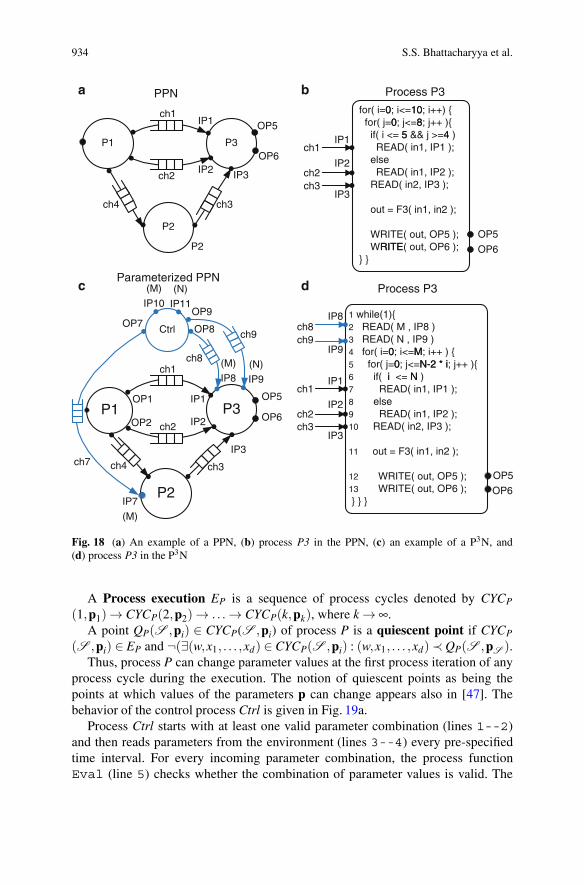
7.4 Parameterized Polyhedral Process Networks
Parameters that appear in a SANLP program are static. In a DANLP, parameters canbe dynamic. A polyhedral process network [73] that is input–output equivalent tosuch a DANLP program is, then, a parameterized polyhedral process network calledP3N in [78].
Remark. There are two assumptions here. First, dynamic conditions, dynamic loopbounds and dynamic while-loops are left out to focus only on dynamic parameters.Second, values of the dynamic parameters are obtained from the environment.
The formal definition of a P3N is given in [78], and is only slightly different fromthe definition given in [73]. Although the consistency of a P3N has to be checkedat run-time, still some analysis can be done at compile-time. A simple example of aP3N is shown in Fig. 18.
Figure 18a is a static PPN, process P3 of which is shown in Fig. 18b. Figure 18cis a P3N version of the PPN in Fig. 18a. Process P3 of the P3N in Fig. 18c is shownin Fig. 18d. The PPN and the P3N have the same dataflow topology. Processes P2and P3 in the P3N in Fig. 18c are reconfigured by two parameters M and N whosevalues are updated from the environment at run-time using process Ctrl and FIFOchannels ch7, ch8, and ch9. The P3N shown in Fig. 18c may be derived from asequential program, yet it can also be constructed from library elements as in [31].
Recall from [73] that a parametric polyhedron P(p) is defined asP(p) = {(w,x1, . . . ,xd)∈Qd+1 | A ·(w,x1, . . . ,xd)
T ≥ B ·p+b}with A ∈Zm×d ,B∈Zm×n and c ∈ Zm. For nested loop programs, w is to be interpreted as the one-dimensional while(1) index, and d as the depth of a loop nest. For a particularvalue of w the polyhedron gets closed, i.e., it becomes a polytope. The parametervector p is bounded by a polytope Pp = {p ∈Qn | C ·p ≥ d}.
The domain DP of a process is defined as the set of all integral points in itsunderlying parametric polyhedron, i.e., DP = PP(p)∩Zd+1. The domains DIP andDOP of an input port IP and an output port OP, respectively, of a process aresubdomains of the domain of that process.
The following four notions play a role in the operational semantics of a P3N:
• Process iteration.• Process cycle.• Process execution.• Quiescent point.
A process iteration of process P is a point (w,x1, . . . ,xd)∈ DP, where the followingoperations are performed sequentially: reading a token from each IP for which(w,x1, . . . ,xd) ∈ DIP, executing process function FP, and writing a token to eachOP for which (w,x1, . . . ,xd) ∈ DOP.
A process cycle CYCP(S ,p)⊂ DP is the set of lexicographically ordered points∈DP for a particular value of w=S ∈Z+. The lexical ordering is typically imposedby a loop nest.
934 S.S. Bhattacharyya et al.
for( i=00; i<=1100; i++) { for( j=00; j<=88; j++ ){ if( i <= 55 && j >=44 ) READ( in1, IP1 ); else READ( in1, IP2 ); READ( in2, IP3 );
out = F3( in1, in2 );
WRITE( out, OP5 );WRRIITTEE( out, OP6 );
} }
Process P3
P1 P3
P2
ch3
P2
PPN
OP5
P1 P3
P2
ch1
ch4 ch3
(M)
IP10(N)
IP111 while(1){2 READ( M , IP8 )3 READ( N , IP9 )4 for( i=00; i<=MM; i++ ) { 5 for( j=00; j<=NN--22 ** ii; j++ ){6 if( ii <= NN ) 7 READ( in1, IP1 );8 else 9 READ( in1, IP2 );10 READ( in2, IP3 );
11 out = F3( in1, in2 );
12 WRITE( out, OP5 );13 WRITE( out, OP6 ); } } }
Process P3
ch2
ch1
OP5
ch9ch8
OP1 IP1
ch7
OP6
OP6
Parameterized PPN
OP5
Ctrl
OP6
ch4
OP5
OP6`
IP3
ch8
ch9
IP1
IP3
(M)
IP8(N)
IP9
IP2ch2 ch3
IP8
IP9
IP1
IP3
IP2
OP2
IP7
(M)
OP8
OP9OP7
ch2
ch1
IP2 ch2
ch1
ch3
IP1
IP3
IP2
a b
c d
Fig. 18 (a) An example of a PPN, (b) process P3 in the PPN, (c) an example of a P3N, and(d) process P3 in the P3N
A Process execution EP is a sequence of process cycles denoted by CYCP
(1,p1)→ CYCP(2,p2)→ . . .→ CYCP(k,pk), where k → ∞.A point QP(S ,pi) ∈ CYCP(S ,pi) of process P is a quiescent point if CYCP
(S ,pi) ∈ EP and ¬(∃(w,x1, . . . ,xd) ∈ CYCP(S ,pi) : (w,x1, . . . ,xd)≺ QP(S ,pS ).Thus, process P can change parameter values at the first process iteration of any
process cycle during the execution. The notion of quiescent points as being thepoints at which values of the parameters p can change appears also in [47]. Thebehavior of the control process Ctrl is given in Fig. 19a.
Process Ctrl starts with at least one valid parameter combination (lines 1--2)and then reads parameters from the environment (lines 3--4) every pre-specifiedtime interval. For every incoming parameter combination, the process functionEval (line 5) checks whether the combination of parameter values is valid. The
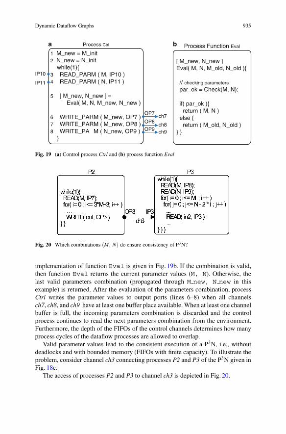
Dynamic Dataflow Graphs 935
1 M_new = M_init2 N_new = N_init while(1){3 READ_PARM ( M, IP10 )4 READ_PARM ( N, IP11 )
5 [ M_new, N_new ] = Eval( M, N, M_new, N_new )
6 WRITE_PARM ( M_new, OP7 )7 WRITE_PARM ( M_new, OP8 ) 8 WRITE_PA
a b
M ( N_new, OP9 ) }
Process Ctrl
[ M_new, N_new ] Eval( M, N, M_old, N_old ){
// checking parameters
par_ok = Check(M, N);
if( par_ok ){ return ( M, N ) else { return ( M_old, N_old ) } }
Process Function Eval
IP10
IP11
ch8
ch7OP7
OP9
OP8
ch9
Fig. 19 (a) Control process Ctrl and (b) process function Eval
Fig. 20 Which combinations (M, N) do ensure consistency of P3N?
implementation of function Eval is given in Fig. 19b. If the combination is valid,then function Eval returns the current parameter values (M, N). Otherwise, thelast valid parameters combination (propagated through M new, N new in thisexample) is returned. After the evaluation of the parameters combination, processCtrl writes the parameter values to output ports (lines 6–8) when all channelsch7, ch8, and ch9 have at least one buffer place available. When at least one channelbuffer is full, the incoming parameters combination is discarded and the controlprocess continues to read the next parameters combination from the environment.Furthermore, the depth of the FIFOs of the control channels determines how manyprocess cycles of the dataflow processes are allowed to overlap.
Valid parameter values lead to the consistent execution of a P3N, i.e., withoutdeadlocks and with bounded memory (FIFOs with finite capacity). To illustrate theproblem, consider channel ch3 connecting processes P2 and P3 of the P3N given inFig. 18c.
The access of processes P2 and P3 to channel ch3 is depicted in Fig. 20.

936 S.S. Bhattacharyya et al.
Consistency requires that, for each corresponding process cycle of both processesCYCP2(i,Mi) and CYCP3(i,Mi,Ni), the number of tokens produced by process P2 tochannel ch3 must be equal to the number of tokens consumed by process P3 fromchannel ch3. For example, if (M,N) = (7,8), P2 produces 25 tokens to ch3 and P3consumes 25 tokens from the same channel after one corresponding process cycleof both processes. It can be verified that P2 produces 13 tokens to ch3 while P3requires 20 tokens from it in a corresponding process cycle when (M,N) = (3,7).Thereby, in order to complete one execution cycle of P3 in this case, it will read datafrom ch3 which will be produced during the next execution cycle of P2. Evidentlythis leads to an incorrect execution of the P3N. From this example, it is clearlyseen that the incoming values of (M,N) must satisfy certain relation to ensure theconsistent execution of the P3N.
Although the consistency of a P3N has to be checked at run-time, still someanalysis can be done at design-time. This is because input ports and output ports ofa process cycle are parametric polytopes. The number of points in a port domainequals the number of tokens that will be written to a channel or read from a channeldepending on whether the port is an output port or an input port, respectively. Thecondition |DCYC
OP | = |DCYCIP | can be checked by comparing the number of points
in both port domains. The counting problem can be solved in polynomial timeusing the Barvinok library [73, 75]. In general the number of points in domainDX = PX(p)∩Zd+1, where X stand for either a process P, an input port IP, oran output port OP, is a set of quasi-polynomials [73].
For the example shown in Fig. 20, the difference |DCYCOP | − |DCYC
IP | is,
{(1+N +N ·M−M2)− (3M+4) = 0 if (M,N) ∈C1(1+ 3
4 N + 14 N2 + 1
4 N − 14 · {0,1}N)− (3M+4) = 0 if (M,N) ∈C2
where C1 = {(M,N) ∈ Z2 | M ≤ N ∧ 2M ≥ 1+N}, C2 = {(M,N) ∈ Z2 | 2M ≤N}, and {0,1}N is a periodic coefficient with period 2.8 In this example, if therange of the parameters is 0 ≤ M,N ≤ 100, then there are only ten valid parametercombinations. If 0≤ M,N ≤ 1,000, then there are 34 valid parameter combinations,and if 0 ≤ M,N ≤ 10,000, then the number of valid combinations is 114.
The symbolic subtraction of the quasi-polynomials can result in constant zero,non-zero constant, or a quasi-polynomial. In the first case, consistency is alwayspreserved for all parameters within the range. In the second case, all parameterswithin the range are invalid, because they violate the consistency condition. Inthe third case, a quasi-polynomial remains, and only some parameter combinationswithin the range are valid for the consistency condition. The equations can be solvedat design time, and all valid parameter combinations are put in a table which isstored in a function Check. At run-time, the control process only propagates thoseincoming parameter combinations that match an entry in the table. Alternatively,function Check evaluates the difference between the two quasi-polynomials against
8{0,1}N is 0 or 1 depending on whether N is even or odd, respectively.

Dynamic Dataflow Graphs 937
zero with incoming parameter values at run-time. When using a table, the executiontime of the P3N is almost equal to the execution time of the corresponding PPN.On the other hand, evaluation the polynomials at run-time overlaps the dataflowprocessing. For medium and high workloads (execution latency of the processes)the overhead is negligible. See [78] for further details.
8 The Stream-Based Function Model
The active entities in dataflow graphs are pure functions, embedded in Actors. Indataflow (polyhedral and parameterized polyhedral) process networks, the activeentities encompass state and pure functions. They are called Processes. Actors andprocesses are specified in a host language like C, C++ or Java, by convention.
Remark. For reasons of convenience, the active entities in dataflow graphs anddataflow networks will in this section be called actors, whether they are void ofstate, encompass a single thread of control, or are processes. Thus static dataflowgraphs [31], dynamic dataflow graphs, polyhedral process [73] and Sect. 7.4, andKahn process networks [21] will collectively be referred to as Dataflow Actor Net-works (DFAN). They obey the Kahn coordination semantics, possibly augmentedwith actor firing rules, annotated with deadlock free minimal FIFO buffer capacities,and one or more global schedules associated with them.
This section deals with a parallel model for actors, called Stream-based func-tion (SBF) in [38] SBF is appealing when it comes to implementing a DFAN ina heterogeneous multiprocessor execution platform that consists of a number ofcomputational elements (processors), and a communication, synchronization, andstorage infrastructure. This requires a mapping that relates an untimed applicationmodel and a timed architecture model together: Actors are assigned to processors(both of type ISA and dedicated), FIFO channels are logically embedded in—often distributed—memory, and DFAN communication primitives and protocolsare transformed to platform specific communication primitives and protocols. Thespecification of platform processors and DFAN actors may be quite different.
The SBF can serve as an intermediate specification between the conventionalDFAN actor specification, and a variety of computational elements in the executionplatform.
8.1 The Stream-Based Function Actor
The SBF is composed of a set of functions, called function repertoire, a transitionand selection function, called controller, and a combined function and data state,called private memory. The controller selects a function from the function repertoirethat is associated with a current function state, and makes a transition to the next

938 S.S. Bhattacharyya et al.
fb
faRead Ports
Enable Signal
Output Buffer0
Write PortStateInput Buffer0
Input Buffer1Controller
Fig. 21 A simple SBF actor
function state. A selected function is enabled when all its input arguments can beread, and all its results can be written; it is blocked otherwise. A selected non-blocked function must evaluate or fire. Arguments and results are called input tokensand output tokens, respectively.
An actor operates on sequences of tokens, streams or signals, as a result of arepetitive enabling and firing of functions from the function repertoire. Tokens areread from external ports and/or loaded from private memory, and are written toexternal ports and/or stored in private memory. The external ports connect to FIFOchannels through which actors communicate point-to-point.
Figure 21 depicts an illustrative stream-based function (SBF) actor. Its functionrepertoire is P = { finit , fa, fb}. The two read ports, and the single write port connectto two input and one output FIFO channels, respectively. P contains at least aninitialization function finit , and is a finite set of functions. The functions in P must beselected in a mutual exclusive order. That order depends on the controller’s selectionand transition function. The private memory consists of a function state part, and adata state part that do not intersect.
8.2 The Formal Model
If C denotes the SBF actor’s function state space, and if D denotes its data statespace, then the actor’s state space S is the Cartesian product of C and D,
S =C×D, C∩D = /0. (2)
Let c ∈ C be the current function state. From c, the controller selects a functionand makes a function state transition by activating its selection function μ andtransition function ω as follows,
μ : C → P, μ(c) = f , (3)
ω : C×D →C, ω(c,d) = c′. (4)

Dynamic Dataflow Graphs 939
The evaluation of the combined functions μ and ω is instantaneous. Thecontroller cannot change the content of C; it can only observe it. The transitionfunction allows for a dynamic behavior as it involves the data state space D.When the transition function is only a map from C to C, then the trajectory ofselected functions will be static (see [31, 73]). Assuming that the DFAN does notdeadlock, and that its input streams are not finite, the controller will repeatedlyinvoke functions from the function repertoire P in an endless firing of functions,
finitμ(ω(S))−→ fa
μ(ω(S))−→ fbμ(ω(S))−→ . . . fx
μ(ω(S))−→ . . . (5)
Such a behavior is called a Fire-and-Exit behavior. It is quite different from athreaded approach in that all synchronization points are explicit. The role of thefunction finit in (5) is crucial. This function has to provide the starting currentfunction state cinit ∈C
cinit = finit (channela . . .channelz). (6)
It evaluates first and only once, and it may read tokens from one or more externalports to return the starting current function state.
The SBF model is reminiscent of the Applicative State Transition (AST) node inthe systolic array model of computation [34] introduced by Annevelink [1], after theApplicative State Transition programming model proposed by Backus [2]. The ASTnode, like the SBF actor, comprises a function repertoire, a selection function μ , anda transition function ω . However, the AST node does not have a private memory,and the initial function state cinit is read from a unique external channel. Moreover,AST nodes communicate through register channels. The SBF actor model is alsoreminiscent of the CAL, which is discussed in Sect. 3.
Clearly, the actors in decidable dataflow models [31] and the multidimensionaldataflow models [37], and the processes in polyhedral precess networks [73] andKahn process networks [21] are special cases of the SBF actor. Analysis is stillpossible in case the SBF-based DFAN originates from weakly dynamic nested loopprograms, see Sect. 7.1, Dynloop programs, see Sect. 7.2, WLAP programs, seeSect. 7.3, and some parameterized polyhedral process networks, see Sect. 7.4.
Actors in dataflow actor networks communicate point to point over FIFObuffered channels. Conceptually, buffer capacities are unlimited, and actors syn-chronize by means of a blocking read protocol: an actor that attempts to readtokens from a specific channel will block whenever that channel is empty. Writingtokens will always proceed. Of course, channel FIFO capacities are not unlimitedin practice, so that a mapped DFAN does have a blocking write protocol as well:an actor that attempts to write tokens to a specific channel will block wheneverthat channel is full. A function [c,d] = f (a,b) has to bind to input ports px and py,respectively, when the function has to receive its arguments a and b, in this order.Similarly, that function has to bind to ports qx and qy, respectively, when ports qx
and qy are to receive results c and d, in this order.

940 S.S. Bhattacharyya et al.
In the SBF actor, the controller’s selection function μ selects both a functionfrom the function repertoire and the corresponding input and output ports. Note thata function that is selected from the function repertoire may read arguments and writeresults from non-unique input ports and to non-unique output ports, respectively, asis also the case with polyhedral process networks [73].
This allows to separate function selection and binding, so that reading, executing,and writing can proceed in a pipelined fashion. Although standard blocking readand blocking write synchronization is possible, the SBF actor allows for a moregeneral deterministic dynamic approach. In this approach, the actor behavior isdivided into a channel checking part and a scheduling part. See also Sect. 5. In thechannel checking part, channels are visited without empty or full channel blocking.A visited input channel Cin returns a Cin.1 signal when the channel is not empty, anda Cin.0 signal when the channel is empty. And similarly for output channels. Thesesignals indicate whether or not a particular function from the function repertoirecan fire. In the scheduling part, a function can only be invoked when the channelchecking signals allow it to fire. If not, then the function will not be invoked. Asa consequence, the actor is blocked. Clearly channel checking and scheduling canproceed in parallel.
9 Summary
This chapter, has reviewed several DSP-oriented dataflow models of computa-tion that are oriented towards representing dynamic dataflow behavior. As signalprocessing systems are developed and deployed for more complex applications,exploration of such generalized dataflow modeling techniques is of increasingimportance. This chapter has complemented the discussion in [31], which focuseson the relatively mature class of decidable dataflow modeling techniques, and buildson the dynamic dataflow principles introduced in certain specific forms [15, 21].
Acknowledgements In this work, Bhattacharyya has been supported in part by the US Air ForceOffice of Scientific Research. The authors also thank Marc Geilen ([email protected]) andSander Stuijk ([email protected]), both from the Eindhoven University of Technology, for theircontribution to Sect. 6.
References
1. Annevelink, J.: HIFI: A design method for implementing signal processing algorithms onVLSI processor arrays. Ph.D. thesis, Delft University of Technology, Department of ElecticalEngineering, Delft, The Netherlands (1988)
2. Backus, J.: Can programming be liberated from the von Neumann style? A functional style andits algebra of programs. Communications of the ACM 21(8), 613–641 (1978)

Dynamic Dataflow Graphs 941
3. Bekooij, M., Hoes, R., Moreira, O., Poplavko, P., Pastrnak, M., Mesman, B., Mol, J., Stuijk, S.,Gheorghita, V., van Meerbergen, J.: Dataflow analysis for real-time embedded multiprocessorsystem design. In: P. van der Stok (ed.) Dynamic and Robust Streaming in and betweenConnected Consumer-Electronic Devices, pp. 81–108. Springer (2005)
4. Benabderrahmane, M.W., Pouchet, L.N., Cohen, A., Bastoul, C.: The polyhedral model is morewidely applicable than you think. In: Proc. International Conference on Compiler Construction(ETAPS CC’10). Paphos, Cyprus (2010)
5. Berg, H., Brunelli, C., Lucking, U.: Analyzing models of computation for software definedradio applications. In: Proceedings of the International Symposium on System-on-Chip (2008)
6. Bhattacharya, B., Bhattacharyya, S.S.: Parameterized dataflow modeling for DSP systems.IEEE Transactions on Signal Processing 49(10), 2408–2421 (2001)
7. Bhattacharyya, S.S., Buck, J.T., Ha, S., Lee, E.A.: Generating compact code from dataflowspecifications of multirate signal processing algorithms. IEEE Transactions on Circuits andSystems — I: Fundamental Theory and Applications 42(3), 138–150 (1995)
8. Bhattacharyya, S.S., Eker, J., Janneck, J.W., Lucarz, C., Mattavelli, M., Raulet, M.: Overviewof the MPEG reconfigurable video coding framework. Journal of Signal Processing Systems(2010). DOI:10.1007/s11265-009-0399-3
9. Bhattacharyya, S.S., Leupers, R., Marwedel, P.: Software synthesis and code generation forDSP. IEEE Transactions on Circuits and Systems — II: Analog and Digital Signal Processing47(9), 849–875 (2000)
10. Bijlsma, T., Bekooij, M.J.G., Smit, G.J.M.: Inter-task communication via overlapping read andwrite windows for deadlock-free execution of cyclic task graphs. In: Proceedings SAMOS’09,pp. 140–148. Samos, Greece (2009)
11. Buck, J.T.: Scheduling dynamic dataflow graphs with bounded memory using the token flowmodel. Ph.D. thesis, Department of Electrical Engineering and Computer Sciences, Universityof California at Berkeley (1993)
12. Collard, J.F.: Automatic parallelization of while-loops using speculative execution. Int. J.Parallel Program. 23(2), 191–219 (1995)
13. Deprettere, E.F., Rijpkema, E., Kienhuis, B.: Translating imperative affine nested loopprograms to process networks. In: E.F. Deprettere, J. Teich, S. Vassiliadis (eds.) EmbeddedProcessor Design Challenges, LNCS 2268, pp. 89–111. Springer, Berlin (2002)
14. Eker, J., Janneck, J.W.: CAL language report, language version 1.0 — document edition 1.Tech. Rep. UCB/ERL M03/48, Electronics Research Laboratory, University of California atBerkeley (2003)
15. Falk, J., Haubelt, C., Zebelein, C., Teich, J.: Integrated modeling using finite state machines anddataflow graphs. In: S.S. Bhattacharyya, E.F. Deprettere, R. Leupers, J. Takala (eds.) Handbookof Signal Processing Systems, second edn. Springer (2013)
16. Feautrier, P.: Dataflow analysis of scalar and array references. Int. Journal of ParallelProgramming 20(1), 23–53 (1991)
17. Feautrier, P.: Automatic parallelization in the polytope model. In: The Data Parallel Program-ming Model, pp. 79–103 (1996)
18. Feautrier, P., Collard, J.F.: Fuzzy array dataflow analysis. Tech. rep., Ecole Normale Superieurede Lyon (1994). ENS-Lyon/LIP No 94-21
19. Gao, G.R., Govindarajan, R., Panangaden, P.: Well-behaved programs for DSP computation.In: Proceedings of the International Conference on Acoustics, Speech, and Signal Processing(1992)
20. Geilen, M.: Synchronous dataflow scenarios. ACM Trans. Embed. Comput. Syst. 10(2),16:1–16:31 (2011)
21. Geilen, M., Basten, T.: Kahn process networks and a reactive extension. In: S.S. Bhattacharyya,E.F. Deprettere, R. Leupers, J. Takala (eds.) Handbook of Signal Processing Systems, secondedn. Springer (2013)
22. Geilen, M.C.W., Basten, T., Theelen, B.D., Otten, R.J.H.M.: An algebra of pareto points.Fundamenta Informaticae 78(1), 35–74 (2007)

942 S.S. Bhattacharyya et al.
23. Geilen, M.C.W., Falk, J., Haubelt, C., Basten, T., Theelen, B.D., Stuijk, S.: Performanceanalysis of weakly-consistent scenario-aware dataflow graphs. Tech. Rep. ESR-2011-03,Eindhoven University of Technology (2011)
24. Geilen, M., Stuijk, S.: Worst-case performance analysis of synchronous dataflow scenarios.In: Proceedings of the eighth IEEE/ACM/IFIP international conference on hardware/softwarecodesign and system synthesis, CODES/ISSS ’10, pp. 125–134. ACM, New York, NY, USA(2010)
25. Geuns, S., Bijlsma, T., Corporaal, H., Bekooij, M.: Parallelization of while loops in nested loopprograms for shared-memory multiprocessor systems. In: Proc. Int. Conf. Design, Automationand Test in Europe (DATE’11). Grenoble, France (2011)
26. Gheorghita, S.V., Stuijk, S., Basten, T., Corporaal, H.: Automatic scenario detection for im-proved WCET estimation. In: Proceedings of the 42nd annual Design Automation Conference,DAC ’05, pp. 101–104. ACM, New York, NY, USA (2005)
27. Girault, A., Lee, B., Lee, E.: Hierarchical finite state machines with multiple concurrencymodels. Computer-Aided Design of Integrated Circuits and Systems, IEEE Transactions on18(6), 742 –760 (1999)
28. Griebl, M., Collard, J.F.: Generation of Synchronous Code for Automatic Parallelization ofwhile-loops. EURO-PAR’95, Springer-Verlag LNCS, number 966, pp. 315–326 (1995)
29. Griebl, M., Lengauer, C.: A communication scheme for the distributed execution of loop nestswith while loops. Int. J. Parallel Programming 23 (1995)
30. Gu, R., Janneck, J., Raulet, M., Bhattacharyya, S.S.: Exploiting statically schedulable regionsin dataflow programs. In: Proceedings of the International Conference on Acoustics, Speech,and Signal Processing, pp. 565–568. Taipei, Taiwan (2009)
31. Ha, S., Oh, H.: Decidable dataflow models for signal processing: Synchronous dataflow and itsextensions. In: S.S. Bhattacharyya, E.F. Deprettere, R. Leupers, J. Takala (eds.) Handbook ofSignal Processing Systems, second edn. Springer (2013)
32. Haykin, S.: Adaptive Filter Theory. Prentice Hall (1996)33. Hermanns, H.: Interactive Markov chains: and the quest for quantified quality. Springer-Verlag,
Berlin, Heidelberg (2002)34. Hu, Y.H., Kung, S.Y.: Systolic arrays. In: S.S. Bhattacharyya, E.F. Deprettere, R. Leupers,
J. Takala (eds.) Handbook of Signal Processing Systems, second edn. Springer (2013)35. Kahn, G.: The semantics of a simple language for parallel programming. In: Proc. of
Information Processing (1974)36. Kee, H., Wong, I., Rao, Y., Bhattacharyya, S.S.: FPGA-based design and implementation
of the 3GPP-LTE physical layer using parameterized synchronous dataflow techniques. In:Proceedings of the International Conference on Acoustics, Speech, and Signal Processing, pp.1510–1513. Dallas, Texas (2010)
37. Keinert, J., Deprettere, E.F.: Multidimensional dataflow graphs. In: S.S. Bhattacharyya, E.F.Deprettere, R. Leupers, J. Takala (eds.) Handbook of Signal Processing Systems, second edn.Springer (2013)
38. Kienhuis, B., Deprettere, E.F.: Modeling stream-based applications using the SBF model ofcomputation. Journal of Signal Processing Systems 34(3), 291–299 (2003)
39. Kienhuis, B., Rijpkema, E., Deprettere, E.F.: Compaan: Deriving Process Networks fromMatlab for Embedded Signal Processing Architectures. In: Proc. 8th International Workshopon Hardware/Software Codesign (CODES’2000). San Diego, CA, USA (2000)
40. Ko, M., Zissulescu, C., Puthenpurayil, S., Bhattacharyya, S.S., Kienhuis, B., Deprettere,E.: Parameterized looped schedules for compact representation of execution sequences inDSP hardware and software implementation. IEEE Transactions on Signal Processing 55(6),3126–3138 (2007)
41. Lin, Y., Choi, Y., Mahlke, S., Mudge, T., Chakrabarti, C.: A parameterized dataflow languageextension for embedded streaming systems. In: Proceedings of the International Symposiumon Systems, Architectures, Modeling and Simulation, pp. 10–17 (2008)
42. Mattavelli, M., Raulet, M., Janneck, J.W.: MPEG reconfigurable video coding. In: S.S.Bhattacharyya, E.F. Deprettere, R. Leupers, J. Takala (eds.) Handbook of Signal ProcessingSystems, second edn. Springer (2013)

Dynamic Dataflow Graphs 943
43. Moreira, O.: Temporal analysis and scheduling of hard real-time radios running on a multi-processor. Ph.D. thesis, Eindhoven University of Technology (2012)
44. Nadezhkin, D., Nikolov, H., Stefanov, T.: Translating affine nested-loop programs withdynamic loop bounds into polyhedral process networks. In: ESTImedia, pp. 21–30 (2010)
45. Nadezhkin, D., Stefanov, T.: Automatic derivation of polyhedral process networks from while-loop affine programs. In: ESTImedia, pp. 102–111 (2011)
46. Neuendorffer, S., Lee, E.: Hierarchical reconfiguration of dataflow models. In: Proceedings ofthe International Conference on Formal Methods and Models for Codesign (2004)
47. Neuendorffer, S., Lee, E.: Hierarchical reconfiguration of dataflow models. In: Proc. ofMEMOCODE, pp. 179–188 (2004)
48. Nikolov, H., Stefanov, T., Deprettere, E.: Systematic and automated multi-processor systemdesign, programming, and implementation. IEEE Transactions on Computer-Aided Design27(3), 542–555 (2008)
49. Plishker, W., Sane, N., Bhattacharyya, S.S.: A generalized scheduling approach for dynamicdataflow applications. In: Proceedings of the Design, Automation and Test in Europe Confer-ence and Exhibition, pp. 111–116. Nice, France (2009)
50. Plishker, W., Sane, N., Bhattacharyya, S.S.: Mode grouping for more effective generalizedscheduling of dynamic dataflow applications. In: Proceedings of the Design AutomationConference, pp. 923–926. San Francisco (2009)
51. Plishker, W., Sane, N., Kiemb, M., Anand, K., Bhattacharyya, S.S.: Functional DIF for rapidprototyping. In: Proceedings of the International Symposium on Rapid System Prototyping,pp. 17–23. Monterey, California (2008)
52. Poplavko, P., Basten, T., van Meerbergen, J.L.: Execution-time prediction for dynamicstreaming applications with task-level parallelism. In: DSD, pp. 228–235 (2007)
53. Raman, E., Ottoni, G., Raman, A., Bridges, M.J., August, D.I.: Parallel-stage decoupledsoftware pipelining. In: Proc. 6th annual IEEE/ACM international symposium on Codegeneration and optimization, pp. 114–123 (2008)
54. Rauchwerger, L., Padua, D.: Parallelizing while loops for multiprocessor systems. In: InProceedings of the 9th International Parallel Processing Symposium (1995)
55. Rijpkema, E., Deprettere, E., Kienhuis, B.: Deriving process networks from nested loopalgorithms. Parallel Processing Letters 10(2), 165–176 (2000)
56. Roquier, G., Wipliez, M., Raulet, M., Janneck, J.W., Miller, I.D., Parlour, D.B.: Automaticsoftware synthesis of dataflow program: An MPEG-4 simple profile decoder case study. In:Proceedings of the IEEE Workshop on Signal Processing Systems (2008)
57. Saha, S., Puthenpurayil, S., Bhattacharyya, S.S.: Dataflow transformations in high-levelDSP system design. In: Proceedings of the International Symposium on System-on-Chip,pp. 131–136. Tampere, Finland (2006)
58. Shlien, S.: Guide to MPEG-1 audio standard. Broadcasting, IEEE Transactions on 40(4),206 –218 (1994)
59. Shojaei, H., Ghamarian, A., Basten, T., Geilen, M., Stuijk, S., Hoes, R.: A parameterizedcompositional multi-dimensional multiple-choice knapsack heuristic for CMP run-time man-agement. In: Design Automation Conf., DAC 09, Proc., pp. 917–922. ACM (2009)
60. Stefanov, T., Deprettere, E.: Deriving process networks from weakly dynamic applicationsin system-level design. In: Proc. IEEE-ACM-IFIP International Conference on Hardware/-Software Codesign and System Synthesis (CODES+ISSS’03), pp. 90–96. Newport Beach,California, USA (2003)
61. Stefanov, T., Kienhuis, B., Deprettere, E.: Algorithmic transformation techniques for efficientexploration of alternative application instances. In: Proc. 10th Int. Symposium on Hardware/-Software Codesign (CODES’02), pp. 7–12. Estes Park CO, USA (2002)
62. Stuijk, S., Geilen, M., Basten, T.: SDF3: SDF For Free. In: Application of Concurrency toSystem Design, 6th International Conference, ACSD 2006, Proceedings, pp. 276–278. IEEEComputer Society Press, Los Alamitos, CA, USA (2006). DOI 10.1109/ACSD.2006.23. URLhttp://www.es.ele.tue.nl/sdf3
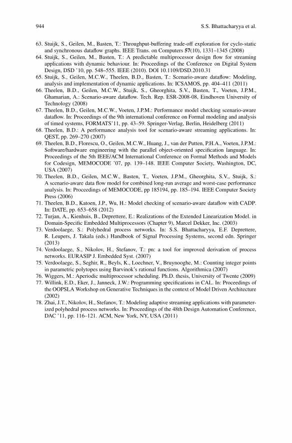
944 S.S. Bhattacharyya et al.
63. Stuijk, S., Geilen, M., Basten, T.: Throughput-buffering trade-off exploration for cyclo-staticand synchronous dataflow graphs. IEEE Trans. on Computers 57(10), 1331–1345 (2008)
64. Stuijk, S., Geilen, M., Basten, T.: A predictable multiprocessor design flow for streamingapplications with dynamic behaviour. In: Proceedings of the Conference on Digital SystemDesign, DSD ’10, pp. 548–555. IEEE (2010). DOI 10.1109/DSD.2010.31
65. Stuijk, S., Geilen, M.C.W., Theelen, B.D., Basten, T.: Scenario-aware dataflow: Modeling,analysis and implementation of dynamic applications. In: ICSAMOS, pp. 404–411 (2011)
66. Theelen, B.D., Geilen, M.C.W., Stuijk, S., Gheorghita, S.V., Basten, T., Voeten, J.P.M.,Ghamarian, A.: Scenario-aware dataflow. Tech. Rep. ESR-2008-08, Eindhoven University ofTechnology (2008)
67. Theelen, B.D., Geilen, M.C.W., Voeten, J.P.M.: Performance model checking scenario-awaredataflow. In: Proceedings of the 9th international conference on Formal modeling and analysisof timed systems, FORMATS’11, pp. 43–59. Springer-Verlag, Berlin, Heidelberg (2011)
68. Theelen, B.D.: A performance analysis tool for scenario-aware streaming applications. In:QEST, pp. 269–270 (2007)
69. Theelen, B.D., Florescu, O., Geilen, M.C.W., Huang, J., van der Putten, P.H.A., Voeten, J.P.M.:Software/hardware engineering with the parallel object-oriented specification language. In:Proceedings of the 5th IEEE/ACM International Conference on Formal Methods and Modelsfor Codesign, MEMOCODE ’07, pp. 139–148. IEEE Computer Society, Washington, DC,USA (2007)
70. Theelen, B.D., Geilen, M.C.W., Basten, T., Voeten, J.P.M., Gheorghita, S.V., Stuijk, S.:A scenario-aware data flow model for combined long-run average and worst-case performanceanalysis. In: Proceedings of MEMOCODE, pp 185194, pp. 185–194. IEEE Computer SocietyPress (2006)
71. Theelen, B.D., Katoen, J.P., Wu, H.: Model checking of scenario-aware dataflow with CADP.In: DATE, pp. 653–658 (2012)
72. Turjan, A., Kienhuis, B., Deprettere, E.: Realizations of the Extended Linearization Model. inDomain-Specific Embedded Multiprocessors (Chapter 9), Marcel Dekker, Inc. (2003)
73. Verdoolaege, S.: Polyhedral process networks. In: S.S. Bhattacharyya, E.F. Deprettere,R. Leupers, J. Takala (eds.) Handbook of Signal Processing Systems, second edn. Springer(2013)
74. Verdoolaege, S., Nikolov, H., Stefanov, T.: pn: a tool for improved derivation of processnetworks. EURASIP J. Embedded Syst. (2007)
75. Verdoolaege, S., Seghir, R., Beyls, K., Loechner, V., Bruynooghe, M.: Counting integer pointsin parametric polytopes using Barvinok’s rational functions. Algorithmica (2007)
76. Wiggers, M.: Aperiodic multiprocessor scheduling. Ph.D. thesis, University of Twente (2009)77. Willink, E.D., Eker, J., Janneck, J.W.: Programming specifications in CAL. In: Proceedings of
the OOPSLA Workshop on Generative Techniques in the context of Model Driven Architecture(2002)
78. Zhai, J.T., Nikolov, H., Stefanov, T.: Modeling adaptive streaming applications with parameter-ized polyhedral process networks. In: Proceedings of the 48th Design Automation Conference,DAC ’11, pp. 116–121. ACM, New York, NY, USA (2011)