Dynamic Data-Driven Avionics Systems:

Inferring Failure Modes from Data Streams

Shigeru Imai, Alessandro Galli, and Carlos A. Varela

Rensselaer Polytechnic Institute, Troy, NY 12180, USA{imais,gallia}@.rpi.edu, cvarela@cs.rpi.edu

AbstractDynamic Data-Driven Avionics Systems (DDDAS) embody ideas from the Dynamic Data-Driven Application Systems paradigm by creating a data-driven feedback loop that analyzesspatio-temporal data streams coming from aircraft sensors and instruments, looks for errorsin the data signaling potential failure modes, and corrects for erroneous data when possible.In case of emergency, DDDAS need to provide enough information about the failure to pilotsto support their decision making in real-time. We have developed the PILOTS system, whichsupports data-error tolerant spatio-temporal stream processing, as an initial step to realize theconcept of DDDAS. In this paper, we apply the PILOTS system to actual data from the Tuninter1153 (TU1153) flight accident in August 2005, where the installation of an incorrect fuel sensorled to a fatal accident. The underweight condition suggesting an incorrect fuel indication forTU1153 is successfully detected with 100% accuracy during cruise flight phases. Adding logicalredundancy to avionics through a dynamic data-driven approach can significantly improve thesafety of flight.

Keywords: programming models, spatio-temporal data, data streaming

1 Introduction

Dynamic Data-Driven Avionics Systems (DDDAS) based on the concept of Dynamic Data-Driven Application Systems [1] use sensor data in real-time to enrich computational modelsin order to more accurately predict aircraft performance under partial failures. DDDAS cantherefore support better-informed decision making for pilots and can also be applicable toautonomous unmanned air and space vehicles. As a first step towards realizing DDDAS, we havedeveloped a system called PILOTS (ProgrammIng Language for spatiO-Temporal Streamingapplications) [2, 3, 4] that enables specifying error detection and data correction in spatio-temporal data streams using a highly-declarative programming language. Figure 1 shows aconceptual view of DDDAS. Upon a request from the Avionics Application, the Pre-Processortakes raw data streams from aircraft sensors and then produces homogeneous and correctedstreams. Following data pre-processing, the Avionics Application can constantly compute its

Procedia Computer Science

Volume XXX, 2015, Pages 1–10

ICCS 2015. International Conference On Computational Science

Selection and peer-review under responsibility of the Scientific Programme Committee of ICCS 2015c© The Authors. Published by Elsevier B.V.

1

desired output with the corrected data. Since the Avionics Application controls the aircraftultimately based on the raw data streams from the sensors, we can see that understanding dataerrors to detect potential sensor and instrument failures can significantly augment the envelopeof operations of autonomous flight systems.

��������

��������������

�������������������

������ ��

�������������

������������

�������

�����������

�������

������������������

�����������

����������

������������

����������

�����������

���������

���!����

�� ������

������"�

�� ��

Figure 1: Conceptual view of Dynamic Data-Driven Avionics Systems

PILOTS has been successfully applied to detect the airspeed sensors failure which occurredin the Air France flight 447 accident from its recovered black box data [5]. In this paper, weanalyze the TU1153 flight [6], where the installation of an incorrect fuel sensor led to a fatalaccident. In the AF447 case, we used the relationship between airspeed, ground speed, andwind speed data to infer the pitot tubes failure. In the TU1153 case, we use the relationshipbetween fuel weight, and aircraft performance (airspeed) data.

The rest of the paper is organized as follows. Section 2 describes error signature-basederror detection and correction methods as well as the PILOTS programming language and thearchitecture of its runtime system. Section 3 discusses the design of error signatures and resultsof error detection performance for the TU1153 flight data, and Section 4 describes relatedwork. Finally, we briefly describe future research directions for real-time error-tolerant streamprocessing and conclude the paper in Section 5.

2 Error-Tolerant Spatio-Temporal Data Streaming

2.1 Error Detection and Correction Methods

Error functions An error function is an arbitrary function that computes a numerical valuefrom independently measured input data. It is used to examine the validity of redundant data.If the value of an error function is zero, we normally interpret it as no error in the given data.

The relationship between ground speed (ÝÑvg), airspeed (ÝÑva), and wind speed (ÝÑvw) shown inEquation 1 is visually depicted in Figure 2.

ÝÑvg “ ÝÑva `ÝÑvw. (1)

A vector ÝÑv can be defined by a tuple pv, αq, where v is the magnitude of ÝÑv and α is theangle between ÝÑv and a base vector. Following this expression, ÝÑvg ,ÝÑva, and ÝÑvw are defined aspvg, αgq, pva, αaq, and pvw, αwq respectively. We can compute ÝÑvg by applying trigonometry to4ABC and define an error function as the difference between measured vg and computed vgas follows:

epÝÑvg ,ÝÑva,ÝÑvwq “ |ÝÑvg ´ pÝÑva `ÝÑvwq| “ vg ´a

v2a ` 2vavw cospαa ´ αwq ` v2

w. (2)

The values of input data are assumed to be sampled periodically from corresponding spatio-temporal data streams. Thus, an error function e changes its value as time proceeds and canalso be represented as eptq.

Imai et al.

2

vw

va

αa-α

w

vg

αa

C

A

B

αw

Figure 2: Trigonometry applied to theground speed, airspeed, and wind speed.

Ot

f

...

5

2

f(t)

= t + 2

f(t) =

t +

5

Figure 3: Error signature SI with a linearfunction fptq “ t` k, 2 ď k ď 5.

Error signatures An error signature is a constrained mathematical function pattern thatis used to capture the characteristics of an error function eptq. Using a vector of constantsK “ xk1, . . . , kmy, a function fpt, Kq, and a set of constraint predicates P “ tp1pKq, . . . , plpKqu,the error signature SpK, fpt, Kq, P pKqq is defined as follows:

Spfpt, Kq, P pKqq fi t f | p1pKq ^ ¨ ¨ ¨ ^ plpKqu. (3)

For example, an interval error signature SI can be defined as SI “ Spfpt, Kq, IpK, A, Bqq “t f | a1 ď k1 ď b1, . . . , am ď km ď bmu, where A “ xa1, . . . , amy and B “ xb1, . . . , bmy. Whenfpt, Kq “ t ` k, K “ xky, A “ x2y, and B “ x5y, the error signature SI contains all linearfunctions with slope 1, and crossing the Y-axis at values r2, 5s as shown in Figure 3.

Mode likelihood vectors Given a vector of error signatures xS0, . . . , Sny, we calculateδipSi, tq, the distance between the measured error function eptq and each error signature Si by:

δipSi, tq “ mingptqPSi

ż t

t´ω

|eptq ´ gptq|dt. (4)

where ω is the window size. Note that our convention is to capture “normal” conditions assignature S0. The smaller the distance δi, the closer the raw data is to the theoretical signatureSi. We define the mode likelihood vector as Lptq “ xl0ptq, l1ptq, . . . , lnptqy where each liptq is:

liptq “

#

1, if δiptq “ 0mintδ0ptq,...,δnptqu

δiptq, otherwise.

(5)

Mode estimation Using the mode likelihood vector, the final mode output is estimated asfollows. Observe that for each li P L, 0 ă li ď 1 where li represents the ratio of the likelihoodof signature Si being matched with respect to the likelihood of the best signature. Because ofthe way Lptq is created, the largest element lj will always be equal to 1. Given a thresholdτ P p0, 1q, we check for one likely candidate lj that is sufficiently more likely than its successorlk by ensuring that lk ď τ . Thus, we determine j to be the correct mode by choosing the mostlikely error signature Sj . If j “ 0 then the system is in normal mode. If lk ą τ , then regardlessof the value of k, unknown error mode (´1) is assumed.

Error correction Whether or not a known error mode i is recoverable is problem depen-dent. If there is a mathematical relationship between an erroneous value and other indepen-dently measured values, the erroneous value can be replaced by a new value computed from the

Imai et al.

3

other independently measured values. In the case of the speed example used in Equations 1and 2, if the ground speed vg is detected as erroneous, its corrected value vg can be computed

by the airspeed and wind speed as vg “a

v2a ` 2vavw cospαa ´ αwq ` v2

w.

2.2 Spatio-Temporal Data Stream Processing System

2.2.1 System Architecture

Figure 4 shows the architecture of the PILOTS runtime system, which implements the errordetection and correction methods described in Section 2.1. It consists of three parts: the DataSelection, the Error Analyzer, and the Application Model modules. The Application Modelobtains homogeneous data streams pd11, d

12, . . . , d

1N q from the Data Selection module, and then it

generates outputs (o1, o2, . . . , oM ) and data errors (e1, e2, . . . , eL). The Data Selection moduletakes heterogeneous incoming data streams (d1, d2, . . . , dN ) as inputs. Since this runtime isassumed to be working on moving objects, the Data Selection module is aware of the currentlocation and time. Thus, it returns appropriate values to the Application Model by selecting orinterpolating data in time and location, depending on the data selection method specified in thePILOTS program. The Error Analyzer collects the latest ω error values from the ApplicationModel and keeps analyzing errors based on the error signatures. If it detects a recoverableerror, then it replaces an erroneous input with the corrected one by applying a correspondingerror correction equation. The Application Model computes the outputs based on the correctedinputs produced from the Error Analyzer.

d1 (x, y, z, t)

d2 (x, y, z, t)

dN (x, y, z, t)

...

Outputs

Application

Model

Incoming

Data Streams

Outgoing

Data Streams

o2

o1

...

oM

e2

e1

...

eLErrors

Data

Selection

Request data at a specified rate

d1'

d2'

dN'

Error

Detection

Error Signatures

...

Current

Time

Current

Location S = {S0, S1, …, Sn}

mode ?

Compute likelihood vector

L = <l0, l1, ..., ln>Flag error

unknown or

Error

Correction

recoverable or

Correct data if

recoverable

mode

unrecoverable

no error

Error Analyzer

Corrected Data

Figure 4: Architecture of the PILOTS runtime system.

2.2.2 PILOTS Programming Language

PILOTS is a programming language specifically designed for analyzing spatio-temporal datastreams, which potentially contain erroneous data. Compiled PILOTS programs are designedto run on the runtime system described in Section 2.2.1. Using PILOTS, developers can eas-ily program an application that handles spatio-temporal data streams by writing a high-level(declarative) program specification.

PILOTS application programs must contain inputs and outputs sections. The inputs

section specifies the incoming data streams and how data is to be extrapolated from incomplete

Imai et al.

4

data, typically using declarative geometric criteria (e.g., closest, interpolate, euclidean

keywords). Note that these extrapolations are performed based on the current location andtime of the PILOTS system. The outputs section specifies outgoing data streams to be pro-duced by the application, as a function of the input streams with a given frequency. errors

and signatures sections are optional and can be used to detect errors. Similar to the outputs

section, the errors section specifies an error stream to be produced by the application andto be analyzed by the runtime system to recognize known error patterns as described in thesignatures section. If a detected error is recoverable, output values are computed from cor-rected input data using correction formulas under the correct section (See Figure 7 for anactual PILOTS program example).

3 Analyzing Tuninter 1153 Flight Data

Tuninter 1153 flight (TU1153) was a flight from Bari, Italy to Djerba, Tunisia on August 6th,2005. About an hour after departure, the ATR 72 aircraft ditched into the Mediterranean Seadue to exhaustion of its fuel, killing 16 of 39 people on board (see Figure 5 for the altitudetransition from the accident report [6]). The accident was caused by the installation of anincorrect fuel quantity indicator. That is, a fuel quantity indicator for the smaller ATR 42 wasmistakenly installed, reporting 2150 kg more fuel than actually available. We call this incorrectindicated weight fictitious weight following the accident report.

How could DDDAS have prevented this accident from happening? If all other conditionsare the same between two flights except for the weight, the one with lighter weight would havea higher airspeed. If we could compute expected airspeed from the monitored weight, we cancompare the expected and monitored airspeed to detect if there is a discrepancy between thetwo. Once the system detects the discrepancy, it can warn pilots in an early stage of the flightto prevent the accident. Using this idea, we design a set of error signatures and evaluate it withactual data recorded in the flight data recorder (black box) during the TU1153 flight.

3.1 Error Signatures Design

In the ATR 72 flight crew operating manual [7], there are tables for pilots to estimate cruiseairspeed (knots) under certain conditions of engine power settings, temperature difference tothe International Standard Atmosphere ( ˝C), flight level (feet), and weight (kg) of the aircraft,which are denoted by va, t∆, h, and w respectively. According to the accident report, t∆ “ `10is a reasonable approximation at the time of the accident. By using polynomial regression, we

�

����

�����

�����

�����

�����

� ���� ���� ���� ���� ����

�

�

�

�

�

�

�

�

�

�

�

�

�

���������

�� �� ���

������ ���

Figure 5: Altitude transition of theTU1153 flight.

��

��

��

�

�

�

�

���� ���� ���� ���� ���� ����

�

�

�

�

�

�

�

�

�

�

�

���������

��������

�����

����

���������

�����

����

�� �

Figure 6: Calibration of the error functionby the first cruise phase.

Imai et al.

5

can derive a formula for the estimated airspeed va as follows:

va “ zT ¨ k “

»

—

—

—

—

—

—

–

1wh

w ¨ hw2

h2

fi

ffi

ffi

ffi

ffi

ffi

ffi

fl

T

¨

»

—

—

—

—

—

—

–

6.4869E` 011.4316E´ 026.6730E´ 03´3.7716E´ 07´2.4208E´ 07´1.1730E´ 07

fi

ffi

ffi

ffi

ffi

ffi

ffi

fl

(6)

Using Equation 6, the error function is defined as the difference between the monitored (va)and estimated (va) airspeed:

epva, w, hq “ va ´ va (7)

Figure 6 shows how the error function behaves for the first cruise phase from 2170 to 2370seconds of the flight (see Figure 5 for the two cruise phases observed in the flight) using actualweight. As we can see from the original error plot, error values range from around -4 to -1.5knots. This is expected because there are variables that are not considered in Equation 6 suchas angle of attack, center of gravity, and aircraft tear and wear. To improve the overall fitnessof the error function to the TU1153 data, we can “calibrate” the error function by adding aconstant. In Equation 8, CP1 is a set of data points during the first cruise phase and N is thenumber of data points in CP1 (i.e., N “ |CP1|). This equation is meant to find a constantthat minimizes the squared difference between the error function and the constant itself. Bysubtracting the value of Kcalib “ ´2.59 from Equation 7, we get a new calibrated error functionecalib “ e´Kcalib as shown in the dotted-line of Figure 6.

Kcalib “ argmink

1

N

Nÿ

iPCP1

‖ ei ´ k ‖2“1

N

Nÿ

iPCP1

ei (8)

Since the error function is adjusted to be zero after calibration, naturally we use the errorvalue of zero with small margins to identify a normal condition. For underweight conditions,we set a constraint that will identify 10% discrepancy in weight regardless of the value of τ .Since the 10% weight difference leads to a 4.69 knots difference in airspeed using Equation 6(computed by averaging over w “ 13000 „ 22000 kg at h “ 23000 feet), we use 4.69 as theboundary for the underweight conditions. Note that from Equation 6, the estimated airspeedva monotonically decreases as the weight w increases for fixed h and t∆. Since cruise flightskeep the same altitude, the error should be positive in underweight conditions as occurred inthe TU1153 flight. In summary, we derive the error signature set shown in Table 1.

Table 1: Error signatures for the Tuninter 1153 flight.

Mode Error SignatureFunction Constraints

Normal e “ k ´2 ă k ă 2Underweight e “ k 4.69 ă k

Note that this error signature set is not generally applicable, but specifically adjusted forthe first cruise phase of the TU1153 flight. In a real-world application, we would use more datasets to derive a general error signature set for ATR 72 aircraft; however, we do not have accessto actual ATR 72 flight data including airspeed, weight, altitude, and temperature. Therefore,we create a model for the cruise phases, adjust it to the first cruise phase, and evaluate it withthe second cruise phase.

Imai et al.

6

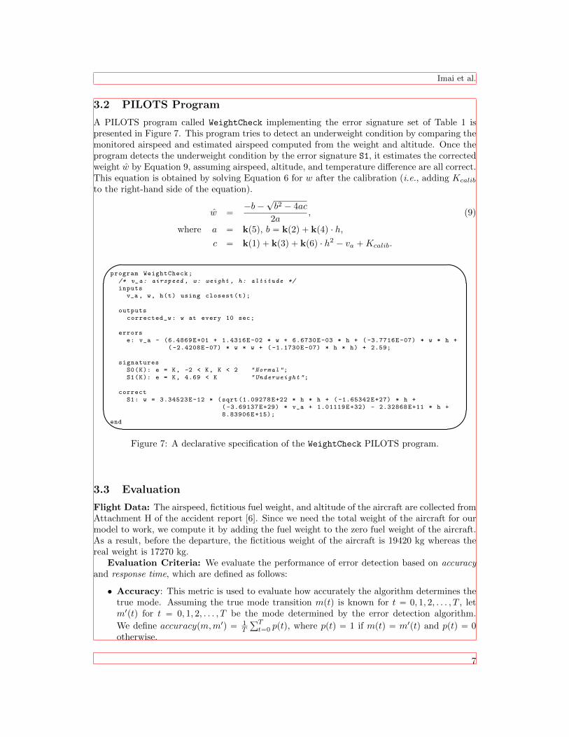
3.2 PILOTS Program

A PILOTS program called WeightCheck implementing the error signature set of Table 1 ispresented in Figure 7. This program tries to detect an underweight condition by comparing themonitored airspeed and estimated airspeed computed from the weight and altitude. Once theprogram detects the underweight condition by the error signature S1, it estimates the correctedweight w by Equation 9, assuming airspeed, altitude, and temperature difference are all correct.This equation is obtained by solving Equation 6 for w after the calibration (i.e., adding Kcalib

to the right-hand side of the equation).

w “´b´

?b2 ´ 4ac

2a, (9)

where a “ kp5q, b “ kp2q ` kp4q ¨ h,

c “ kp1q ` kp3q ` kp6q ¨ h2 ´ va `Kcalib.'

&

$

%

program WeightCheck;/* v_a: airspeed , w: weight , h: altitude */inputs

v_a , w, h(t) using closest(t);

outputscorrected_w: w at every 10 sec;

errorse: v_a - (6.4869E+01 + 1.4316E-02 * w + 6.6730E-03 * h + ( -3.7716E-07) * w * h +

( -2.4208E-07) * w * w + ( -1.1730E-07) * h * h) + 2.59;

signaturesS0(K): e = K, -2 < K, K < 2 "Normal";S1(K): e = K, 4.69 < K " Underweight ";

correctS1: w = 3.34523E-12 * (sqrt (1.09278E+22 * h * h + ( -1.65342E+27) * h +

( -3.69137E+29) * v_a + 1.01119E+32) - 2.32868E+11 * h +8.83906E+15);

end

Figure 7: A declarative specification of the WeightCheck PILOTS program.

3.3 Evaluation

Flight Data: The airspeed, fictitious fuel weight, and altitude of the aircraft are collected fromAttachment H of the accident report [6]. Since we need the total weight of the aircraft for ourmodel to work, we compute it by adding the fuel weight to the zero fuel weight of the aircraft.As a result, before the departure, the fictitious weight of the aircraft is 19420 kg whereas thereal weight is 17270 kg.

Evaluation Criteria: We evaluate the performance of error detection based on accuracyand response time, which are defined as follows:

• Accuracy: This metric is used to evaluate how accurately the algorithm determines thetrue mode. Assuming the true mode transition mptq is known for t “ 0, 1, 2, . . . , T , letm1ptq for t “ 0, 1, 2, . . . , T be the mode determined by the error detection algorithm.

We define accuracypm,m1q “ 1T

řTt“0 pptq, where pptq “ 1 if mptq “ m1ptq and pptq “ 0

otherwise.

Imai et al.

7

• Maximum/Minimum/Average Response Time: This metric is used to evalu-ate how quickly the algorithm reacts to mode changes. Let a tuple pti,miq repre-sent a mode change point, where the mode changes to mi at time ti. Let M “

tpt1,m1q, pt2,m2q, . . . , ptN ,mN qu and M 1 “ tpt11,m11q, pt

12,m

12q, . . . , pt

1N 1 ,m1N 1qu be the sets

of true mode changes and detected mode changes respectively. For each i “ 1 . . . N , wecan find the smallest t1j such that pti ď t1jq^pmi “ m1jq; if not found, let t1j be ti`1. The re-sponse time ri for the true mode mi is given by t1j´ti. We define the maximum, minimum,

and average response times by max1ďiďN ri, min1ďiďN ri, and 1N

řNi“1 ri respectively.

Experimental Settings: We run the WeightCheck PILOTS program in Figure 7 for 1500seconds, which is from 2000 to 3500 seconds after the departure including the first (2170–2370seconds) and the second cruise phase (2960–3450 seconds), to see how the error signature setworks for these two cruise phases. On the other hand, we evaluate only the second cruise phasesince the error signature set is adjusted by the first cruise phase. The true mode changes forthe second cruise phase is defined as M “ tp2960, 1qu. The accuracy and average response timeare investigated for window sizes ω P t1, 2, 4, 8, 16u and threshold τ P t0.2, 0.4, 0.6, 0.8u.

Results: Figure 8 shows the transitions of (a) aircraft weights and (b) error and detectedmodes when ω “ 1 and τ “ 0.8. As shown in Figure 8(b), the PILOTS program correctlydetects the underweight condition for the first cruise phase whereas it detects the underweightcondition well before the second cruise phase starts. This is because the error goes beyond 4.69(the boundary for the underweight condition) around 2770 seconds. From Figure 8(a), we cantell that corrected weight is reasonably close to the real weight during the first cruise phase,but is not very close during the second phase. That is, the differences between the correctedand real weights are at most -643 kg for the first cruise phase and -1935 kg for the secondcruise phase. This corrected weight discrepancy between the two phases can be explained byinaccuracy of the airspeed estimation during the second cruise phase. This result reveals thatour airspeed prediction model is not accurate enough to precisely estimate the airspeed fromthe weight, but nonetheless, it is able to detect the underweight condition.

When we ran the experiments for accuracy and response time, we noticed that the accuracywas 1.0 and response time was 0 second for all combinations of ω and τ . As explained above, thePILOTS program recognizes the correct mode (=1, underweight) for the entire second cruisephase, which makes the accuracy 1.0. Since there is a 190 seconds (=19 window periods) bufferbetween when the program starts recognizing the underweight condition at 2770 seconds andwhen the actual second cruise phase starts at 2960 seconds, changing the window size ω from1 to 16 does not affect the response time at all. Assuming the ground truth mode for the noncruise phases is 0 (i.e., normal mode), the accuracy goes down to 0.84 for all mode detectionperiod (i.e., 2000-3500 seconds).

��

�

�

�

���

���

���

���

���

��

�

�

��

��

���� ���� ���� ����

�

�

�

�

�

�

�

�

�

�

�

�

�

�

�

�

�

���������

���������

����

�� ��

��

���������

��������

�����

�����

�����

����

����

�����

�����

���� ���� ���� ����

�

�

�

�

�

�

�

�

�

�

�

�

�

�

�

�

�

�

�

�

���������

�����������

����

���������

�����������

�������

�����������

��������� ��������

�������������� ��

�������������������������� �������������������������

��������� ����������������

Figure 8: Aircraft weights and detected modes for the TU1153 flight (ω “ 1, τ “ 0.8).

Imai et al.

8

4 Related Work

There have been many systems that combine data stream processing and data base manage-ment, i.e., Data Stream Management Systems (DSMS). PLACE [8] and Microsoft StreamIn-sight [9] are DSMS-based systems supporting spatio-temporal streams. These DSMS-basedspatio-temporal stream management systems support general continuous queries for multiplemoving objects such as “Find all the cars running within a diameter of X from a point Y in thepast Z time”. Unlike these DSMS-based systems which handle multiple spatio-temporal ob-jects, a PILOTS program is assumed to be moving and tries to extrapolate data that is relevantto the current location and time. This approach narrows down the applicability of PILOTS;however, users can more easily design error signatures to correct data on the fly thanks to thedeclarative programming approach.

Fault detection, isolation, and reconfiguration (FDIR) has been actively studied in thecontrol community [10]. Mission critical systems, such as nuclear power plants, flight controlsystems, and automotive systems, are main application systems of FDIR. FDIR systems 1) gen-erate a set of values called residuals and determine if a fault has occurred based on residuals,2) identify the type of the fault, and 3) reconfigure the system accordingly. To alleviate theeffect of noise on residuals, robust residual generation techniques, such as a Kalman-filter basedapproach [11], have been used. Since the PILOTS system is a fault-tolerance system thatendures data failures, it is expected PILOTS’ framework has resemblance to FDIR systems.However, due to PILOTS’ domain-specific programming language approach, PILOTS usershave the ability to control error conditions more generally through error signatures, which isnot part of the FDIR framework.

5 Conclusion and Future Work

Supplementing flight systems with error detection and data correction based on error signaturescan add another layer of (logical) fault-tolerance and therefore make airplane flights safer. Witha few tens of lines of PILOTS programs, a data scientist can test and validate their errordetection models in the form of error signatures. In previous work [3], we showed our errorsignature-based approach was able to detect and correct the airspeed sensor failure in the AirFrance 447 flight accident. In this paper, an evaluation of the Tuninter 1153 flight accidentillustrates the fuel quantity indicator failure could also have been detected.

Scalability becomes paramount as the number of data streams to be analyzed increases–e.g., due to the increasing number of sensors in aircraft–and also, as we capture more complexaircraft failure models as error signatures and damaged aircraft performance profiles. Futurework includes exploring distributed computing as a mechanism to scale the performance andquality (e.g., see [12, 13]) of online (real-time) data analyses. It is also important to investigatehigh-level abstractions (e.g., see [14]) that will enable data scientists and engineers to moreeasily develop concurrent software to analyze data, and that will facilitate distributed computingoptimizations. Finally, uncertainty quantification [15, 16] is an important future direction toassociate confidence to data and error estimations in support of decision making.

Acknowledgments This research is partially supported by the DDDAS program of the Air Force

Office of Scientific Research, Grant No. FA9550-11-1-0332 and a Yamada Corporation Fellowship.

Imai et al.

9

References

[1] F. Darema, “Dynamic data driven applications systems: A new paradigm for application simula-tions and measurements,” in Computational Science-ICCS 2004, pp. 662–669, Springer, 2004.

[2] S. Imai and C. A. Varela, “A programming model for spatio-temporal data streaming applications,”in DDDAS 2012 Workshop at ICCS’12, (Omaha, Nebraska), pp. 1139–1148, June 2012.

[3] R. S. Klockowski, S. Imai, C. Rice, and C. A. Varela, “Autonomous data error detection andrecovery in streaming applications,” in DDDAS 2013 Workshop at ICCS’13, pp. 2036–2045, May2013.

[4] S. Imai, R. Klockowski, and C. A. Varela, “Self-healing spatio-temporal data streams using errorsignatures,” in 2nd International Conference on Big Data Science and Engineering (BDSE 2013),(Sydney, Australia), December 2013.

[5] Bureau d’Enquetes et d’Analyses pour la Securite de l’Aviation Civile, “Flight AF447 on 1stJune 2009, A330-203, registered F-GZCP.” http://www.bea.aero/en/enquetes/flight.af.447/

rapport.final.en.php, 2012.

[6] ANSV - Agenzia Nazionale per la Sicurezza del Volo, “Final Report: Accident involving ATR72 aircraft registration marks TL-LBB ditching off the coast of Capo Gallo (Palermo - Sicily).”http://www.ansv.it/cgi-bin/eng/FINAL%20REPORT%20ATR%2072.pdf, August 2005.

[7] ATR, ATR72 - Flight Crew Operating Manual. Aerei da Trasporto Regionale, July 1999.

[8] M. F. Mokbel, X. Xiong, W. G. Aref, and M. a. Hammad, “Continuous query processing ofspatio-temporal data streams in PLACE,” GeoInformatica, vol. 9, pp. 343–365, 2005.

[9] M. H. Ali, B. Chandramouli, B. S. Raman, and E. Katibah, “Spatio-temporal stream processingin Microsoft StreamInsight,” IEEE Data Eng. Bull., pp. 69–74, 2010.

[10] I. Hwang, S. Kim, Y. Kim, and C. E. Seah, “A survey of fault detection, isolation, and reconfigu-ration methods,” IEEE Trans. Control Systems Technology, vol. 18, no. 3, pp. 636–653, 2010.

[11] T. E. Menke and P. S. Maybeck, “Sensor/actuator failure detection in the Vista F-16 by multi-ple model adaptive estimation,” IEEE Trans. Aerospace and Electronic Systems, vol. 31, no. 4,pp. 1218–1229, 1995.

[12] K. E. Maghraoui, T. Desell, B. K. Szymanski, and C. A. Varela, “The Internet Operating Sys-tem: Middleware for adaptive distributed computing,” International Journal of High PerformanceComputing Applications (IJHPCA), vol. 20, no. 4, pp. 467–480, 2006.

[13] S. Imai, T. Chestna, and C. A. Varela, “Elastic scalable cloud computing using application-levelmigration,” in 5th IEEE/ACM International Conference on Utility and Cloud Computing (UCC2012), (Chicago, Illinois, USA), November 2012.

[14] C. A. Varela, Programming Distributed Computing Systems: A Foundational Approach. MITPress, May 2013.

[15] E. Prudencio, P. Bauman, S. Williams, D. Faghihi, K. Ravi-Chandar, and J. Oden, “Real-timeinference of stochastic damage in composite materials,” Composites Part B: Engineering, vol. 67,pp. 209–219, 2014.

[16] D. Allaire, D. Kordonowy, M. Lecerf, L. Mainini, and K. Willcox, “Multifidelity DDDAS meth-ods with application to a self-aware aerospace vehicle,” in DDDAS 2014 Workshop at ICCS’14,pp. 1182–1192, June 2014.

Imai et al.

10