Dynamic, Continuous, and Center of Gravity Independent Weighing ...
188
Dynamic, Continuous, and Center of Gravity Independent Weighing with a Loader Vom Fachbereich Maschinenbau und Verfahrenstechnik der Technischen Universität Kaiserslautern zur Verleihung des akademischen Grades Doktor-Ingenieur (Dr.-Ing.) genehmigte Dissertation von Dipl.-Ing. Frederic Ballaire aus Ludwigshafen Berichterstatter: Prof. Dr.-Ing. Steffen Müller Prof. Dr.-Ing. Christian Schindler Vorsitzender: Prof. Dr.-Ing. Jörg Seewig Dekan: Prof. Dr.-Ing. Christian Schindler Tag der Einreichung: 17. Oktober 2014 Tag der mündlichen Prüfung: 14. September 2015 D 386
Transcript of Dynamic, Continuous, and Center of Gravity Independent Weighing ...
Dynamic, Continuous, and Center of Gravity
Independent Weighing with a Loader
Vom Fachbereich Maschinenbau und Verfahrenstechnik
der Technischen Universität Kaiserslautern zur Verleihung des akademischen Grades
Doktor-Ingenieur (Dr.-Ing.)
genehmigte Dissertation
von
Dipl.-Ing. Frederic Ballaire
aus Ludwigshafen
Berichterstatter: Prof. Dr.-Ing. Steffen Müller
Prof. Dr.-Ing. Christian Schindler
Vorsitzender: Prof. Dr.-Ing. Jörg Seewig
Dekan: Prof. Dr.-Ing. Christian Schindler
Tag der Einreichung: 17. Oktober 2014
Tag der mündlichen Prüfung: 14. September 2015
D 386

Bibliografische Information der Deutschen NationalbibliothekDie Deutsche Nationalbibliothek verzeichnet diese Publikation in der Deutschen Nationalbibliografie; detaillierte bibliografische Daten sind im Internet überhttp://dnb.d-nb.de abrufbar.
ISBN 978-3-8439-2413-9
Veröffentlichung als vom Fachbereich Maschinenbau und Verfahrenstechnik derTechnischen Universität Kaiserslautern genehmigte Dissertation.
Kaiserslautern, 14. September 2015
© Verlag Dr. Hut, München 2015Sternstr. 18, 80538 MünchenTel.: 089/66060798www.dr.hut-verlag.de
Die Informationen in diesem Buch wurden mit großer Sorgfalt erarbeitet. Dennoch können Fehler nicht vollständig ausgeschlossen werden. Verlag, Autoren und ggf. Übersetzer übernehmen keine juristische Verantwortung oder irgendeine Haftung für eventuell verbliebene fehlerhafte Angaben und deren Folgen.
Alle Rechte, auch die des auszugsweisen Nachdrucks, der Vervielfältigung und Verbreitung in besonderen Verfahren wie fotomechanischer Nachdruck, Fotokopie, Mikrokopie, elektronische Datenaufzeichnung einschließlich Speicherung und Übertragung auf weitere Datenträger sowie Übersetzung in andere Sprachen, behält sich der Autor vor.
1. Auflage 2015

Acknowledgments
This thesis was created while working as a research associate at the Institute of Mecha-
tronics in Mechanical and Automotive Engineering at the Technical University of Kaisers-
lautern as well as at John Deere ETIC - Automation Strategy Group.
First, I would like to thank my advisor Prof. Dr.-Ing. Steffen Müller for giving me
the opportunity to work at the Institute of Mechatronics and for supporting me during the
past years. He offered me numerous resources to freely create and develop my thesis. In
the same way, I am thanking Prof. Dr.-Ing. Jörg Seewig for his great support during the
final stage of my thesis and for being the chairman of the dissertation committee. During
the last year, he provisionally led our institute besides also chairing his own Institute of
Measurement and Sensor-Technology. Thank you for taking care about my colleagues and
myself. In addition, I would like to thank Prof. Dr.-Ing. Christian Schindler for his sup-
port and for his role as advisor.
I owe special thanks to all my colleagues at the Institute, especially to Dr.-Ing. Roland
Werner, Dr.-Ing. Sebastian Pick, Kiarash Sabzewari, Jochen Barthel, Steve Fankem,
Dr.-Ing. Steffen Stauder, Dr.-Ing. Marcus Kalabis, Kang Zhun Yeap, Dr.-Ing. Thomas
Weiskircher, Marc-Alexandre Favier, Dr.-Ing. Michael Kleer, and Nureddin Bennett. Thank
you for providing me with very valuable discussions on technical topics as well as off topic
input. All of you made the time at the institute much more pleasant and enjoyable. Special
thanks also to our secretary Renate Wiedenhöft, who had everything under control and
enchanted the breakfast time. I am particularly grateful for the assistance given by my
colleagues at John Deere, especially by Benedikt Jung, Dr.-Ing. Cristian Dima, Valentin
Gresch, as well as Dr.-Ing. Klaus Hahn, and Dr.-Ing. Ole Peters. Special thanks also to
Dr.-Ing. Martin Kremmer and Dr.-Ing. Karl Pfeil for reviewing my work and giving me
valuable feedback. Also, I would like to thank Michael Hoffmann, I had a great time with
you discussing and testing the prototype.
Last but not least, I would like to thank my family and friends for their patience, support,
and prayers - especially to my wonderful wife Friederike Ballaire you always support me,
love me, and spice up my life; and special thanks for your proof-reading. I am very grateful
for my mother Ingeborg Ballaire, my sisters, parents-in-law, and I wish my father Michel
Ballaire† could have taken part in all this. Finally, I give my thankfulness and faith to
Jesus Christ my father in heaven.

Acknowledgments
Diese Veröffentlichung wurde von der
Europäischen Union aus dem Europäischen
Fonds für regionale Entwicklung und dem
Land Rheinland-Pfalz kofinanziert.
IV
Contents
Acknowledgments III
Indexes and Symbols IX
Abstract XVII
Kurzfassung XXI
1 Introduction 1
1.1 Motivation . . . . . . . . . . . . . . . . . . . . . . . . . . . . . . . . . . . . 1
1.2 State of the Art of Mobile Scales . . . . . . . . . . . . . . . . . . . . . . . 2
1.2.1 General Functioning . . . . . . . . . . . . . . . . . . . . . . . . . . 2
1.2.2 Setup and Components . . . . . . . . . . . . . . . . . . . . . . . . . 4
1.2.3 Measurement Procedure . . . . . . . . . . . . . . . . . . . . . . . . 5
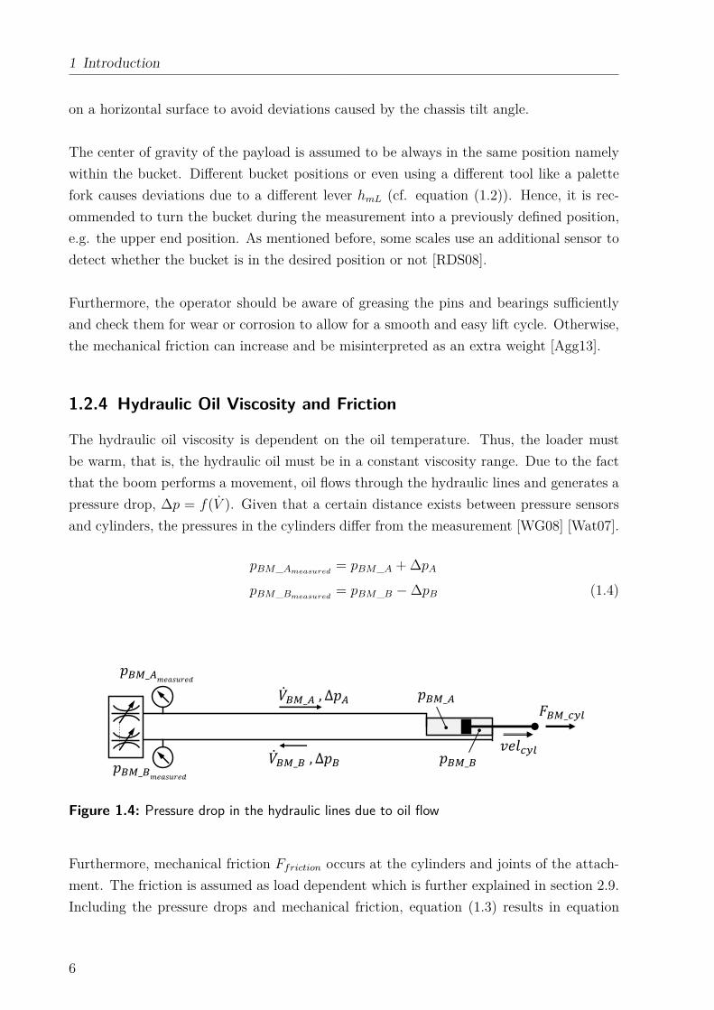
1.2.4 Hydraulic Oil Viscosity and Friction . . . . . . . . . . . . . . . . . 6
1.2.5 Calibration Procedure . . . . . . . . . . . . . . . . . . . . . . . . . 7
1.2.6 Current Research . . . . . . . . . . . . . . . . . . . . . . . . . . . . 9
1.2.7 Patents . . . . . . . . . . . . . . . . . . . . . . . . . . . . . . . . . 10
1.2.8 Potential for Improvement . . . . . . . . . . . . . . . . . . . . . . . 11
1.3 Objectives . . . . . . . . . . . . . . . . . . . . . . . . . . . . . . . . . . . . 13
1.4 Approach and Structure of this Thesis . . . . . . . . . . . . . . . . . . . . 13
2 Technical Basics 15
2.1 Kinematic Chain . . . . . . . . . . . . . . . . . . . . . . . . . . . . . . . . 15
2.2 Loader Kinematics . . . . . . . . . . . . . . . . . . . . . . . . . . . . . . . 17
2.2.1 Non Self-Leveling . . . . . . . . . . . . . . . . . . . . . . . . . . . . 17
2.2.2 Mechanical Self-Leveling . . . . . . . . . . . . . . . . . . . . . . . . 18
2.3 Coordinate Systems . . . . . . . . . . . . . . . . . . . . . . . . . . . . . . . 20
2.4 Coordinate Transformation . . . . . . . . . . . . . . . . . . . . . . . . . . . 21
2.5 Data Acquisition and Sensor Description . . . . . . . . . . . . . . . . . . . 23
2.6 Accelerations . . . . . . . . . . . . . . . . . . . . . . . . . . . . . . . . . . 24
2.6.1 Non-Inertial System K2 . . . . . . . . . . . . . . . . . . . . . . . . . 25
2.6.2 Non-Inertial System K3 . . . . . . . . . . . . . . . . . . . . . . . . . 26
2.6.3 Non-Inertial System K4 . . . . . . . . . . . . . . . . . . . . . . . . . 28
2.6.4 Acceleration at the Tractor . . . . . . . . . . . . . . . . . . . . . . . 28
V
Contents
2.6.5 Acceleration at the Front Loader . . . . . . . . . . . . . . . . . . . 30
2.6.5.1 Acceleration at the Boom . . . . . . . . . . . . . . . . . . 31
2.6.5.2 Acceleration at the Bucket . . . . . . . . . . . . . . . . . . 32
2.6.5.3 Acceleration at the Bucket, Measured with an IMU at the
Boom . . . . . . . . . . . . . . . . . . . . . . . . . . . . . 33
2.6.6 Gravity . . . . . . . . . . . . . . . . . . . . . . . . . . . . . . . . . 34
2.7 Mass and Center of Gravity . . . . . . . . . . . . . . . . . . . . . . . . . . 34
2.8 Moment of Inertia . . . . . . . . . . . . . . . . . . . . . . . . . . . . . . . . 36
2.9 Friction . . . . . . . . . . . . . . . . . . . . . . . . . . . . . . . . . . . . . 38
2.9.1 Seal Friction . . . . . . . . . . . . . . . . . . . . . . . . . . . . . . . 38
2.9.2 Lubrication . . . . . . . . . . . . . . . . . . . . . . . . . . . . . . . 39
2.9.3 Bearing Friction . . . . . . . . . . . . . . . . . . . . . . . . . . . . . 42
2.9.4 Friction Models . . . . . . . . . . . . . . . . . . . . . . . . . . . . . 42
2.9.4.1 Steady State Friction Model . . . . . . . . . . . . . . . . . 42
2.9.4.2 Dynamic Friction Model . . . . . . . . . . . . . . . . . . . 44
2.9.4.3 Pressure Based Model . . . . . . . . . . . . . . . . . . . . 45
3 Position Detection 47
3.1 Angle between Chassis and Boom . . . . . . . . . . . . . . . . . . . . . . . 47
3.2 Angle between Chassis and Bucket . . . . . . . . . . . . . . . . . . . . . . 49
3.3 Interchangeability and Sensor Configuration . . . . . . . . . . . . . . . . . 49
3.4 Continuous Angle Function . . . . . . . . . . . . . . . . . . . . . . . . . . 49
3.5 IMU Mounting Correction . . . . . . . . . . . . . . . . . . . . . . . . . . . 50
3.6 IMU Output Correction . . . . . . . . . . . . . . . . . . . . . . . . . . . . 51
3.7 Signal filtering . . . . . . . . . . . . . . . . . . . . . . . . . . . . . . . . . . 51
3.7.1 Observer . . . . . . . . . . . . . . . . . . . . . . . . . . . . . . . . . 53
3.7.1.1 Plant model . . . . . . . . . . . . . . . . . . . . . . . . . . 55
3.7.1.2 Observer model . . . . . . . . . . . . . . . . . . . . . . . . 55
3.7.1.3 Observer Gain . . . . . . . . . . . . . . . . . . . . . . . . 57
3.8 Cylinder Stroke to Angle Conversion . . . . . . . . . . . . . . . . . . . . . 59
3.9 Bucket Linkage Calculation . . . . . . . . . . . . . . . . . . . . . . . . . . 60
4 Weighing Function 63
4.1 Static Model . . . . . . . . . . . . . . . . . . . . . . . . . . . . . . . . . . . 64
4.1.1 Cylinder Forces . . . . . . . . . . . . . . . . . . . . . . . . . . . . . 65
4.1.2 Friction . . . . . . . . . . . . . . . . . . . . . . . . . . . . . . . . . 67
4.1.2.1 Approach of Friction Modeling . . . . . . . . . . . . . . . 67
4.1.2.2 Procedure of Friction Modeling . . . . . . . . . . . . . . . 68
VI
Contents
4.1.3 Torque Calculation . . . . . . . . . . . . . . . . . . . . . . . . . . . 75
4.1.3.1 Torque at the First Joint . . . . . . . . . . . . . . . . . . 75
4.1.3.2 Torque at the Second Joint . . . . . . . . . . . . . . . . . 76
4.2 Multi-Body Model of a Front Loader . . . . . . . . . . . . . . . . . . . . . 77
4.2.1 Differential Equations . . . . . . . . . . . . . . . . . . . . . . . . . 78
4.2.2 Parameters . . . . . . . . . . . . . . . . . . . . . . . . . . . . . . . 79
4.2.2.1 Accelerations . . . . . . . . . . . . . . . . . . . . . . . . . 80
4.2.2.2 Mass, Center of Gravity, and Inertia of a Part . . . . . . . 82
4.2.2.3 Considering the Parallel Axis Theorem . . . . . . . . . . . 83
4.3 Weighing Algorithm . . . . . . . . . . . . . . . . . . . . . . . . . . . . . . 84
4.3.1 Torque Equilibrium at the First Joint . . . . . . . . . . . . . . . . . 86
4.3.2 Torque Equilibrium at the Second Joint . . . . . . . . . . . . . . . 86
4.3.3 Payload Calculation . . . . . . . . . . . . . . . . . . . . . . . . . . 87
4.4 Roll and Pitch Angle of the Machine . . . . . . . . . . . . . . . . . . . . . 88
4.5 Implementation . . . . . . . . . . . . . . . . . . . . . . . . . . . . . . . . . 90
4.5.1 Payload . . . . . . . . . . . . . . . . . . . . . . . . . . . . . . . . . 91
4.5.2 Simplifications . . . . . . . . . . . . . . . . . . . . . . . . . . . . . . 91
4.5.2.1 Moments of Inertia . . . . . . . . . . . . . . . . . . . . . . 91
4.5.2.2 Oil Mass . . . . . . . . . . . . . . . . . . . . . . . . . . . . 91
4.5.2.3 Hoses . . . . . . . . . . . . . . . . . . . . . . . . . . . . . 92
4.5.2.4 Relative Movements . . . . . . . . . . . . . . . . . . . . . 92
4.5.2.5 Acceleration Sensor Position and Output . . . . . . . . . . 92
4.6 Optimized Model for Simple Parameter Identification . . . . . . . . . . . . 93
4.6.1 Reduced Multi-Body Model . . . . . . . . . . . . . . . . . . . . . . 94
4.6.2 Parameter Identification . . . . . . . . . . . . . . . . . . . . . . . . 96
4.6.3 Tractor Tilt Correction . . . . . . . . . . . . . . . . . . . . . . . . . 98
4.6.4 Torque Measurement . . . . . . . . . . . . . . . . . . . . . . . . . . 99
4.6.5 Deviation of the Total Loader Mass . . . . . . . . . . . . . . . . . . 100
4.6.6 Deviation Compared to the Full Multi-Body Model . . . . . . . . . 102
4.6.6.1 Merged Center of Gravity Position . . . . . . . . . . . . . 102
4.6.6.2 Estimated Moment of Inertia . . . . . . . . . . . . . . . . 104
5 Results 107
5.1 Benchmark for the Accuracy of the Test Results . . . . . . . . . . . . . . . 107
5.1.1 Accuracy Classes of Weighing Devices . . . . . . . . . . . . . . . . . 107
5.1.2 Required Accuracy of the Weighing System . . . . . . . . . . . . . 108
5.2 Dynamic Weighing vs. Common Systems . . . . . . . . . . . . . . . . . . . 109
5.3 Variation of the Payload’s Center of Gravity Position . . . . . . . . . . . . 112
VII
Contents
5.4 Friction Compensation . . . . . . . . . . . . . . . . . . . . . . . . . . . . . 116
5.5 Accelerations and Oscillations of the Front Loader . . . . . . . . . . . . . . 117
5.6 Repeatability . . . . . . . . . . . . . . . . . . . . . . . . . . . . . . . . . . 121
5.6.1 Working Cycles . . . . . . . . . . . . . . . . . . . . . . . . . . . . . 122
5.6.2 Continuous Payload Measurement . . . . . . . . . . . . . . . . . . . 125
6 Conclusion and Outlook 127
A Appendix A-1
A.1 Cylinder Center of Gravity Identification . . . . . . . . . . . . . . . . . . . A-1
A.2 Hardware . . . . . . . . . . . . . . . . . . . . . . . . . . . . . . . . . . . . A-3
A.3 Parameters . . . . . . . . . . . . . . . . . . . . . . . . . . . . . . . . . . . A-3
A.3.1 Mass, Center of Gravity, Inertia . . . . . . . . . . . . . . . . . . . . A-3
A.3.2 Dimensions . . . . . . . . . . . . . . . . . . . . . . . . . . . . . . . A-8
A.3.3 IMU Mounting Positions . . . . . . . . . . . . . . . . . . . . . . . . A-9
A.3.4 Cylinder Dimensions . . . . . . . . . . . . . . . . . . . . . . . . . . A-10
A.4 Fluid Film Thickness . . . . . . . . . . . . . . . . . . . . . . . . . . . . . . A-10
A.5 Machine Tilt Angle . . . . . . . . . . . . . . . . . . . . . . . . . . . . . . . A-11
A.6 Stiction - Settlement Effect . . . . . . . . . . . . . . . . . . . . . . . . . . . A-11
A.7 Simulating a Common System . . . . . . . . . . . . . . . . . . . . . . . . . A-16
A.8 Pressure Drop Identification . . . . . . . . . . . . . . . . . . . . . . . . . . A-17
A.9 Friction of Bearings . . . . . . . . . . . . . . . . . . . . . . . . . . . . . . . A-19
A.10 Bearing Friction versus Total Friction . . . . . . . . . . . . . . . . . . . . . A-20
A.11 Inertial Forces of Boom Actuators . . . . . . . . . . . . . . . . . . . . . . . A-21
A.12 Measurements . . . . . . . . . . . . . . . . . . . . . . . . . . . . . . . . . . A-23
Bibliography A-25
VIII
Indexes and Symbols
In general, all variables, indexes, and abbreviations are defined directly before they are
being used. Otherwise, they are defined in the following tables.
Table 1: Abbreviations and shortcuts
Abbr. Full form
2D two-dimensional
BM boom
BU bucket
COG, CoG center of gravity
config configuration
cf. compare
DOF degrees of freedom
DynWeiSys dynamic weighing system
deg degree
IMU inertial measurement unit
LTI linear time invariant
pos position
PTFE polytetrafluoroethylene
rec record
vs. versus
w with
w/o without
IX
Indexes and Symbols
Table 2: General indexes
Index Property
A piston side of the hydraulic actuator
B rod side of the hydraulic actuator
BM boom
BU bucket or tool carrier
CogSum overall center of gravity of several parts
cog center of gravity
cyl hydraulic cylinder or hydraulic actuator
g gravity
i counter
K coordinate system
L load
rod rod of the hydraulic actuator
P point in coordinate system or pendulum
piston piston of the hydraulic actuator
S sensor in coordinate system
S2 IMU mounted at the chassis
S3 IMU mounted at the boom
S4 IMU mounted at the bucket or tool carrier
sealPiston piston seal of the hydraulic actuator
sealRod rod seal of the hydraulic actuator
T tractor
trans translation
y y-component of a vector
X
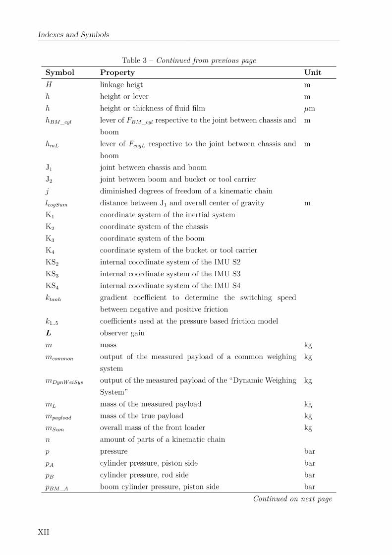
Table 3: Latin letters
Symbol Property Unit
A area m2
A system matrix of a LTI system
AA hydraulic effective area, piston side of a cylinder m2
AB hydraulic effective area, rod side of a cylinder m2
ABMBhydraulic effective area, rod side of the boom cylinder m2
Ar real area of sliding partner’s surface contact m2
Aδ1 steady state amplification of the disturbance δ1
a acceleration m/s2
~a acceleration vector m/s2
acyl acceleration of the hydraulic actuator movement m/s2
~aL acceleration at the payload m/s2
B viscous friction coefficient Ns/m
B control matrix of a LTI system
c amount of joints of a kinematic chain
C output matrix of a LTI system
D diameter m
D E.Lehr’s damping ratio
E Young’s modulus N/m2
e observer error
F force N
FBM_cyl force of the boom actuator N
FBU_cyl force of the bucket actuator N
FC Coulomb force N
FcogL weight force of the payload at its center of gravity N
Fcyl force of the hydraulic actuator N
Ffriction friction force N
Fg weight force N~Fjoint supporting force of the joint N
Fnormal normal force applied in the Hertz theory N
FS stiction force N
FsealP iston seal load used in the friction modeling N
FsealRod seal load used in the friction modeling N
f mobility of a kinematic chain
g gravity m/s2
Continued on next page
XI
Indexes and Symbols
Table 3 – Continued from previous page
Symbol Property Unit
H linkage heigt m
h height or lever m
h height or thickness of fluid film µm
hBM_cyl lever of FBM_cyl respective to the joint between chassis and
boom
m
hmL lever of FcogL respective to the joint between chassis and
boom
m
J1 joint between chassis and boom
J2 joint between boom and bucket or tool carrier
j diminished degrees of freedom of a kinematic chain
lcogSum distance between J1 and overall center of gravity m
K1 coordinate system of the inertial system
K2 coordinate system of the chassis
K3 coordinate system of the boom
K4 coordinate system of the bucket or tool carrier
KS2 internal coordinate system of the IMU S2
KS3 internal coordinate system of the IMU S3
KS4 internal coordinate system of the IMU S4
ktanh gradient coefficient to determine the switching speed
between negative and positive friction
k1..5 coefficients used at the pressure based friction model
L observer gain
m mass kg
mcommon output of the measured payload of a common weighing
system
kg
mDynW eiSys output of the measured payload of the “Dynamic Weighing
System”
kg
mL mass of the measured payload kg
mpayload mass of the true payload kg
mSum overall mass of the front loader kg
n amount of parts of a kinematic chain
p pressure bar
pA cylinder pressure, piston side bar
pB cylinder pressure, rod side bar
pBM_A boom cylinder pressure, piston side bar
Continued on next page
XII
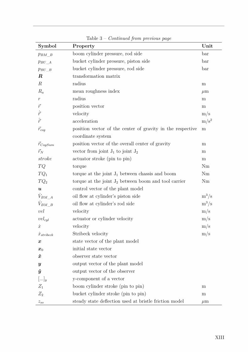
Table 3 – Continued from previous page
Symbol Property Unit
pBM_B boom cylinder pressure, rod side bar
pBU_A bucket cylinder pressure, piston side bar
pBU_B bucket cylinder pressure, rod side bar
R transformation matrix
R radius m
Ra mean roughness index µm
r radius m
~r position vector m
~r velocity m/s
~r acceleration m/s2
~rcog position vector of the center of gravity in the respective
coordinate system
m
~rCogSum position vector of the overall center of gravity m
~rN vector from joint J1 to joint J2 m
stroke actuator stroke (pin to pin) m
TQ torque Nm
TQ1 torque at the joint J1 between chassis and boom Nm
TQ2 torque at the joint J2 between boom and tool carrier Nm
u control vector of the plant model
VBM_A oil flow at cylinder’s piston side m3/s
VBM_B oil flow at cylinder’s rod side m3/s
vel velocity m/s
velcyl actuator or cylinder velocity m/s
x velocity m/s
xstribeck Stribeck velocity m/s
x state vector of the plant model
x0 initial state vector
x observer state vector
y output vector of the plant model
y output vector of the observer
[...]y y-component of a vector
Z1 boom cylinder stroke (pin to pin) m
Z2 bucket cylinder stroke (pin to pin) m
zss steady state deflection used at bristle friction model µm
XIII
Indexes and Symbols
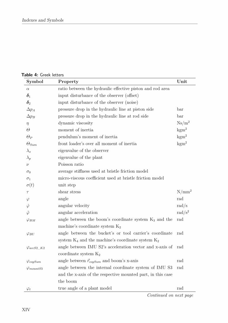
Table 4: Greek letters
Symbol Property Unit
α ratio between the hydraulic effective piston and rod area
δ1 input disturbance of the observer (offset)
δ2 input disturbance of the observer (noise)
∆pA pressure drop in the hydraulic line at piston side bar
∆pB pressure drop in the hydraulic line at rod side bar
η dynamic viscosity Ns/m2
Θ moment of inertia kgm2
ΘP pendulum’s moment of inertia kgm2
ΘSum front loader’s over all moment of inertia kgm2
λo eigenvalue of the observer
λp eigenvalue of the plant
ν Poisson ratio
σ0 average stiffness used at bristle friction model
σ1 micro-viscous coefficient used at bristle friction model
σ(t) unit step
τ shear stress N/mm2
ϕ angle rad
ϕ angular velocity rad/s
ϕ angular acceleration rad/s2
ϕBM angle between the boom’s coordinate system K3 and the
machine’s coordinate system K2
rad
ϕBU angle between the bucket’s or tool carrier’s coordinate
system K4 and the machine’s coordinate system K2
rad
ϕaccS2_K2 angle between IMU S2’s acceleration vector and x-axis of
coordinate system K2
rad
ϕcogSum angle between ~rcogSum and boom’s x-axis rad
ϕmountS3 angle between the internal coordinate system of IMU S3
and the x-axis of the respective mounted part, in this case
the boom
rad
ϕt true angle of a plant model rad
Continued on next page
XIV
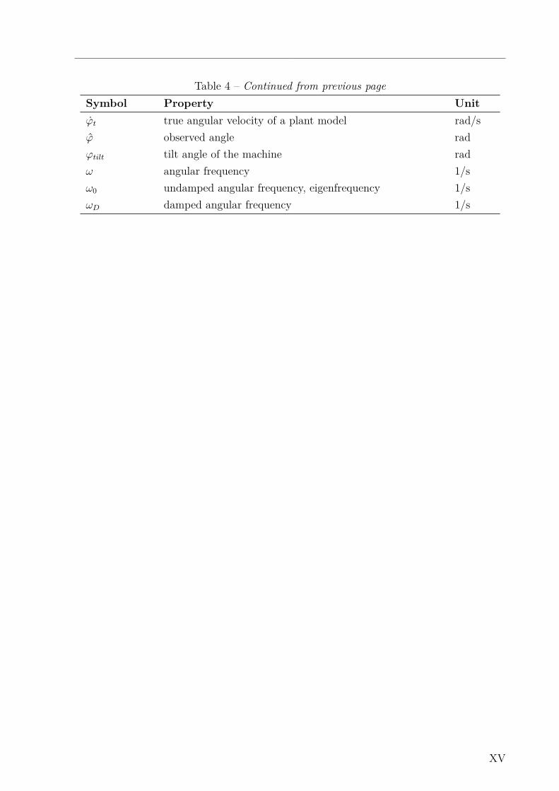
Table 4 – Continued from previous page
Symbol Property Unit
ϕt true angular velocity of a plant model rad/s
ϕ observed angle rad
ϕtilt tilt angle of the machine rad
ω angular frequency 1/s
ω0 undamped angular frequency, eigenfrequency 1/s
ωD damped angular frequency 1/s
XV

Abstract
In many industrial applications it is a benefit to measure payload while handling it. For
instance, the cost of material loaded on a dump truck in a quarry is generally priced by
its weight. In this case, the truck has to pass a stationary scale twice to identify its pay-
load, before and after loading. Measuring weight of the material instantly while loading
the truck, increases the efficiency of the process and makes a stationary scale redundant.
Moreover, it is necessary to measure weight, for example, to efficiently loading a trailer to
its maximum capacity without exceeding the gross load weight. Another example, where a
payload measurement is useful, is when filling a biogas plant with a defined mass of organic
material. Furthermore, the productivity and efficiency of a dairy farm can be increased by
measuring the weight of cattle food in order to supply the right amount of cattle food di-
rectly while filling the feeders. Usually, the payload is being handled by a common tractor
front loader, wheel loader, or telescopic loader. Hence, it is reasonable to use the loader
itself as a scale.
Currently, a variety of loader scales are available on the market. The functionality of
most mobile scales is largely identical. The accuracy of the payload measurement is ac-
ceptable as long as the measurement is taken at a previous specified loader attachment
position during a defined boom up movement. Throughout the measurement process, the
machine must not bounce or oscillate and only smooth movements are allowed. To achieve
a high accuracy, the center of gravity of the payload must be in a previously defined posi-
tion. Generally, this is obtained by moving the bucket cylinders to the upper end stroke
position and assuming the center of gravity of the payload to be always in the bucket at
the same position. This applies to a bucket that is completely filled with bulk material of
a constant density such as sand or gravel. If the bucket is only partly filled, the center of
gravity position of the payload will vary. Furthermore, with different tools attached, for
instance a palette fork or a bale clamp, the center of gravity position of the payload will
change. This causes deviations in the payload measurement.
Analyzing these scales revealed that there is a need for an integrated and flexible technical
solution for dynamic and continuous weighing of the payload during the operator’s work
process. This solution needs to be independent of the center of gravity position of the
payload which in turn allows the use of any attached tool such as buckets, palette forks,
or bale clamps. The payload measurement must be independent of the position and move-
ments of the attachment, as well as independent of the position and its movements of the
machine. The calibration process of the scale must be easy to perform and adaptable to
XVII
Abstract
structure changes, such as mounting an additional valve to the boom.
To meet these demands, this thesis deals with the research and development of a mo-
bile loader scale. The underlying theory is concerned with the combination of two models;
a static model which deals with the dimensions and actuator forces of the loader; and a
multi-body model which deals with accelerations. The static model transfers measured ac-
tuator forces into torques at the joints of an open planar kinematic chain which represents
the boom and bucket with their joints. The multi-body model transfers actual acceler-
ations of loader movements into forces. These forces in connection with their respective
levers, generate torques at the joints as well. These torques are set in relation to each
other. Hence, the multi-body model considers a loader without payload. The torques from
the static model and the torques from the multi-body model differ from each other so that
a calculation of the payload is possible. Measuring accelerations in all axis and providing
them to the multi-body model allows to compensate oscillations of the loader movements.
Also, tilting of the machine is compensated in this way.
The independence of the measurement of the center of gravity position of the payload
is realized by considering the torques at both joints of the open planar kinematic chain
which implies the use of the boom and bucket actuator forces. Thus, any tool can be
attached without an additional calibration, even a tool with an additional moving arm
such as a crane or excavator attachment.
Due to the cylinder and joint friction, the measured actuator forces deviate from the
forces which are needed to lift the payload. For instance, the measured actuator force for
the same payload will be higher for a boom up movement than at standstill and lower
for boom down movement. This disturbs the payload measurement. Hence, friction is
estimated with a friction model to counteract these effects.
Usually, scales are categorized and benchmarked by their accuracy. In this case, the
accuracy of the payload measurement strongly relies on the accuracy of the models. It
is very time consuming to build an accurate multi-body model and identifying all of its
parameters. Either the model and its parameters are derived from 3D-CAD data or a real
loader is taken apart and each parameter is measured in tests as done in this thesis. A
model derived from 3D-CAD data underlies manufacturing tolerances and does not con-
sider changes made to the loader afterwards, such as adding an additional valve to the
boom. Deriving the multi-body model by tests requires a lot of effort but is very accurate
for one loader. Due to variance in manufacturing outcomes, test results cannot be trans-
fered but have to be conducted for every single machine. This led to the development of
XVIII
a reduced multi-body model that obtains its parameters partly from 3D-CAD data and
partly from a short calibration procedure. In this case, the reduced multi-body model
is self-adjusting and covers all manufacturing tolerances. For later changes to the front
loader the calibration procedure can easily be redone.
In order to measure payload continuously at any time, the static model and the multi-
body model require a continuous position detection of the loader relative to the machine.
To obtain a reliable measurement system, which is also easy to retrofit on existing load-
ers, the position detection is implemented with three inertial measurement units (IMUs)
connected to the chassis, boom, tool carrier, or bucket. IMUs consist only of non-moving
parts and can be mounted anywhere in a protected position.
Finally, this thesis presents the implementation and testing of the dynamic and contin-
uous mobile scale on an agricultural tractor front loader that measures independently of
the center of gravity position of the payload. Further analyses reveal that it is possible
to measure payload during the working process with a deviation of 1% of the maximum
loading capacity.
XIX


Kurzfassung
In vielen industriellen Bereichen ist es vorteilhaft das Gewicht einer Nutzlast während der
Abfertigung oder dem Transport zu messen. In einer Mine oder einem Steinbruch werden
zum Beispiel die Materialkosten für eine Lastwagenladung für gewöhnlich durch das Ge-
wicht ermittelt. Um das Gewicht der Ladung zu bestimmen, muss der Lastwagen zweimal
eine stationäre Waage passieren, vor und nach dem Laden. Wenn man das Gewicht konti-
nuierlich beim Beladen misst, kann man die Effizienz des gesamten Prozesses steigern und
eine stationäre Waage ist überflüssig.
Eine direkte Gewichtsmessung erweist sich auch dann als sinnvoll, wenn man einen An-
hänger möglichst effizient beladen möchte ohne dabei das maximale Bruttolastgewicht zu
überschreiten. Ein weiteres Beispiel für die Vorteile einer direkten Gewichtsmessung ist das
Beschicken einer Biogasanlage mit einer definierten Masse an organischem Material. Eine
Steigerung der Produktivität und Effizienz kann auch in einem Viehbetrieb erlangt werden,
indem man die richtige Menge an Nahrung direkt während der Befüllung der Futteranlagen
abwiegt, anstatt das Gewicht davor auf einer stationären Waage zu wiegen oder einfach nur
zu schätzen. In der Regel werden Lasten mit einem Traktor Frontlader, Radlader oder Te-
leskoplader transportiert. Daher ist es naheliegend den Lader selbst als Waage einzusetzen.
Derzeit sind mehrere verschiedene mobile Lader-Waagen auf dem Markt erhältlich. Die
meisten Waagen basieren auf dem selben Funktionsprinzip. Die Genauigkeit dieser Waa-
gen ist nur gegeben, wenn die Messung in einer vorher definierten Schwingenposition und
bei einer bestimmten Zylinderverfahrgeschwindigkeit erfolgt. Während des Messvorgangs
darf sich die Maschine nicht ruckartig bewegen oder schwingen. Es sind nur sanfte, konti-
nuierliche Bewegungen erlaubt.
Um eine hohe Genauigkeit der Gewichtsmessung zu erreichen, muss sich der Schwerpunkt
der Ladung in einer vorher definierten Position befinden. Im Allgemeinen wird dies erreicht
indem die Schaufelzylinder in die obere Endposition gefahren werden. Außerdem gilt die
Annahme, dass der Ladungsschwerpunkt sich immer innerhalb der Schaufel und an der
gleichen Position befindet. Dies gilt nur dann, wenn die Schaufel vollständig mit Schüttgut
von konstanter Dichte gefüllt ist, wie zum Beispiel Sand oder Kies. Die Schwerpunktlage
variiert jedoch, wenn die Schaufel nur teilweise gefüllt wird. Wird die Schaufel gegen andere
Werkzeuge ausgetauscht, wie zum Beispiel eine Palettengabel oder eine Heuballenzange,
so ändert sich die Schwerpunktlage bei jeder neuen Ladungsaufnahme und verursacht Ab-
weichungen in der Gewichtsmessung.
XXI

Kurzfassung
Die Analyse der bestehenden mobilen Lader-Waagen zeigt, dass der Bedarf einer integrier-
ten und flexiblen technischen Lösung einer mobilen Lader-Waage besteht, die kontinuierlich
und dynamisch während des Arbeitsvorgangs wiegen kann. Diese Waage muss das Gewicht
unabhängig von der Schwerpunktlage der Ladung messen, was den Einsatz beliebiger Werk-
zeuge, wie zum Beispiel verschiedener Schaufeln, einer Palettengabel oder einer Heubal-
lenzange ermöglicht. Die Gewichtsmessung muss unabhängig von der Schaufel-, Arm- und
Maschinenposition oder Bewegung erfolgen. Außerdem muss der Kalibrierungsprozess der
Waage einfach durchzuführen und anpassbar sein, um schnell auf Änderungen reagieren
zu können, wie zum Beispiel der Montage eines zusätzlichen Ventils auf der Laderschwinge.
Um diesen Anforderungen gerecht zu werden, beschäftigt sich diese Arbeit mit der For-
schung und Entwicklung einer mobilen Lader-Waage. Die zugrunde liegende Theorie kom-
biniert zwei Modelle: Ein statisches Modell, welches die Dimensionen des Laders und die
Aktuatorkräfte berücksichtigt und ein Mehrkörpermodell, welches verwendet wird um Be-
schleunigungen zu verarbeiten. Das statische Modell wandelt gemessene Aktuatorkräfte
in Drehmomente an den Gelenken einer offenen, ebenen, kinematischen Kette um, welche
die Schwinge und Schaufel mit den jeweiligen Gelenken darstellt. Das Mehrkörpermodell
überträgt die aus den Bewegungen des Laders resultierenden Beschleunigungen in Kräfte.
Diese Kräfte erzeugen, mit ihren jeweiligen Hebeln, ebenso Drehmomente an den Gelen-
ken. Anschließend werden die Drehmomente aus den verschiedenen Modellen in Relation
zueinander gesetzt. Die Drehmomente des Mehrkörpermodells, das die Ladung nicht be-
rücksichtigt, und die Drehmomente des statischen Modells, das mit gemessenen Aktuator-
kräften gespeist wird, unterscheiden sich. Aus diesem Unterschied kann nun das Gewicht
der Ladung bestimmt werden. Die Schwingungen und Bewegungen des Laders werden kom-
pensiert, da das Mehrkörpermodell mit direkt gemessenen mehrachsigen Beschleunigungen
gespeist wird. Ebenso werden Neigungen der Maschine ausgeglichen, die zum Beispiel bei
Arbeiten am Hang entstehen.
Durch die Berücksichtigung der Aktuatorkräfte von Schwinge und Schaufel können die
Drehmomente an beiden Gelenken der offenen ebenen kinematischen Kette bestimmt wer-
den, wodurch die Gewichtsbestimmung unabhängig der Ladungs-Schwerpunktslage ermög-
licht wird. Somit kann jedes Werkzeug oder Anbaugerät ohne zusätzliche Kalibrierung
eingesetzt werden. Darüber hinaus kann ein Anbaugerät mit einem zusätzlichen bewegli-
chen Arm eingesetzt werden, ähnlich einem Kran oder einer Grabausrüstung eines Baggers.
Aufgrund der Zylinder- und Gelenkreibung weichen die gemessenen Aktuatorkräfte von
den Aktuatorkräften ab, die erforderlich sind die Ladung in Position zu halten. Für die
XXII

gleiche Ladung ist, beispielsweise, die gemessene Aktuatorkraft während der Schwingen-
aufwärtsbewegung höher und während der Abwärtsbewegung niedriger als bei Stillstand.
Dies führt zu Abweichungen in der Gewichtbestimmung. Um diesem Effekt entgegenzuwir-
ken wird die Reibung mithilfe eines Reibmodells abgeschätzt und in der Gewichtsmessung
berücksichtigt.
Waagen werden unter anderem anhand ihrer Messgenauigkeit kategorisiert und bewer-
tet. Die Genauigkeit der Gewichtsmessung ist stark abhängig von den Genauigkeiten der
Modelle. Es ist sehr zeitaufwendig alle Parameter zu identifizieren, um ein genaues Mehr-
körpermodell zu erstellen. Entweder werden das Modell und dessen Parameter von 3D-
CAD-Daten abgeleitet oder ein echter Lader wird demontiert und zerlegt und die Parame-
ter werden durch verschiedene Tests bestimmt, wie es in dieser Arbeit erfolgte. Wird ein
Modell aus 3D-CAD-Daten abgeleitet, bestehen infolge von Fertigungstoleranzen Abwei-
chungen zur Realität. Außerdem werden keine Änderungen berücksichtigt, die nachträg-
lich am Lader gemacht wurden, wie zum Beispiel das Anbringen eines zusätzlichen Ventils
an der Schwinge. Das Identifizieren der Mehrkörpermodellparameter durch Tests ist sehr
präzise für einen einzelnen Lader, bedeutet jedoch einen erheblichen Arbeitsaufwand. Auf-
grund der Fertigungstoleranzen können die Parameter nicht übertragen werden, sodass die
Identifikation für jeden einzelnen Lader erneut durchgeführt werden muss. Auf der Suche
nach einem einfacheren und weniger arbeitsaufwendigen Verfahren wurde ein reduziertes
Mehrkörpermodell entwickelt, dessen Parameter teilweise von 3D-CAD-Daten abgeleitet
werden und teilweise durch ein kurzes Kalibrierverfahren identifiziert werden. Dadurch
wird das reduzierte Mehrkörpermodell für jeden Lader automatisch angepasst und deckt
alle Fertigungstoleranzen ab. Für spätere Änderungen am Lader kann die Kalibrierung
leicht wiederholt werden.
Für das statische Modell und das Mehrkörpermodell ist eine kontinuierliche Positions-
erfassung der Schwinge und Schaufel zur Maschine nötig, um das Gewicht der Ladung
kontinuierlich messen zu können. Ein zuverlässiges Messsystem, das auch einfach an beste-
henden Ladern nachgerüstet werden kann, wird mit drei inertialen Messeinheiten (Inertial
Measurement Unit, IMU ) umgesetzt. Die IMUs sind jeweils an der Maschine, der Schwinge
und der Schaufel beziehungsweise dem Geräteträger angebracht. Der Vorteil besteht dar-
in, dass IMUs keine beweglichen Teile beinhalten und an einer beliebigen, vor Zerstörung
geschützten, Position angebracht werden können.
Abschließend wurde die mobile Waage als Prototyp an einem Traktor Frontlader installiert.
Weitere Analysen zeigen, dass man mit dieser Waage das Gewicht kontinuierlich während
des Arbeitsablaufes messen kann. Dies erfolgt mit einer Abweichung von 1% der maximalen
Ladekapazität.
XXIII

1 Introduction
1.1 Motivation
For many loader applications it is a benefit to measure the payload directly while handling
it. For instance, the costs of material loaded on a dump truck in a quarry is generally
priced by its weight. In this case, the truck has to pass a stationary scale twice to identify
its payload, before and after loading. Measuring the weight of the material instantly while
loading the truck would increase the efficiency of the process and a stationary scale would
be redundant. Also, in many farming tasks it is necessary to measure weight, for example,
to efficiently load a trailer with goods to its maximum capacity without exceeding the gross
load weight or filling a bio-gas plant with a defined mass of organic material. Generally,
a common tractor front loader, wheel loader, or telescopic loader handles the payload.
Hence, it is obvious to use the loader itself as a scale.
Using the loader as a scale offers new possibilities for documentation, billing and mon-
itoring the transfer of goods, such as hay bales, palettes, etc. For example, it allows
contractors to measure the work in the quantity of the handled payload and change their
hourly payment into a merit pay, according to the results or effort or wear of the loader. In
addition, by measuring the payload continuously, also discontinuous media, such as seeds,
at varying density could be monitored. For instance, precision farming applications de-
mand tracing the spread of seeds or fertilizer on the fields to optimize the yield according
to the sowing [Tre02]. Combining a positioning system, like a global navigation satellite
system (GNSS), with a continuous payload measurement allows to calculate and to control
the mass flow mpayload of the seeds or fertilizer at any position on the field. Other farming
applications are described by [Loa14a] and [Loa14b] where farmers increase their produc-
tivity by weighing the feed for dairy cows with a mobile front loader scale. It allows them
to supply the exact amount of food to promote the optimum levels of milk productions
and to monitor the weight totals of food accurately.
[Vei13] explains that measuring the payload with the loader directly reduces fuel con-
sumption in a mine due to the elimination of under loads and waiting times at the loading
site when the truck was overloaded.
Currently, a variety of loader scales is available on the market. The functionality for
most mobile scales is largely the same. The accuracy of the payload measurement is good
1
1 Introduction
as long as specific boundary conditions are fulfilled (cf. section 1.2.3). Studying those
scales revealed that there is a need for an integrated and flexible technical solution for
dynamic and continuous weighing of the payload during the operator’s work process. This
solution needs to be independent of:
• the center of gravity position of the payload
• the attached tool (e.g. bucket, palette fork, etc.)
• the loader position and its movements
• the vehicle position and its movements.
In order to achieve these goals, this thesis deals with the research and development of a
new kind of mobile loader scale.
1.2 State of the Art of Mobile Scales
Currently, several wheel loader and front loader scales are available on the market with an
achieved accuracy of class four which corresponds to an ordinary scale [PFR14] [DIN92] (cf.
section 5.1.1 for more detailed information on accuracy classes). The technical functionality
is generally the same. Differences mostly occur within further processing capacities. This
chapter mainly focuses on the technical realization of available scales and their capabilities.
1.2.1 General Functioning
There are several ways to measure the payload attached to the movable boom of a mobile
machine, for example, a front loader, wheel loader, telescopic loader, or excavator. Some
mobile scales for telescopic loaders measure the bending strain of the long boom to deter-
mine the payload. Therefore, strain gauges are applied directly to the boom or mounted
by a load cell [Pro12a] [BAR13] [Fli11b]. This kind of scale is not further discussed in this
thesis. Most loader scales use the cylinder forces to determine the payload which is usually
calculated by measured pressures at the piston and rod sides of the boom cylinders.
2
1.2 State of the Art of Mobile Scales
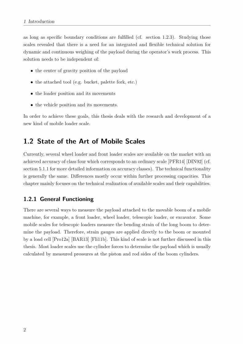
boom (BM)
bucket (BU)
payload
chassis
vehicle, loader
attachment, front loader
joint J1
joint J2
boom cylinder bucket cylinder
center of gravityof the payload
Figure 1.1: Loader description
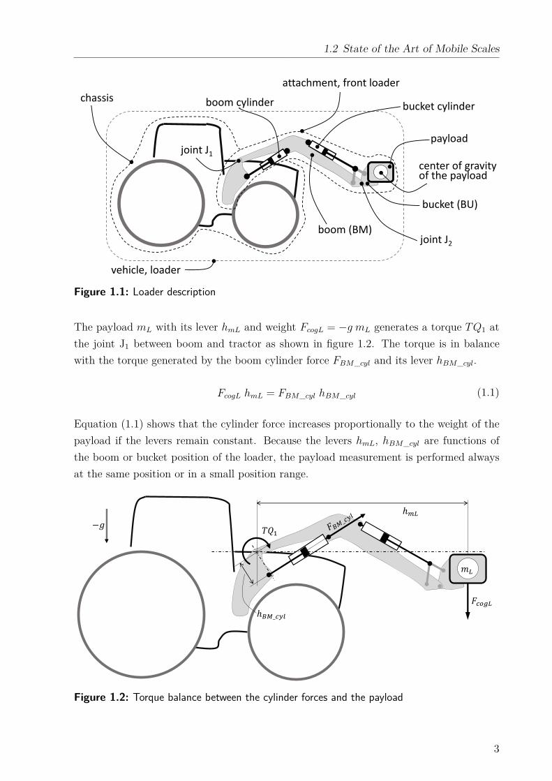
The payload mL with its lever hmL and weight FcogL = −g mL generates a torque TQ1 at
the joint J1 between boom and tractor as shown in figure 1.2. The torque is in balance
with the torque generated by the boom cylinder force FBM_cyl and its lever hBM_cyl.
FcogL hmL = FBM_cyl hBM_cyl (1.1)
Equation (1.1) shows that the cylinder force increases proportionally to the weight of the
payload if the levers remain constant. Because the levers hmL, hBM_cyl are functions of
the boom or bucket position of the loader, the payload measurement is performed always
at the same position or in a small position range.
� �
ℎ
ℎ��_
−�
Figure 1.2: Torque balance between the cylinder forces and the payload
3
1 Introduction
Finally, equation (1.2) determines the payload based on the cylinder force.
mL =
(
hBM_cyl
−g hmL
)
FBM_cyl = kFBM_cyl (1.2)
The constant parameter k is in principle identified by a previous two point calibration with
two different known weights mL1 and mL2, as described in chapter 1.2.5.
1.2.2 Setup and Components
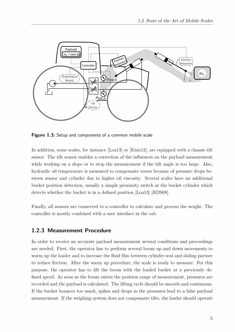
To measure the payload, the loader is equipped with several sensors. The boom cylinder
pressures pBM_A and pBM_B are measured with sensors located in the hydraulic lines
between cylinder and valve, as shown in figure 1.3. The cylinder forces can be calculated
with the knowledge of the areas of piston and rod sides. However, due to the previous
load calibration (cf. section 1.2.5) this is not necessary. It is sufficient to obtain a scaled
cylinder force FBM_cylscaled, from equation (1.3), which is set into relation with the payload
and can be calculated with the cylinder ratio between piston area AA and rod area AB
(ram-ratio, α =AA
AB
), mostly in the range of 1.25 to 1.34 [RDS08] [WG08]. The friction is
not yet considered.
FBM_cylscaled=
FBM_cyl
ABMB
= pBM_Aα − pBM_B (1.3)
Furthermore, the boom position is needed. Since the payload measurement is always per-
formed at the same position, it is sufficient to determine, using a proximity switch, if the
boom is at the desired measuring position.
In addition, friction has to be considered because the front loader experiences friction
in cylinders and bearings. Hence, it is recommended to perform the payload measurement
within a defined speed range during a front loader up-movement [Fli11a]. The movement
causes sliding friction which is lower than stiction. Thus, the average of a continuous
pressure measurement is taken in a small boom position range. The start and end of this
position range is often taken with two proximity switches. Moreover, by detecting start
and end-time, it is possible to calculate the average speed of the front loader movement
[Pro12b]. Some scales, for instance [Loa13], use continuous position detection with angle
or stroke sensors instead of proximity switches.
4
1.2 State of the Art of Mobile Scales
��_��_�
Tilt
Sensor
Payload
= xxxx kg
Temperature
Sensor
Position
DetectionController
Figure 1.3: Setup and components of a common mobile scale
In addition, some scales, for instance [Loa13] or [Käm12], are equipped with a chassis tilt
sensor. The tilt sensor enables a correction of the influences on the payload measurement
while working on a slope or to stop the measurement if the tilt angle is too large. Also,
hydraulic oil temperature is measured to compensate errors because of pressure drops be-
tween sensor and cylinder due to higher oil viscosity. Several scales have an additional
bucket position detection, usually a simple proximity switch at the bucket cylinder which
detects whether the bucket is in a defined position [Loa13] [RDS08].
Finally, all sensors are connected to a controller to calculate and process the weight. The
controller is mostly combined with a user interface in the cab.
1.2.3 Measurement Procedure
In order to receive an accurate payload measurement several conditions and proceedings
are needed. First, the operator has to perform several boom up and down movements to
warm up the loader and to increase the fluid film between cylinder seal and sliding partner
to reduce friction. After the warm up procedure, the scale is ready to measure. For this
purpose, the operator has to lift the boom with the loaded bucket at a previously de-
fined speed. As soon as the boom enters the position range of measurement, pressures are
recorded and the payload is calculated. The lifting cycle should be smooth and continuous.
If the bucket bounces too much, spikes and drops in the pressures lead to a false payload
measurement. If the weighing system does not compensate tilts, the loader should operate
5
1 Introduction
on a horizontal surface to avoid deviations caused by the chassis tilt angle.
The center of gravity of the payload is assumed to be always in the same position namely
within the bucket. Different bucket positions or even using a different tool like a palette
fork causes deviations due to a different lever hmL (cf. equation (1.2)). Hence, it is rec-
ommended to turn the bucket during the measurement into a previously defined position,
e.g. the upper end position. As mentioned before, some scales use an additional sensor to
detect whether the bucket is in the desired position or not [RDS08].
Furthermore, the operator should be aware of greasing the pins and bearings sufficiently
and check them for wear or corrosion to allow for a smooth and easy lift cycle. Otherwise,
the mechanical friction can increase and be misinterpreted as an extra weight [Agg13].
1.2.4 Hydraulic Oil Viscosity and Friction
The hydraulic oil viscosity is dependent on the oil temperature. Thus, the loader must
be warm, that is, the hydraulic oil must be in a constant viscosity range. Due to the fact
that the boom performs a movement, oil flows through the hydraulic lines and generates a
pressure drop, ∆p = f(V ). Given that a certain distance exists between pressure sensors
and cylinders, the pressures in the cylinders differ from the measurement [WG08] [Wat07].
pBM_Ameasured= pBM_A + ∆pA
pBM_Bmeasured= pBM_B − ∆pB (1.4)
��_� �
��_ �
����_���_
���_� , ∆ � ���_ , ∆ ���_
Figure 1.4: Pressure drop in the hydraulic lines due to oil flow
Furthermore, mechanical friction Ffriction occurs at the cylinders and joints of the attach-
ment. The friction is assumed as load dependent which is further explained in section 2.9.
Including the pressure drops and mechanical friction, equation (1.3) results in equation
6
1.2 State of the Art of Mobile Scales
(1.5) which is proportional to the payload mL.
mL ∼ FBM_cylmeasured
ABM_B
= pBM_Aα − pBM_B + (∆pAα + ∆pB) +Ffriction
ABM_B
(1.5)
Due to the bracket term which considers the pressure drops because of the oil flow, the
measured cylinder force appears higher than it really is and falsifies the payload measure-
ment. The challenge is to define this bracket term for different cylinder speeds at defined
oil temperatures by previous calibration procedures and subtract it from the measured
cylinder force to correct the payload measurement.
1.2.5 Calibration Procedure
To set the cylinder forces FBM_cyl or FBM_cylscaledin relation to the payload, the weigh-
ing system has to be calibrated. Before the operator starts the calibration, the hydraulic
oil has to be warmed up to normal working conditions to receive a constant oil viscosity.
Also, several lifting cycles have to be performed to lubricate the joints and the cylinder rod.
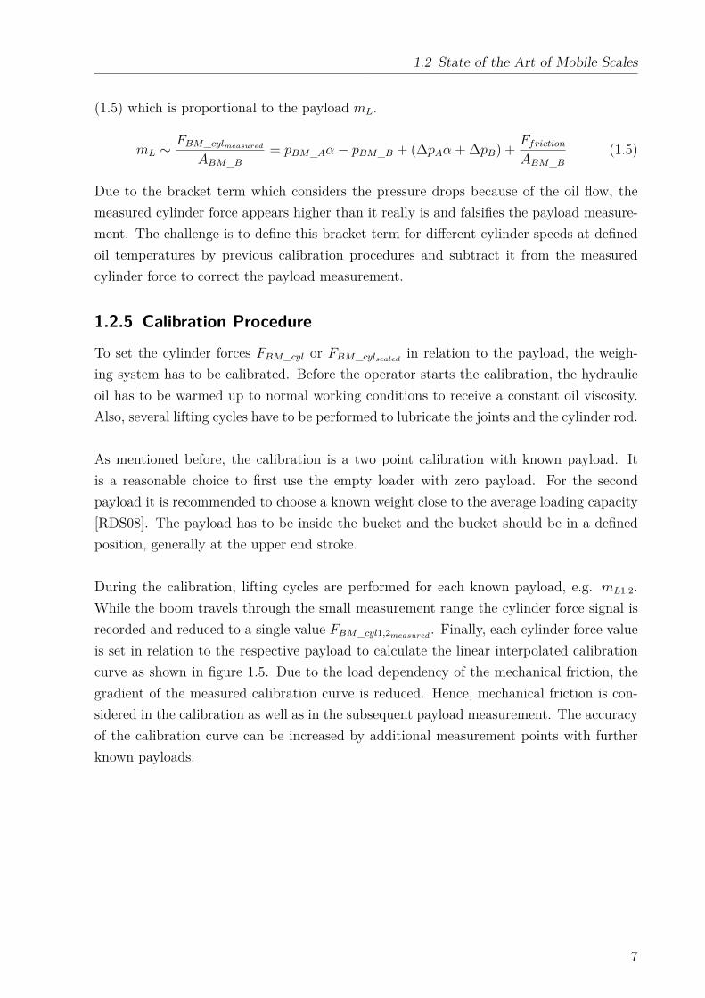
As mentioned before, the calibration is a two point calibration with known payload. It
is a reasonable choice to first use the empty loader with zero payload. For the second
payload it is recommended to choose a known weight close to the average loading capacity
[RDS08]. The payload has to be inside the bucket and the bucket should be in a defined
position, generally at the upper end stroke.
During the calibration, lifting cycles are performed for each known payload, e.g. mL1,2.
While the boom travels through the small measurement range the cylinder force signal is
recorded and reduced to a single value FBM_cyl1,2measured. Finally, each cylinder force value
is set in relation to the respective payload to calculate the linear interpolated calibration
curve as shown in figure 1.5. Due to the load dependency of the mechanical friction, the
gradient of the measured calibration curve is reduced. Hence, mechanical friction is con-
sidered in the calibration as well as in the subsequent payload measurement. The accuracy
of the calibration curve can be increased by additional measurement points with further
known payloads.
7
1 Introduction
pa
ylo
ad
cylinder force ���_���_ � � � ���_ � � �
� �� ��
Figure 1.5: Two point calibration
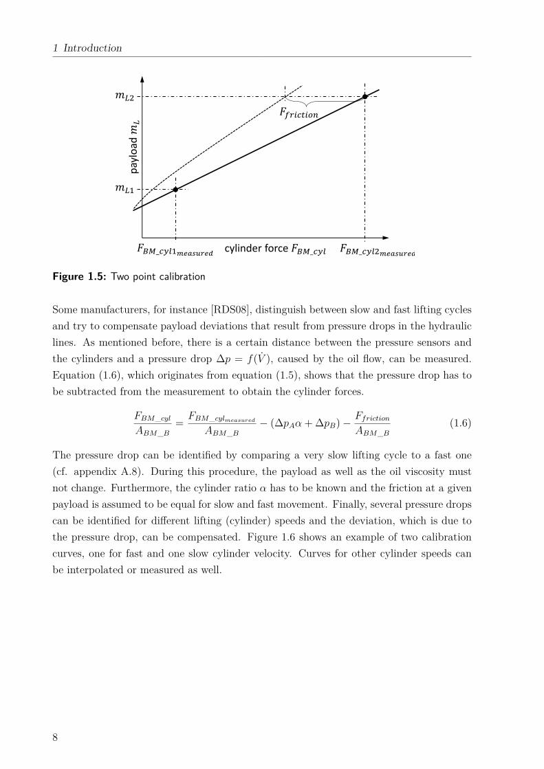
Some manufacturers, for instance [RDS08], distinguish between slow and fast lifting cycles
and try to compensate payload deviations that result from pressure drops in the hydraulic
lines. As mentioned before, there is a certain distance between the pressure sensors and
the cylinders and a pressure drop ∆p = f(V ), caused by the oil flow, can be measured.
Equation (1.6), which originates from equation (1.5), shows that the pressure drop has to
be subtracted from the measurement to obtain the cylinder forces.
FBM_cyl
ABM_B
=FBM_cylmeasured
ABM_B
− (∆pAα + ∆pB) − Ffriction
ABM_B
(1.6)
The pressure drop can be identified by comparing a very slow lifting cycle to a fast one
(cf. appendix A.8). During this procedure, the payload as well as the oil viscosity must
not change. Furthermore, the cylinder ratio α has to be known and the friction at a given
payload is assumed to be equal for slow and fast movement. Finally, several pressure drops
can be identified for different lifting (cylinder) speeds and the deviation, which is due to
the pressure drop, can be compensated. Figure 1.6 shows an example of two calibration
curves, one for fast and one slow cylinder velocity. Curves for other cylinder speeds can
be interpolated or measured as well.
8
1.2 State of the Art of Mobile Scales
pa
ylo
ad
measured
cylinder force���_ _slow ���_ _fast
�∆ + ∆ �
Figure 1.6: Pressure drop compensation
1.2.6 Current Research
This chapter deals with the current research of mobile scales and their different approaches
to increase the performance of mobile scales. In [BBU12] an observer-based payload esti-
mator is introduced. The payload is assumed as a parameter of a dynamic model which
will be estimated with an observer. Therefore, a detailed multi-body model of the loader
is used. Becker [Bec14] describes a common weighing system with an optimized model
based calibration procedure. The calibration procedure is shortened by using a mathemat-
ical model. Both approaches require a detailed knowledge of the attachement geometry,
parameters, and kinematics.
Kämmerer [Käm12] describes a mobile scale with increased performance and accuracy.
It is already implemented and available on the market. The position detection is contin-
uous and the payload can be measured in the range of 10% to 80% lifting height [Pro14].
The basic weighing system is equal to the previously described state of the art but with all
additional sensors (cf. figure 1.3). To obtain a high accuracy, the measurement differs from
the common ones. The operator starts the measurement procedure by actuating a trigger.
In a next step, the boom performs a little, autonomous, slow up and down movement.
Due to the friction of the cylinders and joints the measured cylinder forces will be higher
for the up movement and lower for the down movement. The absolute amount of friction
is assumed to be equal for both movements. Finally, to compensate the friction, the av-
erage cylinder force of both movements is taken and set into relation with the payload.
During the measurement, the bucket has to be in a defined position at the upper cylinder
end-stroke. The end-stroke position is detected by a stroke sensor. Also, the chassis has
9
1 Introduction
to stand still or move slowly [Pro14]. An additional reference is given by [BM13] which is
partly subject of this thesis. Hence, it is not further discussed in this section.
1.2.7 Patents
This section summarizes the essential facts of a few patents which are important to mention
here. Patent [Fli11a] describes a weighing system which measures the boom cylinder forces
by pressures or strain gauges to determine the payload. For this purpose, the generated
torques of the weight and the cylinder force at the boom joint are brought into balance. To
calculate the effective levers for generating the torques, the attachment kinematics and the
boom position have to be known. For the lever and moment of inertia of the weight, the
center of gravity of the payload is assumed to be a point mass within the bucket. During
the measurement a sensor detects whether the bucket is in the previously defined position.
Finally, the torque balance is solved to obtain the payload.
To enable the payload measurement at any boom position, its position is detected con-
tinuously through the whole range of movement. Preferably, the boom position sensor
is designed as an acceleration sensor with a gyro which measures the gravity vector rela-
tively to the boom. Thus, the boom angle relatively to the chassis can be determined if
the chassis is aligned horizontally. Otherwise, the chassis tilt angle is measured with an
inclination sensor and considered in the boom position detection. The gyro measures the
angular velocity of the boom movement. The angular acceleration is derived from it and
is also considered in the torque balance which calculates the payload. Due to lower sliding
friction than stiction it is better to measure during the movement which can be detected
by the value of the angular velocity. Finally, due to the continuous payload measurement,
much data is available for further processing like filtering or averaging.
Patent [Wis00] describes a standard state of the art weighing system which measures the
boom cylinder forces using pressures to determine the payload. The system is enhanced
by adding acceleration sensors to all parts: chassis, boom and bucket. Preferably, the
acceleration sensors are designed to measure accelerations in all three axes which gives the
possibility to define a position of each part relative to the gravity. The center of gravity
of the payload is assumed to be a point mass within the bucket. If the bucket changes its
position, the boom cylinder forces are changing, too, which falsifies the payload measure-
ment. This can be corrected by detecting the positions of boom and bucket. Also, knowing
the position allows to compensate the influence of a chassis tilt angle on the payload mea-
surement. If the attachment moves, the acceleration differs from the gravity. Measuring
the accelerations directly gives the opportunity to compensate influences of movements on
10
1.2 State of the Art of Mobile Scales
the payload measurement.
For the sake of completeness, patent [BPH14] has been compiled during the course of
this work which covers the topic of this thesis.
1.2.8 Potential for Improvement
Currently available mobile scales for wheel loaders, front loaders, telescopic loaders, or ex-
cavators measure the boom cylinder force to determine the payload. Only a few exceptions
measure the bending strain of the boom which is not further discussed here. The following
list summarizes the facts:
• An initial warm up of the hydraulic oil and several lifting cycles must be performed
to lubricate the cylinder seals.
• The payload is measured during a lifting cycle which should be smooth and in a
previously defined (calibrated) speed range.
• The measurement is only taken in one position or position range but not contin-
uously. Hence, the operator has to lift the boom until this measurement point or
range is reached. An exception is given by [Käm12] (cf. section 1.2.6) which mea-
sures at several positions but, thus, the measurement procedure changes to a little,
autonomous, slow up and down movement.
• Bouncing of the loader causes spikes and drops in the pressure readings which falsifies
the payload measurement. Patent [Wis00] mentions the possibility to compensate
the result with measured accelerations.
• To estimate and consider the pressure drop between pressure sensor and cylinder the
oil viscosity should match to a previously defined value. To achieve this, a viscosity
range is defined at a given oil temperature.
• The center of gravity of the payload is assumed as a point mass within the bucket.
Therefore, the bucket has to be in a predefined position usually the upper end posi-
tion. Variations of the center of gravity position of the payload falsifies the payload
measurement. Some loader scales have a position sensor to detect whether the bucket
is in the desired position.
• It is important to grease the pins and joints properly and check them for wear.
Otherwise, the friction increases and is misinterpreted as an additional weight.
11
1 Introduction
• Proximity switches are often used to detect the position relative to the chassis. If
the position is continuously detected, an angle sensor is mounted in the axis of the
boom pin and must be protected against damage. In case of a tractor front loader,
this could affect the field of view.
• Current mobile scales need an extensive calibration procedure. There are already
attempts to reduce this calibration process by using mathematic models (cf. section
1.2.6), but generating these models is very time consuming and generally restricted
to one vehicle. For instance, [BBU12] uses a multi-body model of a loader. In this
case, changes at the loader are not allowed. For example, if the operator mounts an
additional mass to the boom, the real loader differs from the multi-body model and
the payload measurement deviates.
In the following, several obvious issues of a common mobile scale are presented which
could be enhanced: for instance, the operator must be aware to run the loader smoothly
to receive an accurate payload result. If he works on an uneven, bumpy ground, he has to
stop traveling which restricts him in his normal work flow. Also, the boom has to be lifted
at a defined speed until the measurement position is reached although the work demands
different movements.
To calibrate the mobile scale, the loader has to be loaded with several known weights
and perform lifting cycles in different conditions. The advantage is that the calibration fits
the loader because it has to be done for every loader. The disadvantage is the immense
effort to transport the known weights and to perform all test cycles.
It is common to use several tools on one vehicle, for example, a palette fork or a bale
clamp in combination with a tractor front loader. Due to the tool, the center of gravity
of the payload varies and will not be in a defined position, for example, within the bucket
which is turned to the upper end stroke. In this case, the payload measurement is false.
The measurement independent of the center of gravity position of the payload allows for
the usage of any tool. The net weight of the tool will be measured as payload as well, but
can be treated like a tare weight which will be set to zero at the beginning of the working
process. In this case, the type of tool is not important. Thus, the payload measurement
is independent of the tool in use and the tool could even have an additional arm with
a bucket such as an excavator attachment or a crane, like a skidding crane of a forestry
machine. The payload measurement independent of the center of gravity position of the
payload offers a wide range of opportunities.
In conclusion, it can be said that currently available mobile scales can measure quite
12
1.3 Objectives
accurately if all required conditions are given (cf. section 1.2.3). For instance, [Pro12b]
benchmarked several loader scales. During tests, the payload of a completely filled bucket
(≈ 4t) was identified with a deviation of ≈ 1%, which is the lowest achieved deviation
of wheel loader scales. For a half full bucket the deviation increases up to ≈ 8% due to
shifting of the center of gravity position of the payload. At tractor front loader scales the
lowest achieved deviation turned out to be ≈ 3% for a full bucket (≈ 600kg). In [Pro12b]
it is advised against measuring payload of a half or quarter full bucket with a tractor
front loader due to even higher deviations. This shows that there is still a lot of room for
improvements and to increase the performance of a mobile scale.
1.3 Objectives
The goal of this thesis is to develop a mobile scale which measures the weight of the payload
lifted with an agricultural tractor front loader or similar vehicle and to provide a continuous
signal for further processing. The signal yields the payload as fast as possible after being
lifted from the ground. The payload measurement must be accurate in every standard
working condition even if the vehicle moves, bounces or travels. It has to be possible to
measure continuously in every front boom or bucket position without interrupting the work
flow and independent of the center of gravity position of the payload. The influence of
the hydraulic oil temperature on the measurement must be minimized. Furthermore, the
calibration process should be simplified or eliminated but still provide the opportunity to
adjust the weighing system to compensate manufacturing tolerances or structure changes
on front loader. For example, if the customer mounts an additional valve to the boom
its mass changes and has to be considered for the payload measurement. Moreover, the
position detection must be continuous, reliable, easy to mount even for retrofitted weighing
systems and easy to protect against damage.
1.4 Approach and Structure of this Thesis
This thesis discusses mainly an agricultural tractor front loader, as an example of all types
of loaders, to achieve the previously defined targets. Accordingly, a detailed multi-body
model of a common tractor front loader is developed and fed with measured acceleration
to calculate reaction forces. All relevant simulation parameters, like inertia or mass, are
identified by real tests to reproduce the reality as closely as possible. Furthermore, the
loader kinematics is discussed and transferred to a simplified kinematics. An additional
static model uses the simplified kinematics combined with a friction model and transfers
measured cylinder forces into torques at the joints. Finally, the static model and the multi-
13
1 Introduction
body model are merged to calculate the payload.
In addition, a tractor front loader is equipped to measure all relevant variables and to
verify the models. Therefore, measurements of boom and bucket positions, pressures at
the cylinders and linear accelerations, angular velocity and angular acceleration at the
chassis, boom and bucket are taken. The position detection, as a component of the mobile
scale, is implemented by using only the already available acceleration sensors and gyros
(Inertial Measurement Unit, IMU) of chassis, boom and bucket. The advantages are that
the sensors consist only of non-moving parts and that they can easily be mounted in a
protected position.
The identification of the parameters for the multi-body model is very time-consuming
and an immense effort is needed. In this case, it is done for a single front loader, because
every loader attachment has tolerances the parameter identification must be repeated for
every loader. This is not suitable for serial production. Getting these parameters only from
3D-CAD-models is not sufficient due to tolerances. Thus, there is a need for an approach
with reduced parameters which can be easily identified by a short and simple procedure.
This leads to the development of a reduced multi-body model that fits these requirements.
Furthermore, an automatic procedure to identify the parameters of the reduced multi-body
model is developed. Finally, the algorithms are tested on a prototype and the results are
discussed. The thesis is structured as follows:
• The Introduction in chapter 1 shows the motivation and defines the goals and objec-
tives of this thesis by discussing the state of the art of common loader scales.
• Chapter 2, Technical Basics, provides a collection of fundamentals that are used in
the subsequent main part.
• The main part is divided into two chapters: Chapter 3, Position Detection and
chapter 4, Weighing Function. The loader position is necessary for the weighing
function whereas the measurement method is irrelevant for the weighing function.
Hence, the Position Detection is discussed in a separate chapter. The Weighing
Function explains the details of the dynamic, continuous, and center of gravity
independent weighing system which is the main focus of this thesis.
• In chapter 5, Results, the weighing function is tested on a prototype and the results
are being discussed.
• Finally, chapter 6 completes this thesis with a Conclusion and Outlook for further
research.
14
2 Technical Basics
This chapter is a collection of technical fundamentals used in this thesis. The main part,
which includes chapter 3 and chapter 4, refers back to this chapter.
2.1 Kinematic Chain
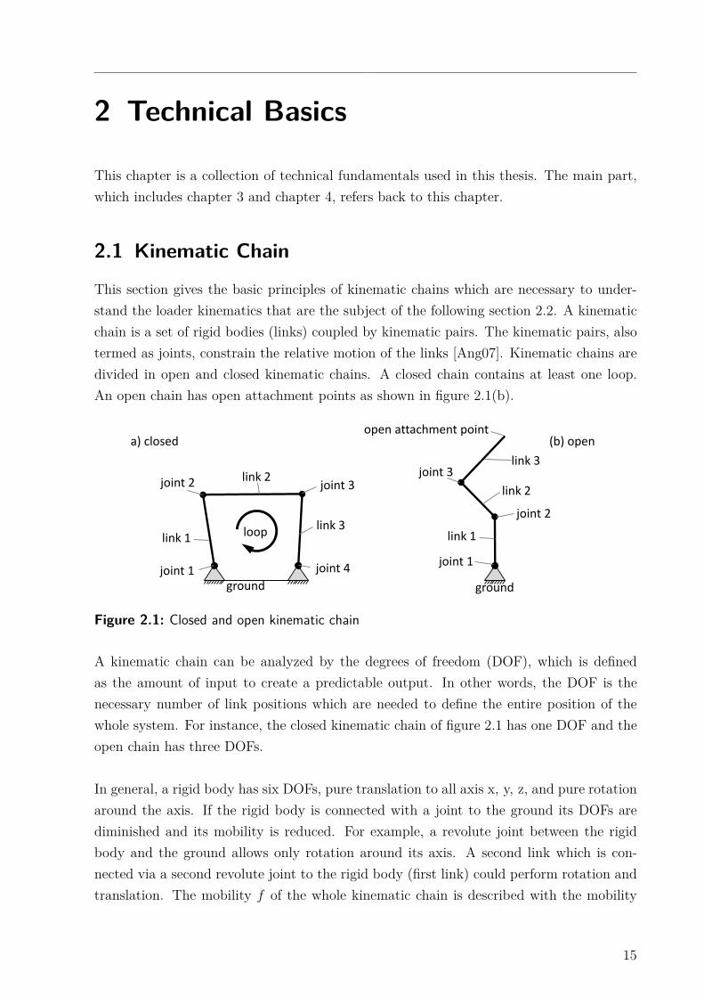
This section gives the basic principles of kinematic chains which are necessary to under-
stand the loader kinematics that are the subject of the following section 2.2. A kinematic
chain is a set of rigid bodies (links) coupled by kinematic pairs. The kinematic pairs, also
termed as joints, constrain the relative motion of the links [Ang07]. Kinematic chains are
divided in open and closed kinematic chains. A closed chain contains at least one loop.
An open chain has open attachment points as shown in figure 2.1(b).
link 1
joint 1
link 2
link 3
joint 2 joint 3
joint 4
ground
loop
ground
joint 1
link 1
joint 2
link 2
link 3joint 3
open attachment point(a) closed (b) open
Figure 2.1: Closed and open kinematic chain
A kinematic chain can be analyzed by the degrees of freedom (DOF), which is defined
as the amount of input to create a predictable output. In other words, the DOF is the
necessary number of link positions which are needed to define the entire position of the
whole system. For instance, the closed kinematic chain of figure 2.1 has one DOF and the
open chain has three DOFs.
In general, a rigid body has six DOFs, pure translation to all axis x, y, z, and pure rotation
around the axis. If the rigid body is connected with a joint to the ground its DOFs are
diminished and its mobility is reduced. For example, a revolute joint between the rigid
body and the ground allows only rotation around its axis. A second link which is con-
nected via a second revolute joint to the rigid body (first link) could perform rotation and
translation. The mobility f of the whole kinematic chain is described with the mobility
15
2 Technical Basics
table [Mar05] which specifies f = 3 for planar chains. The number of DOFs is calculated
by the following equation:
DOF = (6 − f)n −5∑
j=f+1
[(j − f)cj] (2.1)
Here, the number of linkages equal n, the number of joints per type equal c, and the num-
ber of diminished DOFs equal j according to the joint type. For example, a revolute joint
has one DOF, that means five DOFs are diminished, hence, j = 5. Another example is the
closed kinematic chain of figure 2.1(a) which has four joints of one DOF, thus, j = 5 and
c5 = 4.
The joint order increases by one for every additionally connected link as shown in fig-
ure 2.2. For instance, a first order joint connects two links and counts as a single joint
c = 1. A second order joint connects three links and counts twice, hence, c = 2 and so
forth [Mar05] [GHSW06].
link 1 link 2
first order joint
link 1link 3
link 2
second order joint
Figure 2.2: Joint order
1st order joint
2nd order joint
3rd order joint
(a) (b) (c)
Figure 2.3: Transfer contour to linkage
A link with more than two joints is termed as contour, figure 2.3(a). To calculate the DOFs
of the kinematic chain, the contour is transferred into a linkage via connecting the joints
of the contour with links, as shown in figure 2.3(b). For the resulting kinematic chain of
figure 2.3(c) follows, with f = 3, n = 5, c5 = 7, and equation (2.1):
DOF = (6 − 3)5 − [(5 − 3)7] = 1 (2.2)
16
2.2 Loader Kinematics
2.2 Loader Kinematics
This section analyzes the kinematics of loaders. The loaders shown here in 2D represent
commonly 80% of the available loaders.
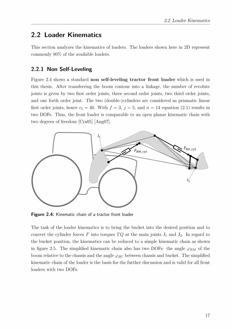
2.2.1 Non Self-Leveling
Figure 2.4 shows a standard non self-leveling tractor front loader which is used in
this thesis. After transferring the boom contour into a linkage, the number of revolute
joints is given by two first order joints, three second order joints, two third order joints,
and one forth order joint. The two (double-)cylinders are considered as prismatic linear
first order joints, hence c5 = 40. With f = 3, j = 5, and n = 14 equation (2.1) results in
two DOFs. Thus, the front loader is comparable to an open planar kinematic chain with
two degrees of freedom [Cra05] [Ang07].
J1
J2
���_ ���_
Figure 2.4: Kinematic chain of a tractor front loader
The task of the loader kinematics is to bring the bucket into the desired position and to
convert the cylinder forces F into torques TQ at the main joints J1 and J2. In regard to
the bucket position, the kinematics can be reduced to a simple kinematic chain as shown
in figure 2.5. The simplified kinematic chain also has two DOFs: the angle ϕBM of the
boom relative to the chassis and the angle ϕBU between chassis and bucket. The simplified
kinematic chain of the loader is the basis for the further discussion and is valid for all front
loaders with two DOFs.
17
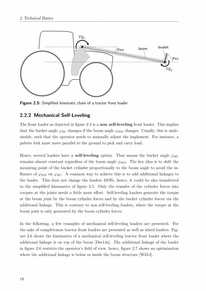
2 Technical Basics
��� ���boom bucket
Figure 2.5: Simplified kinematic chain of a tractor front loader
2.2.2 Mechanical Self-Leveling
The front loader as depicted in figure 2.4 is a non self-leveling front loader. This implies
that the bucket angle ϕBU changes if the boom angle ϕBM changes. Usually, this is unde-
sirable, such that the operator needs to manually adjust the implement. For instance, a
palette fork must move parallel to the ground to pick and carry load.
Hence, several loaders have a self-leveling option. That means the bucket angle ϕBU
remains almost constant regardless of the boom angle ϕBM . The key idea is to shift the
mounting point of the bucket cylinder proportionally to the boom angle to avoid the in-
fluence of ϕBM on ϕBU . A common way to achieve this is to add additional linkages to
the loader. This does not change the loaders DOFs, hence, it could be also transferred
to the simplified kinematics of figure 2.5. Only the transfer of the cylinder forces into
torques at the joints needs a little more effort. Self-leveling loaders generate the torque
at the boom joint by the boom cylinder forces and by the bucket cylinder forces via the
additional linkage. This is contrary to non self-leveling loaders, where the torque at the
boom joint is only generated by the boom cylinder forces.
In the following, a few examples of mechanical self-leveling loaders are presented. For
the sake of completeness tractor front loaders are presented as well as wheel loaders. Fig-
ure 2.6 shows the kinematics of a mechanical self-leveling tractor front loader where the
additional linkage is on top of the boom [Dee14a]. The additional linkage of the loader
in figure 2.6 restricts the operator’s field of view, hence, figure 2.7 shows an optimization
where the additional linkage is below or inside the boom structure [Wil14].
18
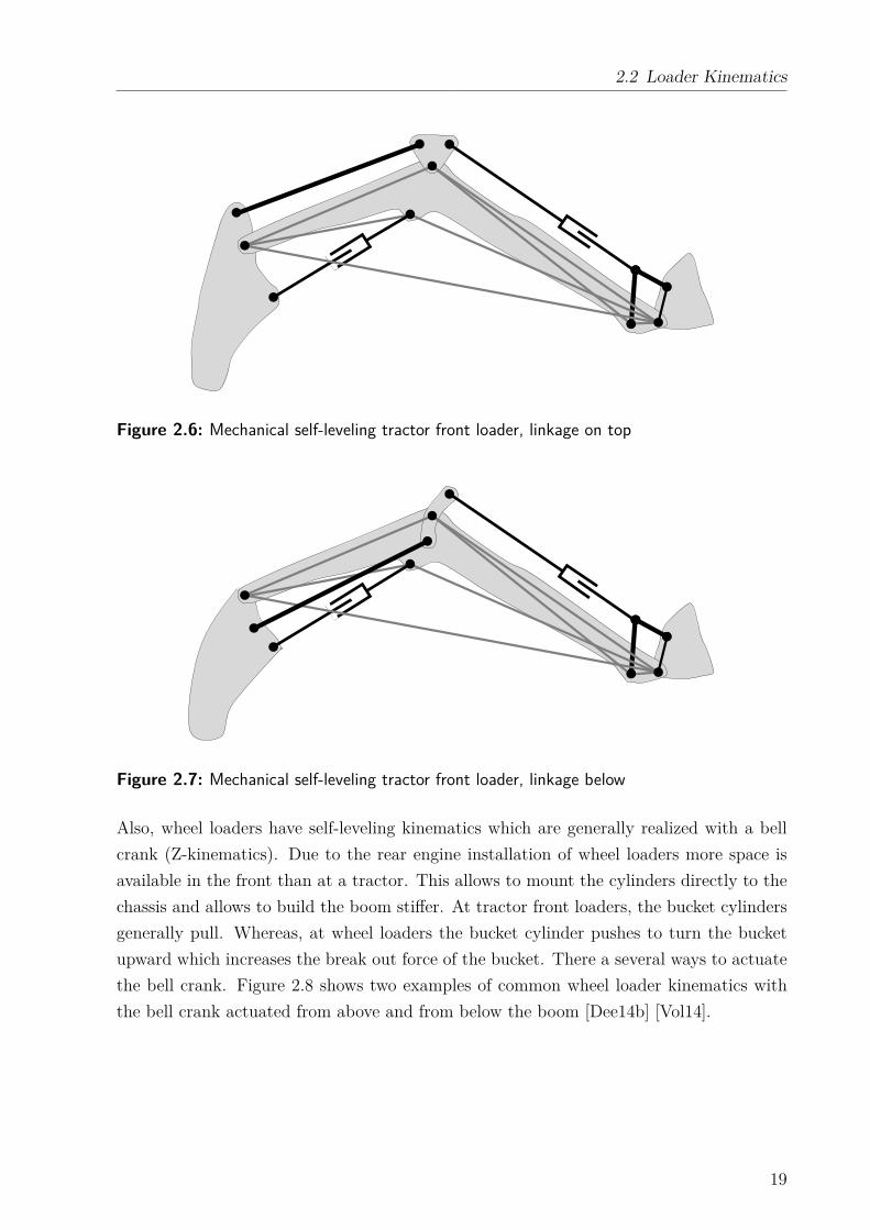
2.2 Loader Kinematics
Figure 2.6: Mechanical self-leveling tractor front loader, linkage on top
Figure 2.7: Mechanical self-leveling tractor front loader, linkage below
Also, wheel loaders have self-leveling kinematics which are generally realized with a bell
crank (Z-kinematics). Due to the rear engine installation of wheel loaders more space is
available in the front than at a tractor. This allows to mount the cylinders directly to the
chassis and allows to build the boom stiffer. At tractor front loaders, the bucket cylinders
generally pull. Whereas, at wheel loaders the bucket cylinder pushes to turn the bucket
upward which increases the break out force of the bucket. There a several ways to actuate
the bell crank. Figure 2.8 shows two examples of common wheel loader kinematics with
the bell crank actuated from above and from below the boom [Dee14b] [Vol14].
19
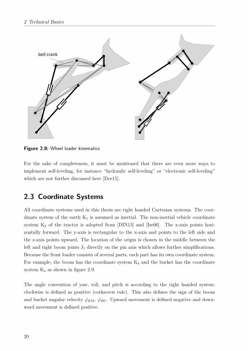
2 Technical Basics
bell crank
Figure 2.8: Wheel loader kinematics
For the sake of completeness, it must be mentioned that there are even more ways to
implement self-leveling, for instance “hydraulic self-leveling” or “electronic self-leveling”
which are not further discussed here [Dee15].
2.3 Coordinate Systems
All coordinate systems used in this thesis are right handed Cartesian systems. The coor-
dinate system of the earth K1 is assumed as inertial. The non-inertial vehicle coordinate
system K2 of the tractor is adopted from [DIN13] and [Ise06]. The x-axis points hori-
zontally forward. The y-axis is rectangular to the x-axis and points to the left side and
the z-axis points upward. The location of the origin is chosen in the middle between the
left and right boom joints J1 directly on the pin axis which allows further simplifications.
Because the front loader consists of several parts, each part has its own coordinate system.
For example, the boom has the coordinate system K3 and the bucket has the coordinate
system K4 as shown in figure 2.9.
The angle convention of yaw, roll, and pitch is according to the right handed system:
clockwise is defined as positive (corkscrew rule). This also defines the sign of the boom
and bucket angular velocity ϕBM , ϕBU . Upward movement is defined negative and down-
ward movement is defined positive.
20
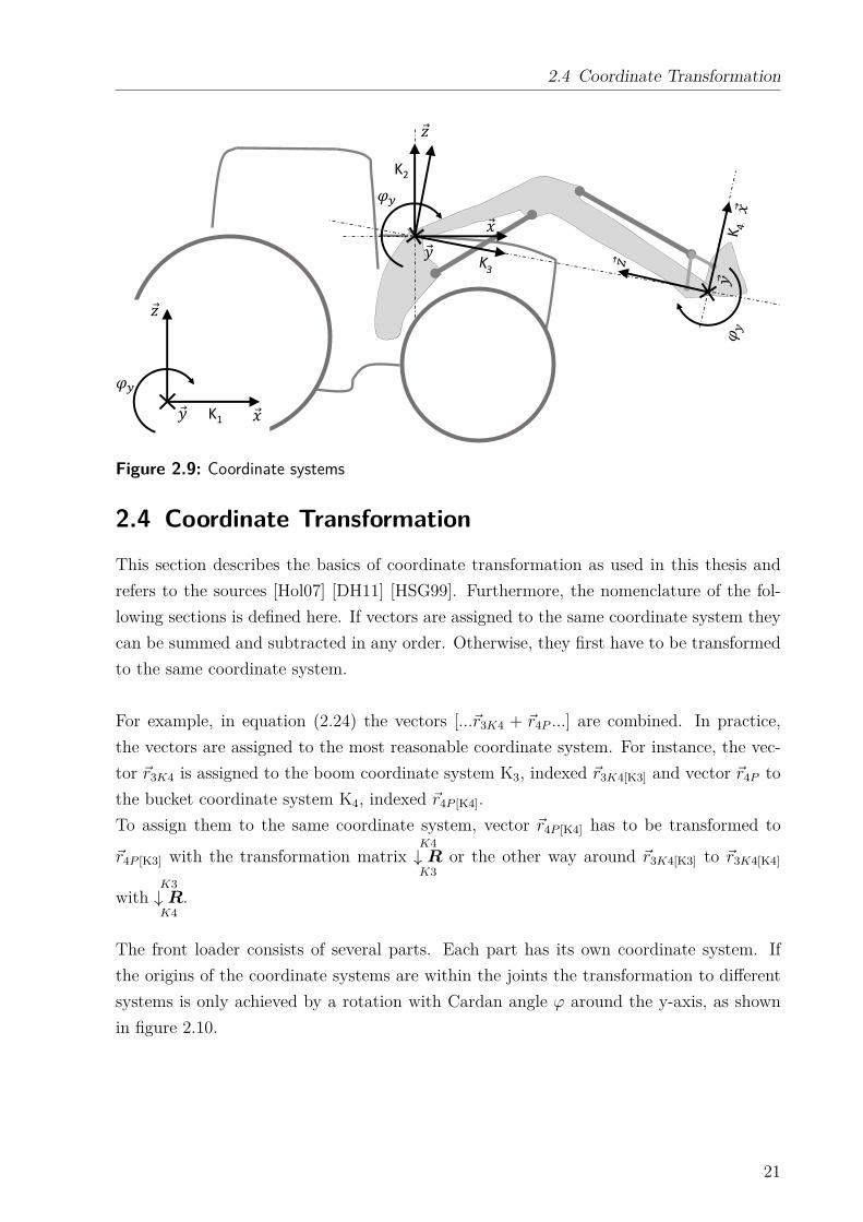
2.4 Coordinate Transformation
� � �
K1
� �
� K2
Figure 2.9: Coordinate systems
2.4 Coordinate Transformation
This section describes the basics of coordinate transformation as used in this thesis and
refers to the sources [Hol07] [DH11] [HSG99]. Furthermore, the nomenclature of the fol-
lowing sections is defined here. If vectors are assigned to the same coordinate system they
can be summed and subtracted in any order. Otherwise, they first have to be transformed
to the same coordinate system.
For example, in equation (2.24) the vectors [...~r3K4 + ~r4P ...] are combined. In practice,
the vectors are assigned to the most reasonable coordinate system. For instance, the vec-
tor ~r3K4 is assigned to the boom coordinate system K3, indexed ~r3K4[K3] and vector ~r4P to
the bucket coordinate system K4, indexed ~r4P [K4].
To assign them to the same coordinate system, vector ~r4P [K4] has to be transformed to
~r4P [K3] with the transformation matrixK4
↓ RK3
or the other way around ~r3K4[K3] to ~r3K4[K4]
withK3
↓ RK4
.
The front loader consists of several parts. Each part has its own coordinate system. If
the origins of the coordinate systems are within the joints the transformation to different
systems is only achieved by a rotation with Cardan angle ϕ around the y-axis, as shown
in figure 2.10.
21
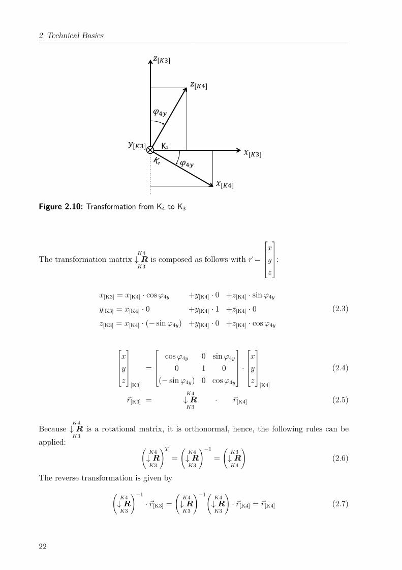
2 Technical Basics
K1
�� �[� ]
�[� ] �[� ]
�[� ][� ]
Figure 2.10: Transformation from K4 to K3
The transformation matrixK4
↓ RK3
is composed as follows with ~r =
x
y
z
:
x[K3] = x[K4] · cos ϕ4y +y[K4] · 0 +z[K4] · sin ϕ4y
y[K3] = x[K4] · 0 +y[K4] · 1 +z[K4] · 0
z[K3] = x[K4] · (− sin ϕ4y) +y[K4] · 0 +z[K4] · cos ϕ4y
(2.3)
x
y
z
[K3]
=
cos ϕ4y 0 sin ϕ4y
0 1 0
(− sin ϕ4y) 0 cos ϕ4y
·
x
y
z
[K4]
(2.4)
~r[K3] =K4
↓ RK3
· ~r[K4] (2.5)
BecauseK4
↓ RK3
is a rotational matrix, it is orthonormal, hence, the following rules can be
applied:(
K4
↓ RK3
)T
=
(
K4
↓ RK3
)−1
=
(
K3
↓ RK4
)
(2.6)
The reverse transformation is given by
(
K4
↓ RK3
)−1
· ~r[K3] =
(
K4
↓ RK3
)−1(K4
↓ RK3
)
· ~r[K4] = ~r[K4] (2.7)
22
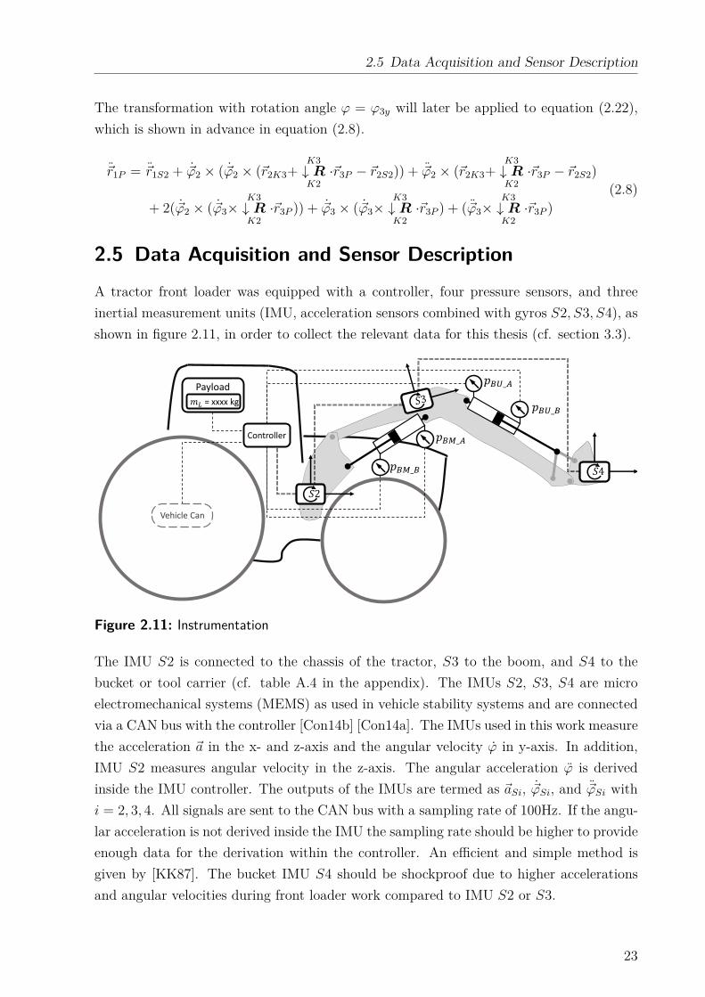
2.5 Data Acquisition and Sensor Description
The transformation with rotation angle ϕ = ϕ3y will later be applied to equation (2.22),
which is shown in advance in equation (2.8).
~r1P = ~r1S2 + ~ϕ2 × ( ~ϕ2 × (~r2K3+K3
↓ RK2
·~r3P − ~r2S2)) + ~ϕ2 × (~r2K3+K3
↓ RK2
·~r3P − ~r2S2)
+ 2( ~ϕ2 × ( ~ϕ3×K3
↓ RK2
·~r3P )) + ~ϕ3 × ( ~ϕ3×K3
↓ RK2
·~r3P ) + ( ~ϕ3×K3
↓ RK2
·~r3P )(2.8)
2.5 Data Acquisition and Sensor Description
A tractor front loader was equipped with a controller, four pressure sensors, and three
inertial measurement units (IMU, acceleration sensors combined with gyros S2, S3, S4), as
shown in figure 2.11, in order to collect the relevant data for this thesis (cf. section 3.3).
��_��_�
Payload
= xxxx kg
Vehicle Can
Controller
��_��_�
2 4
Figure 2.11: Instrumentation
The IMU S2 is connected to the chassis of the tractor, S3 to the boom, and S4 to the
bucket or tool carrier (cf. table A.4 in the appendix). The IMUs S2, S3, S4 are micro
electromechanical systems (MEMS) as used in vehicle stability systems and are connected
via a CAN bus with the controller [Con14b] [Con14a]. The IMUs used in this work measure
the acceleration ~a in the x- and z-axis and the angular velocity ϕ in y-axis. In addition,
IMU S2 measures angular velocity in the z-axis. The angular acceleration ϕ is derived
inside the IMU controller. The outputs of the IMUs are termed as ~aSi, ~ϕSi, and ~ϕSi with
i = 2, 3, 4. All signals are sent to the CAN bus with a sampling rate of 100Hz. If the angu-
lar acceleration is not derived inside the IMU the sampling rate should be higher to provide
enough data for the derivation within the controller. An efficient and simple method is
given by [KK87]. The bucket IMU S4 should be shockproof due to higher accelerations
and angular velocities during front loader work compared to IMU S2 or S3.
23
2 Technical Basics
The pressure sensors measure cylinder pressures at the piston and at the rod side of the
boom and bucket cylinders. The best way to do this, is by measuring the pressure directly
within the cylinder to avoid pressure drop deviations due to oil flow. This could not be
realized. Thus, the sensors are connected with a T-fitting and a 90 degree knee fitting
(size: 13/16"-16UN) in the hydraulic line just next to the cylinder ports. This keeps the
deviation of the pressure drop due to the oil flow negligibly small. The sensors deliver an
analogous voltage signal and are connected directly to the controller. For this reason the
pressure readings are transferred faster than the accelerations from the CAN bus. Given
that the signals of all sensors are used for further calculations, they have to be synchronized
first. Hence, the analogous pressure inputs are provided with a time lag.
Additionally, the hydraulic oil temperature or engine speed, for example, are derived from
the vehicle CAN bus. Finally, all data is processed in a real time controller to calcu-
late the payload with a sample time of 10 milliseconds. The used controller is a real
time rapid prototyping system (dSPACE MicroAutoBox2 [dSP14]) which is programmed
directly with Matlab/Simulink. It enables, among other things, recording variables and
debugging while simultaneously displaying the variables on a notebook (see also section
A.2 in the appendix).
2.6 Accelerations
This section summarizes the essentials of accelerations as a basis of this thesis and refers
to the sources [Hon93][Sch07][Nol06][HSG99]. The Position Detection of chapter 3 as well
as the Weighing Function of chapter 4 are parameterized with continuously measured ac-
celerations. This requires a comprehensive understanding and detailed explanation. In
the following, the accelerations of any point, which is referenced to different coordinate
systems, are explained in general. In a second step, the point is associated with the loader
and represents, for example, the center of gravity of a specific part. Finally, this section
explains how to calculate the acceleration of this point by measuring accelerations at a dif-
ferent position. For reasons of clarity and ease of comprehension, all figures in this section
are based on two dimensions. In addition, vector ~r1(t) will be written as ~r1. For further
calculations, all vectors have to be first transformed to the same coordinate system, e.g.
~r1P = ~r1K2+K2
↓ RK1
~r2P (cf. figure 2.13). In addition, the transformation matricesK∗
↓ RK∗
in the
equations of this chapter are omitted for reasons of clarity.
The coordinate system K1 (see figure 2.12) is an inertial system also known as inertial
24
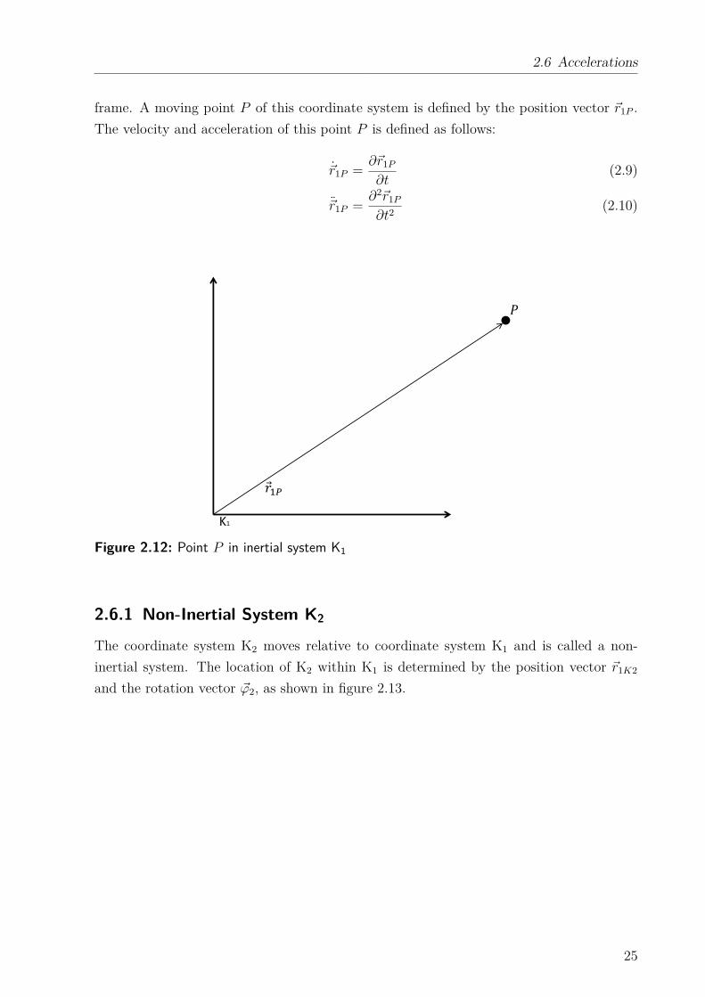
2.6 Accelerations
frame. A moving point P of this coordinate system is defined by the position vector ~r1P .
The velocity and acceleration of this point P is defined as follows:
~r1P =∂~r1P
∂t(2.9)
~r1P =∂2~r1P
∂t2(2.10)
K1
�Figure 2.12: Point P in inertial system K1
2.6.1 Non-Inertial System K2
The coordinate system K2 moves relative to coordinate system K1 and is called a non-
inertial system. The location of K2 within K1 is determined by the position vector ~r1K2
and the rotation vector ~ϕ2, as shown in figure 2.13.
25
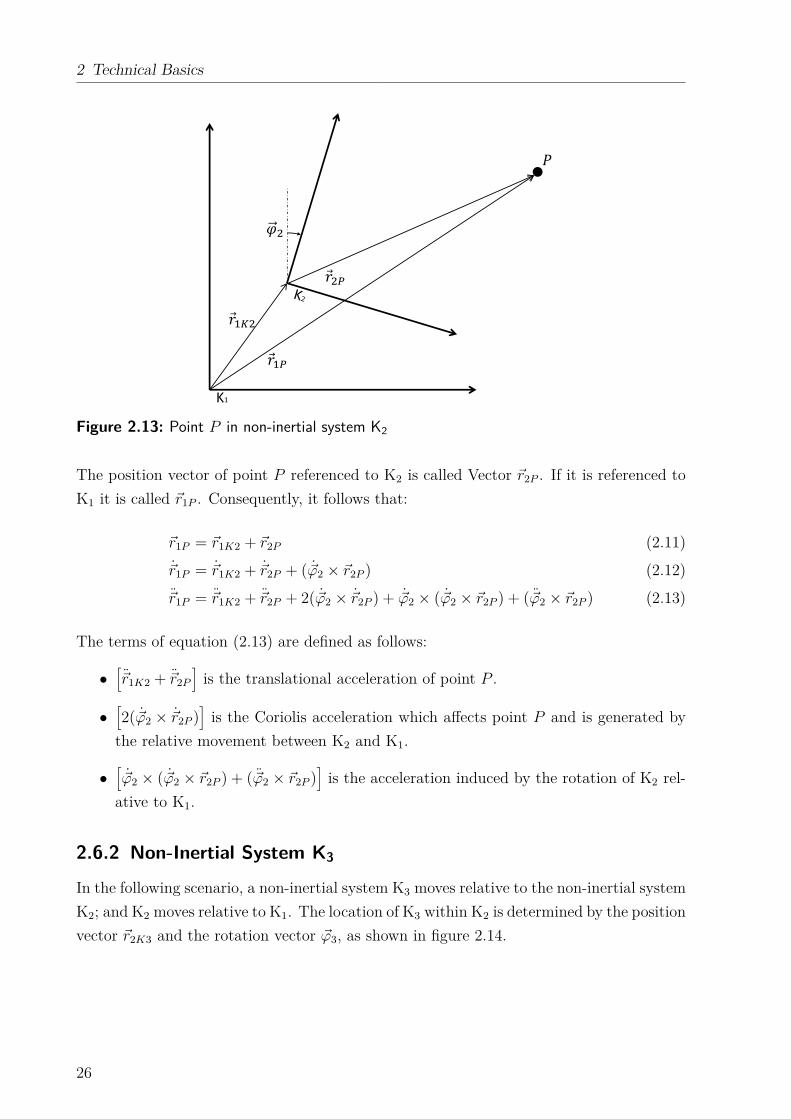
2 Technical Basics
K1
� �
� � �
Figure 2.13: Point P in non-inertial system K2
The position vector of point P referenced to K2 is called Vector ~r2P . If it is referenced to
K1 it is called ~r1P . Consequently, it follows that:
~r1P = ~r1K2 + ~r2P (2.11)
~r1P = ~r1K2 + ~r2P + ( ~ϕ2 × ~r2P ) (2.12)
~r1P = ~r1K2 + ~r2P + 2( ~ϕ2 × ~r2P ) + ~ϕ2 × ( ~ϕ2 × ~r2P ) + ( ~ϕ2 × ~r2P ) (2.13)
The terms of equation (2.13) are defined as follows:
•[
~r1K2 + ~r2P
]
is the translational acceleration of point P .
•[
2( ~ϕ2 × ~r2P )]
is the Coriolis acceleration which affects point P and is generated by
the relative movement between K2 and K1.
•[
~ϕ2 × ( ~ϕ2 × ~r2P ) + ( ~ϕ2 × ~r2P )]
is the acceleration induced by the rotation of K2 rel-
ative to K1.
2.6.2 Non-Inertial System K3
In the following scenario, a non-inertial system K3 moves relative to the non-inertial system
K2; and K2 moves relative to K1. The location of K3 within K2 is determined by the position
vector ~r2K3 and the rotation vector ~ϕ3, as shown in figure 2.14.
26
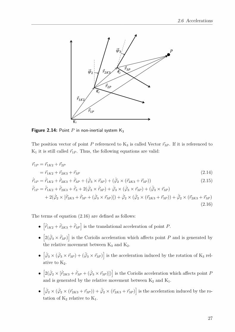
2.6 Accelerations
K1
� �
���
� � � �
Figure 2.14: Point P in non-inertial system K3
The position vector of point P referenced to K3 is called Vector ~r3P . If it is referenced to
K1 it is still called ~r1P . Thus, the following equations are valid:
~r1P = ~r1K2 + ~r2P
= ~r1K2 + ~r2K3 + ~r3P (2.14)
~r1P = ~r1K2 + ~r2K3 + ~r3P + ( ~ϕ3 × ~r3P ) + ( ~ϕ2 × (~r2K3 + ~r3P )) (2.15)
~r1P = ~r1K2 + ~r2K3 + ~r3 + 2( ~ϕ3 × ~r3P ) + ~ϕ3 × ( ~ϕ3 × ~r3P ) + ( ~ϕ3 × ~r3P )
+ 2( ~ϕ2 × [~r2K3 + ~r3P + ( ~ϕ3 × ~r3P )]) + ~ϕ2 × ( ~ϕ2 × (~r2K3 + ~r3P )) + ~ϕ2 × (~r2K3 + ~r3P )
(2.16)
The terms of equation (2.16) are defined as follows:
•[
~r1K2 + ~r2K3 + ~r3P
]
is the translational acceleration of point P .
•[
2( ~ϕ3 × ~r3P )]
is the Coriolis acceleration which affects point P and is generated by
the relative movement between K3 and K2.
•[
~ϕ3 × ( ~ϕ3 × ~r3P ) + ( ~ϕ3 × ~r3P )]
is the acceleration induced by the rotation of K3 rel-
ative to K2.
•[
2( ~ϕ2 × [~r2K3 + ~r3P + ( ~ϕ3 × ~r3P )])]
is the Coriolis acceleration which affects point P
and is generated by the relative movement between K2 and K1.
•[
~ϕ2 × ( ~ϕ2 × (~r2K3 + ~r3P )) + ~ϕ2 × (~r2K3 + ~r3P )]
is the acceleration induced by the ro-
tation of K2 relative to K1.
27
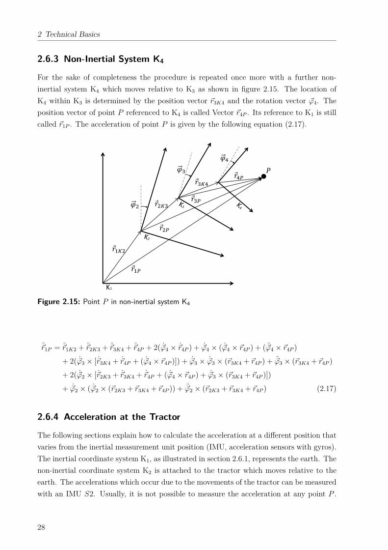
2 Technical Basics
2.6.3 Non-Inertial System K4
For the sake of completeness the procedure is repeated once more with a further non-
inertial system K4 which moves relative to K3 as shown in figure 2.15. The location of
K4 within K3 is determined by the position vector ~r3K4 and the rotation vector ~ϕ4. The
position vector of point P referenced to K4 is called Vector ~r4P . Its reference to K1 is still
called ~r1P . The acceleration of point P is given by the following equation (2.17).
K1
� �
� �
�� �
� � � �
� �
Figure 2.15: Point P in non-inertial system K4
~r1P = ~r1K2 + ~r2K3 + ~r3K4 + ~r4P + 2( ~ϕ4 × ~r4P ) + ~ϕ4 × ( ~ϕ4 × ~r4P ) + ( ~ϕ4 × ~r4P )
+ 2( ~ϕ3 × [~r3K4 + ~r4P + ( ~ϕ4 × ~r4P )]) + ~ϕ3 × ~ϕ3 × (~r3K4 + ~r4P ) + ~ϕ3 × (~r3K4 + ~r4P )
+ 2( ~ϕ2 × [~r2K3 + ~r3K4 + ~r4P + ( ~ϕ4 × ~r4P ) + ~ϕ3 × (~r3K4 + ~r4P )])
+ ~ϕ2 × ( ~ϕ2 × (~r2K3 + ~r3K4 + ~r4P )) + ~ϕ2 × (~r2K3 + ~r3K4 + ~r4P ) (2.17)
2.6.4 Acceleration at the Tractor
The following sections explain how to calculate the acceleration at a different position that
varies from the inertial measurement unit position (IMU, acceleration sensors with gyros).
The inertial coordinate system K1, as illustrated in section 2.6.1, represents the earth. The
non-inertial coordinate system K2 is attached to the tractor which moves relative to the
earth. The accelerations which occur due to the movements of the tractor can be measured
with an IMU S2. Usually, it is not possible to measure the acceleration at any point P .
28
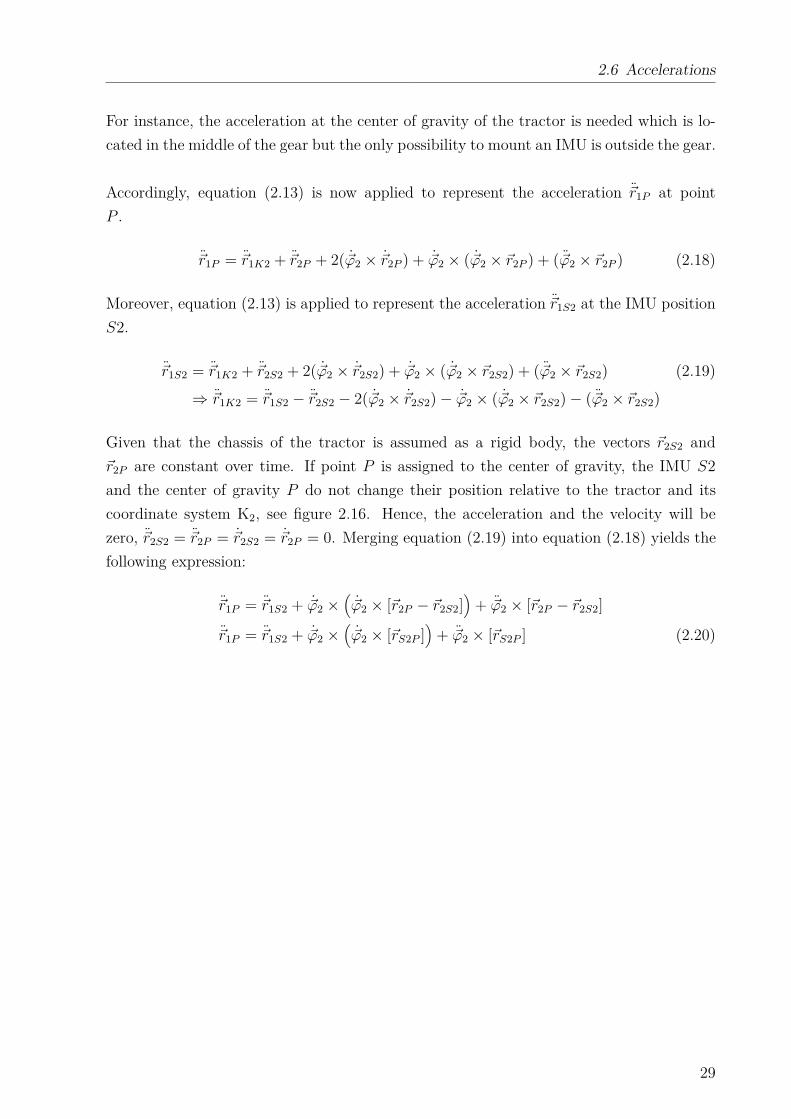
2.6 Accelerations
For instance, the acceleration at the center of gravity of the tractor is needed which is lo-
cated in the middle of the gear but the only possibility to mount an IMU is outside the gear.
Accordingly, equation (2.13) is now applied to represent the acceleration ~r1P at point
P .
~r1P = ~r1K2 + ~r2P + 2( ~ϕ2 × ~r2P ) + ~ϕ2 × ( ~ϕ2 × ~r2P ) + ( ~ϕ2 × ~r2P ) (2.18)
Moreover, equation (2.13) is applied to represent the acceleration ~r1S2 at the IMU position
S2.
~r1S2 = ~r1K2 + ~r2S2 + 2( ~ϕ2 × ~r2S2) + ~ϕ2 × ( ~ϕ2 × ~r2S2) + ( ~ϕ2 × ~r2S2) (2.19)
⇒ ~r1K2 = ~r1S2 − ~r2S2 − 2( ~ϕ2 × ~r2S2) − ~ϕ2 × ( ~ϕ2 × ~r2S2) − ( ~ϕ2 × ~r2S2)
Given that the chassis of the tractor is assumed as a rigid body, the vectors ~r2S2 and
~r2P are constant over time. If point P is assigned to the center of gravity, the IMU S2
and the center of gravity P do not change their position relative to the tractor and its
coordinate system K2, see figure 2.16. Hence, the acceleration and the velocity will be
zero, ~r2S2 = ~r2P = ~r2S2 = ~r2P = 0. Merging equation (2.19) into equation (2.18) yields the
following expression:
~r1P = ~r1S2 + ~ϕ2 ×(
~ϕ2 × [~r2P − ~r2S2])
+ ~ϕ2 × [~r2P − ~r2S2]
~r1P = ~r1S2 + ~ϕ2 ×(
~ϕ2 × [~rS2P ])
+ ~ϕ2 × [~rS2P ] (2.20)
29
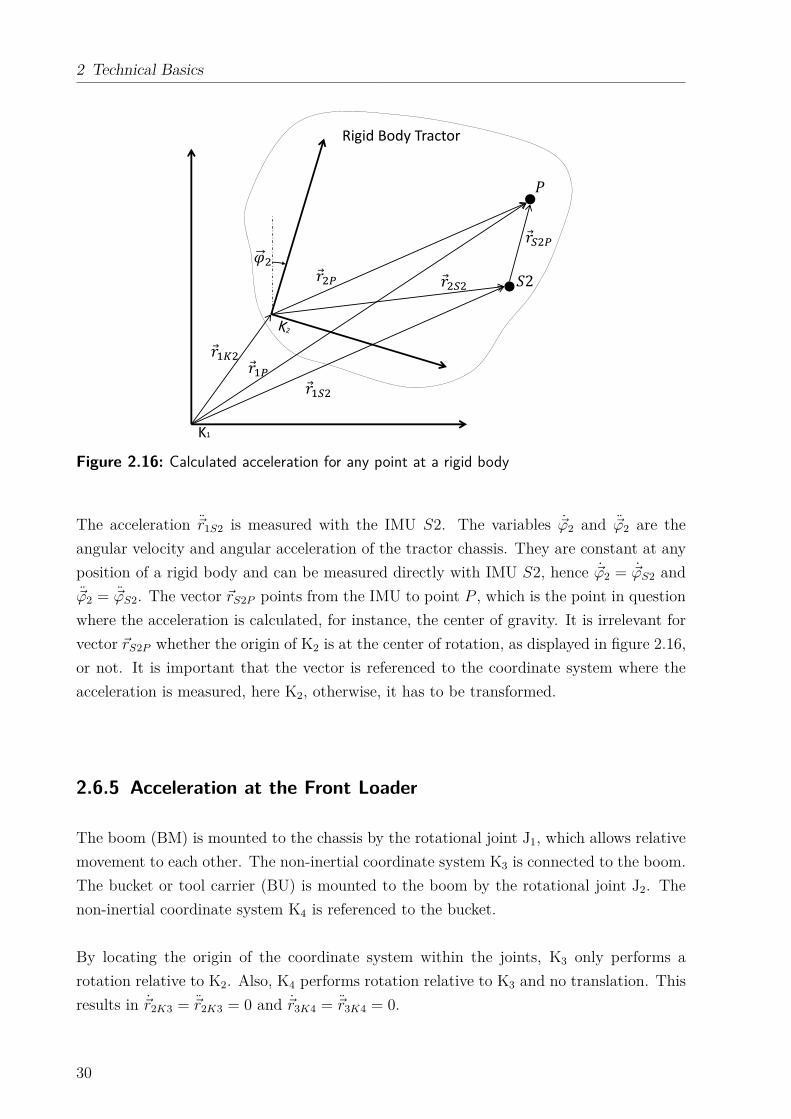
2 Technical Basics
K1
� �� 2
� �
Rigid Body Tractor
� �
�
Figure 2.16: Calculated acceleration for any point at a rigid body
The acceleration ~r1S2 is measured with the IMU S2. The variables ~ϕ2 and ~ϕ2 are the
angular velocity and angular acceleration of the tractor chassis. They are constant at any
position of a rigid body and can be measured directly with IMU S2, hence ~ϕ2 = ~ϕS2 and
~ϕ2 = ~ϕS2. The vector ~rS2P points from the IMU to point P , which is the point in question
where the acceleration is calculated, for instance, the center of gravity. It is irrelevant for
vector ~rS2P whether the origin of K2 is at the center of rotation, as displayed in figure 2.16,
or not. It is important that the vector is referenced to the coordinate system where the
acceleration is measured, here K2, otherwise, it has to be transformed.
2.6.5 Acceleration at the Front Loader
The boom (BM) is mounted to the chassis by the rotational joint J1, which allows relative
movement to each other. The non-inertial coordinate system K3 is connected to the boom.
The bucket or tool carrier (BU) is mounted to the boom by the rotational joint J2. The
non-inertial coordinate system K4 is referenced to the bucket.
By locating the origin of the coordinate system within the joints, K3 only performs a
rotation relative to K2. Also, K4 performs rotation relative to K3 and no translation. This
results in ~r2K3 = ~r2K3 = 0 and ~r3K4 = ~r3K4 = 0.
30
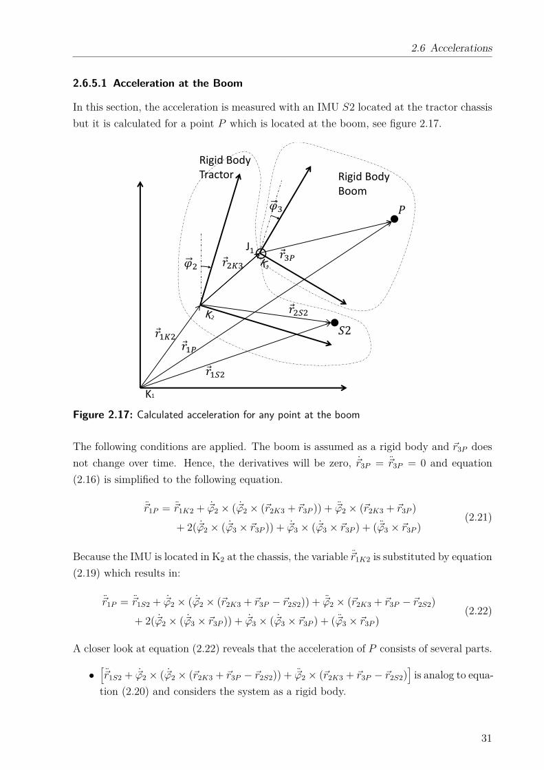
2.6 Accelerations
2.6.5.1 Acceleration at the Boom
In this section, the acceleration is measured with an IMU S2 located at the tractor chassis
but it is calculated for a point P which is located at the boom, see figure 2.17.
K1
��
�Rigid Body
Tractor Rigid Body
Boom
� � 2
J1 � � �
� �
Figure 2.17: Calculated acceleration for any point at the boom
The following conditions are applied. The boom is assumed as a rigid body and ~r3P does
not change over time. Hence, the derivatives will be zero, ~r3P = ~r3P = 0 and equation
(2.16) is simplified to the following equation.
~r1P = ~r1K2 + ~ϕ2 × ( ~ϕ2 × (~r2K3 + ~r3P )) + ~ϕ2 × (~r2K3 + ~r3P )
+ 2( ~ϕ2 × ( ~ϕ3 × ~r3P )) + ~ϕ3 × ( ~ϕ3 × ~r3P ) + ( ~ϕ3 × ~r3P )(2.21)
Because the IMU is located in K2 at the chassis, the variable ~r1K2 is substituted by equation
(2.19) which results in:
~r1P = ~r1S2 + ~ϕ2 × ( ~ϕ2 × (~r2K3 + ~r3P − ~r2S2)) + ~ϕ2 × (~r2K3 + ~r3P − ~r2S2)
+ 2( ~ϕ2 × ( ~ϕ3 × ~r3P )) + ~ϕ3 × ( ~ϕ3 × ~r3P ) + ( ~ϕ3 × ~r3P )(2.22)
A closer look at equation (2.22) reveals that the acceleration of P consists of several parts.
•[
~r1S2 + ~ϕ2 × ( ~ϕ2 × (~r2K3 + ~r3P − ~r2S2)) + ~ϕ2 × (~r2K3 + ~r3P − ~r2S2)]
is analog to equa-
tion (2.20) and considers the system as a rigid body.
31
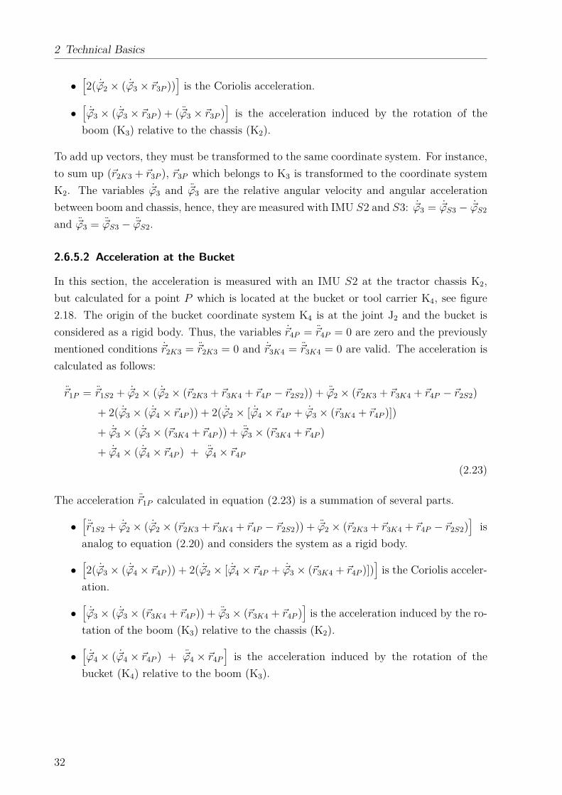
2 Technical Basics
•[
2( ~ϕ2 × ( ~ϕ3 × ~r3P ))]
is the Coriolis acceleration.
•[
~ϕ3 × ( ~ϕ3 × ~r3P ) + ( ~ϕ3 × ~r3P )]
is the acceleration induced by the rotation of the
boom (K3) relative to the chassis (K2).
To add up vectors, they must be transformed to the same coordinate system. For instance,
to sum up (~r2K3 + ~r3P ), ~r3P which belongs to K3 is transformed to the coordinate system
K2. The variables ~ϕ3 and ~ϕ3 are the relative angular velocity and angular acceleration
between boom and chassis, hence, they are measured with IMU S2 and S3: ~ϕ3 = ~ϕS3 − ~ϕS2
and ~ϕ3 = ~ϕS3 − ~ϕS2.
2.6.5.2 Acceleration at the Bucket
In this section, the acceleration is measured with an IMU S2 at the tractor chassis K2,
but calculated for a point P which is located at the bucket or tool carrier K4, see figure
2.18. The origin of the bucket coordinate system K4 is at the joint J2 and the bucket is
considered as a rigid body. Thus, the variables ~r4P = ~r4P = 0 are zero and the previously
mentioned conditions ~r2K3 = ~r2K3 = 0 and ~r3K4 = ~r3K4 = 0 are valid. The acceleration is
calculated as follows:
~r1P = ~r1S2 + ~ϕ2 × ( ~ϕ2 × (~r2K3 + ~r3K4 + ~r4P − ~r2S2)) + ~ϕ2 × (~r2K3 + ~r3K4 + ~r4P − ~r2S2)
+ 2( ~ϕ3 × ( ~ϕ4 × ~r4P )) + 2( ~ϕ2 × [ ~ϕ4 × ~r4P + ~ϕ3 × (~r3K4 + ~r4P )])
+ ~ϕ3 × ( ~ϕ3 × (~r3K4 + ~r4P )) + ~ϕ3 × (~r3K4 + ~r4P )
+ ~ϕ4 × ( ~ϕ4 × ~r4P ) + ~ϕ4 × ~r4P
(2.23)
The acceleration ~r1P calculated in equation (2.23) is a summation of several parts.
•[
~r1S2 + ~ϕ2 × ( ~ϕ2 × (~r2K3 + ~r3K4 + ~r4P − ~r2S2)) + ~ϕ2 × (~r2K3 + ~r3K4 + ~r4P − ~r2S2)]
is
analog to equation (2.20) and considers the system as a rigid body.
•[
2( ~ϕ3 × ( ~ϕ4 × ~r4P )) + 2( ~ϕ2 × [ ~ϕ4 × ~r4P + ~ϕ3 × (~r3K4 + ~r4P )])]
is the Coriolis acceler-
ation.
•[
~ϕ3 × ( ~ϕ3 × (~r3K4 + ~r4P )) + ~ϕ3 × (~r3K4 + ~r4P )]
is the acceleration induced by the ro-
tation of the boom (K3) relative to the chassis (K2).
•[
~ϕ4 × ( ~ϕ4 × ~r4P ) + ~ϕ4 × ~r4P
]
is the acceleration induced by the rotation of the
bucket (K4) relative to the boom (K3).
32
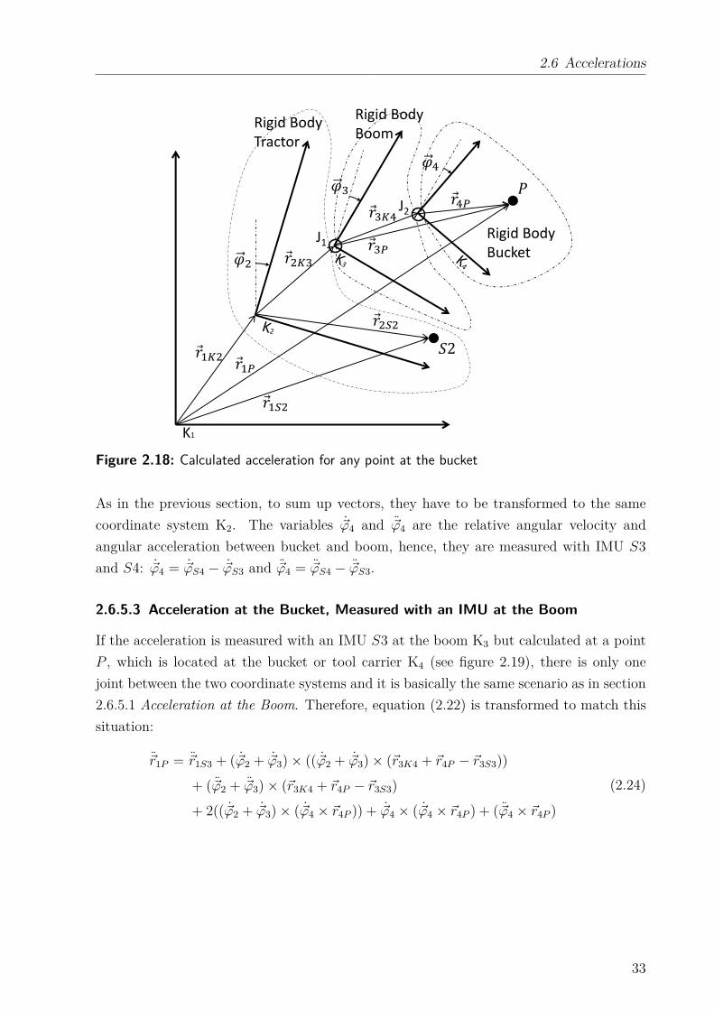
2.6 Accelerations
K1
�
� �
�� �
� � 2
Rigid Body
Tractor
Rigid Body
Boom
Rigid Body
BucketJ1
J2
� � � �
� �
Figure 2.18: Calculated acceleration for any point at the bucket
As in the previous section, to sum up vectors, they have to be transformed to the same
coordinate system K2. The variables ~ϕ4 and ~ϕ4 are the relative angular velocity and
angular acceleration between bucket and boom, hence, they are measured with IMU S3
and S4: ~ϕ4 = ~ϕS4 − ~ϕS3 and ~ϕ4 = ~ϕS4 − ~ϕS3.
2.6.5.3 Acceleration at the Bucket, Measured with an IMU at the Boom
If the acceleration is measured with an IMU S3 at the boom K3 but calculated at a point
P , which is located at the bucket or tool carrier K4 (see figure 2.19), there is only one
joint between the two coordinate systems and it is basically the same scenario as in section
2.6.5.1 Acceleration at the Boom. Therefore, equation (2.22) is transformed to match this
situation:
~r1P = ~r1S3 + ( ~ϕ2 + ~ϕ3) × (( ~ϕ2 + ~ϕ3) × (~r3K4 + ~r4P − ~r3S3))
+ ( ~ϕ2 + ~ϕ3) × (~r3K4 + ~r4P − ~r3S3)
+ 2(( ~ϕ2 + ~ϕ3) × ( ~ϕ4 × ~r4P )) + ~ϕ4 × ( ~ϕ4 × ~r4P ) + ( ~ϕ4 × ~r4P )
(2.24)
33
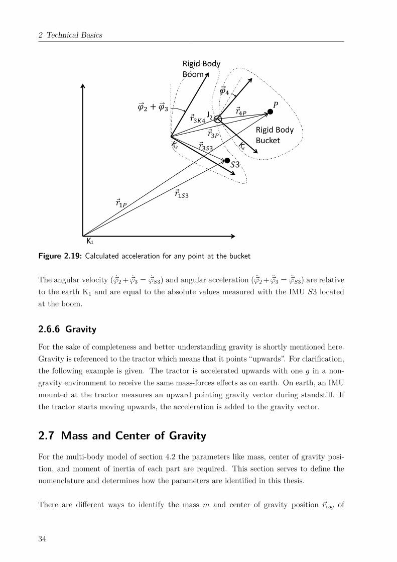
2 Technical Basics
K1
�
� �� + � �
� �
Rigid Body
Boom
Rigid Body
Bucket
J2 � �
Figure 2.19: Calculated acceleration for any point at the bucket
The angular velocity (~ϕ2 + ~ϕ3 = ~ϕS3) and angular acceleration (~ϕ2 + ~ϕ3 = ~ϕS3) are relative
to the earth K1 and are equal to the absolute values measured with the IMU S3 located
at the boom.
2.6.6 Gravity
For the sake of completeness and better understanding gravity is shortly mentioned here.
Gravity is referenced to the tractor which means that it points “upwards”. For clarification,
the following example is given. The tractor is accelerated upwards with one g in a non-
gravity environment to receive the same mass-forces effects as on earth. On earth, an IMU
mounted at the tractor measures an upward pointing gravity vector during standstill. If
the tractor starts moving upwards, the acceleration is added to the gravity vector.
2.7 Mass and Center of Gravity
For the multi-body model of section 4.2 the parameters like mass, center of gravity posi-
tion, and moment of inertia of each part are required. This section serves to define the
nomenclature and determines how the parameters are identified in this thesis.
There are different ways to identify the mass m and center of gravity position ~rcog of
34
2.7 Mass and Center of Gravity
a part. A part is defined as a rigid body with all stiff-mounted add-ons, such as brackets.
The boom-part, for instance, includes all hoses, fittings and pins. In order to not consider
a pin twice, it has to be determined to which part it belongs. One approach is to add a
density to 3D-CAD solids. This allows for the determination of the mass of a part and
its center of gravity position. If the part consists of several individual parts, the overall
mass has to be accumulated (∑
mi) and the overall center of gravity position is defined by
equation (2.25).
~rcog =
∑
mi~rcog_i∑
mi
(2.25)
All individual center of gravity positions ~rcog_i of each individual part need to be assigned
to the same coordinate system. This method is easy to accomplish with current CAD
systems but the effort increases with the amount of individual parts. The major difficulty
is to assign the appropriate density to each part. Also, deviations from the real part occur
due to manufacturing tolerances.
In this thesis is the mass of each front loader part measured with a scale in order to
avoid these deviations. The identification of the center of gravity is done as shown in
figure 2.20. Each part is hung up in different positions and the perpendicular is dropped
from the pivot point. The intersection of the perpendicular lines is the position of the
center of gravity 1. The front loader is assumed as symmetrical to the xz-plane. Hence,
the center of gravity position is only measured for x and z coordinates in the coordinate
system of the respective part. For instance, the vector ~rcogBM of the boom is referenced to
coordinate system K3. The mass and center of gravity position of each part of the front
loader are listed in the appendix in table A.2.
1A hydraulic cylinder consists of two parts, the cylinder and the rod. Appendix A.1 describes a procedureto define the center of gravity of both parts without disassembling the cylinder.
35
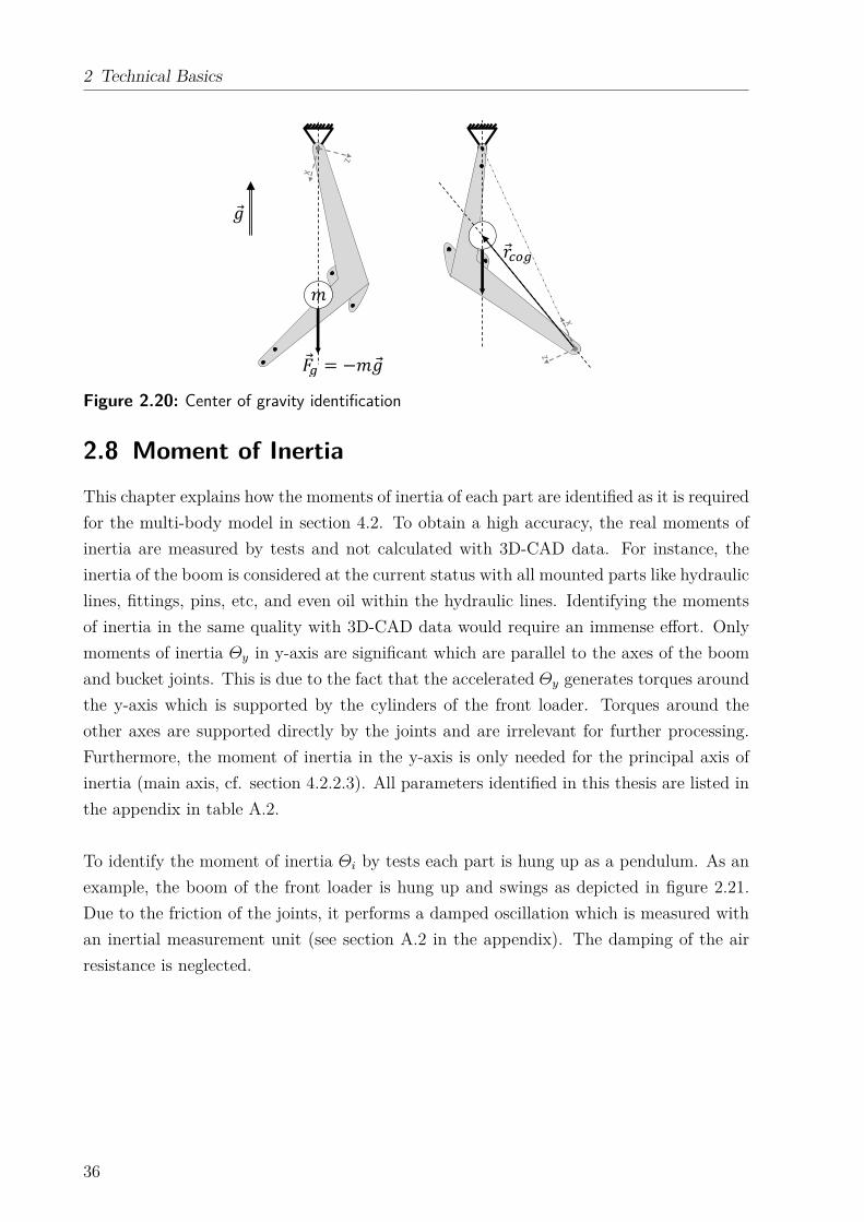
2 Technical Basics
� � �
� = − �Figure 2.20: Center of gravity identification
2.8 Moment of Inertia
This chapter explains how the moments of inertia of each part are identified as it is required
for the multi-body model in section 4.2. To obtain a high accuracy, the real moments of
inertia are measured by tests and not calculated with 3D-CAD data. For instance, the
inertia of the boom is considered at the current status with all mounted parts like hydraulic
lines, fittings, pins, etc, and even oil within the hydraulic lines. Identifying the moments
of inertia in the same quality with 3D-CAD data would require an immense effort. Only
moments of inertia Θy in y-axis are significant which are parallel to the axes of the boom
and bucket joints. This is due to the fact that the accelerated Θy generates torques around
the y-axis which is supported by the cylinders of the front loader. Torques around the
other axes are supported directly by the joints and are irrelevant for further processing.
Furthermore, the moment of inertia in the y-axis is only needed for the principal axis of
inertia (main axis, cf. section 4.2.2.3). All parameters identified in this thesis are listed in
the appendix in table A.2.
To identify the moment of inertia Θi by tests each part is hung up as a pendulum. As an
example, the boom of the front loader is hung up and swings as depicted in figure 2.21.
Due to the friction of the joints, it performs a damped oscillation which is measured with
an inertial measurement unit (see section A.2 in the appendix). The damping of the air
resistance is neglected.
36
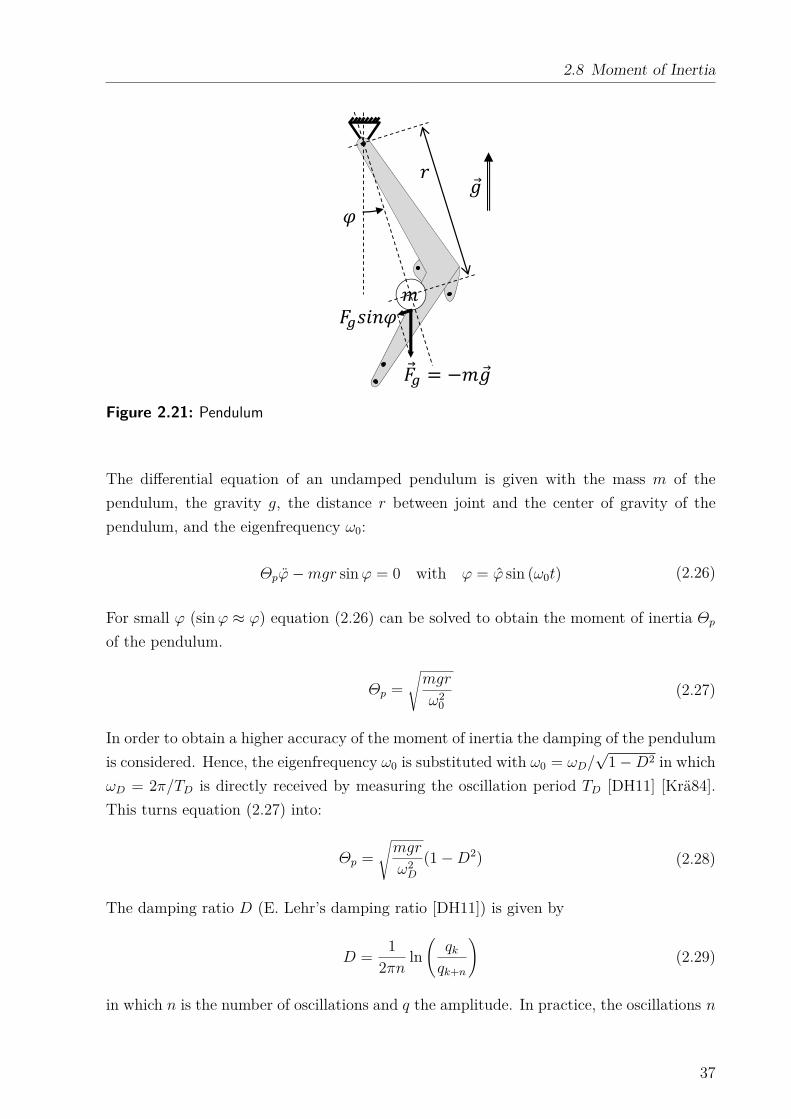
2.8 Moment of Inertia
� � �
� = − �� � �
Figure 2.21: Pendulum
The differential equation of an undamped pendulum is given with the mass m of the
pendulum, the gravity g, the distance r between joint and the center of gravity of the
pendulum, and the eigenfrequency ω0:
Θpϕ − mgr sin ϕ = 0 with ϕ = ϕ sin (ω0t) (2.26)
For small ϕ (sin ϕ ≈ ϕ) equation (2.26) can be solved to obtain the moment of inertia Θp
of the pendulum.
Θp =
√
mgr
ω20
(2.27)
In order to obtain a higher accuracy of the moment of inertia the damping of the pendulum
is considered. Hence, the eigenfrequency ω0 is substituted with ω0 = ωD/√
1 − D2 in which
ωD = 2π/TD is directly received by measuring the oscillation period TD [DH11] [Krä84].
This turns equation (2.27) into:
Θp =
√
mgr
ω2D
(1 − D2) (2.28)
The damping ratio D (E. Lehr’s damping ratio [DH11]) is given by
D =1
2πnln
(
qk
qk+n
)
(2.29)
in which n is the number of oscillations and q the amplitude. In practice, the oscillations n
37
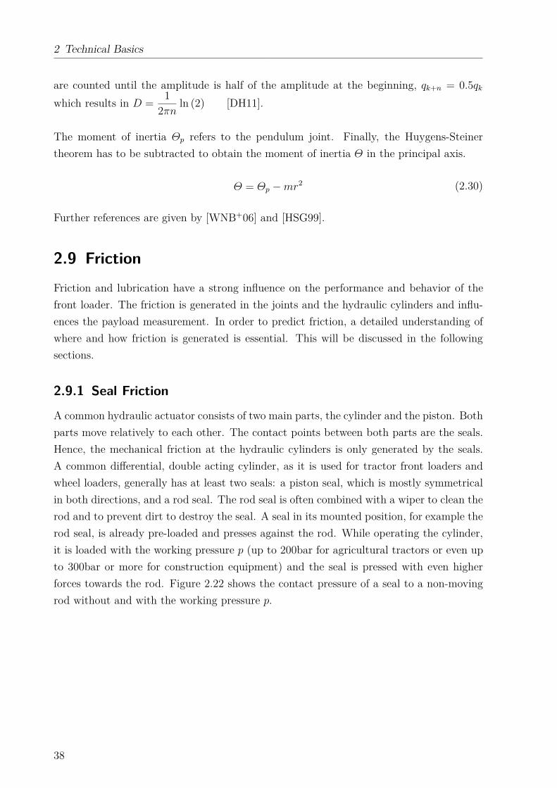
2 Technical Basics
are counted until the amplitude is half of the amplitude at the beginning, qk+n = 0.5qk
which results in D =1
2πnln (2) [DH11].
The moment of inertia Θp refers to the pendulum joint. Finally, the Huygens-Steiner
theorem has to be subtracted to obtain the moment of inertia Θ in the principal axis.
Θ = Θp − mr2 (2.30)
Further references are given by [WNB+06] and [HSG99].
2.9 Friction
Friction and lubrication have a strong influence on the performance and behavior of the
front loader. The friction is generated in the joints and the hydraulic cylinders and influ-
ences the payload measurement. In order to predict friction, a detailed understanding of
where and how friction is generated is essential. This will be discussed in the following
sections.
2.9.1 Seal Friction
A common hydraulic actuator consists of two main parts, the cylinder and the piston. Both
parts move relatively to each other. The contact points between both parts are the seals.
Hence, the mechanical friction at the hydraulic cylinders is only generated by the seals.
A common differential, double acting cylinder, as it is used for tractor front loaders and
wheel loaders, generally has at least two seals: a piston seal, which is mostly symmetrical
in both directions, and a rod seal. The rod seal is often combined with a wiper to clean the
rod and to prevent dirt to destroy the seal. A seal in its mounted position, for example the
rod seal, is already pre-loaded and presses against the rod. While operating the cylinder,
it is loaded with the working pressure p (up to 200bar for agricultural tractors or even up
to 300bar or more for construction equipment) and the seal is pressed with even higher
forces towards the rod. Figure 2.22 shows the contact pressure of a seal to a non-moving
rod without and with the working pressure p.
38
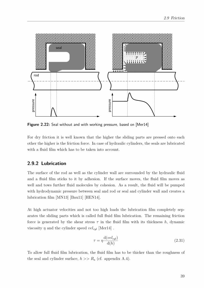
2.9 Friction
pre
ssu
re
pre
ssu
re
rod
seal
Figure 2.22: Seal without and with working pressure, based on [Mer14]
For dry friction it is well known that the higher the sliding parts are pressed onto each
other the higher is the friction force. In case of hydraulic cylinders, the seals are lubricated
with a fluid film which has to be taken into account.
2.9.2 Lubrication
The surface of the rod as well as the cylinder wall are surrounded by the hydraulic fluid
and a fluid film sticks to it by adhesion. If the surface moves, the fluid film moves as
well and tows further fluid molecules by cohesion. As a result, the fluid will be pumped
with hydrodynamic pressure between seal and rod or seal and cylinder wall and creates a
lubrication film [MN13] [Bau11] [HEN14].
At high actuator velocities and not too high loads the lubrication film completely sep-
arates the sliding parts which is called full fluid film lubrication. The remaining friction
force is generated by the shear stress τ in the fluid film with its thickness h, dynamic
viscosity η and the cylinder speed velcyl [Mer14] .
τ = ηd(velcyl)
d(h)(2.31)
To allow full fluid film lubrication, the fluid film has to be thicker than the roughness of
the seal and cylinder surface, h >> Ra (cf. appendix A.4).
39
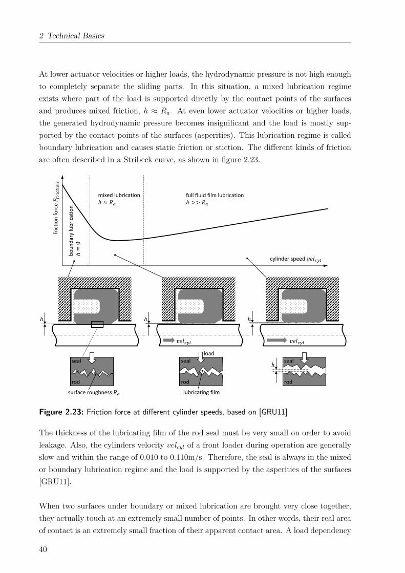
2 Technical Basics
At lower actuator velocities or higher loads, the hydrodynamic pressure is not high enough
to completely separate the sliding parts. In this situation, a mixed lubrication regime
exists where part of the load is supported directly by the contact points of the surfaces
and produces mixed friction, h ≈ Ra. At even lower actuator velocities or higher loads,
the generated hydrodynamic pressure becomes insignificant and the load is mostly sup-
ported by the contact points of the surfaces (asperities). This lubrication regime is called
boundary lubrication and causes static friction or stiction. The different kinds of friction
are often described in a Stribeck curve, as shown in figure 2.23.
ℎ��
rod
seal
lubricating film
ℎ��
rod
sealℎ
ℎ
rod
seal
surface roughness
load
bo
un
da
ry l
ub
rica
tio
n
ℎ=0
mixed lubricationℎ ≈ full fluid film lubricationℎ >>
cylinder speed ��
fric
tio
nfo
rce� ����
Figure 2.23: Friction force at different cylinder speeds, based on [GRU11]
The thickness of the lubricating film of the rod seal must be very small on order to avoid
leakage. Also, the cylinders velocity velcyl of a front loader during operation are generally
slow and within the range of 0.010 to 0.110m/s. Therefore, the seal is always in the mixed
or boundary lubrication regime and the load is supported by the asperities of the surfaces
[GRU11].
When two surfaces under boundary or mixed lubrication are brought very close together,
they actually touch at an extremely small number of points. In other words, their real area
of contact is an extremely small fraction of their apparent contact area. A load dependency
40
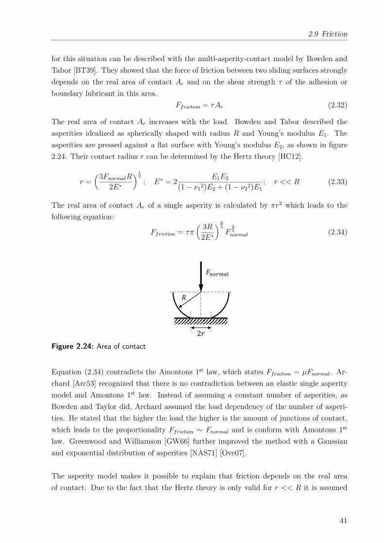
2.9 Friction
for this situation can be described with the multi-asperity-contact model by Bowden and
Tabor [BT39]. They showed that the force of friction between two sliding surfaces strongly
depends on the real area of contact Ar and on the shear strength τ of the adhesion or
boundary lubricant in this area.
Ffriction = τAr (2.32)
The real area of contact Ar increases with the load. Bowden and Tabor described the
asperities idealized as spherically shaped with radius R and Young’s modulus E1. The
asperities are pressed against a flat surface with Young’s modulus E2, as shown in figure
2.24. Their contact radius r can be determined by the Hertz theory [HC12].
r =(
3FnormalR
2E∗
)
1
3
; E∗ = 2E1E2
(1 − ν12)E2 + (1 − ν2
2)E1
; r << R (2.33)
The real area of contact Ar of a single asperity is calculated by πr2 which leads to the
following equation:
Ffriction = τπ(
3R
2E∗
)
2
3
F2
3
normal (2.34)
� ��
2�Figure 2.24: Area of contact
Equation (2.34) contradicts the Amontons 1st law, which states Ffriction = µFnormal. Ar-
chard [Arc53] recognized that there is no contradiction between an elastic single asperity
model and Amontons 1st law. Instead of assuming a constant number of asperities, as
Bowden and Taylor did, Archard assumed the load dependency of the number of asperi-
ties. He stated that the higher the load the higher is the amount of junctions of contact,
which leads to the proportionality Ffriction ∼ Fnormal and is conform with Amontons 1st
law. Greenwood and Williamson [GW66] further improved the method with a Gaussian
and exponential distribution of asperities [NAS71] [Ove07].
The asperity model makes it possible to explain that friction depends on the real area
of contact. Due to the fact that the Hertz theory is only valid for r << R it is assumed
41
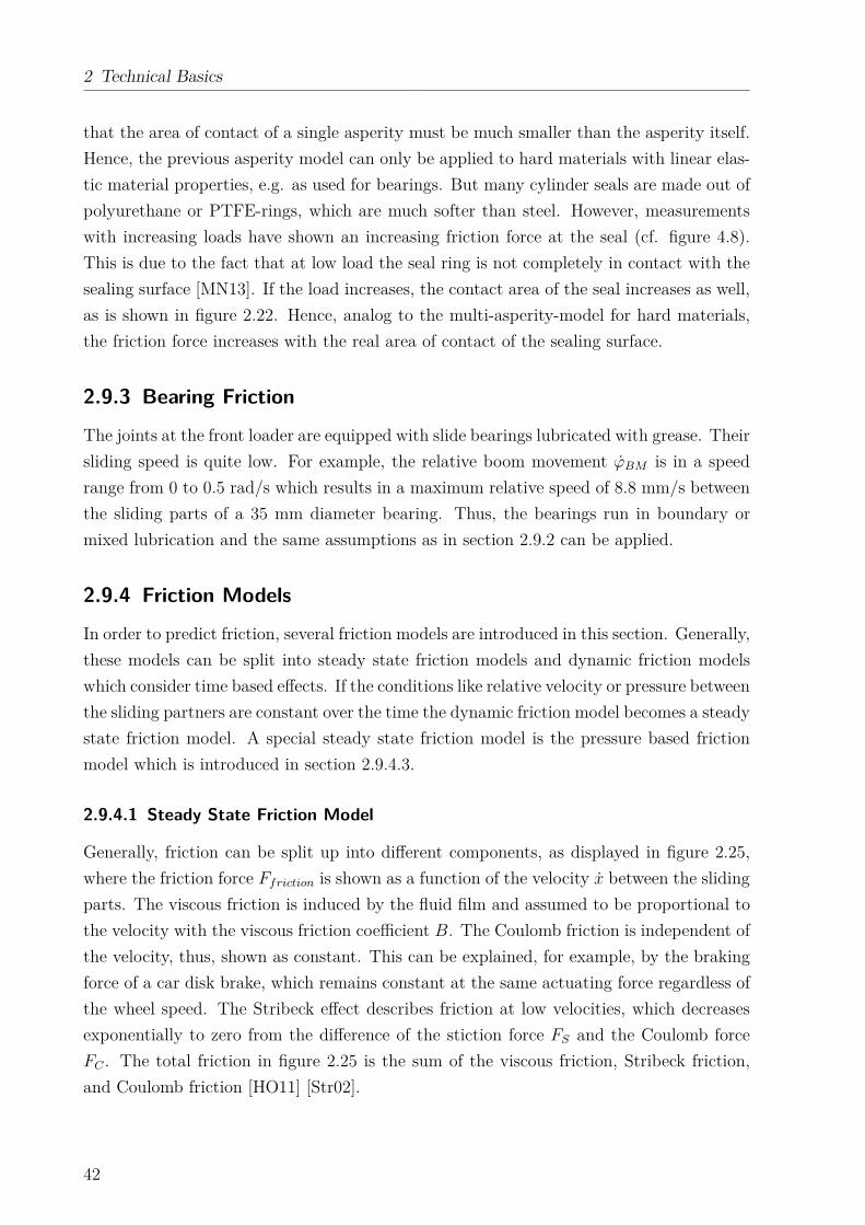
2 Technical Basics
that the area of contact of a single asperity must be much smaller than the asperity itself.
Hence, the previous asperity model can only be applied to hard materials with linear elas-
tic material properties, e.g. as used for bearings. But many cylinder seals are made out of
polyurethane or PTFE-rings, which are much softer than steel. However, measurements
with increasing loads have shown an increasing friction force at the seal (cf. figure 4.8).
This is due to the fact that at low load the seal ring is not completely in contact with the
sealing surface [MN13]. If the load increases, the contact area of the seal increases as well,
as is shown in figure 2.22. Hence, analog to the multi-asperity-model for hard materials,
the friction force increases with the real area of contact of the sealing surface.
2.9.3 Bearing Friction
The joints at the front loader are equipped with slide bearings lubricated with grease. Their
sliding speed is quite low. For example, the relative boom movement ϕBM is in a speed
range from 0 to 0.5 rad/s which results in a maximum relative speed of 8.8 mm/s between
the sliding parts of a 35 mm diameter bearing. Thus, the bearings run in boundary or
mixed lubrication and the same assumptions as in section 2.9.2 can be applied.
2.9.4 Friction Models
In order to predict friction, several friction models are introduced in this section. Generally,
these models can be split into steady state friction models and dynamic friction models
which consider time based effects. If the conditions like relative velocity or pressure between
the sliding partners are constant over the time the dynamic friction model becomes a steady
state friction model. A special steady state friction model is the pressure based friction
model which is introduced in section 2.9.4.3.
2.9.4.1 Steady State Friction Model
Generally, friction can be split up into different components, as displayed in figure 2.25,
where the friction force Ffriction is shown as a function of the velocity x between the sliding
parts. The viscous friction is induced by the fluid film and assumed to be proportional to
the velocity with the viscous friction coefficient B. The Coulomb friction is independent of
the velocity, thus, shown as constant. This can be explained, for example, by the braking
force of a car disk brake, which remains constant at the same actuating force regardless of
the wheel speed. The Stribeck effect describes friction at low velocities, which decreases
exponentially to zero from the difference of the stiction force FS and the Coulomb force
FC . The total friction in figure 2.25 is the sum of the viscous friction, Stribeck friction,
and Coulomb friction [HO11] [Str02].
42
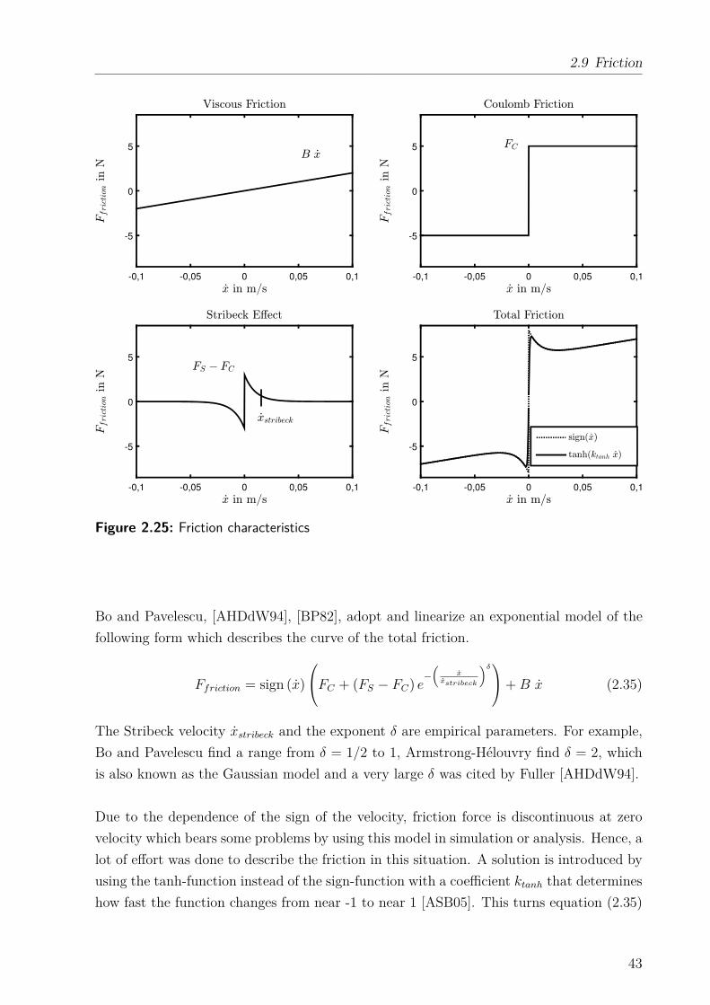
2.9 Friction
-0,1 -0,05 0 0,05 0,1
-5
0
5
-0,1 -0,05 0 0,05 0,1
-5
0
5
-0,1 -0,05 0 0,05 0,1
-5
0
5
-0,1 -0,05 0 0,05 0,1
-5
0
5
Figure 2.25: Friction characteristics
Bo and Pavelescu, [AHDdW94], [BP82], adopt and linearize an exponential model of the
following form which describes the curve of the total friction.
Ffriction = sign (x)
FC + (FS − FC) e−
(
xxstribeck
)δ
+ B x (2.35)
The Stribeck velocity xstribeck and the exponent δ are empirical parameters. For example,
Bo and Pavelescu find a range from δ = 1/2 to 1, Armstrong-Hélouvry find δ = 2, which
is also known as the Gaussian model and a very large δ was cited by Fuller [AHDdW94].
Due to the dependence of the sign of the velocity, friction force is discontinuous at zero
velocity which bears some problems by using this model in simulation or analysis. Hence, a
lot of effort was done to describe the friction in this situation. A solution is introduced by
using the tanh-function instead of the sign-function with a coefficient ktanh that determines
how fast the function changes from near -1 to near 1 [ASB05]. This turns equation (2.35)
43
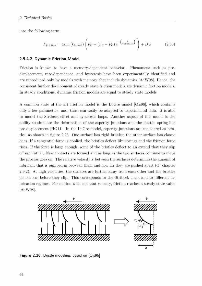
2 Technical Basics
into the following term:
Ffriction = tanh (ktanhx)
FC + (FS − FC) e−
(
xxstribeck
)δ
+ B x (2.36)
2.9.4.2 Dynamic Friction Model
Friction is known to have a memory-dependent behavior. Phenomena such as pre-
displacement, rate-dependence, and hysteresis have been experimentally identified and
are reproduced only by models with memory that include dynamics [AdW08]. Hence, the
consistent further development of steady state friction models are dynamic friction models.
In steady conditions, dynamic friction models are equal to steady state models.
A common state of the art friction model is the LuGre model [Ols96], which contains
only a few parameters, and, thus, can easily be adapted to experimental data. It is able
to model the Stribeck effect and hysteresis loops. Another aspect of this model is the
ability to simulate the deformation of the asperity junctions and the elastic, spring-like
pre-displacement [HO11]. In the LuGre model, asperity junctions are considered as bris-
tles, as shown in figure 2.26. One surface has rigid bristles; the other surface has elastic
ones. If a tangential force is applied, the bristles deflect like springs and the friction force
rises. If the force is large enough, some of the bristles deflect to an extend that they slip
off each other. New contacts are formed and as long as the two surfaces continue to move
the process goes on. The relative velocity x between the surfaces determines the amount of
lubricant that is pumped in between them and how far they are pushed apart (cf. chapter
2.9.2). At high velocities, the surfaces are further away from each other and the bristles
deflect less before they slip. This corresponds to the Stribeck effect and to different lu-
brication regimes. For motion with constant velocity, friction reaches a steady state value
[AdW08]. �
�
���0
Figure 2.26: Bristle modeling, based on [Ols96]
44
2.9 Friction
The LuGre model is based on a single bristle which represents the average behavior and
which can never slip off. The parameter σ0 is the average stiffness of the bristles; the
parameter σ1 is the micro-viscous coefficient which is equivalent to a damping coefficient.
The friction force is described in equation (2.37) with the viscous friction term Bx.
Ffriction = σ0z + σ1z + Bx (2.37)
The deflection of the elastic bristle is denoted by z and modeled by the following equation.
z = x − |x|g(x)
z (2.38)
The function g(x) is described as follows.
g(x) =1
σ0
FC + (FS − FC) e−
(
xxstribeck
)δ
(2.39)
The steady state friction force Ffriction,ss arises when the velocity x is held constant. Thus,
the deflection rate will be zero z = 0 and the steady state deflection zss is described by
the following equation:
zss =x
|x|g(x) = sign (x)g(x) (2.40)
This turns equation (2.37) into the following term which is equal to equation (2.35) of the
steady state friction model.
Ffriction,ss = σ0zss + Bx
= σ0 sign (x)g(x) + Bx
= sign (x)
FC + (FS − FC) e−
(
xxstribeck
)δ
+ Bx
(2.41)
In conclusion, the dynamic friction models such as the LuGre are able to model phenomena
like pre-displacement, rate-dependence, and hysteresis. In steady state conditions, they
are equal to a steady state model. In real time applications it must be mentioned that, a
high sample rate is needed to run a dynamic friction model on a controller, which is due
to the fast transient response of pre-displacement.
2.9.4.3 Pressure Based Model
The pressure based friction model is a steady state friction model especially developed for
hydraulic applications. It is also possible to combine the pressure based friction model with
the previously described friction models, for instance, by replacing the Coulomb friction.
45
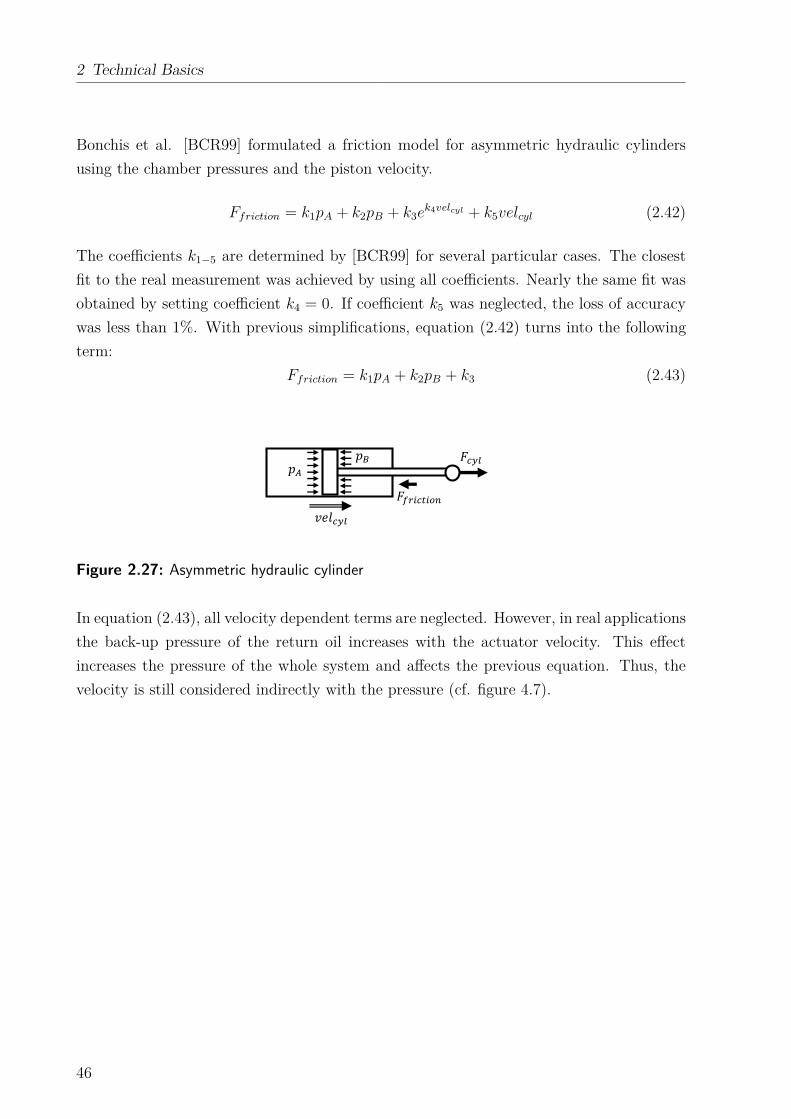
2 Technical Basics
Bonchis et al. [BCR99] formulated a friction model for asymmetric hydraulic cylinders
using the chamber pressures and the piston velocity.
Ffriction = k1pA + k2pB + k3ek4velcyl + k5velcyl (2.42)
The coefficients k1−5 are determined by [BCR99] for several particular cases. The closest
fit to the real measurement was achieved by using all coefficients. Nearly the same fit was
obtained by setting coefficient k4 = 0. If coefficient k5 was neglected, the loss of accuracy
was less than 1%. With previous simplifications, equation (2.42) turns into the following
term:
Ffriction = k1pA + k2pB + k3 (2.43)
���
�� �� ��
Figure 2.27: Asymmetric hydraulic cylinder
In equation (2.43), all velocity dependent terms are neglected. However, in real applications
the back-up pressure of the return oil increases with the actuator velocity. This effect
increases the pressure of the whole system and affects the previous equation. Thus, the
velocity is still considered indirectly with the pressure (cf. figure 4.7).
46
3 Position Detection
The angular position of the front loader is required to calculate the vectors which are used
in the subsequently discussed weighing algorithm of chapter 4. There are several ways to
detect the position of the front loader relative to the machine, for instance, by measuring
the actuator length with stroke sensors or by detecting the boom and bucket angle with
rotary sensors. The implementation of the position detection is irrelevant for the weighing
algorithm, hence, the position detection is discussed separately in this chapter.
This thesis pursues an approach that uses inertial measurement units (IMUs), also known
as acceleration sensors combined with gyros, to detect the position of the front loader. The
IMUs’ advantages are that they consist of non-moving parts and that they can be mounted
individually in a protected position at boom, bucket, or tool carrier. For this purpose, the
position of the front loader relative to the tractor is defined by the angle ϕBM between
boom and tractor chassis and by the angle ϕBU between bucket or tool carrier and tractor
chassis. Thus, the angle ϕBM is equal to the rotation angle ϕ3y between the coordinate
system K2 and K3 (cf. figure 2.18). The angle ϕBU = ϕ3y + ϕ4y is the rotation of the co-
ordinate system K4 relative to K2. With the knowledge of these angles, all other variables
such as the cylinder strokes can be derived. To receive these angles, the accelerations at
the chassis, boom, and bucket are measured and compared to each other. Therefore, the
front loader is equipped with three IMUs (cf. section A.3.3).
• The IMU S2 is mounted to the chassis and assigned to the tractor coordinate
system K2.
• The IMU S3 is mounted to the boom and assigned to the boom coordinate system K3.
• The IMU S4 is mounted to the bucket or tool carrier and assigned to the bucket
coordinate system K4.
3.1 Angle between Chassis and Boom
To determine the angle ϕBM , the acceleration vector ~aS3 = ~rS3 is measured in the boom
coordinate system K3 using IMU S3. At the same time, the acceleration vector ~aS2 = ~rS2
is measured in the chassis coordinate system K2 using IMU S2. In a next step, the
acceleration vector ~aS2 = ~rS2 is calculated for the IMU position of S3 using equation (2.22),
which results in ~aS3byS2 of equation (3.1). Equation (3.1) includes ~r2K3 = ~0, the angular
47
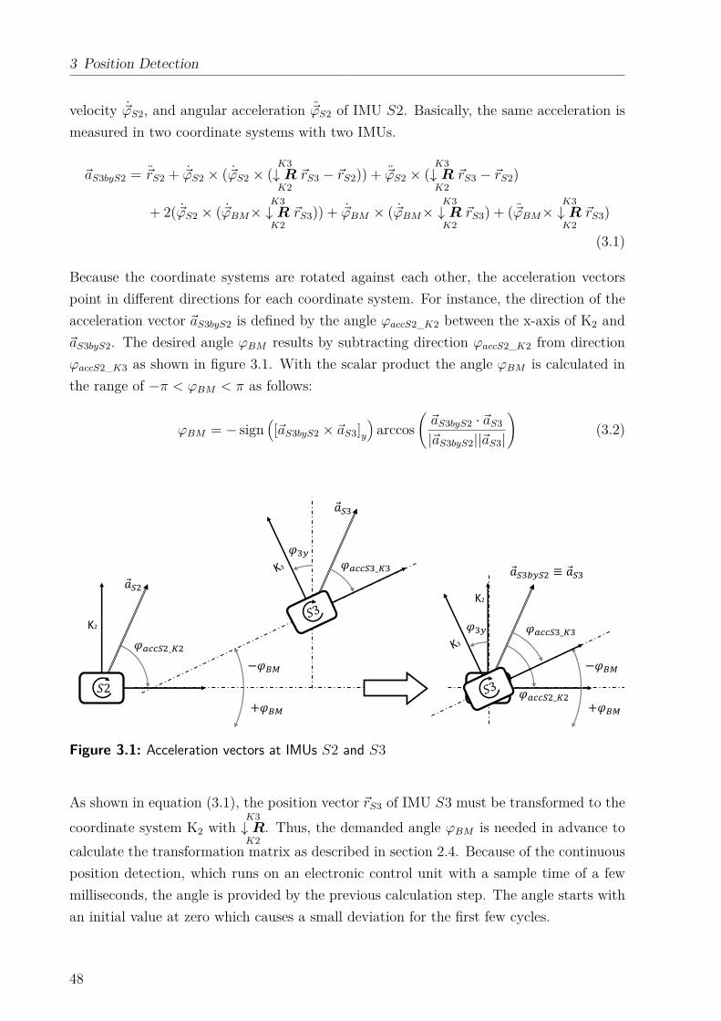
3 Position Detection
velocity ~ϕS2, and angular acceleration ~ϕS2 of IMU S2. Basically, the same acceleration is
measured in two coordinate systems with two IMUs.
~aS3byS2 = ~rS2 + ~ϕS2 × ( ~ϕS2 × (K3
↓ RK2
~rS3 − ~rS2)) + ~ϕS2 × (K3
↓ RK2
~rS3 − ~rS2)
+ 2( ~ϕS2 × ( ~ϕBM×K3
↓ RK2
~rS3)) + ~ϕBM × ( ~ϕBM×K3
↓ RK2
~rS3) + ( ~ϕBM×K3
↓ RK2
~rS3)
(3.1)
Because the coordinate systems are rotated against each other, the acceleration vectors
point in different directions for each coordinate system. For instance, the direction of the
acceleration vector ~aS3byS2 is defined by the angle ϕaccS2_K2 between the x-axis of K2 and
~aS3byS2. The desired angle ϕBM results by subtracting direction ϕaccS2_K2 from direction
ϕaccS2_K3 as shown in figure 3.1. With the scalar product the angle ϕBM is calculated in
the range of −π < ϕBM < π as follows:
ϕBM = − sign(
[~aS3byS2 × ~aS3]y)
arccos
(
~aS3byS2 · ~aS3
|~aS3byS2||~aS3|
)
(3.2)
K2
� ≡ �
� _�
−���
+���
2
� _� � K2
�
� _� −���
+���
2
�
� _�
�
Figure 3.1: Acceleration vectors at IMUs S2 and S3
As shown in equation (3.1), the position vector ~rS3 of IMU S3 must be transformed to the
coordinate system K2 withK3
↓ RK2
. Thus, the demanded angle ϕBM is needed in advance to
calculate the transformation matrix as described in section 2.4. Because of the continuous
position detection, which runs on an electronic control unit with a sample time of a few
milliseconds, the angle is provided by the previous calculation step. The angle starts with
an initial value at zero which causes a small deviation for the first few cycles.
48
3.2 Angle between Chassis and Bucket
3.2 Angle between Chassis and Bucket
The angle ϕBU between chassis and boom is calculated in the same way as ϕBM in the
previous chapter 3.1 but with the acceleration vectors of S3 and S4 and equation (2.24)
(cf. equation (4.24)). The angle ϕBU is a sum of the angle ϕBM and the angle ϕ4y between
boom and bucket, ϕBU = ϕBM + ϕ4y.
It is also possible to calculate ϕBU directly by using the acceleration vectors of S2 and S4
and equation (2.23). In this case, there will be a higher deviation due to one additional
joint between the IMUs which performs relative movements. In addition, a longer distance
between the two IMUs causes a higher influence on ϕBU because of a noise corrupted an-
gular velocity and acceleration signal (cf. equation (2.23) and equation (2.24), distance
(~r2K3 + ~r3K4 + ~r4P − ~r2S2) vs. (~r3K4 + ~r4P − ~r3S3) ).
3.3 Interchangeability and Sensor Configuration
It is irrelevant whether the accelerations are calculated at the IMU position of S3 as in
section 3.1 or vice versa at the IMU position of S2. With both methods, it is possible
to obtain the angle. In order to transfer a measured acceleration to another position us-
ing equation (2.22), the angular velocities and angular accelerations have to be measured.
Hence, it is obvious to mount an inertial measurement unit S3 to the boom that provides
accelerations, angular velocity and derived angular acceleration for all axis. With these
signals, the accelerations at the IMU positions S2 and S4 of chassis and bucket can be
calculated. In this case, it is sufficient if IMUs S2 and S4 provide accelerations for all axis
and angular velocity and acceleration only around the y-axis. Furthermore, the acceler-
ations, angular velocities, and angular accelerations for all axis of the boom IMU S3 are
needed for the dynamic weighing in chapter 4.
3.4 Continuous Angle Function
A continuous position angle is needed for further calculations. Depending on the kinemat-
ics and the coordinate systems of the front loader the measured position angle ϕBM or
ϕBU overshoot π and the angle is a discontinuous function and jumps to −π.
To prevent the angle to switch from +π to −π, a start angle ϕstart is defined, which
is outside of the movement range. For example, if ϕstart is larger than −π but the output
of equation (3.2) is smaller than ϕstart, the value of 2π has to be added, as shown in figure
3.2. Thus, the angle is continuous in the range from ϕstart to ϕstart + 2π.
49
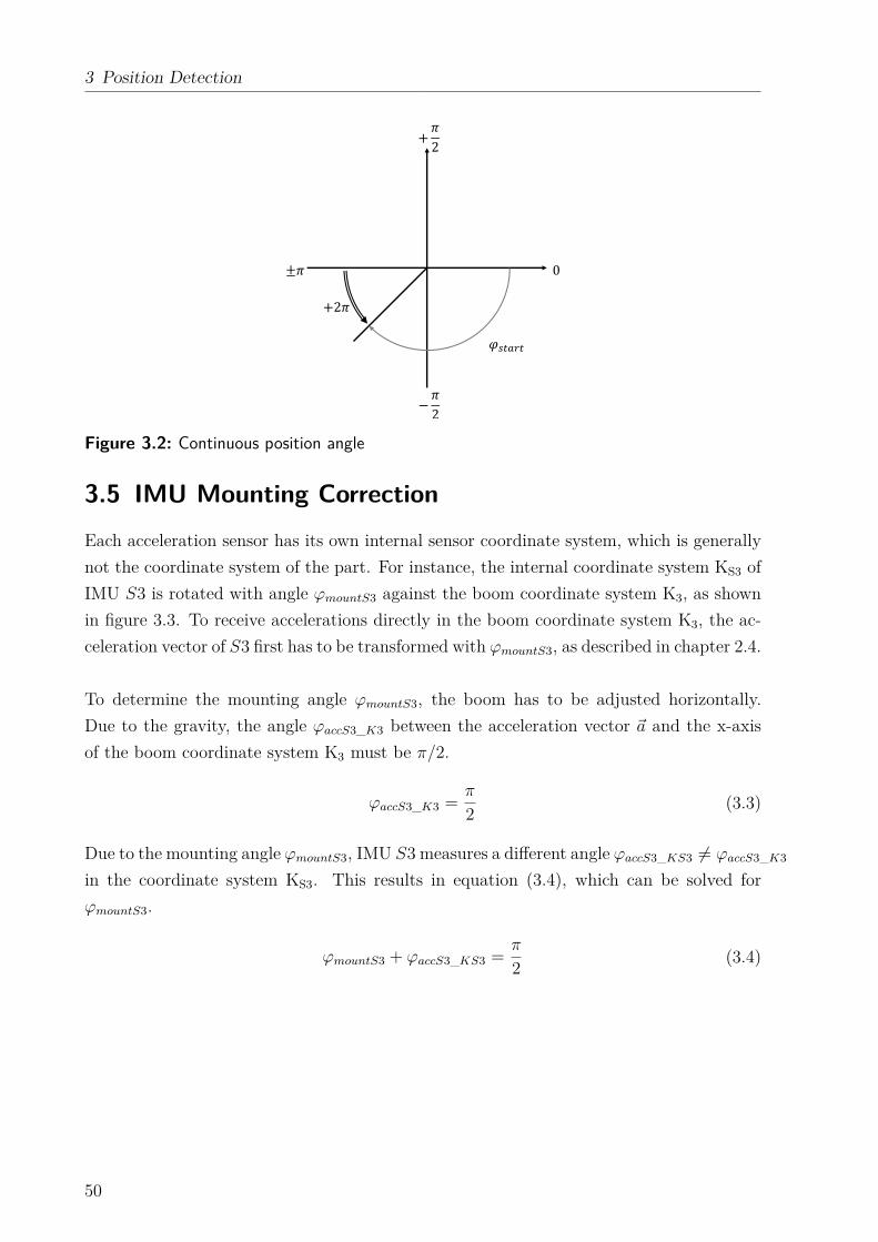
3 Position Detection
0
+�2
−�2
±�
� �
+2�
Figure 3.2: Continuous position angle
3.5 IMU Mounting Correction
Each acceleration sensor has its own internal sensor coordinate system, which is generally
not the coordinate system of the part. For instance, the internal coordinate system KS3 of
IMU S3 is rotated with angle ϕmountS3 against the boom coordinate system K3, as shown
in figure 3.3. To receive accelerations directly in the boom coordinate system K3, the ac-
celeration vector of S3 first has to be transformed with ϕmountS3, as described in chapter 2.4.
To determine the mounting angle ϕmountS3, the boom has to be adjusted horizontally.
Due to the gravity, the angle ϕaccS3_K3 between the acceleration vector ~a and the x-axis
of the boom coordinate system K3 must be π/2.
ϕaccS3_K3 =π
2(3.3)
Due to the mounting angle ϕmountS3, IMU S3 measures a different angle ϕaccS3_KS3 6= ϕaccS3_K3
in the coordinate system KS3. This results in equation (3.4), which can be solved for
ϕmountS3.
ϕmountS3 + ϕaccS3_KS3 =π
2(3.4)
50
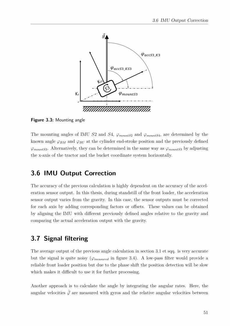
3.6 IMU Output Correction
K3
� � _�
� �
� _�
Figure 3.3: Mounting angle
The mounting angles of IMU S2 and S4, ϕmountS2 and ϕmountS4, are determined by the
known angle ϕBM and ϕBU at the cylinder end-stroke position and the previously defined
ϕmountS3. Alternatively, they can be determined in the same way as ϕmountS3 by adjusting
the x-axis of the tractor and the bucket coordinate system horizontally.
3.6 IMU Output Correction
The accuracy of the previous calculation is highly dependent on the accuracy of the accel-
eration sensor output. In this thesis, during standstill of the front loader, the acceleration
sensor output varies from the gravity. In this case, the sensor outputs must be corrected
for each axis by adding corresponding factors or offsets. These values can be obtained
by aligning the IMU with different previously defined angles relative to the gravity and
comparing the actual acceleration output with the gravity.
3.7 Signal filtering
The average output of the previous angle calculation in section 3.1 et sqq. is very accurate
but the signal is quite noisy (ϕmeasured in figure 3.4). A low-pass filter would provide a
reliable front loader position but due to the phase shift the position detection will be slow
which makes it difficult to use it for further processing.
Another approach is to calculate the angle by integrating the angular rates. Here, the
angular velocities ~ϕ are measured with gyros and the relative angular velocities between
51
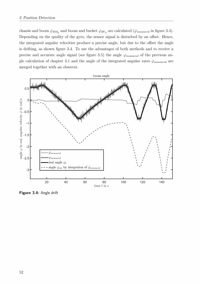
3 Position Detection
chassis and boom ϕBMyand boom and bucket ϕBUy
are calculated (ϕmeasured in figure 3.4).
Depending on the quality of the gyro, the sensor signal is disturbed by an offset. Hence,
the integrated angular velocities produce a precise angle, but due to the offset the angle
is drifting, as shown figure 3.4. To use the advantages of both methods and to receive a
precise and accurate angle signal (see figure 3.5) the angle ϕmeasured of the previous an-
gle calculation of chapter 3.1 and the angle of the integrated angular rates ϕmeasured are
merged together with an observer.
20 40 60 80 100 120 140
-3
-2.5
-2
-1.5
-1
-0.5
0
0.5
Figure 3.4: Angle drift
52
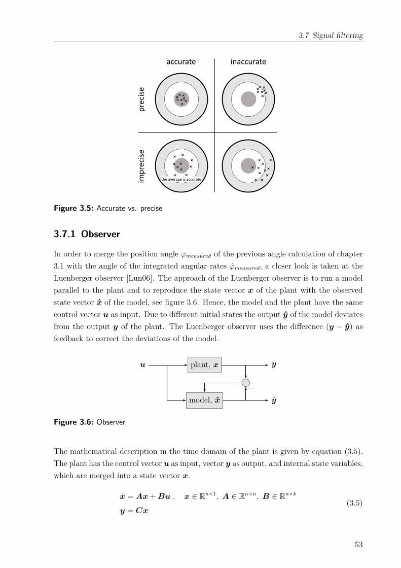
3.7 Signal filtering
accurate inaccurate
pre
cise
imp
reci
se
the average is accurate
Figure 3.5: Accurate vs. precise
3.7.1 Observer
In order to merge the position angle ϕmeasured of the previous angle calculation of chapter
3.1 with the angle of the integrated angular rates ϕmeasured, a closer look is taken at the
Luenberger observer [Lun06]. The approach of the Luenberger observer is to run a model
parallel to the plant and to reproduce the state vector x of the plant with the observed
state vector x of the model, see figure 3.6. Hence, the model and the plant have the same
control vector u as input. Due to different initial states the output y of the model deviates
from the output y of the plant. The Luenberger observer uses the difference (y − y) as
feedback to correct the deviations of the model.
u plant, x y
model, x y
−
Figure 3.6: Observer
The mathematical description in the time domain of the plant is given by equation (3.5).
The plant has the control vector u as input, vector y as output, and internal state variables,
which are merged into a state vector x.
x = Ax + Bu , x ∈ Rn×1, A ∈ R
n×n, B ∈ Rn×k
y = Cx(3.5)
53
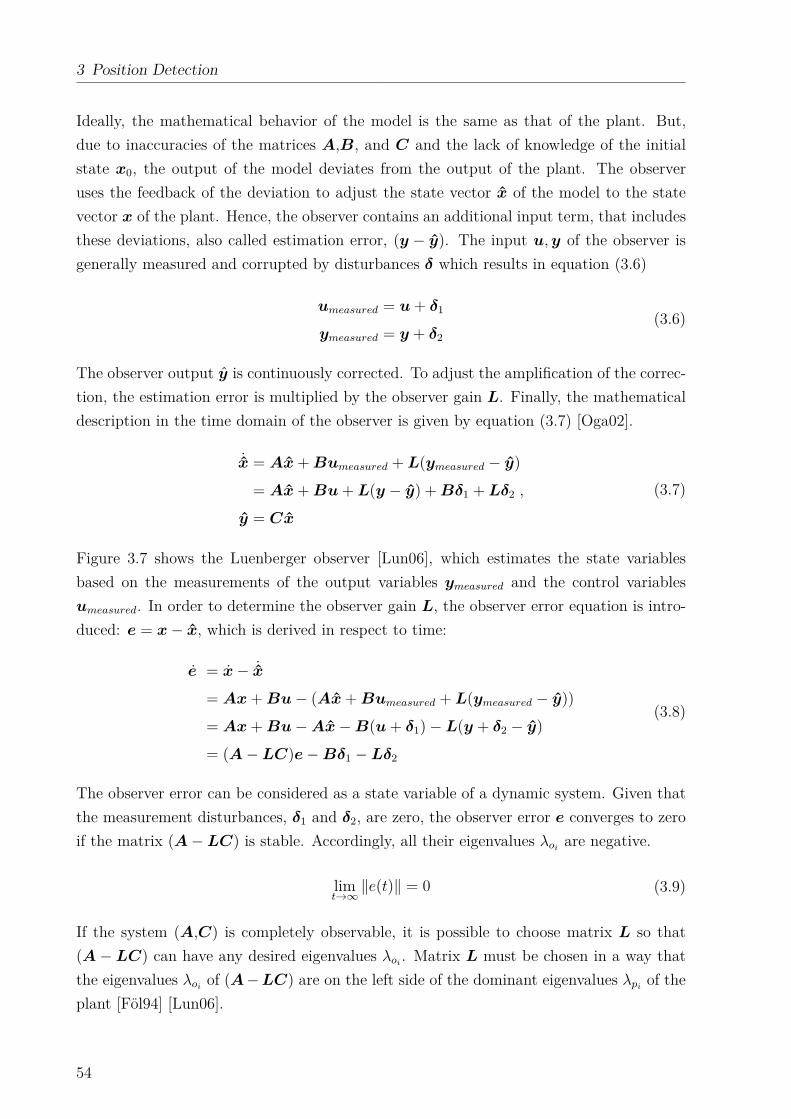
3 Position Detection
Ideally, the mathematical behavior of the model is the same as that of the plant. But,
due to inaccuracies of the matrices A,B, and C and the lack of knowledge of the initial
state x0, the output of the model deviates from the output of the plant. The observer
uses the feedback of the deviation to adjust the state vector x of the model to the state
vector x of the plant. Hence, the observer contains an additional input term, that includes
these deviations, also called estimation error, (y − y). The input u, y of the observer is
generally measured and corrupted by disturbances δ which results in equation (3.6)
umeasured = u + δ1
ymeasured = y + δ2
(3.6)
The observer output y is continuously corrected. To adjust the amplification of the correc-
tion, the estimation error is multiplied by the observer gain L. Finally, the mathematical
description in the time domain of the observer is given by equation (3.7) [Oga02].
˙x = Ax + Bumeasured + L(ymeasured − y)
= Ax + Bu + L(y − y) + Bδ1 + Lδ2 ,
y = Cx
(3.7)
Figure 3.7 shows the Luenberger observer [Lun06], which estimates the state variables
based on the measurements of the output variables ymeasured and the control variables
umeasured. In order to determine the observer gain L, the observer error equation is intro-
duced: e = x − x, which is derived in respect to time:
e = x − ˙x
= Ax + Bu − (Ax + Bumeasured + L(ymeasured − y))
= Ax + Bu − Ax − B(u + δ1) − L(y + δ2 − y)
= (A − LC)e − Bδ1 − Lδ2
(3.8)
The observer error can be considered as a state variable of a dynamic system. Given that
the measurement disturbances, δ1 and δ2, are zero, the observer error e converges to zero
if the matrix (A − LC) is stable. Accordingly, all their eigenvalues λoiare negative.
limt→∞
‖e(t)‖ = 0 (3.9)
If the system (A,C) is completely observable, it is possible to choose matrix L so that
(A − LC) can have any desired eigenvalues λoi. Matrix L must be chosen in a way that
the eigenvalues λoiof (A − LC) are on the left side of the dominant eigenvalues λpi
of the
plant [Föl94] [Lun06].
54
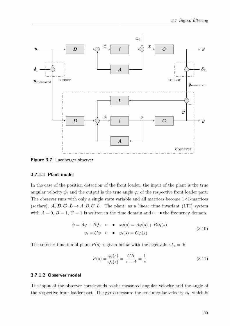
3.7 Signal filtering
u B∫
C y
δ1 A δ2
L
B∫
C y
A
x0
x x
ymeasured
−y
umeasured
˙x x
sensor sensor
observer
Figure 3.7: Luenberger observer
3.7.1.1 Plant model
In the case of the position detection of the front loader, the input of the plant is the true
angular velocity ϕt and the output is the true angle ϕt of the respective front loader part.
The observer runs with only a single state variable and all matrices become 1×1-matrices
(scalars), A, B, C, L → A, B, C, L. The plant, as a linear time invariant (LTI) system
with A = 0, B = 1, C = 1 is written in the time domain and ❞ tthe frequency domain.
ϕ = Aϕ + Bϕt❞ t sϕ(s) = Aϕ(s) + Bϕt(s)
ϕt = Cϕ ❞ t ϕt(s) = Cϕ(s)(3.10)
The transfer function of plant P (s) is given below with the eigenvalue λp = 0:
P (s) =ϕt(s)
ϕt(s)=
CB
s − A=
1
s(3.11)
3.7.1.2 Observer model
The input of the observer corresponds to the measured angular velocity and the angle of
the respective front loader part. The gyros measure the true angular velocity ϕt, which is
55
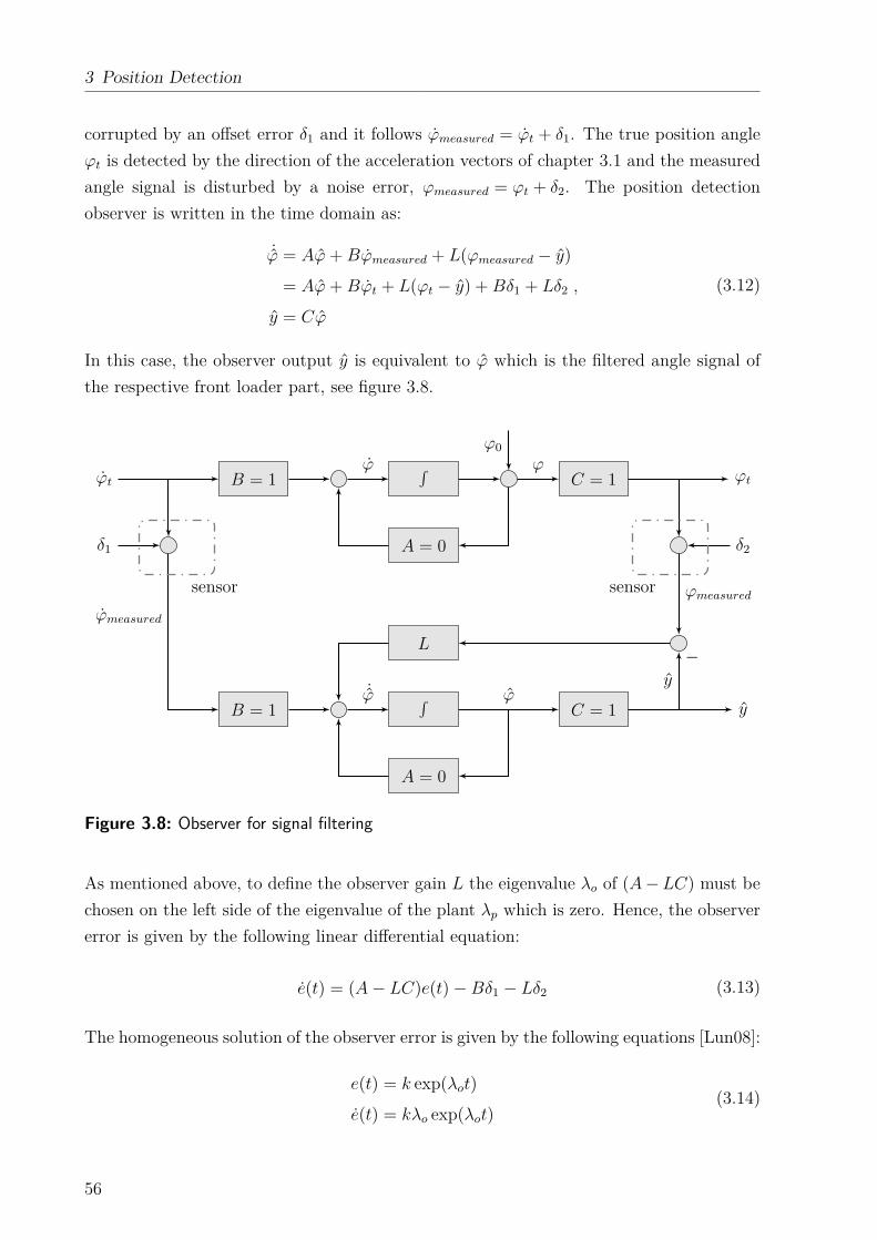
3 Position Detection
corrupted by an offset error δ1 and it follows ϕmeasured = ϕt + δ1. The true position angle
ϕt is detected by the direction of the acceleration vectors of chapter 3.1 and the measured
angle signal is disturbed by a noise error, ϕmeasured = ϕt + δ2. The position detection
observer is written in the time domain as:
˙ϕ = Aϕ + Bϕmeasured + L(ϕmeasured − y)
= Aϕ + Bϕt + L(ϕt − y) + Bδ1 + Lδ2 ,
y = Cϕ
(3.12)
In this case, the observer output y is equivalent to ϕ which is the filtered angle signal of
the respective front loader part, see figure 3.8.
ϕt B = 1∫
C = 1 ϕt
δ1 A = 0 δ2
L
B = 1∫
C = 1 y
A = 0
ϕ0
ϕ ϕ
ϕmeasured
−y
ϕmeasured
˙ϕ ϕ
sensor sensor
Figure 3.8: Observer for signal filtering
As mentioned above, to define the observer gain L the eigenvalue λo of (A − LC) must be
chosen on the left side of the eigenvalue of the plant λp which is zero. Hence, the observer
error is given by the following linear differential equation:
e(t) = (A − LC)e(t) − Bδ1 − Lδ2 (3.13)
The homogeneous solution of the observer error is given by the following equations [Lun08]:
e(t) = k exp(λot)
e(t) = kλo exp(λot)(3.14)
56
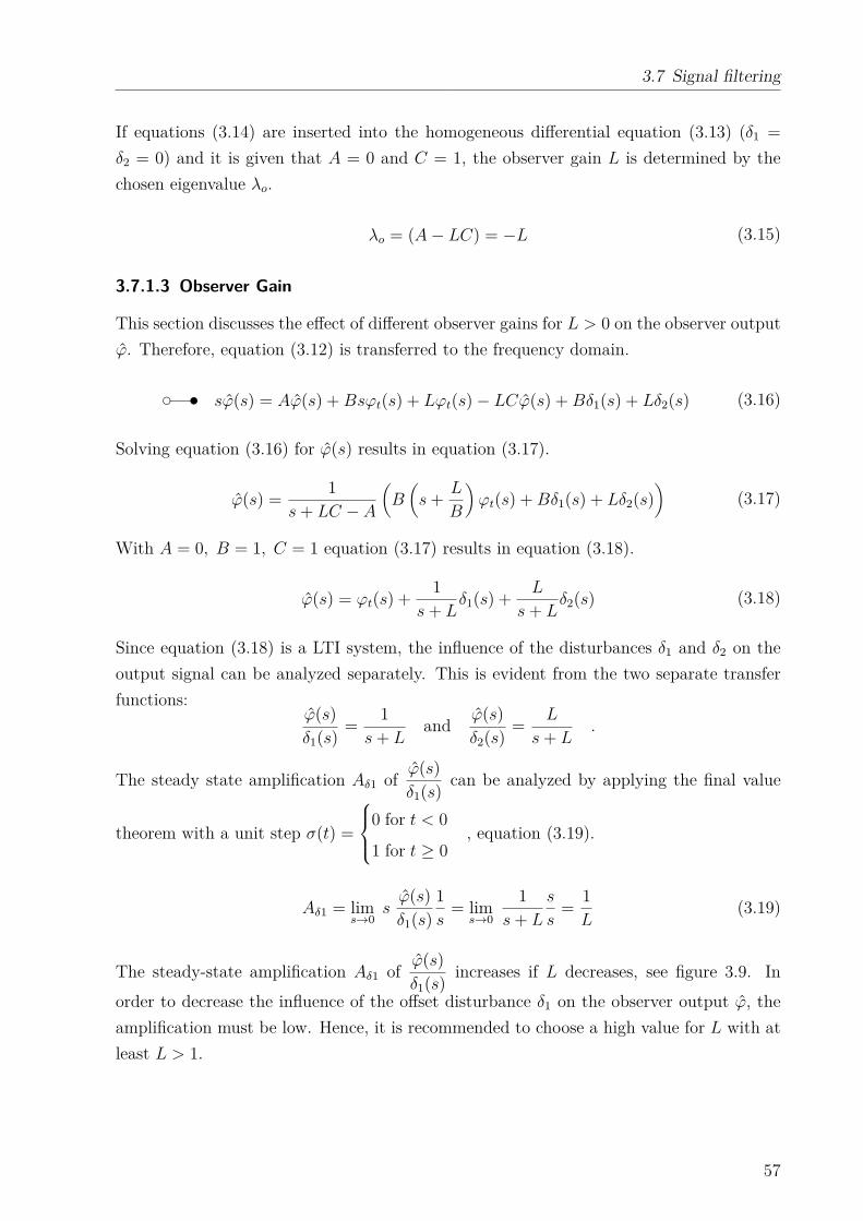
3.7 Signal filtering
If equations (3.14) are inserted into the homogeneous differential equation (3.13) (δ1 =
δ2 = 0) and it is given that A = 0 and C = 1, the observer gain L is determined by the
chosen eigenvalue λo.
λo = (A − LC) = −L (3.15)
3.7.1.3 Observer Gain
This section discusses the effect of different observer gains for L > 0 on the observer output
ϕ. Therefore, equation (3.12) is transferred to the frequency domain.
❞ t sϕ(s) = Aϕ(s) + Bsϕt(s) + Lϕt(s) − LCϕ(s) + Bδ1(s) + Lδ2(s) (3.16)
Solving equation (3.16) for ϕ(s) results in equation (3.17).
ϕ(s) =1
s + LC − A
(
B(
s +L
B
)
ϕt(s) + Bδ1(s) + Lδ2(s))
(3.17)
With A = 0, B = 1, C = 1 equation (3.17) results in equation (3.18).
ϕ(s) = ϕt(s) +1
s + Lδ1(s) +
L
s + Lδ2(s) (3.18)
Since equation (3.18) is a LTI system, the influence of the disturbances δ1 and δ2 on the
output signal can be analyzed separately. This is evident from the two separate transfer
functions:ϕ(s)
δ1(s)=
1
s + Land
ϕ(s)
δ2(s)=
L
s + L.
The steady state amplification Aδ1 ofϕ(s)
δ1(s)can be analyzed by applying the final value
theorem with a unit step σ(t) =
0 for t < 0
1 for t ≥ 0, equation (3.19).
Aδ1 = lims→0
sϕ(s)
δ1(s)
1
s= lim
s→0
1
s + L
s
s=
1
L(3.19)
The steady-state amplification Aδ1 ofϕ(s)
δ1(s)increases if L decreases, see figure 3.9. In
order to decrease the influence of the offset disturbance δ1 on the observer output ϕ, the
amplification must be low. Hence, it is recommended to choose a high value for L with at
least L > 1.
57
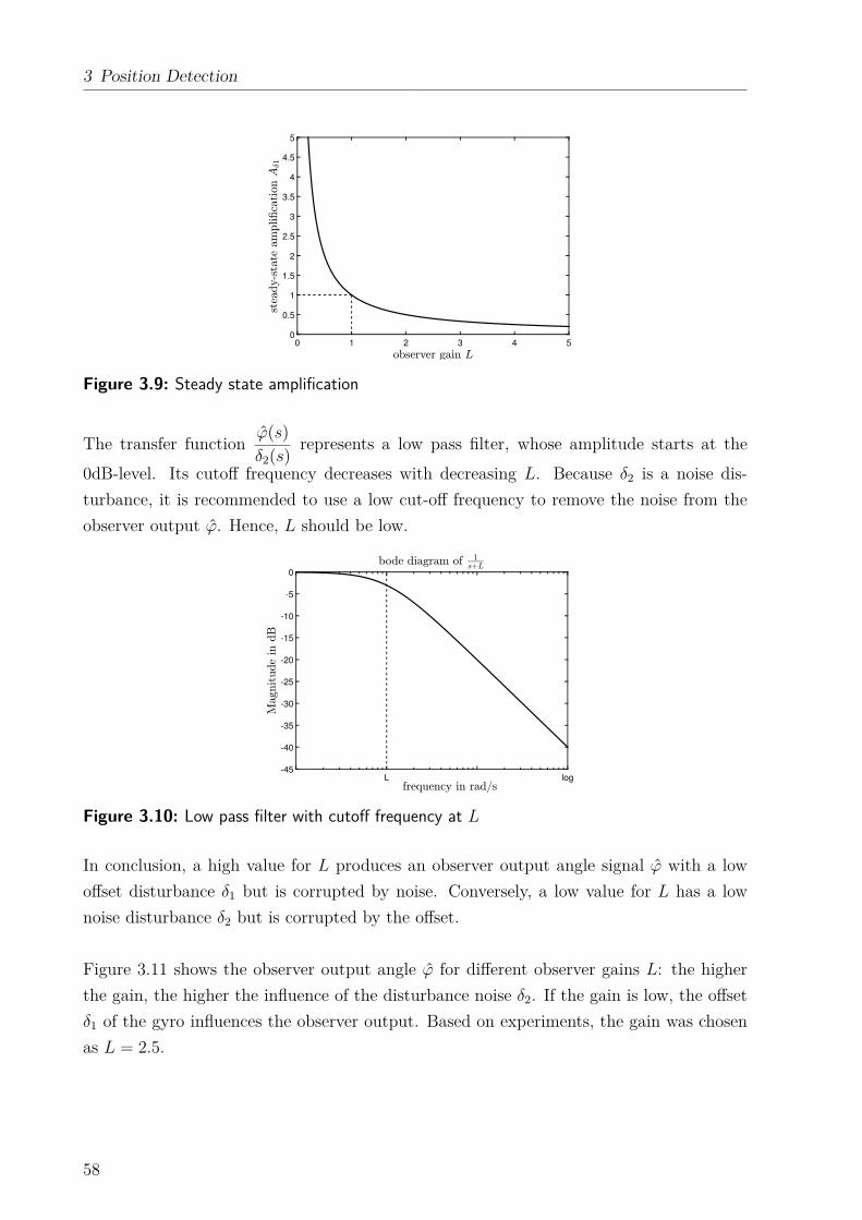
3 Position Detection
0 1 2 3 4 50
0.5
1
1.5
2
2.5
3
3.5
4
4.5
5
Figure 3.9: Steady state amplification
The transfer functionϕ(s)
δ2(s)represents a low pass filter, whose amplitude starts at the
0dB-level. Its cutoff frequency decreases with decreasing L. Because δ2 is a noise dis-
turbance, it is recommended to use a low cut-off frequency to remove the noise from the
observer output ϕ. Hence, L should be low.
L log-45
-40
-35
-30
-25
-20
-15
-10
-5
0
Figure 3.10: Low pass filter with cutoff frequency at L
In conclusion, a high value for L produces an observer output angle signal ϕ with a low
offset disturbance δ1 but is corrupted by noise. Conversely, a low value for L has a low
noise disturbance δ2 but is corrupted by the offset.
Figure 3.11 shows the observer output angle ϕ for different observer gains L: the higher
the gain, the higher the influence of the disturbance noise δ2. If the gain is low, the offset
δ1 of the gyro influences the observer output. Based on experiments, the gain was chosen
as L = 2.5.
58
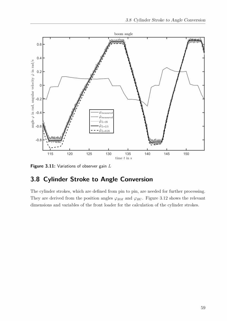
3.8 Cylinder Stroke to Angle Conversion
115 120 125 130 135 140 145 150
-0.8
-0.6
-0.4
-0.2
0
0.2
0.4
0.6
Figure 3.11: Variations of observer gain L
3.8 Cylinder Stroke to Angle Conversion
The cylinder strokes, which are defined from pin to pin, are needed for further processing.
They are derived from the position angles ϕBM and ϕBU . Figure 3.12 shows the relevant
dimensions and variables of the front loader for the calculation of the cylinder strokes.
59
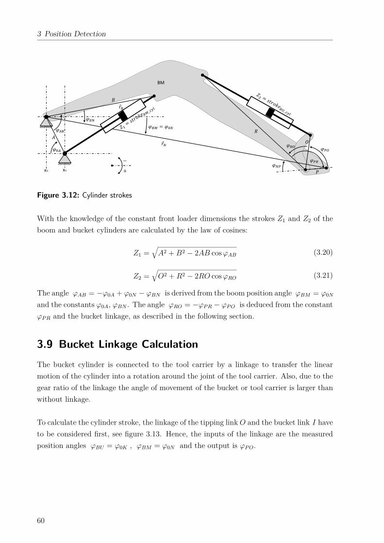
3 Position Detection
xO xU
BM
−+ �
��� ��� = �0� ��0
���
� ��
Figure 3.12: Cylinder strokes
With the knowledge of the constant front loader dimensions the strokes Z1 and Z2 of the
boom and bucket cylinders are calculated by the law of cosines:
Z1 =√
A2 + B2 − 2AB cos ϕAB (3.20)
Z2 =√
O2 + R2 − 2RO cos ϕRO (3.21)
The angle ϕAB = −ϕ0A + ϕ0N − ϕBN is derived from the boom position angle ϕBM = ϕ0N
and the constants ϕ0A, ϕBN . The angle ϕRO = −ϕP R − ϕP O is deduced from the constant
ϕP R and the bucket linkage, as described in the following section.
3.9 Bucket Linkage Calculation
The bucket cylinder is connected to the tool carrier by a linkage to transfer the linear
motion of the cylinder into a rotation around the joint of the tool carrier. Also, due to the
gear ratio of the linkage the angle of movement of the bucket or tool carrier is larger than
without linkage.
To calculate the cylinder stroke, the linkage of the tipping link O and the bucket link I have
to be considered first, see figure 3.13. Hence, the inputs of the linkage are the measured
position angles ϕBU = ϕ0K , ϕBM = ϕ0N and the output is ϕP O.
60
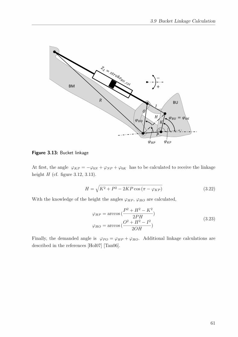
3.9 Bucket Linkage Calculation
BM
BU
��
�� ��
�
−+
��� = �0�
Figure 3.13: Bucket linkage
At first, the angle ϕKP = −ϕ0N + ϕNP + ϕ0K has to be calculated to receive the linkage
height H (cf. figure 3.12, 3.13).
H =√
K2 + P 2 − 2KP cos (π − ϕKP ) (3.22)
With the knowledge of the height the angles ϕHP , ϕHO are calculated,
ϕHP = arccos (P 2 + H2 − K2
2PH)
ϕHO = arccos (O2 + H2 − I2
2OH)
(3.23)
Finally, the demanded angle is ϕP O = ϕHP + ϕHO. Additional linkage calculations are
described in the references [Hol07] [Tan06].
61

4 Weighing Function
The dynamic, continuous, and center of gravity independent weighing system describes
the approach of a mobile scale that measures payload continuously in standard working
conditions of a loader. The result is independent of the center of gravity of the payload
and machine movements. In order to achieve this goal, the approach combines two major
models. On the one hand, cylinder forces are measured continuously and transferred to
torques by using a static model. On the other hand, a multi-body model of the front
loader is created to generate cylinder forces and torques on the joints based on continuously
measured accelerations. The output of both models are merged together. The deviation
between the two models is the basis for the payload calculation. Splitting the weighing
approach into two models provides transferability to different kind of loaders. Thus, only
the static model has to be adapted to a different loader. The multi-body model is reduced
and parameterized with a calibration function which is explained later in section 4.6.2.
The proceeding and structure of this chapter is illustrated in figure 4.1. First, the static
model is described which uses the cylinder forces to calculate torques at the front loader
main joints. The static model is subject to friction, hence, the friction modeling is explained
in detail. Secondly, a detailed multi-body model is discussed which is used to transform
measured accelerations into torques at the loader joints. Thirdly, the static model and
the multi-body model are merged to calculate the payload mL, which is illustrated with
a simplified example. Fourthly, it is explained how the algorithms are simplified and
implemented in order to run them on a real time controller that is applied on a tractor
prototype.
63
4 Weighing Function
The multi-body model is very detailed in order to achieve high accuracy. The parameter
identification of the multi-body model consumes a lot of time and effort. The subsequent
mounting of an additional part to the front loader makes it necessary to identify the pa-
rameters again. Additionally, in serial production each front loader is subject to tolerances,
which requires to identify the parameters for each front loader separately. Because this
is difficult to accomplish, a reduced multi-body model is developed which obtains its
parameters from CAD and a short calibration procedure. This calibration procedure can
also be automated.
multi-body model,
section 4.2.2.1
reduced multi-body
model, section 4.6
weighing algorithm, section 4.3 mL
static model, section 4.1
friction model-
ing, section 4.1.2.2
Figure 4.1: Structure of the weighing function
4.1 Static Model
The static model is used to transfer continuously measured cylinder forces into torques
at the front loader main joints. In order to achieve this, the cylinder forces, which in-
clude friction, are considered as quasi-static condition. Thus, the static calculations are
performed on the front loader structure, which allows to transfer the real front loader kine-
matics into simplified front loader kinematics. The simplified front loader kinematics is an
open, planar kinematic chain which consists of three segments: the chassis (T), the boom
(BM) and the bucket or tool carrier (BU). Each segment is connected to the next one by a
rotational joint. The torques at the joints keep the kinematic front loader chain in position.
Figure 4.2a shows a standard non-self-leveling front loader kinematics. The cylinders,
here shown as arrows e.g. strokeBM_cyl, can be treated as prismatic joints. Below, in
figure 4.2b, the simplified loader kinematic model is shown.
64
4.1 Static Model
J7
K
P
K2
O
I
S
A
R G
xO xU
yO
yU
��� = �0
BM
BU
���_��� �
��
�� �
���_���J1
J2
J3
J4
J5
J6
J8
K2BM
BU
�ϕ
J1
J2
a)
b)
��� = �0��� = �0�
��� = �0�Figure 4.2: Front loader kinematics
The static model of the loader deals with all dimensions and cylinder forces. With the
knowledge of the constraints and positions, the cylinder forces ~FBM_cyl and ~FBU_cyl can
be transferred into torques, ~TQ1 and ~TQ2, at the joints J1 between tractor and boom or
J2 between boom and bucket. As a result, the inputs are forces and outputs are torques
on a simplified loader kinematic. Any kind of front loader can be used for this approach
whether it is self-leveling or non-self-leveling, as long as it is transferred into the simplified
loader kinematics.
4.1.1 Cylinder Forces
As mentioned before, the static model transfers continuously measured cylinder forces into
torques at the main joints of the loader. The applied method in this thesis calculates the
cylinder forces Fcyl by measuring hydraulic pressures in the cylinders. It is very important
to measure these pressures as closely as possible to the cylinder. This reduces influences
of pressure drop between sensor and cylinder, which is generated by the oil flow due to
the oil viscosity. it is even better to measure inside the cylinder or on a separate cylinder
port. This procedure helps to completely avoid the influence of pressure drop. Since the oil
viscosity is dependent on the hydraulic oil temperature, the disturbances of both variables
have a reduced influence on the measured cylinder force.
65
4 Weighing Function
The force Fcyl of the hydraulic differential cylinders
Fcyl = pAAA − pBAB − Ffriction − macyl (4.1)
is calculated by the pressures p and the respective area A at the piston side “A” and the
rod side “B”, see figure 4.3. The parameters of the cylinders are specified in table A.5 in
the appendix.
Due to the sealing, the cylinder force is reduced by the friction Ffriction, which is ex-
plained in-depth in chapter 2.9.1. During movement, the inertial force macyl has to be
considered, too. In this thesis, the inertial force is considered by the multi-body model.
Hence, the cylinder will be treated without mass.
���
�� �� ��
�
� ��
Figure 4.3: Cylinder force
If the cylinder is at the minimum or maximum end-stroke position, as shown in figure
4.4, it is not possible to measure Fcyl by the hydraulic pressures. In this case, the forces
are partly supported by the cylinder walls. If the cylinder is close to the end-stroke and
equipped with an end-stroke damping, it is also not possible to measure Fcyl.� =?Figure 4.4: Cylinder end-stroke
To measure the cylinder force continuously, the end-stroke positions have to be avoided.
See also [Fin06], [WG08], and [Wat07].
A preferable alternative method is to measure Fcyl with strain gauges applied on a ho-
mogeneous position of the cylinder rod. This approach avoids the influence of the cylinder
seal friction on the actuator force measurement. It is meaningful to reduce parts between
the point of measuring and the joint, where the torque is calculated. For instance, the
torque at the bucket joint J2 is calculated by measuring the bucket cylinder forces. To
66
4.1 Static Model
calculate this torque, the bucket linkage with all its joints has to be considered. It can be
said that the less pivots have to be considered in the calculation the less friction disturbs
the result. Accordingly, the strain gauges could be applied directly at the upper bucket
linkage (figure 4.2 (a) part I). A further advantage of this method is that the force mea-
surement can be performed in every cylinder position even in the end-stroke position. The
disadvantage of this method is the time-consuming bonding and calibration of the strain
gauges. Moreover, the calibration of the strain gauges requires a test bench, which applies
known test loads to the cylinder.
4.1.2 Friction
The payload measurement is performed dynamically, hence, friction in the cylinders and
joints or bearings have to be taken into account. The friction at the joints and hydraulic
cylinders is different for each front loader. This is caused by many aspects, for exam-
ple, by manufacturing tolerances, by wear due to the number of operation hours, or by
temperature.
4.1.2.1 Approach of Friction Modeling
Friction compensation is a very basic problem of the payload weighing system. There are
different methods to consider friction. A common way is to design friction with a dynamic
friction model as described in section 2.9.4.2. If the system is in a steady condition, for
instance, when the actuator does not accelerate, the dynamic friction model is equal to
the steady state friction model as described in section 2.9.4.1. The dynamic friction model
needs a high sample rate to model the transient response of pre-displacement which makes
it difficult to implement the dynamic friction model for a common real time controller.
A friction observer as described in [TASLH08] is inappropriate for the weighing system
because, generally, a dynamic model with known inertial mass is needed. A friction ob-
server calculates the friction force with the knowledge of the input actuator force and the
acceleration of the inertial mass. If the mass changes, the system experiences different
accelerations which are concluded as a different friction force instead of a different mass.
In this case, the mass (payload) changes permanently and has to be calculated. Hence
the friction force must be modeled. The accuracy of the friction is strongly related to the
accuracy of friction model parameters, which are generally obtained from empirical data.
Hence, it is meaningful to reduce the parameters to those which are easy to identify in tests.
In order to consider friction, this thesis develops a steady state friction model which is
based on the “Pressure Based Model” of section 2.9.4.3. The friction model is parameter-
67
4 Weighing Function
ized with data which is obtained from tests with the loader. Basically, the Coulomb friction
in the steady state friction model (cf. section 2.9.4.1) is replaced by the “Pressure Based
Model”. The stiction is not considered because measurements show that stiction is in-
significantly low except directly after longer standstill of the loader. This can be explained
by the decreasing lubrication film between the sliding partners when standing still. Also,
measurements show that the cylinder forces change during standstill (cf. section A.6). For
example, after moving the boom upward the seal friction acts against the movement, which
is downward. During standstill, the cylinder drifts downward which causes the seal friction
to act upward. Because the drift is too small to detect, it is not possible to define the
direction of the friction. For this reason, it is not yet possible to consider friction during
standstill of the front loader. Hence, stiction is not considered. Also, the viscous friction,
which is dependent on the actuator velocity, is neglected. However, the influence of the
actuator velocity is considered indirectly as explained in the following section.
4.1.2.2 Procedure of Friction Modeling
The total friction is a sum of bearing frictions and seal frictions. The friction generated
by the bearings is low compared to the total friction (cf. section A.10). Thus, the cylinder
seals are primarily responsible for the friction and the total friction is treated as if it is
only related to the cylinders.
It is assumed that the amount of friction is symmetrical. That means the absolute friction
of a boom down movement is the same as of a boom up movement as long as the load and
the corresponding cylinder pressures remain constant. This assumption is based on the
friction of the piston seals, which are built symmetrically in both directions, and due to
the bearings, which ideally have the same amount of friction no matter in which direction
they turn (cf. section 2.9.3). The rod seal is built asymmetrically. Therefore, the friction
of the rod seal also varies from in- to out-movement of the actuator. This is simplified by
treating friction of the rod seal symmetrically.
In order to identify the overall friction the tractor needs to stand still and only the front
loader moves up and down with a constant cylinder velocity. Due to the quasi-static
condition, all acceleration terms will be zero and the force balance will be as follows (cf.
figure 4.5):
Fcyl_raw = Fcyl − Ffriction (4.2)
The raw cylinder force Fcyl_raw is calculated by the cylinder pressures pA, pB and its area
dimensions AA, AB. (index “A” stands for the piston side and index “B” stands for the
68
4.1 Static Model
rod side)
Fcyl_raw = FA − FB = pAAA − pBAB (4.3)
� _�
���
� _�
�� �� ��
��
� � = � �
Figure 4.5: Cylinder force
The mass of the front loader and the position of the tractor are constant during the
measurement. Hence, the force Fload, and along with it Fcyl, are only functions of the
loader position or cylinder stroke. To evaluate the friction, several up and down cycles
with different cylinder velocities velcyl are performed. During the movement, pressures are
recorded and the force Fcyl_raw is calculated, as displayed in figure 4.6.
69
4 Weighing Function
1.05 1.1 1.15 1.2 1.25 1.3 1.35 1.4 1.45
104
1.7
1.8
1.9
2
2.1
2.2
2.3
2.4
2.5
2.6
2.7
2.8
Figure 4.6: Cylinder force over boom cylinder stroke
The friction wants to hold the front loader in its position and works against the movement.
If the cylinder speed is positive velcyl > 0, the boom moves upward and the measured
cylinder force Fcyl_raw is higher than the force Fload due to the friction. If the boom moves
downward the cylinder force is lower than Fload.
The force Fload can be obtained by the multi-body model of the front loader, but the
model is not accurate enough. Also, due to manufacturing tolerances, the model parame-
ters slightly change at different front loaders. Thus, the boom of the empty front loader is
moved up and down very slowly (velcyl ≈ 0.015m/s) and the force Fload is approximated
by the mean value of the forces Fcyl_raw for up and down movement.
Fload ≈ Fcyl_mean =Fcyl_raw up slow + Fcyl_raw down slow
2(4.4)
The approximated force Fload is more accurate if the difference between the raw forces
Fcyl_raw up/down slow is kept as small as possible. This can be achieved by moving the front
70
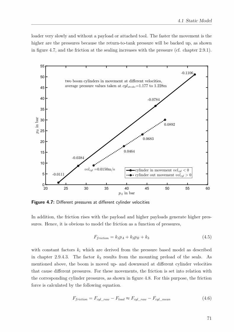
4.1 Static Model
loader very slowly and without a payload or attached tool. The faster the movement is the
higher are the pressures because the return-to-tank pressure will be backed up, as shown
in figure 4.7, and the friction at the sealing increases with the pressure (cf. chapter 2.9.1).
20 25 30 35 40 45 50 55 60
0
5
10
15
20
25
30
35
40
45
50
55
Figure 4.7: Different pressures at different cylinder velocities
In addition, the friction rises with the payload and higher payloads generate higher pres-
sures. Hence, it is obvious to model the friction as a function of pressures,
Ffriction = k1pA + k2pB + k3 (4.5)
with constant factors ki which are derived from the pressure based model as described
in chapter 2.9.4.3. The factor k3 results from the mounting preload of the seals. As
mentioned above, the boom is moved up- and downward at different cylinder velocities
that cause different pressures. For these movements, the friction is set into relation with
the corresponding cylinder pressures, as shown in figure 4.8. For this purpose, the friction
force is calculated by the following equation.
Ffriction = Fcyl_raw − Fload ≈ Fcyl_raw − Fcyl_mean (4.6)
71
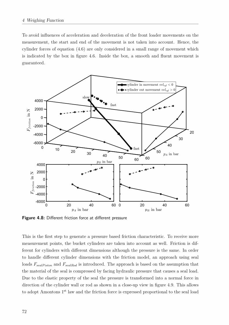
4 Weighing Function
To avoid influences of acceleration and deceleration of the front loader movements on the
measurement, the start and end of the movement is not taken into account. Hence, the
cylinder forces of equation (4.6) are only considered in a small range of movement which
is indicated by the box in figure 4.6. Inside the box, a smooth and fluent movement is
guaranteed.
20
30
40
50
6060
5040
3020
100
-2000
-4000
-6000
0
4000
2000
0 20 40 60
-6000
-4000
-2000
0
2000
4000
0 20 40 60
Figure 4.8: Different friction force at different pressure
This is the first step to generate a pressure based friction characteristic. To receive more
measurement points, the bucket cylinders are taken into account as well. Friction is dif-
ferent for cylinders with different dimensions although the pressure is the same. In order
to handle different cylinder dimensions with the friction model, an approach using seal
loads FsealP iston and FsealRod is introduced. The approach is based on the assumption that
the material of the seal is compressed by facing hydraulic pressure that causes a seal load.
Due to the elastic property of the seal the pressure is transformed into a normal force in
direction of the cylinder wall or rod as shown in a close-up view in figure 4.9. This allows
to adopt Amontons 1st law and the friction force is expressed proportional to the seal load
72
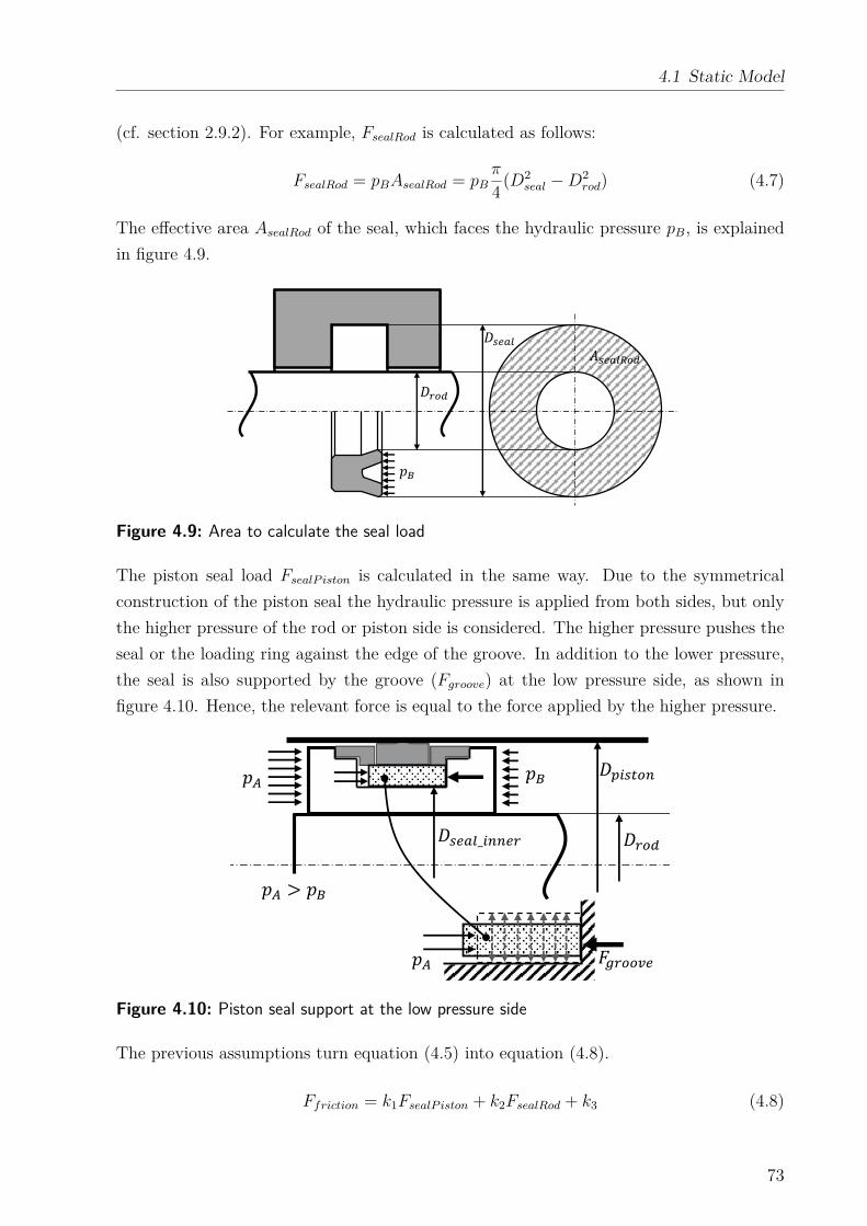
4.1 Static Model
(cf. section 2.9.2). For example, FsealRod is calculated as follows:
FsealRod = pBAsealRod = pBπ
4(D2
seal − D2rod) (4.7)
The effective area AsealRod of the seal, which faces the hydraulic pressure pB, is explained
in figure 4.9.
�
� �����
Figure 4.9: Area to calculate the seal load
The piston seal load FsealP iston is calculated in the same way. Due to the symmetrical
construction of the piston seal the hydraulic pressure is applied from both sides, but only
the higher pressure of the rod or piston side is considered. The higher pressure pushes the
seal or the loading ring against the edge of the groove. In addition to the lower pressure,
the seal is also supported by the groove (Fgroove) at the low pressure side, as shown in
figure 4.10. Hence, the relevant force is equal to the force applied by the higher pressure.
� � � ����> �
� _� �
� ���Figure 4.10: Piston seal support at the low pressure side
The previous assumptions turn equation (4.5) into equation (4.8).
Ffriction = k1FsealP iston + k2FsealRod + k3 (4.8)
73
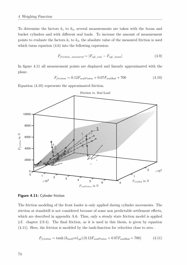
4 Weighing Function
To determine the factors k1 to k3, several measurements are taken with the boom and
bucket cylinders and with different seal loads. To increase the amount of measurement
points to evaluate the factors k1 to k3, the absolute value of the measured friction is used
which turns equation (4.6) into the following expression:
Ffriction_measured = |Fcyl_raw − Fcyl_mean| (4.9)
In figure 4.11 all measurement points are displayed and linearly approximated with the
plane.
Ffriction = 0.12FsealP iston + 0.07FsealRod + 700 (4.10)
Equation (4.10) represents the approximated friction.
1042
1
065
43
2
104
10
4000
0
2000
10000
8000
6000
Figure 4.11: Cylinder friction
The friction modeling of the front loader is only applied during cylinder movements. The
stiction at standstill is not considered because of some non predictable settlement effects,
which are described in appendix A.6. Thus, only a steady state friction model is applied
(cf. chapter 2.9.4). The final friction, as it is used in this thesis, is given by equation
(4.11). Here, the friction is modeled by the tanh-function for velocities close to zero .
Ffriction = tanh (ktanhvelcyl) (0.12FsealP iston + 0.07FsealRod + 700) (4.11)
74
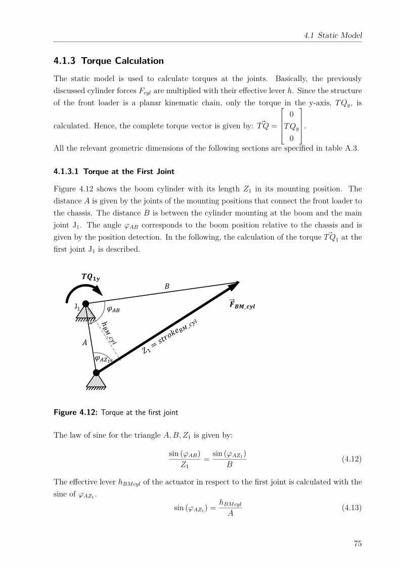
4.1 Static Model
4.1.3 Torque Calculation
The static model is used to calculate torques at the joints. Basically, the previously
discussed cylinder forces Fcyl are multiplied with their effective lever h. Since the structure
of the front loader is a planar kinematic chain, only the torque in the y-axis, TQy, is
calculated. Hence, the complete torque vector is given by: ~TQ =
0
TQy
0
.
All the relevant geometric dimensions of the following sections are specified in table A.3.
4.1.3.1 Torque at the First Joint
Figure 4.12 shows the boom cylinder with its length Z1 in its mounting position. The
distance A is given by the joints of the mounting positions that connect the front loader to
the chassis. The distance B is between the cylinder mounting at the boom and the main
joint J1. The angle ϕAB corresponds to the boom position relative to the chassis and is
given by the position detection. In the following, the calculation of the torque ~TQ1 at the
first joint J1 is described.
J1
����_���
� �� �
� ���_�����
� ��
� � ���_� �
�
� � �� �
� �
�Figure 4.12: Torque at the first joint
The law of sine for the triangle A, B, Z1 is given by:
sin (ϕAB)
Z1
=sin (ϕAZ1
)
B(4.12)
The effective lever hBMcyl of the actuator in respect to the first joint is calculated with the
sine of ϕAZ1.
sin (ϕAZ1) =
hBMcyl
A(4.13)
75
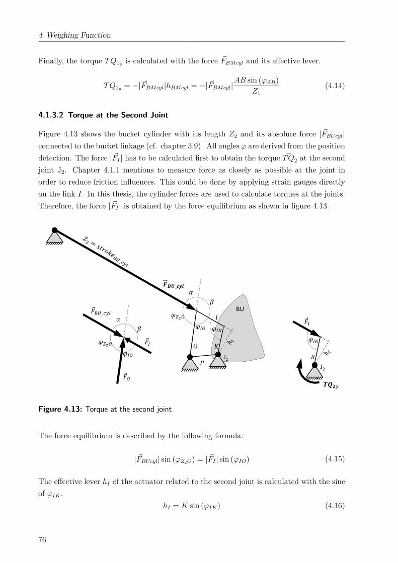
4 Weighing Function
Finally, the torque TQ1yis calculated with the force ~FBMcyl and its effective lever.
TQ1y= −| ~FBMcyl|hBMcyl = −| ~FBMcyl|
AB sin (ϕAB)
Z1
(4.14)
4.1.3.2 Torque at the Second Joint
Figure 4.13 shows the bucket cylinder with its length Z2 and its absolute force | ~FBUcyl|connected to the bucket linkage (cf. chapter 3.9). All angles ϕ are derived from the position
detection. The force | ~FI | has to be calculated first to obtain the torque ~TQ2 at the second
joint J2. Chapter 4.1.1 mentions to measure force as closely as possible at the joint in
order to reduce friction influences. This could be done by applying strain gauges directly
on the link I. In this thesis, the cylinder forces are used to calculate torques at the joints.
Therefore, the force | ~FI | is obtained by the force equilibrium as shown in figure 4.13.
����_���
� �� �
�BU
J2
���_�����
� ��
� � ���_� �
�
� �
J2
�� �
� �
�J2
J2
Figure 4.13: Torque at the second joint
The force equilibrium is described by the following formula:
| ~FBUcyl| sin (ϕZ2O) = | ~FI | sin (ϕIO) (4.15)
The effective lever hI of the actuator related to the second joint is calculated with the sine
of ϕIK .
hI = K sin (ϕIK) (4.16)
76
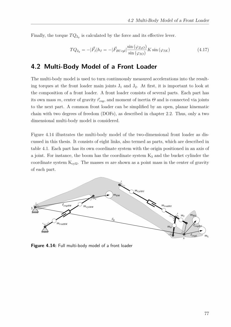
4.2 Multi-Body Model of a Front Loader
Finally, the torque TQ2yis calculated by the force and its effective lever.
TQ2y= −| ~FI |hI = −| ~FBUcyl|
sin (ϕZ2O)
sin (ϕIO)K sin (ϕIK) (4.17)
4.2 Multi-Body Model of a Front Loader
The multi-body model is used to turn continuously measured accelerations into the result-
ing torques at the front loader main joints J1 and J2. At first, it is important to look at
the composition of a front loader. A front loader consists of several parts. Each part has
its own mass m, center of gravity ~rcog, and moment of inertia Θ and is connected via joints
to the next part. A common front loader can be simplified by an open, planar kinematic
chain with two degrees of freedom (DOFs), as described in chapter 2.2. Thus, only a two
dimensional multi-body model is considered.
Figure 4.14 illustrates the multi-body model of the two-dimensional front loader as dis-
cussed in this thesis. It consists of eight links, also termed as parts, which are described in
table 4.1. Each part has its own coordinate system with the origin positioned in an axis of
a joint. For instance, the boom has the coordinate system K3 and the bucket cylinder the
coordinate system Kcyl2. The masses m are shown as a point mass in the center of gravity
of each part.
� � � ��
� � � � ��
��
�� ��
����
�� ����
J1
J2Figure 4.14: Full multi-body model of a front loader
77
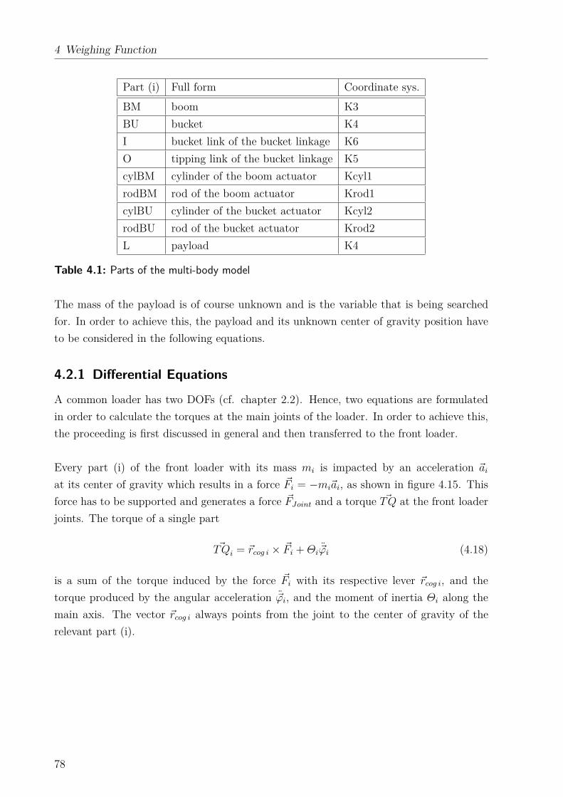
4 Weighing Function
Part (i) Full form Coordinate sys.
BM boom K3
BU bucket K4
I bucket link of the bucket linkage K6
O tipping link of the bucket linkage K5
cylBM cylinder of the boom actuator Kcyl1
rodBM rod of the boom actuator Krod1
cylBU cylinder of the bucket actuator Kcyl2
rodBU rod of the bucket actuator Krod2
L payload K4
Table 4.1: Parts of the multi-body model
The mass of the payload is of course unknown and is the variable that is being searched
for. In order to achieve this, the payload and its unknown center of gravity position have
to be considered in the following equations.
4.2.1 Differential Equations
A common loader has two DOFs (cf. chapter 2.2). Hence, two equations are formulated
in order to calculate the torques at the main joints of the loader. In order to achieve this,
the proceeding is first discussed in general and then transferred to the front loader.
Every part (i) of the front loader with its mass mi is impacted by an acceleration ~ai
at its center of gravity which results in a force ~Fi = −mi~ai, as shown in figure 4.15. This
force has to be supported and generates a force ~FJoint and a torque ~TQ at the front loader
joints. The torque of a single part
~TQi = ~rcog i × ~Fi + Θi ~ϕi (4.18)
is a sum of the torque induced by the force ~Fi with its respective lever ~rcog i, and the
torque produced by the angular acceleration ~ϕi, and the moment of inertia Θi along the
main axis. The vector ~rcog i always points from the joint to the center of gravity of the
relevant part (i).
78
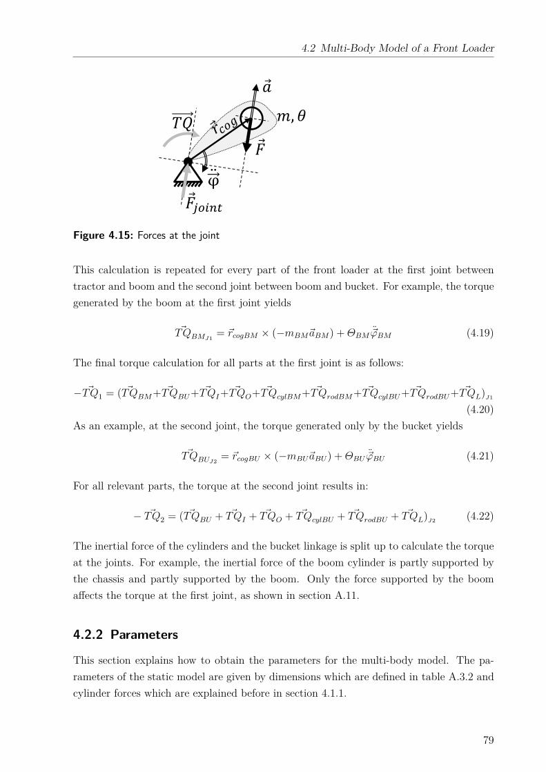
4.2 Multi-Body Model of a Front Loader � , � � � �� φ
Figure 4.15: Forces at the joint
This calculation is repeated for every part of the front loader at the first joint between
tractor and boom and the second joint between boom and bucket. For example, the torque
generated by the boom at the first joint yields
~TQBMJ1= ~rcogBM × (−mBM~aBM) + ΘBM ~ϕBM (4.19)
The final torque calculation for all parts at the first joint is as follows:
− ~TQ1 = ( ~TQBM + ~TQBU + ~TQI+ ~TQO+ ~TQcylBM + ~TQrodBM + ~TQcylBU + ~TQrodBU + ~TQL)J1
(4.20)
As an example, at the second joint, the torque generated only by the bucket yields
~TQBUJ2= ~rcogBU × (−mBU~aBU) + ΘBU ~ϕBU (4.21)
For all relevant parts, the torque at the second joint results in:
− ~TQ2 = ( ~TQBU + ~TQI + ~TQO + ~TQcylBU + ~TQrodBU + ~TQL)J2
(4.22)
The inertial force of the cylinders and the bucket linkage is split up to calculate the torque
at the joints. For example, the inertial force of the boom cylinder is partly supported by
the chassis and partly supported by the boom. Only the force supported by the boom
affects the torque at the first joint, as shown in section A.11.
4.2.2 Parameters
This section explains how to obtain the parameters for the multi-body model. The pa-
rameters of the static model are given by dimensions which are defined in table A.3.2 and
cylinder forces which are explained before in section 4.1.1.
79
4 Weighing Function
As mentioned before, the multi-body model is used to transfer measured accelerations
into resulting torques at the front loader main joints. Hence, the translational accelera-
tion, angular acceleration, and angular velocity are measured continuously with an IMU.
Furthermore, the position of the front loader is needed, which is continuously provided by
the position detection as described in chapter 3. The relative movements and accelerations
between the loader parts are necessary to calculate the accelerations for each center of
gravity, as explained in the following section. These relative movements and accelerations
can be derived from the position detection. Alternatively, they can be continuously mea-
sured by subtracting the angular velocities and angular accelerations of different IMUs as
applied in this thesis. All other parameters such as masses, inertia, and dimensions are
constants and defined once before installing the weighing system.
4.2.2.1 Accelerations
The acceleration ~a can be measured with a sensor at any position. The accelerations ~ai for
each center of gravity are calculated with the knowledge of the angular velocity ϕ, angular
acceleration ϕ, center of gravity positions, and front loader movements. For example,
section 2.6.4 demonstrates the calculation of the acceleration for any point at the tractor
with IMU S2. In this thesis, the boom IMU S3 is used to calculate the accelerations ~ai
for each center of gravity of the front loader as illustrated in figure 4.16. As an example,
equation (2.20) is converted to calculate the acceleration ~aP with IMU S3 for any point at
the boom:
~aP = ~r1P = ~r1S3 + ~ϕS3 ×(
~ϕS3 × [~r3P − ~r3S3])
+ ~ϕS3 × [~r3P − ~r3S3]
~aP = ~r1P = ~r1S3 + ~ϕS3 ×(
~ϕ2 × [~rS3P ])
+ ~ϕS3 × [~rS3P ] (4.23)
80
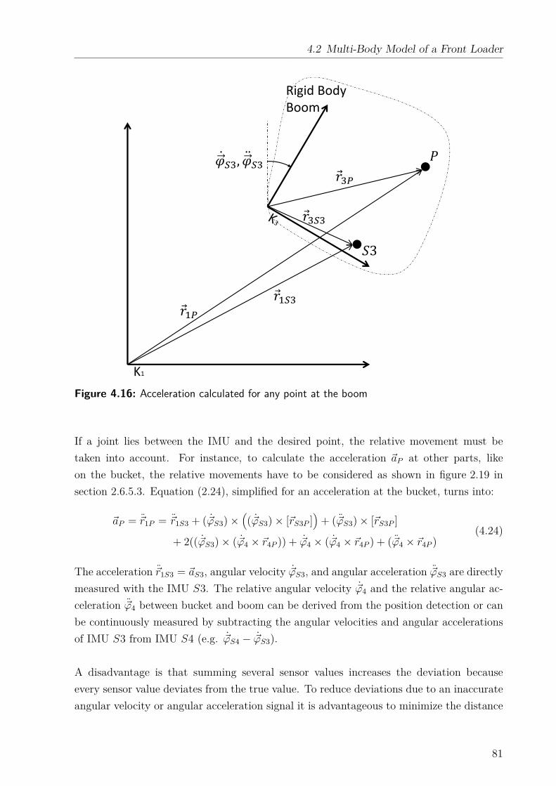
4.2 Multi-Body Model of a Front Loader
K1
�
� � , �
� �
Rigid Body
Boom
Figure 4.16: Acceleration calculated for any point at the boom
If a joint lies between the IMU and the desired point, the relative movement must be
taken into account. For instance, to calculate the acceleration ~aP at other parts, like
on the bucket, the relative movements have to be considered as shown in figure 2.19 in
section 2.6.5.3. Equation (2.24), simplified for an acceleration at the bucket, turns into:
~aP = ~r1P = ~r1S3 + ( ~ϕS3) ×(
( ~ϕS3) × [~rS3P ])
+ ( ~ϕS3) × [~rS3P ]
+ 2(( ~ϕS3) × ( ~ϕ4 × ~r4P )) + ~ϕ4 × ( ~ϕ4 × ~r4P ) + ( ~ϕ4 × ~r4P )(4.24)
The acceleration ~r1S3 = ~aS3, angular velocity ~ϕS3, and angular acceleration ~ϕS3 are directly
measured with the IMU S3. The relative angular velocity ~ϕ4 and the relative angular ac-
celeration ~ϕ4 between bucket and boom can be derived from the position detection or can
be continuously measured by subtracting the angular velocities and angular accelerations
of IMU S3 from IMU S4 (e.g. ~ϕS4 − ~ϕS3).
A disadvantage is that summing several sensor values increases the deviation because
every sensor value deviates from the true value. To reduce deviations due to an inaccurate
angular velocity or angular acceleration signal it is advantageous to minimize the distance
81
4 Weighing Function
[~rS3P ] between IMU and the point, where the acceleration is calculated for. For the purpose
of this thesis, it is better to place the IMU directly at the center of gravity or at least close
to it at the same part. In order to simplify the calculation, the following rule is applied. If
the IMU is mounted at a different part, as in equation (4.24), and the relative movement
is slow between both parts, the acceleration terms, which consider relative movement, can
be neglected for small parts.
The acceleration ~aL of the payload cannot be defined accurately, because the exact cen-
ter of gravity position ~rcogL_exact of the payload is unknown. Nevertheless, the center of
gravity position of the payload will be close to the bucket or attachment carrier. There-
fore, the acceleration ~aL is calculated with an approximated center of gravity position
~rcogL_exact ≈ ~rcogL as shown in equation (4.25). This procedure is acceptable, because
deviations only arise if the payload experiences angular velocities or angular accelerations
(see also equation (4.36)).
~aL[K3] = ~aS3 + ( ~ϕS3) ×(
( ~ϕS3) × [K4
↓ RK3
~rcogL + ~rN − ~rS3]
)
+ ( ~ϕS3) × [K4
↓ RK3
~rcogL + ~rN − ~rS3]
+ 2(( ~ϕS3) × ( ~ϕ4×K4
↓ RK3
~rcogL)) + ~ϕ4 × ( ~ϕ4×K4
↓ RK3
~rcogL) + ( ~ϕ4×K4
↓ RK3
~rcogL)
(4.25)
It is assumed that the payload is rigidly connected to the bucket or tool carrier. The
acceleration ~aL of a swinging payload, for example, a load hanging on a chain, cannot be
approximated by this approach. In this case, the payload has to be in a steady condition,
which means that the payload must not oscillate. An approach to deal with oscillating
payloads is to use the average of the calculated payload over a few cycles.
As mentioned before, the front loader is simplified to a planar, open kinematic chain
and only movements in the x-z-plane are considered. Therefore, it is sufficient to define
only accelerations in the x- and z-direction for each center of gravity.
4.2.2.2 Mass, Center of Gravity, and Inertia of a Part
The mass m, the center of gravity ~rcog, and the inertia Θ of a part are constant, as long
as the part is not modified. A part is defined as a rigid body including all stiff mounted
add-ons, such as brackets. The boom part, for instance, includes all hoses, fittings and
pins. To obtain an accurate multi-body model, a standard series front loader is taken
apart as shown in figure A.4. For each part the parameters like the mass, the inertia and
the center of gravity are measured as described in section 2.7 Mass and Center of Gravity
82
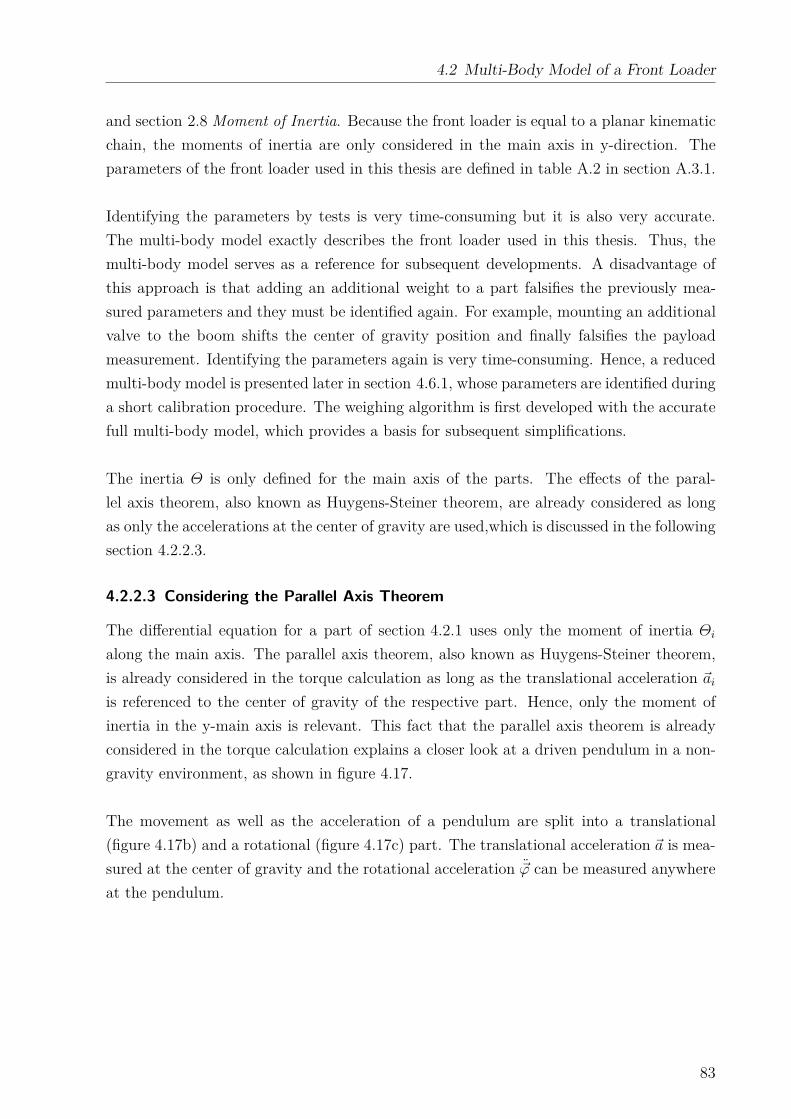
4.2 Multi-Body Model of a Front Loader
and section 2.8 Moment of Inertia. Because the front loader is equal to a planar kinematic
chain, the moments of inertia are only considered in the main axis in y-direction. The
parameters of the front loader used in this thesis are defined in table A.2 in section A.3.1.
Identifying the parameters by tests is very time-consuming but it is also very accurate.
The multi-body model exactly describes the front loader used in this thesis. Thus, the
multi-body model serves as a reference for subsequent developments. A disadvantage of
this approach is that adding an additional weight to a part falsifies the previously mea-
sured parameters and they must be identified again. For example, mounting an additional
valve to the boom shifts the center of gravity position and finally falsifies the payload
measurement. Identifying the parameters again is very time-consuming. Hence, a reduced
multi-body model is presented later in section 4.6.1, whose parameters are identified during
a short calibration procedure. The weighing algorithm is first developed with the accurate
full multi-body model, which provides a basis for subsequent simplifications.
The inertia Θ is only defined for the main axis of the parts. The effects of the paral-
lel axis theorem, also known as Huygens-Steiner theorem, are already considered as long
as only the accelerations at the center of gravity are used,which is discussed in the following
section 4.2.2.3.
4.2.2.3 Considering the Parallel Axis Theorem
The differential equation for a part of section 4.2.1 uses only the moment of inertia Θi
along the main axis. The parallel axis theorem, also known as Huygens-Steiner theorem,
is already considered in the torque calculation as long as the translational acceleration ~ai
is referenced to the center of gravity of the respective part. Hence, only the moment of
inertia in the y-main axis is relevant. This fact that the parallel axis theorem is already
considered in the torque calculation explains a closer look at a driven pendulum in a non-
gravity environment, as shown in figure 4.17.
The movement as well as the acceleration of a pendulum are split into a translational
(figure 4.17b) and a rotational (figure 4.17c) part. The translational acceleration ~a is mea-
sured at the center of gravity and the rotational acceleration ~ϕ can be measured anywhere
at the pendulum.
83
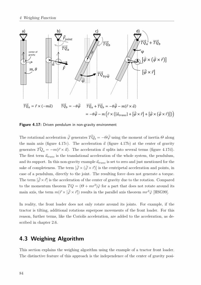
4 Weighing Function
x
z
x
z
� φ � �
� �� +
φ
φ, �
a) b) c) d)
center of
gravity
= � × − � = −� � + = −� � − � × �= −� � − � × � � + � × � + � × � × �
� × � � × � × �
Figure 4.17: Driven pendulum in non-gravity environment
The rotational acceleration ~ϕ generates ~TQb = −Θ~ϕ using the moment of inertia Θ along
the main axis (figure 4.17c). The acceleration ~a (figure 4.17b) at the center of gravity
generates ~TQa = −m(~r × ~a). The acceleration ~a splits into several terms (figure 4.17d).
The first term ~atrans is the translational acceleration of the whole system, the pendulum,
and its support. In this non-gravity example ~atrans is set to zero and just mentioned for the
sake of completeness. The term [ ~ϕ × ( ~ϕ × ~r)] is the centripetal acceleration and points, in
case of a pendulum, directly to the joint. The resulting force does not generate a torque.
The term [ ~ϕ ×~r] is the acceleration of the center of gravity due to the rotation. Compared
to the momentum theorem TQ = (Θ + mr2)ϕ for a part that does not rotate around its
main axis, the term m(~r × [ ~ϕ × ~r]) results in the parallel axis theorem mr2ϕ [HSG99].
In reality, the front loader does not only rotate around its joints. For example, if the
tractor is tilting, additional rotations superpose movements of the front loader. For this
reason, further terms, like the Coriolis acceleration, are added to the acceleration, as de-
scribed in chapter 2.6.
4.3 Weighing Algorithm
This section explains the weighing algorithm using the example of a tractor front loader.
The distinctive feature of this approach is the independence of the center of gravity posi-
84
4.3 Weighing Algorithm
tion of the payload, which is achieved by considering the torque equilibrium at two joints
of an open, planar kinematic chain. Thus, it is possible, to apply the weighing algorithm
also on other systems similar to an open, planar kinematic chain with at least two joints
such as an excavator arm or a loader crane. In addition, the weighing system compensates
disturbances that arise from tractor or front loader movements by considering continuously
measured accelerations.
In order to achieve this, two equilibrium equations are formed using the torque output
of the multi-body model and torque output of the static model. These equations corre-
spond to the first joint J1 between tractor and boom and to the second joint J2 between
boom and bucket. As an example, the multi-body model is simplified and combined with
the simplified kinematic chain of the static model, as shown in figure 4.18. For reasons of
clarity, only the boom and the bucket are considered here. Terms of smaller parts are not
mentioned.
�
mBM
mBU
mL
� � ��
� �
���
��� �
� � ��
� � �� � �
� � ��ϕ
Figure 4.18: Simplified model for the torque equilibrium
The torque output of the static model is set into relation with the torque output of the
multi-body model which generates torques through inertial forces and their respective
levers. The levers are defined by vectors ~rcog, that point from the respective joint to the
center of gravity of the relevant part as described in chapter 4.2.1.
All vectors are referenced to their corresponding part and not to a global inertial co-
ordinate system. For example, ~rcogBM is referenced to the boom coordinate system, which
implies that ~rcogBM is constant. To add or subtract a vector, it has to be transformed to
the same coordinate system K, as shown in chapter 2.4.
For instance: ~rcoordinatesystem3 =K4
↓ RK3
·~rcoordinatensystem4
85
4 Weighing Function
4.3.1 Torque Equilibrium at the First Joint
The torque equilibrium at the first joint is created as follows:
0 = ~TQ1 + [~rcogBM × (−mBM · ~aBM)]
+ [(K4
↓ RK3
·~rcogBU + ~rN) × (−mBU ·K4
↓ RK3
·~aBU)]
+ [(K4
↓ RK3
·~rcogL + ~rN) × (−mL·K4
↓ RK3
·~aL)]
− ΘBM ~ϕS3 − (ΘBU + ΘL) ~ϕS4
(4.26)
The cross product is bilinear and the distributive law can be applied. Hence, it can be
rearranged:
0 = ~TQ1 + [~rcogBM × (−mBM · ~aBM)]
+ [K4
↓ RK3
·~rcogBU × (−mBU ·K4
↓ RK3
·~aBU)] + [~rN × (−mBU ·K4
↓ RK3
·~aBU)]
+ [K4
↓ RK3
·~rcogL × (−mL·K4
↓ RK3
·~aL)] + [~rN × (−mL·K4
↓ RK3
·~aL)]
− ΘBM ~ϕS3 − (ΘBU + ΘL) ~ϕS4
(4.27)
The transformation of coordinates is a rotation around the y-axis. Thus, the cross product
of the transformed vectors is equal to the non-transformed vectors and equation (4.27) can
be simplified to the following term:
0 = ~TQ1 + [~rcogBM × (−mBM · ~aBM)]
+ [~rcogBU × (−mBU · ~aBU)] + [~rN × (−mBU ·K4
↓ RK3
·~aBU)]
+ [~rcogL × (−mL · ~aL)] + [~rN × (−mL·K4
↓ RK3
·~aL)]
− ΘBM ~ϕS3 − (ΘBU + ΘL) ~ϕS4
(4.28)
4.3.2 Torque Equilibrium at the Second Joint
The torque equilibrium at the second joint is given by the following equation:
0 = ~TQ2 + [~rcogBU × (−mBU · ~aBU)] + [~rcogL × (−mL · ~aL)]
− (ΘBU + ΘL) ~ϕS4
(4.29)
86
4.3 Weighing Algorithm
The rearranged equation (4.29) turns into the following term, where all underlined terms
are equal to the underlined terms of equation (4.28):
[~rcogBU × (−mBU · ~aBU)] + [~rcogL × (−mL · ~aL)] − (ΘBU + ΘL) ~ϕS4 = − ~TQ2 (4.30)
4.3.3 Payload Calculation
To obtain the payload mL, the following procedure is applied. Equation (4.30) is inserted
into equation (4.28) which yields the following result:
0 = ~TQ1 + [~rcogBM × (−mBM · ~aBM)]
+ [~rN × (−mBU ·K4
↓ RK3
·~aBU)]
+ [~rN × (−mL·K4
↓ RK3
·~aL)]
− ΘBM ~ϕS3 − ~TQ2
(4.31)
The equation is rearranged and results into:
mL ·[
~rN × (K4
↓ RK3
·~aL)
]
=
[
~TQ1 − ~TQ2 − mBM · [~rcogBM × ~aBM ] − mBU · [~rN × (K4
↓ RK3
·~aBU)] − ΘBM ~ϕS3)
] (4.32)
Since the front loader is similar to an open, planar kinematic chain, every joint has
only one degree of freedom, namely the rotation along the y-axis. Thus, only torques
in the y-direction are considered and all terms turn into vectors of the following form
~TQ =
0
TQy
0
.
By only taking the y-component of the torque vector TQy, the equation (4.32) can be
solved to calculate the payload mL.
mL =TQnum
TQdenum
(4.33)
with
TQnum =[
~TQ1 − ~TQ2 − mBM · [~rcogBM × ~aBM ] − mBU · [~rN × (K4
↓ RK3
·~aBU)] − ΘBM ~ϕS3
]
y
(4.34)
87
4 Weighing Function
and with
TQdenum =
[
~rN × (K4
↓ RK3
·~aL)
]
y
(4.35)
At first glance, the payload is only dependent on dimensions related to the boom, like
~rcogBM and ~rN , which is the distance between the two main joints. A closer examination
reveals that, in order to calculate the acceleration at the bucket, the distance between the
center of gravity of the bucket and the IMU is needed. Additionally, in order to calculate
the acceleration at the payload, as shown in equation (4.36), the distance between the cen-
ter of gravity of the payload and the IMU is necessary, which is of course unknown. Hence,
the center of gravity position of the payload is approximated, as described in section 4.2.2.1.
If the distances between the IMU and the center of gravity of the payload are not de-
fined correctly, deviations of the payload measurement occur only if the machine or the
front loader experiences angular velocities or angular accelerations. Otherwise, all /////////crossed
terms of equation (4.36) will become zero and the acceleration at the bucket or payload is
equal to the translational acceleration of IMUS3, ~aS3 = ~r1S3. (cf. equation (4.25))
~aL =K3
↓ RK4
[
~aS3 + ( ~ϕS3////) ×(
( ~ϕS3////) × [~rS3cogL])
+ ( ~ϕS3////) × [~rS3cogL]
+ 2(( ~ϕS3////) × ( ~ϕ4///×K4
↓ RK3
~rcogL)) + ~ϕ4/// × ( ~ϕ4///×K4
↓ RK3
~rcogL) + ( ~ϕ4///×K4
↓ RK3
~rcogL)
]
(4.36)
With [~rS3cogL] = [−~rS3 + ~rN+K4
↓ RK3
~rcogL] (see figure 4.18 and figure A.6).
The mass of the bucket or tool carrier is considered by mBU . Accordingly, the scale
displays zero as weight of an empty bucket or tool carrier. If the bucket mass is not con-
sidered, mBU/////, the scale displays an offset for an empty bucket. The offset is equal to the
bucket mass mBU and must be handled as tare.
4.4 Roll and Pitch Angle of the Machine
In normal work conditions, the tractor is pitching and rolling. Here, accelerations at the
front loader will also point in the y-direction. The resulting forces in the y-direction are
directly supported by the joints and are not measureable by the cylinder forces. For this
reason, the outputs of the static model are only torques in the y-axis, which are generated
by inertial forces in the x- or z-direction. The torques obtained by the multi-body model
88
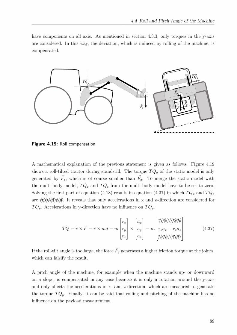
4.4 Roll and Pitch Angle of the Machine
have components on all axis. As mentioned in section 4.3.3, only torques in the y-axis
are considered. In this way, the deviation, which is induced by rolling of the machine, is
compensated.
� � � �
Figure 4.19: Roll compensation
A mathematical explanation of the previous statement is given as follows. Figure 4.19
shows a roll-tilted tractor during standstill. The torque TQy of the static model is only
generated by ~Fz, which is of course smaller than ~Fg. To merge the static model with
the multi-body model, TQx and TQz from the multi-body model have to be set to zero.
Solving the first part of equation (4.18) results in equation (4.37) in which TQx and TQz
are /////////crossed/////out. It reveals that only accelerations in x and z-direction are considered for
TQy. Accelerations in y-direction have no influence on TQy.
~TQ = ~r × ~F = ~r × m~a = m
rx
ry
rz
×
ax
ay
az
= m
ryaz − rzay/////////////
rzax − rxaz
rxay − ryax//////////////
(4.37)
If the roll-tilt angle is too large, the force ~Fy generates a higher friction torque at the joints,
which can falsify the result.
A pitch angle of the machine, for example when the machine stands up- or downward
on a slope, is compensated in any case because it is only a rotation around the y-axis
and only affects the accelerations in x- and z-direction, which are measured to generate
the torque TQy. Finally, it can be said that rolling and pitching of the machine has no
influence on the payload measurement.
89
4 Weighing Function
4.5 Implementation
This section describes the weighing algorithm as implemented at the prototype. To allow
plausibility checks during the early stage of development, the torque from the multi-body
model and from the static model need to be comparable. Hence, equation (4.30) and
equation (4.28) are transformed, in order to obtain comparable torque values from the
multi-body model and torque values from the static model for each joint J1 and J2. For
reasons of clarity, the vectors are not indexed with the respective coordinate system. In
this section, every vector is transformed to the same coordinate system, here to the boom
coordinate system K3. For instance,K4
↓ RK3
·~aBU is now written as ~aBU .
Subtracting equation (4.30) from equation (4.28) generates the following term:
0 = ~TQ1 − ~TQ2
+ [~rcogBM × (−mBM · ~aBM)] + [~rcogBU × (−mBU · ~aBU)]
+ [~rN × (−mBU · ~aBU)] + [~rcogL × (−mL · ~aL)]
+ [~rN × (−mL · ~aL)] − ΘBM ~ϕS3 − (ΘBU + ΘL) ~ϕS4
−[
[~rcogBU × (−mBU · ~aBU)] + [~rcogL × (−mL · ~aL)] − (ΘBU + ΘL) ~ϕS4
]
(4.38)
The previous equation is simplified to the following expression:
0 = ~TQ1 − ~TQ2 + [~rN × (−mL · ~aL)]
+
{
[~rcogBM × (−mBM · ~aBM)] + [~rcogBU × (−mBU · ~aBU)]
+ [~rN × (−mBU · ~aBU)] − ΘBM ~ϕS3 − (ΘBU + ΘL) ~ϕS4
}
−{
[~rcogBU × (−mBU · ~aBU)] − (ΘBU + ΘL) ~ϕS4
}
(4.39)
The terms in the curly brackets are replaced by the expressions ~TQ1 by acc and ~TQ2 by acc:
[~rN × (mL · ~aL)] = ~TQ1 − ~TQ2 +{
~TQ1 by acc
}
−{
~TQ2 by acc
}
(4.40)
The expressions ~TQ1 by acc and ~TQ2 by acc are obtained from the multi-body model. They
include all individual torques caused by every part of the front loader, such as cylinders or
links from the bucket linkage. An example of the different parts of the front loader with
90
4.5 Implementation
their center of gravity is shown in figure 4.14. ~TQ1 and ~TQ2 are replaced by
~TQ1 = − ~TQ1 meas
~TQ2 = − ~TQ2 meas
(4.41)
~TQ1 meas and ~TQ2 meas are calculated by the static model with measured cylinder forces.
The negative value is used to easily compare them to the torques of the multi-body model.
For example, ~TQ1 meas = ~TQ1 by acc or ~TQ2 meas = ~TQ2 by acc applies to a front loader without
payload.
4.5.1 Payload
The payload is calculated by solving equation (4.40) to mL. It is not possible to divide
two vectors by each other, but in case of a planar kinematic chain, like the front loader,
torque has only a y-component, hence, only the y-components are divided by each other.
mL =
[
− ~TQ1 meas + ~TQ2 meas + ~TQ1 by acc − ~TQ2 by acc
]
y[
~rN × ~aL
]
y
(4.42)
4.5.2 Simplifications
In the following, several further simplifications are described, that serve to ease the imple-
mentation at the tractor front loader.
4.5.2.1 Moments of Inertia
As mentioned in chapter 4.2.2.1, the accelerations ~ai are referenced to the center of gravity
of each part. Thus, the torque influence of the moment of inertia Θ is low compared to
other torque terms (cf. equation (4.39)). Hence, only the moments of inertia from big
parts, such as boom or tool carrier, are considered whereas moments of inertia of small
parts, for instance links of the bucket linkage, are not considered.
4.5.2.2 Oil Mass
The oil was drained before measuring the cylinder mass for the multi-body model. In
operation, the oil volume in the cylinders changes and, thereby, the mass of the cylinder
changes as well. Given that the cylinders are not too big, the oil mass in the cylinders is
not considered. In the reduced multi-body model (chapter 4.6.1) the oil mass is considered.
91
4 Weighing Function
4.5.2.3 Hoses
Flexible hoses are used to transfer the hydraulic power from the tractor to the cylinders
of the front loader. The hoses are fixed to the front loader and are bent to follow the
movements of the front loader. These bending forces influence the torques TQ1 at joint
J1 between chassis and boom and TQ2 at joint J2 between boom and bucket. Due to the
fact that the hoses are quite thin, the bending forces are low and not considered.
4.5.2.4 Relative Movements
An IMU is mounted at a given position. The output of the IMU is used to calculate the
acceleration at the center of gravity for each part as shown in chapter 2.6. In case of
a front loader, the parts are moving relative to each other. For instance, the bucket or
tool carrier moves relative to the boom, which causes Coriolis accelerations and further
rotational accelerations, as described in equation (2.22). Since relative movements are slow
compared to the overall movement, the front loader is treated as a rigid body and Coriolis
accelerations and further rotational accelerations are not considered for smaller parts. For
bigger parts, like the tool carrier or the payload, Coriolis acceleration and further rotational
accelerations must be considered. The IMU can be mounted anywhere at the tractor but
in order to reduce relative movements between mounting position and the relevant part as
well as to minimize deviations, the IMU is mounted at the boom (IMU S3).
4.5.2.5 Acceleration Sensor Position and Output
Chapter 2.6 describes how to transfer accelerations from one point to another. At a
rigid body, equation (4.43) calculates an acceleration ~a for any point P , measured at
IMU position S (cf. equation (2.20)). The distance between IMU and point P is given by
the vector ~rSP .
~a = ~r1P = ~r1S + ~ϕ2 ×(
~ϕ2 × [~rSP ])
+ ~ϕ2 × [~rSP ] (4.43)
If equation (4.43) is solved, it results in equation (4.44).
~a =
r1Sx
r1Sy////
r1Sz
+
ϕ2y(ϕ2x
rSPy− ϕ2y
rSPx) − ϕ2z
(ϕ2zrSPx
− ϕ2xrSPz
)
ϕ2z(ϕ2y
rSPz− ϕ2z
rSPy) − ϕ2x
(ϕ2xrSPy
− ϕ2yrSPx
)////////////////////////////////////////////////////////////
ϕ2x(ϕ2z
rSPx− ϕ2x
rSPz) − ϕ2y
(ϕ2yrSPz
− ϕ2zrSPy
)
+
ϕ2yrSPz
− ϕ2zrSPy
ϕ2zrSPx
− ϕ2xrSPz//////////////////////
ϕ2xrSPy
− ϕ2yrSPx
(4.44)
Forces in the y-direction are supported directly by the front loader joints. Hence, acceler-
ations in the y-direction have no influence and are not considered (/////////crossed/////out).
92
4.6 Optimized Model for Simple Parameter Identification
The IMU S3 used in this thesis has only three degrees of freedom. It measures accel-
erations in the x- and z-direction, rotational velocity, and rotational acceleration along the
y-axis. Therefore, ϕ2x, ϕ2z
and ϕ2x, ϕ2z
are not measured and set to zero. This influences
equation (4.44) and the terms marked with a dashed underline become zero:
~a =
r1Sx
0
r1Sz
+
ϕ2y(−ϕ2y
rSPx)
0
−ϕ2y(ϕ2y
rSPz)
+
ϕ2yrSPz
0
−ϕ2yrSPx
(4.45)
To minimize the deviations caused by the missing or disturbed angular velocities and ac-
celerations, the vector ~rSP has to be minimized. This requires a position of the acceleration
sensor close to the center of gravity. The multi-body model has several centers of grav-
ity. Because of this, the IMU position should be chosen between the center of gravity of
the biggest part, usually the boom, and the estimated center of gravity of the payload.
In chapter 4.6.1, all centers of gravity are summarized in a single one. This determines
the IMU position between the summarized center of gravity and the bucket where the
estimated center of gravity of the payload is located.
4.6 Optimized Model for Simple Parameter Identification
One major goal of this thesis is to avoid the extensive calibration process of current mobile
scales, which makes it difficult to install them in serial production. However, the op-
portunity must be provided to adjust the weighing system to compensate manufacturing
tolerances or front loader structure changes. For example, if an additional part is mounted
to the boom, its mass changes and has to be considered in the payload measurement, which
requires to tune or to re-calibrate the loader scale.
The full multi-body model as described in section 4.2 requires all masses, center of gravity
positions and inertias of each part. It is very labor-intensive and time-consuming to iden-
tify these parameters. In this thesis, a standard series front loader is taken apart as shown
in figure A.4 and for every part the mass, moment of inertia, and center of gravity position
is measured as described in section 2.7 and section 2.8. In serial production, these param-
eters are subject to tolerance and they will vary for each loader, which makes it necessary
to identify these parameters for each loader. This is not feasible for larger productions.
Hence, the multi-body model needs to be modified in a way that the parameters can be
easily identified. To achieve this, the approach of the reduced multi-body model and its
parameter identification is discussed in the following sections.
93
4 Weighing Function
4.6.1 Reduced Multi-Body Model
A reduced multi-body model is developed, whose parameters can be measured by a short
calibration procedure on each front loader. The full multi-body model is still used as a
reference for later comparison. On the basis of the section Payload Calculation, a closer
look at equation (4.32) reveals that many parameters are constant. These parameters are
marked with an underline in equation (4.46):
mL ·[
~rN × (K4
↓ RK3
·~aL)
]
=
[
~TQ1 − ~TQ2 − mBM · [~rcogBM × ~aBM ] − mBU · [~rN × (K4
↓ RK3
·~aBU)] − ΘBM ~ϕS3
] (4.46)
The masses and the respective center of gravity vectors remain constant. The masses
connected to the second joint, like mBU only depend on vector ~rN . Thus, it is obvious to
sum up all single masses to obtain mSum and to merge the centers of gravity to receive
~rcogSum. As mentioned in 4.5.2.1, the influence of the moment of inertia is low as long
as the acceleration ~aSum is referenced to the center of gravity. Therefore, all moments of
inertia Θi of all parts are combined and replaced by a beam with the length and height of
the front loader structure and with the equivalent mass of all parts (cf. equation (A.13)).
ΘSum =1
12(mSum − mBU)
(
(lengthBM)2 + (heightBM)2)
(4.47)
The weighing algorithm is independent of the moment of inertia of parts connected to the
second joint J2. For example, the moment of inertia of the payload ΘL and of the bucket
ΘBU do not appear in equation (4.46). Their effects are only measurable in ~TQ1 and ~TQ2.
For this reason, in order to calculate ΘSum, the mass of the bucket mBU must be subtracted
from mSum. With these assumptions, equation (4.46) turns into the following equation:
mL ·[
~rN × (K4
↓ RK3
·~aL)
]
= ~TQ1 − ~TQ2 − mSum · [~rcogSum × ~aSum] − ΘSum ~ϕS3 (4.48)
Figure 4.20 illustrates equation (4.48) for a front loader without payload, mL = 0. In figure
4.20 a) to c) the generated torque of mBU at the first joint is substituted by removing the
lever ~rcogBU and adding a torque ~TQ2. From now on, the generated torque of mBU depends
only on vector ~rN . Given that vector ~rN belongs to the boom and is constant and that
vector ~rcogBM is constant, the centers of gravity can be merged to receive ~rcogSum. The
moment of inertia is implied by the square box as shown in figure 4.20 d). The torque~TQ2 is obtained by the static model as described in chapter 4.1.3.2 and, finally, equation
(4.48) is solved to receive the payload mL as described in chapter 4.3.3.
94
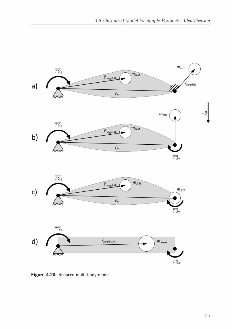
4.6 Optimized Model for Simple Parameter Identification
� � ��
− � �
� � �� �
� � �� �
� �
����
����
���� � � ��a)
b)
c)
d)
Figure 4.20: Reduced multi-body model
95
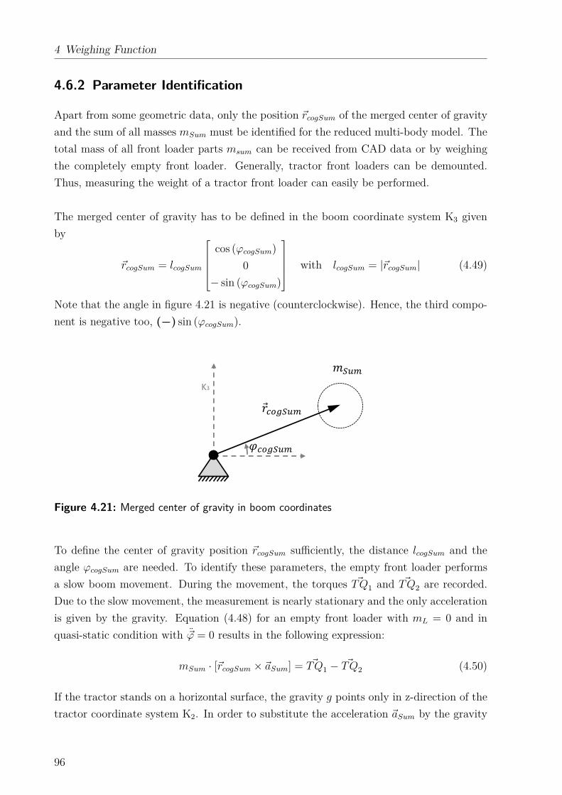
4 Weighing Function
4.6.2 Parameter Identification
Apart from some geometric data, only the position ~rcogSum of the merged center of gravity
and the sum of all masses mSum must be identified for the reduced multi-body model. The
total mass of all front loader parts msum can be received from CAD data or by weighing
the completely empty front loader. Generally, tractor front loaders can be demounted.
Thus, measuring the weight of a tractor front loader can easily be performed.
The merged center of gravity has to be defined in the boom coordinate system K3 given
by
~rcogSum = lcogSum
cos (ϕcogSum)
0
− sin (ϕcogSum)
with lcogSum = |~rcogSum| (4.49)
Note that the angle in figure 4.21 is negative (counterclockwise). Hence, the third compo-
nent is negative too, (−) sin (ϕcogSum).
K3 � �� �
Figure 4.21: Merged center of gravity in boom coordinates
To define the center of gravity position ~rcogSum sufficiently, the distance lcogSum and the
angle ϕcogSum are needed. To identify these parameters, the empty front loader performs
a slow boom movement. During the movement, the torques ~TQ1 and ~TQ2 are recorded.
Due to the slow movement, the measurement is nearly stationary and the only acceleration
is given by the gravity. Equation (4.48) for an empty front loader with mL = 0 and in
quasi-static condition with ~ϕ = 0 results in the following expression:
mSum · [~rcogSum × ~aSum] = ~TQ1 − ~TQ2 (4.50)
If the tractor stands on a horizontal surface, the gravity g points only in z-direction of the
tractor coordinate system K2. In order to substitute the acceleration ~aSum by the gravity
96
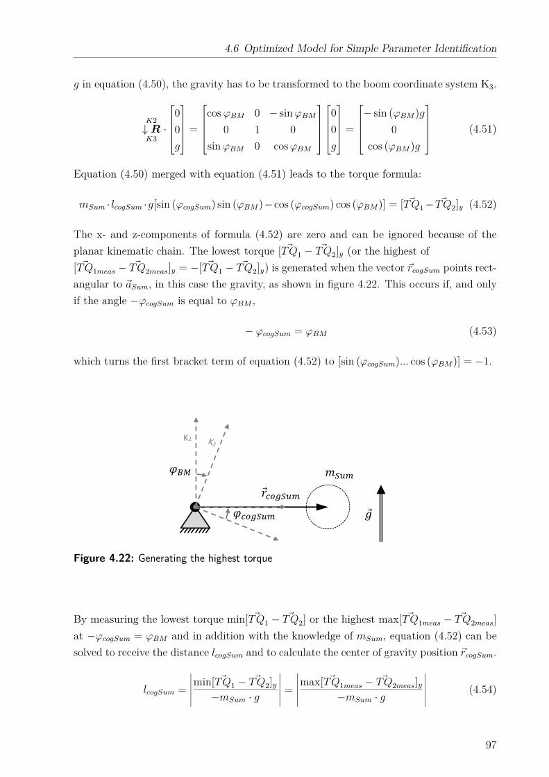
4.6 Optimized Model for Simple Parameter Identification
g in equation (4.50), the gravity has to be transformed to the boom coordinate system K3.
K2
↓ RK3
·
0
0
g
=
cos ϕBM 0 − sin ϕBM
0 1 0
sin ϕBM 0 cos ϕBM
0
0
g
=
− sin (ϕBM)g
0
cos (ϕBM)g
(4.51)
Equation (4.50) merged with equation (4.51) leads to the torque formula:
mSum · lcogSum ·g[sin (ϕcogSum) sin (ϕBM)−cos (ϕcogSum) cos (ϕBM)] = [ ~TQ1 − ~TQ2]y (4.52)
The x- and z-components of formula (4.52) are zero and can be ignored because of the
planar kinematic chain. The lowest torque [ ~TQ1 − ~TQ2]y (or the highest of
[ ~TQ1meas − ~TQ2meas]y = −[ ~TQ1 − ~TQ2]y) is generated when the vector ~rcogSum points rect-
angular to ~aSum, in this case the gravity, as shown in figure 4.22. This occurs if, and only
if the angle −ϕcogSum is equal to ϕBM ,
− ϕcogSum = ϕBM (4.53)
which turns the first bracket term of equation (4.52) to [sin (ϕcogSum)... cos (ϕBM)] = −1.
� �� �
K2
����
Figure 4.22: Generating the highest torque
By measuring the lowest torque min[ ~TQ1 − ~TQ2] or the highest max[ ~TQ1meas − ~TQ2meas]
at −ϕcogSum = ϕBM and in addition with the knowledge of mSum, equation (4.52) can be
solved to receive the distance lcogSum and to calculate the center of gravity position ~rcogSum.
lcogSum =
∣
∣
∣
∣
∣
∣
min[ ~TQ1 − ~TQ2]y−mSum · g
∣
∣
∣
∣
∣
∣
=
∣
∣
∣
∣
∣
∣
max[ ~TQ1meas − ~TQ2meas]y−mSum · g
∣
∣
∣
∣
∣
∣
(4.54)
97
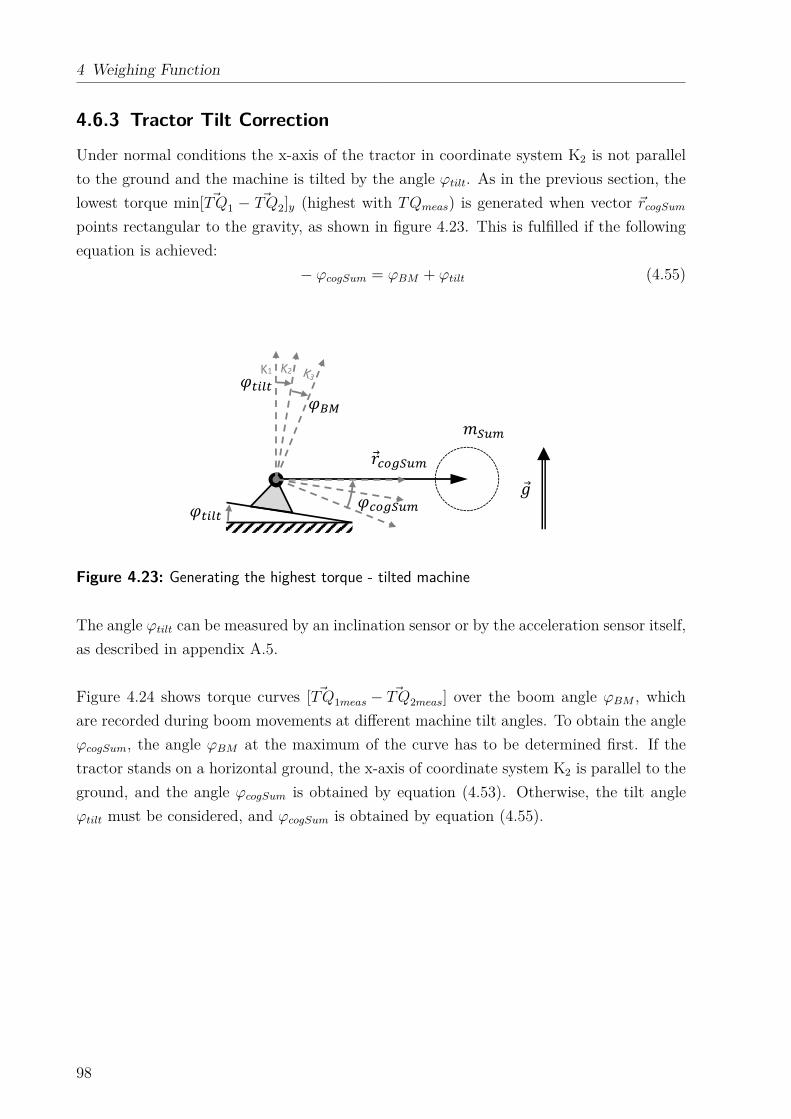
4 Weighing Function
4.6.3 Tractor Tilt Correction
Under normal conditions the x-axis of the tractor in coordinate system K2 is not parallel
to the ground and the machine is tilted by the angle ϕtilt. As in the previous section, the
lowest torque min[ ~TQ1 − ~TQ2]y (highest with TQmeas) is generated when vector ~rcogSum
points rectangular to the gravity, as shown in figure 4.23. This is fulfilled if the following
equation is achieved:
− ϕcogSum = ϕBM + ϕtilt (4.55)
� �� � ����K1
� �
� �
Figure 4.23: Generating the highest torque - tilted machine
The angle ϕtilt can be measured by an inclination sensor or by the acceleration sensor itself,
as described in appendix A.5.
Figure 4.24 shows torque curves [ ~TQ1meas − ~TQ2meas] over the boom angle ϕBM , which
are recorded during boom movements at different machine tilt angles. To obtain the angle
ϕcogSum, the angle ϕBM at the maximum of the curve has to be determined first. If the
tractor stands on a horizontal ground, the x-axis of coordinate system K2 is parallel to the
ground, and the angle ϕcogSum is obtained by equation (4.53). Otherwise, the tilt angle
ϕtilt must be considered, and ϕcogSum is obtained by equation (4.55).
98
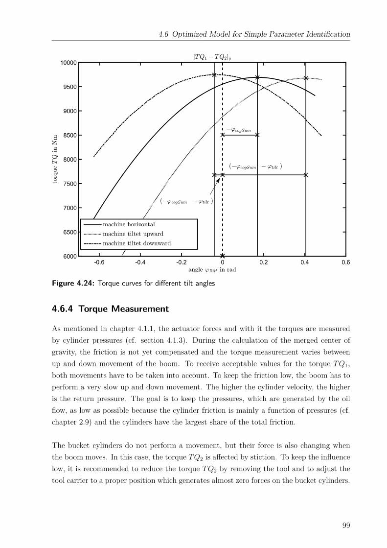
4.6 Optimized Model for Simple Parameter Identification
-0.6 -0.4 -0.2 0 0.2 0.4 0.6
6000
6500
7000
7500
8000
8500
9000
9500
10000
Figure 4.24: Torque curves for different tilt angles
4.6.4 Torque Measurement
As mentioned in chapter 4.1.1, the actuator forces and with it the torques are measured
by cylinder pressures (cf. section 4.1.3). During the calculation of the merged center of
gravity, the friction is not yet compensated and the torque measurement varies between
up and down movement of the boom. To receive acceptable values for the torque TQ1,
both movements have to be taken into account. To keep the friction low, the boom has to
perform a very slow up and down movement. The higher the cylinder velocity, the higher
is the return pressure. The goal is to keep the pressures, which are generated by the oil
flow, as low as possible because the cylinder friction is mainly a function of pressures (cf.
chapter 2.9) and the cylinders have the largest share of the total friction.
The bucket cylinders do not perform a movement, but their force is also changing when
the boom moves. In this case, the torque TQ2 is affected by stiction. To keep the influence
low, it is recommended to reduce the torque TQ2 by removing the tool and to adjust the
tool carrier to a proper position which generates almost zero forces on the bucket cylinders.
99
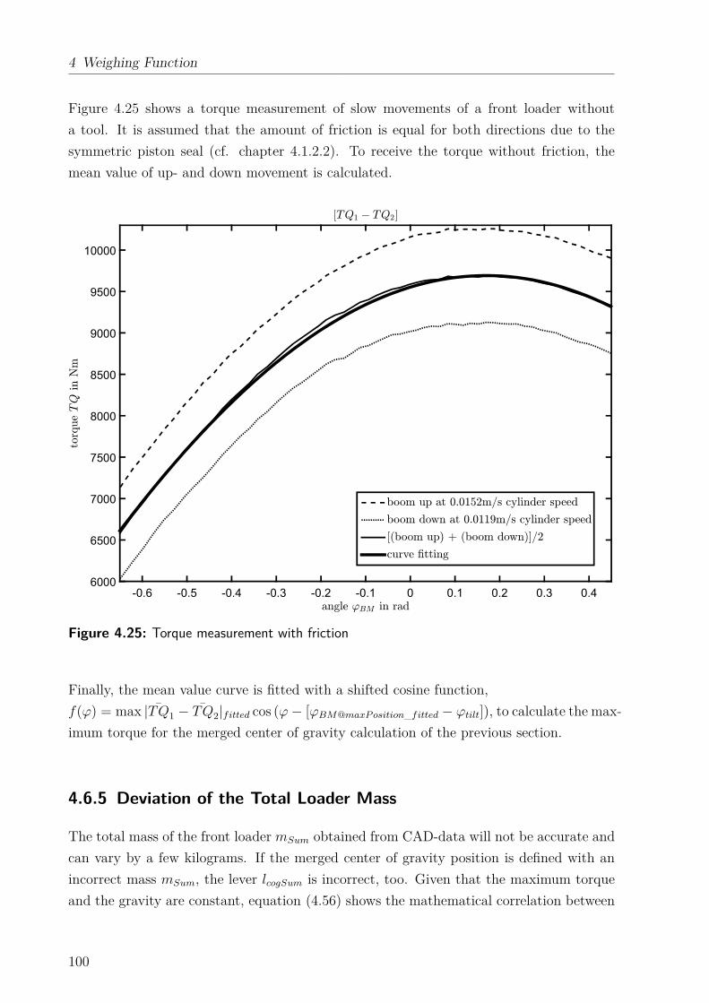
4 Weighing Function
Figure 4.25 shows a torque measurement of slow movements of a front loader without
a tool. It is assumed that the amount of friction is equal for both directions due to the
symmetric piston seal (cf. chapter 4.1.2.2). To receive the torque without friction, the
mean value of up- and down movement is calculated.
-0.6 -0.5 -0.4 -0.3 -0.2 -0.1 0 0.1 0.2 0.3 0.4
6000
6500
7000
7500
8000
8500
9000
9500
10000
Figure 4.25: Torque measurement with friction
Finally, the mean value curve is fitted with a shifted cosine function,
f(ϕ) = max | ¯TQ1 − ¯TQ2|fitted cos (ϕ − [ϕBM@maxP osition_fitted − ϕtilt]), to calculate the max-
imum torque for the merged center of gravity calculation of the previous section.
4.6.5 Deviation of the Total Loader Mass
The total mass of the front loader mSum obtained from CAD-data will not be accurate and
can vary by a few kilograms. If the merged center of gravity position is defined with an
incorrect mass mSum, the lever lcogSum is incorrect, too. Given that the maximum torque
and the gravity are constant, equation (4.56) shows the mathematical correlation between
100
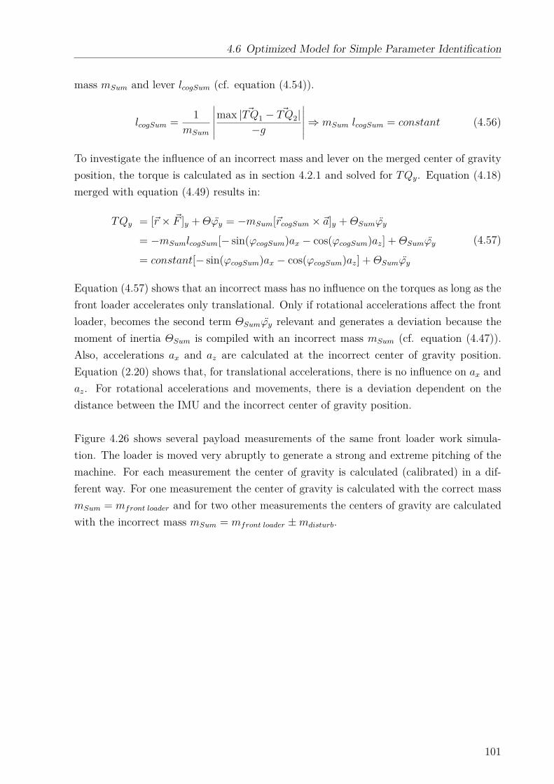
4.6 Optimized Model for Simple Parameter Identification
mass mSum and lever lcogSum (cf. equation (4.54)).
lcogSum =1
mSum
∣
∣
∣
∣
∣
∣
max | ~TQ1 − ~TQ2|−g
∣
∣
∣
∣
∣
∣
⇒ mSum lcogSum = constant (4.56)
To investigate the influence of an incorrect mass and lever on the merged center of gravity
position, the torque is calculated as in section 4.2.1 and solved for TQy. Equation (4.18)
merged with equation (4.49) results in:
TQy = [~r × ~F ]y + Θϕy = −mSum[~rcogSum × ~a]y + ΘSumϕy
= −mSumlcogSum[− sin(ϕcogSum)ax − cos(ϕcogSum)az] + ΘSumϕy
= constant[− sin(ϕcogSum)ax − cos(ϕcogSum)az] + ΘSumϕy
(4.57)
Equation (4.57) shows that an incorrect mass has no influence on the torques as long as the
front loader accelerates only translational. Only if rotational accelerations affect the front
loader, becomes the second term ΘSumϕy relevant and generates a deviation because the
moment of inertia ΘSum is compiled with an incorrect mass mSum (cf. equation (4.47)).
Also, accelerations ax and az are calculated at the incorrect center of gravity position.
Equation (2.20) shows that, for translational accelerations, there is no influence on ax and
az. For rotational accelerations and movements, there is a deviation dependent on the
distance between the IMU and the incorrect center of gravity position.
Figure 4.26 shows several payload measurements of the same front loader work simula-
tion. The loader is moved very abruptly to generate a strong and extreme pitching of the
machine. For each measurement the center of gravity is calculated (calibrated) in a dif-
ferent way. For one measurement the center of gravity is calculated with the correct mass
mSum = mfront loader and for two other measurements the centers of gravity are calculated
with the incorrect mass mSum = mfront loader ± mdisturb.
101
4 Weighing Function
800
850
900
950
1000
1050
1100
1150
65 70 75 80 85 90 95 100 105 110
-5
0
5
Figure 4.26: Payload measurement in extreme conditions with incorrect mSum and ~rcogSum
The greater the distance between sensor and incorrect center of gravity (~rcogSum − ~rS3),
the greater are the deviations at high boom pitch accelerations ϕS3_y. The measurement
in figure 4.26 was done in extreme conditions with high pitch rates, thus, the influence
of an incorrect mSum and ~rcogSum is low under normal conditions. Also, the obtained
mass mSum = mfront loader ± mdisturb from the CAD-model is generally more accurate, here
mdisturb = ±300kg is more than 50% of the front loader mass mfront loader = 541kg.
4.6.6 Deviation Compared to the Full Multi-Body Model
4.6.6.1 Merged Center of Gravity Position
The approach to merge the center of gravity positions to receive ~rcogSum is only valid for
rigidly mounted parts that are connected to the boom or tool carrier (BU). In this thesis,
however, this approach is also applied to parts that are not rigidly mounted to the boom
or tool carrier. Some parts change their center of gravity positions during the front loader
movements relative to the boom or tool carrier. For instance, the boom cylinders will
change their position relative to the boom during movements. For the reduced multi-body
102
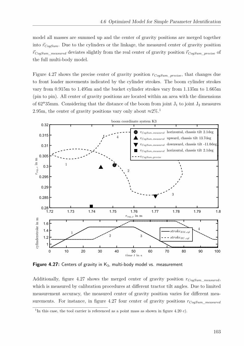
4.6 Optimized Model for Simple Parameter Identification
model all masses are summed up and the center of gravity positions are merged together
into ~rCogSum. Due to the cylinders or the linkage, the measured center of gravity position
~rCogSum_measured deviates slightly from the real center of gravity position ~rCogSum_precise of
the full multi-body model.
Figure 4.27 shows the precise center of gravity position rCogSum_precise, that changes due
to front loader movements indicated by the cylinder strokes. The boom cylinder strokes
vary from 0.915m to 1.495m and the bucket cylinder strokes vary from 1.135m to 1.665m
(pin to pin). All center of gravity positions are located within an area with the dimensions
of 62*35mm. Considering that the distance of the boom from joint J1 to joint J2 measures
2.95m, the center of gravity positions vary only about ≈2%.1
1.72 1.73 1.74 1.75 1.76 1.77 1.78 1.79 1.8
0.28
0.285
0.29
0.295
0.3
0.305
0.31
0.315
0.32
0 10 20 30 40 50 60 70 80 90 100
1
1.2
1.4
1.6
Figure 4.27: Centers of gravity in K3, multi-body model vs. measurement
Additionally, figure 4.27 shows the merged center of gravity position rCogSum_measured,
which is measured by calibration procedures at different tractor tilt angles. Due to limited
measurement accuracy, the measured center of gravity position varies for different mea-
surements. For instance, in figure 4.27 four center of gravity positions rCogSum_measured
1In this case, the tool carrier is referenced as a point mass as shown in figure 4.20 c).
103
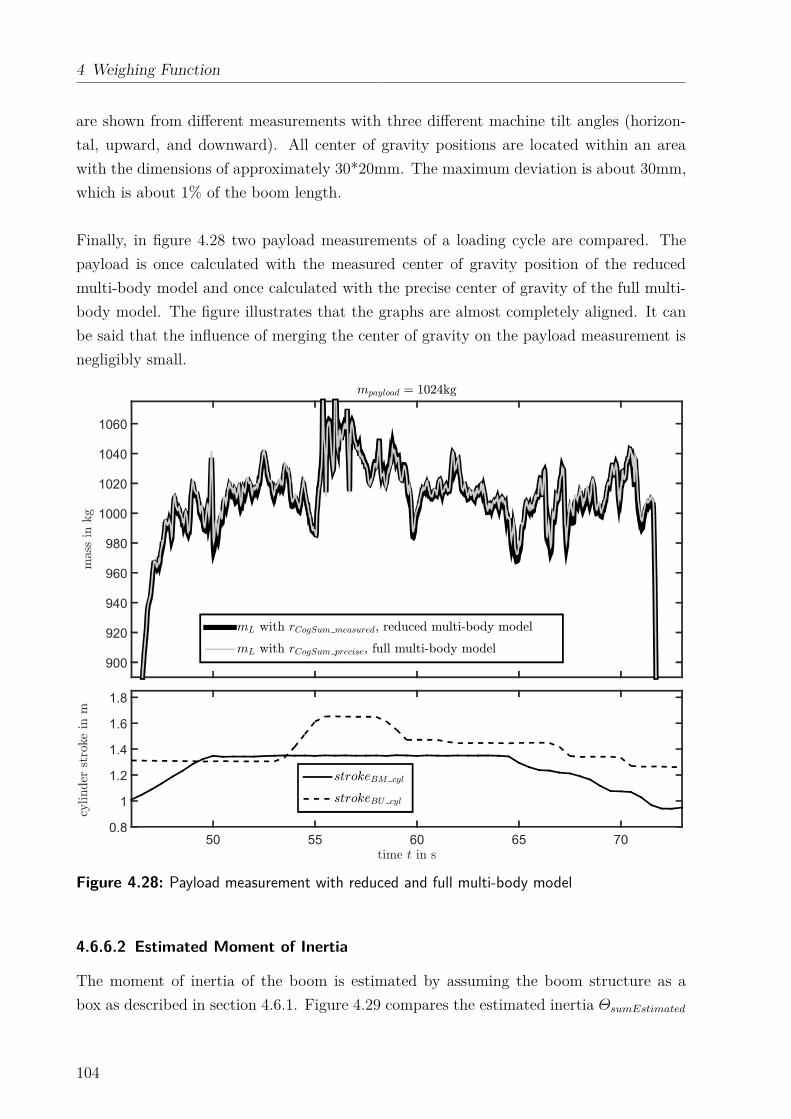
4 Weighing Function
are shown from different measurements with three different machine tilt angles (horizon-
tal, upward, and downward). All center of gravity positions are located within an area
with the dimensions of approximately 30*20mm. The maximum deviation is about 30mm,
which is about 1% of the boom length.
Finally, in figure 4.28 two payload measurements of a loading cycle are compared. The
payload is once calculated with the measured center of gravity position of the reduced
multi-body model and once calculated with the precise center of gravity of the full multi-
body model. The figure illustrates that the graphs are almost completely aligned. It can
be said that the influence of merging the center of gravity on the payload measurement is
negligibly small.
900
920
940
960
980
1000
1020
1040
1060
50 55 60 65 70
0.8
1
1.2
1.4
1.6
1.8
Figure 4.28: Payload measurement with reduced and full multi-body model
4.6.6.2 Estimated Moment of Inertia
The moment of inertia of the boom is estimated by assuming the boom structure as a
box as described in section 4.6.1. Figure 4.29 compares the estimated inertia ΘsumEstimated
104
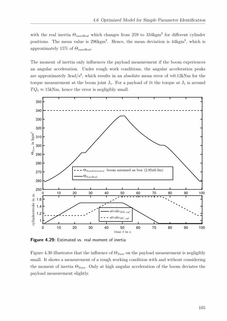
4.6 Optimized Model for Simple Parameter Identification
with the real inertia ΘsumReal which changes from 259 to 334kgm2 for different cylinder
positions. The mean value is 296kgm2. Hence, the mean deviation is 44kgm2, which is
approximately 15% of ΘsumReal.
The moment of inertia only influences the payload measurement if the boom experiences
an angular acceleration. Under rough work conditions, the angular acceleration peaks
are approximately 3rad/s2, which results in an absolute mean error of ≈0.12kNm for the
torque measurement at the boom joint J1. For a payload of 1t the torque at J1 is around
TQ1 ≈ 15kNm, hence the error is negligibly small.
0 10 20 30 40 50 60 70 80 90 100
250
260
270
280
290
300
310
320
330
340
350
0 10 20 30 40 50 60 70 80 90 100
1
1.2
1.4
1.6
Figure 4.29: Estimated vs. real moment of inertia
Figure 4.30 illustrates that the influence of ΘSum on the payload measurement is negligibly
small. It shows a measurement of a rough working condition with and without considering
the moment of inertia ΘSum. Only at high angular acceleration of the boom deviates the
payload measurement slightly.
105
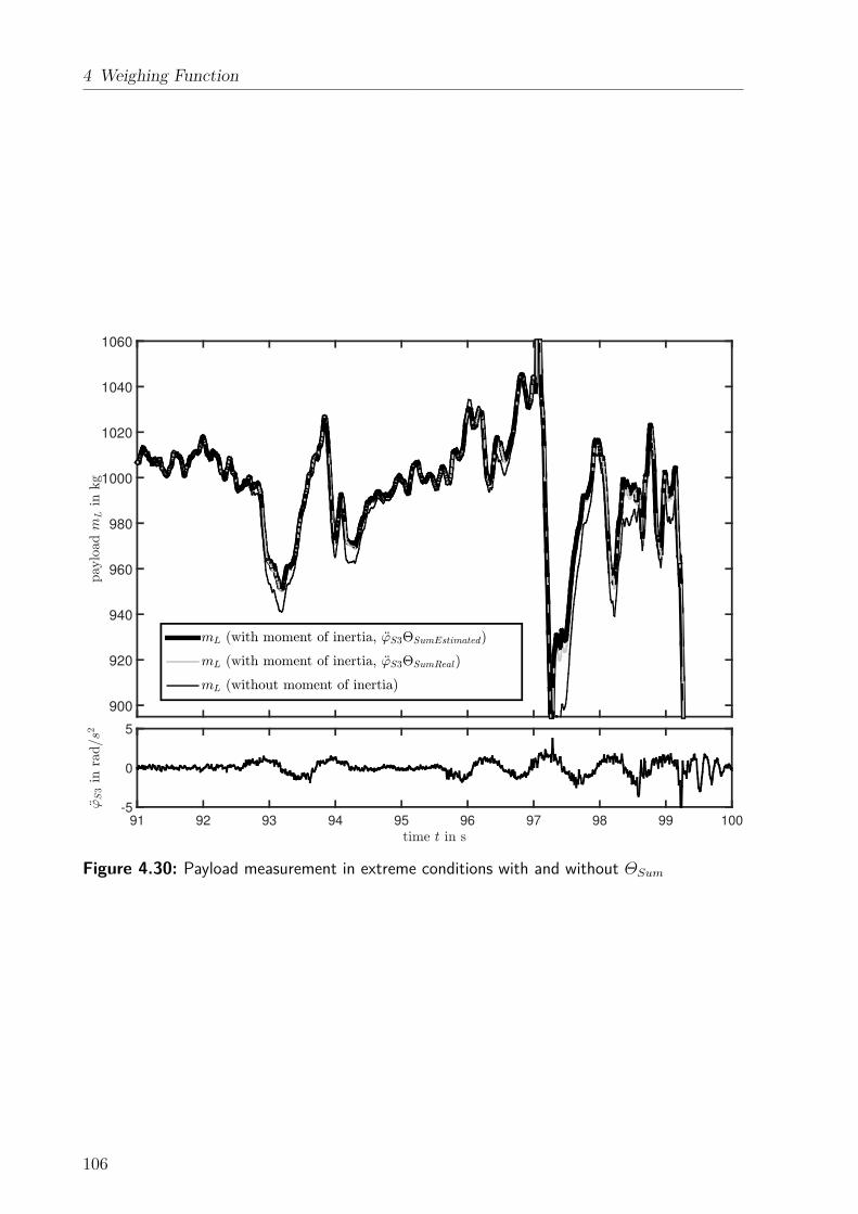
4 Weighing Function
900
920
940
960
980
1000
1020
1040
1060
91 92 93 94 95 96 97 98 99 100
-5
0
5
Figure 4.30: Payload measurement in extreme conditions with and without ΘSum
106
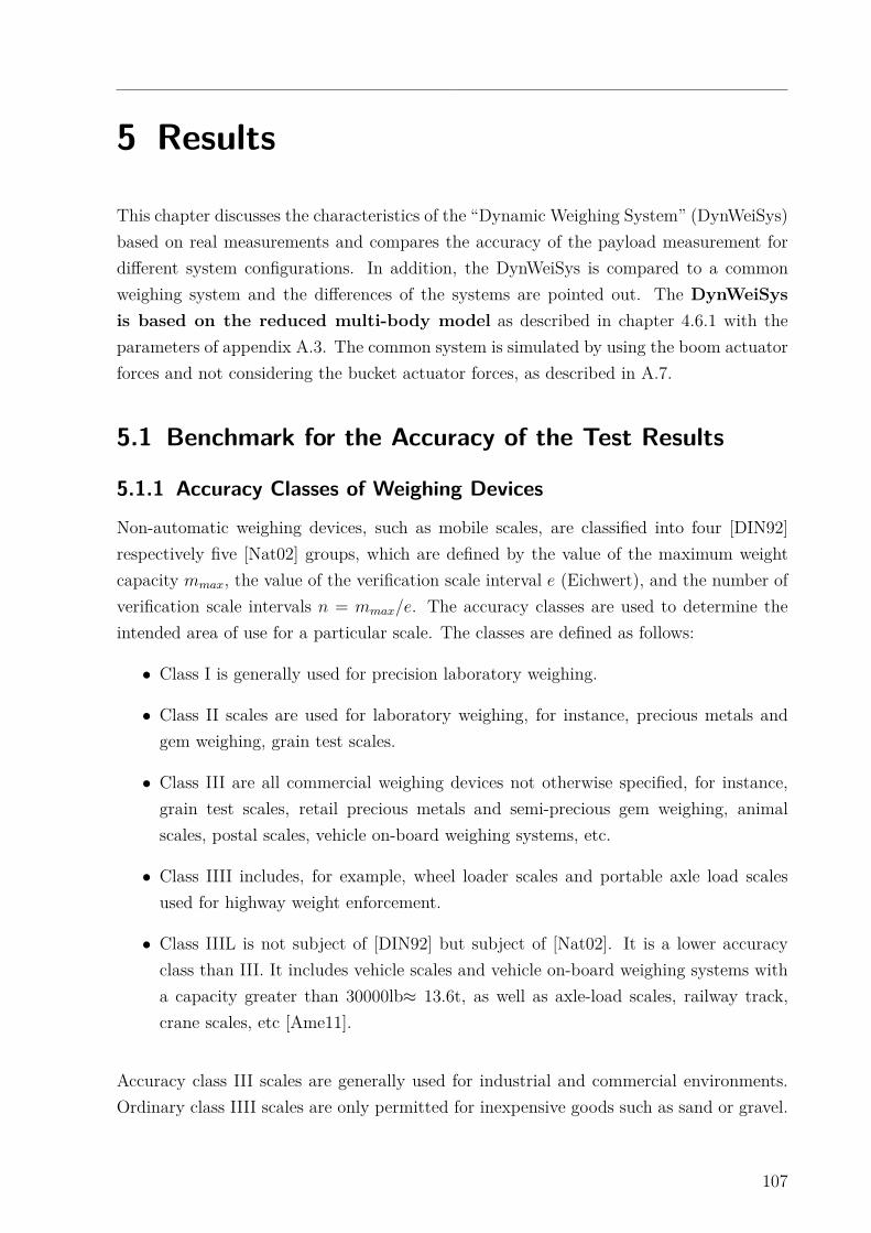
5 Results
This chapter discusses the characteristics of the “Dynamic Weighing System” (DynWeiSys)
based on real measurements and compares the accuracy of the payload measurement for
different system configurations. In addition, the DynWeiSys is compared to a common
weighing system and the differences of the systems are pointed out. The DynWeiSys
is based on the reduced multi-body model as described in chapter 4.6.1 with the
parameters of appendix A.3. The common system is simulated by using the boom actuator
forces and not considering the bucket actuator forces, as described in A.7.
5.1 Benchmark for the Accuracy of the Test Results
5.1.1 Accuracy Classes of Weighing Devices
Non-automatic weighing devices, such as mobile scales, are classified into four [DIN92]
respectively five [Nat02] groups, which are defined by the value of the maximum weight
capacity mmax, the value of the verification scale interval e (Eichwert), and the number of
verification scale intervals n = mmax/e. The accuracy classes are used to determine the
intended area of use for a particular scale. The classes are defined as follows:
• Class I is generally used for precision laboratory weighing.
• Class II scales are used for laboratory weighing, for instance, precious metals and
gem weighing, grain test scales.
• Class III are all commercial weighing devices not otherwise specified, for instance,
grain test scales, retail precious metals and semi-precious gem weighing, animal
scales, postal scales, vehicle on-board weighing systems, etc.
• Class IIII includes, for example, wheel loader scales and portable axle load scales
used for highway weight enforcement.
• Class IIIL is not subject of [DIN92] but subject of [Nat02]. It is a lower accuracy
class than III. It includes vehicle scales and vehicle on-board weighing systems with
a capacity greater than 30000lb≈ 13.6t, as well as axle-load scales, railway track,
crane scales, etc [Ame11].
Accuracy class III scales are generally used for industrial and commercial environments.
Ordinary class IIII scales are only permitted for inexpensive goods such as sand or gravel.
107
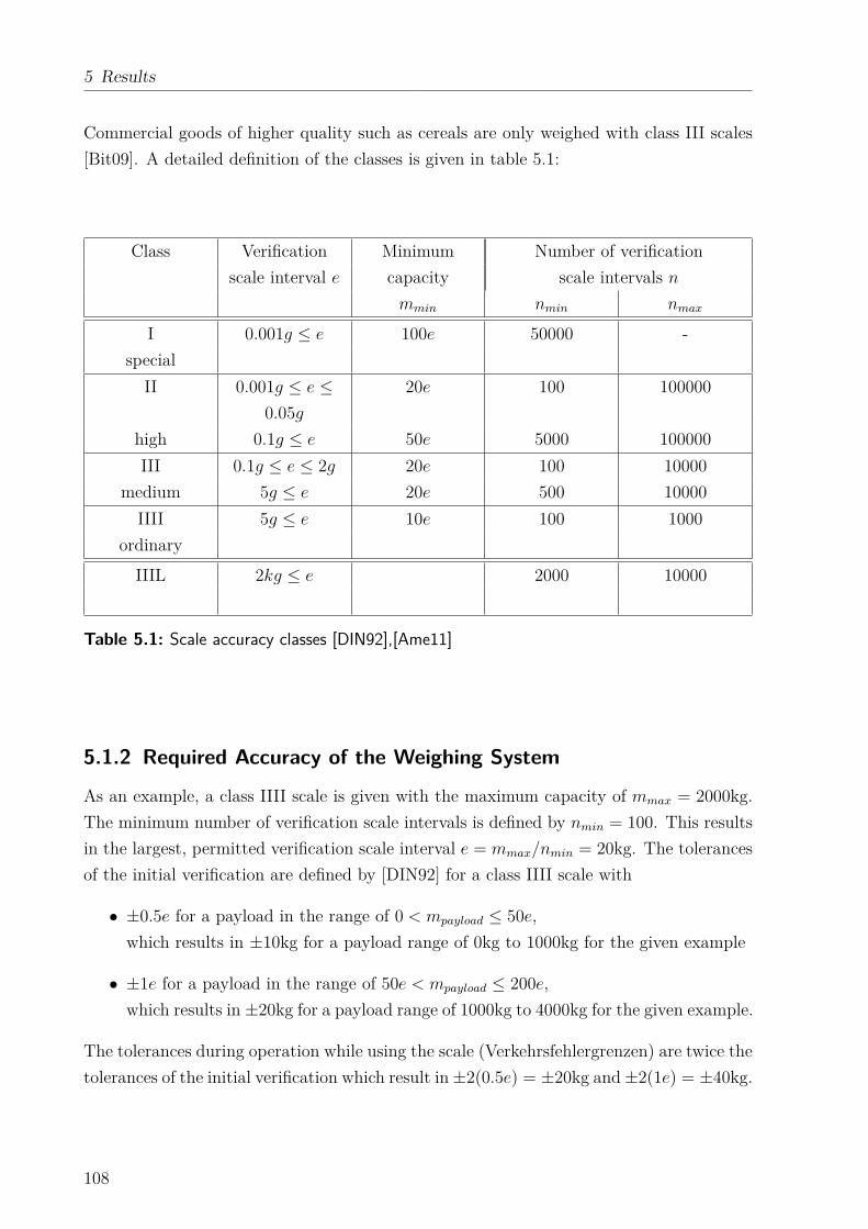
5 Results
Commercial goods of higher quality such as cereals are only weighed with class III scales
[Bit09]. A detailed definition of the classes is given in table 5.1:
Class Verification Minimum Number of verification
scale interval e capacity scale intervals n
mmin nmin nmax
I 0.001g ≤ e 100e 50000 -
special
II 0.001g ≤ e ≤0.05g
20e 100 100000
high 0.1g ≤ e 50e 5000 100000
III 0.1g ≤ e ≤ 2g 20e 100 10000
medium 5g ≤ e 20e 500 10000
IIII 5g ≤ e 10e 100 1000
ordinary
IIIL 2kg ≤ e 2000 10000
Table 5.1: Scale accuracy classes [DIN92],[Ame11]
5.1.2 Required Accuracy of the Weighing System
As an example, a class IIII scale is given with the maximum capacity of mmax = 2000kg.
The minimum number of verification scale intervals is defined by nmin = 100. This results
in the largest, permitted verification scale interval e = mmax/nmin = 20kg. The tolerances
of the initial verification are defined by [DIN92] for a class IIII scale with
• ±0.5e for a payload in the range of 0 < mpayload ≤ 50e,
which results in ±10kg for a payload range of 0kg to 1000kg for the given example
• ±1e for a payload in the range of 50e < mpayload ≤ 200e,
which results in ±20kg for a payload range of 1000kg to 4000kg for the given example.
The tolerances during operation while using the scale (Verkehrsfehlergrenzen) are twice the
tolerances of the initial verification which result in ±2(0.5e) = ±20kg and ±2(1e) = ±40kg.
108
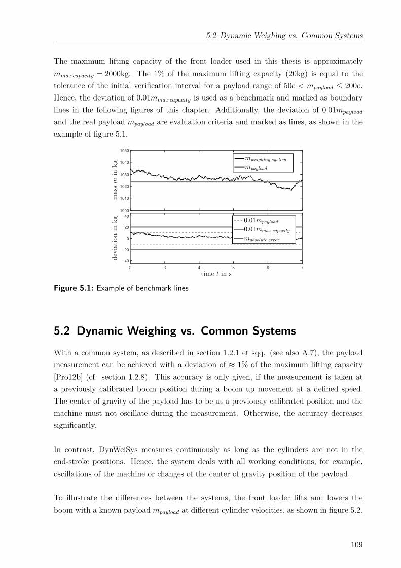
5.2 Dynamic Weighing vs. Common Systems
The maximum lifting capacity of the front loader used in this thesis is approximately
mmax capacity = 2000kg. The 1% of the maximum lifting capacity (20kg) is equal to the
tolerance of the initial verification interval for a payload range of 50e < mpayload ≤ 200e.
Hence, the deviation of 0.01mmax capacity is used as a benchmark and marked as boundary
lines in the following figures of this chapter. Additionally, the deviation of 0.01mpayload
and the real payload mpayload are evaluation criteria and marked as lines, as shown in the
example of figure 5.1.
1000
1010
1020
1030
1040
1050
2 3 4 5 6 7
-40
-20
0
20
40
Figure 5.1: Example of benchmark lines
5.2 Dynamic Weighing vs. Common Systems
With a common system, as described in section 1.2.1 et sqq. (see also A.7), the payload
measurement can be achieved with a deviation of ≈ 1% of the maximum lifting capacity
[Pro12b] (cf. section 1.2.8). This accuracy is only given, if the measurement is taken at
a previously calibrated boom position during a boom up movement at a defined speed.
The center of gravity of the payload has to be at a previously calibrated position and the
machine must not oscillate during the measurement. Otherwise, the accuracy decreases
significantly.
In contrast, DynWeiSys measures continuously as long as the cylinders are not in the
end-stroke positions. Hence, the system deals with all working conditions, for example,
oscillations of the machine or changes of the center of gravity position of the payload.
To illustrate the differences between the systems, the front loader lifts and lowers the
boom with a known payload mpayload at different cylinder velocities, as shown in figure 5.2.
109
5 Results
During the measurement, the bucket cylinders do not move in order to keep the center of
gravity position of the payload constant relatively to the boom.
�
Figure 5.2: Test configuration 1: Lifting and lowering of the boom with a constant bucketcylinder position
Figure 5.3 shows a measurement of test configuration 1. At the top of figure 5.3 the
payload readings of both systems are shown, which are displayed as mass over the time.
The common system (mcommon) takes the payload measurement only at a specific cylinder
stroke while the DynWeigSys (mDynW eiSys) measures continuously. The middle part of
figure 5.3 shows the absolute deviation over the time and the ±1%-boundary with respect
to the maximum lifting capacity and with respect to mpayload. The measurement of the
common system deviates strongly in different boom positions. Hence, the measurement
is only taken at a certain boom cylinder stroke during the lifting of the boom. The
deviation of the DynWeiSys is almost in the ±1%-boundary, regardless of the boom position
and movement. Deviations higher than 1% occur occasionally while lowering the boom.
The deviations are effected by inaccuracies of the friction model. The common system is
optimized for a boom up-movement at a specified actuator velocity. If the velocity or the
direction of movement changes, the payload measurement deviates due to changing friction
influences.
110
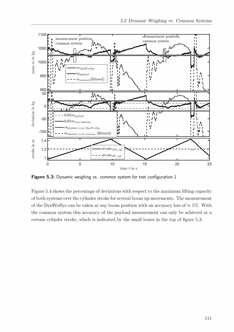
5.2 Dynamic Weighing vs. Common Systems
900
950
1000
1050
1100
-100
-50
0
50
0 5 10 15 20 25
1
1.2
1.4
Figure 5.3: Dynamic weighing vs. common system for test configuration 1
Figure 5.4 shows the percentage of deviations with respect to the maximum lifting capacity
of both systems over the cylinder stroke for several boom up-movements. The measurement
of the DynWeiSys can be taken at any boom position with an accuracy loss of ≈ 1%. With
the common system this accuracy of the payload measurement can only be achieved at a
certain cylinder stroke, which is indicated by the small boxes in the top of figure 5.3.
111
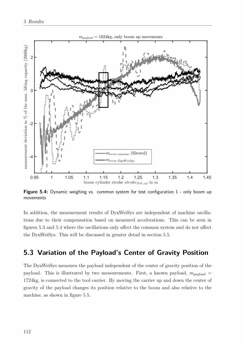
5 Results
0.95 1 1.05 1.1 1.15 1.2 1.25 1.3 1.35 1.4 1.45
-4
-2
0
2
Figure 5.4: Dynamic weighing vs. common system for test configuration 1 - only boom upmovements
In addition, the measurement results of DynWeiSys are independent of machine oscilla-
tions due to their compensation based on measured accelerations. This can be seen in
figures 5.3 and 5.4 where the oscillations only affect the common system and do not affect
the DynWeiSys. This will be discussed in greater detail in section 5.5.
5.3 Variation of the Payload’s Center of Gravity Position
The DynWeiSys measures the payload independent of the center of gravity position of the
payload. This is illustrated by two measurements. First, a known payload, mpayload =
1724kg, is connected to the tool carrier. By moving the carrier up and down the center of
gravity of the payload changes its position relative to the boom and also relative to the
machine, as shown in figure 5.5.
112
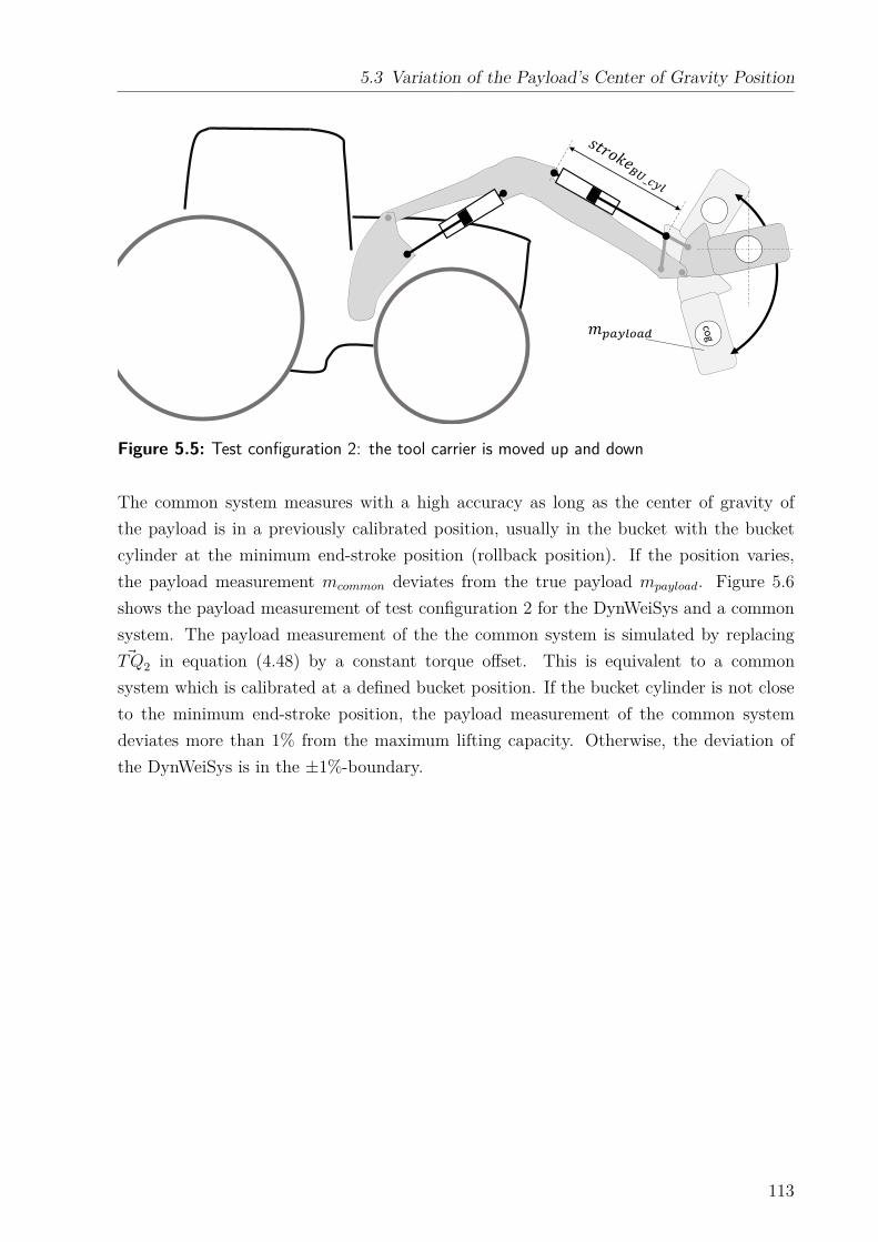
5.3 Variation of the Payload’s Center of Gravity Position
�
Figure 5.5: Test configuration 2: the tool carrier is moved up and down
The common system measures with a high accuracy as long as the center of gravity of
the payload is in a previously calibrated position, usually in the bucket with the bucket
cylinder at the minimum end-stroke position (rollback position). If the position varies,
the payload measurement mcommon deviates from the true payload mpayload. Figure 5.6
shows the payload measurement of test configuration 2 for the DynWeiSys and a common
system. The payload measurement of the the common system is simulated by replacing~TQ2 in equation (4.48) by a constant torque offset. This is equivalent to a common
system which is calibrated at a defined bucket position. If the bucket cylinder is not close
to the minimum end-stroke position, the payload measurement of the common system
deviates more than 1% from the maximum lifting capacity. Otherwise, the deviation of
the DynWeiSys is in the ±1%-boundary.
113
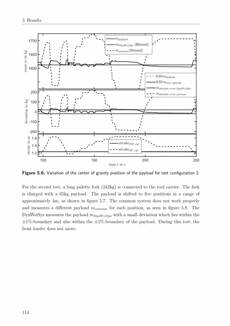
5 Results
1600
1650
1700
-200
-100
0
100
200
100 150 200 250
1.2
1.4
1.6
Figure 5.6: Variation of the center of gravity position of the payload for test configuration 2
For the second test, a long palette fork (242kg) is connected to the tool carrier. The fork
is charged with a 65kg payload. The payload is shifted to five positions in a range of
approximately 4m, as shown in figure 5.7. The common system does not work properly
and measures a different payload mcommon for each position, as seen in figure 5.8. The
DynWeiSys measures the payload mDynW eiSys with a small deviation which lies within the
±1%-boundary and also within the ±1%-boundary of the payload. During this test, the
front loader does not move.
114
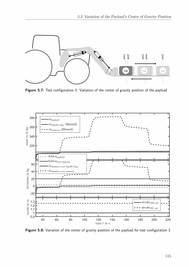
5.3 Variation of the Payload’s Center of Gravity Position
cogcog cog cogcog
po
s1
po
s5
po
s2
po
s4
po
s3
Figure 5.7: Test configuration 3: Variation of the center of gravity position of the payload
320
340
360
380
-20
0
20
40
60
40 60 80 100 120 140 160 180 200 2200,9
1
1,1
1,2
1,3
Figure 5.8: Variation of the center of gravity position of the payload for test configuration 3
115
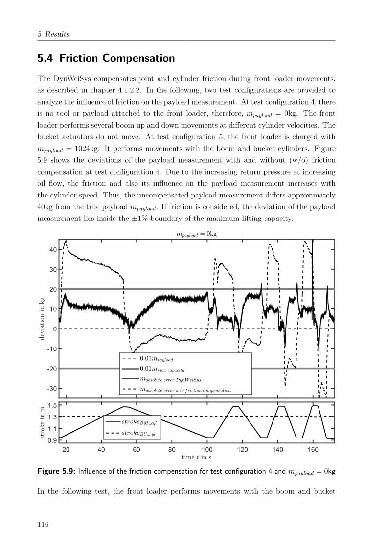
5 Results
5.4 Friction Compensation
The DynWeiSys compensates joint and cylinder friction during front loader movements,
as described in chapter 4.1.2.2. In the following, two test configurations are provided to
analyze the influence of friction on the payload measurement. At test configuration 4, there
is no tool or payload attached to the front loader, therefore, mpayload = 0kg. The front
loader performs several boom up and down movements at different cylinder velocities. The
bucket actuators do not move. At test configuration 5, the front loader is charged with
mpayload = 1024kg. It performs movements with the boom and bucket cylinders. Figure
5.9 shows the deviations of the payload measurement with and without (w/o) friction
compensation at test configuration 4. Due to the increasing return pressure at increasing
oil flow, the friction and also its influence on the payload measurement increases with
the cylinder speed. Thus, the uncompensated payload measurement differs approximately
40kg from the true payload mpayload. If friction is considered, the deviation of the payload
measurement lies inside the ±1%-boundary of the maximum lifting capacity.
-30
-20
-10
0
10
20
30
40
20 40 60 80 100 120 140 160
0.9
1.1
1.3
1.5
Figure 5.9: Influence of the friction compensation for test configuration 4 and mpayload = 0kg
In the following test, the front loader performs movements with the boom and bucket
116
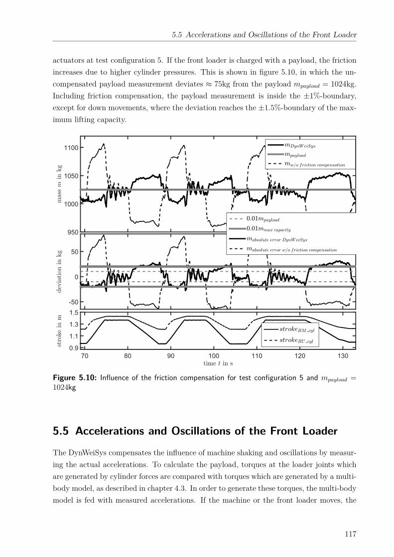
5.5 Accelerations and Oscillations of the Front Loader
actuators at test configuration 5. If the front loader is charged with a payload, the friction
increases due to higher cylinder pressures. This is shown in figure 5.10, in which the un-
compensated payload measurement deviates ≈ 75kg from the payload mpayload = 1024kg.
Including friction compensation, the payload measurement is inside the ±1%-boundary,
except for down movements, where the deviation reaches the ±1.5%-boundary of the max-
imum lifting capacity.
950
1000
1050
1100
-50
0
50
70 80 90 100 110 120 130
0.9
1.1
1.3
1.5
Figure 5.10: Influence of the friction compensation for test configuration 5 and mpayload =1024kg
5.5 Accelerations and Oscillations of the Front Loader
The DynWeiSys compensates the influence of machine shaking and oscillations by measur-
ing the actual accelerations. To calculate the payload, torques at the loader joints which
are generated by cylinder forces are compared with torques which are generated by a multi-
body model, as described in chapter 4.3. In order to generate these torques, the multi-body
model is fed with measured accelerations. If the machine or the front loader moves, the
117
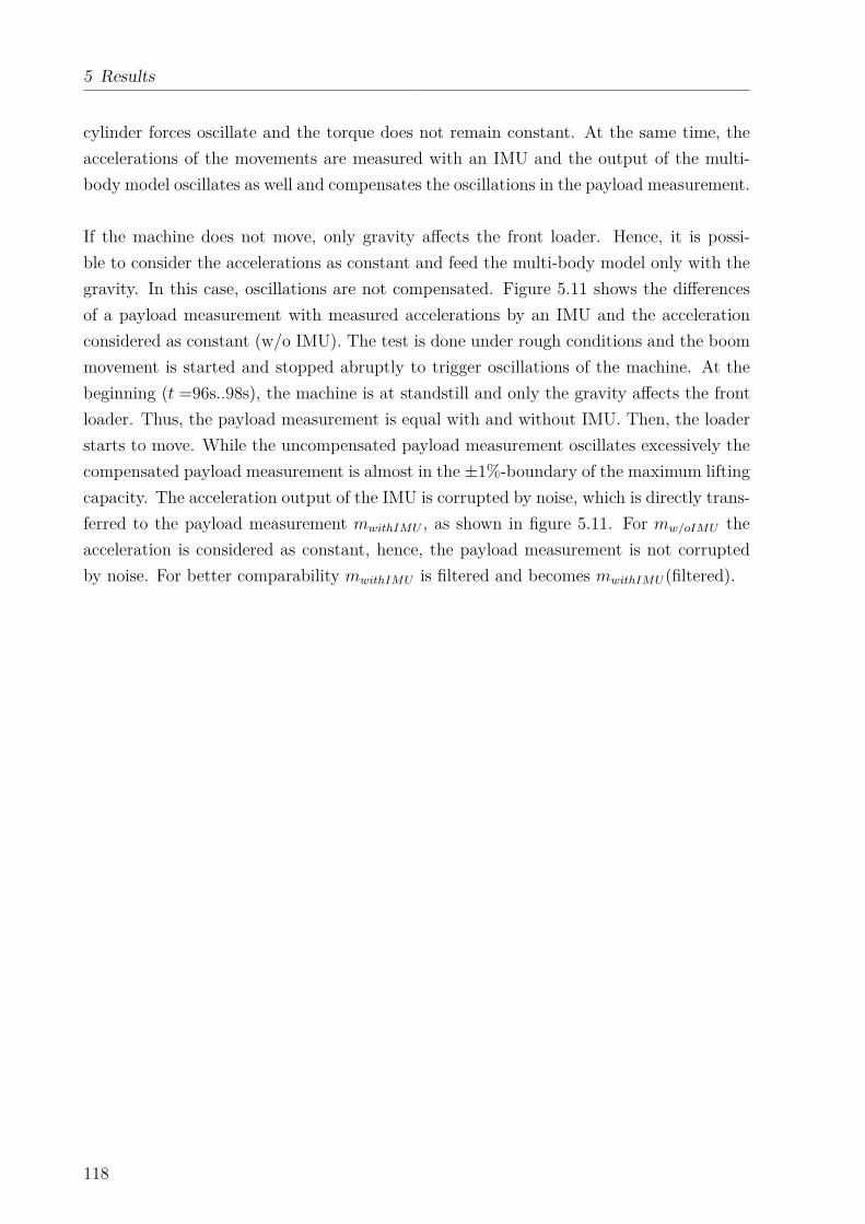
5 Results
cylinder forces oscillate and the torque does not remain constant. At the same time, the
accelerations of the movements are measured with an IMU and the output of the multi-
body model oscillates as well and compensates the oscillations in the payload measurement.
If the machine does not move, only gravity affects the front loader. Hence, it is possi-
ble to consider the accelerations as constant and feed the multi-body model only with the
gravity. In this case, oscillations are not compensated. Figure 5.11 shows the differences
of a payload measurement with measured accelerations by an IMU and the acceleration
considered as constant (w/o IMU). The test is done under rough conditions and the boom
movement is started and stopped abruptly to trigger oscillations of the machine. At the
beginning (t =96s..98s), the machine is at standstill and only the gravity affects the front
loader. Thus, the payload measurement is equal with and without IMU. Then, the loader
starts to move. While the uncompensated payload measurement oscillates excessively the
compensated payload measurement is almost in the ±1%-boundary of the maximum lifting
capacity. The acceleration output of the IMU is corrupted by noise, which is directly trans-
ferred to the payload measurement mwithIMU , as shown in figure 5.11. For mw/oIMU the
acceleration is considered as constant, hence, the payload measurement is not corrupted
by noise. For better comparability mwithIMU is filtered and becomes mwithIMU(filtered).
118
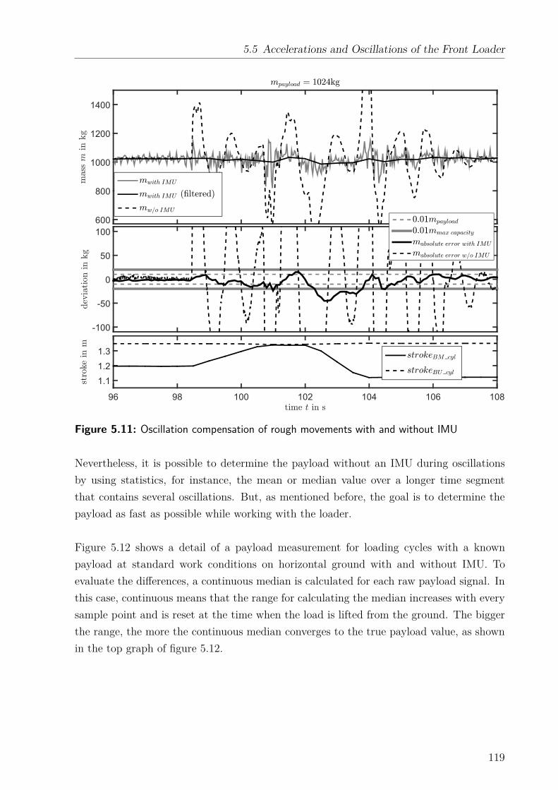
5.5 Accelerations and Oscillations of the Front Loader
600
800
1000
1200
1400
-100
-50
0
50
100
96 98 100 102 104 106 108
1.1
1.2
1.3
Figure 5.11: Oscillation compensation of rough movements with and without IMU
Nevertheless, it is possible to determine the payload without an IMU during oscillations
by using statistics, for instance, the mean or median value over a longer time segment
that contains several oscillations. But, as mentioned before, the goal is to determine the
payload as fast as possible while working with the loader.
Figure 5.12 shows a detail of a payload measurement for loading cycles with a known
payload at standard work conditions on horizontal ground with and without IMU. To
evaluate the differences, a continuous median is calculated for each raw payload signal. In
this case, continuous means that the range for calculating the median increases with every
sample point and is reset at the time when the load is lifted from the ground. The bigger
the range, the more the continuous median converges to the true payload value, as shown
in the top graph of figure 5.12.
119
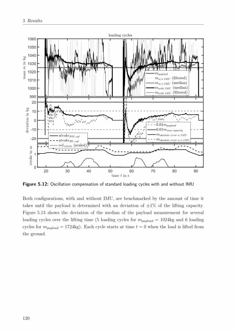
5 Results
990
1000
1010
1020
1030
1040
1050
1060
-20
-10
0
10
20
20 30 40 50 60 70 80 90
0
1
Figure 5.12: Oscillation compensation of standard loading cycles with and without IMU
Both configurations, with and without IMU, are benchmarked by the amount of time it
takes until the payload is determined with an deviation of ±1% of the lifting capacity.
Figure 5.13 shows the deviation of the median of the payload measurement for several
loading cycles over the lifting time (5 loading cycles for mpayload = 1024kg and 6 loading
cycles for mpayload = 1724kg). Each cycle starts at time t = 0 when the load is lifted from
the ground.
120
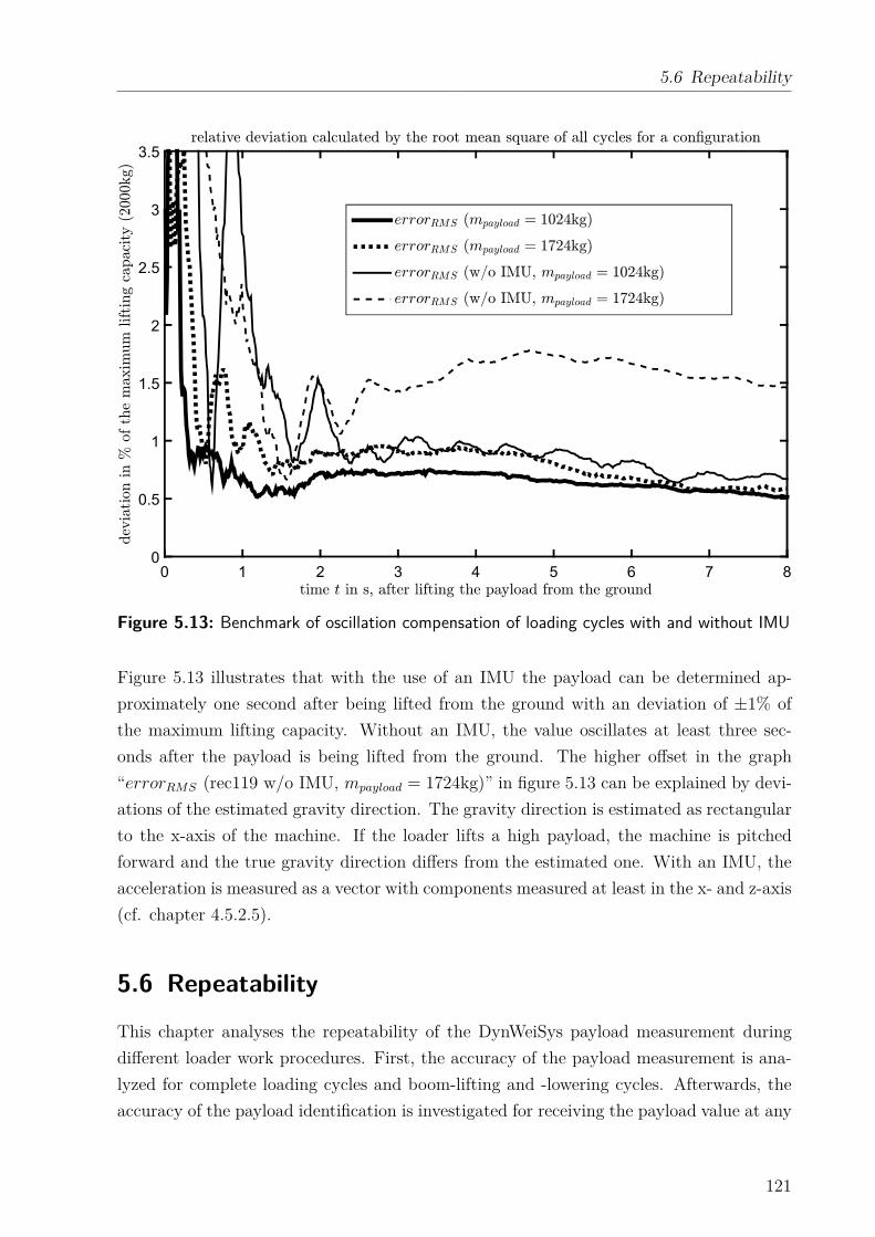
5.6 Repeatability
0 1 2 3 4 5 6 7 8
0
0.5
1
1.5
2
2.5
3
3.5
Figure 5.13: Benchmark of oscillation compensation of loading cycles with and without IMU
Figure 5.13 illustrates that with the use of an IMU the payload can be determined ap-
proximately one second after being lifted from the ground with an deviation of ±1% of
the maximum lifting capacity. Without an IMU, the value oscillates at least three sec-
onds after the payload is being lifted from the ground. The higher offset in the graph
“errorRMS (rec119 w/o IMU, mpayload = 1724kg)” in figure 5.13 can be explained by devi-
ations of the estimated gravity direction. The gravity direction is estimated as rectangular
to the x-axis of the machine. If the loader lifts a high payload, the machine is pitched
forward and the true gravity direction differs from the estimated one. With an IMU, the
acceleration is measured as a vector with components measured at least in the x- and z-axis
(cf. chapter 4.5.2.5).
5.6 Repeatability
This chapter analyses the repeatability of the DynWeiSys payload measurement during
different loader work procedures. First, the accuracy of the payload measurement is ana-
lyzed for complete loading cycles and boom-lifting and -lowering cycles. Afterwards, the
accuracy of the payload identification is investigated for receiving the payload value at any
121
5 Results
time during a continuous measurement.
Because the measurements do not follow a normal distribution, the following statistics
uses mainly medians and quartile ranges instead of mean values and standard deviations.
The results are shown in a box-whisker-plot. The bottom of the box exemplifies the first
quartile (25% quantile) whereas the top of the box represents the third quartile (75%
quantile). The line inside the box is the second quartile (50% quantile), also known as
the median. The whiskers have the length of 1.5 times of the inter quartile range (IQR),
which is 1.5 times the height of the box. This corresponds to approximately ±2.7σ and
the coverage of 99.3% if data is normally distributed. Data outside the whiskers is defined
as outliers. The width of the box is irrelevant, [Mat10].
5.6.1 Working Cycles
Several loading cycles are performed with a known payload that is permanently mounted
to the tool carrier of the front loader. At first, the payload is lifted from the ground and
fully supported by the front loader. While traveling forward, the load is fully raised, thus,
all cylinders are moved to match the desired working situation. Then, the bucket cylinders
are moved out simulating a dumping process onto a trailer. Finally, the bucket cylinders
are moved in back, the machine travels back, and the payload is lowered to the ground.
These cycles are performed several times with different known payloads while recording
the payload measurement. In addition, several lifting and lowering cycles of the boom are
included with different known weights to increase the number of measurements. To match
the desired working situation the boom and bucket actuators are moved. Afterwards, a
box-whisker-plot is generated and the median xi is calculated for each cycle, as displayed
in figures 5.14, A.18, A.19, A.20, A.21.
122
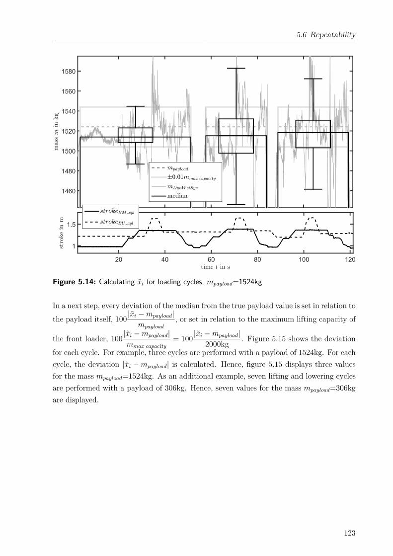
5.6 Repeatability
1460
1480
1500
1520
1540
1560
1580
20 40 60 80 100 120
1
1.5
Figure 5.14: Calculating xi for loading cycles, mpayload=1524kg
In a next step, every deviation of the median from the true payload value is set in relation to
the payload itself, 100|xi − mpayload|
mpayload
, or set in relation to the maximum lifting capacity of
the front loader, 100|xi − mpayload|mmax capacity
= 100|xi − mpayload|
2000kg. Figure 5.15 shows the deviation
for each cycle. For example, three cycles are performed with a payload of 1524kg. For each
cycle, the deviation |xi − mpayload| is calculated. Hence, figure 5.15 displays three values
for the mass mpayload=1524kg. As an additional example, seven lifting and lowering cycles
are performed with a payload of 306kg. Hence, seven values for the mass mpayload=306kg
are displayed.
123
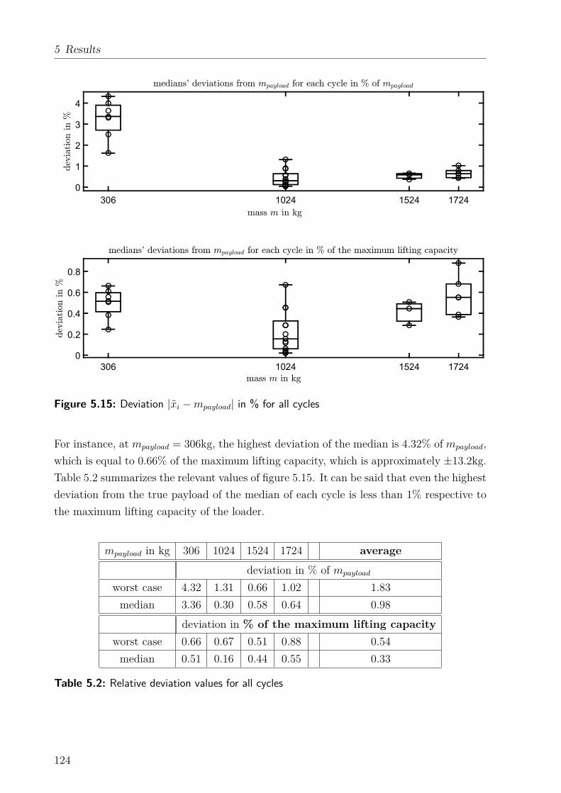
5 Results
306 1024 1524 1724
0
1
2
3
4
306 1024 1524 1724
0
0.2
0.4
0.6
0.8
Figure 5.15: Deviation |xi − mpayload| in % for all cycles
For instance, at mpayload = 306kg, the highest deviation of the median is 4.32% of mpayload,
which is equal to 0.66% of the maximum lifting capacity, which is approximately ±13.2kg.
Table 5.2 summarizes the relevant values of figure 5.15. It can be said that even the highest
deviation from the true payload of the median of each cycle is less than 1% respective to
the maximum lifting capacity of the loader.
mpayload in kg 306 1024 1524 1724 average
deviation in % of mpayload
worst case 4.32 1.31 0.66 1.02 1.83
median 3.36 0.30 0.58 0.64 0.98
deviation in % of the maximum lifting capacity
worst case 0.66 0.67 0.51 0.88 0.54
median 0.51 0.16 0.44 0.55 0.33
Table 5.2: Relative deviation values for all cycles
124
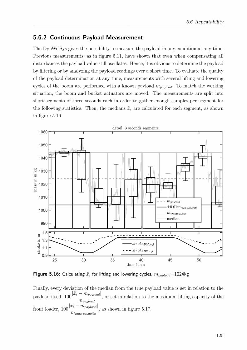
5.6 Repeatability
5.6.2 Continuous Payload Measurement
The DynWeiSys gives the possibility to measure the payload in any condition at any time.
Previous measurements, as in figure 5.11, have shown that even when compensating all
disturbances the payload value still oscillates. Hence, it is obvious to determine the payload
by filtering or by analyzing the payload readings over a short time. To evaluate the quality
of the payload determination at any time, measurements with several lifting and lowering
cycles of the boom are performed with a known payload mpayload. To match the working
situation, the boom and bucket actuators are moved. The measurements are split into
short segments of three seconds each in order to gather enough samples per segment for
the following statistics. Then, the medians xi are calculated for each segment, as shown
in figure 5.16.
990
1000
1010
1020
1030
1040
1050
1060
25 30 35 40 45 50
0.9
1.1
1.3
1.5
Figure 5.16: Calculating xi for lifting and lowering cycles, mpayload=1024kg
Finally, every deviation of the median from the true payload value is set in relation to the
payload itself, 100|xi − mpayload|
mpayload
, or set in relation to the maximum lifting capacity of the
front loader, 100|xi − mpayload|mmax capacity
, as shown in figure 5.17.
125
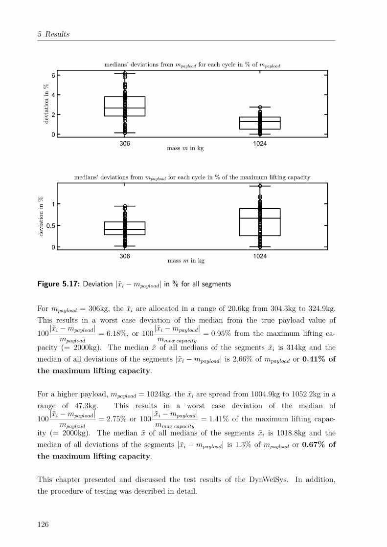
5 Results
306 1024
0
2
4
6
306 1024
0
0.5
1
Figure 5.17: Deviation |xi − mpayload| in % for all segments
For mpayload = 306kg, the xi are allocated in a range of 20.6kg from 304.3kg to 324.9kg.
This results in a worst case deviation of the median from the true payload value of
100|xi − mpayload|
mpayload
= 6.18%, or 100|xi − mpayload|mmax capacity
= 0.95% from the maximum lifting ca-
pacity (= 2000kg). The median x of all medians of the segments xi is 314kg and the
median of all deviations of the segments |xi − mpayload| is 2.66% of mpayload or 0.41% of
the maximum lifting capacity.
For a higher payload, mpayload = 1024kg, the xi are spread from 1004.9kg to 1052.2kg in a
range of 47.3kg. This results in a worst case deviation of the median of
100|xi − mpayload|
mpayload
= 2.75% or 100|xi − mpayload|mmax capacity
= 1.41% of the maximum lifting capac-
ity (= 2000kg). The median x of all medians of the segments xi is 1018.8kg and the
median of all deviations of the segments |xi − mpayload| is 1.3% of mpayload or 0.67% of
the maximum lifting capacity.
This chapter presented and discussed the test results of the DynWeiSys. In addition,
the procedure of testing was described in detail.
126
6 Conclusion and Outlook
This thesis deals with the research and development of a mobile loader scale, “Dynamic
Weighing System” (DynWeiSys), which measures a lifted payload in every working situa-
tion. A prototype is developed for a front loader of an agricultural tractor that measures
payload continuously with a deviation of ±1% of the maximum payload capacity regardless
of the center of gravity position of the payload or whether the machine moves, travels, or
bounces. The underlying theory combines a static model with a multi-body model.
The static model considers all front loader dimensions and transfers the measured ac-
tuator forces with the knowledge of the loader kinematics into torques at the joints of an
open, planar kinematic chain. The chain consists of three major parts: chassis, boom,
and tool carrier with two joints in between. The multi-body model is used to transfer
measured accelerations into forces. The forces in connection with their respective levers
generate torques at the joints as well. These torques are set into relation to each other.
Since the multi-body model considers a front loader without a payload, the torques from
the static model and the torques from the multi-body model differ from each other, which
allows to calculate the payload.
The payload measurement is independent of the center of gravity position of the payload.
This is achieved by considering the torques at both joints of the open planar kinematic
chain, which implies the use of both boom and bucket actuator forces. Hence, the payload
measurement is possible with any attached tool without an additional calibration. It is
irrelevant whether the center of gravity of the payload is close to the machine, as for a
bucket, or further away, for instance, in case of a bale clamp. This even applies to a tool
with an additional moving arm such as a crane or excavator attachment.
Due to the cylinder and joint friction, the measured actuator forces deviate from the real
actuator forces. Hence, friction is estimated with a friction model and is considered in the
payload measurement. While working with the front loader, the measured actuator forces
contain oscillations which are caused by the movements of the front loader and disturb
the payload measurement. To compensate the influence of the movements on the payload
measurement, the multi-body model is provided with accelerations that are measured with
an inertial measurement unit (IMU). If the accelerations are not measured but considered
as constant (gravity acceleration), the oscillations are directly transferred to the payload
signal. Nevertheless, it is possible to determine the payload, but it takes more time due to
filtering of the signal. If the acceleration is considered as constant (gravity), the direction
127
6 Conclusion and Outlook
of the gravity is generally assumed as rectangular to the x-axis of the machine. A tilted
machine, for instance while working on a slope, causes errors in the payload measurement
because the direction of the gravity is still assumed as rectangular to the x-axis of the
machine. These errors can be compensated with an additional tilt sensor. However, mea-
suring the acceleration with an IMU compensates tilting of the machine anyway because
the direction of the acceleration is measured as vector.
Although influences of the movements of the front loader are almost compensated, the
payload signal still yields noises and oscillations, which are caused by sensor noises and
time lags between the sensor signals. These effects are reduced by filtering the calculated
payload signal with a low-pass filter to obtain a suitable signal.
The accuracy of the payload measurement strongly relies on the accuracy of the mod-
els. Developing an accurate multi-body model and identifying all its parameters is very
time-consuming. Either the model and its parameters are derived from 3D-CAD data or
a real front loader is taken apart and each parameter is measured in tests as done in this
thesis. A model derived from 3D-CAD data underlies manufacturing tolerances and does
not consider changes that are made on the front loader afterwards, such as adding an
additional valve to the boom. Deriving the parameters of the multi-body model by tests,
takes a lot of effort, but it is very accurate for one loader. Nevertheless, it has to be done
for every machine.
This led to the development of a reduced multi-body model that obtains its parame-
ters partly from 3D-CAD data and partly from a short calibration procedure. Thus, the
reduced multi-body model is self-adjusting and covers all manufacturing tolerances. To
consider changes that are made on the front loader afterwards, the calibration procedure
can easily be redone.
To measure payload continuously at any time, the static model and the multi-body model
require a continuous position detection of the front loader relative to the tractor. To obtain
a reliable measurement system which is also easy to retrofit on existing loaders, the posi-
tion detection is implemented with three IMUs connected to the chassis, boom, and tool
carrier. The IMUs only consist of non-moving parts and can be mounted anywhere in a
protected position. The accuracy of the position detection of the front loader and also the
accuracy of the payload measurement is highly dependent on the accuracy of the IMUs.
Tests showed that the acceleration measurements of the IMUs for different axis strongly
deviate from the real acceleration due to tolerances. For instance, the signal deviates ap-
proximately 4% from the gravity during standstill. In this case, an additional calibration
128
is required to correct the output of the IMUs.
The payload should be determined as quickly as possible. Considering an average loading
cycle which lasts 10 to 20 seconds only a fraction of that time allows to determine the
payload. The remaining time is spent on picking up the load, dumping, and returning to
the pick up place. If the signal processing contains a logic that counts loading cycles and
determines payload of each cycle automatically, an instant payload signal is required. Fi-
nally, the DynWeiSys developed in this thesis generates a continuous payload signal which
allows further analysis. The signal determines the weight of the payload as quickly as
possible. Figure 5.13 in chapter 5.5 shows that it takes about one second after lifting the
payload from the ground to determine the weight of the payload with an accuracy loss of
±1% of the maximum lifting capacity.
The DynWeiSys, as developed in this thesis, provides a continuous weight signal of the
payload in every working situation after being lifted from the ground. To increase the
benefit of the DynWeiSys, a “Weighing Logic” can be implemented that identifies load-
ing cycles such as payload pick up, dumping, removing, or adding. The “Weighing Logic”
counts the cycles and accumulates or subtracts the payload automatically and gives a com-
prehensive analysis of the handled material to the operator. This data allows the operator
to evaluate or to bill the handled material immediately. Transferring this data continu-
ously to a data processing server allows the mobile scale to be integrated and linked to the
work environment, such as logistic, pricing, or payment systems. Also, service cycles of the
front loader can be matched to the amount of the handled payload because a constantly
used machine needs more service than a machine that is idle most of the time. Also, wear
at the actuators or joints can be detected by deviations of the internal friction calculation.
In the following, several issues for further research are proposed to optimize the Dyn-
WeiSys as it is described in this thesis. In this regard, the friction model could be im-
proved. During the movements of the front loader, the friction has a huge influence on
the measurement accuracy. In this thesis, a pressure based friction model is applied with
a friction behavior that is linearly proportional to the cylinder pressures. The parameters
of this friction model are determined by measurements performed directly at the front
loader itself. It is recommended to continue research by examining the friction behavior
of hydraulic cylinders on a test bench and use the results to enhance the current friction
model.
Currently, the DynWeiSys considers measured accelerations to calculate the payload. At
standstill, these accelerations must be the gravity. Hence, it is suggested to detect stand-
129
6 Conclusion and Outlook
still and calibrate the output of the IMUs to minimize tolerances. Additionally, switching
between measured accelerations and a constant gravity serves as a possibility to avoid
sensor noise.
To calculate the actuator forces, the pressures are taken at the hydraulic line just next
to the cylinders. To minimize the influence of pressure drop due to oil flow, it is recom-
mended to change the design of the cylinders to include pressure sensors that measure the
pressures directly in the cylinder. This also decreases the influence of the oil viscosities
due to changing temperatures.
A common working procedure is to operate the cylinders at the end-stroke positions. For
instance, the bucket cylinders are frequently driven at the minimum end-stroke position,
also known as the rollback position. If the hydraulic actuators are in the end-stroke po-
sitions, a determination of the actuator forces by hydraulic pressures is not possible. It
is suggested to search for a solution either to avoid these positions or to provide actuator
forces in these positions.
Heavy payloads cause elastic deformations on the structure of the front loader. This
will change the dimensions, for instance, the distance between the main joints, chassis,
boom, and tool carrier will decrease. It is suggested to continue research by compensating
the elastic deformations of the structure by adjusting the dimensions of the static model
in relation to the payload.
In this thesis, the DynWeiSys is shown as an example applied on a non self-leveling agri-
cultural front loader. The next steps could be the transfer of the system to different loader
kinematics such as mechanical self leveling loader kinematics or wheel loader kinematics.
130
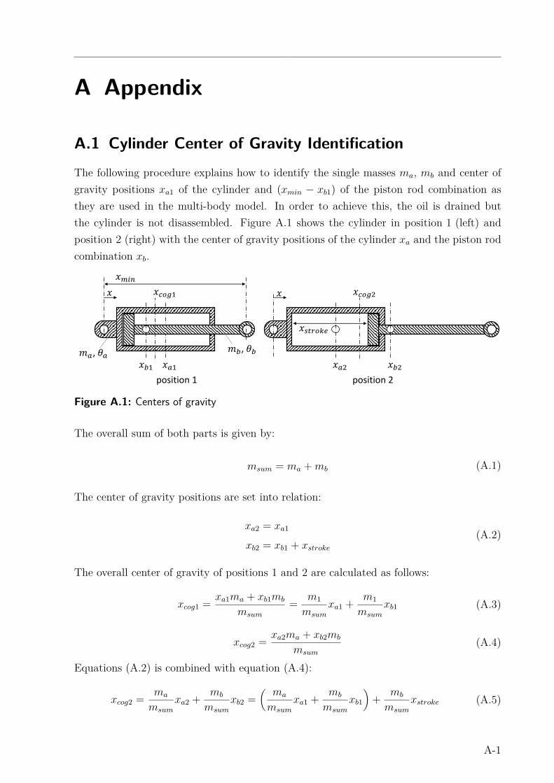
A Appendix
A.1 Cylinder Center of Gravity Identification
The following procedure explains how to identify the single masses ma, mb and center of
gravity positions xa1 of the cylinder and (xmin − xb1) of the piston rod combination as
they are used in the multi-body model. In order to achieve this, the oil is drained but
the cylinder is not disassembled. Figure A.1 shows the cylinder in position 1 (left) and
position 2 (right) with the center of gravity positions of the cylinder xa and the piston rod
combination xb.
, � , �� �
�� � �� ��
� � � �� �
position 1 position 2
Figure A.1: Centers of gravity
The overall sum of both parts is given by:
msum = ma + mb (A.1)
The center of gravity positions are set into relation:
xa2 = xa1
xb2 = xb1 + xstroke
(A.2)
The overall center of gravity of positions 1 and 2 are calculated as follows:
xcog1 =xa1ma + xb1mb
msum
=m1
msum
xa1 +m1
msum
xb1 (A.3)
xcog2 =xa2ma + xb2mb
msum(A.4)
Equations (A.2) is combined with equation (A.4):
xcog2 =ma
msum
xa2 +mb
msum
xb2 =(
ma
msum
xa1 +mb
msum
xb1
)
+mb
msum
xstroke (A.5)
A-1
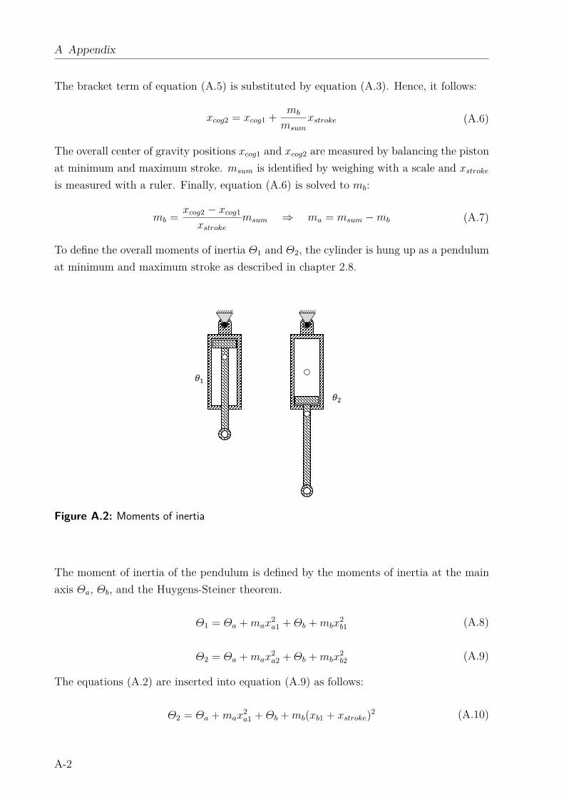
A Appendix
The bracket term of equation (A.5) is substituted by equation (A.3). Hence, it follows:
xcog2 = xcog1 +mb
msum
xstroke (A.6)
The overall center of gravity positions xcog1 and xcog2 are measured by balancing the piston
at minimum and maximum stroke. msum is identified by weighing with a scale and xstroke
is measured with a ruler. Finally, equation (A.6) is solved to mb:
mb =xcog2 − xcog1
xstroke
msum ⇒ ma = msum − mb (A.7)
To define the overall moments of inertia Θ1 and Θ2, the cylinder is hung up as a pendulum
at minimum and maximum stroke as described in chapter 2.8.
��
Figure A.2: Moments of inertia
The moment of inertia of the pendulum is defined by the moments of inertia at the main
axis Θa, Θb, and the Huygens-Steiner theorem.
Θ1 = Θa + max2a1 + Θb + mbx
2b1 (A.8)
Θ2 = Θa + max2a2 + Θb + mbx
2b2 (A.9)
The equations (A.2) are inserted into equation (A.9) as follows:
Θ2 = Θa + max2a1 + Θb + mb(xb1 + xstroke)
2 (A.10)
A-2
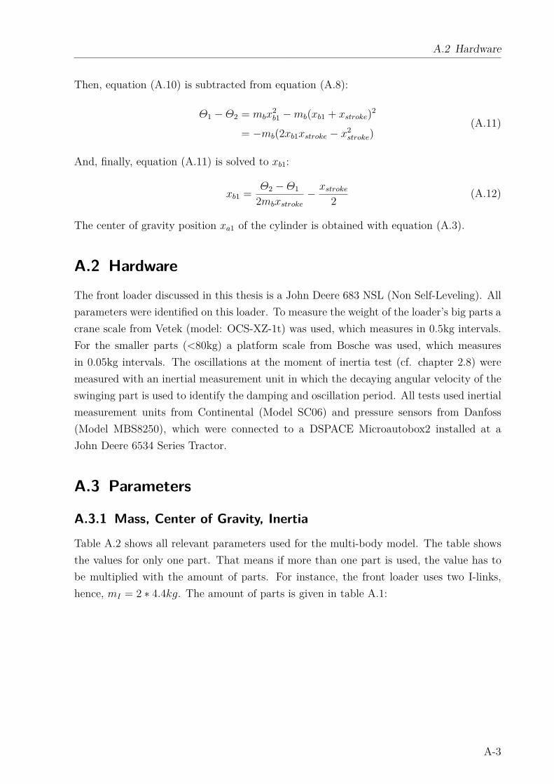
A.2 Hardware
Then, equation (A.10) is subtracted from equation (A.8):
Θ1 − Θ2 = mbx2b1 − mb(xb1 + xstroke)
2
= −mb(2xb1xstroke − x2stroke)
(A.11)
And, finally, equation (A.11) is solved to xb1:
xb1 =Θ2 − Θ1
2mbxstroke
− xstroke
2(A.12)
The center of gravity position xa1 of the cylinder is obtained with equation (A.3).
A.2 Hardware
The front loader discussed in this thesis is a John Deere 683 NSL (Non Self-Leveling). All
parameters were identified on this loader. To measure the weight of the loader’s big parts a
crane scale from Vetek (model: OCS-XZ-1t) was used, which measures in 0.5kg intervals.
For the smaller parts (<80kg) a platform scale from Bosche was used, which measures
in 0.05kg intervals. The oscillations at the moment of inertia test (cf. chapter 2.8) were
measured with an inertial measurement unit in which the decaying angular velocity of the
swinging part is used to identify the damping and oscillation period. All tests used inertial
measurement units from Continental (Model SC06) and pressure sensors from Danfoss
(Model MBS8250), which were connected to a DSPACE Microautobox2 installed at a
John Deere 6534 Series Tractor.
A.3 Parameters
A.3.1 Mass, Center of Gravity, Inertia
Table A.2 shows all relevant parameters used for the multi-body model. The table shows
the values for only one part. That means if more than one part is used, the value has to
be multiplied with the amount of parts. For instance, the front loader uses two I-links,
hence, mI = 2 ∗ 4.4kg. The amount of parts is given in table A.1:
A-3
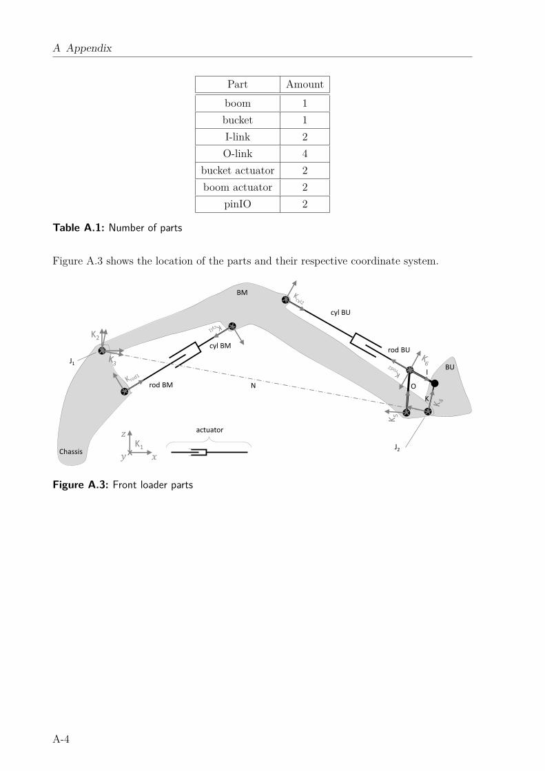
A Appendix
Part Amount
boom 1
bucket 1
I-link 2
O-link 4
bucket actuator 2
boom actuator 2
pinIO 2
Table A.1: Number of parts
Figure A.3 shows the location of the parts and their respective coordinate system.
J1
J2
BM
BU
K
O
I
cyl BM
cyl BU
rod BU
rod BM
Chassis
N
actuator
K2
K1 ��Figure A.3: Front loader parts
A-4
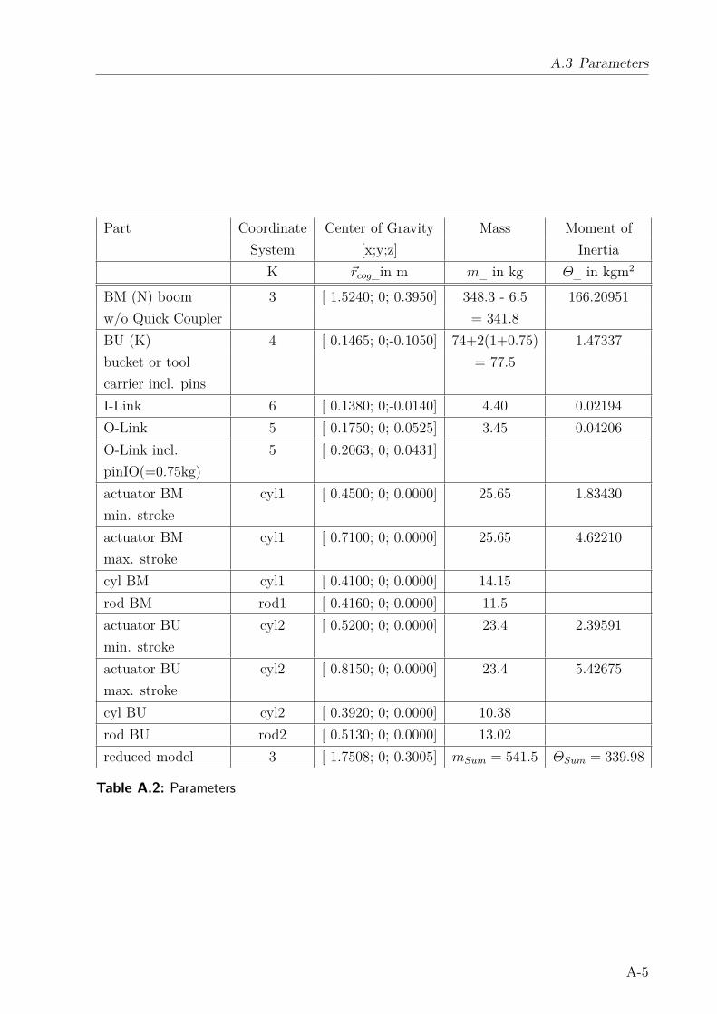
A.3 Parameters
Part Coordinate Center of Gravity Mass Moment of
System [x;y;z] Inertia
K ~rcog_in m m_ in kg Θ_ in kgm2
BM (N) boom 3 [ 1.5240; 0; 0.3950] 348.3 - 6.5 166.20951
w/o Quick Coupler = 341.8
BU (K) 4 [ 0.1465; 0;-0.1050] 74+2(1+0.75) 1.47337
bucket or tool
carrier incl. pins
= 77.5
I-Link 6 [ 0.1380; 0;-0.0140] 4.40 0.02194
O-Link 5 [ 0.1750; 0; 0.0525] 3.45 0.04206
O-Link incl.
pinIO(=0.75kg)
5 [ 0.2063; 0; 0.0431]
actuator BM
min. stroke
cyl1 [ 0.4500; 0; 0.0000] 25.65 1.83430
actuator BM
max. stroke
cyl1 [ 0.7100; 0; 0.0000] 25.65 4.62210
cyl BM cyl1 [ 0.4100; 0; 0.0000] 14.15
rod BM rod1 [ 0.4160; 0; 0.0000] 11.5
actuator BU
min. stroke
cyl2 [ 0.5200; 0; 0.0000] 23.4 2.39591
actuator BU
max. stroke
cyl2 [ 0.8150; 0; 0.0000] 23.4 5.42675
cyl BU cyl2 [ 0.3920; 0; 0.0000] 10.38
rod BU rod2 [ 0.5130; 0; 0.0000] 13.02
reduced model 3 [ 1.7508; 0; 0.3005] mSum = 541.5 ΘSum = 339.98
Table A.2: Parameters
A-5
A Appendix
In the following list, several notes are given related to the parameters of table A.2:
• Each moment of inertia is given for the main axis in y-direction.
• The parameters for the reduced model are calculated by:
mSum = mBM +mBU +2mI +4mO+2mpinIO+2mBMcyl+2mBMrod+2mBUcyl+2mBUrod
To estimate the moment of inertia, the loader is assumed as a square box with the
length of the boom and a height of 0.3m. This results in the following equation:
ΘSum = (mSum − mBU)(N2 + 0.32)/12 = (mSum − mBU)(2.952 + 0.32)/12). (A.13)
• Pins of the loader joints must be considered. In order to not consider a pin twice, it
has to be determined to which part it belongs.
• A hydraulic cylinder that has different oil capacities at different strokes is considered
as two parts, namely as cylinder and piston with rod. A procedure to identify
the centers of gravity for rod and cylinder without disassembling the actuator, is
discussed in section A.1. The mass of the oil volume in the cylinder is not considered.
A-6
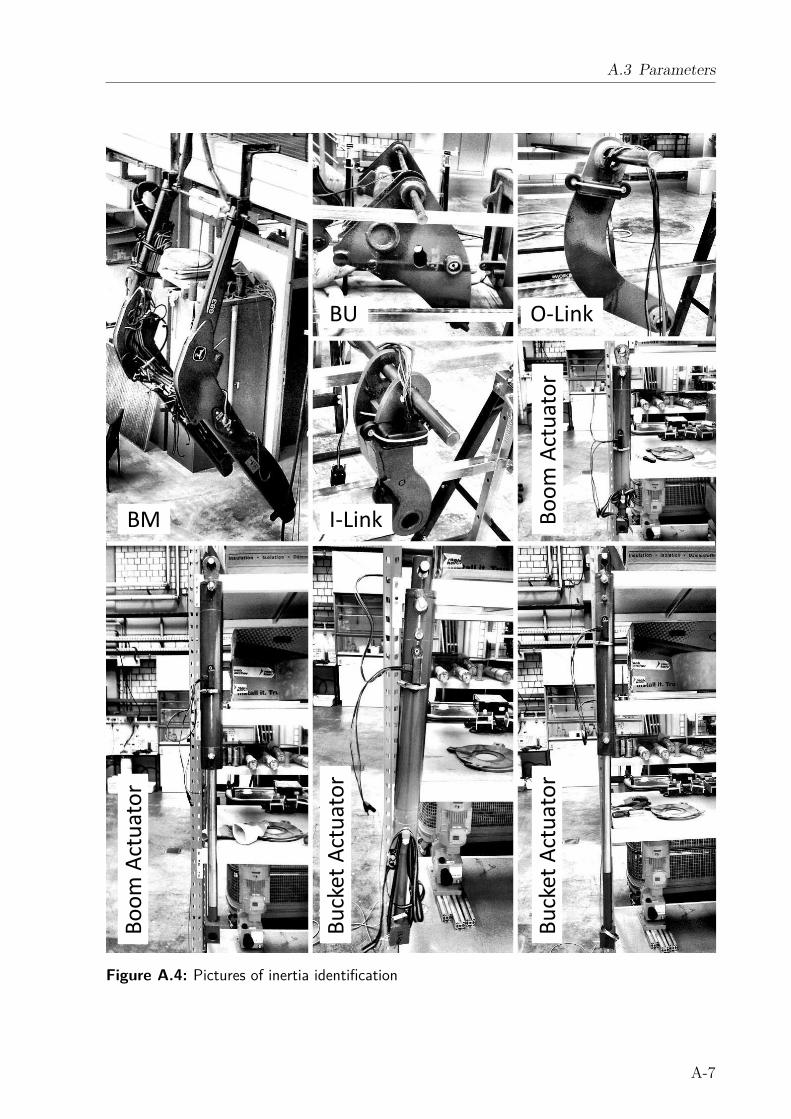
A.3 Parameters
BM I-Link
O-LinkBU
Bo
om
Act
ua
tor
Bo
om
Act
ua
tor
Bu
cke
t A
ctu
ato
r
Bu
cke
t A
ctu
ato
r
Figure A.4: Pictures of inertia identification
A-7
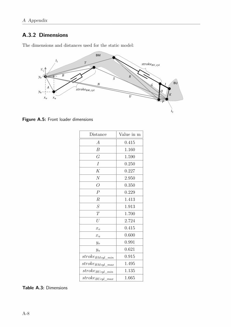
A Appendix
A.3.2 Dimensions
The dimensions and distances used for the static model:
J1
J2
� ���_�
BM
BU
��� ���_�� �
�K2
Figure A.5: Front loader dimensions
Distance Value in m
A 0.415
B 1.160
G 1.590
I 0.250
K 0.227
N 2.950
O 0.350
P 0.229
R 1.413
S 1.913
T 1.700
U 2.724
xo 0.415
xu 0.600
yo 0.991
yu 0.621
strokeBMcyl_min 0.915
strokeBMcyl_max 1.495
strokeBUcyl_min 1.135
strokeBUcyl_max 1.665
Table A.3: Dimensions
A-8
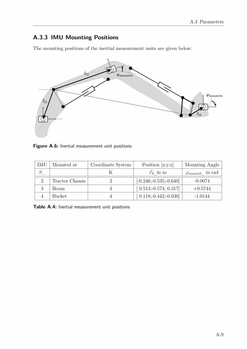
A.3 Parameters
A.3.3 IMU Mounting Positions
The mounting positions of the inertial measurement units are given below:
2 �
�
�
� �� �
Figure A.6: Inertial measurement unit positions
IMU Mounted at Coordinate System Position [x;y;z] Mounting Angle
S_ K ~rS_in m ϕmountS_ in rad
2 Tractor Chassis 2 [-0.246;-0.535;-0.640] -0.0074
3 Boom 3 [ 0.513;-0.574; 0.317] +0.5744
4 Bucket 4 [ 0.118;-0.442;-0.030] -1.0144
Table A.4: Inertial measurement unit positions
A-9
A Appendix
A.3.4 Cylinder Dimensions
Dimensions of the boom and bucket cylinders of the front loader used in this thesis:
Position Part Variable Diameter
D in m
Boom Piston DBMpiston 0.08
Boom Piston Dseal_innerDiameter 0.06
Boom Rod DBMrod 0.04
Boom Rod Dseal_outerDiameter 0.05
Bucket Piston DBUpiston 0.07
Bucket Piston Dseal_innerDiameter 0.06
Bucket Rod DBUrod 0.04
Bucket Rod Dseal_outerDiameter 0.05
Table A.5: Actuator diameters
Notice, that two cylinders are used per function, two bucket cylinders and two boom
cylinders.
A.4 Fluid Film Thickness
The assumptions to calculate the thickness of the lubrication film are as follows: the
hydrodynamic pressure between seal and surface is in balance with the local seal load
which is given by the mounting pre-load, its shape, and the hydraulic pressure within the
cylinder. A detailed explanation of this is given in chapter 5 of reference [MN13].
A-10
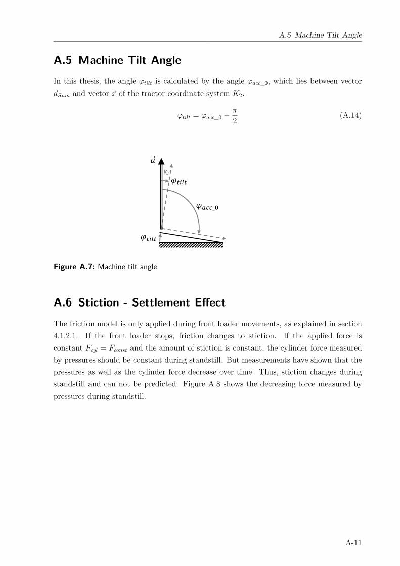
A.5 Machine Tilt Angle
A.5 Machine Tilt Angle
In this thesis, the angle ϕtilt is calculated by the angle ϕacc_0, which lies between vector
~aSum and vector ~x of the tractor coordinate system K2.
ϕtilt = ϕacc_0 − π
2(A.14)
� _0
�
� �
� �
Figure A.7: Machine tilt angle
A.6 Stiction - Settlement Effect
The friction model is only applied during front loader movements, as explained in section
4.1.2.1. If the front loader stops, friction changes to stiction. If the applied force is
constant Fcyl = Fconst and the amount of stiction is constant, the cylinder force measured
by pressures should be constant during standstill. But measurements have shown that the
pressures as well as the cylinder force decrease over time. Thus, stiction changes during
standstill and can not be predicted. Figure A.8 shows the decreasing force measured by
pressures during standstill.
A-11
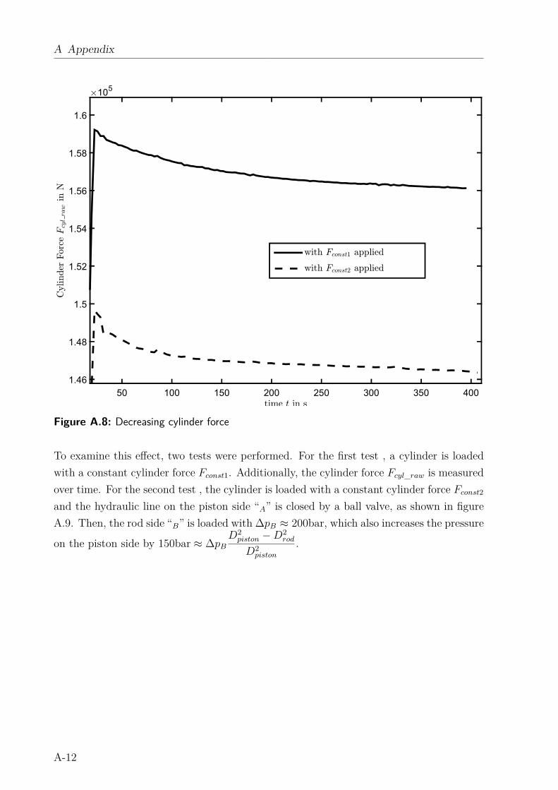
A Appendix
50 100 150 200 250 300 350 400
105
1.46
1.48
1.5
1.52
1.54
1.56
1.58
1.6
Figure A.8: Decreasing cylinder force
To examine this effect, two tests were performed. For the first test , a cylinder is loaded
with a constant cylinder force Fconst1. Additionally, the cylinder force Fcyl_raw is measured
over time. For the second test , the cylinder is loaded with a constant cylinder force Fconst2
and the hydraulic line on the piston side “A” is closed by a ball valve, as shown in figure
A.9. Then, the rod side “B” is loaded with ∆pB ≈ 200bar, which also increases the pressure
on the piston side by 150bar ≈ ∆pB
D2piston − D2
rod
D2piston
.
A-12
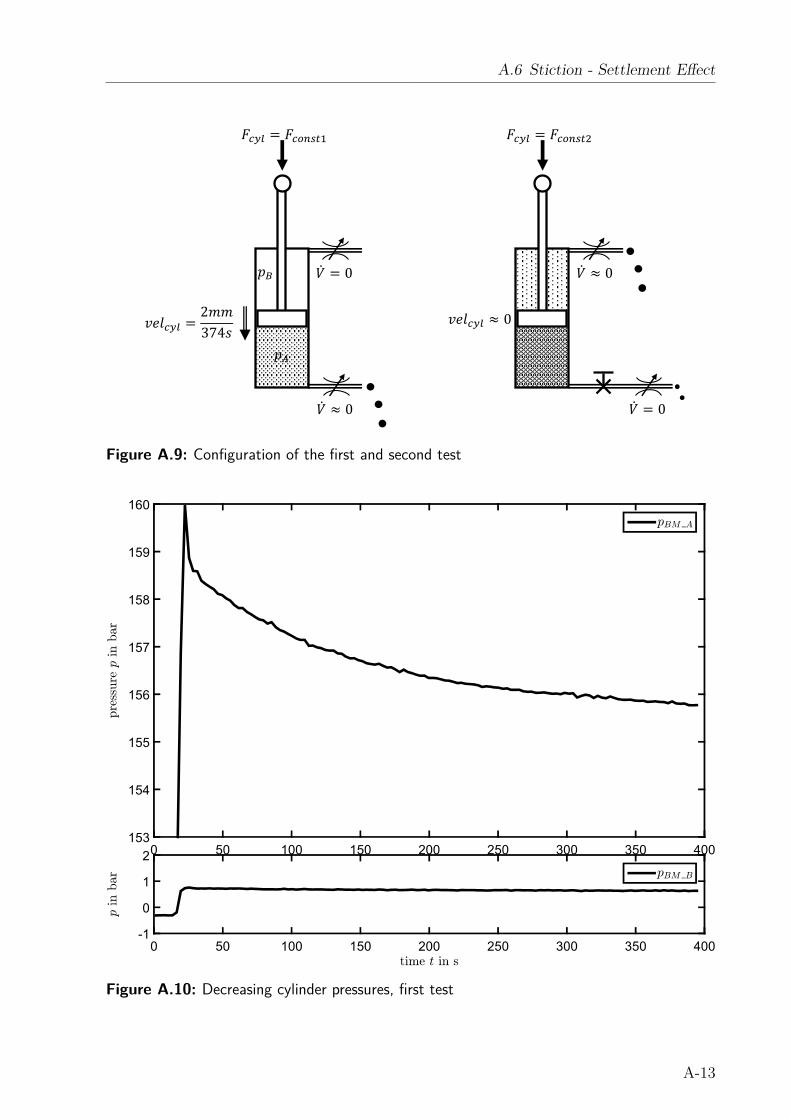
A.6 Stiction - Settlement Effect
� = � �
�� = 274�
� �� ��
�� ≈ 0 � ≈ 0
� = 0 � ≈ 0
� = 0
� = � �
Figure A.9: Configuration of the first and second test
0 50 100 150 200 250 300 350 400
153
154
155
156
157
158
159
160
0 50 100 150 200 250 300 350 400
-1
0
1
2
Figure A.10: Decreasing cylinder pressures, first test
A-13
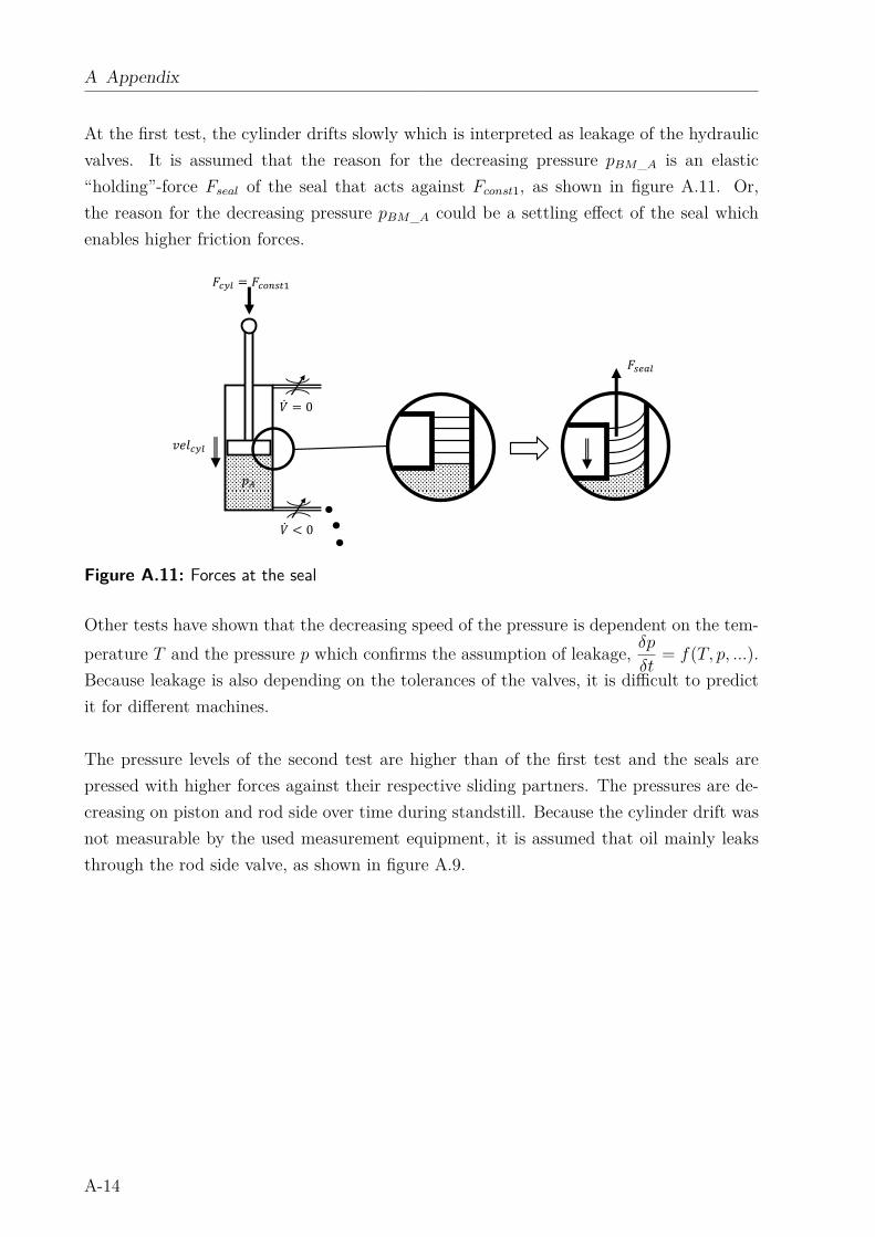
A Appendix
At the first test, the cylinder drifts slowly which is interpreted as leakage of the hydraulic
valves. It is assumed that the reason for the decreasing pressure pBM_A is an elastic
“holding”-force Fseal of the seal that acts against Fconst1, as shown in figure A.11. Or,
the reason for the decreasing pressure pBM_A could be a settling effect of the seal which
enables higher friction forces.
� = � �
�� � < 0
� = 0�
Figure A.11: Forces at the seal
Other tests have shown that the decreasing speed of the pressure is dependent on the tem-
perature T and the pressure p which confirms the assumption of leakage,δp
δt= f(T, p, ...).
Because leakage is also depending on the tolerances of the valves, it is difficult to predict
it for different machines.
The pressure levels of the second test are higher than of the first test and the seals are
pressed with higher forces against their respective sliding partners. The pressures are de-
creasing on piston and rod side over time during standstill. Because the cylinder drift was
not measurable by the used measurement equipment, it is assumed that oil mainly leaks
through the rod side valve, as shown in figure A.9.
A-14
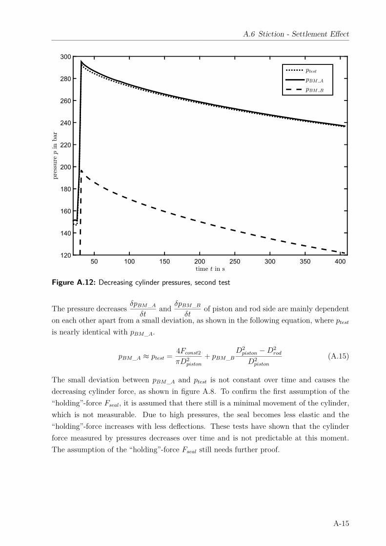
A.6 Stiction - Settlement Effect
50 100 150 200 250 300 350 400
120
140
160
180
200
220
240
260
280
300
Figure A.12: Decreasing cylinder pressures, second test
The pressure decreasesδpBM_A
δtand
δpBM_B
δtof piston and rod side are mainly dependent
on each other apart from a small deviation, as shown in the following equation, where ptest
is nearly identical with pBM_A.
pBM_A ≈ ptest =4Fconst2
πD2piston
+ pBM_B
D2piston − D2
rod
D2piston
(A.15)
The small deviation between pBM_A and ptest is not constant over time and causes the
decreasing cylinder force, as shown in figure A.8. To confirm the first assumption of the
“holding”-force Fseal, it is assumed that there still is a minimal movement of the cylinder,
which is not measurable. Due to high pressures, the seal becomes less elastic and the
“holding”-force increases with less deflections. These tests have shown that the cylinder
force measured by pressures decreases over time and is not predictable at this moment.
The assumption of the “holding”-force Fseal still needs further proof.
A-15
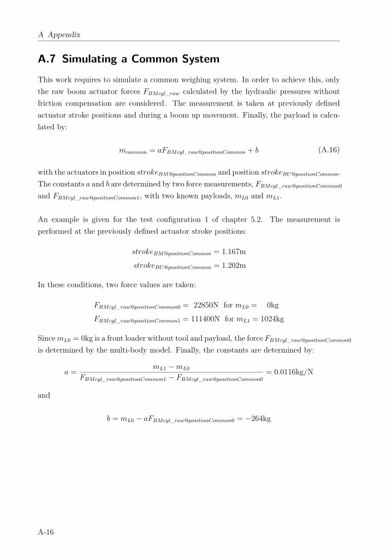
A Appendix
A.7 Simulating a Common System
This work requires to simulate a common weighing system. In order to achieve this, only
the raw boom actuator forces FBMcyl_raw calculated by the hydraulic pressures without
friction compensation are considered. The measurement is taken at previously defined
actuator stroke positions and during a boom up movement. Finally, the payload is calcu-
lated by:
mcommon = aFBMcyl_raw@positionCommon + b (A.16)
with the actuators in position strokeBM@positionCommon and position strokeBU@positionCommon.
The constants a and b are determined by two force measurements, FBMcyl_raw@positionCommon0
and FBMcyl_raw@positionCommon1, with two known payloads, mL0 and mL1.
An example is given for the test configuration 1 of chapter 5.2. The measurement is
performed at the previously defined actuator stroke positions:
strokeBM@positionCommon = 1.167m
strokeBU@positionCommon = 1.202m
In these conditions, two force values are taken:
FBMcyl_raw@positionCommon0 = 22850N for mL0 = 0kg
FBMcyl_raw@positionCommon1 = 111400N for mL1 = 1024kg
Since mL0 = 0kg is a front loader without tool and payload, the force FBMcyl_raw@positionCommon0
is determined by the multi-body model. Finally, the constants are determined by:
a =mL1 − mL0
FBMcyl_raw@positionCommon1 − FBMcyl_raw@positionCommon0
= 0.0116kg/N
and
b = mL0 − aFBMcyl_raw@positionCommon0 = −264kg
A-16
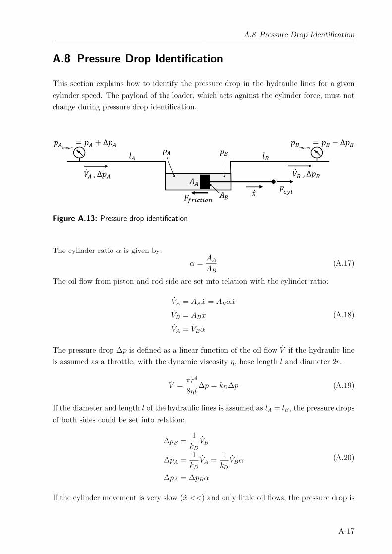
A.8 Pressure Drop Identification
A.8 Pressure Drop Identification
This section explains how to identify the pressure drop in the hydraulic lines for a given
cylinder speed. The payload of the loader, which acts against the cylinder force, must not
change during pressure drop identification.
= + ∆ �
� � , ∆ �� �� �� �� , ∆ �� = � − ∆ �
� ���
Figure A.13: Pressure drop identification
The cylinder ratio α is given by:
α =AA
AB
(A.17)
The oil flow from piston and rod side are set into relation with the cylinder ratio:
VA = AAx = ABαx
VB = ABx
VA = VBα
(A.18)
The pressure drop ∆p is defined as a linear function of the oil flow V if the hydraulic line
is assumed as a throttle, with the dynamic viscosity η, hose length l and diameter 2r.
V =πr4
8ηl∆p = kD∆p (A.19)
If the diameter and length l of the hydraulic lines is assumed as lA = lB, the pressure drops
of both sides could be set into relation:
∆pB =1
kD
VB
∆pA =1
kD
VA =1
kD
VBα
∆pA = ∆pBα
(A.20)
If the cylinder movement is very slow (x <<) and only little oil flows, the pressure drop is
A-17
A Appendix
negligibly small, ∆pA ≈ ∆pB ≈ 0
pAmeas1≈ pA
pBmeas1≈ pB
(A.21)
At a fast cylinder movement (x >) the pressure drop disturbs the measurement,
∆pA 6= 0 and ∆pB 6= 0. The pressures at the sensor positions are defined as follows:
pAmeas2= pA + ∆pA → pA = pAmeas2
− ∆pA
pBmeas2= pA − ∆pB → pB = pBmeas2
+ ∆pB
(A.22)
The force balance at the cylinder is given by:
Fcyl
AB
= pAα − pB − Ffriction
AB
(A.23)
The force balances of the slow and fast movement are set into relation:
Fcyl
AB
= pAmeas1α − pBmeas1
− Ffriction
AB
= (pAmeas2− ∆pA)α − (pBmeas2
+ ∆pB) − Ffriction
AB
(A.24)
Due to the unchanged payload, the friction is assumed as equal for the slow and fast lifting
cycle and is eliminated.
pAmeas1α − pBmeas1
= pAmeas2α − pBmeas2
− (∆pAα + ∆pB)
α(pAmeas1− pAmeas2
) − (pBmeas1− pBmeas2
) = −(∆pAα + ∆pB)(A.25)
Finally, the equation (A.25) is solved to ∆pB with ∆pA = ∆pBα:
α(pAmeas2− pAmeas1
) − (pBmeas2− pBmeas1
)
α2 + 1= ∆pB (A.26)
Note: Mobile scale manufacturers often generate different cylinder speeds for the calibra-
tion with different engine speeds and the joystick at full stroke.
A-18
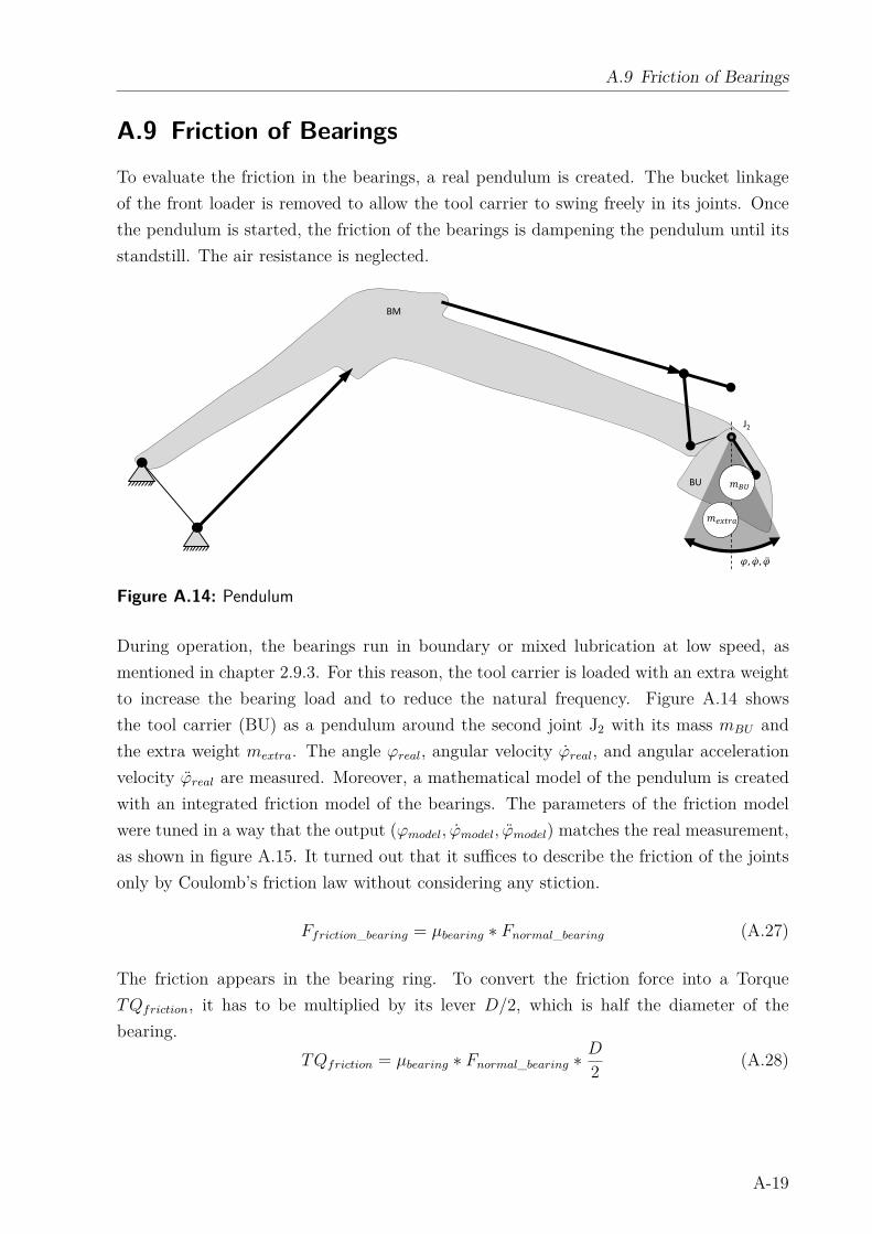
A.9 Friction of Bearings
A.9 Friction of Bearings
To evaluate the friction in the bearings, a real pendulum is created. The bucket linkage
of the front loader is removed to allow the tool carrier to swing freely in its joints. Once
the pendulum is started, the friction of the bearings is dampening the pendulum until its
standstill. The air resistance is neglected.
BM
BU ���
J2
�, �, �Figure A.14: Pendulum
During operation, the bearings run in boundary or mixed lubrication at low speed, as
mentioned in chapter 2.9.3. For this reason, the tool carrier is loaded with an extra weight
to increase the bearing load and to reduce the natural frequency. Figure A.14 shows
the tool carrier (BU) as a pendulum around the second joint J2 with its mass mBU and
the extra weight mextra. The angle ϕreal, angular velocity ϕreal, and angular acceleration
velocity ϕreal are measured. Moreover, a mathematical model of the pendulum is created
with an integrated friction model of the bearings. The parameters of the friction model
were tuned in a way that the output (ϕmodel, ϕmodel, ϕmodel) matches the real measurement,
as shown in figure A.15. It turned out that it suffices to describe the friction of the joints
only by Coulomb’s friction law without considering any stiction.
Ffriction_bearing = µbearing ∗ Fnormal_bearing (A.27)
The friction appears in the bearing ring. To convert the friction force into a Torque
TQfriction, it has to be multiplied by its lever D/2, which is half the diameter of the
bearing.
TQfriction = µbearing ∗ Fnormal_bearing ∗ D
2(A.28)
A-19
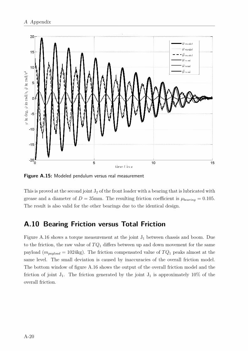
A Appendix
Figure A.15: Modeled pendulum versus real measurement
This is proved at the second joint J2 of the front loader with a bearing that is lubricated with
grease and a diameter of D = 35mm. The resulting friction coefficient is µbearing = 0.105.
The result is also valid for the other bearings due to the identical design.
A.10 Bearing Friction versus Total Friction
Figure A.16 shows a torque measurement at the joint J1 between chassis and boom. Due
to the friction, the raw value of TQ1 differs between up and down movement for the same
payload (mpayload = 1024kg). The friction compensated value of TQ1 peaks almost at the
same level. The small deviation is caused by inaccuracies of the overall friction model.
The bottom window of figure A.16 shows the output of the overall friction model and the
friction of joint J1. The friction generated by the joint J1 is approximately 10% of the
overall friction.
A-20
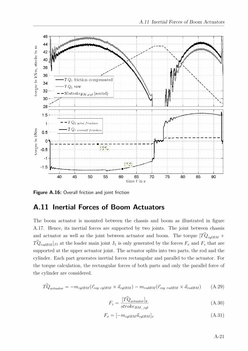
A.11 Inertial Forces of Boom Actuators
Figure A.16: Overall friction and joint friction
A.11 Inertial Forces of Boom Actuators
The boom actuator is mounted between the chassis and boom as illustrated in figure
A.17. Hence, its inertial forces are supported by two joints. The joint between chassis
and actuator as well as the joint between actuator and boom. The torque [ ~TQcylBM +~TQrodBM ]J1 at the loader main joint J1 is only generated by the forces Fx and Fz that are
supported at the upper actuator joint. The actuator splits into two parts, the rod and the
cylinder. Each part generates inertial forces rectangular and parallel to the actuator. For
the torque calculation, the rectangular forces of both parts and only the parallel force of
the cylinder are considered.
~TQactuator = −mcylBM (~rcog cylBM × ~acylBM ) − mrodBM(~rcog rodBM × ~arodBM) (A.29)
Fz =[ ~TQactuator]ystrokeBM_cyl
(A.30)
Fx = [−mcylBM~acylBM ]x (A.31)
A-21
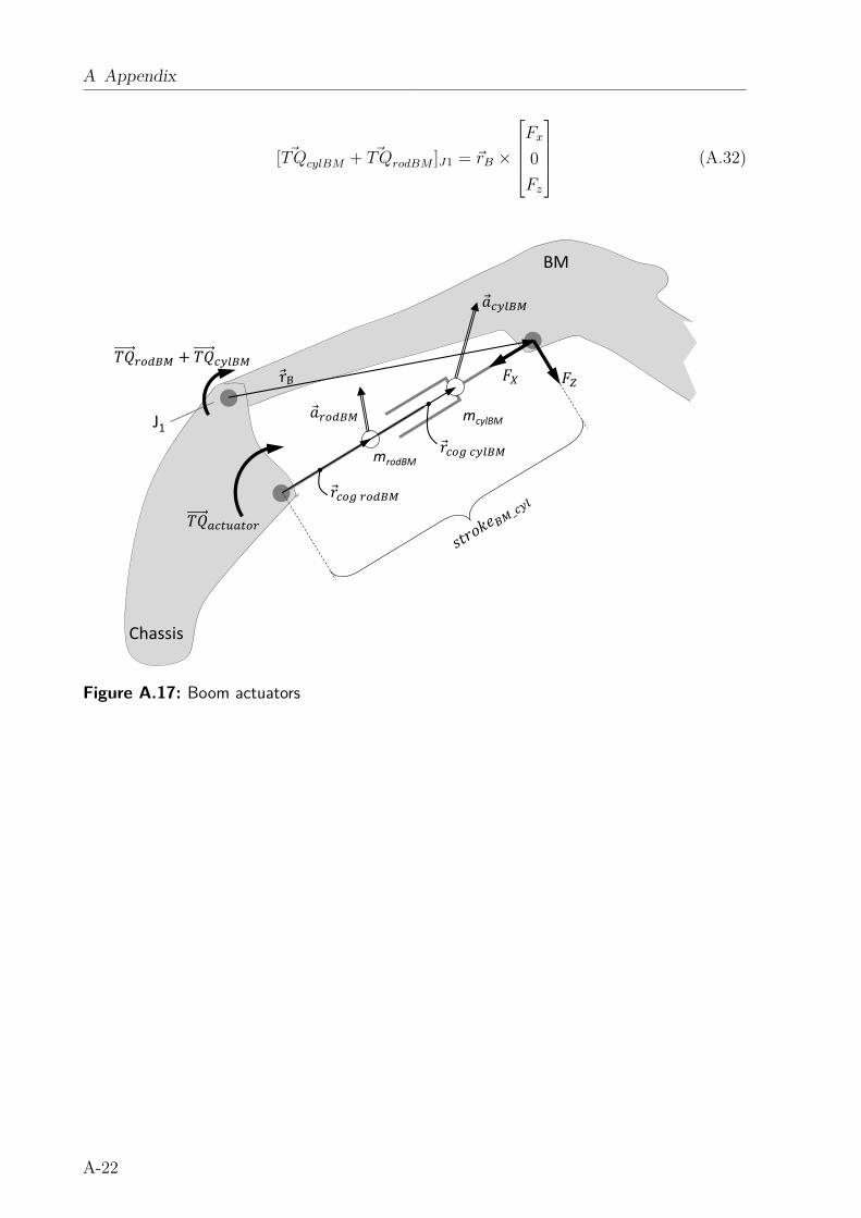
A Appendix
[ ~TQcylBM + ~TQrodBM ]J1 = ~rB ×
Fx
0
Fz
(A.32)
J1
BM
Chassis
mcylBM
mrodBM
��� ��
� �����
� � �� �� � � ��
��
�� �� + ��
Figure A.17: Boom actuators
A-22
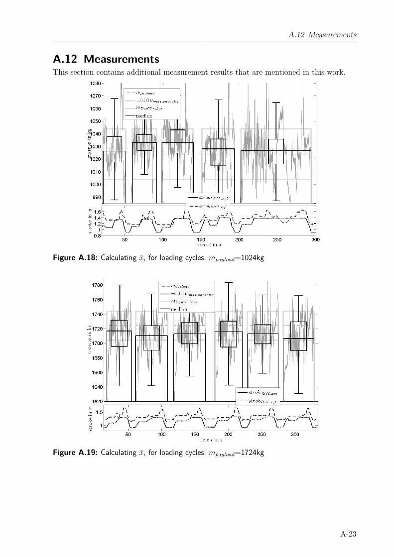
A.12 Measurements
A.12 MeasurementsThis section contains additional measurement results that are mentioned in this work.
Figure A.18: Calculating xi for loading cycles, mpayload=1024kg
Figure A.19: Calculating xi for loading cycles, mpayload=1724kg
A-23
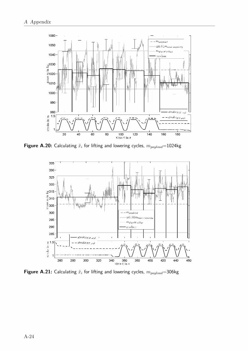
A Appendix
Figure A.20: Calculating xi for lifting and lowering cycles, mpayload=1024kg
Figure A.21: Calculating xi for lifting and lowering cycles, mpayload=306kg
A-24
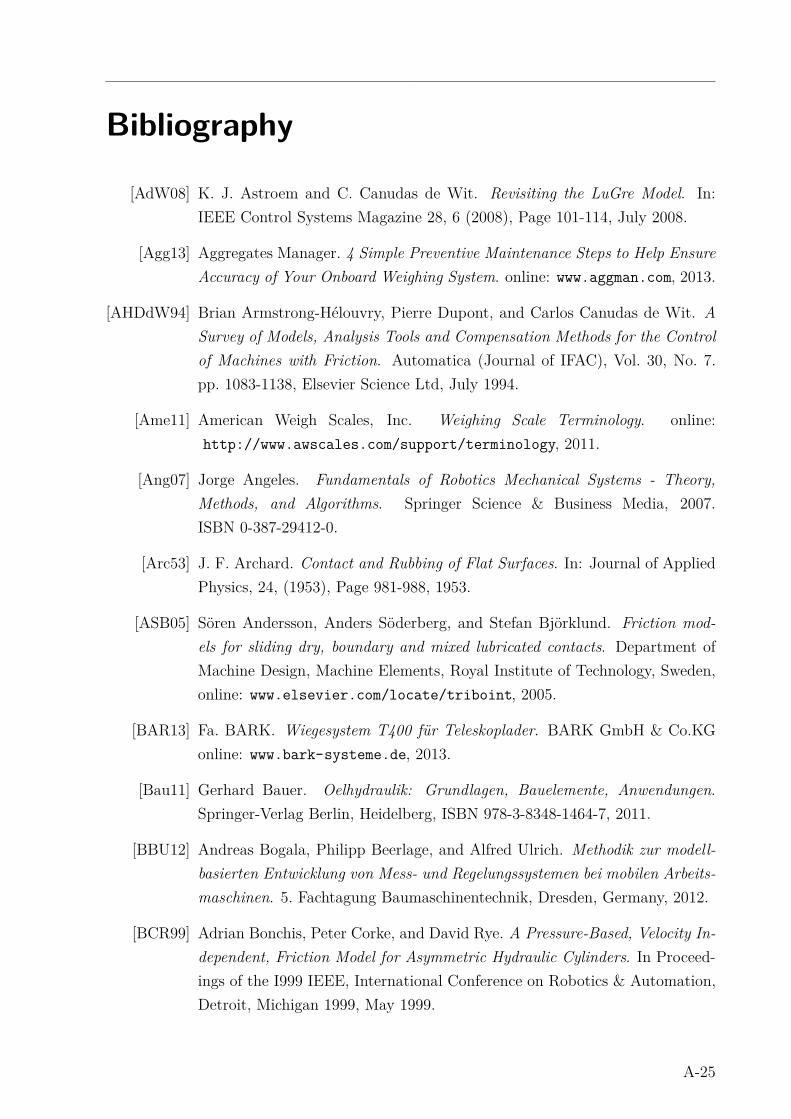
Bibliography
[AdW08] K. J. Astroem and C. Canudas de Wit. Revisiting the LuGre Model. In:
IEEE Control Systems Magazine 28, 6 (2008), Page 101-114, July 2008.
[Agg13] Aggregates Manager. 4 Simple Preventive Maintenance Steps to Help Ensure
Accuracy of Your Onboard Weighing System. online: www.aggman.com, 2013.
[AHDdW94] Brian Armstrong-Hélouvry, Pierre Dupont, and Carlos Canudas de Wit. A
Survey of Models, Analysis Tools and Compensation Methods for the Control
of Machines with Friction. Automatica (Journal of IFAC), Vol. 30, No. 7.
pp. 1083-1138, Elsevier Science Ltd, July 1994.
[Ame11] American Weigh Scales, Inc. Weighing Scale Terminology. online:
http://www.awscales.com/support/terminology, 2011.
[Ang07] Jorge Angeles. Fundamentals of Robotics Mechanical Systems - Theory,
Methods, and Algorithms. Springer Science & Business Media, 2007.
ISBN 0-387-29412-0.
[Arc53] J. F. Archard. Contact and Rubbing of Flat Surfaces. In: Journal of Applied
Physics, 24, (1953), Page 981-988, 1953.
[ASB05] Sören Andersson, Anders Söderberg, and Stefan Björklund. Friction mod-
els for sliding dry, boundary and mixed lubricated contacts. Department of
Machine Design, Machine Elements, Royal Institute of Technology, Sweden,
online: www.elsevier.com/locate/triboint, 2005.
[BAR13] Fa. BARK. Wiegesystem T400 für Teleskoplader. BARK GmbH & Co.KG
online: www.bark-systeme.de, 2013.
[Bau11] Gerhard Bauer. Oelhydraulik: Grundlagen, Bauelemente, Anwendungen.
Springer-Verlag Berlin, Heidelberg, ISBN 978-3-8348-1464-7, 2011.
[BBU12] Andreas Bogala, Philipp Beerlage, and Alfred Ulrich. Methodik zur modell-
basierten Entwicklung von Mess- und Regelungssystemen bei mobilen Arbeits-
maschinen. 5. Fachtagung Baumaschinentechnik, Dresden, Germany, 2012.
[BCR99] Adrian Bonchis, Peter Corke, and David Rye. A Pressure-Based, Velocity In-
dependent, Friction Model for Asymmetric Hydraulic Cylinders. In Proceed-
ings of the I999 IEEE, International Conference on Robotics & Automation,
Detroit, Michigan 1999, May 1999.
A-25
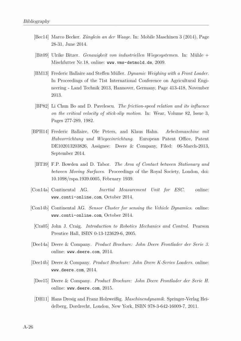
Bibliography
[Bec14] Marco Becker. Zünglein an der Waage. In: Mobile Maschinen 3 (2014), Page
28-31, June 2014.
[Bit09] Ulrike Bitzer. Genauigkeit von industriellen Wiegesystemen. In: Mühle +
Mischfutter Nr.18, online: www.vms-detmold.de, 2009.
[BM13] Frederic Ballaire and Steffen Müller. Dynamic Weighing with a Front Loader.
In Proceedings of the 71st International Conference on Agricultural Engi-
neering - Land Technik 2013, Hannover, Germany, Page 413-418, November
2013.
[BP82] Li Chun Bo and D. Pavelescu. The friction-speed relation and its influence
on the critical velocity of stick-slip motion. In: Wear, Volume 82, Issue 3,
Pages 277-289, 1982.
[BPH14] Frederic Ballaire, Ole Peters, and Klaus Hahn. Arbeitsmaschine mit
Hubvorrichtung und Wiegeeinrichtung. European Patent Office, Patent
DE102013203826, Assignee: Deere & Company, Filed: 06-March-2013,
September 2014.
[BT39] F.P. Bowden and D. Tabor. The Area of Contact between Stationary and
between Moving Surfaces. Proceedings of the Royal Society, London, doi:
10.1098/rspa.1939.0005, February 1939.
[Con14a] Continental AG. Inertial Measurement Unit for ESC. online:
www.conti-online.com, October 2014.
[Con14b] Continental AG. Sensor Cluster for sensing the Vehicle Dynamics. online:
www.conti-online.com, October 2014.
[Cra05] John J. Craig. Introduction to Robotics Mechanics and Control. Pearson
Prentice Hall, ISBN 0-13-123629-6, 2005.
[Dee14a] Deere & Company. Product Brochure: John Deere Frontlader der Serie 3.
online: www.deere.com, 2014.
[Dee14b] Deere & Company. Product Brochure: John Deere K-Series Loaders. online:
www.deere.com, 2014.
[Dee15] Deere & Company. Product Brochure: John Deere Frontlader der Serie H.
online: www.deere.com, 2015.
[DH11] Hans Dresig and Franz Holzweißig. Maschinendynamik. Springer-Verlag Hei-
delberg, Dordrecht, London, New York, ISBN 978-3-642-16009-7, 2011.
A-26
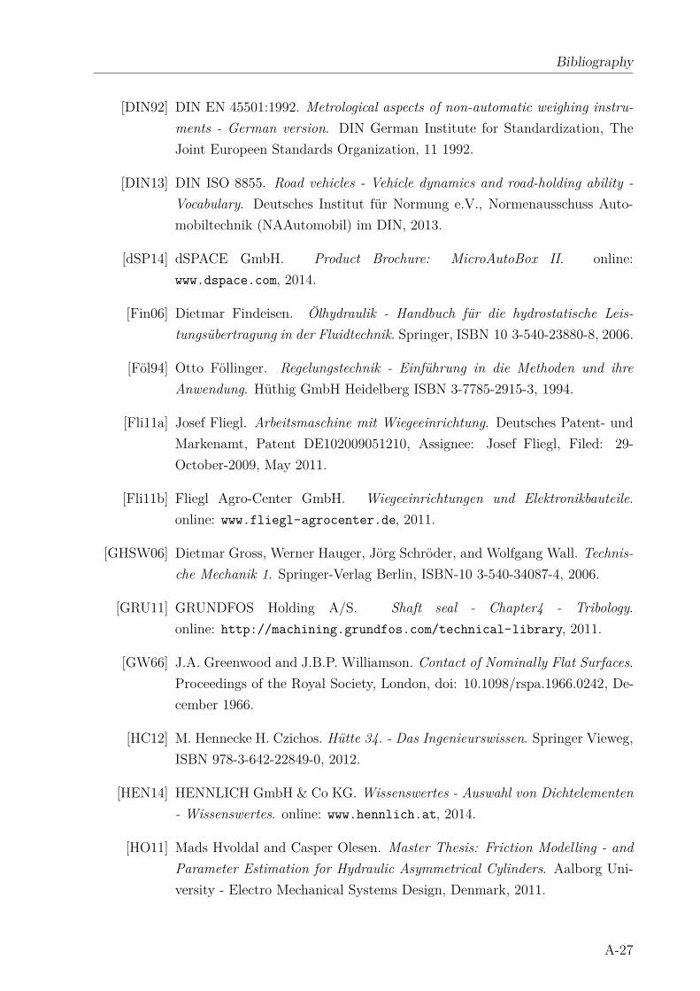
Bibliography
[DIN92] DIN EN 45501:1992. Metrological aspects of non-automatic weighing instru-
ments - German version. DIN German Institute for Standardization, The
Joint Europeen Standards Organization, 11 1992.
[DIN13] DIN ISO 8855. Road vehicles - Vehicle dynamics and road-holding ability -
Vocabulary. Deutsches Institut für Normung e.V., Normenausschuss Auto-
mobiltechnik (NAAutomobil) im DIN, 2013.
[dSP14] dSPACE GmbH. Product Brochure: MicroAutoBox II. online:
www.dspace.com, 2014.
[Fin06] Dietmar Findeisen. Ölhydraulik - Handbuch für die hydrostatische Leis-
tungsübertragung in der Fluidtechnik. Springer, ISBN 10 3-540-23880-8, 2006.
[Föl94] Otto Föllinger. Regelungstechnik - Einführung in die Methoden und ihre
Anwendung. Hüthig GmbH Heidelberg ISBN 3-7785-2915-3, 1994.
[Fli11a] Josef Fliegl. Arbeitsmaschine mit Wiegeeinrichtung. Deutsches Patent- und
Markenamt, Patent DE102009051210, Assignee: Josef Fliegl, Filed: 29-
October-2009, May 2011.
[Fli11b] Fliegl Agro-Center GmbH. Wiegeeinrichtungen und Elektronikbauteile.
online: www.fliegl-agrocenter.de, 2011.
[GHSW06] Dietmar Gross, Werner Hauger, Jörg Schröder, and Wolfgang Wall. Technis-
che Mechanik 1. Springer-Verlag Berlin, ISBN-10 3-540-34087-4, 2006.
[GRU11] GRUNDFOS Holding A/S. Shaft seal - Chapter4 - Tribology.
online: http://machining.grundfos.com/technical-library, 2011.
[GW66] J.A. Greenwood and J.B.P. Williamson. Contact of Nominally Flat Surfaces.
Proceedings of the Royal Society, London, doi: 10.1098/rspa.1966.0242, De-
cember 1966.
[HC12] M. Hennecke H. Czichos. Hütte 34. - Das Ingenieurswissen. Springer Vieweg,
ISBN 978-3-642-22849-0, 2012.
[HEN14] HENNLICH GmbH & Co KG. Wissenswertes - Auswahl von Dichtelementen
- Wissenswertes. online: www.hennlich.at, 2014.
[HO11] Mads Hvoldal and Casper Olesen. Master Thesis: Friction Modelling - and
Parameter Estimation for Hydraulic Asymmetrical Cylinders. Aalborg Uni-
versity - Electro Mechanical Systems Design, Denmark, 2011.
A-27
Bibliography
[Hol07] Uwe Hollburg. Maschinendynamik. Oldenbourg Wissenschaftsverlag GmbH,
ISBN 978-3-486-57898-0, 2007.
[Hon93] Josef Honerkamp. Klassische Theoretische Physik. Springer-Verlag Berlin,
Heidelberg, ISBN 3-540-55901-9, 1993.
[HSG99] Werner Hauger, Walter Schnell, and Dietmar Gross. Technische Mechanik 3
- Kinetik. Springer-Verlag Berlin Heidelberg NY,ISBN 3-540-66117-4, 1999.
[Ise06] Rolf Isermann, editor. Fahrdynamik - Regelung Modellbildung, Fahrerassis-
tenzsysteme, Mechatronik. Vieweg Verlag ISBN 978-3-8348-9049-8, 2006.
[KK87] Pradeep Khosla and Takeo Kanade. An Algorithm to Estimate Manipulator
Dynamics Parameters. Department of Electrical and Computer Engineering,
The Robotics Institute, Carnegie Mellon University, Pittsburgh, Pennsylva-
nia, March 1987.
[Käm12] Andreas Kämmerer. Development of a semi-automatic front loader with
weighing function by the example of the Fendt CARGO professional. VDI, In
Proceedings of the 70th International Conference on Agricultural Engineering
- Land Technik 2012, Karlsruhe, Germany, Page 63-68, 2012.
[Krä84] Erwin Krämer. Maschinendynamik. Springer-Verlag Berlin, Heidelberg,
Tokyo, ISBN 3-540-12541-8, 1984.
[Loa13] Trimble Loadrite. Product Brochure: Wheel loader scales L-Series.
online www.loadritescales.com, 2013.
[Loa14a] Loadrite. Case study: Accurate and profitable dairy farming. on-
line: http://www.loadritescales.com/loadrite-case-studies/
accurate-and-profitable-dairy-farming, 2014.
[Loa14b] Loadrite. Case study: Victorian dairy farm. online: http://www.
loadritescales.com/loadrite-case-studies/victorian-dairy-farm,
2014.
[Lun06] Jan Lunze. Regelungstechnik 2. Springer-Verlag Berlin, Heidelberg,
ISBN-13 978-3-540-32335-8, 2006.
[Lun08] Jan Lunze. Regelungstechnik 1. Springer-Verlag Berlin, Heidelberg,
ISBN 978-3-540-68907-2, 2008.
[Mar05] Dan Marghitu. Kinematic Chains and Machine Components Design. Elsevier
Academic Press, ISBN 0-12-471352-1, 2005.
A-28
Bibliography
[Mat10] MathWorks. Matlab Documentation. 1984-2010 The MathWorks, Inc, 2010.
[Mer14] Merkel Freudenberg Fluidtechnik GmbH. Merkel - Technisches Handbuch.
online: http://www.merkel-freudenberg.de/services/download-center/,
2014.
[MN13] Heinz Müller and Bernard Nau. Fachwissen Dichtungstechnik. online: www.
fachwissen-dichtungstechnik.de, 2013.
[NAS71] NASA SP-8063. Space Vehicle Design Criteria (Structures) - Lubrification,
Friction, and Wear. National Aeronautics and Space Administration, Wash-
ington, D.C., 1971.
[Nat02] National Conference on Weights and Measures - Rice Lake Weighing Systems.
NTEP & Handbook 44. NTEP, National Type Evaluation Program, online:
http://www.ncwm.net/, 2002.
[Nol06] Wolfgang Nolting. Grundkurs Theoretische Physik 1 - Klassische Mechanik.
Springer-Verlag Berlin, Heidelberg, New York, ISBN 3-540-34832-8, 2006.
[Oga02] Katsuhiko Ogata. Modern Control Engineering. Prentice Hall,
ISBN 0-13-043245-8, 2002.
[Ols96] Henrik Olsson. Control Systems with Friction. Department of Automatic
Control, Lund Institute of Technology, Sweden, 1996.
[Ove07] René M. Overney. Introduction to Tribology. Nanolab at the University of
Washington, online: http://depts.washington.edu/nanolab/ChemE554/
Summaries%20ChemE%20554/Introduction%20Tribology.htm, 2007.
[PFR14] PFREUNDT GmbH. Product Brochure: Die PFREUNDT Radladerwaa-
gen der pSerie. online: http://www.pfreundt.de/de/produkte/pSerie_
Radladerwaagen.php, 2014.
[Pro12a] Profi The Farm Machinery Magazine. Nicht am langen Arm heben. In: Profi
- Energie, 2 (2012), February 2012.
[Pro12b] Profi The Farm Machinery Magazine, Anja Böhrnsen. Volle Schaufeln
wiegen. In: Profi - Energie, 1 (2012), Page 78-83, January 2012.
[Pro14] Profi The Farm Machinery Magazin. Fendt Frontlader Cargo 4X/80 Profi:
Schlaue Schwinge. In: Profi, 4 (2014), Page 71 ff., April 2014.
A-29
Bibliography
[RDS08] RDS Technology Ltd. Product Manual: Loadmaster 8000 - On Board Weigh-
ing System. 2008.
[Sch07] Prof. Dr. Florian Scheck. Theoretische Physik 1 - Mechanik. Number ISBN
978-3-540-71377-7. Springer-Verlag Berlin, Heidelberg, 2007.
[Str02] Richard Stribeck. Die Wesentlichen Eigenschaften der Gleit- und Rollenlager.
Zeitschrift des Vereins Deutscher Ingenieure, Vol. 46, pp. 1341-1348, 1902.
[Tan06] Chin Pei Tang. Lagrangian Dynamic Formulation of a Four-
Bar Mechanism with Minimal Coordinates. Retrieved 2014 online:
http://nonholonomic.com/research.html, March 2006.
[TASLH08] Luc Le Tien, Alin Albu-Schäffer, Alessandro De Luca, and Gerd Hirzinger.
Friction Observer and Compensation for Control of Robots with Joint Torque
Measurement. In Proceedings of the IEEE/RSJ International Conference on
Intelligent Robots and Systems, Acropolis Convention Center Nice, France,
September 2008.
[Tre02] Peter Treue. PHD Thesis: Potenziale und Grenzen teilflächenspezifischer
N-Düngung in Schleswig-Holstein/Precision Agriculture. Inst. für Pflanzen-
bau und Pflanzenzüchtung, Lehrstuhl Acker- und Pflanzenbau, Christian-
Albrecht-Universität zu Kiel, Germany, 2002.
[Vei13] Veigroup.com. Case study Mongolia September 2013 Fuel Efficiency.
online: www.veigroup.com, September 2013.
[Vol14] Volvo CE. Product Brochure: Volvo Wheel Loader L45G and L50G. online
www.volvoce.com, 2014.
[Wat07] Holger Watter. Hydraulik und Pneumatik. Vieweg Verlag,
ISBN 978-3-8348-0190-6, 2007.
[WG08] Dieter Will and Norbert Gebhardt. Hydraulik - Grundlagen, Komponenten,
Schaltungen. Springer-Verlag Berlin, Heidelberg, ISBN 978-3-540-79534-6,
2008.
[Wil14] Wilhelm Stoll Maschinenfabrik GmbH. Product Brochure: Stoll FZ/Fs Pro-
filine. online: www.stoll-germany.com, 2014.
[Wis00] Ludger Wissing. Anordnung zum Wiegen von Nutzlasten. Deutsches Patent-
und Markenamt, Patent DE19901563A1, Assignee: Pfreundt GmbH, Filed:
16-January-1999, July 2000.
A-30
Bibliography
[WNB+06] Peter Wriggers, Udo Nackenhorst, Sascha Beuermann, Holger Spiess, and
Stefan Löhnert. Technische Mechanik kompakt - Starrkörperstatik Elasto-
statik Kinetik. Teubner Verlag, ISBN 10 3-8351-0087-4, 2006.
Student Projects
Immanuel Deepan Morais
Force and Torque Analysis on Front- and Wheel Loader with Hydraulic Cylinders using an
Optimal Controller Design for Trajectory Tracking, Master Thesis, 2014.
Christian Simonis
Userinterface und Statuserkennung für eine automatisierte Gewichtmessung am Traktor-
frontlader, Studienarbeit, 2014.
A-31


Curriculum Vitae
Frederic Ballaire
Berufstätigkeit
seit 04/2011 Wissenschaftlicher Mitarbeiter,
Lehrstuhl für Mechatronik in Maschinenbau und Fahrzeugtechnik
Technische Universität Kaiserslautern
03/2007 - 03/2011 Ingenieur, Volvo Construction Equipment Germany GmbH
Hochschulbildung
09/2000 - 02/2007 Studium Maschinenbau und Verfahrenstechnik
Schwerpunktfach: Konstruktionstechnik
Technische Universität Kaiserslautern
Abschluss: Diplom-Ingenieur
Diplomarbeit: Konzeption und Konstruktion eines
leistungsverzweigten Getriebes mit hydraulischer Kupplung
2. Studienarbeit: Entwicklung der Hinterbaukinematik
eines gefederten Mountainbikerahmens
1. Studienarbeit: Beschleunigungsmessungen
an der Gleitringdichtung einer Kreiselpumpe
Fachpraktikum: Keiper GmbH & Co.KG, Kaiserslautern
Versuch/Entwicklung, Prüfstandsoptimierung
Schulbildung
09/1990 - 06/2000 Rudi-Stephan-Gymnasium, Worms
Veröffentlichungen
Ballaire, F.; Müller, S.: Dynamic Weighing with a Front Loader. In Proceedings of
the 71st International Conference on Agricultural Engineering - LAND.TECHNIK 2013,
Hannover, Germany, November 2013, Page 413-418.
Sabzewari, K.; Ballaire, F.; Müller, S.: Energieeinsparpotenzial der Arbeitshy-
draulik durch die Elektrifizierung am Beispiel eines Frontladers. In Proceedings of the 72nd
International Conference on Agricultural Engineering - LAND.TECHNIK 2014, Berlin,
Germany, November 2014, Page 449-458.
Ballaire, F.; Peters, O.; Hahn, K.: Arbeitsmaschine mit Hubvorrichtung und Wiegeein-
richtung. European Patent Office, Patent DE102013203826, Assignee: Deere & Company,
Filed: 06-March-2013, September 2014.
Neustadt an der Weinstraße, 01.09.2015