DYNAMIC BEHAVIOUR AND INELASTIC

PERFORMANCE OF STEEL ROOF DECK DIAPHRAGMS

By Robert Massarelli Department of Civil Engineering and Applied Mechanics McGill University, Montréal, Canada August 2010 A thesis submitted to the Faculty of Graduate and Postdoctoral Studies in partial fulfillment of the requirements of the degree of Master of Engineering © Robert Massarelli, 2010

i

ABSTRACT

Modern building codes such as the NBCC 2005 require the use of capacity-based seismic design principles in which a ductile energy dissipating element, typically the bracing members of the vertical braced frames of the lateral force resisting system in single-storey structures, must be clearly identified. The diaphragm, used to transfer inertia loads to these vertical elements, must then be designed for the probable resistance of the braces. Furthermore, the code-proposed formula to calculate the fundamental period of vibration of single-storey structures does not account for the inherent flexibility of the diaphragm; whereas research has shown that accounting for this effect can result in longer building periods and, thereby, lower seismic forces and result in a more economical design. In-situ ambient vibration measurements have demonstrated that the period of single-storey structures may in fact be shorter than determined from structural models. It is believed, however, that ambient levels of loading are not representative of larger seismic motions. An experimental test frame mimicking the roof assembly of a single-storey steel structure was constructed in the laboratory. Corrugated steel sheets were fastened to the frame to complete the diaphragm assembly. Nine diaphragm specimens, with varying deck sheet thicknesses and orientations, fastened using typical construction methods, were tested dynamically to evaluate their stiffness, strength and ductility. Loading protocols, including one developed to induce inelastic deformations at the fasteners, were applied. Retrofit and repair strategies were subsequently evaluated in attempts to restitute the properties of the original specimens. From testing, it was determined that the stiffness of the diaphragm diminishes with increased excitation amplitude resulting in a longer fundamental period potentially beneficial for design.

ii

The design of a single-storey structure with a steel roof deck diaphragm, laterally supported by an eccentrically braced frame (EBF) was completed according to the NBCC 2005 and CSA S16-09 seismic provisions. When compared to a concentrically braced structure, it was determined that the overstrength of the eccentric brace system did not have as negative an impact on the diaphragm design. Furthermore, when the design incorporated the flexibility of the roof diaphragm, the structure had an increased drift demand compared to the case in which the roof diaphragm was considered rigid.

iii

RÉSUMÉ

Le Code National du Bâtiment du Canada (CNB 2005) exige l’utilisation de principes de conception basée sur la capacité dans laquelle un élément ductile capable de dissiper l’énergie, comme les diagonales des contreventements du système de résistance aux charges latérales pour les bâtiments de faible hauteur, doit être clairement identifié. Le diaphragme, qui sert à transférer les forces d’inertie à ces éléments verticaux, doit ensuite être conçu pour la résistance probable des contreventements. De plus, la formule proposée dans le CNB pour calculer la période des structures d’un seul étage ne tient pas compte de la flexibilité du diaphragme; alors que la recherche démontre que de tenir compte de cet effet peut donner lieu à une élongation de la période fondamentale de la structure et entraîner une baisse des forces sismiques et une conception plus économique. Des mesures in situ en vibrations ambiantes ont montré que la période des structures d’un seul étage peut en fait être plus courte que celle déterminée à partir de modèles structurels. On croit cependant que les niveaux de vibrations ambiantes ne sont pas représentatifs de grands mouvements sismiques. Un cadre d'essai expérimental imitant la toiture d'un bâtiment d’un seul étage a été construit en laboratoire. Des tôles ondulées ont été fixées au cadre pour compléter le montage. Neuf spécimens de diaphragme, fait de feuilles de tablier ayant différentes épaisseurs et orientations et étant fixées selon des méthodes de construction typiques, ont été testés dynamiquement afin d'évaluer leur rigidité, résistance et ductilité. Des protocoles de chargement, dont l’un développé spécifiquement pour induire des déformations inélastiques, ont été appliqués. Des stratégies de réparation ont ensuite été évaluées pour tenter de restaurer les propriétés originales. On a observé que la rigidité du diaphragme diminue avec une augmentation de l’amplitude d'excitation, ce qui sera possiblement bénéfique pour la conception de ces structures, à cause de l’allongement de la période fondamentale qui en résultera.

iv

La conception d’un bâtiment d'un seul étage avec un diaphragme en acier et un cadre à contreventement excentrique (CCE) à été complétée selon les clauses sismiques du CNB 2005 et de la norme CSA S16-09. La sur-résistance du système excentrique a eu un impact moins défavorable sur la conception du diaphragme que dans le cas d’un contreventement concentrique. De plus, les déformations inter-étages ont été plus importantes quand on tenait compte de la flexibilité du diaphragme comparé au cas où le diaphragme était considéré comme étant infiniment rigide.

v

ACKNOWLEDGEMENTS

There are many individuals to whom I owe a great amount of gratitude. First, I would like to thank both my supervisors Professor Colin A. Rogers and Professor Robert Tremblay for supplying the necessary guidance and encouragement to see me through to the very end of my two years of work on the project. Your patience and direction has allowed me to successfully achieve my goal, and for that I shall always be thankful. To all the hard-working members of the diaphragm team: John Franquet, Kishor Shrestha, David Ek, Derek Kozak and William Franquet, Thank you! For every nail and screw installed, mass hammered and decking sheet placed none of this work could have been accomplished without your help. Thank you to the technical staff of the structures laboratory at École Polytechnique, who at one time or another provided us with assistance and who were more than tolerant of our noise levels: Viacheslav Koval, Patrice Bélanger, Denis Fortier, Guillaume Cossette, Martin Leclerc, Marc Charbonneau, and Cédric Androuet. I would also like to recognize the financial support provided by the Natural Sciences and Engineering Research Council of Canada, the Steel Structures Education Foundation, the Canadian Sheet Steel Building Institute, and the member companies of the Vancouver Steel Deck Diaphragm Committee, as listed on the following pages; as well as the companies who supplied the materials required for our tests: Hilti, Canam, Sofab and Lainco. Finally, I would like to thank my family, Christine, and my friends for their support and constant encouragement. I would never have accomplished what I have without you, so thank you, again and again.

vi

VANCOUVER DIAPHRAGM COMMITTEE

Structural Engineering Companies Bianco Lam Consultants Bogdonov Pao Associates Ltd. Bush Bohlman CA Boom CWMM Glotman Simpson Consulting Engineers John Bryson & Partners Krahn Engineering Lang Structural Engineering Inc. Mainland Engineering Omicron Consulting Group PJB Engineering Ltd. Phoenix Structural Designs Ltd. RDJ Structural Pomeroy Engineering Read Jones Christoffersen Ltd. Reliable Equipment Rentals Siefken Engineering Ltd. Tabet Engineering Ltd. Thomas Leung Structural Engineering Inc. Weiler Smith Bowers Consulting Structural Engineers

vii

Decking Installers Rite-Way Metals Ltd. Continental Steel Ltd. The Beedie Group Teck Construction LLP Opus Building Canada Inc. Wales McLelland Construction Co. (1988) Ltd. ICC Integrated Cons Concepts Ltd. Prism Construction Ltd. Ventana Construction Corporation Rockwell Pacific Dominion Construction Company Inc. Contura Building Corp. Sun Life Financial (Real Estate Investment Division) Porte Realty Ltd. Overon Designs Architectural Design Sanford Designs Ltd. D Forcier Designs

viii

Table of Contents

Abstract .......................................................................................................................................... i

Résumé ........................................................................................................................................ iii

Acknowledgements .................................................................................................................. v

Vancouver Diaphragm Committee ..................................................................................... vi

List of Figures ........................................................................................................................... xii

List of Tables ........................................................................................................................... xiv

Chapter 1 - Introduction ......................................................................................................... 1 1.1 General Overview .................................................................................................................. 1 1.2 Statement of Problem .......................................................................................................... 3 1.3 Objectives .................................................................................................................................. 4 1.4 Scope and Methodology ...................................................................................................... 5 1.5 Outline ........................................................................................................................................ 6 1.6 Literature Review .................................................................................................................. 7 1.6.1 Seismic Design Guidelines ................................................................................... 7 1.6.1.1 National Building Code of Canada, 2005 .................................................. 7 1.6.1.2 Design of Steel Structures, CSA-S16 ........................................................ 10 1.6.2 Diaphragm Design Guidelines ......................................................................... 10 1.6.2.1 Steel Deck Institute Diaphragm Design Manual ................................. 10 1.6.2.2 CSSBI/Tri Services Technical Manual ..................................................... 12 1.6.2.3 Manual of Stressed Skin Diaphragm Design ........................................ 13 1.6.3 Past Research on Steel Roof Deck Diaphragms ....................................... 14 1.6.3.1 Analytical Studies ............................................................................................ 14 1.6.3.2 Laboratory and Field Studies ..................................................................... 17 1.6.3.3 Large-Scale Diaphragm Experiments, Phases I and II ...................... 21 1.7 Summary ................................................................................................................................ 23

Chapter 2 - Large-scale Dynamic Diaphragm Experiments .................................... 25 2.1 Test Overview ...................................................................................................................... 25 2.2 Experimental Setup and Testing .................................................................................. 25 2.2.1 Test Frame .............................................................................................................. 25 2.2.1.1 Steel Beams ........................................................................................................ 28 2.2.1.2 Open-web Steel Joists .................................................................................... 28 2.2.1.3 Frame Supports ................................................................................................ 29

ix

2.2.1.4 Additional Mass ................................................................................................ 31 2.2.2 Test Specimens ..................................................................................................... 34 2.2.2.1 Deck Sheets ........................................................................................................ 36 2.2.2.2 Deck Fasteners and Installation ................................................................ 37 2.2.2.3 Tailored Connections ..................................................................................... 43 2.2.2.4 Connection Repairs ........................................................................................ 47 2.2.2.5 Material Properties ......................................................................................... 49 2.2.3 Instrumentation and Data Acquisition ........................................................ 51 2.2.4 Experimental Loading Protocols ................................................................... 54 2.2.4.1 White Noise Signal .......................................................................................... 55 2.2.4.2 Sine Sweep Signal ............................................................................................ 55 2.2.4.3 Earthquake Signals ......................................................................................... 56 2.2.4.4 Sinusoidal Inelastic Signal ........................................................................... 57 2.3 Data Analysis and Methods ............................................................................................ 58 2.3.1 Data Modification and Filtering ..................................................................... 59 2.3.2 Natural Frequency ............................................................................................... 59 2.3.3 Resonance Plots .................................................................................................... 60 2.3.4 Damping ................................................................................................................... 61 2.3.5 Shear Force Calculation ..................................................................................... 62 2.3.6 Shear Force Hystereses ..................................................................................... 65 2.4 Test Results ........................................................................................................................... 66 2.4.1 Natural Frequency of Specimens ................................................................... 66 2.4.2 Damping Ratios ..................................................................................................... 68 2.4.3 Resonant Frequencies ........................................................................................ 69 2.4.4 Shear Force and Deformation Profiles ........................................................ 69 2.4.5 Inelastic Behaviour .............................................................................................. 71 2.5 Discussion of Results ......................................................................................................... 73 2.5.1 Diaphragm Shear Stiffness ............................................................................... 73 2.5.2 Damping ................................................................................................................... 77 2.5.3 Shear Force and Deformation Profiles ........................................................ 78 2.5.4 Diaphragm Shear Strength ............................................................................... 79 2.5.5 Diaphragm Inelastic Behaviour ...................................................................... 82 2.5.5.1 Failure Modes ................................................................................................... 82 2.5.5.2 Inelastic Deformation Capacity ................................................................. 87 2.5.6 Retrofit and Repair Strategies ........................................................................ 92 2.5.6.1 Nail and Screw Repairs ................................................................................. 92

x

2.5.6.2 Weld and Button-punch Repair and Retrofit ....................................... 93 2.5.6.3 Weld and Screw Repair ................................................................................. 94

Chapter 3 - Structural Design and Modelling ............................................................... 96 3.1 Overview of Task ................................................................................................................ 96 3.2 Building Location and Geometry .................................................................................. 96 3.3 Design Loads ......................................................................................................................... 98 3.3.1 Dead and Live Loads ........................................................................................... 99 3.3.2 Snow Loads ............................................................................................................. 99 3.3.3 Wind Loads .......................................................................................................... 100 3.3.4 Seismic Loads...................................................................................................... 100 3.4 Member Design ................................................................................................................. 104 3.4.1 Seismic Force Resisting System .................................................................. 105 3.4.2 Steel Roof Diaphragm ...................................................................................... 106 3.4.3 Gravity Resisting Members ........................................................................... 107 3.4.4 Wind Resisting Members ............................................................................... 108 3.5 Numerical Modelling ...................................................................................................... 109 3.6 Design Summary and Findings .................................................................................. 111 3.6.1 Fully Rigid System ............................................................................................ 112 3.6.2 Diaphragm with SDI Stiffness ...................................................................... 114 3.6.3 Diaphragm with 70% of SDI Stiffness ....................................................... 115 3.7 Modelling Conclusions ................................................................................................... 123

Chapter 4 - Conclusions and Recommendations ....................................................... 125 4.1 Summary ............................................................................................................................. 125 4.2 Conclusions ........................................................................................................................ 125 4.2.1 Test Program ...................................................................................................... 125 4.2.2 Single-Storey Building Design ...................................................................... 127 4.3 Recommendations for Future Work ........................................................................ 128

References .............................................................................................................................. 130

Appendix A : SDI Shear Strength and Stiffness Calculations ................................ 135

Appendix B : Testing Protocol Checklist ..................................................................... 157

Appendix C : Frequency Results from White Noise Testing for New Diaphragm Specimens ............................................................................................................................... 174

xi

Appendix D : Frequency Results from White Noise Testing for Repaired Diaphragm Specimens ........................................................................................................ 184

Appendix E : Damping Ratios .......................................................................................... 192

Appendix F : Sine Sweep Resonance Curves .............................................................. 195

Appendix G : Shear Force and Deformation Profiles for New Diaphragm Specimens ............................................................................................................................... 197

Appendix H : Shear Force and Deformation Profiles for Repaired Diaphragm Specimens ............................................................................................................................... 216

Appendix I : Shear Force vs. Mid-Span Displacement Hystereses for New Diaphragm Specimens ........................................................................................................ 231

Appendix J : Shear Force vs. Mid-Span Displacement Hystereses for Repaired Diaphragm Specimens ........................................................................................................ 235

Appendix K : Fastener and Mass Observation Sheets for Inelastic Test .......... 239

Appendix L : Stiffness, Strength, and Inelastic Property Graphs for all New Phase I, II and III Diaphragm Specimens ..................................................................... 370

xii

LIST OF FIGURES

Figure 1.1 – Single-storey building and representation of capacity based design of the bracing members (top) and the roof diaphragm (bottom) (Rogers & Tremblay, 2010) .............................................................................................................................................................. 2 Figure 1.2 – Interior panel force distribution (Luttrell, 2004) ........................................... 11 Figure 1.3 – 3D model and measured fundamental periods (Tremblay et al, 2008a) ....................................................................................................................................................................... 16 Figure 2.1 – Diaphragm test frame during assembly .............................................................. 26 Figure 2.2 – Test frame setup for Layout I (top) and II (bottom) ...................................... 27 Figure 2.3 – Diaphragm connection to the beam flange and HSS shear connector .... 28 Figure 2.4 – Actuator (black) installed on reaction column (burgundy) ........................ 29 Figure 2.5 – Connection between the actuator’s rod end and the end beam extension ....................................................................................................................................................................... 30 Figure 2.6 – Frame supports: HSS rocker (left) and steel-plate roller (right) .............. 31 Figure 2.7 – Typical 20-mass layout on a deck sheet .............................................................. 31 Figure 2.8 – Additional mass in the form of welded steel plates ....................................... 32 Figure 2.9 – P-3615 (top) and P-3606 (bottom) steel deck profiles (Canam Group Inc., 2006) ................................................................................................................................................. 36 Figure 2.10 – Mechanical fasteners before and after installation ...................................... 38 Figure 2.11 – Power-actuated fastening tool for nails (left) and screwdriver with stand-up handles (right) ..................................................................................................................... 38 Figure 2.12 – Non-mechanical sidelap fasteners during and after installation ........... 40 Figure 2.13 – Fastener pattern configurations (Canam Group Inc., 2007) .................... 41 Figure 2.14 – Tailored fastener pattern for DIA18 .................................................................. 46 Figure 2.15 – Damaged (D) and new (N) connectors: nails, welds and screws ........... 48 Figure 2.16 – Screwed steel strip repair of button-punched connections ..................... 49 Figure 2.17 – Data acquisition system .......................................................................................... 51 Figure 2.18 – Potentiometer and accelerometer (left) and velocity transducer (right) ....................................................................................................................................................................... 52 Figure 2.19 – LVDT and Teflon support for sidelap slip measurements ........................ 52 Figure 2.20 – Instrumentation setup for Layout I (top) and II (bottom) tests ............. 53 Figure 2.21 – Dynamic experimental loading protocols ........................................................ 54 Figure 2.22 – Displacement and acceleration record for Loma Prieta signal (SS1) ... 56 Figure 2.23 – Displacement and acceleration record for Northridge signal (SS3) ..... 56 Figure 2.24 – Displacement record for sinusoidal inelastic signal (SS2) ....................... 57

xiii

Figure 2.25 – Sine sweep resonance plot example .................................................................. 61 Figure 2.26 – Tributary areas for mass determination of Layout II ................................. 62 Figure 2.27 – Fundamental period as a function of the root mean square of the response acceleration for DIA16 ..................................................................................................... 66 Figure 2.28 – Comparison of experimental and predicted stiffness at varying levels of the predicted strength for DIA16 ............................................................................................... 68 Figure 2.29 – Free decay and damping envelope plot of DIA17 ......................................... 68 Figure 2.30 – Resonance curve plot of DIA15R ......................................................................... 69 Figure 2.31 – Shear force and deformation profile plot of DIA11 ..................................... 70 Figure 2.32 – Shear force time history plot for DIA11, SS1 signal ..................................... 70 Figure 2.33 – Shear force vs. displacement hystereses at mid-span (top) and end panel (bottom) of DIA11 ..................................................................................................................... 72 Figure 2.34 – Measured ambient shear stiffness vs. SDI prediction ................................. 75 Figure 2.35 – Measured experimental shear stiffness vs. SDI prediction ...................... 76 Figure 2.36 – Average normalized shear force and deformation profiles for elastic and inelastic tests .................................................................................................................................. 78 Figure 2.37 – Measured vs. predicted shear strength for all Phase III specimens ...... 81 Figure 2.38 – Typical fastener failure modes ............................................................................. 84 Figure 2.39 – Shear force vs. deformation hystereses and inelastic damage patterns for a) DIA11, b) DIA14, c) DIA17 and d) DIA18 ........................................................................ 85 Figure 2.40 –Damage distribution during inelastic test ........................................................ 86 Figure 2.41 – Ultimate shear strain for all Phase I, II and III specimens ........................ 89 Figure 2.42 – Shear force vs. displacement hysteresis for DIA15R .................................. 90 Figure 2.43 – Normalized energy dissipated for all Phase III specimens ....................... 91 Figure 2.44 – Schematic of flexible end panel for DIA18R .................................................... 93 Figure 2.45 – End panel hystereses of DIA10R, DIA11 and DIA15R ................................ 94 Figure 2.46 – Damage distribution for DIA13 (left) and DIA19 (right) ........................... 95 Figure 3.1 – Design spectrum for Abbotsford, BC (Site class C) ......................................... 97 Figure 3.2 – Roof plan and wall elevation of single-storey building ................................. 98 Figure 3.3 – Representation of inelastic beam rotation ...................................................... 106 Figure 3.4 – 3D model of the structure ...................................................................................... 110

xiv

LIST OF TABLES

Table 1.1 – Phase I and II diaphragm specimen configurations (Franquet, 2010) .... 22 Table 2.1 – Total weight of test setup ............................................................................................ 33 Table 2.2 – Weight of individual components (Layout I) ...................................................... 33 Table 2.3 – Weight of individual components (Layout II) .................................................... 33 Table 2.4 – Phase III diaphragm test specimen configurations .......................................... 35 Table 2.5 – Fastener designations for Phase III tests .............................................................. 37 Table 2.6 – Total and average values for Phase III welded specimens ............................ 39 Table 2.7 – Phase III SDI method strength and stiffness predictions ............................... 42 Table 2.8 – Frame fastener patterns and average strengths for DIA18 .......................... 45 Table 2.9 – Summary of Specimen Repair/Retrofit Methods .............................................. 48 Table 2.10 – Summary of material properties ........................................................................... 50 Table 2.11 – List of sinusoidal inelastic protocols ................................................................... 58 Table 2.12 – Specimen mass per tributary area for Layout I ............................................... 63 Table 2.13 – Specimen mass per tributary area for Layout II ............................................. 64 Table 2.14 – Representation of connector damage ................................................................. 72 Table 2.15 – Diaphragm stiffness at various levels of excitation ....................................... 74 Table 2.16 – Diaphragm damping ratios ...................................................................................... 78 Table 2.17 – Predicted and measured diaphragm shear strength .................................... 80 Table 2.18 – Summary of inelastic properties ........................................................................... 89 Table 3.1 – Initial assumptions and design values ................................................................ 102 Table 3.2 – Design forces in the braced bays ........................................................................... 104 Table 3.3 – Member design summary ........................................................................................ 109 Table 3.4 – Design summary with rigid roof diaphragm (2Ta, 2.5Ta and 3Ta) .......... 117 Table 3.5 – Design summary with rigid roof diaphragm (unbounded period) ......... 118 Table 3.6 – Design summary with flexible roof diaphragm (G’SDI) (2Ta, 2.5Ta and 3Ta) .................................................................................................................................................................... 119 Table 3.7 – Design summary with flexible roof diaphragm (G’SDI) (unbounded period) ..................................................................................................................................................... 120 Table 3.8 – Design summary with flexible roof diaphragm (0.7*G’SDI) (2Ta, 2.5Ta and 3Ta) ........................................................................................................................................................... 121 Table 3.9 – Design summary with flexible roof diaphragm (0.7*G’SDI) (unbounded period) ..................................................................................................................................................... 122

1

Chapter 1 - INTRODUCTION

1.1 General Overview The satisfactory performance of a structure during a seismic event is of extreme importance in order to avoid potential collapse and to preserve the safety of its occupants. As such, the 2005 version of the National Building Code of Canada (NBCC) (NRCC, 2005) has developed more stringent seismic design guidelines, where ground motions with a probability of exceedance of 2% in 50 years need to be considered for design, as opposed to 10% in the previous 1995 edition (NRCC, 1995). Along with the increased seismic requirements, the Canadian building code and Limit States Design of Steel Structures standard (CSA, 2009) necessitate the use of capacity based design principles for moderate ductility (type MD) and limited ductility (type LD) concentrically braced frames. This requires that a particular element of the seismic force resisting system (SFRS), typically the bracing members of the vertical braced frames, be selected as a fuse and detailed to undergo inelastic deformations through yielding. All other members of the SFRS are then designed for the probable resistance of these braces. As mentioned, the current convention in type MD and LD single-storey steel frame construction is to design and detail the lateral braces as the fuse elements. The diaphragm, which is typically constructed of corrugated cold formed steel panels, and relied upon to support the gravity loads as well as to transfer lateral wind and seismic loads at the roof level to the vertical bracing, must then be detailed for the probable strength of these members as shown in Figure 1.1. Additionally, the calculated fundamental periods of single-storey structures lengthen when accounting for the expected in-plane flexibility of steel roof deck diaphragms, beyond the upper bound limit imposed by the NBCC (NRCC, 2005), resulting in larger than necessary seismic forces. The compounded effects of the increased seismic loads, capacity design requirements, and period limitation has largely contributed

2

to designs incorporating thicker decks with more closely spaced connectors, which has negatively impacted the construction costs of single-storey structures, especially those found in zones of high seismicity such as the Ottawa and St. Lawrence valleys and the western regions of British Columbia. To circumvent some of these issues one possibility is to allow designers to incorporate the inherent in-plane flexibility present in the roof diaphragm when calculating the fundamental period of a structure, as a longer period would result in lower seismic forces for design. Past studies, such as those completed by Lamarche (2005) and Tremblay et al. (2008a) show contradictions as the periods obtained from in-situ ambient vibration measurements on a single-storey structure did not correspond to the periods from a basic structural model of the same building. An alternative design approach, shown in Figure 1.1, would be to select the steel roof deck diaphragm as the main energy dissipating element of the SFRS; however this approach has yet to be fully validated. In order to properly characterize the dynamic properties of such systems, further research, such as is presented in this thesis, is necessary.

Figure 1.1 – Single-storey building and representation of capacity based design of the bracing members (top) and the roof diaphragm (bottom) (Rogers & Tremblay, 2010)

Steel DeckUnits (typ.)

a)

VerticalX Bracing

(typ.)

Chord (typ.)

Collector(typ.)

V

CollectorElements

BracingConnections

Foundations

Collector Collector

RoofDiaphragm

BracingMembers(Inelastic)

AnchorBolts

VV

Collector Collector

CollectorElements

RoofDiaphragm(Inelastic)

BracingMembers

AnchorBolts

BracingConnections

Foundations

VV

)

3

1.2 Statement of Problem The recent shift towards capacity based design provisions of the NBCC 2005 (NRCC, 2005), combined with the increased seismic forces to be considered in design, have had a negative impact on the design of single-storey structures in Canada. Typically supported laterally by a vertical bracing system, which is also used as the main energy dissipating element of the SFRS in type MD and LD concentrically braced frame systems, the roof diaphragm must be designed to remain elastic given the probable force developed in the braces. The impact is even more profound if a tension-compression bracing system is used. In this type of structural system, the design of the brace is usually governed by their slenderness in compression and hence a much greater tension reserve strength must be considered when selecting the surrounding protected elements such as the roof diaphragm. The result is a thicker than necessary deck, with more closely spaced connections, and an increased cost of construction. Another point of contention is that structural codes such as the NBCC 2005 (NRCC, 2005) provide empirical formulas that do not account for the flexibility of the diaphragm when determining the fundamental period of the building. Instead, the formulas are determined considering the stiffness of the lateral bracing elements. Should the diaphragm flexibility be considered in obtaining the period, lower seismic forces and a less costly structure may result. Furthermore, Tremblay and Rogers (2005) showed that using the diaphragm as the fuse element could in fact provide a more economical design as the diaphragm design forces are reduced. Using the diaphragm in this manner, however, requires that the connections undergo significant inelastic deformations and will invariably incur damage. Retrofit and repair strategies for currently constructed structures have not been examined, but would be necessary in order to improve the strength and stiffness of a diaphragm prior to an earthquake, or to recuperate these same properties following a seismic event.

4

Previous research completed by Essa (2001), Martin (2002) and Yang (2003) has examined diaphragm behaviour using specimen configurations representative of North American construction, however a cantilever setup allowed for only uniform shear loading to be applied to the specimens. Dynamic diaphragm tests on large scale specimens that emulate actual diaphragm configuration and boundary conditions while incorporating loading protocols representative of what would be expected during a strong ground motion seismic event have never been undertaken. Testing of this nature would allow for the evaluation of diaphragm properties, such as the strength and stiffness under conditions approaching actual seismic events, which may differ from the properties obtained from in-situ ambient measurements. Finally, diaphragm design methods, such as the SDI (Luttrell, 2004) do not account for the effects of deck sheet orientation when determining the diaphragm’s strength and stiffness properties. By undertaking representative tests and varying the sheet direction with respect to the load, information can be obtained to account for this currently neglected effect. 1.3 Objectives The general objective of this research project is to generate data that could lead to more economically attractive seismic design and retrofit-repair strategies that take into account the flexibility and ductility of the steel roof deck diaphragm for single-storey buildings. The specific objectives of the research are as follows:

• Determine and evaluate the dynamic properties of steel roof deck diaphragms through experimental testing. • Devise and evaluate experimentally, retrofit and repair strategies for existing building roof diaphragms.

5

• Compare the behaviour of the diaphragms under different orientations of applied loading. • Experimentally assess the inelastic seismic response of steel deck diaphragms in the context of taking advantage of the diaphragm acting as the fuse element in the seismic force resisting system (SFRS). • Comparison of design strategies for a single-storey structure laterally supported by an eccentrically braced frame using different assumptions of diaphragm stiffness.

1.4 Scope and Methodology The research involved dynamic testing of large-scale cold-formed steel roof deck diaphragm specimens as part of Phase III of an on-going test program initiated in 2007. The nine diaphragm configurations in Phase III were selected to replicate the thicknesses and connectors that are commonly found in single-storey construction in North America, as well as to expand upon the tests examined by Franquet (2010) in Phases I and II. The specimens included: thicknesses of 0.76 mm (22 gauge), 0.91 mm (20 gauge) and 1.21 mm (18 gauge) decks, considering a variety of nailed, screwed, welded and button-punch connection configurations. As well, the orientation of the deck sheets was varied in order to evaluate the influence of a change in direction of the applied force. Dynamic characteristics of the diaphragms such as the fundamental period, damping ratio, deformed shape, shear force profile and load carrying capacity were extracted from the tests. Each specimen was also tested in its repaired state to evaluate the effectiveness of various repair strategies in restoring the original dynamic properties. Additionally, one diaphragm specimen connected using welds and button-punches was retrofitted using nails and screwed steel strips

6

before testing. Comparisons of the evaluated strength and stiffness for every test were made with their respective Steel Deck Institute (SDI) predictions (Luttrell, 2004). The design of a single-storey structure situated in Abbottsford, British Columbia was performed. The building, constructed with an eccentrically braced frame was designed for the following three separate assumptions of diaphragm shear stiffness: a rigid system, stiffness as determined using the SDI method, and 70% of the SDI stiffness. Furthermore, the design was completed for each of the stiffness assumptions using various upper limits of the fundamental period for the calculation of the seismic design forces, namely 2Ta, 2.5Ta, 3Ta and an unbounded period. 1.5 Outline An overview of the research project is given in this chapter. It is followed by a literature review which contains knowledge on the topics of seismic design as well as past research involving steel roof deck diaphragms. Chapter 2 is devoted to the explanation of the experimental program. It includes an overview of the diaphragm specimens, test methods, loading protocols and data analysis, including presentation and discussion of the results. Chapter 3 presents information related to the seismic design of a single-storey structure laterally supported by an eccentrically braced frame (EBF). Finally, conclusions of the work have been provided in Chapter 4. A summary of the major findings is provided as well as suggestions for future research.

7

1.6 Literature Review The following section presents pertinent information that applies to the study of steel roof deck diaphragms. It contains an overview of seismic and diaphragm design guidelines, as well as a summary of selected past research related to this topic.

1.6.1 Seismic Design Guidelines

1.6.1.1 National Building Code of Canada, 2005 The National Building Code of Canada (NBCC) (NRCC, 2005) is the governing document for the evaluation of structural loads acting on a building and all its members. A summary of the main excerpts as related to seismic design are presented in this section. In order to resist the effects of seismic loading, the NBCC states that a structure must have a clearly defined load path, which is capable of transferring the inertial forces developed during an earthquake to the supporting ground. Additionally, there must be a clearly defined seismic force resisting system (SFRS), which is responsible to accept the full effects of any seismic loading. Other structural elements not part of the SFRS are then required to behave elastically, or alternatively, if they are capable of exhibiting sufficient non-linear capacity, are allowed to undergo some inelastic deformation. To determine the forces to be resisted by the SFRS, the NBCC allows two pre-qualified methods depending on the classification of the structure, which may be either regular, or irregular, in which the structure contains any number of structural irregularities, such as those involving stiffness, mass, and geometry. The two methods are the equivalent static force procedure (ESFP), which may be used only for regular structures, or irregular structures that satisfy certain restrictions, and a dynamic analysis. The equivalent static force procedure is presented in Equation 1.1.

8

(1.1) Minimum lateral earthquake load force Spectral acceleration values at the fundamental lateral period A factor to account for the effect of higher modes Importance factor of the structure Seismic weight of the building Ductility-related force modification factor Overstrength-related force modification factor Certain restrictions are set on the value of the seismic base shear, V, such that it cannot be lower than a formula-defined minimum value for all systems, and need not be higher than a defined maximum for systems in which Rd ≥ 1.5. In multi-storey buildings, the total lateral force is then distributed such that a specified amount is concentrated at the top of the building, due to higher mode effects, with the remainder being distributed over the height according to a defined empirical distribution. Additional loads due to torsional effects are also to be considered in evaluating the forces acting on a structure. These torsional moments are caused by either or both of eccentricities between the centres of mass and rigidity, and accidental eccentricities equal to 10% of the plan dimension of the building perpendicular to the seismic loading. As well, limits are defined for the deflections and drift of the structure, no matter which analysis procedure is used. These limits depend on the importance of the structure, and are equal to 0.025 times the inter-storey height for the majority of structures. In Equation 1.1, the lateral period, Ta, is selected by either a formula, or with the use of a structural model. For example, in a structure for which the SFRS is that of a braced-frame, the formula for determining the period is:

9

0.025 (1.2) Height of the building in metres Alternatively, if the period is determined using a structural model, the NBCC allows it to be taken no larger than twice the value of Ta. Spectral response acceleration values are listed in the NBCC for individual cities, and are based on a 2% probability of exceedance in 50 years. These are transformed into design values by adjusting them according to Clause 4.1.8.4.6 (NRCC, 2005), using Fa and Fv values that represent the acceleration and velocity-based site coefficients determined by the ground classification of the site. The ductility and overstrength force modification factors are also defined in the NBCC, and are listed according to the type of SFRS, with any particular height restrictions that may apply. As an alternative to the equivalent static force procedure, the NBCC permits designers to also perform a linear dynamic analysis, or a nonlinear dynamic analysis. The dynamic analysis procedures can be beneficial as they may allow for a larger value of the fundamental period to be used for the calculation of the seismic actions up to a specified maximum. However, the code specifies that the results from dynamic analysis be scaled such that the total earthquake load is the same as, or equal to 80% of, in the case of regular structures, the force, V, from the equivalent static force procedure. In addition, a large degree of detail must be accounted for in the structural model to be representative of the actual building. Finally, specific design provisions as they apply to diaphragms are also included in the NBCC, where it is stated that diaphragms are to be designed to remain elastic. Additionally, the design of diaphragms should account for the larger of the forces due to either of the following cases: loads as

10

determined by the static force procedure or by dynamic analysis, increased to reflect the lateral load carrying capacity of the SFRS plus additional forces due to the transfer of forces between elements of the SFRS, or a minimum force equal to the design-based shear divided by the total number of storeys. More detailed examinations of the NBCC 2005 seismic design provisions, as well as a description of the force modification factors can be found in the literature by Humar and Mahgoub (2003), Humar et al. (2003), Heidebrecht (2003) and Mitchell et al. (2003). 1.6.1.2 Design of Steel Structures, CSA-S16 The Canadian Standards Association CSA-S16 Standard (2009) is the governing document for steel structures in Canada. In terms of seismic design provisions, the standard follows the principles of capacity based design, and provides details for all steel seismic force resisting systems for which energy dissipation capability is required, consistent with the ductility and overstrength related factors set forth by the NBCC 2005 (NRCC, 2005). With respect to diaphragms, the commentary on CSA-S16 provided by the Canadian Institute of Steel Construction (CISC, 2010), mentions that diaphragms of buildings of the Conventional Construction category (type CC, Rd = 1.5 and Ro = 1.3) and for which the connections have shown by testing to exhibit a ductile mode of failure may be designed for forces corresponding to RdRo = 1.95. For diaphragms in which the connections do not exhibit this type of behaviour, the design should consider seismic forces obtained with RdRo = 1.3. 1.6.2 Diaphragm Design Guidelines

1.6.2.1 Steel Deck Institute Diaphragm Design Manual The Steel Deck Institute (SDI) design method (Luttrell, 2004) is based on numerous tests completed since 1965 at the University of West Virginia (Luttrell, 1981), and applies to decks that range in thickness from 0.36 mm to

11

1.63 mm, and vary in depth from 14 mm to 36 mm, which cover the most commonly found deck profiles used in North America. The SDI Manual addresses factors that affect the in-plane strength and stiffness of a diaphragm assembly, which are summarized in the following paragraphs. The SDI has found the shear strength of a diaphragm to be controlled by the lowest of the following resistances: 1.) Shear strength of the connections a. Based on the limitations of the fasteners at an edge panel b. Based on the limitations of the fasteners at an interior panel 2.) Localised panel buckling at the location of a corner fastener 3.) Shear buckling of the diaphragm between vertical supports The equations developed to determine the shear strength of the connections, as well as the local panel buckling are largely based on the capacities of the deck-to-frame connections and sidelap connections, represented by Qf and Qs respectively. Used in conjunction with the assumption that fasteners located farthest from the centreline of a panel are fully stressed, and that a linear stress distribution applies, force diagrams can be developed to obtain the corresponding resistance equations per unit length of a panel. An example force distribution is shown in Figure 1.2 for a typical interior panel.

Figure 1.2 – Interior panel force distribution (Luttrell, 2004)

12

The design shear stiffness of a diaphragm can be developed by initially considering the expression for the stiffness of a flat plate. This equation is then expanded upon to include adjustments that take into consideration the reduced stiffness imparted by the geometry of the cross section, warping distortion of the flutes, and flexibility of the connections. The final SDI design expression for stiffness is shown in Equation 1.3 2 1 (1.3) Modulus of elasticity Sheet thickness Poisson’s ratio Developed flute width per width Panel corrugation pitch Factor to account for the number of spans within the full panel length Warping coefficient Slip coefficient In order to calculate the properties of a diaphragm according to the SDI method, the strengths and flexibilities of the different fasteners must be determined. To simplify this process, the SDI has provided equations that are based on a large number of tests for typical diaphragm connectors, including welds, screws, power driven fasteners and button-punches. Such equations can be found in Chapter 4 of the SDI design manual (Luttrell, 2004).

1.6.2.2 CSSBI/Tri Services Technical Manual In Canada, the Canadian Sheet Steel Building Institute guide (CSSBI, 2006) proposes both the SDI method and the Tri-Services method (1982) for the design of diaphragms. The latter is similar to the SDI method and is based on numerous tests through which empirical equations were developed for both diaphragm strength and diaphragm stiffness determination. Like the SDI method, its equations are independent of the orientation of the deck sheets,

13

however the method is limited to diaphragms that are connected to the frame through welds and are fastened at their sidelaps using button-punches or seam welds. Using this procedure, the shear resistance of the diaphragm is determined by the lesser of elastic shear buckling and connection failure, which is based on a combination of the shear resistance of the welded frame fasteners and the sidelap connections. Furthermore, an additional limit is imposed in order to ensure that the shear resistance of the sidelap fasteners is not exceeded. When considering stiffness, a flexibility factor, F, is calculated for a diaphragm assembly. The flexibility factor includes contributions from three effects, which are: the flexibility of the diaphragm acting as a flat plate, changes in flexibility and warping with regards to the number of spans, and the flexibility due to sheet and fastener deformations. Both the SDI and Tri-Services methods treat the diaphragm and the perimeter structural members as being analogous to a deep girder. Here, with the eave members acting as the flanges and the diaphragm as the web, shear deflections play an important role in total building lateral deflection calculations. The flexural deformations of the roof assembly are assumed resisted by the perimeter members, while the shear deformation depends directly on the in-plane shear stiffness of the deck and its connections. 1.6.2.3 Manual of Stressed Skin Diaphragm Design Stressed skin design, developed by Davies and Bryan (1982) is the European approach to the design of diaphragm assemblies. Similar to the other SDI and Tri-Services methods, this approach focuses on determining the in-plane strength and stiffness characteristics of the diaphragm. Strength is determined based on the lesser of: seam failure, sheet or shear connector failure, shear buckling, sheet or purlin fastener failures, and compression failure of edge members. Flexibility of the diaphragm in a building is

14

dependent on deck profile distortion, axial strain in edge members, shear strain, and the stiffness of the connectors. Unlike the SDI and Tri-Services methods, the Manual of Stressed Skin Diaphragm Design includes provisions which account for the orientation of the roof deck panels with respect to the direction of lateral load. Further information on the stressed skin diaphragm design approach can be found in the paper by Davies (2006). A review and comparison of the three diaphragm design methods can be found in a Sheet Steel Fact Sheet written by the Canadian Sheet Steel Building Institute (2007). 1.6.3 Past Research on Steel Roof Deck Diaphragms

1.6.3.1 Analytical Studies

Tremblay and Stiemer: Tremblay and Stiemer (1996) examined the nonlinear response of 36 single-storey steel buildings that incorporated a flexible steel roof deck diaphragm. The structures, assumed to be located in various Canadian cities, covered a variety of metal roof deck thicknesses, weights and stiffness. The dynamic properties of the structures were obtained from the program DRAIN-2DX (Allahabadi & Powell, 1988). It was determined from analysis that incorporating the flexibility of the diaphragm resulted in an elongation of the fundamental period of the structures compared to a rigid diaphragm condition. Additionally, dynamically induced deformations of the roof exceeded the static values by a factor which was reported equal to 2.3. This same factor was also recommended for use with the static bending moments to more accurately represent the amplification of in-plane bending moments from dynamic effects. Medhekar and Kennedy: Work completed by Medhekar and Kennedy (1997, 1999a) focused on the seismic performance of single-storey steel structures constructed with a roof

15

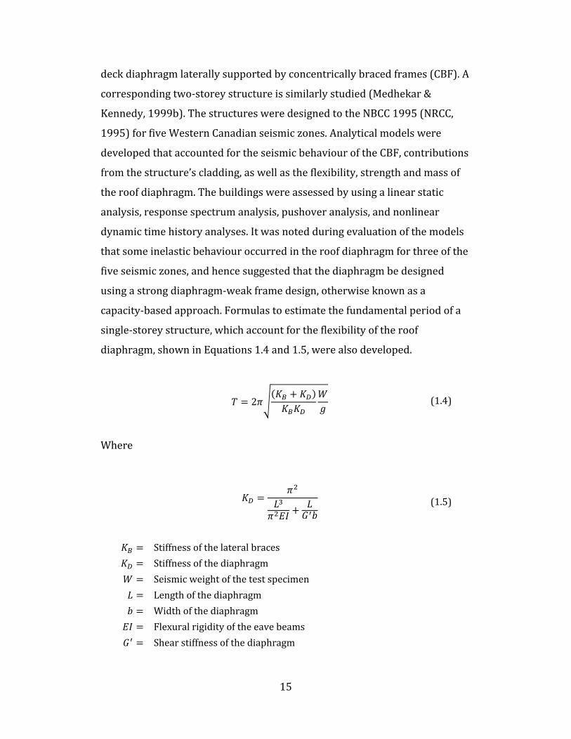
deck diaphragm laterally supported by concentrically braced frames (CBF). A corresponding two-storey structure is similarly studied (Medhekar & Kennedy, 1999b). The structures were designed to the NBCC 1995 (NRCC, 1995) for five Western Canadian seismic zones. Analytical models were developed that accounted for the seismic behaviour of the CBF, contributions from the structure’s cladding, as well as the flexibility, strength and mass of the roof diaphragm. The buildings were assessed by using a linear static analysis, response spectrum analysis, pushover analysis, and nonlinear dynamic time history analyses. It was noted during evaluation of the models that some inelastic behaviour occurred in the roof diaphragm for three of the five seismic zones, and hence suggested that the diaphragm be designed using a strong diaphragm-weak frame design, otherwise known as a capacity-based approach. Formulas to estimate the fundamental period of a single-storey structure, which account for the flexibility of the roof diaphragm, shown in Equations 1.4 and 1.5, were also developed. 2 (1.4) Where (1.5)

Stiffness of the lateral braces Stiffness of the diaphragm Seismic weight of the test specimen Length of the diaphragm Width of the diaphragm Flexural rigidity of the eave beams Shear stiffness of the diaphragm

16

Tremblay et al.: The study by Tremblay et al. (2008a) involved ambient vibration testing of a single-storey steel structure in Magog, Quebec, in order to measure the fundamental period of vibration in the two principal directions (Figure 1.3). A detailed 3D elastic model was then created in SAP2000 (CSI, 2010) in order to reproduce the results from field testing. The model consisted of properties and conditions that are typically adopted in structural design practice, and accounted for the spatial distribution of mass and stiffness to closely reproduce the conditions during ambient tests. All members were pinned at their ends, and the roof diaphragm was modelled using shell elements, to which were assigned an in-plane shear stiffness, G’, determined according to the SDI (Luttrell, 2004) procedure.

Figure 1.3 – 3D model and measured fundamental periods (Tremblay et al, 2008a) Periods computed in the two principal directions from the model as described (1.11 seconds, 1.00 seconds) were found to be approximately three times longer than those measured on site (0.39 seconds, 0.30 seconds). It was believed, however, that since the level of excitation in the field was very low, that bending moments in the member connections were not large enough to overcome the friction restraining rotation. Changes were thus made to the model by fixing the member ends, which caused the computed periods (0.79 seconds, 0.70 seconds) to be twice as large as those measured. Further modifications were made to the model by creating infinitely stiff braces and

17

walls, which led to shorter periods (0.74 seconds and 0.52 seconds). Recalculating the shear stiffness of the diaphragm assuming that friction prevented sliding of the diaphragm connections reduced the two fundamental periods of the model to 0.67 and 0.37 seconds, respectively. In the last version of the model, G’ was determined with the sheet length in the SDI calculations equal to the building’s dimensions to restrict warping deformations. This last change had the effect of decreasing the period of the model further to 0.34 seconds and 0.23 seconds, which better matched the test data. The results indicated that the effective lateral stiffness of a structure during ambient tests is considerably higher than assumed in design, however, during stronger ground motions, part of this apparent stiffness may not be present and the ambient periods are likely to be shorter than during an earthquake. 1.6.3.2 Laboratory and Field Studies

Tremblay, Berair and Filiatrault: Shake table testing on a 1:7.5 reduced scale building model with a flexible steel roof deck diaphragm was performed by Tremblay et al. (2000). Parameters under investigation included the stiffness of the roof diaphragm, ground motion characteristics, and in-plane mass, stiffness and strength eccentricities. It was determined from testing that the equation proposed by Medhekar and Kennedy (1997), which incorporates the flexibility of the roof diaphragm in the calculation of the fundamental period was valid. Additionally, the tests confirmed the findings from additional studies, namely that a dynamic amplification of the drift occurred from static levels on par with that observed by Tremblay and Stiemer (1996), and that the shear force demand was not linear and was also influenced by dynamic amplification.

18

Essa: Essa et al. (2001) performed monotonic and reversed cyclic tests on 19 diaphragm specimens in the structural engineering laboratory of École Polytechnique, in Montreal. The experimental setup consisted of a 6.1 m x 3.6 m cantilever frame with four overlain steel roof deck sheets, either 0.76 mm or 0.91 mm thick, connected in a 36/4 pattern with 305 mm sidelaps to form the diaphragm. Nine different combinations of deck-to-frame and deck-to-deck fasteners were considered in order to investigate the ability of the diaphragms to dissipate energy by deforming inelastically. It was determined that the inelastic behaviour, energy dissipation and ductility characteristics varied depending on the type of fasteners used. Additionally, the welded frame connections (without washers) showed limited amounts of ductility when compared with the other frame fastener types. It was recommended that button-punch sidelap connections be avoided when the diaphragm is detailed to perform inelastically due to their poor performance and questionable reliability. Martin: Two additional experimental studies were completed on 0.76 mm and 0.91 mm steel deck diaphragm specimens using the same test frame as Essa. The first study, under the responsibility of Martin (2002), involved an analytical component to determine the time history deformation demand response on roof diaphragms. Based on these results, two loading protocols were developed to mimic the expected inelastic behaviour, and were applied to 19 full-scale tests in the laboratory. It was determined that the response of the diaphragms was dominated by the connection behaviour. Preliminary values of the overstrength and ductility related R factors were proposed based on the frame and sidelap fasteners as follows: weld/button-punch (Rd = 1.0, Ro = 1.0), weld with washer/ weld with washer (Rd = 1.5, Ro = 1/φ), nail/weld with washer (Rd = 1.5, Ro = 1/φ), and nail/screw (Rd = 2.0, Ro = 1/φ).

19

Yang: The second study, completed by Yang (2003) featured an additional 12 tests that focused on the effect of non-structural components and end overlaps to the stiffness of the diaphragm. As well, diaphragm fasteners from two separate manufacturers, Hilti and ITW Buildex, were included in the scope of the study. The results obtained by Yang (2003) demonstrated that the non-structural roofing overlay impacted both the strength and stiffness of the specimens, with increases of 26% and 46% respectively. The effects of non-structural components were therefore found to not be negligible when 0.76 mm decks with a stiff gypsum board were investigated. When considering the impact of end overlaps, the single sheets of 6.1 m length used by Essa et al. (2001), and Martin (2002), were replaced by two sheets of roughly half the length of the originals to create the overlap condition. It was determined from the tests that the addition of the sheet end laps had little influence on the ultimate strength of the diaphragm, but did contribute to a significant decrease in shear stiffness. An average decrease of 35% was obtained when comparing the overlapped specimens to their respective single sheet counterparts due to the restriction of the warping deformations in the latter case. Finally, both mechanical fasteners provided similar shear resistances, however the ones manufactured by Hilti were on the order of 16% stiffer. Further information on the cantilever tests performed at École Polytechnique de Montréal can be found in Tremblay et al. (2003). Rogers and Tremblay: Rogers and Tremblay investigated the inelastic response of frame fasteners (2003a) as well as the behaviour of sidelap connections (2003b) for steel diaphragms under seismic loading. It was determined that with respect to frame fasteners, welds performed poorly by failing in a brittle manner.

20

Quality control of the welded tests was also a concern in the thinner specimens as the steel sheets were often not fastened to the entire perimeter of the weld, even in a controlled laboratory environment. Welds with washers failed in a more ductile mode due to bearing of the sheet steel on the weld metal, and connections of this type were more consistently reproduced. Nail and screw frame fasteners exhibited a pinched hysteretic behaviour and typically failed by bearing on the sheet steel and tilting of the fastener. Button-punch sidelaps were found to easily loosen during larger deformations, while welded sidelaps were effective at dissipating energy although their quality was once again a concern. Screwed sidelaps produced the most consistency in performance and were highly regarded from a constructability standpoint. Like their frame fastener equivalents, the sidelap screws exhibited a pinched hysteretic behaviour because of their tendency to tilt as the number of loading cycles increased. Further information with respect to connection tests can be found in the report by Rogers and Tremblay (2000). Lamarche: In-situ ambient vibration tests were performed on 22 buildings in Eastern and Western Canada and are covered in the work by Lamarche et al. (2004), Lamarche (2005) and Lamarche et al. (2009). The structures varied in size, roof mass, and spatial distribution of the lateral force resisting system, however each was constructed using steel roof deck diaphragms and supported laterally by steel braces. The purpose of this study was to obtain values for the fundamental period of the structures and compare them to the period calculation formulas listed in the NBCC 2005 (NRCC, 2005), which depend solely on the height of the structure. It was determined that the measured periods of the structures did not correspond well to the NBCC estimate. Rather, they were more closely correlated to the width of a structure, and to a parameter, Dneff, taken as the longest distance between two consecutive lateral load resisting systems. Regression models based on

21

these variables were proposed to more accurately predict the fundamental period of single-storey braced frames for low amplitude linear behaviour. 1.6.3.3 Large-Scale Diaphragm Experiments, Phases I and II Beginning in 2007, a series of dynamic tests were performed on ten different diaphragm specimens selected to replicate the most common configurations used in Canadian and US construction. These ten tests, covered in the work by Franquet (2010) and Franquet et al. (2010) consisted of Phases I and II of the large-scale dynamic diaphragm experiments, for which Phase III, covered in this thesis, subsequently followed. Information regarding the experimental frame setup can be found in Section 2.2. The test diaphragms consisted of 0.76 mm and 0.91 mm thick 38 x 914 mm corrugated steel deck profiles connected using various frame and sidelap fasteners as listed in Table 1.1. Each test was subjected to dynamic loading protocols in order to determine the change in stiffness with increased loading and to evaluate the seismic response of the diaphragm. One such protocol was then used to induce inelastic deformations in each specimen so that it could be repaired and retested allowing for the evaluation of the ductility of various diaphragm configurations. The diaphragm properties measured from the dynamic tests were compared with their respective strength and stiffness predictions determined using the SDI method (Luttrell, 2004), allowing for the comparison of the experimental values to commonly used design formulas. It was determined that with increasing excitation amplitude the fundamental period of the diaphragm elongates and that the shear stiffness lowers. This helps to explain why ambient vibration measurements taken from a building, such as done in the study performed by Lamarche et al. (2009), may not be representative of the behaviour of a structure during actual ground motions. When comparing the behaviour with the design predictions, it was determined that the SDI method can accurately predict the stiffness at ambient levels for fastener

22

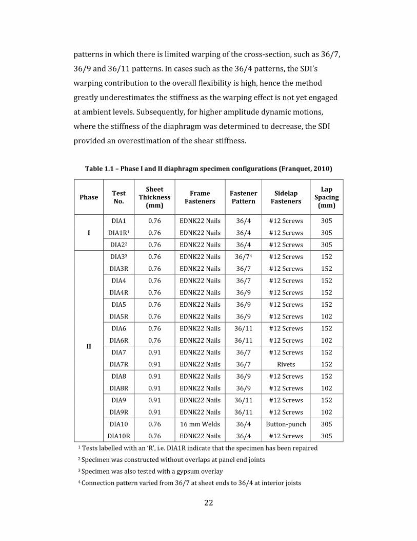
patterns in which there is limited warping of the cross-section, such as 36/7, 36/9 and 36/11 patterns. In cases such as the 36/4 patterns, the SDI’s warping contribution to the overall flexibility is high, hence the method greatly underestimates the stiffness as the warping effect is not yet engaged at ambient levels. Subsequently, for higher amplitude dynamic motions, where the stiffness of the diaphragm was determined to decrease, the SDI provided an overestimation of the shear stiffness. Table 1.1 – Phase I and II diaphragm specimen configurations (Franquet, 2010)

Phase Test No.

Sheet Thickness

(mm)

Frame Fasteners

Fastener Pattern

Sidelap Fasteners

Lap Spacing

(mm)

I

DIA1 0.76 EDNK22 Nails 36/4 #12 Screws 305 DIA1R1 0.76 EDNK22 Nails 36/4 #12 Screws 305 DIA22 0.76 EDNK22 Nails 36/4 #12 Screws 305

II

DIA33 0.76 EDNK22 Nails 36/74 #12 Screws 152 DIA3R 0.76 EDNK22 Nails 36/7 #12 Screws 152 DIA4 0.76 EDNK22 Nails 36/7 #12 Screws 152 DIA4R 0.76 EDNK22 Nails 36/9 #12 Screws 152 DIA5 0.76 EDNK22 Nails 36/9 #12 Screws 152 DIA5R 0.76 EDNK22 Nails 36/9 #12 Screws 102 DIA6 0.76 EDNK22 Nails 36/11 #12 Screws 152 DIA6R 0.76 EDNK22 Nails 36/11 #12 Screws 102 DIA7 0.91 EDNK22 Nails 36/7 #12 Screws 152 DIA7R 0.91 EDNK22 Nails 36/7 Rivets 152 DIA8 0.91 EDNK22 Nails 36/9 #12 Screws 152 DIA8R 0.91 EDNK22 Nails 36/9 #12 Screws 102 DIA9 0.91 EDNK22 Nails 36/11 #12 Screws 152 DIA9R 0.91 EDNK22 Nails 36/11 #12 Screws 102 DIA10 0.76 16 mm Welds 36/4 Button-punch 305 DIA10R 0.76 EDNK22 Nails 36/4 #12 Screws 305 1 Tests labelled with an ‘R’, i.e. DIA1R indicate that the specimen has been repaired 2 Specimen was constructed without overlaps at panel end joints 3 Specimen was also tested with a gypsum overlay 4 Connection pattern varied from 36/7 at sheet ends to 36/4 at interior joists

23

With regards to ultimate shear strength, all new specimens were able to attain a nominal strength greater than that predicted by the SDI. When considering repaired specimens only, approximately 50% were not able to achieve the predicted value likely due to residual damage from the initial inelastic test. Failure, in all cases, tended to concentrate at the outer thirds of the test setup and was generally more concentrated towards the end for the thicker specimens. Typical failure modes consisted of combinations of sheet distortion, nail bearing, nail failure, screw bearing, weld bearing, weld sheet tearing, and button-punch separation. Specimens connected using nails and screws exhibited a greater ability to dissipate energy than the welded counterpart. In the latter’s case, the peak load was sustained over multiple cycles, but the inelastic deformation capability, the difference in deformation between ultimate and yield levels, was minimal. 1.7 Summary There is a significant amount of previous research related to the study of steel roof deck diaphragms. Much of this information has been taken into consideration for the purpose of this project. For example, the strength and stiffness of all diaphragm specimens examined was calculated using the well-known SDI methodology (Luttrell, 2004). The selection of the specimens was heavily influenced by those chosen for Phases I and II of the project (Franquet, 2010), as they were selected to add to the thicknesses, fastener types and orientations previously studied. As well, the equation proposed by Medhekar and Kennedy (1997), which incorporates the shear stiffness of the diaphragm in the calculation of the fundamental period of vibration, was used as a comparison for results. Connection information has previously been gathered by Rogers and Tremblay (2003a, 2003b), however little information is known about the performance of the fasteners during tests in which the diaphragm has been repaired and re-tested after undergoing initial inelastic deformations. Should

24

the strength and stiffness properties be satisfactorily recuperated, it is feasible that such repair methods could be undertaken on actual buildings that have been damaged during an earthquake. Finally, many older single-storey structures in Canada have been constructed using welds and button-punches to connect the diaphragm; it has been shown by Essa (2001) and Martin (2002) that these fasteners may behave in a non-ductile manner when undergoing inelastic deformations. For these reasons, the inclusion of a retrofitted structure is also of significant interest.

25

Chapter 2 - LARGE-SCALE DYNAMIC DIAPHRAGM EXPERIMENTS

2.1 Test Overview As part of the large-scale steel roof deck diaphragm project, a total of 19 specimens involving various deck thicknesses, fastener types and spacing were tested in the structural engineering laboratory of École Polytechnique, in Montreal. The laboratory component of the project was divided into three phases: Phases I and II, which are covered in detail in the work by Franquet (2010), and Phase III, which fell under the responsibility of the author. A numerical modelling component of the diaphragm study is also underway. For the third phase of testing, nine diaphragm specimens were examined, with the goal being to evaluate the change in behaviour of the diaphragms under different levels and orientations of dynamic loading. The parameters of interest included the change in fundamental frequency and stiffness, the response to seismic loading, and the ductility demand and hysteretic behaviour under inelastic loading of the specimens. There was also a need to evaluate the diaphragm as a principal energy dissipating element. As such, the specimens were tested in both new and repaired states enabling information to be gained regarding various possible repair and retrofit scenarios. 2.2 Experimental Setup and Testing

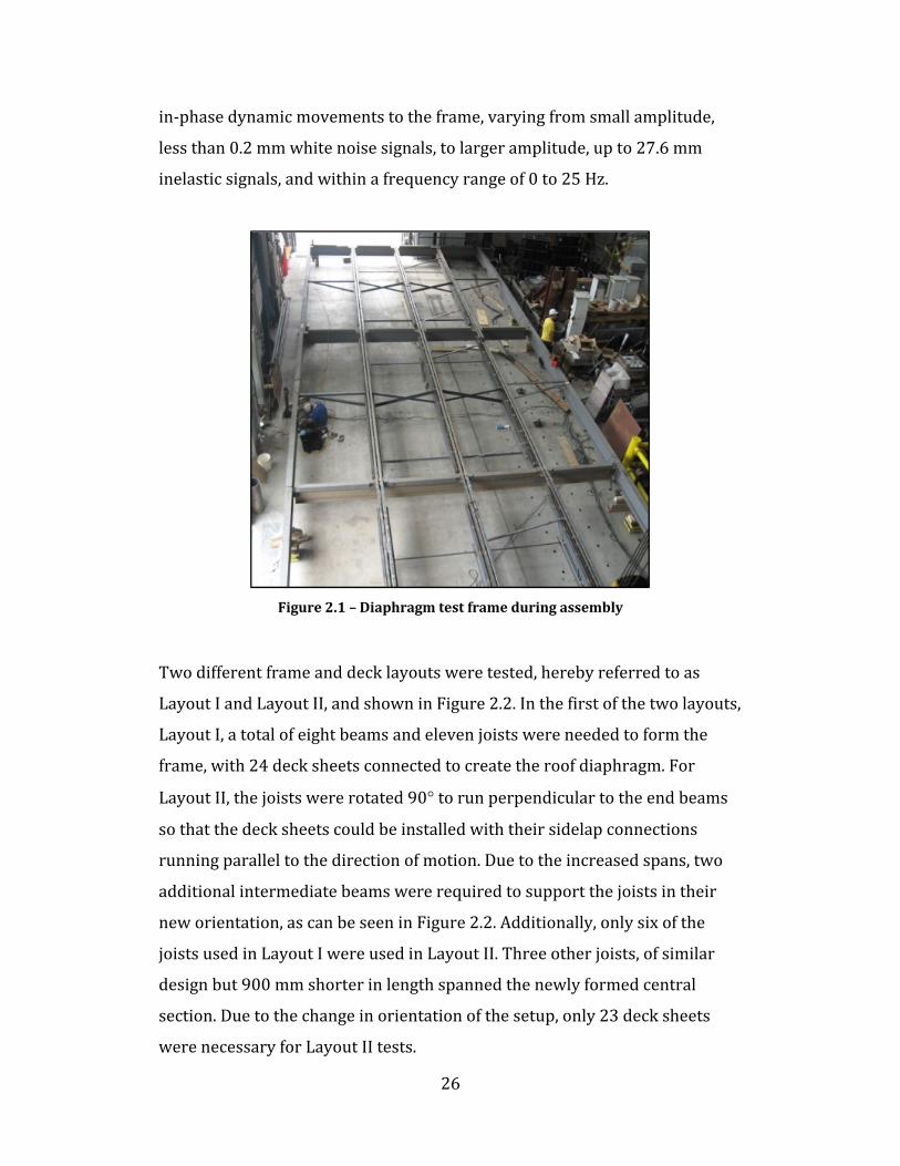
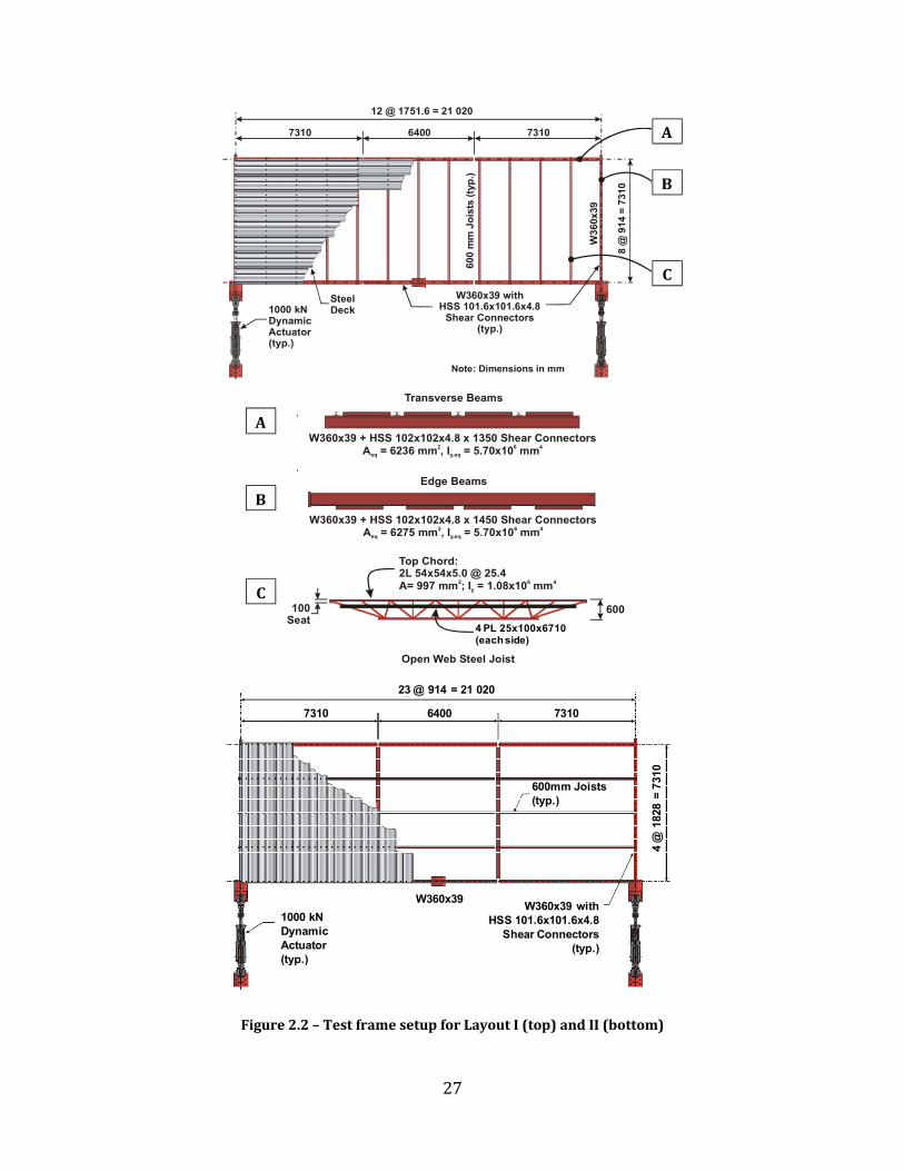
2.2.1 Test Frame The test frame, shown in Figure 2.1, was made of W-sections as well as open-web steel joists (OWSJ) in order to mimic the typical roof structure of a single-storey steel building. The entire 21.02 m wide by 7.31 m long structure was covered with steel decking to complete a typical test specimen. The frame was connected at each end to an MTS Series 244 high performance dynamic hydraulic actuator, with a force rating of 1000 kN and stroke length of 750 mm. The actuators were needed to induce the necessary in-plane and

26

in-phase dynamic movements to the frame, varying from small amplitude, less than 0.2 mm white noise signals, to larger amplitude, up to 27.6 mm inelastic signals, and within a frequency range of 0 to 25 Hz.

Figure 2.1 – Diaphragm test frame during assembly Two different frame and deck layouts were tested, hereby referred to as Layout I and Layout II, and shown in Figure 2.2. In the first of the two layouts, Layout I, a total of eight beams and eleven joists were needed to form the frame, with 24 deck sheets connected to create the roof diaphragm. For Layout II, the joists were rotated 90° to run perpendicular to the end beams so that the deck sheets could be installed with their sidelap connections running parallel to the direction of motion. Due to the increased spans, two additional intermediate beams were required to support the joists in their new orientation, as can be seen in Figure 2.2. Additionally, only six of the joists used in Layout I were used in Layout II. Three other joists, of similar design but 900 mm shorter in length spanned the newly formed central section. Due to the change in orientation of the setup, only 23 deck sheets were necessary for Layout II tests.

27

Figure 2.2 – Test frame setup for Layout I (top) and II (bottom)

7310

8 @

914

= 7

310

6400 7310

12 @ 1751.6 = 21 020

1000 kNDynamicActuator(typ.)

W360x39 withHSS 101.6x101.6x4.8

Shear Connectors(typ.)

Note: Dimensions in mm

W36

0x39

600

mm

Joi

sts

(typ.

)

SteelDeck

100Sea

C

B

A

PL 25x100x6710(each side)

Top Chord:2L 54x54x5.0 @ 25.4A= 997 mm ; I = 1.08x10 mm2 6 4

y

Open Web Steel Joist

600100Seat

W360x39 + HSS 102x102x4.8 x 1450 Shear ConnectorsA = 6275 mm , I = 5.70x10 mmeq y,

2 6 4eq

Edge Beams

W360x39 + HSS 102x102x4.8 x 1350 Shear ConnectorsA = 6236 mm , I = 5.70x10 mmeq y,

2 6 4eq

Transverse Beams

A

B

C

4 PL 25x100x6710(each side)

600mm Joists(typ.)

73107310 6400

23 @ 914 = 21 020

W360x391000 kNDynamicActuator(typ.)

W360x39 withHSS 101.6x101.6x4.8

Shear Connectors(typ.)

4 @

182

8 =

7310

28

2.2.1.1 Steel Beams The frame was assembled using 350W grade (Fy = 345 MPa, 50 ksi) W360x39 steel beams which formed the perimeter of the test area. Each beam had four evenly spaced HSS 102x102x4.8 sections with a length of either 1,350 mm or 1,450 mm welded to one flange, in order to create the mechanical connections through which shear was transferred from the frame to the diaphragm. In Layout I, the shear connectors on the transverse beams faced upwards and sat at the same elevation as the top flange of the edge beams as shown in Figure 2.3, which for this layout had their HSS segments facing downwards. Every beam was detailed so that it could be flipped upside down and used in both the Layout I and Layout II configurations; in Layout II the beams were rotated 180° so that the HSS sections of the edge beams faced upwards, running flush with the top flange of the transverse beams.

Figure 2.3 – Diaphragm connection to the beam flange and HSS shear connector

2.2.1.2 Open-web Steel Joists The joists used in the test setup were representative of those typically found in medium to long-span applications. Each joist measured 600 mm in depth and was designed to support a specified dead load of 2.12 kN/m and a

HSS shear connector Edge beam flange

29

specified live load of 3.80 kN/m over an assumed length of 12.0 m. In order to connect the joists to the underlying beams, a 100 mm long seat was used at both joist ends. The seats were then fixed to the beams by welding along the length of the seat. Once connected, the upper-chord of the joists ran level with the top of the HSS shear connectors which allowed for the deck sheets to be fastened to both frame components for testing. 2.2.1.3 Frame Supports In order to support the actuators, two reaction columns were installed on the strong-floor of the laboratory (Figure 2.4). These columns were fastened by using threaded rods that were post-tensioned using hydraulic pressure in order to ensure that no slipping of the base would occur during testing. The base ends of the actuators were then attached to the columns by fastening them through their end swivels using four 38.1 mm (1-1/2”) threaded connector studs to a 51 mm (2”) thick steel plate. This plate was itself attached to the reaction column using 28.6 mm (1-1/8”) diameter bolts. All bolts used in the attachments were installed to meet specified torque levels to minimize possible detachments of the connected parts during the tests.

Figure 2.4 – Actuator (black) installed on reaction column (burgundy)

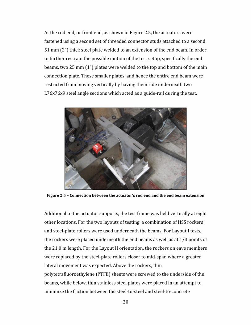
30

At the rod end, or front end, as shown in Figure 2.5, the actuators were fastened using a second set of threaded connector studs attached to a second 51 mm (2”) thick steel plate welded to an extension of the end beam. In order to further restrain the possible motion of the test setup, specifically the end beams, two 25 mm (1”) plates were welded to the top and bottom of the main connection plate. These smaller plates, and hence the entire end beam were restricted from moving vertically by having them ride underneath two L76x76x9 steel angle sections which acted as a guide-rail during the test.

Figure 2.5 – Connection between the actuator’s rod end and the end beam extension Additional to the actuator supports, the test frame was held vertically at eight other locations. For the two layouts of testing, a combination of HSS rockers and steel-plate rollers were used underneath the beams. For Layout I tests, the rockers were placed underneath the end beams as well as at 1/3 points of the 21.0 m length. For the Layout II orientation, the rockers on eave members were replaced by the steel-plate rollers closer to mid-span where a greater lateral movement was expected. Above the rockers, thin polytetrafluoroethylene (PTFE) sheets were screwed to the underside of the beams, while below, thin stainless steel plates were placed in an attempt to minimize the friction between the steel-to-steel and steel-to-concrete

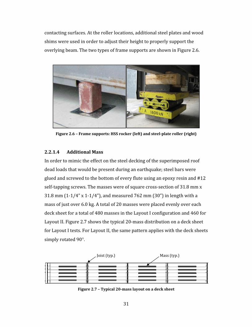
31

contacting surfaces. At the roller locations, additional steel plates and wood shims were used in order to adjust their height to properly support the overlying beam. The two types of frame supports are shown in Figure 2.6.

Figure 2.6 – Frame supports: HSS rocker (left) and steel-plate roller (right)

2.2.1.4 Additional Mass In order to mimic the effect on the steel decking of the superimposed roof dead loads that would be present during an earthquake; steel bars were glued and screwed to the bottom of every flute using an epoxy resin and #12 self-tapping screws. The masses were of square cross-section of 31.8 mm x 31.8 mm (1-1/4” x 1-1/4”), and measured 762 mm (30”) in length with a mass of just over 6.0 kg. A total of 20 masses were placed evenly over each deck sheet for a total of 480 masses in the Layout I configuration and 460 for Layout II. Figure 2.7 shows the typical 20-mass distribution on a deck sheet for Layout I tests. For Layout II, the same pattern applies with the deck sheets simply rotated 90°.

Figure 2.7 – Typical 20-mass layout on a deck sheet

Joist (typ.) Mass (typ.)

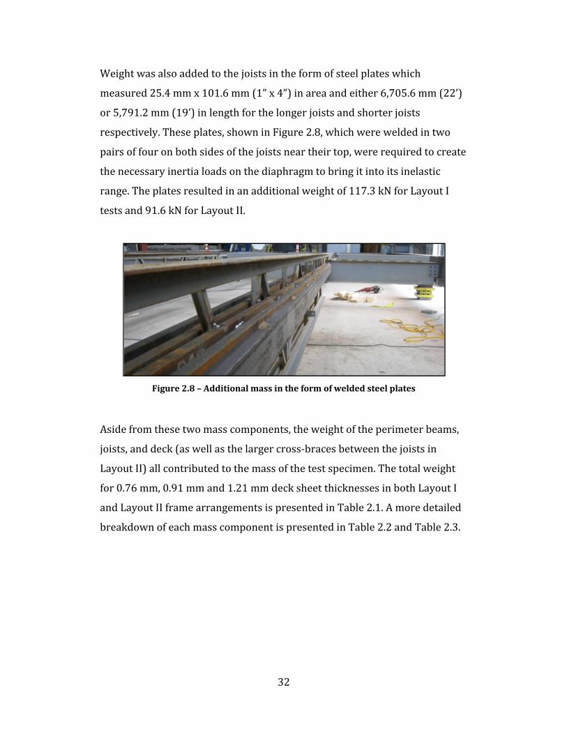
32

Weight was also added to the joists in the form of steel plates which measured 25.4 mm x 101.6 mm (1” x 4”) in area and either 6,705.6 mm (22’) or 5,791.2 mm (19’) in length for the longer joists and shorter joists respectively. These plates, shown in Figure 2.8, which were welded in two pairs of four on both sides of the joists near their top, were required to create the necessary inertia loads on the diaphragm to bring it into its inelastic range. The plates resulted in an additional weight of 117.3 kN for Layout I tests and 91.6 kN for Layout II.

Figure 2.8 – Additional mass in the form of welded steel plates Aside from these two mass components, the weight of the perimeter beams, joists, and deck (as well as the larger cross-braces between the joists in Layout II) all contributed to the mass of the test specimen. The total weight for 0.76 mm, 0.91 mm and 1.21 mm deck sheet thicknesses in both Layout I and Layout II frame arrangements is presented in Table 2.1. A more detailed breakdown of each mass component is presented in Table 2.2 and Table 2.3.

33

Table 2.1 – Total weight of test setup

Thickness (mm)

Weight (kN)

Layout I Layout II 0.76 202.5 182.7 0.91 205.0 185.1 1.21 209.9 190.0 Table 2.2 – Weight of individual components (Layout I)

Component Weight

(kN)

Thickness 0.76 0.91 1.21 Steel Deck 13.2 15.6 20.6 Steel Bars 28.4 Steel Plates 117.3 Joists 13.7 Transverse Eave Beams 20.2 End Beams 9.7 Total 202.5 205.0 209.9

Table 2.3 – Weight of individual components (Layout II)

Component Weight (kN)

Thickness 0.76 0.91 1.21 Steel Deck 12.9 15.3 20.2 Steel Bars 27.2 Steel Plates 91.6 Joists 10.8 Transverse Eave Beams 20.2 End Beams 9.7 Intermediate Beams 7.0 Additional Cross-Bracing 3.3 Total 182.7 185.1 190.0

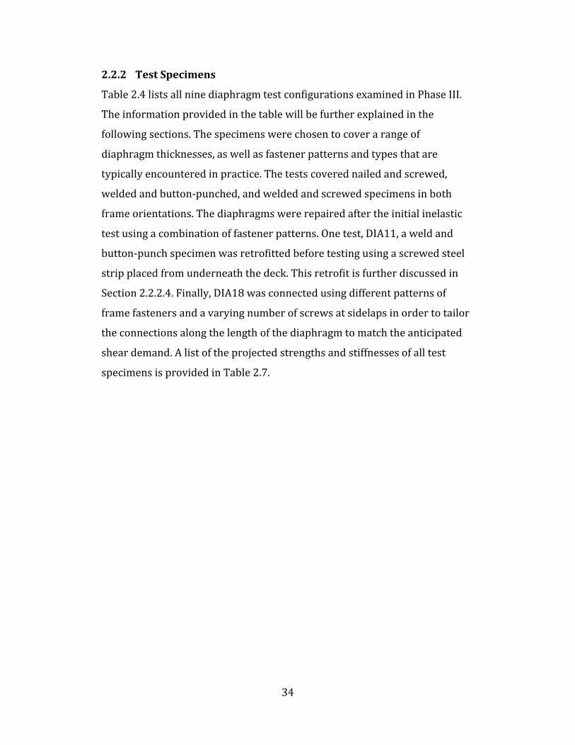
34

2.2.2 Test Specimens Table 2.4 lists all nine diaphragm test configurations examined in Phase III. The information provided in the table will be further explained in the following sections. The specimens were chosen to cover a range of diaphragm thicknesses, as well as fastener patterns and types that are typically encountered in practice. The tests covered nailed and screwed, welded and button-punched, and welded and screwed specimens in both frame orientations. The diaphragms were repaired after the initial inelastic test using a combination of fastener patterns. One test, DIA11, a weld and button-punch specimen was retrofitted before testing using a screwed steel strip placed from underneath the deck. This retrofit is further discussed in Section 2.2.2.4. Finally, DIA18 was connected using different patterns of frame fasteners and a varying number of screws at sidelaps in order to tailor the connections along the length of the diaphragm to match the anticipated shear demand. A list of the projected strengths and stiffnesses of all test specimens is provided in Table 2.7.

35

Table 2.4 – Phase III diaphragm test specimen configurations

Layout Test No. Deck

Profile

Sheet Thickness

(mm)

Frame Fasteners

Fastener Pattern

End Overlap

Sidelap Fasteners

Lap Spacing

(mm)

I

DIA11 38x914 0.76 16 mm Welds 36/4 36/7 Button-punch 305 DIA12 38x914 1.21 EDNK22 Nails 36/7 36/7 #12 Screws 152 DIA12R1 EDNK22 Nails 36/7 36/7 #12 Screws 152 DIA13 38x914 1.21 19 mm welds 36/7 36/7 #12 Screws 152 DIA13R EDNK22 Nails 36/7 36/7 #12 Screws 152 DIA14 38x914 1.21 EDNK22 Nails 36/9 36/9 #12 Screws 102

II

DIA15 38x914 0.76 16 mm Welds 36/4 N/A Button-punch 305 DIA15R EDNK22 Nails 36/4 N/A #12 Screws 305 DIA16 38x914 0.76 EDNK22 Nails 36/7 N/A #12 Screws 152 DIA16R EDNK22 Nails 36/9 N/A #12 Screws 152 DIA17 38x914 0.91 EDNK22 Nails 36/7 N/A #12 Screws 152 DIA17R EDNK22 Nails 36/9 N/A #12 Screws 152 DIA18 38x914 0.91 EDNK22 Nails Tailored N/A #12 Screws Tailored DIA18R EDNK22 Nails 36/7 N/A #12 Screws 102 DIA19 38x914 1.21 19 mm Welds 36/7 N/A #12 Screws 152 DIA19R EDNK22 Nails 36/7 N/A #12 Screws 152 1 All tests labelled with an ‘R’, i.e. DIA12R indicates that the original specimen has been repaired.

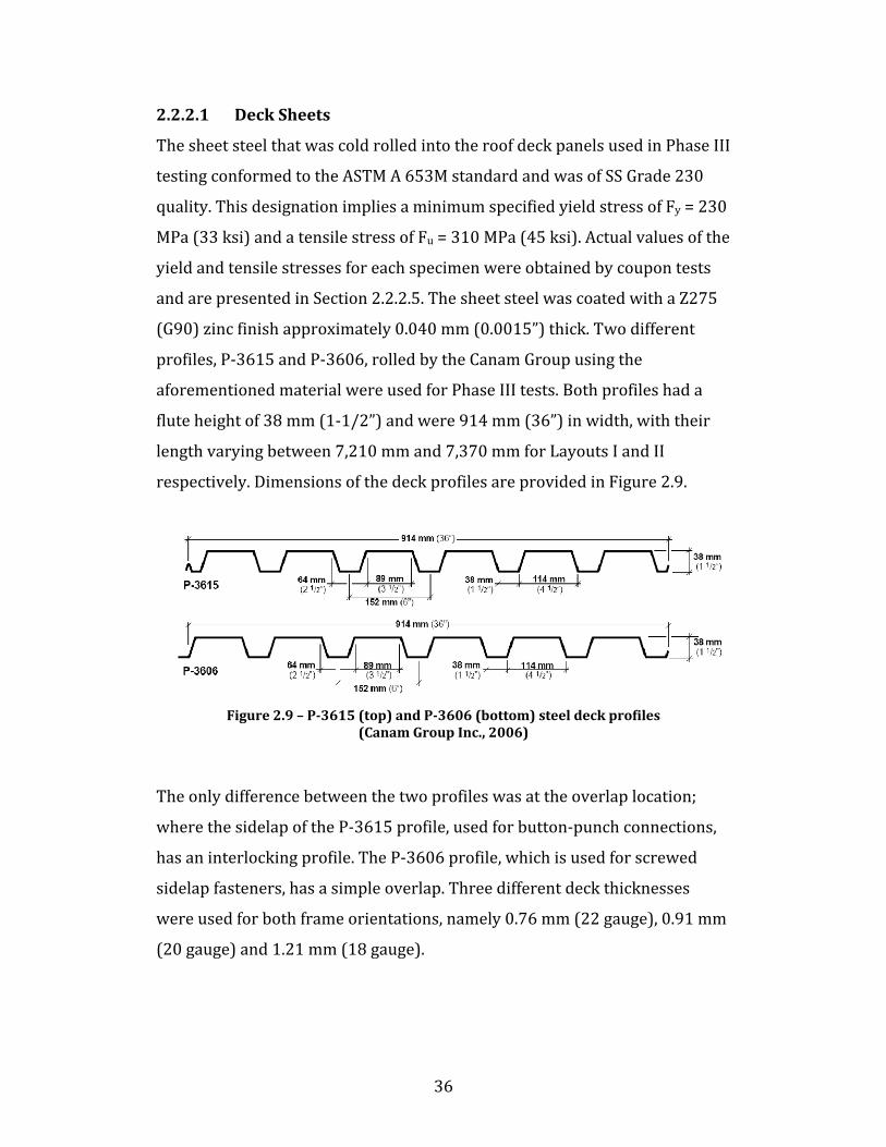
36

2.2.2.1 Deck Sheets The sheet steel that was cold rolled into the roof deck panels used in Phase III testing conformed to the ASTM A 653M standard and was of SS Grade 230 quality. This designation implies a minimum specified yield stress of Fy = 230 MPa (33 ksi) and a tensile stress of Fu = 310 MPa (45 ksi). Actual values of the yield and tensile stresses for each specimen were obtained by coupon tests and are presented in Section 2.2.2.5. The sheet steel was coated with a Z275 (G90) zinc finish approximately 0.040 mm (0.0015”) thick. Two different profiles, P-3615 and P-3606, rolled by the Canam Group using the aforementioned material were used for Phase III tests. Both profiles had a flute height of 38 mm (1-1/2”) and were 914 mm (36”) in width, with their length varying between 7,210 mm and 7,370 mm for Layouts I and II respectively. Dimensions of the deck profiles are provided in Figure 2.9.

Figure 2.9 – P-3615 (top) and P-3606 (bottom) steel deck profiles

(Canam Group Inc., 2006) The only difference between the two profiles was at the overlap location; where the sidelap of the P-3615 profile, used for button-punch connections, has an interlocking profile. The P-3606 profile, which is used for screwed sidelap fasteners, has a simple overlap. Three different deck thicknesses were used for both frame orientations, namely 0.76 mm (22 gauge), 0.91 mm (20 gauge) and 1.21 mm (18 gauge).

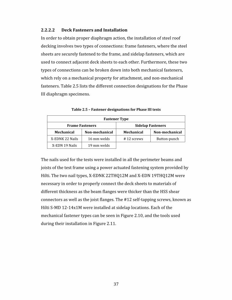
37

2.2.2.2 Deck Fasteners and Installation In order to obtain proper diaphragm action, the installation of steel roof decking involves two types of connections: frame fasteners, where the steel sheets are securely fastened to the frame, and sidelap fasteners, which are used to connect adjacent deck sheets to each other. Furthermore, these two types of connections can be broken down into both mechanical fasteners, which rely on a mechanical property for attachment, and non-mechanical fasteners. Table 2.5 lists the different connection designations for the Phase III diaphragm specimens. Table 2.5 – Fastener designations for Phase III tests

Fastener Type Frame Fasteners Sidelap Fasteners

Mechanical Non-mechanical Mechanical Non-mechanical X-EDNK 22 Nails 16 mm welds # 12 screws Button-punch X-EDN 19 Nails 19 mm welds The nails used for the tests were installed in all the perimeter beams and joists of the test frame using a power actuated fastening system provided by Hilti. The two nail types, X-EDNK 22THQ12M and X-EDN 19THQ12M were necessary in order to properly connect the deck sheets to materials of different thickness as the beam flanges were thicker than the HSS shear connectors as well as the joist flanges. The #12 self-tapping screws, known as Hilti S-MD 12-14x1M were installed at sidelap locations. Each of the mechanical fastener types can be seen in Figure 2.10, and the tools used during their installation in Figure 2.11.

38

Figure 2.10 – Mechanical fasteners before and after installation

Figure 2.11 – Power-actuated fastening tool for nails (left) and screwdriver with

stand-up handles (right)

39

Phase III of the testing program involved four welded specimens; two of which, DIA11 and DIA15 were connected using 16 mm arc-spot welds and button-punch sidelaps, and two others, DIA13 and DIA19 with 19 mm arc-spot welds with screws at the sheet-to-sheet connections. In all cases, the welds were made by a certified welder using 1/8” E6011 (E4311) electrodes. Two different welders were used which explains the differences in the time to weld each specimen. DIA11 and DIA13 were done by one individual, while work on DIA15 and DIA19 was done by another. Table 2.6 contains a summary of information for each of the four welded specimens. Table 2.6 – Total and average values for Phase III welded specimens

Test Total

Number of Welds

Weld Diameter for Calculations

(mm)

Average Weld Diameter

(mm)

Time to Weld Specimen

(min) DIA11 536 16.0 16.2 601 DIA13 901 19.0 17.4 1601 DIA15 580 16.0 15.3 210 DIA19 871 19.0 17.5 255 1The differences in weld times are because a different welder worked on specimens DIA11 and DIA13 The button-punch connections were installed using a crimping tool that creates an indent between two overlapped deck sheets in order to prevent slippage and provide shear resistance. Figure 2.12 displays the typical non-mechanical fasteners used in DIA11, DIA13, DIA15 and DIA19 Phase III tests.

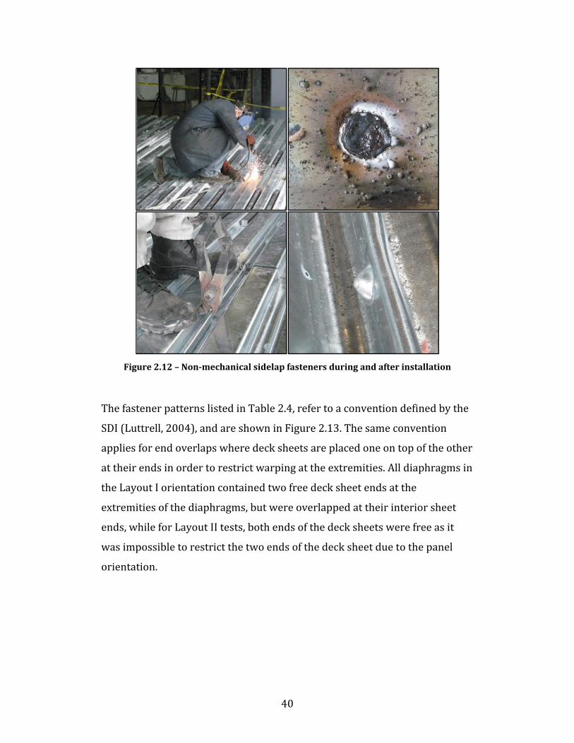
40

Figure 2.12 – Non-mechanical sidelap fasteners during and after installation The fastener patterns listed in Table 2.4, refer to a convention defined by the SDI (Luttrell, 2004), and are shown in Figure 2.13. The same convention applies for end overlaps where deck sheets are placed one on top of the other at their ends in order to restrict warping at the extremities. All diaphragms in the Layout I orientation contained two free deck sheet ends at the extremities of the diaphragms, but were overlapped at their interior sheet ends, while for Layout II tests, both ends of the deck sheets were free as it was impossible to restrict the two ends of the deck sheet due to the panel orientation.

41

Figure 2.13 – Fastener pattern configurations (Canam Group Inc., 2007) The SDI diaphragm design method was used to calculate the in-plane strength and stiffness of each test specimen. Using this method, the shear strength of the diaphragm, Sn, is limited by the lesser of the following four factors: the outer edge panel resistance, the interior panel resistance, the resistance of the corner fastener, and the overall shear buckling of the diaphragm. Typically, the overall shear buckling failure mode of a diaphragm is only a concern for shallow decks that have closely spaced connections, and although this mode governed the resistance of some specimens, such as DIA14, DIA16/16R, DIA17R and DIA18/18R, this failure mode was ignored because previous testing in Phases I and II had shown it not to control. The stiffness value, G’, is calculated by taking into account the flexibility of the steel, the flexibility due to warping of the cross section, and the flexibility of the connections. Table 2.7 lists both the shear strength and stiffness values for each of the Phase III specimens. Two cases have been included in the table because the strength and stiffness characteristics of every specimen were calculated in two ways: Case A, which considers each sheet to act as an independent panel with a length of 7,000 mm, and Case B, which considers the full 21,000 mm length acting as one panel due to the assumption that the panel end overlaps restrict warping of the deck at the interior of the

42

diaphragm test specimen. Because of the absence of end overlaps in Layout II, Case B values are not applicable. Table 2.7 – Phase III SDI method strength and stiffness predictions

Specimen

Case A Case B

Nominal Shear

Resistance, Sn (kN/m)

Rigidity, G’ (kN/mm)

Nominal Shear

Resistance, Sn (kN/m)

Rigidity, G’ (kN/mm)

DIA11 24.81 16.32 22.21 22.82 DIA12 38.6 31.1 37.5 37.8 DIA12R 38.6 31.1 37.5 37.8 DIA13 44.7 31.3 43.0 38.1 DIA13R 38.6 31.1 37.5 37.8 DIA14 55.7 34.8 54.2 43.6 DIA15 8.13 3.61 --- --- DIA15R 12.6 4.33 --- --- DIA16 23.6 17.1 --- --- DIA16R 28.2 17.5 --- --- DIA17 28.2 21.9 --- --- DIA17R 33.7 22.5 --- --- DIA183 42.0 23.6 --- --- DIA18R 34.8 23.6 --- --- DIA19 43.1 31.1 --- --- DIA19R 37.3 30.9 --- --- 1Resistance calculated assuming the frame fasteners and sidelap fasteners work in parallel (Eq. 2.1) 2Rigidity calculated assuming the frame fasteners and sidelap fasteners work in parallel (Eq. 2.2) 3Resistance and rigidity listed is that of the end panel Every specimen’s strength and stiffness were calculated using the properties of the individual frame and sidelap fasteners, except for the retrofit, DIA11, which had different connector types acting together in an undamaged state. For such a scenario, it was assumed that the nail and weld frame fasteners, as

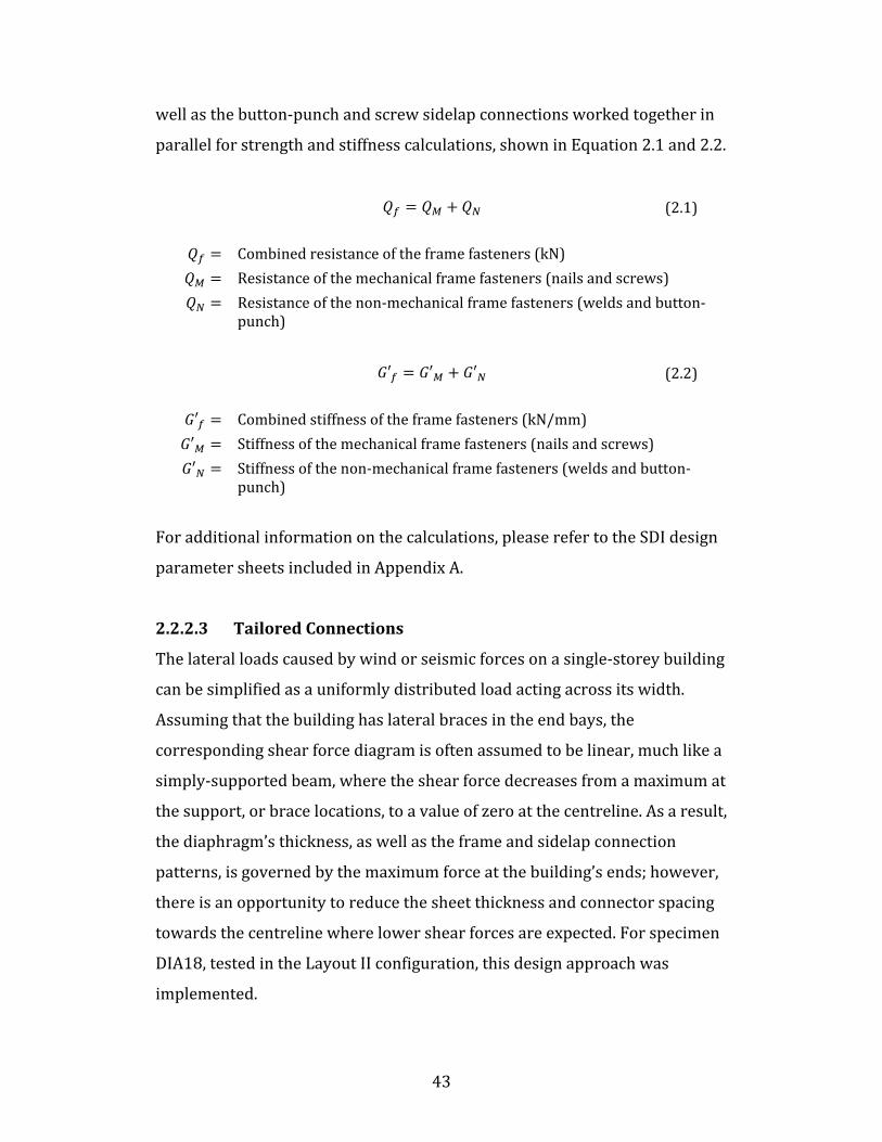
43

well as the button-punch and screw sidelap connections worked together in parallel for strength and stiffness calculations, shown in Equation 2.1 and 2.2. (2.1) Combined resistance of the frame fasteners (kN) Resistance of the mechanical frame fasteners (nails and screws) Resistance of the non-mechanical frame fasteners (welds and button-punch) (2.2) Combined stiffness of the frame fasteners (kN/mm) Stiffness of the mechanical frame fasteners (nails and screws) Stiffness of the non-mechanical frame fasteners (welds and button-punch) For additional information on the calculations, please refer to the SDI design parameter sheets included in Appendix A. 2.2.2.3 Tailored Connections The lateral loads caused by wind or seismic forces on a single-storey building can be simplified as a uniformly distributed load acting across its width. Assuming that the building has lateral braces in the end bays, the corresponding shear force diagram is often assumed to be linear, much like a simply-supported beam, where the shear force decreases from a maximum at the support, or brace locations, to a value of zero at the centreline. As a result, the diaphragm’s thickness, as well as the frame and sidelap connection patterns, is governed by the maximum force at the building’s ends; however, there is an opportunity to reduce the sheet thickness and connector spacing towards the centreline where lower shear forces are expected. For specimen DIA18, tested in the Layout II configuration, this design approach was implemented.

44

In order to tailor the connections to the anticipated shear demand of the specimen, it was decided, because of the limited size of the test frame, to reduce the fastener spacing towards the centreline and keep the thickness of the deck sheets constant. As listed in Table 2.4, a deck having a thickness of 0.91 mm and connected with nails and screws was chosen. The next step was to set a required design shear for the resistance of the outermost panel. To allow for comparison to similar Layout II specimens, such as DIA17, a value of 42.0 kN/m was selected. By reducing this number to match a resistance of 0 kN/m at the diaphragm’s centreline, the fastener spacing was then reduced to best match the shear resistance of a sheet with the shear force expected to develop at a particular location along the length. This shear resistance was determined assuming an interior panel failure mode from the SDI strength predictions, which was based on observations from previous Layout II tests. The patterns adopted for sheets 11 and 12 incorporate the fewest nail and sidelap fasteners to provide as low a resistance as possible. Table 2.8 lists the fastener patterns as well as the shear resistance calculated using the SDI method that were used over half the test specimen. The same pattern was repeated symmetrically over the remaining deck sheets. A schematic illustrating how the fastener pattern varied over the length of the diaphragm is provided in Figure 2.14. At the locations of the end beams and intermediate beams, nails, as opposed to screws were used to connect adjacent deck sheets at sidelaps. The first row of numbers (shown in red) represents the frame fastener pattern of each sheet, while the second row gives the total number of sidelap fasteners.

45

Table 2.8 – Frame fastener patterns and average strengths for DIA18

Sheet No.

Frame Fastener Pattern

Sidelap Fasteners per Panel

Actual Shear

Resistance, Sn

(kN/m)

Target Shear

Resistance, Sn

(kN/m)

Provided/ Target

Left Edge Right Edge 1 36/7 64 64 42.0 42.0 1.00 2 36/7 64 48 37.7 38.2 0.99 3 36/7 48 44 32.4 34.4 0.94 4 36/7 44 36 29.3 30.5 0.96 5 36/7 36 32 26.1 26.7 0.98 6 36/7 32 24 22.9 22.9 1.00 7 36/7 24 20 19.7 19.1 1.03 8 36/7 20 20 16.2 15.3 1.06 9 36/4 20 8 13.0 11.5 1.13 10 36/4 8 4 8.8 7.6 1.16 11 36/4 4 4 7.8 3.8 2.05 12 36/4 4 4 7.8 0.0 N/A

46

46

Figure 2.14 – Tailored fastener pattern for DIA18

CL

47

2.2.2.4 Connection Repairs Every diaphragm specimen was tested in two different states: new and repaired. Test DIA11 was the exception as it was tested only once in the new state after having been retrofitted. For the other specimens, many of the connectors showed signs of damage after the initial inelastic test as described in Section 2.5.5.1. In an attempt to recover the diaphragm’s original shear stiffness and strength, these connections were repaired by installing an adjacent fastener. This second set of testing allowed for the evaluation of the feasibility of particular repair and retrofit schemes. Table 2.9 describes the repair methods used for each of the diaphragm specimens. Repair procedures followed similar guidelines for both frame fasteners and sidelap fasteners. In the case of damaged nails, the connector was left in place and another nail was installed at a short distance from the damaged one or at a location where the sheet was undamaged. For specimens that were fastened using welds, two different procedures were used. For the welded and button-punched specimens, a nail was installed at all weld locations whether or not the connector displayed signs of damage, while for specimens that were welded to the frame and screwed at sidelaps, nails were installed nearby the damaged weld locations in a symmetric pattern on both sides of the diaphragm mid-span, i.e., for both the north and south sides of the diaphragm. Finally, for all screwed sidelaps, where the connection showed signs of tilting or bearing damage, the screw was first removed and then replaced by a new one adjacent to the original damaged location. Typical examples of repaired connections are given in Figure 2.15.

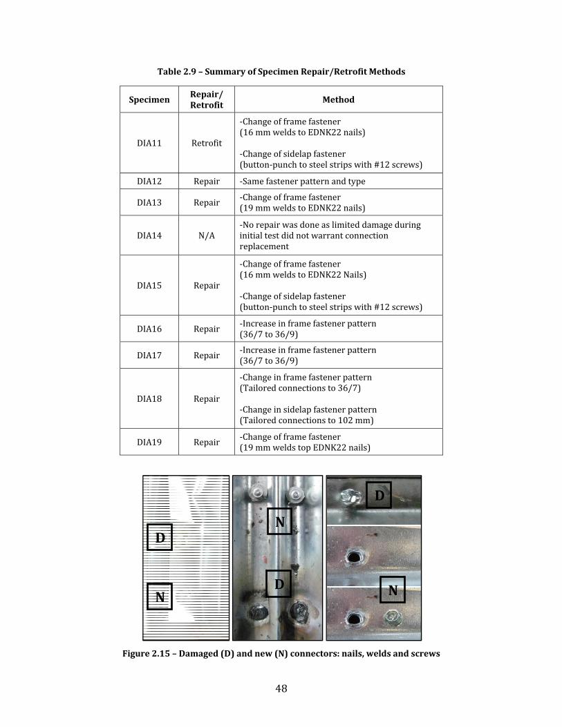
48

Table 2.9 – Summary of Specimen Repair/Retrofit Methods

Specimen Repair/ Retrofit

Method

DIA11 Retrofit -Change of frame fastener (16 mm welds to EDNK22 nails) -Change of sidelap fastener (button-punch to steel strips with #12 screws) DIA12 Repair -Same fastener pattern and type DIA13 Repair -Change of frame fastener (19 mm welds to EDNK22 nails) DIA14 N/A -No repair was done as limited damage during initial test did not warrant connection replacement DIA15 Repair -Change of frame fastener (16 mm welds to EDNK22 Nails) -Change of sidelap fastener (button-punch to steel strips with #12 screws) DIA16 Repair -Increase in frame fastener pattern (36/7 to 36/9) DIA17 Repair -Increase in frame fastener pattern (36/7 to 36/9) DIA18 Repair -Change in frame fastener pattern (Tailored connections to 36/7) -Change in sidelap fastener pattern (Tailored connections to 102 mm) DIA19 Repair -Change of frame fastener (19 mm welds top EDNK22 nails)

Figure 2.15 – Damaged (D) and new (N) connectors: nails, welds and screws

N

N

N

D

D

D

49

For the two tests that were connected at their sidelaps with button-punches, adjacent interlocking deck sheets were repaired (or retrofitted) using screwed steel strips from underneath the test frame. These Grade 230 steel strips, which measured 1.21 mm thick, 50 mm wide and 1,215 mm long were fastened from underneath using typical #12 self-tapping screw sidelap fasteners. Five such screws were spaced between joists at an interval of 305 mm (12”) along one side of the interlock, with the same pattern being repeated in a second row to ensure that the plate was connected to both deck sheets. Figure 2.16, taken from underneath the frame shows the final installation and a schematic of a typical screwed steel strip repair.

Figure 2.16 – Screwed steel strip repair of button-punched connections 2.2.2.5 Material Properties Coupons were cut and tests carried out to determine the base metal thickness and mechanical properties of the steel deck. A single set of tests was performed for diaphragms of the same thickness that originated from the same coil. In all, three samples were tested for each diaphragm according to ASTM A370 (2006) requirements, with average values being presented in Table 2.10. A crosshead rate in the elastic range of the material of 0.6

50

mm/min was used, with the speed being increased to 6 mm/min after yielding. An extensometer with a 50 mm gauge length was used to measure the elongation of the coupons. During one of the three tests for a diaphragm specimen, the crosshead movement was paused at three occasions, once in the elastic range and twice in the inelastic in order to obtain the static values of yield and ultimate stresses. Once the coupon tests were completed, a 10% hydrochloric acid solution was used to remove the zinc coating from the surface of the material in order to measure the true thickness of the base metal. Table 2.10 – Summary of material properties

Specimen Nominal

Thickness (mm)

Base Metal Thickness

(mm)

Yield Stress, Fy

(MPa)

Ultimate Stress, Fu

(MPa) Fu/Fy

Elongation (%) DIA111 0.76 --- --- --- --- --- DIA12 1.21 1.21 280 342 1.22 37.0 DIA13 1.21 1.22 299 349 1.17 37.6 DIA14 1.21 1.22 286 345 1.21 35.8 DIA15 0.76 0.77 315 362 1.15 37.9 DIA16 0.76 0.76 303 350 1.16 35.8 DIA17 0.91 0.91 284 364 1.28 30.2 DIA18 0.91 0.91 286 366 1.28 28.2 DIA19 1.21 1.21 291 344 1.18 36.0 1No coupons were taken for DIA11 As can be seen, the base metal thickness values were either larger than or equal to the nominal thickness. As well, the yield stress and ultimate stress values measure significantly above the 230 MPa and 310 MPa values used for design. The relationship between Fu/Fy was in all instances greater than 1.08, the minimum ratio required by CSA S136 (2007) and the measured elongation over a gauge length of 50 mm also satisfies the 10% minimum.

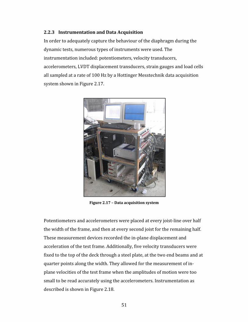
51

2.2.3 Instrumentation and Data Acquisition In order to adequately capture the behaviour of the diaphragm during the dynamic tests, numerous types of instruments were used. The instrumentation included: potentiometers, velocity transducers, accelerometers, LVDT displacement transducers, strain gauges and load cells all sampled at a rate of 100 Hz by a Hottinger Messtechnik data acquisition system shown in Figure 2.17.

Figure 2.17 – Data acquisition system Potentiometers and accelerometers were placed at every joist-line over half the width of the frame, and then at every second joist for the remaining half. These measurement devices recorded the in-plane displacement and acceleration of the test frame. Additionally, five velocity transducers were fixed to the top of the deck through a steel plate, at the two end beams and at quarter points along the width. They allowed for the measurement of in-plane velocities of the test frame when the amplitudes of motion were too small to be read accurately using the accelerometers. Instrumentation as described is shown in Figure 2.18.

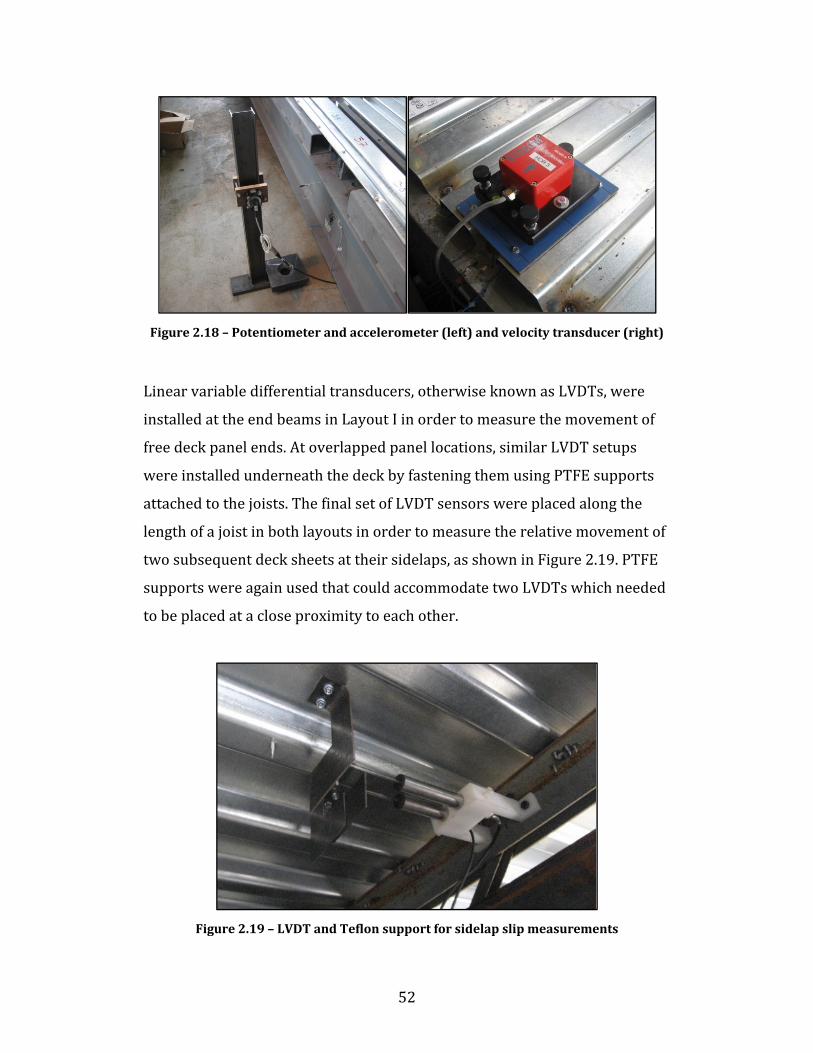
52

Figure 2.18 – Potentiometer and accelerometer (left) and velocity transducer (right) Linear variable differential transducers, otherwise known as LVDTs, were installed at the end beams in Layout I in order to measure the movement of free deck panel ends. At overlapped panel locations, similar LVDT setups were installed underneath the deck by fastening them using PTFE supports attached to the joists. The final set of LVDT sensors were placed along the length of a joist in both layouts in order to measure the relative movement of two subsequent deck sheets at their sidelaps, as shown in Figure 2.19. PTFE supports were again used that could accommodate two LVDTs which needed to be placed at a close proximity to each other.

Figure 2.19 – LVDT and Teflon support for sidelap slip measurements

53

Finally, strain gauges were attached to the inner and outer webs of the eave beams at their mid-height. These were placed so as to record the axial deformations of the W360x39 sections which could subsequently be converted into stress levels used for modelling purposes. Layouts and locations of all the instrumentation can be found in Figure 2.20.

Potentiometers and accelerometers measuring in the direction of the arrow Velocity transducers LVDT’s measuring the relative slip at sidelap connections LVDT’s measuring the longitudinal displacement at panel ends Strain gauges on the web of the eave beams

Figure 2.20 – Instrumentation setup for Layout I (top) and II (bottom) tests

54

The differences in instrumentation between the Layout I and II tests was that all the LVDTs fastened to the joists which measured the relative slip at sidelap locations were rotated 90° with the joists. The inner LVDTs from Layout I that measured longitudinal displacement at sheet ends were no longer needed in Layout II since there were no end overlaps in the new orientation. The potentiometers, accelerometers and velocity transducers were only slightly shifted from their Layout I locations in order to line up with the new deck sheet sidelap lines, while the strain gauges remained in the same locations. 2.2.4 Experimental Loading Protocols Each of the diaphragm specimens, both new and repaired were tested under four dynamic loading protocols. The protocols, as shown in Figure 2.21, included white noise, single-frequency sine sweep, as well as seismic signals and sinusoidal inelastic signals. All signals were applied at various amplification levels chosen based on the SDI strength and stiffness calculations that were utilized in a Ruaumoko (Carr, 2002) model developed by Tremblay et al. (2008b).

Figure 2.21 – Dynamic experimental loading protocols

White Noise

q

SS1

SS2

Sine Sweep

q

0.4 q

u

u

γ1

G'

SS1, SS3

55

2.2.4.1 White Noise Signal In order to determine the natural frequency and stiffness of the diaphragm specimens over a range of loading amplitudes, a broadband excitation, known as a white noise signal was used. Characteristics of such a signal are that it is completely random and that it cannot be correlated with its previous values. As well, it contains a constant spectral density over a range of frequencies which implies that the energy at any particular frequency is uniform (Ibrahim, 1985). For the purpose of testing, the white noise signal used had a duration of five minutes, and was a band-limited signal that contained a constant power spectrum within the frequency range of 0 to 25 Hz. Data of the response of the diaphragm was captured by the five velocity transducers fixed to the surface of the deck. Each application of the white noise signal began with a zero amplitude measurement of the ambient vibration of the diaphragm. The magnitudes of the signal were then amplified at various levels until the force in the diaphragm reached a value of 20% of the shear strength as predicted by SDI. 2.2.4.2 Sine Sweep Signal The sine sweep signal was a single-frequency excitation applied to the diaphragm over a series of frequencies surrounding the first mode as determined using the white noise data. It consisted of a sine function that increased in acceleration amplitude over a total of eight steps. From one frequency to another, the acceleration at a particular step was kept constant so as to assure that the same force was applied to the diaphragm throughout the range of frequencies, with the maximum applied force being limited to 20% of the SDI shear strength prediction. Originally intended for all diaphragm specimens, the sine sweep tests were only completed for DIA15 and DIA15R, the two most flexible specimens of

56

Phase III. At higher frequencies, anything above 7 Hz, the actuators were not able to maintain the signal’s peaks and the performance dropped off significantly. The graphs obtained from the application of this signal are resonance plots which demonstrate the change in stiffness of the diaphragm with increasing excitation amplitudes. The plots also typically enable the determination of the damping ratio; however, due to the limited performance of the actuators, this was not possible for Phase III. 2.2.4.3 Earthquake Signals The third signal type, seismic excitation, was applied to each diaphragm by utilizing ground motion records from the 1989 Loma Prieta (Stanford University, 360°) and the 1994 Northridge (Big Tujunga, 352°) earthquakes, referred to as SS1 and SS3, respectively. Time scaling factors of 1/3 and 1/2.5 were respectively applied to the two signals to replicate the difference in fundamental frequency of the test specimen compared to that of a real single-storey steel structure (Franquet, 2010). What resulted were the 10 second SS1 and 12 second SS3 signals as represented in Figure 2.22 and Figure 2.23.

Figure 2.22 – Displacement and acceleration record for Loma Prieta signal (SS1)

Figure 2.23 – Displacement and acceleration record for Northridge signal (SS3)

0 10

Time (s)-12

0

12

Dis

plac

emen

t (m

m)

0 10

Time (s)-0.3

0

0.3

Acce

lera

tion

(g)

0 12

Time (s)-2

0

2

Dis

plac

emen

t (m

m)

0 12

Time (s)-0.3

0

0.3

Acce

lera

tion

(g)

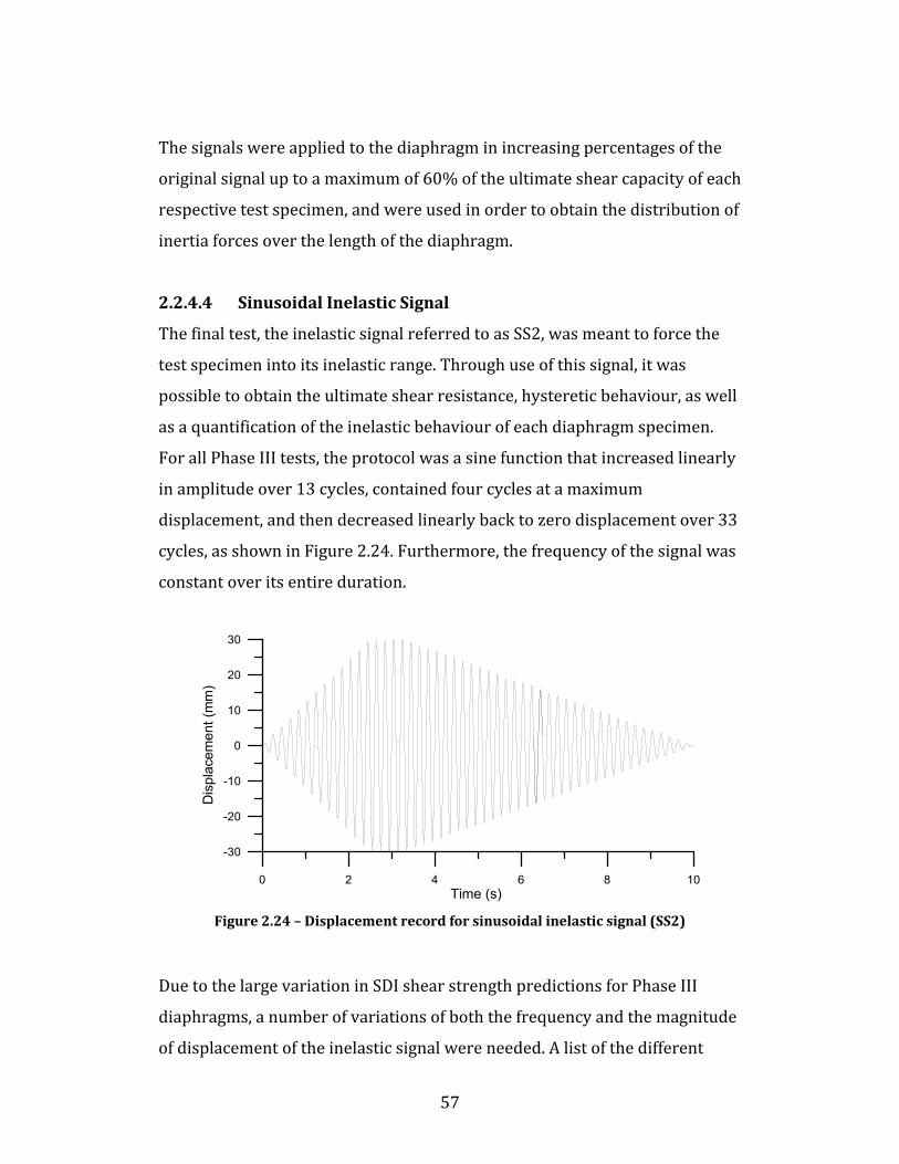
57

The signals were applied to the diaphragm in increasing percentages of the original signal up to a maximum of 60% of the ultimate shear capacity of each respective test specimen, and were used in order to obtain the distribution of inertia forces over the length of the diaphragm. 2.2.4.4 Sinusoidal Inelastic Signal The final test, the inelastic signal referred to as SS2, was meant to force the test specimen into its inelastic range. Through use of this signal, it was possible to obtain the ultimate shear resistance, hysteretic behaviour, as well as a quantification of the inelastic behaviour of each diaphragm specimen. For all Phase III tests, the protocol was a sine function that increased linearly in amplitude over 13 cycles, contained four cycles at a maximum displacement, and then decreased linearly back to zero displacement over 33 cycles, as shown in Figure 2.24. Furthermore, the frequency of the signal was constant over its entire duration.

Figure 2.24 – Displacement record for sinusoidal inelastic signal (SS2) Due to the large variation in SDI shear strength predictions for Phase III diaphragms, a number of variations of both the frequency and the magnitude of displacement of the inelastic signal were needed. A list of the different

0 2 4 6 8 10Time (s)

-30

-20

-10

0

10

20

30

Dis

plac

emen

t (m

m)

58

sinusoidal signals used and the specimens to which they were applied is provided in Table 2.11. The test parameters, both the frequency and magnitude of displacement were selected after an analysis of a model of the specimen developed by Shrestha et al. (2009) was performed in OpenSees (McKenna & Fenves, 2000), that utilized the stiffness properties previously obtained from white noise tests. Table 2.11 – List of sinusoidal inelastic protocols

Inelastic Protocol Specimen 4 Hz, 24 mm DIA15 DIA16 5 Hz, 24 mm DIA11 DIA15R DIA16R DIA17 DIA17R

5 Hz, 27.6 mm DIA12 DIA12R DIA13 DIA18 DIA18R DIA19 DIA19R 5.25 Hz, 27.6 mm DIA13R DIA14 For a complete list of all the tests performed for each of the Phase III specimens, please refer to Appendix B.

2.3 Data Analysis and Methods The following sections describe the methods used in analysing the acquired test data. For this task, two principal programs were used, namely MATLAB (The Mathworks, 2008), a high-level language and computational environment, and Microsoft Office Excel (Microsoft Corporation, 2007). All MATLAB .m files were originally created by Franquet (2010) for Phase I and II analysis and were subsequently modified where necessary for Phase III data.

59

2.3.1 Data Modification and Filtering Occasionally, data recorded from the tests needed to be modified or calibrated due to errors. In a few instances, the instrumentation did not record values or displayed sharp unrealistic spikes and hence needed adjustment. Typically, as the frame was instrumented in a symmetric manner, the values from the same instrument on the other half of the frame were used for this purpose. Recalibration was most often done to accelerometer data where these instruments were at times swapped between series of tests due to errors in measurement. Here, the recorded values were multiplied by a scale factor representing the differences in calibration between the original and replacement instruments. The data obtained from the velocity transducers placed around the frame were processed through a second order Butterworth filter before being analyzed. For these velocity measurements, a high-pass filter was designed to remove a low-frequency drift that was present, and attenuated all frequencies below a level of 0.02 Hz. 2.3.2 Natural Frequency The natural frequency of the diaphragm specimens was obtained using the velocity measurements from the five velocity transducers placed at the end beams and at quarter points of the deck. The modal parameters were obtained using the Frequency Domain Decomposition (FDD) algorithm. This method allows for the determination of mode shapes, damping ratios and fundamental frequencies from the measured response of a structure when subjected to broadband excitation, and also has the advantage of being able to identify closely spaced modes. The basis of this method is that the power spectral density (PSD) of the output can be related to the PSD of the input by the frequency response function (FRF), as shown in Equation 2.3.

60

(2.3) Power spectral density of the output Power spectral density of the input Frequency response function The first step in the algorithm is to evaluate the PSD of the output and to perform singular value decomposition (SVD) at discrete frequencies of the system, shown in Equation 2.4. (2.4) Estimate of the output PSD Unitary matrix holding the singular vectors Diagonal matrix holding the spectral values The fundamental frequencies can then be obtained by using the “peak-picking” technique as a spectral value will dominate at a natural frequency. The corresponding singular vector is then a representation of the mode shape at that frequency. More information on the FDD technique can be found in Brincker et al. (2001). 2.3.3 Resonance Plots Given the velocity data of the sine sweep tests resonance plots were created, as shown in Figure 2.25. The relative velocity of the test specimen at mid-span for each frequency of excitation is plotted, as shown on the left side of the figure. In determining the relative velocity, the average motion of both actuators was used to account for the fact that the two were never acting perfectly in phase. The right side of the figure displays the maximum magnitude of the response at the different frequencies of excitation. The results from the sine sweep tests were able to be compared with results

61

obtained from the white noise testing. A discussion of the findings is presented in Section 2.4.3.

Figure 2.25 – Sine sweep resonance plot example

2.3.4 Damping The resonance curves described in Section 2.3.3 were also meant to provide a means of determining the damping ratios of the diaphragm specimens by using the half-power bandwidth method as described by Chopra (2006). However, due to the difficulty in applying this protocol to even the most flexible of specimens in Phase III, results were frequently not achievable by this method. As such, another method, which utilized the spectral values of the first mode obtained from the white noise analysis, was used. After having determined the singular values for the first mode over a range of frequencies for a particular white noise test using the FDD algorithm, an inverse Fourier transform was performed on those values which exceeded a specified modal assurance criterion (MAC) value of 0.75. With the values now being in the time domain, the peaks of the resulting motion decay could be evaluated and used to determine the logarithmic decrement, δ, and the damping ratio, ζ, tabulated in Section 2.5.2, according to Equations 2.5 and 2.6 respectively. Further discussion of the evaluation of the damping ratios can be found in Franquet (2010) and Brincker et al. (2001).

Time (s)Rel

ativ

e V

eloc

ity a

t Mid

span

(mm

/s)

Frequency (Hz)

Magnitude of S

teady-stateR

esponse

62

2 ln | | (2.5) Initial value of the correlation function k’th extreme of the correlation function ζ √4 (2.6) 2.3.5 Shear Force Calculation The shear force profiles and shear force time histories for various amplitudes of the SS loading protocols were calculated using potentiometer data as well as the calculated mass over a potentiometer’s respective tributary area. By converting the displacement data into accelerations, as the accelerometer readings were found to be unreliable, and multiplying by the mass, the inertia forces in the diaphragm could be computed at a particular location along the width. Finally, the addition of these forces, from zero at the centreline of the frame to the end beam, gave the magnitude of the shear force carried by the diaphragm. The values could then be compared with the force measurements from the load cell after adjusting the latter for an assumption that the weight of the end beam and actuator swivel went directly to the actuator and did not affect the force carried by the diaphragm.

Figure 2.26 – Tributary areas for mass determination of Layout II

m1a0

Fm0a0

m2a3 m3a4 m4a5 m5a6 m6a7 m7a8

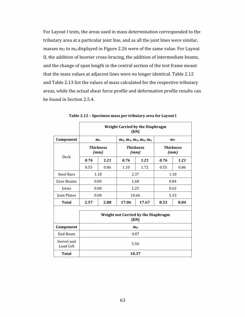
63

For Layout I tests, the areas used in mass determination corresponded to the tributary area at a particular joist line, and as all the joist lines were similar, masses m2 to m6 displayed in Figure 2.26 were of the same value. For Layout II, the addition of heavier cross-bracing, the addition of intermediate beams, and the change of span length in the central section of the test frame meant that the mass values at adjacent lines were no longer identical. Table 2.12 and Table 2.13 list the values of mass calculated for the respective tributary areas, while the actual shear force profile and deformation profile results can be found in Section 2.5.4. Table 2.12 – Specimen mass per tributary area for Layout I

Weight Carried by the Diaphragm

(kN)

Component m1 m2, m3, m4, m5, m6 m7

Deck Thickness (mm)

Thickness (mm)

Thickness (mm)

0.76 1.21 0.76 1.21 0.76 1.21 0.55 0.86 1.10 1.72 0.55 0.86 Steel Bars 1.18 2.37 1.18 Eave Beams 0.84 1.68 0.84 Joists 0.00 1.25 0.62 Joist Plates 0.00 10.66 5.33 Total 2.57 2.88 17.06 17.67 8.53 8.84

Weight not Carried by the Diaphragm

(kN)

Component m0 End Beam 4.87 Swivel and Load Cell 5.50 Total 10.37

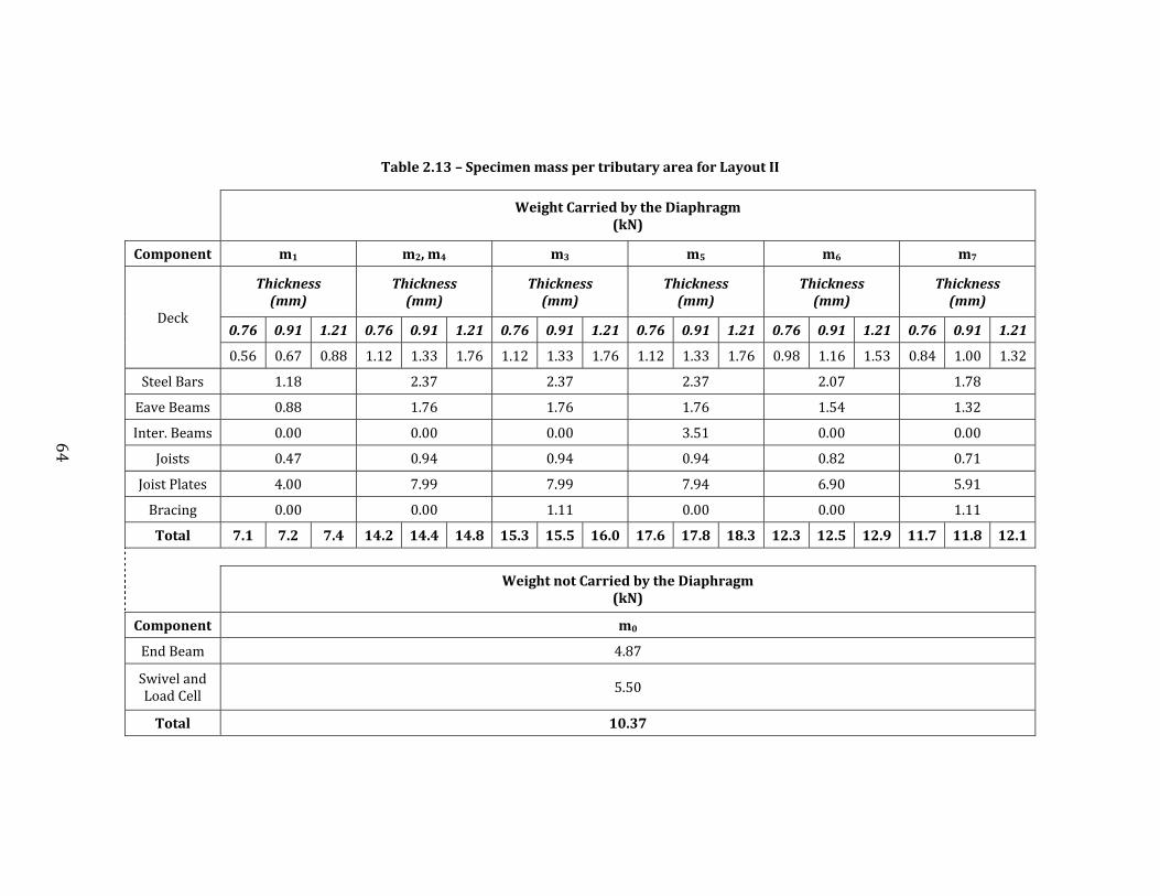
64

Table 2.13 – Specimen mass per tributary area for Layout II

Weight Carried by the Diaphragm (kN)

Component m1 m2, m4 m3 m5 m6 m7 Deck Thickness

(mm) Thickness (mm) Thickness

(mm) Thickness (mm) Thickness

(mm) Thickness (mm)

0.76 0.91 1.21 0.76 0.91 1.21 0.76 0.91 1.21 0.76 0.91 1.21 0.76 0.91 1.21 0.76 0.91 1.210.56 0.67 0.88 1.12 1.33 1.76 1.12 1.33 1.76 1.12 1.33 1.76 0.98 1.16 1.53 0.84 1.00 1.32 Steel Bars 1.18 2.37 2.37 2.37 2.07 1.78 Eave Beams 0.88 1.76 1.76 1.76 1.54 1.32 Inter. Beams 0.00 0.00 0.00 3.51 0.00 0.00 Joists 0.47 0.94 0.94 0.94 0.82 0.71 Joist Plates 4.00 7.99 7.99 7.94 6.90 5.91 Bracing 0.00 0.00 1.11 0.00 0.00 1.11 Total 7.1 7.2 7.4 14.2 14.4 14.8 15.3 15.5 16.0 17.6 17.8 18.3 12.3 12.5 12.9 11.7 11.8 12.1 Weight not Carried by the Diaphragm

(kN) Component m0 End Beam 4.87 Swivel and Load Cell 5.50

Total 10.37

65

Graphs were prepared that show the force profile of the diaphragm at the instant in time when the shear force at a particular joist line reaches its maximum. Since seven such joist lines or tributary areas are considered, and the times at which the maximum forces are obtained may not correspond, seven profiles were possible. Similarly, displacement profiles were created that show the displaced state of the diaphragm at the same instant in time when the maximum shear force was attained. 2.3.6 Shear Force Hystereses The seismic response of the diaphragm specimens was obtained from the application of the sinusoidal inelastic tests, for which the hysteretic response of end shear versus mid-span deflection, and end shear versus end panel deflection was determined. The shear force ratio, S/Sn, at both actuators was calculated following the same procedure as the previously mentioned shear force time histories, represented in Equation 2.7. 7.31 (2.7) Shear force of the diaphragm (kN/m) Force measurement from the actuator load cell (kN) Mass of the end beam, actuator load cell and swivel (kg) Acceleration measured at the location of the end beam (g) For the behaviour at mid-span, potentiometer data was converted to relative displacement by subtracting the magnitude of motion at both actuator locations. This value was then converted to a percentage of the diaphragm’s 21 m length. Two graphs were plotted for every specimen to show the differences in behaviour for both the north and south actuators.

66

2.4 Test Results

2.4.1 Natural Frequency of Specimens Graphs showing the change in the first fundamental period of the diaphragm as a function of the white noise excitation amplitude, chosen to be represented by the root mean square of the acceleration at mid-span, were plotted for all specimens, with that of DIA16 presented in Figure 2.27. In this figure, the diamond points represent the data for all levels of amplification of the white noise signal fitted with a log trend line. The dashed line represents the period, T, calculated using the equations proposed by Medhekar and Kennedy (1997) introduced in Section 1.6.3.1 and repeated in Equations 2.8, and 2.9 for convenience. In using these formulas, the shear stiffness, G’, was determined by matching the longest experimental period with the period of the OpenSees model developed by Shrestha et al. (2009). Additionally, the flexural rigidity of the eave beams, EI, was obtained using the average area of the beams members, including the area of the HSS shear connectors, for the moment of inertia calculation.

Figure 2.27 – Fundamental period as a function of the root mean square of the

response acceleration for DIA16 0 500 1000 1500 2000

RMS Absolute Acceleration (mm/s2)

0.00

0.05

0.10

0.15

0.20

Fund

amen

tal P

erio

d (s

)

DIA16 ResultsLog Fit DIA16TMedhekar (G' = 12.8 kN/mm)

67

2 (2.8) Where (2.9) Stiffness of the lateral braces, considered as infinite Stiffness of the diaphragm Seismic weight of the test specimen, not considering the weight of the end beams or actuator swivel Length of the diaphragm, 21,020 mm Width of the diaphragm, 7,312 mm Young’s modulus of steel Moment of inertia of eave beams, = Ab2/2 Shear stiffness of the diaphragm A second plot, shown in Figure 2.28 for DIA16, which demonstrates the change in stiffness as a function of the applied shear force, both calculated as a ratio of their nominal values as predicted by the SDI method (Luttrell, 2004), was constructed for each specimen using the white noise data. The data points are fitted with a log curve, and were evaluated by solving Equation 2.9 for G’, after having evaluated the diaphragm stiffness, KD, using the measured fundamental period. The point where the experimental values of stiffness and the SDI predictions coincide for a single 7 m long panel are represented by the dashed line, which is used to clearly indicate the levels of excitation for which the SDI prediction is accurate. The plots for all new and repaired diaphragm specimens may be found in Appendix C and Appendix D.

68

Figure 2.28 – Comparison of experimental and predicted stiffness at varying levels of

the predicted strength for DIA16 2.4.2 Damping Ratios The damping ratios were obtained by using the free decay time domain function according to the procedure described in Section 2.3.4. This was calculated for all new diaphragm specimens for the highest amplitude white noise signal. A sample plot for DIA17 is shown in Figure 2.29, with the remaining free decay and damping envelope graphs being included in Appendix E.

Figure 2.29 – Free decay and damping envelope plot of DIA17

0.0 0.2 0.4 0.6S/Sn

0.00

0.50

1.00

1.50

2.00

G' ex

perim

enta

l/G' SD

I

DIA16 ResultsLog Fit DIA16G' = G'SDI

0 2 4 6 8 10Time (s)

-1

-0.5

0

0.5

1

R1(

t) N

orm

aliz

ed

ζ = 0.8%

69

2.4.3 Resonant Frequencies The resonance curves obtained for DIA15 and DIA15R both showed an elongation of the natural frequency of the test specimens with increased loading. For example, a shift in the resonant frequency from 6.25 Hz at a signal amplification of 12.5%, to approximately 5 Hz at an amplification of 100% can be seen in Figure 2.30 for DIA15R. For the sine sweep results, a 100% amplification of the signal corresponds to a motion which induces a peak shear force equal to 20% of the nominal resistance at the specimen ends. For the resonance plot of DIA15, please refer to Appendix F.

Figure 2.30 – Resonance curve plot of DIA15R

2.4.4 Shear Force and Deformation Profiles Shear force profile and deformation profile plots were prepared for each diaphragm specimen for the lowest and highest amplifications of the SS1 and SS3 signals, as well as for the inelastic SS2 signal. The graphs represent an instant in time when the shear force at a particular joist line (or potentiometer location for Layout II tests) reaches a maximum. Figure 2.31 displays the plots obtained for DIA11 for the highest amplitude of the SS2 inelastic signal. The remaining graphs representing the shear force and deformation profiles can be found in Appendix G and Appendix H.

4 4.5 5 5.5 6 6.5Frequency of Excitation (Hz)

0

10

20

30

40

50

Rel

ativ

e V

eloc

ity a

t Mid

-Spa

n (m

m/s

)

12.5% Amplification25.0% Amplification37.5% Amplification50.0% Amplification62.5% Amplification75.0% Amplification87.5% Amplification100% Amplification

70

Shear Force Determined with Actuator MeasurementsShear Force Determined with Inertia Forces

Figure 2.31 – Shear force and deformation profile plot of DIA11 Shear force time histories were also plotted in order to compare the shear force calculated by summing the inertia forces to the data acquired from the load cells after subtracting the force due to the end beam and load cell swivel. The acceleration measurements used in this calculation were obtained by double integration of the displacement values due to inconsistency of the accelerometer readings. A typical result can be seen in Figure 2.32.

Figure 2.32 – Shear force time history plot for DIA11, SS1 signal

0 2 4 6Location

0

40

80

120

160

200

Shea

r For

ce, S

u*7.

31 (k

N)

SS2-80

0 2 4 6Location

0

10

20

30

40

Def

orm

atio

n (m

m)

Sheet Overlaps

Location0 1 2 3 4 5 6

End BeamJoist 1Joist 2Joist 3Joist 4Joist 5Joist 6

4 6 8 10 12Time (s)

-30

-20

-10

0

10

20

30

She

ar F

orce

(kN

)

71

2.4.5 Inelastic Behaviour The inelastic performance of the diaphragm specimens could be evaluated by observing the shear force vs. mid-span displacement hystereses, shear force vs. end panel displacement, as well as the connector damage patterns for the SS2 inelastic protocol. Two such hystereses are shown in Figure 2.33 for specimen DIA11, where the left graphs demonstrates the behaviour at the north actuator, and the right graph demonstrates the south. The end panel, for Layout I tests is located at the first joist line, at a distance of 1,752 mm from the end beam. For Layout II, the end panel is taken as the second sidelap location, at a distance of 1,828 mm from the end beam. These particular locations were selected for the hystereses as the maximum shear and inelastic response of the specimens was concentrated at the ends of the test frame. For the end-panel hystereses, the value, γ, is equal to the relative displacements at both ends of the end zone panel length divided by the total length of the end panel. The remaining hystereses for mid-span displacement may be consulted in Appendix I for all new diaphragm specimens and in Appendix J for repaired specimens. After every inelastic test, each connector was examined for damage with the results tabulated in Appendix K. In these figures, every connection from south to north (left to right) and west to east (top to bottom) is represented by a single square. Where squares are not filled, the connections were determined to be intact after the inelastic signal, while damaged connections are represented following the information provided in Table 2.14. Additionally, figures representing the masses that were dislodged or loosened during the inelastic test can be found for every specimen.

72

Figure 2.33 – Shear force vs. displacement hystereses at mid-span (top) and end panel

(bottom) of DIA11 Table 2.14 – Representation of connector damage

Symbol Type of Damage X Nail/screw removal O Nail/screw bearing failure Nail excessive slotting failure Y Weld bearing failure P Weld sheet tearing failure Further discussion of the observed connector damage, as well as the inelastic behaviour is presented in Section 2.5.5.

-0.3 -0.2 -0.1 0 0.1 0.2 0.3δm/L (x102)

-2

-1

0

1

2

S 1/S

u

-0.3 -0.2 -0.1 0 0.1 0.2 0.3δm/L (x102)

-2

-1

0

1

2

S2/S

u

-8 -4 0 4 8γ (mRad)

-2

-1

0

1

2

S1/S

u

-8 -4 0 4 8γ (mRad)

-2

-1

0

1

2

S2/S

u

73

2.5 Discussion of Results The following section provides an in-depth evaluation of the findings from the experimental testing program, and has been separated into the following topics: diaphragm stiffness, damping, shear force and deformation, shear strength, inelastic behaviour, and repair strategies. 2.5.1 Diaphragm Shear Stiffness As discussed previously, the stiffness properties of the diaphragm specimens were obtained using the SDI method (Luttrell, 2004) for a 7 m panel, along with the nominal fastener and material properties (Case A in Table 2.7). The stiffness values obtained from the dynamic tests at different levels of excitation are shown in Table 2.15. Here, the ambient level, G’0%, performed prior to white-noise tests, approximately corresponds to an average excitation level equal to 1% or less of the ultimate shear resistance of the diaphragm, while the 20% level, G’20%, corresponds to 20% of the shear resistance and was typically attained during the largest amplitude white-noise test. Finally, the experimental level, G’EXP, implies an average value of approximately 40% of the SDI shear resistance, and was obtained at the highest amplification of either of the SS1 or SS3 signals. The stiffness values are related to the fundamental period of the specimens through Medhekar’s equation (Medhekar & Kennedy, 1997) presented in Section 2.4.1, and were calculated by solving for the stiffness of the diaphragm, Kd, using the measured period of the test specimens at the various amplitudes. With this relationship, the elongation of the period shown by the white-noise tests translates into a corresponding decrease in shear stiffness. As can be seen, all the specimens showed a decrease in stiffness from the beginning to the end of white-noise tests, with the stiffness further decreasing once the specimen was subjected to the larger SS1 and SS3 loading protocols. Although all specimens decreased in stiffness through

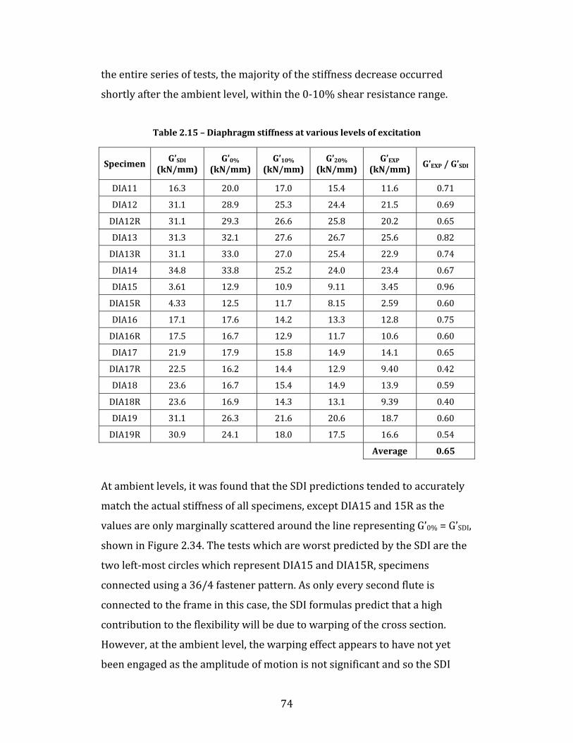
74

the entire series of tests, the majority of the stiffness decrease occurred shortly after the ambient level, within the 0-10% shear resistance range. Table 2.15 – Diaphragm stiffness at various levels of excitation

Specimen G’SDI

(kN/mm) G’0%

(kN/mm) G’10%

(kN/mm) G’20%

(kN/mm) G’EXP

(kN/mm) G’EXP / G’SDI DIA11 16.3 20.0 17.0 15.4 11.6 0.71 DIA12 31.1 28.9 25.3 24.4 21.5 0.69 DIA12R 31.1 29.3 26.6 25.8 20.2 0.65 DIA13 31.3 32.1 27.6 26.7 25.6 0.82 DIA13R 31.1 33.0 27.0 25.4 22.9 0.74 DIA14 34.8 33.8 25.2 24.0 23.4 0.67 DIA15 3.61 12.9 10.9 9.11 3.45 0.96 DIA15R 4.33 12.5 11.7 8.15 2.59 0.60 DIA16 17.1 17.6 14.2 13.3 12.8 0.75 DIA16R 17.5 16.7 12.9 11.7 10.6 0.60 DIA17 21.9 17.9 15.8 14.9 14.1 0.65 DIA17R 22.5 16.2 14.4 12.9 9.40 0.42 DIA18 23.6 16.7 15.4 14.9 13.9 0.59 DIA18R 23.6 16.9 14.3 13.1 9.39 0.40 DIA19 31.1 26.3 21.6 20.6 18.7 0.60 DIA19R 30.9 24.1 18.0 17.5 16.6 0.54 Average 0.65 At ambient levels, it was found that the SDI predictions tended to accurately match the actual stiffness of all specimens, except DIA15 and 15R as the values are only marginally scattered around the line representing G’0% = G’SDI, shown in Figure 2.34. The tests which are worst predicted by the SDI are the two left-most circles which represent DIA15 and DIA15R, specimens connected using a 36/4 fastener pattern. As only every second flute is connected to the frame in this case, the SDI formulas predict that a high contribution to the flexibility will be due to warping of the cross section. However, at the ambient level, the warping effect appears to have not yet been engaged as the amplitude of motion is not significant and so the SDI

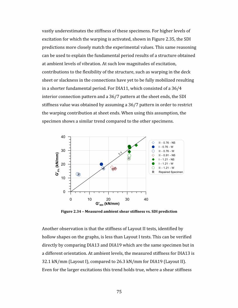
75

vastly underestimates the stiffness of these specimens. For higher levels of excitation for which the warping is activated, shown in Figure 2.35, the SDI predictions more closely match the experimental values. This same reasoning can be used to explain the fundamental period results of a structure obtained at ambient levels of vibration. At such low magnitudes of excitation, contributions to the flexibility of the structure, such as warping in the deck sheet or slackness in the connections have yet to be fully mobilized resulting in a shorter fundamental period. For DIA11, which consisted of a 36/4 interior connection pattern and a 36/7 pattern at the sheet ends, the SDI stiffness value was obtained by assuming a 36/7 pattern in order to restrict the warping contribution at sheet ends. When using this assumption, the specimen shows a similar trend compared to the other specimens.

Figure 2.34 – Measured ambient shear stiffness vs. SDI prediction Another observation is that the stiffness of Layout II tests, identified by hollow shapes on the graphs, is less than Layout I tests. This can be verified directly by comparing DIA13 and DIA19 which are the same specimen but in a different orientation. At ambient levels, the measured stiffness for DIA13 is 32.1 kN/mm (Layout I), compared to 26.3 kN/mm for DIA19 (Layout II). Even for the larger excitations this trend holds true, where a shear stiffness

1:1

0 10 20 30 40G'SDI (kN/mm)

0

10

20

30

40

G' 0%

(kN

/mm

)

II - 0.76 - NSI - 0.76 - WII - 0.76 - WII - 0.91 - NSI - 1.21 - NSI - 1.21 - WII - 1.21 - WRepaired Specimen

76

of 25.6 kN/mm for DIA13, compared with 18.7 kN/mm for DIA19, is measured. Although these two tests were the only ones in Phase III of the diaphragm experiments which can be compared in this way, overlap with Phase II results (Franquet, 2010) confirms this trend. This is due to the fact that in Layout II specimens, the two free sheet ends which cannot be overlapped due to the modified frame orientation, contribute more warping flexibility than in Layout I. It must be noted that G’SDI was determined based on the assumption that each of the three sheets along the diaphragm length in Layout I was free to warp at both its ends. In fact, warping is partially restricted at the overlapped joints, as warping deformations of the two individual sheets at the joints develop in opposite directions and are restrained by the fact that the two sheets overlap. In Table 2.7, the G’ value from Case B corresponds to the extreme case where zero warping is assumed at the overlapped joints. When comparing test results to the Case B predictions the SDI is seen to even more greatly overestimate the stiffness of the specimens implying that an overlap with no warping distortions may not be an accurate assumption. Stiffness graphs for all diaphragm specimens from Phases I, II and III of testing are included in Appendix L.

Figure 2.35 – Measured experimental shear stiffness vs. SDI prediction

0.67:1

1:1

0 10 20 30 40G'SDI (kN/mm)

0

10

20

30

40

G' EX

P (kN

/mm

)

II - 0.76 - NSI - 0.76 - WII - 0.76 - WII - 0.91 - NSI - 1.21 - NSI - 1.21 - WII - 1.21 - WRepaired Specimen

77

At high amplitudes, the average stiffness of Phase III diaphragm specimens compared to the SDI was 0.65 (0.67 when including tests from all three phases). Such a variation between the two values may be due to the fact that the diaphragm specimens were tested numerous times prior to reaching the experimental level where the stiffness was evaluated. Additionally, possible slackness or minor damage may have accumulated at the connections from these previous tests resulting in specimens that are more flexible than would normally be assumed. These numerous lower level elastic tests may be similar to what will occur on an actual single storey structure due to wind loads, where over many years, a structure could be subjected to hundreds of cycles of loading and unloading. 2.5.2 Damping The damping ratios, ζ, calculated according to Section 2.3.4 are included in Table 2.16 for the new diaphragm specimens. The damping values for steel structures are usually found within the range of 2-7%. As the average of the tests was 2.2%, the results agree well. Had non-structural roofing components been attached to the roof diaphragm in the lab, the level of damping would have likely increased. There appears to be little difference in the damping values when comparing between layouts, and the higher damping values obtained for tests that were connected using welds and button-punches agrees with the results from Phase II (Franquet, 2010), where DIA10, a Layout I welded and button-punched specimen was found to have a damping ratio of 6.6%. This was attributed to the high amount of friction and sliding in the button-punch sidelap connections which, according to the SDI formulas (Luttrell, 2004), are approximately ten times more flexible than a screwed connection for 0.76 mm thick deck. Additionally, both specimens connected using a 36/4 frame fastener pattern, DIA11 and DIA15, may have experienced more friction between the steel frame and the larger warping deformations of the cross section at the sheet ends.

78

Table 2.16 – Diaphragm damping ratios

SpecimenDamping Ratio, ζ

(%) DIA11 4.0 DIA12 1.8 DIA13 2.4 DIA14 1.9 DIA15 5.3 DIA16 1.1 DIA17 0.8 DIA18 1.1 DIA19 1.8 Average 2.24

2.5.3 Shear Force and Deformation Profiles The majority of the diaphragm specimens exhibited the trends for both shear force profile and deformed shape that are shown in Figure 2.36. The plots were obtained by first normalizing the shear forces of a test, either elastic or inelastic, to the maximum shear experienced for the same test, and then averaging the normalized values for all Phase III specimens.

Figure 2.36 – Average normalized shear force and deformation profiles for elastic and

inelastic tests 0 0.1 0.2 0.3 0.4 0.5 0.6

x/L

0.0

0.2

0.4

0.6

0.8

1.0

1.2

Nor

mal

ized

Def

orm

atio

nat

Max

imum

She

ar

Inelastic Envelope

0 0.1 0.2 0.3 0.4 0.5 0.6x/L

0.0

0.2

0.4

0.6

0.8

1.0

1.2

Nor

mal

ized

She

ar F

orce

Elastic Envelope

79

The common design convention for a simply-supported structure is to assume that the earthquake induced lateral shear force varies linearly over the length of the building. The experimental results on the other hand, show more of a parabolic variation with the shear values at the end and at the first joist line, represented by x/L = 0.08, being approximately equal. With respect to deformation, the highest demand occurs between the end beam and the first joist line, where the deformation reaches 35-40% of the total measured displacement. The deformed shape resembles a parabola for the higher amplitude elastic and inelastic protocols. The findings of a more parabolic shear force profile corresponds with the findings by Tremblay and Stiemer (1996) and Tremblay et al. (2000). 2.5.4 Diaphragm Shear Strength The experimental versus predicted strength of all Phase III diaphragm specimens is listed in Table 2.17 and shown in Figure 2.37. It was determined that all new specimens were able to achieve and even surpass their SDI (Luttrell, 2004) shear strength predictions, which, much like the shear stiffness calculations were obtained by using the nominal properties of the steel deck. If an adjustment is made to account for the actual value of Fu, the ultimate tensile stress as measured from coupon tests, the Su/Sn values correspondingly drop to an average of 1.09, a value close to unity which indicates that the SDI strength predictions are accurate if the actual Fu value of the steel is known. For the repaired specimens, all but one, DIA15R, were able to attain their predicted shear strengths. If the performance of the repaired specimens is evaluated with respect to the strength predictions of the new diaphragms, they are seen to perform quite well. What this means is that even though a repaired specimen, such as DIA15R, may not be able to achieve the SDI strength prediction because of residual damage, repaired specimens always provided an upgrade in shear strength from their initial configurations. It

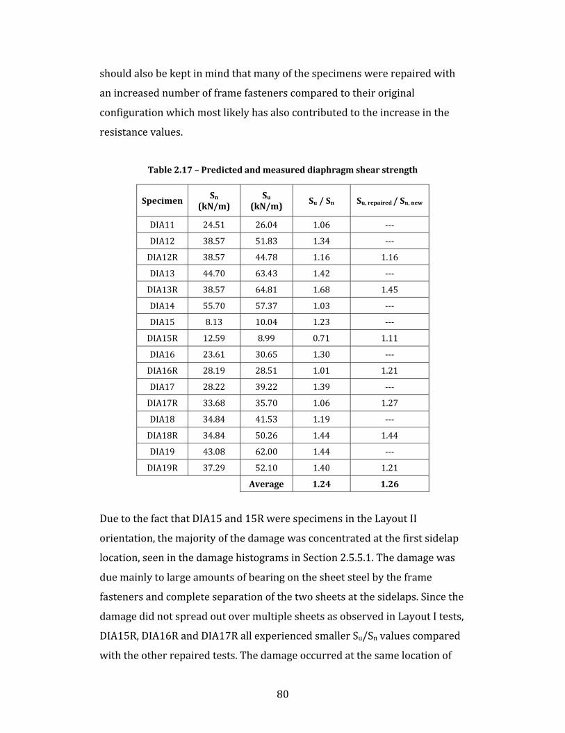
80

should also be kept in mind that many of the specimens were repaired with an increased number of frame fasteners compared to their original configuration which most likely has also contributed to the increase in the resistance values. Table 2.17 – Predicted and measured diaphragm shear strength

Specimen Sn

(kN/m) Su

(kN/m) Su / Sn Su, repaired / Sn, new DIA11 24.51 26.04 1.06 --- DIA12 38.57 51.83 1.34 --- DIA12R 38.57 44.78 1.16 1.16 DIA13 44.70 63.43 1.42 --- DIA13R 38.57 64.81 1.68 1.45 DIA14 55.70 57.37 1.03 --- DIA15 8.13 10.04 1.23 --- DIA15R 12.59 8.99 0.71 1.11 DIA16 23.61 30.65 1.30 --- DIA16R 28.19 28.51 1.01 1.21 DIA17 28.22 39.22 1.39 --- DIA17R 33.68 35.70 1.06 1.27 DIA18 34.84 41.53 1.19 --- DIA18R 34.84 50.26 1.44 1.44 DIA19 43.08 62.00 1.44 --- DIA19R 37.29 52.10 1.40 1.21 Average 1.24 1.26 Due to the fact that DIA15 and 15R were specimens in the Layout II orientation, the majority of the damage was concentrated at the first sidelap location, seen in the damage histograms in Section 2.5.5.1. The damage was due mainly to large amounts of bearing on the sheet steel by the frame fasteners and complete separation of the two sheets at the sidelaps. Since the damage did not spread out over multiple sheets as observed in Layout I tests, DIA15R, DIA16R and DIA17R all experienced smaller Su/Sn values compared with the other repaired tests. The damage occurred at the same location of

81

the previous inelastic test and appears to have been negatively influenced by the damage already present in the sheets.

Figure 2.37 – Measured vs. predicted shear strength for all Phase III specimens For DIA18, the tailored specimen, damage spread out over nearly the entire test specimen and hence the damage at the first sidelap location was not as extensive as the previously mentioned specimens, such as DIA17 which had the same sheet thickness and fastener types. DIA18R, therefore experienced a larger Su/Sn ratio than the other Layout II, nail/screw repaired specimens. DIA18 was also able to achieve the SDI predicted strength based on the fasteners at the end panel despite having the fastener pattern change over its length. Varying the connections in this manner may provide a more economical way to design a diaphragm.

0 10 20 30 40 50 60Sn (kN/m)

0.00.20.40.60.81.01.21.41.61.8

S u/S

n

II - 0.76 - NSI - 0.76 - WII - 0.76 - WII - 0.91 - NSI - 1.21 - NSI - 1.21 - WII - 1.21 - WRepaired Specimen

82

2.5.5 Diaphragm Inelastic Behaviour

2.5.5.1 Failure Modes The failure modes for individual connectors were similar in both frame layouts and are shown in Figure 2.38. The modes are: 1. Sheet distortion: this failure mode occurred more commonly in thinner sheets close to nailed or welded frame fasteners in the form of local buckling of the sheet bottom flange. It was more pronounced at frame connections along sidelaps, where one of the two overlapped sheets had a free edge, or at the sheet corners where two perpendicular sheet edges were free to move upward. 2. Nail bearing and slotting: constant bearing of the sheet steel against nail fasteners would create slotting deformations in the deck for all thickness specimens. Slotting deformations in the deck occurred in a direction transverse to the deck flutes due to the transfer of shear. 3. Nail failure: a pullout nail failure would typically occur for thicker deck sheets, and most commonly occurred at sidelaps or end overlaps where the fastener had to pass through multiple sheets to fasten to the steel below. Nail shear failures were not observed for Phase III specimens, however did occur infrequently at joist locations during Phase II tests. 4. Screw bearing: the relative movements of two adjacent deck sheets caused this failure for all specimens fastened using sidelap screws. The screws would tilt and bear on the sheet steel, and in some instances become free from the sheet if the bearing deformations were excessive. Tilting occurred in a direction parallel to the flute due to longitudinal shear transfer between sheets.

83

5. Weld bearing: unlike nail fasteners, the bearing of the steel on a weld did not cause slotting deformations. Rather, for thinner steels, the bearing was usually accompanied by slight buckling of the sheet near the weld, while for thicker materials, the connection of the steel around the weld would fail by becoming free around the perimeter of the connection. 6. Weld sheet tearing: this failure mode was caused by shear forces inducing tension on one side of the weld with the sheet tearing in a direction perpendicular to the applied load, as described in Guenfoud et al. (2010). Weld sheet tearing was much more common in thinner deck specimens. 7. Button-punch separation: all 0.76 mm specimens fastened with button-punches experienced this failure mode. The relative movements of two adjacent sheets at their sidelap connections caused a gradual loosening of the connection. The percentage of connectors damaged at sidelap and frame locations along the length of the specimens was calculated, and can be seen for DIA11, DIA14, DIA17 and DIA18 in Figure 2.39. These damage histograms give an indication as to where the majority of the damage occurred, and the type of failure mode a particular specimen experienced. Tests such as DIA11, where the damage spread throughout the entire first sheet were more ductile in nature than for example, DIA14, where nearly all fasteners at one particular location were lost in a sudden manner. From the information provided by the damage histograms, a variable, xfailure, that represents the distance from the end beam to the centre-of-gravity of damage for the side on which the most damage occurred could be calculated, and is found in Figure 2.40.

84

Figure 2.38 – Typical fastener failure modes

2

3

1

4

5 6

7

85

Figure 2.39 – Shear force vs. deformation hystereses and inelastic damage patterns for a) DIA11, b) DIA14, c) DIA17 and d) DIA18

0 0.2 0.4 0.6 0.8 1x/L

0

20

40

60

80

100

0 0.2 0.4 0.6 0.8 1x/L

0

20

40

60

80

100

% F

aile

d O

ver W

idth

0 0.2 0.4 0.6 0.8 1x/L

0

20

40

60

80

100

Frame FastenersSidelap Fasteners

0 0.2 0.4 0.6 0.8 1x/L

0

20

40

60

80

100

% F

aile

d O

ver W

idth

-10 -5 0 5 10γ (mRad)

-45

-30

-15

0

15

30

45

-10 -5 0 5 10γ (mRad)

-45

-30

-15

0

15

30

45

S u (k

N/m

)

-15 -10 -5 0 5 10 15γ (mRad)

-80-60-40-20

020406080

-15 -10 -5 0 5 10 15γ (mRad)

-30

-20

-10

0

10

20

30

S u (k

N/m

)

Positive Envelope for Energy CalculationNegative Envelope for Energy Calculation

Experimental DataExtrapolation for γu

γu

a) b)

c) d)

86

Figure 2.40 –Damage distribution during inelastic test In Layout I, the 0.76 mm thick specimens were much better able to spread the damage throughout the first four sidelap connections than were the thicker 1.21 mm decks. DIA14 for example, with 1.21 mm thick deck sheets in Layout I, shows a high concentration of failure only at the frame fasteners of one end and no damage at all in the sidelaps, which is less desirable than the behaviour observed for the 0.76 mm counterpart (DIA11). Although there was only one 0.76 mm and no 0.91 mm thick specimens tested in Layout I for Phase III, the Phase I and II specimens, which thoroughly covered these thicknesses, showed a higher degree of damage distribution than the 1.21 mm thick specimens. Additionally, when compared to Layout I, Layout II specimens experienced relatively more concentrated damage patterns, comparable to the majority of the 1.21 mm thick specimens. This is seen in Figure 2.39, where DIA17 (Layout II, 0.91 mm) is shown to have damage that spreads only within the two sheets nearest to the end beam. Again, the typical failure mode of Layout II tests was a sudden failure of the sidelap connections of the sheet nearest to the end beam on one side of the test specimen, except for DIA18. This tailored specimen performed much better with regards to distributing the damage than any of the 18 other specimens tested. A centre-of-failure graph for all specimens is included in Appendix L.

0 10 20 30 40 50 60Sn (kN/m)

0

1

2

3

4

x fai

lure

(m)

0

5

10

15

x fai

lure

/L (%

)

II - 0.76 - NSI - 0.76 - WII - 0.76 - WII - 0.91 - NSI - 1.21 - NSI - 1.21 - WII - 1.21 - WRepaired Specimen

87

2.5.5.2 Inelastic Deformation Capacity Shear force versus deformation hystereses at the end panel are provided for selected specimens in Figure 2.39, with mid-span displacement hystereses for all Phase III specimens available in Appendix I and Appendix J. Table 2.18 provides a summary of the inelastic properties measured for Phase III diaphragm specimens calculated from the end panel hystereses. A brief explanation of the parameters examined in this section is presented.

γy: Yield shear strain (mRad) The yield shear strain represents the shear strain reached when a line drawn from the origin, with a slope equal to the local stiffness of the test specimen, reaches the ultimate shear resistance, Su. The selection of the local stiffness was based on the first few elastic cycles of the diaphragm’s response to the inelastic loading protocol.

γu: Ultimate shear strain (mRad) The ultimate shear strain was calculated at the point when the shear resistance of the diaphragm first degraded to a value of 0.8 Su, a generally accepted limit beyond which failure is said to have occurred. Extrapolation for γu: In some instances, the specimen may not have been pushed far enough in the same displacement cycle to reach the ultimate shear strain. For these instances, a linear extrapolation was used to estimate the value of γu, shown, for example in Figure 2.39a.

γp: Plastic shear strain (mRad) The plastic shear strain is equal to γu- γy, and represents the amount of plastic shear deformation achieved by the specimens.

88

Envelopes for energy calculation: The envelope is used to represent an approximation of the amount of energy dissipated for each test. The actual normalized energy calculation was done by adding up the area underneath the load vs. deflection curve until the moment in time when the ultimate deformation, γu, was reached. This value was then normalized with respect to Su multiplied by the sum of the absolute values of the total shear deformations experienced by the specimen from the beginning of the test until the time at which the specimen failed (0.8 Su). The envelope also indicates the value of γy, and an approximate value for γu which is taken as the ordinate of the experimental data point that falls nearest to a shear value of 0.8 Su. This value will differ from γu as listed in Table 2.18 if no data point corresponding to 0.8 Su was acquisitioned during testing. The time at which this measurement is taken also corresponds to the last value used for the energy summation. With respect to the inelastic deformation capability, γu-γy, Layout I specimens were able to undergo greater inelastic deformations than the specimens in Layout II, which experienced a large concentration of demand at a single sidelap location. From Figure 2.41, which represents the ultimate strain values of all Phase I, II and III specimens, it can be seen that Layout II specimens with 0.76 mm and 0.91 mm deck sheets were only able to achieve an ultimate shear strain of approximately 6.0 mRad, compared to 10.9 mRad for the same thickness in the Layout I orientation. The specimens constructed of 1.21 mm thick deck sheets also performed poorly compared to the 0.76 mm and 0.91 mm specimens tested in Phase I and II, where the ultimate shear strain reached was on the order of 12 to 19 mRad (Franquet, 2010).

89

Table 2.18 – Summary of inelastic properties

Specimenγy

(mRad) γu

(mRad) γp

(mRad)γu / γy

Normalized Energy Dissipated DIA11 2.7 10.9 8.2 4.0 0.21 DIA12 1.9 8.5 6.6 4.5 0.31 DIA12R 1.4 7.4 6.0 5.1 0.32 DIA13 2.0 6.6 4.6 3.4 0.25 DIA13R 2.2 10.6 8.4 4.8 0.28 DIA14 1.9 6.1 4.2 3.2 0.24 DIA15 2.7 5.5 2.8 2.0 0.23 DIA15R 4.7 5.9 1.2 1.3 0.12 DIA16 1.7 6.5 4.8 3.8 0.19 DIA16R 2.3 5.3 3.0 2.3 0.19 DIA17 2.1 5.0 2.9 2.4 0.13 DIA17R 2.4 5.3 2.9 2.3 0.14 DIA18 2.3 5.0 2.8 2.2 0.16 DIA18R 3.4 8.1 4.8 2.4 0.17 DIA19 2.8 6.1 3.4 2.2 0.12 DIA19R 2.6 8.3 5.7 3.2 0.16

Average 2.4 7.0 4.5 3.1 0.20

Figure 2.41 – Ultimate shear strain for all Phase I, II and III specimens

0 10 20 30 40 50 60Sn (kN/m)

02468

101214161820

γ u (m

Rad

)

I - 0.76 - NSII - 0.76 - NSI - 0.76 - WII - 0.76 - WI - 0.91 - NSII - 0.91 - NSI - 1.21 - NSI - 1.21 - WII - 1.21 - W

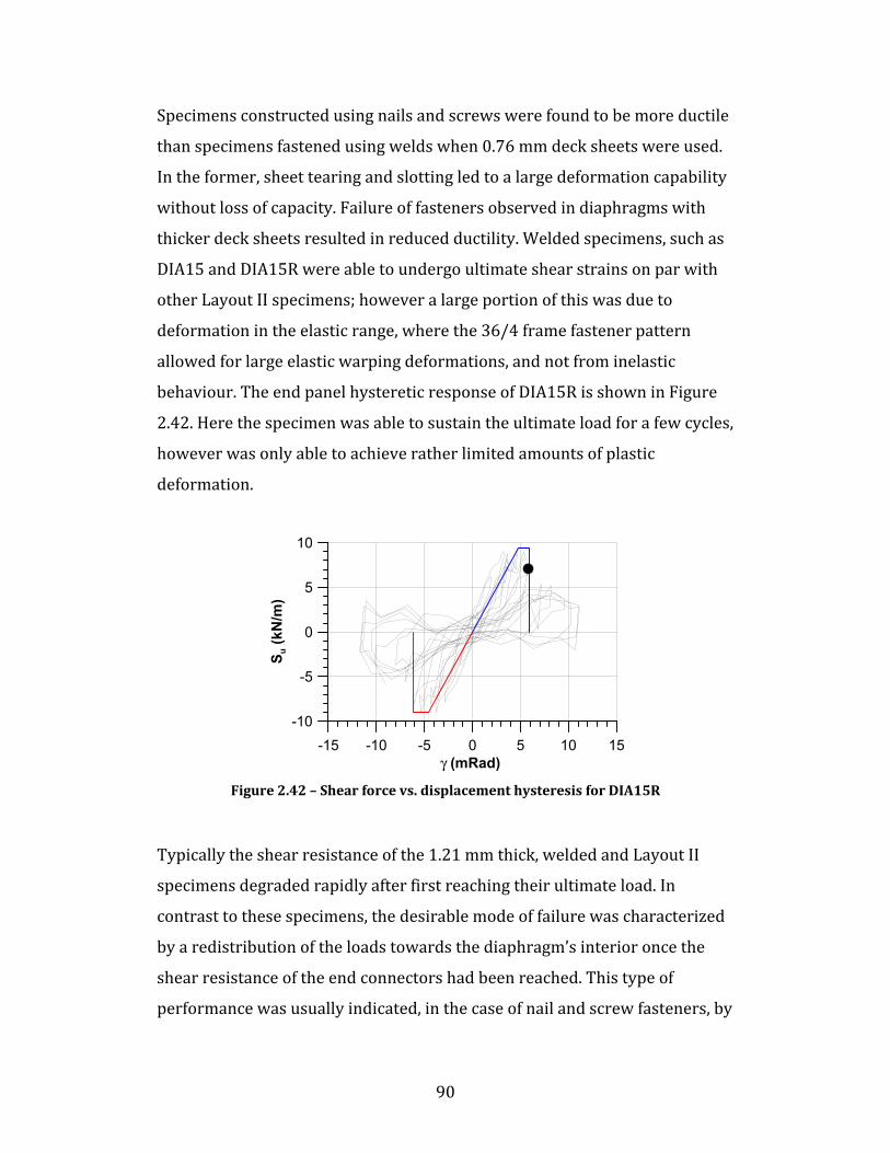
90

Specimens constructed using nails and screws were found to be more ductile than specimens fastened using welds when 0.76 mm deck sheets were used. In the former, sheet tearing and slotting led to a large deformation capability without loss of capacity. Failure of fasteners observed in diaphragms with thicker deck sheets resulted in reduced ductility. Welded specimens, such as DIA15 and DIA15R were able to undergo ultimate shear strains on par with other Layout II specimens; however a large portion of this was due to deformation in the elastic range, where the 36/4 frame fastener pattern allowed for large elastic warping deformations, and not from inelastic behaviour. The end panel hysteretic response of DIA15R is shown in Figure 2.42. Here the specimen was able to sustain the ultimate load for a few cycles, however was only able to achieve rather limited amounts of plastic deformation.

Figure 2.42 – Shear force vs. displacement hysteresis for DIA15R Typically the shear resistance of the 1.21 mm thick, welded and Layout II specimens degraded rapidly after first reaching their ultimate load. In contrast to these specimens, the desirable mode of failure was characterized by a redistribution of the loads towards the diaphragm’s interior once the shear resistance of the end connectors had been reached. This type of performance was usually indicated, in the case of nail and screw fasteners, by

-15 -10 -5 0 5 10 15γ (mRad)

-10

-5

0

5

10

S u (k

N/m

)

91

a pinched hysteretic behaviour where the steel deck would bear on the frame fasteners causing slotting and the sidelap fasteners would tilt and gradually loosen. Such a failure mode, which can be considered desirable, occurred for the majority of the 0.76 mm and 0.91 mm Layout I specimens tested by Franquet (2010). The results of the normalized values of energy dissipation are compiled for Phase III specimens in Figure 2.43, and for all new diaphragm specimens in Appendix L. Similar to the other properties already discussed, the Layout II specimens are found to dissipate less energy for a given strength and shear strain than their Layout I counterparts. When comparing amongst all Phase I, II and III specimens, it was seen that welded specimens with button-punch sidelaps did not dissipate as much energy as the same thickness specimens connected with nails and screws. Due to their poor inelastic performance, 0.76 mm welded and button-punch specimens would thus not appear to be suitable as the fuse element in a seismic force resisting system. The 1.21 mm specimens fastened with welds and screws performed similarly to those fastened using nails and screws, however, in general, the 1.21 mm specimens, regardless of the fastener type were more brittle than the specimens constructed using thinner deck sheets.

Figure 2.43 – Normalized energy dissipated for all Phase III specimens

0 10 20 30 40 50 60Sn (kN/m)

0.0

0.1

0.2

0.3

0.4

Nor

mal

ized

Ene

rgy

Dis

sipa

ted

II - 0.76 - NSI - 0.76 - WII - 0.76 - WII - 0.91 - NSI - 1.21 - NSI - 1.21 - WII - 1.21 - WRepaired Specimen

92

2.5.6 Retrofit and Repair Strategies

2.5.6.1 Nail and Screw Repairs Three out of four of the nail and screw repaired specimens, DIA12R, DIA16R and DIA17R were found to be weaker than when tested in their new state. DIA18R, which had a constant fastener pattern over its length, was an upgrade to DIA18 and showed an improvement in strength although both specimens were able to achieve their SDI prediction. Stiffness was almost completely regained for specimens DIA12R and DIA16R, with the small difference likely caused by the damage present in the repaired specimen from the initial inelastic test. A similar effect was in play for DIA17R, as the initial damage for this specimen was very highly concentrated at all fasteners around the first sidelap location. Damage from the initial inelastic test included many instances of the steel sheet tearing around a nail which may have been responsible for the more exaggerated loss in stiffness. Finally, DIA18R was found to be more flexible than DIA18 even though it contained a greater number of fasteners towards its centre. This appears to confirm the results from modelling that the stiffness of a diaphragm is more heavily influenced by the behaviour of the end panel, as shown in Figure 2.44. In this figure, the end panels of DIA18R were found to be more flexible most likely due to the damage present from the initial inelastic test, as even though the damage for DIA18 was spread over the entire specimen, nearly 100% of the end panel fasteners failed on one side of the specimen during the inelastic test. The higher stiffness at the centre of DIA18R does not seem to play a significant role in its overall behaviour.

93

Figure 2.44 – Schematic of flexible end panel for DIA18R

2.5.6.2 Weld and Button-punch Repair and Retrofit The retrofitted specimen, DIA11, saw a significant increase in strength compared with the equivalent non-retrofitted specimen from Phase II, DIA10 as shown in Figure 2.45. The change in strength is due to two factors. Firstly, the retrofitted specimen contained both 16 mm weld and nail fasteners acting together in an undamaged state, which had the effect of nearly doubling the overall resistance of the frame fasteners. Secondly, the fasteners at end overlaps were increased to a 36/7 pattern in DIA11 from a 36/4 pattern in DIA10, again contributing to an increased in-plane shear resistance. The stiffness also increased for the retrofit from a value of 3.6 kN/mm for DIA10 to 11.6 kN/mm for DIA11 respectively. This increase in stiffness can largely be attributed to the use of the steel strip and screws installed at the sidelap connections, as well as the increase in frame fastener pattern from 36/4 to 36/7. As opposed to the button-punches which rely heavily on the interlocking and friction of two adjacent sheets, the screws and steel strip provide a more secure mechanical connection that restricts the sheets from acting independently.

Rigid central panels

Flexible end panel

94

Figure 2.45 – End panel hystereses of DIA10R, DIA11 and DIA15R The screwed steel strip method was also used to repair a specimen, DIA15R, in Layout II. The new specimen, which was connected using button-punches at the sidelaps, failed very rapidly during the inelastic SS2 signal. Here, the low strength of the sidelaps caused an especially sudden failure with little inelastic deformation capability. With the steel strips installed, the repaired specimen’s failure mode changed. Because of the stronger and stiffer sidelap connections, a higher demand was placed on the frame fasteners which caused them to fail in greater number and slightly before the onset of sidelap failure. The result was that DIA15R had a lower ultimate strength than DIA15.

2.5.6.3 Weld and Screw Repair For the weld and screw repair scenario, the damaged welds were replaced by nails in a fashion symmetric to both sides of the test specimen mid-length. For example, if a nail was installed to repair a damaged weld on the south side of the specimen, another nail would be placed at the same location on the north side whether or not the original fastener showed signs of damage. A repair of this fashion therefore resulted in more fasteners being installed on the repaired specimen than the original and correspondingly increased

DIA10R DIA11 DIA15R

-20 -15 -10 -5 0 5 10 15 20γ (mRad)

-30

-20

-10

0

10

20

30

S u (k

N/m

)

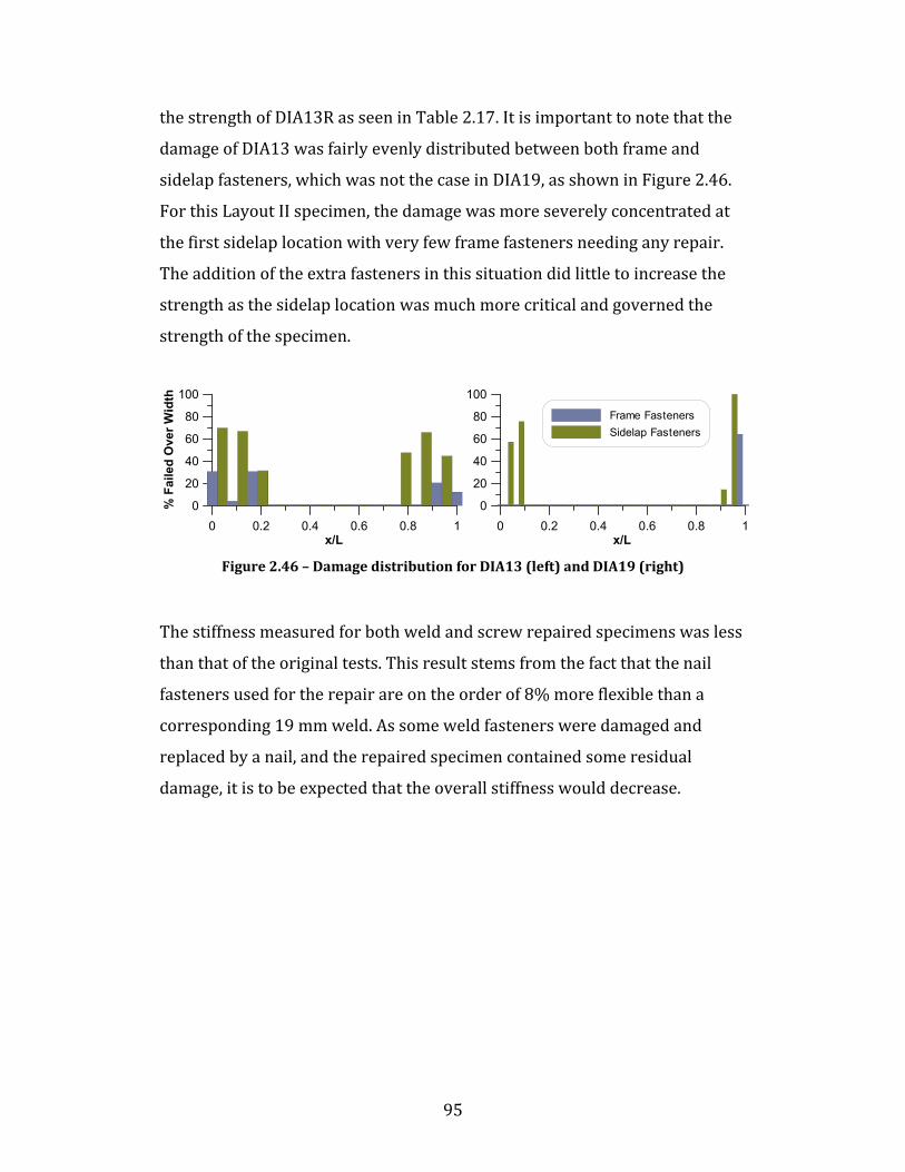
95

the strength of DIA13R as seen in Table 2.17. It is important to note that the damage of DIA13 was fairly evenly distributed between both frame and sidelap fasteners, which was not the case in DIA19, as shown in Figure 2.46. For this Layout II specimen, the damage was more severely concentrated at the first sidelap location with very few frame fasteners needing any repair. The addition of the extra fasteners in this situation did little to increase the strength as the sidelap location was much more critical and governed the strength of the specimen.

Figure 2.46 – Damage distribution for DIA13 (left) and DIA19 (right) The stiffness measured for both weld and screw repaired specimens was less than that of the original tests. This result stems from the fact that the nail fasteners used for the repair are on the order of 8% more flexible than a corresponding 19 mm weld. As some weld fasteners were damaged and replaced by a nail, and the repaired specimen contained some residual damage, it is to be expected that the overall stiffness would decrease.

0 0.2 0.4 0.6 0.8 1x/L

0

20

40

60

80

100

0 0.2 0.4 0.6 0.8 1x/L

0

20

40

60

80

100

% F

aile

d O

ver W

idth

Frame FastenersSidelap Fasteners

96

Chapter 3 - STRUCTURAL DESIGN AND MODELLING

3.1 Overview of Task Single-storey buildings are typically laterally supported by vertical bracing members found in either the exterior or interior bays of a structure. The NBCC 2005 (NRCC, 2005) recognizes two primary forms of lateral bracing systems to be used in the seismic force resisting system. These are: concentrically braced frames (CBF), in which the lateral braces act as the fuse element, and eccentrically braced frames (EBF), where a portion of the beam to which the braces are attached, known as the link, is able to dissipate energy by yielding in shear or flexure. The design procedure for a single storey structure with an EBF is presented in this chapter using three different assumptions of diaphragm shear stiffness: rigid, diaphragm with the SDI (Luttrell, 2004) predicted stiffness, and 70% of the SDI stiffness which represents an average of the stiffness values under dynamic excitation from the diaphragm tests presented in this thesis. Furthermore, the design was completed for each of the stiffness assumptions using various upper limits of the fundamental period for the calculation of the seismic design forces, namely 2Ta, 2.5Ta, 3Ta and an unbounded period. 3.2 Building Location and Geometry The structure being studied was chosen to be located in Abbotsford, BC, a western Canadian city which is found in a zone of high seismicity and heavy snowfall. A site class of C, with very dense soil and soft rock was also selected such that the acceleration-based and velocity-based site coefficients were equal to unity. The design spectrum values are represented in Figure 3.1.

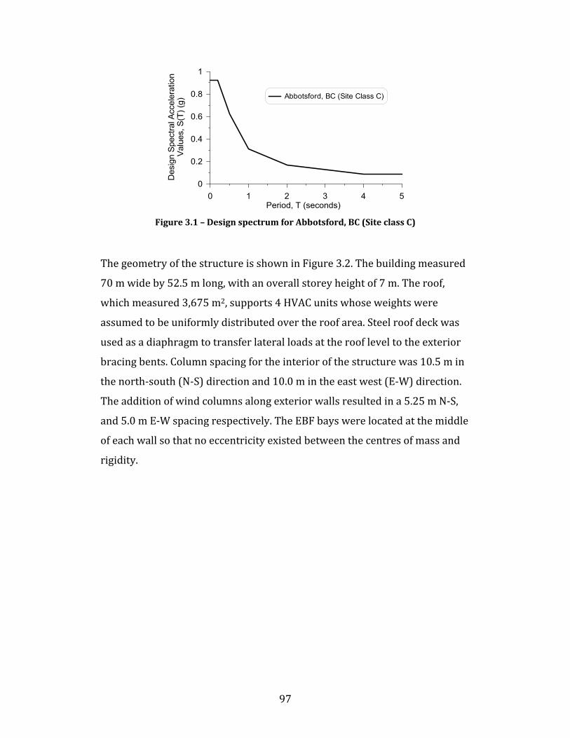
97

Figure 3.1 – Design spectrum for Abbotsford, BC (Site class C) The geometry of the structure is shown in Figure 3.2. The building measured 70 m wide by 52.5 m long, with an overall storey height of 7 m. The roof, which measured 3,675 m2, supports 4 HVAC units whose weights were assumed to be uniformly distributed over the roof area. Steel roof deck was used as a diaphragm to transfer lateral loads at the roof level to the exterior bracing bents. Column spacing for the interior of the structure was 10.5 m in the north-south (N-S) direction and 10.0 m in the east west (E-W) direction. The addition of wind columns along exterior walls resulted in a 5.25 m N-S, and 5.0 m E-W spacing respectively. The EBF bays were located at the middle of each wall so that no eccentricity existed between the centres of mass and rigidity.

0 1 2 3 4 5Period, T (seconds)

0

0.2

0.4

0.6

0.8

1

Des

ign

Spe

ctra

l Acc

eler

atio

nV

alue

s, S

(T) (

g)

Abbotsford, BC (Site Class C)

98

Figure 3.2 – Roof plan and wall elevation of single-storey building

3.3 Design Loads A structure is to be designed to have sufficient capacity and integrity to resist all loads that can be expected over its service life. For this purpose, the NBCC (NRCC, 2005) has set governing combinations that designers should use when considering the loads affecting individual members. For example, the governing load case for the seismic force resisting system is based on the combination of 1.0D + 1.0E + 0.5L + 0.25S, where D, E, L and S represent the dead, earthquake, live and snow loads respectively. This load case, however, does not govern the design of the gravity resisting members in the roof where the combination of 1.25D + 1.5S + 0.5L was found to be critical. It is by evaluating a series of load combinations for individual members that the worst effects can be properly designed for. A breakdown of the loads for the structure in study follows.

99

3.3.1 Dead and Live Loads The dead load applied to the structure included the weight of roofing components and the exterior cladding. At the roof level, the following elements contributed to the dead load: HVAC units, lighting, fans and sprinkler systems (0.10 kPa), walkways, roof ballast, membrane, insulation and joists (1.00 kPa) and steel roof deck (0.10 kPa). The total roof load from the sum of these components was 1.20 kPa. The exterior walls were composed of an insulated metal wall system with interior and exterior metal sheeting. The estimated weight of such a system was 0.35 kPa. The only live loads applied were at the roof level, where a use and occupancy load of 1.0 kPa was specified as per the NBCC 2005 (NRCC, 2005). 3.3.2 Snow Loads Snow loads were determined according to Cl. 4.1.6 of the NBCC 2005. The basic snow load equation is shown in Equation 3.1. S I S C C C C S (3.1) S Specified snow load (kPa)S , S 1-in-50 year ground snow load and associated rain load, 2.0, 0.3 (kPa)I Importance factor for snow load, 1.0C Basic roof snow load factor, 0.8C Wind exposure factor, 1.0C Roof slope factor, 1.0C Roof shape factor, 1.0 Accumulation of snow in the vicinity of the HVAC units was also taken into account and assumed uniformly distributed over the entire roof area. This increased the basic snow load from a value of 1.90 kPa to 1.96 kPa.

100

3.3.3 Wind Loads Similarly to snow loads, wind loads were determined using Cl. 4.1.7 of the NBCC 2005. The wind was considered acting in both the N-S and E-W directions independently in order to determine the maximum loading effects on structural members in both lateral directions. The basic wind load equation is shown in Equation 3.2 (3.2) Specified external pressure acting normal to the surface (kPa) Importance factor for wind, 1.0 Reference velocity pressure, 0.62 kPa Exposure factor, 0.93 Gust effect factor, varied External pressure coefficient, varied When calculating the wind loads, the NBCC considers an end portion of the wall surface normal to the wind direction to be of higher pressure than the remainder of the wall. In the structure under study, these higher pressure zones resulted in wind pressures of 0.66 kPa and -0.46 kPa on the windward and leeward walls. The corresponding pressures for the low pressure zone were 0.43 kPa and -0.32 kPa respectively. 3.3.4 Seismic Loads An overview of determining the seismic forces acting on a structure was provided in Section 1.6.1. A more detailed explanation of this method as it relates to the building of study is now presented. Seismic forces were obtained using the equivalent static force procedure described in the NBCC 2005 Cl. 4.1.8. The magnitude of the seismic base shear was calculated from Equations 3.3 and 3.4. The seismic weight was determined using 100% of the dead load from roofing materials, 50% (upper

101

half) of cladding on the walls, and 25% of the roof snow load including accumulation effects. It was assumed for the calculations that the structure was of normal importance. (3.3) Minimum lateral earthquake load force (kN) Spectral acceleration values at the fundamental lateral period A factor to account for the effect of higher modes, 1.0 Importance factor of the structure, 1.0 Seismic weight of the building, 6508.9 kN Ductility-related force modification factor, 4.0 Overstrength-related force modification factor, 1.5 Where V is bounded by the following limits: 2.0 23 0.2 (3.4) The fundamental period of the structure, Ta = 0.175 seconds, was first calculated using Equation 3.5. The NBCC currently allows for a longer period to be used for the equivalent static force calculations, up to a limit of 2Ta, if it can be shown from elastic dynamic analysis that the actual fundamental period of the structure is longer than the 2Ta limit. It was therefore decided to start the seismic design of the structure using period assumptions corresponding to 2Ta, 2.5Ta, 3Ta and 2Ta for each of the four upper bound limit scenarios of the fundamental period that would have to be verified by a model of the structure created in SAP2000 (CSI, 2010). The selection of the initial values was done to correspond to the uppermost limit of Ta, while the value of 2Ta for the case in which the period was allowed to increase unbounded was arbitrarily chosen as a starting point. Spectral acceleration

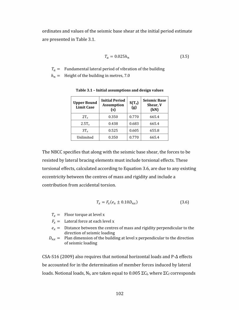
102

ordinates and values of the seismic base shear at the initial period estimate are presented in Table 3.1. 0.025 (3.5) Fundamental lateral period of vibration of the building Height of the building in metres, 7.0 Table 3.1 – Initial assumptions and design values

Upper BoundLimit Case

Initial PeriodAssumption

(s)

S(Ta)(g)

Seismic BaseShear, V

(kN) 2Ta 0.350 0.770 665.4 2.5Ta 0.438 0.683 665.4 3Ta 0.525 0.605 655.8 Unlimited 0.350 0.770 665.4 The NBCC specifies that along with the seismic base shear, the forces to be resisted by lateral bracing elements must include torsional effects. These torsional effects, calculated according to Equation 3.6, are due to any existing eccentricity between the centres of mass and rigidity and include a contribution from accidental torsion. 0.10 (3.6) Floor torque at level x Lateral force at each level x Distance between the centres of mass and rigidity perpendicular to the direction of seismic loading Plan dimension of the building at level x perpendicular to the direction of seismic loading CSA-S16 (2009) also requires that notional horizontal loads and P-Δ effects be accounted for in the determination of member forces induced by lateral loads. Notional loads, Nf, are taken equal to 0.005 ΣCf, where ΣCf corresponds

103

to the total gravity load carried by the building columns (ΣCf = 6209 kN, Nf = 31.0 kN). P-Δ effects are accounted for by multiplying the effects of lateral loads, including notional loads, by the factor U2, given by Equation 3.7. 1 ∑ ∆∑ (3.7) Amplification factor to account for second-order effects Total gravity load carried by columns Ductility-related force modification factor∆ First-order displacement of the structure due to factored loads Factored shear force on the structure Height of the structure At the preliminary design stage, the storey drift, Δ, is unknown and was assumed equal to 0.006h, which resulted in U2 = 1.06. The stiffness of the roof diaphragm is not yet known either and so simple assumptions were made to come up with the preliminary design values. For the case where the diaphragm was considered infinitely rigid, the lateral stiffness of the braced frames was assumed to be equal for all braced bays, leading to 59% and 55% of the lateral force, including accidental torsional moments, being resisted by each braced frame in the N-S and E-W directions respectively. For the flexible diaphragm case, it was assumed that only the two braced bays in the direction of motion resisted the lateral force, which led to 60% of the lateral load being resisted by any of the braced frames when including in-plane accidental torsion. The governing forces to be resisted by the braced frames for all three diaphragm stiffness assumptions and all four upper bound limits on the fundamental period are provided in Table 3.2.

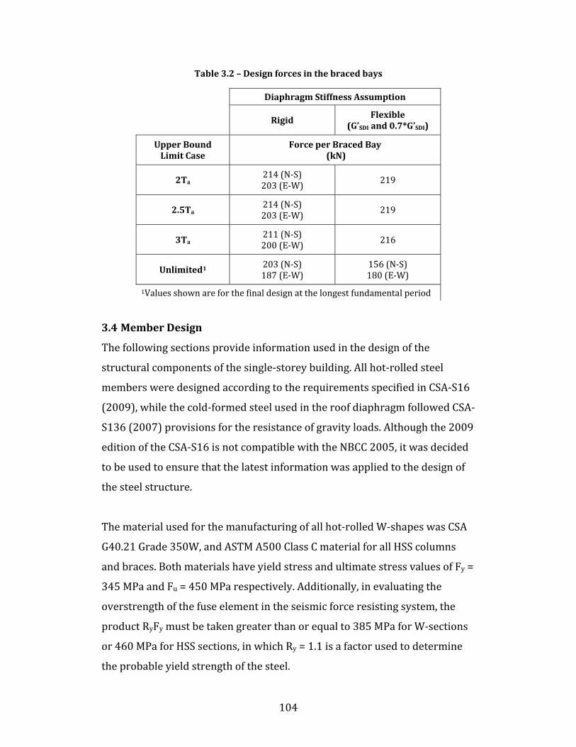
104

Table 3.2 – Design forces in the braced bays

Diaphragm Stiffness Assumption

Rigid Flexible (G’SDI and 0.7*G’SDI)

Upper Bound Limit Case Force per Braced Bay

(kN)

2Ta 214 (N-S) 203 (E-W) 219

2.5Ta 214 (N-S) 203 (E-W) 219 3Ta

211 (N-S) 200 (E-W) 216 Unlimited1

203 (N-S) 187 (E-W) 156 (N-S) 180 (E-W) 1Values shown are for the final design at the longest fundamental period 3.4 Member Design The following sections provide information used in the design of the structural components of the single-storey building. All hot-rolled steel members were designed according to the requirements specified in CSA-S16 (2009), while the cold-formed steel used in the roof diaphragm followed CSA-S136 (2007) provisions for the resistance of gravity loads. Although the 2009 edition of the CSA-S16 is not compatible with the NBCC 2005, it was decided to be used to ensure that the latest information was applied to the design of the steel structure. The material used for the manufacturing of all hot-rolled W-shapes was CSA G40.21 Grade 350W, and ASTM A500 Class C material for all HSS columns and braces. Both materials have yield stress and ultimate stress values of Fy = 345 MPa and Fu = 450 MPa respectively. Additionally, in evaluating the overstrength of the fuse element in the seismic force resisting system, the product RyFy must be taken greater than or equal to 385 MPa for W-sections or 460 MPa for HSS sections, in which Ry = 1.1 is a factor used to determine the probable yield strength of the steel.

105

3.4.1 Seismic Force Resisting System The size of the link element in the EBF frame is initially selected to be able to adequately resist the shear forces induced by seismic ground motions. The required shear area, calculated using Equation 3.8 is then determined so that an appropriate Class 1 section may be chosen. During this step, it is crucial to try and select a beam section that only just satisfies the required shear area as the overstrength of the system is directly related to this parameter. ,0.55φ (3.8) Required shear area of link section, Factored shear force to be resisted by link φ Resistance factor, 0.9 Yield strength of steel Once a size is selected, the required length of the link can be found such that the desired inelastic behaviour, yielding in shear for the case of the structure under study, will occur. A link that yields only in shear is obtained by specifying the link length, e, such that Equation 3.9 is satisfied. 1.6 (3.9) Maximum length of the link element for yielding in shear Plastic moment capacity of the link section (ZxFy) Plastic shear capacity of the link section (0.55dwFy) Additionally, it is important to limit the total rotation of the link relative to the rest of the beam, γ, represented in Figure 3.3 by providing a link length that satisfies Equation 3.10. Additional requirements for the link length, as specified in CSA S16 (2009) must also be considered.

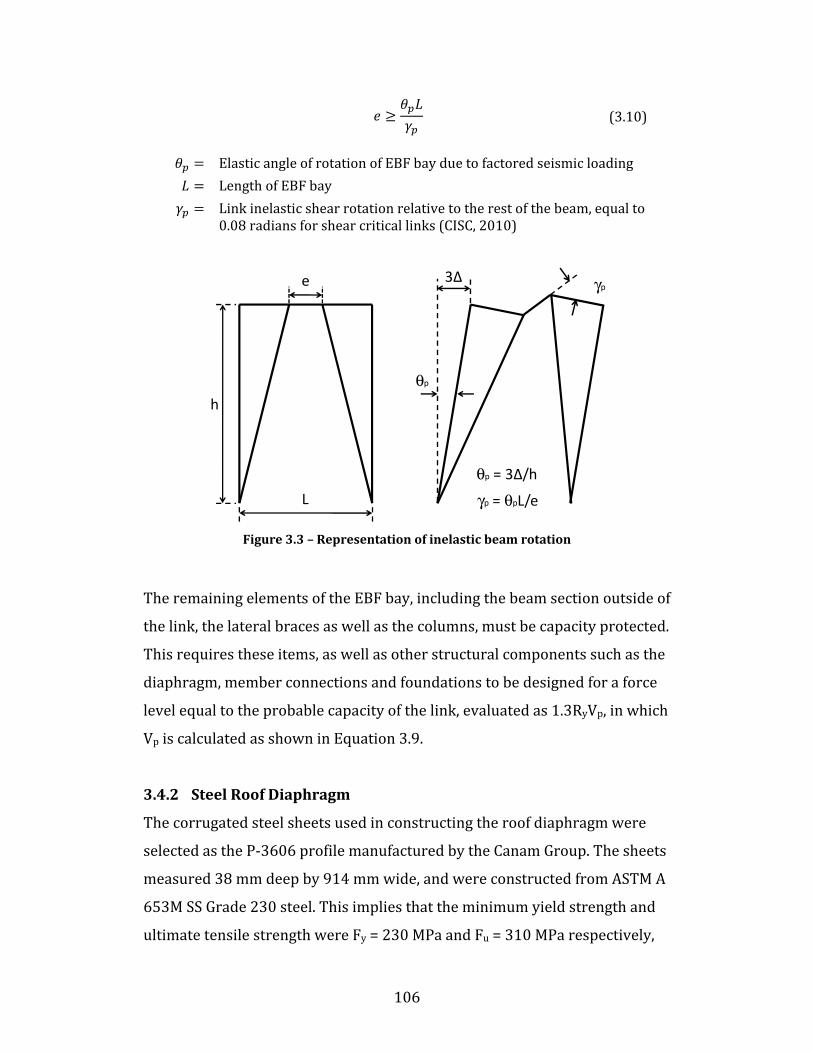
106

(3.10) Elastic angle of rotation of EBF bay due to factored seismic loading Length of EBF bay Link inelastic shear rotation relative to the rest of the beam, equal to 0.08 radians for shear critical links (CISC, 2010)

Figure 3.3 – Representation of inelastic beam rotation The remaining elements of the EBF bay, including the beam section outside of the link, the lateral braces as well as the columns, must be capacity protected. This requires these items, as well as other structural components such as the diaphragm, member connections and foundations to be designed for a force level equal to the probable capacity of the link, evaluated as 1.3RyVp, in which Vp is calculated as shown in Equation 3.9.

3.4.2 Steel Roof Diaphragm The corrugated steel sheets used in constructing the roof diaphragm were selected as the P-3606 profile manufactured by the Canam Group. The sheets measured 38 mm deep by 914 mm wide, and were constructed from ASTM A 653M SS Grade 230 steel. This implies that the minimum yield strength and ultimate tensile strength were Fy = 230 MPa and Fu = 310 MPa respectively,

θp

γp = θpL/e

θp = 3Δ/h

L

e

h

γp3Δ

107

with a modulus of elasticity of E = 203,000 MPa. Diaphragm action was obtained by fastening the steel sheets to the underlying frame and to each other using Hilti X-EDNK19 and X-EDNK22 power-actuated frame fasteners and #12 self-tapping sidelap screws. Based on gravity loading alone, the minimum sheet steel thickness was determined to be 0.91 mm. The SDI methodology, as discussed in Section 1.6.2.1 was used to obtain the ultimate in-plane shear strength and stiffness of the diaphragms. For the calculations, the deck sheets were assumed to be of 10 m total length spanning over open web steel joists spaced at 2.0 m o/c. A resistance factor of φ = 0.6 was used to determine the factored in-plane shear strength of the diaphragm assemblies as recommended by CSA S136 (2007) for mechanical fasteners. With regards to seismic design, the diaphragm must be designed to remain elastic given the probable force developed in the EBF link. This force is represented by Equation 3.11 assuming one braced bay per wall. 2 1 (3.11) Factored in-plane shear force to be resisted by the diaphragm Probable shear capacity of the link, equal to 1.3RyVp Angle of the braces measured from a horizontal plane Length of EBF bay Length of link Width of the diaphragm

3.4.3 Gravity Resisting Members The roof structure in the east-west direction was constructed using a Gerber system in which the beams are cantilevered over interior columns in order to reduce the maximum bending moments for design. The cantilever length was

108

selected as 12% of the interior bay spacing of 10 m, resulting in a 1.2 m overhang. Link beams, or drop-in beams were used to span the remaining distance. Along the exterior walls of the structure, eave beams were designed assuming a simply-supported 10 m span. Additional seismic loads inducing compression and tension forces in these perimeter members also needed to be combined with gravity loading for their final design. Roof framing in the N-S direction consisted of 10.5 m long open web steel joists (OWSJ) spaced at 2.0 m o/c. Interior columns were designed to resist the force combination of 1.25D + 1.5S + 0.5L at the roof level acting over a tributary area of 105 m2. The members, selected as square HSS sections, were assumed pin-ended at both ends. 3.4.4 Wind Resisting Members Columns along the exterior walls of the structure were selected as I-shaped members with wind loads inducing bending about their strong axis. Wind columns were assumed to take no gravity load and resisted only the effects due to wind, while exterior columns were designed for both wind and gravity loading. Corner columns located at the intersection of the exterior walls were designed for bi-axial bending as well as for gravity. Girts, spaced at 1.75 m o/c were assumed over the height of the walls in order to allow for attachment of the cladding and to reduce the unbraced length of the columns in their weak axis. Additional moments due to eccentricities from the beam connection at the top of the column were also included. A summary of the shapes and sizes of the structural components which largely remained unchanged during the various diaphragm design and period upper bound assumptions is provided in Table 3.3.

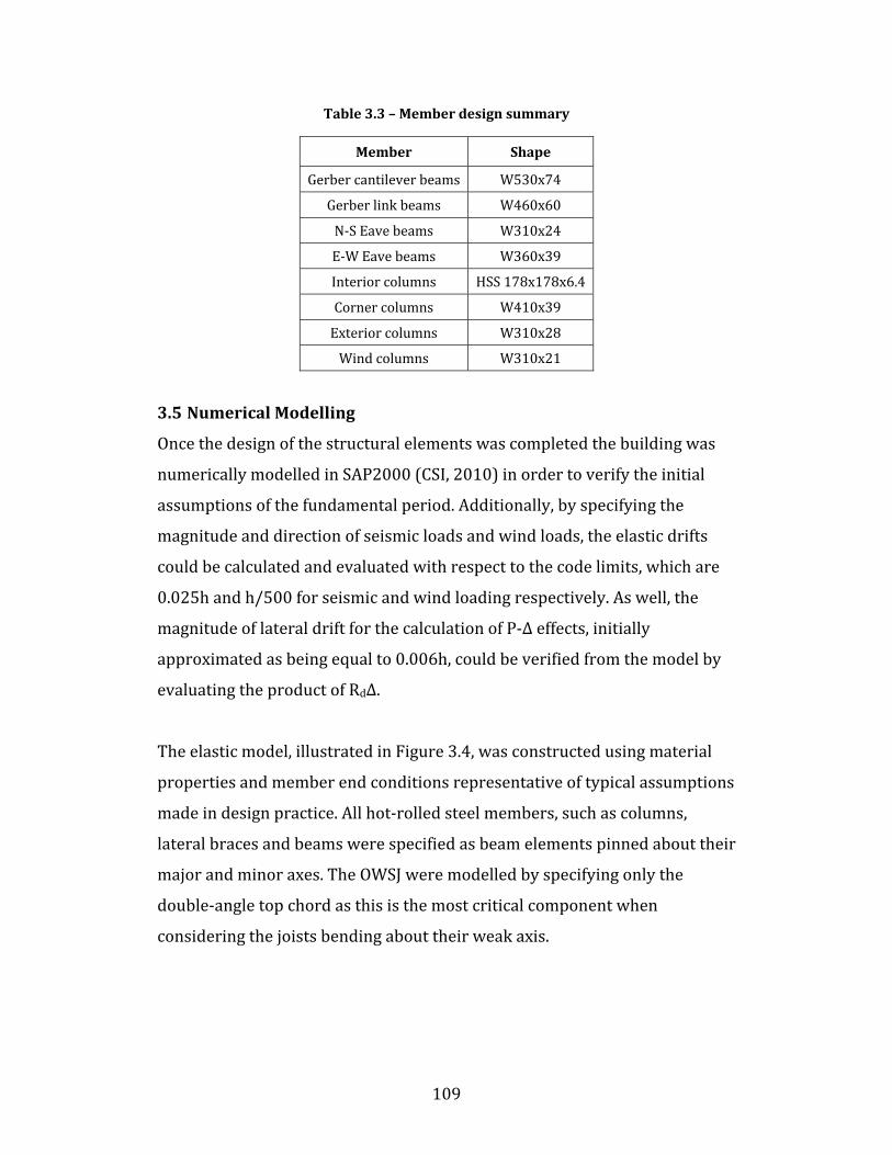
109

Table 3.3 – Member design summary

Member Shape Gerber cantilever beams W530x74 Gerber link beams W460x60 N-S Eave beams W310x24 E-W Eave beams W360x39 Interior columns HSS 178x178x6.4Corner columns W410x39 Exterior columns W310x28 Wind columns W310x21 3.5 Numerical Modelling Once the design of the structural elements was completed the building was numerically modelled in SAP2000 (CSI, 2010) in order to verify the initial assumptions of the fundamental period. Additionally, by specifying the magnitude and direction of seismic loads and wind loads, the elastic drifts could be calculated and evaluated with respect to the code limits, which are 0.025h and h/500 for seismic and wind loading respectively. As well, the magnitude of lateral drift for the calculation of P-Δ effects, initially approximated as being equal to 0.006h, could be verified from the model by evaluating the product of RdΔ. The elastic model, illustrated in Figure 3.4, was constructed using material properties and member end conditions representative of typical assumptions made in design practice. All hot-rolled steel members, such as columns, lateral braces and beams were specified as beam elements pinned about their major and minor axes. The OWSJ were modelled by specifying only the double-angle top chord as this is the most critical component when considering the joists bending about their weak axis.

110

Figure 3.4 – 3D model of the structure The roof diaphragm was constructed using 2.0 m wide by 2.5 m long four-node shell elements. The plane elements were assigned a thickness of 0.91 mm, equal to the actual sheet thickness of the diaphragm. SAP2000 allows for modification factors to be applied to the shell element properties independently. It was thus possible to account for the diaphragm in-plane shear stiffness, G’, as calculated by the SDI procedure (Luttrell, 2004) where the shear stiffness modifier was calculated according to Equation 3.12. This was done as the stiffness of a corrugated deck sheet is less than that of a flat plate of the same thickness. For the design involving a fully rigid system, diaphragm constraints were added to the model in the plane of the roof area, causing all affected joints to move together as a planar diaphragm fully rigid against any in-plane shear deformations. For the purpose of constraining both directions of movement, a diaphragm constraint needed to be created for both the N-S and E-W directions of movement respectively.

Shear stiffness modifier (3.12) In-plane shear stiffness obtained from the SDI procedure Shear modulus of cold-formed steel Diaphragm sheet steel thickness

111

Additionally, to account for the seismic mass acting at the roof level, the mass modifier of the shell elements used to reproduce the roof diaphragm was altered following Equation 3.13. Lumped masses were also added to the joints located at the tops of the walls to represent the mass of cladding components distributed around the perimeter of the structure. Mass modifier (3.13) Factored seismic weight on the roof determined from 1.0D+0.25S Weight per unit volume of cold-formed steel Diaphragm sheet steel thickness 3.6 Design Summary and Findings The following sections present an overview of the findings from the design of the structure for each of the three different diaphragm stiffness assumptions: fully rigid, SDI stiffness (Luttrell, 2004), and 70% of the SDI stiffness, and the four upper limits of the fundamental period for the calculation of the seismic design forces: 2Ta, 2.5Ta, 3Ta and unlimited. The primary goal of this study was to design the structure under the various stiffness assumptions while minimizing the thickness and number of fasteners used in the construction of the roof diaphragm, as even slight increases in either of these two variables involves relatively costly upgrades due to the large surface area of the roof and the number of frame and sidelap fasteners required. For each of the stiffness and fundamental period assumptions, multiple attempts were made at designing the structure in order to achieve the most economical diaphragm design.

112

3.6.1 Fully Rigid System The structure with a fully rigid roof diaphragm was braced laterally using a single EBF bay per wall. The bay width, equal to the spacing of the wind columns, measured 5.25 m in the N-S direction and 5.0 m in the E-W. This narrow arrangement required a relatively large member to be selected as the link beam; however it also allowed for a shorter link length, e, to be specified thereby limiting the moment to be resisted by the beam section outside of the link. Furthermore, due to the steep angle of the braces with respect to the horizontal, the majority of the probable force developed by the link was transferred as a vertical compression force through the braces as opposed to a horizontal compression in the beam member outside of the link, reducing the design force of the roof diaphragm. Finally, because of the rigid diaphragm constraints applied at the roof level, all drift assumptions used to calculate the P-Δ effects, as well as the maximum amplified seismic drifts were easily satisfied. The assumption that the fundamental period of the structure was greater than 2Ta was also verified to be correct. A summary of the design can be found in Table 3.4. An alternative design was also attempted by removing a wind column and expanding the EBF bay to 10.5 m and 10.0 m in the N-S and E-W directions respectively. Using this method, the shear force to be resisted by the link beam was significantly reduced, to 275 kN from 572 kN in the previous method, due to the change in bay geometry. However, even though a smaller link shape was used to resist the decreased forces, which in turn reduced the probable capacity at yield, the compression force on the beam outside of the link was significantly higher because of the angle of the braces. This had the undesired effect of increasing the force to be resisted by the roof diaphragm, despite being able to select a smaller section for both the beam and the lateral braces in the EBF system.

113

For the case of the rigid roof diaphragm, allowing the fundamental period for the determination of the seismic design forces to elongate to 2.5Ta did not have any effect on the design of the structure. This is because the seismic forces were not governed by the fundamental period but by the specified NBCC maximum represented by the right side of Equation 3.4. The seismic forces were therefore the same at the 2Ta and 2.5Ta levels for the structure under study. Allowing the fundamental period to elongate to the 3Ta level changed the governing seismic force equation to Equation 3.3. This value, however, was essentially equal to the upper limit maximum used for the 2Ta and 2.5Ta cases resulting in the same design as shown in Table 3.4. The design of the structure with an unlimited period for the calculation of the seismic forces was done in an iterative manner. Initially, a period equal to 2Ta was selected as a starting point and the structure was designed for the forces shown in Table 3.1. From the SAP2000 model, the fundamental period in both directions was then obtained and subsequently used in order to recalculate the seismic forces and redesign the building under the actual period. This procedure was repeated until the change in period from one iteration to the next became small enough that the new forces in the structure did not result in a change in the member sizes and the design of the building remained the same. Allowing the period to elongate unbounded resulted in a 5% decrease in the magnitude of the seismic forces for the rigid diaphragm case. The structure was therefore able to be designed using a link section of smaller cross-sectional area which decreased the demand on the roof diaphragm and allowed for this element to be connected using fewer fasteners. The drift limitations were also easily satisfied due to the assumed fully rigid roof diaphragm. The final design is shown in Table 3.5.

114

3.6.2 Diaphragm with SDI Stiffness The initial strategy for the design of the structure with a flexible roof diaphragm was to keep the smaller EBF bay geometry from the fully rigid case. However, after analysis of the model, it was determined that this more narrow and flexible EBF arrangement, along with the increased diaphragm flexibility, increased the drift values towards the allowable NBCC maximum. It was therefore decided to increase the bay width to the larger size mentioned in Section 3.6.1 in order to increase the stiffness of the structure and help in limiting the total lateral drift. The central wind column in both the N-S and E-W directions was therefore removed to expand the central bays to 10.5 m and 10.0 m in the N-S and E-W directions respectively. The result of the more horizontal alignment of the lateral braces was that an additional 0.7 kN/m of shear force had to be resisted by the roof diaphragm, which resulted in one additional screw per sidelap. The new geometry also allowed for a smaller link beam and lateral brace size to be specified, as well as four fewer columns which were removed to accommodate the wider EBF bay geometry. Similar to the rigid diaphragm case, allowing the fundamental period to increase to values of 2.5Ta and 3Ta had no significant impact on the design as the seismic forces saw little or no decrease for this particular structure. A summary of the design for the flexible diaphragm structure is presented in Table 3.6. As for the fully rigid system, the design for the single-storey structure with an unbounded period for the seismic force calculations was done in an iterative manner with an initial period estimate of 2Ta. The design was also performed using the wider bay spacing of 10.5 m and 10.0 m in the N-S and E-W directions respectively in order to limit lateral drift.

115

At the final design stage, it was found that a drop in the seismic forces on the order of 29% for the N-S direction, and 18% for the E-W direction was obtained using this method. This reduction allowed for link sections of smaller cross-sectional area to be selected as the energy-dissipating element, reducing the impact on both the lateral braces and number of fasteners required in the roof diaphragm. Drift limitations at the final design were satisfied, however the initial assumption of RdΔ = 0.006h used in Equation 3.7 for the calculation of U2, an amplification factor that accounts for P-Δ effects, was surpassed in the N-S direction. As the minimum link length, e, as calculated by Equation 3.10 is directly related to the magnitude of the drift, an increase in link length from 600 mm to 650 mm was required in this direction. The final design is summarized in Table 3.7. 3.6.3 Diaphragm with 70% of SDI Stiffness The techniques used for the design of the structure with a flexible roof diaphragm, in which a stiffness of 0.7*G’SDI as determined from the large-scale experiments was used, were similar to those presented in Section 3.6.2 except that the effects of drift were even more pronounced. To mitigate this effect, the wider EBF bay spacing was used in both orthogonal directions. Allowing for the fundamental period of the structure to increase in the determination of the seismic forces had no effect as again, the right side of Equation 3.4 governed for both the 2Ta and 2.5Ta case. For an upper limit of 3Ta, the governing clause was changed to Equation 3.3, but the value as determined using this formula resulted in essentially no increase in the magnitude of the lateral seismic force. A summary of the designs can be found in Table 3.8. When allowing the fundamental period to increase unbounded for the determination of the seismic design forces, a drop in magnitude of 37% and 26% in the N-S and E-W directions was experienced. As a result, the link

116

beam could be designed using a smaller member size which positively affected the in-plane shear forces to be resisted by the roof diaphragm. After the third design iteration, it was found that the increase in fundamental period in both directions did not result in any changes in the member sizes and hence had no further impact on the design of the diaphragm. Much like the case presented in Section 3.6.2, where the full SDI stiffness was used along with an unbounded period, the RdΔ = 0.006h assumption was surpassed and necessitated an increase in the link segment from 600 mm to 675 mm in the more critical N-S direction. This change resulted in a slightly more flexible structure, decreasing the seismic forces to their final value. The final design is presented in Table 3.9.

117

Table 3.4 – Design summary with rigid roof diaphragm (2Ta, 2.5Ta and 3Ta)

Property

Diaphragm Stiffness Assumption: Rigid

N-S Direction E-W Direction Rd, Ro 4.0, 1.5 Ta (s) 0.175 Tdesign (s) 0.350 (2Ta), 0.438 (2.5Ta), 0.525 (3Ta) Link Member Design Vf (kN) 572 568 Link Shape W460x52 elink (mm) 450 V’p (kN) 649 EBF Member Design Cbrace (kN) 1044 1107 Brace Shape HSS 254x254x8.0 Ccolumn (kN) 157 159 Column Shape W310x28 Roof Diaphragm Design qf (kN/m) 12.9 t (mm) 0.91 Fastener Pattern 36/7 Sidelap Spacing (mm) 220 Sn (kN/m) 21.5 G’SDI (kN/mm) 21.6 Fundamental Period Tactual (s) 0.549 0.575 Deflection Under Seismic Load ΔE (mm) 6.9 7.8 RdRoΔE (mm) 41.6 47.0 0.025h (mm) 175.0 175.0 Deflection Under Wind Load ΔW (mm) 2.2 1.8 h/500 (mm) 14.0 14.0

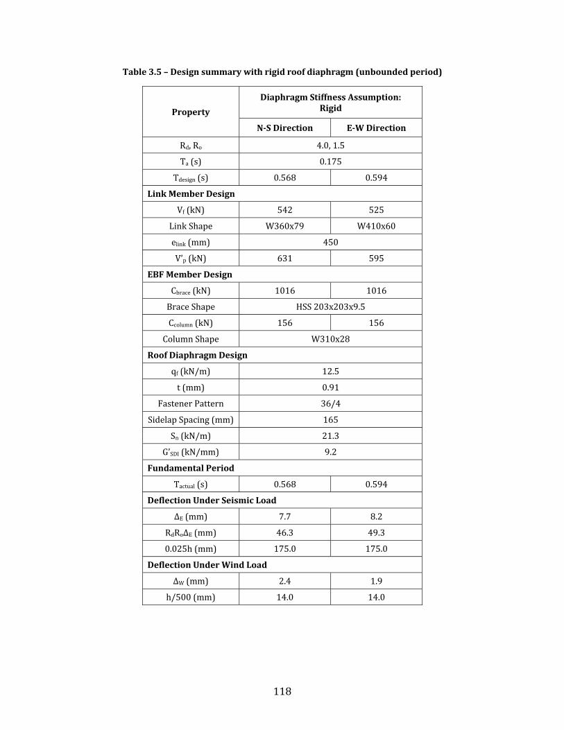
118

Table 3.5 – Design summary with rigid roof diaphragm (unbounded period)

Property

Diaphragm Stiffness Assumption: Rigid

N-S Direction E-W Direction Rd, Ro 4.0, 1.5 Ta (s) 0.175 Tdesign (s) 0.568 0.594 Link Member Design Vf (kN) 542 525 Link Shape W360x79 W410x60 elink (mm) 450 V’p (kN) 631 595 EBF Member Design Cbrace (kN) 1016 1016 Brace Shape HSS 203x203x9.5 Ccolumn (kN) 156 156 Column Shape W310x28 Roof Diaphragm Design qf (kN/m) 12.5 t (mm) 0.91 Fastener Pattern 36/4 Sidelap Spacing (mm) 165 Sn (kN/m) 21.3 G’SDI (kN/mm) 9.2 Fundamental Period Tactual (s) 0.568 0.594 Deflection Under Seismic Load ΔE (mm) 7.7 8.2 RdRoΔE (mm) 46.3 49.3 0.025h (mm) 175.0 175.0 Deflection Under Wind Load ΔW (mm) 2.4 1.9 h/500 (mm) 14.0 14.0

119

Table 3.6 – Design summary with flexible roof diaphragm (G’SDI) (2Ta, 2.5Ta and 3Ta)

Property

Diaphragm Stiffness Assumption: Flexible (G’SDI)

N-S Direction E-W Direction Rd, Ro 4.0, 1.5 Ta (s) 0.175 Tdesign (s) 0.350 (2Ta), 0.438 (2.5Ta), 0.525 (3Ta) Link Member Design Vf (kN) 292 307 Link Shape W250x39 W310x39 elink (mm) 600 600 V’p (kN) 328 341 EBF Member Design Cbrace (kN) 627 676 Brace Shape HSS 203x203x8.0 Ccolumn (kN) 144 147 Column Shape W310x28 Roof Diaphragm Design qf (kN/m) 13.6 t (mm) 0.91 Fastener Pattern 36/7 Sidelap Spacing (mm) 200 Sn (kN/m) 23.0 G’SDI (kN/mm) 22.4 Fundamental Period Tactual (s) 0.730 0.651

Deflection Under Seismic Load ΔE (mm) 12.5 10.4 RdRoΔE (mm) 74.7 62.3 0.025h (mm) 175.0 175.0 Deflection Under Wind Load ΔW (mm) 4.8 2.5 h/500 (mm) 14.0 14.0

120

Table 3.7 – Design summary with flexible roof diaphragm (G’SDI) (unbounded period)

Property

Diaphragm Stiffness Assumption: Flexible (G’SDI)

N-S Direction E-W Direction Rd, Ro 4.0, 1.5 Ta (s) 0.175 Tdesign (s) 0.828 0.704 Link Member Design Vf (kN) 208 252 Link Shape W200x42 W200x52 elink (mm) 650 600 V’p (kN) 280 309 EBF Member Design Cbrace (kN) 538 616 Brace Shape HSS 203x203x6.4 HSS 203x203x8.0 Ccolumn (kN) 142 144 Column Shape W310x28 Roof Diaphragm Design qf (kN/m) 12.2 t (mm) 0.91 Fastener Pattern 36/7 Sidelap Spacing (mm) 225 Sn (kN/m) 21.5 G’SDI (kN/mm) 21.6 Fundamental Period Tactual (s) 0.828 0.704

Deflection Under Seismic Load ΔE (mm) 13.5 11.2 RdRoΔE (mm) 80.9 67.1 0.025h (mm) 175.0 175.0 Deflection Under Wind Load ΔW (mm) 5.7 2.9 h/500 (mm) 14.0 14.0

121

Table 3.8 – Design summary with flexible roof diaphragm (0.7*G’SDI) (2Ta, 2.5Ta and 3Ta)

Property

Diaphragm Stiffness Assumption: Flexible (0.7*G’SDI)

N-S Direction E-W Direction Rd, Ro 4.0, 1.5 Ta (s) 0.175 Tdesign (s) 0.350 (2Ta), 0.438 (2.5Ta), 0.525 (3Ta) Link Member Design Vf (kN) 292 307 Link Shape W250x39 W310x39 elink (mm) 600 600 V’p (kN) 328 341 EBF Member Design Cbrace (kN) 627 676 Brace Shape HSS 203x203x8.0 HSS 203x203x8.0 Ccolumn (kN) 144 147 Column Shape W310x28 Roof Diaphragm Design qf (kN/m) 13.6 t (mm) 0.91 Fastener Pattern 36/7 Sidelap Spacing (mm) 200 Sn (kN/m) 23.0 G’SDI (kN/mm) 22.4 Fundamental Period Tactual (s) 0.774 0.678 Deflection Under Seismic Load ΔE (mm) 13.4 11.1 RdRoΔE (mm) 80.3 66.7 0.025h (mm) 175.0 175.0 Deflection Under Wind Load ΔW (mm) 5.4 2.8 h/500 (mm) 14.0 14.0

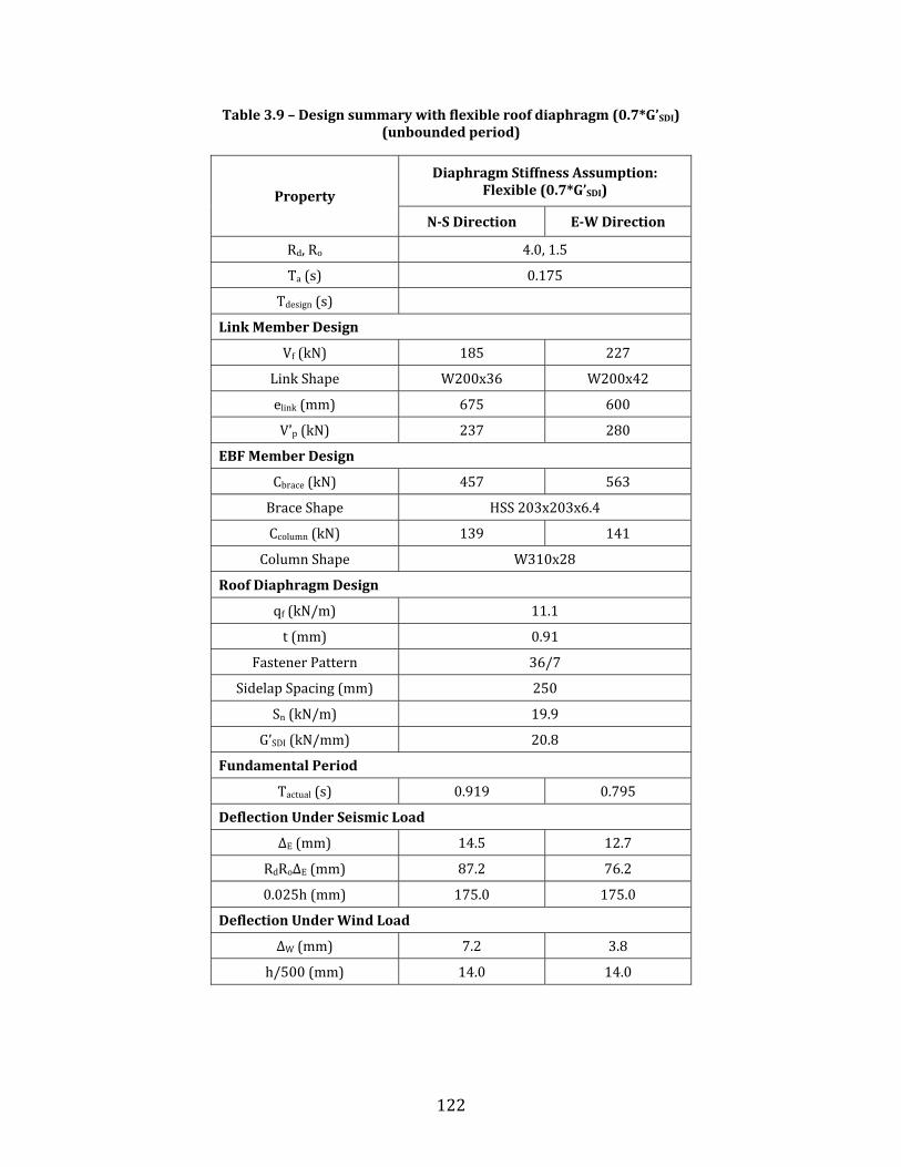
122

Table 3.9 – Design summary with flexible roof diaphragm (0.7*G’SDI) (unbounded period)

Property

Diaphragm Stiffness Assumption: Flexible (0.7*G’SDI)

N-S Direction E-W Direction Rd, Ro 4.0, 1.5 Ta (s) 0.175 Tdesign (s) Link Member Design Vf (kN) 185 227 Link Shape W200x36 W200x42 elink (mm) 675 600 V’p (kN) 237 280 EBF Member Design Cbrace (kN) 457 563 Brace Shape HSS 203x203x6.4 Ccolumn (kN) 139 141 Column Shape W310x28 Roof Diaphragm Design qf (kN/m) 11.1 t (mm) 0.91 Fastener Pattern 36/7 Sidelap Spacing (mm) 250 Sn (kN/m) 19.9 G’SDI (kN/mm) 20.8 Fundamental Period Tactual (s) 0.919 0.795 Deflection Under Seismic Load ΔE (mm) 14.5 12.7 RdRoΔE (mm) 87.2 76.2 0.025h (mm) 175.0 175.0 Deflection Under Wind Load ΔW (mm) 7.2 3.8 h/500 (mm) 14.0 14.0

123

3.7 Modelling Conclusions From the evaluation of the various structural models, it was determined that the lateral drift of the system begins to play a more important role, although not a limiting one, in the design of the EBF structure when the diaphragm is considered as being flexible. Although the interstorey drift limits for seismic forces were never exceeded, the RdΔ = 0.006h assumption was found to be inaccurate with the more flexible diaphragm scenarios. Should such a factor play a more important role in other building geometries, it may be beneficial to either increase the bay width where the EBF is located in order to create a less flexible structure. Additionally, it would be feasible to increase the size of the lateral braces to meet the drift limits which has the benefit of not affecting the thickness or number of fasteners required in the roof diaphragm. One issue with EBF structures is that the yielding element and the beam are both part of the same member, which means that strength and drift designs are affiliated which can lead to a severely overdesigned system. One method to negate these coupled effects is to use a replaceable link element as described in Mansour et al. (2008) which not only allows for easier replacement of the fuse after significant ground motions, but also allows the beam outside the link to be upsized to more easily resist the probable forces of a smaller link element. This method may prove to be effective as it would allow for the link to be sized as small as possible in order to satisfy the minimum required shear area, and, in the cases of a large link length, could allow for a larger size member to be chosen to resist the higher moment forces from the probable yield strength of the link outside of the fuse section. Finally, it was determined that for the structure of study, there was no added benefit in allowing the fundamental period to elongate past the 2Ta limit to values of 2.5Ta and 3Ta for the calculation of the seismic forces, as the forces for each scenario ended up being nearly identical. The most economical

124

design resulted when the fundamental lateral period was allowed to increase unbounded for the determination of the seismic design forces. With such a case, it was found that the diaphragm could be designed with the fewest number of fasteners without any concern for satisfying the NBCC seismic drift limits. It was determined, however, that with these more flexible structures, a longer link length, e, was required in order to ensure the proper behaviour of shear yielding of the link segment. This occurred as the elastic angle of rotation of the EBF bay due to factored seismic loading, θp of Equation 3.10, a parameter directly related to the magnitude of the drift, Δ, increased beyond the initial assumption made at the beginning stages of design.

125

Chapter 4 - CONCLUSIONS AND RECOMMENDATIONS

4.1 Summary The main goal of this study was to compliment previous studies on the behaviour of steel roof deck diaphragms under dynamic loading. In particular, nine diaphragm specimens were tested in the structural engineering laboratory of École Polytechnique, which corresponded to Phase III of a test program initiated in 2007. Fasteners included patterns of nails, screws, welds and button-punches over a range of thicknesses and steel deck orientations commonly encountered in practice. Loading protocols ranging from low amplitude white noise signals to larger-scale seismic records were applied sequentially to gather data relating to the stiffness, distribution of inertia forces and deformations of the test specimens. An inelastic signal was used in order to evaluate the ultimate shear strength and overall ductility of the system. Retrofit and repair methods were also investigated as a means of increasing or restoring the original strength of the specimens. This research project also included a study where a typical single-storey building with eccentrically braced steel frames and metal roof deck diaphragm was designed according to current Canadian seismic provisions assuming various conditions for the roof diaphragm flexibility, and differing limits on the seismic forces to be used in design.

4.2 Conclusions

4.2.1 Test Program From the experimental testing program, it was found that: • Period elongation occurs for all diaphragm specimens with increased loading amplitude. This is due to the increase in flexibility of the diaphragm from low ambient vibration levels to higher seismic ground motions.

126

• The SDI method was found to accurately predict the diaphragm shear stiffness at relatively low levels of excitation for the specimens in which every flute was fastened to the frame (36/7 patterns and above). For specimens in which not every flute was connected (36/4 pattern), the SDI vastly underestimated the shear stiffness as it predicted a large warping contribution to the flexibility which was not yet engaged at the lower levels of motion. • The SDI method was found to overestimate the shear stiffness of all diaphragm specimens at dynamic loading levels, where it was found that the average stiffness was approximately 67% of the prediction. • The effect of loading direction and sheet orientation on the shear stiffness and inelastic behaviour of the specimens was not negligible. Specimens in Layout II were found to fail in a more sudden manner during inelastic testing with a high concentration of damage at the sidelap location nearest the end beams. • Diaphragms made of 0.76 and 0.91 mm thick deck sheets connected using nail and screw fasteners resulted in a pinched hysteretic behaviour essentially due to bearing of the sheet steel on the fasteners. 1.21 mm thick specimens were not able to achieve the same levels of ductility shown by the diaphragms constructed with the 0.76 mm and certain 0.91 mm specimens previously tested in Phase I and II of the diaphragm experiments by Franquet (2010). • Diaphragms connected using welds and button-punches showed a limited ability to dissipate energy and were seen to achieve only a fraction of the inelastic deformation ability of the 0.76 mm and 0.91 mm nail and screw specimens.

127

• Changing the spacing and pattern of the frame and sidelap fasteners in the tailored specimen resulted in a similar strength and stiffness to the non-tailored case. Adjusting the diaphragm to the shear demand in a single-storey building could result in a more efficiently designed structure. The damage for such a tailored specimen was also more widely spread compared to the equivalent specimen with a constant fastener pattern. • The retrofit strategy of fastening a steel strip from underneath the roof for structures constructed using welds and button-punch fasteners can successfully increase the strength and ductility of the original diaphragm. • The study showed that specimens subjected to inelastic deformations that are subsequently repaired, can typically regain the majority of their strength and stiffness by adding fasteners to replace those that are damaged.

4.2.2 Single-Storey Building Design From the numerical modelling it was determined that: • For the structure of study, allowing the fundamental lateral period limit for the calculation of seismic design forces to increase past 2Ta, to 2.5Ta and 3Ta, did not have any impact as the magnitude of the seismic forces remained the same due to the maximum seismic force equation of the NBCC 2005 (NRCC, 2005). • Allowing the fundamental lateral period to increase unbounded past the 2Ta limit resulted in a decrease in the magnitude of seismic forces on the order of 20-35%, decreasing the number of fasteners required for the roof diaphragm and resulting in a more economical design.

128

• Drift values did not control the design of the structure for period limits of 2Ta, 2.5Ta and 3Ta, as well as for the unbounded case in which the diaphragm was considered as fully rigid. For the more flexible structures designed using an unbounded period, larger magnitudes of drift necessitated an increase in the link length to ensure that the proper inelastic behaviour, that of the link yielding in shear, was achieved. 4.3 Recommendations for Future Work Much has been learned regarding the behaviour of steel roof deck diaphragms from the large-scale dynamic experiments. The number of tests, use of different fastener types, and various sheet thicknesses resulted in a large collection of specimens. It may be interesting to further develop such testing to incorporate additional tests on 1.21 mm thick specimens, as well as a greater number of specimens in the Layout II orientation. These decks tended to fail in a more brittle manner and changes in thickness heavily influenced the inelastic response. It is possible more information can be learned by experimentally testing heavy gauge decks using additional fastener patterns or stronger fasteners in an attempt to achieve a more ductile response. As well, since no two fastening systems are the same, testing can be expanded to study diaphragm fastening solutions from additional manufacturers. The SDI method does not currently account for the effect of loading direction when determining the properties of the diaphragm. During testing, however, the orientation effect influenced both the stiffness and the inelastic behaviour of the specimens such that separate trends were present in the Layout I and Layout II orientations. Recommendations could be made in order to account for this effect when evaluating the behaviour under seismic ground motions of a single-storey structure in both orthogonal directions.

129

Even though these are currently some of the largest dynamic experiments performed on steel roof deck diaphragms, their size pales in comparison to that of an actual single-storey structure. It would be interesting to instrument and experiment upon an actual structure at various stages of its construction to gain a better understanding of its behaviour and of the influence non-structural components such as roofing materials and cladding may have. Additionally, as actual single-storey structures may be irregular in shape and use multiple deck thicknesses, the effects of geometry and dissymmetry can be investigated. Certain specimens showed potential to perform in a ductile manner and so the diaphragm could possibly aid in dissipating some of the energy from an earthquake. Further testing would be required to this effect, but it would also be important to develop numerical models that can accurately predict the behaviour of a specimen in the inelastic range, including its stiffness and ultimate strength. Such modelling could eventually lead to the development of appropriate overstrength and ductility related factors that can qualify the energy dissipating capability of a roof diaphragm if used as fuse element in a seismic force resisting system.

130

REFERENCES

Allahabadi, R., & Powell, G. H. (1988). DRAIN-2DX. Berkeley, CA: Earthquake Engineering Research Center, University of California. American Society for Testing and Materials. (2006). ASTM A370: Standard Test Methods and Definitions for Mechanical Testing of Steel Products. West Consohoken, PA: ASTM International. Brincker, R., Ventura, C. E., & Andersen, P. (2001). Damping Estimation by Frequency Domain Decomposition. Paper presented at the 19th International Modal Analysis Conference, Kissimmee, USA. Brincker, R., Zhang, L., & Andersen, P. (2001). Modal Identification of Output-Only Systems Using Frequency Domain Decomposition. Journal of Smart Materials and Structures, Vol. 10, 441-445. Canadian Institute of Steel Construction. (2010). Handbook of Steel Construction, 10th Edition. Willowdale, ON: Canadian Institute of Steel Construction. Canadian Sheet Steel Building Institute. (2006). CSSBI B13-06: Design of Steel Deck Diaphragms, 3rd Edition. Cambridge, ON. Canadian Sheet Steel Building Institute. (2007). Sheet Steel Fact Sheet, SSF 9: Alternative Design Methods for Steel Deck Diaphragms. Cambridge, ON. Canadian Standards Association. (2007). CSA-S136: North American specification for the design of cold-formed steel structural members. Mississauga, ON: Canadian Standards Association. Canadian Standards Association. (2009). CSA-S16: Limit States Design of Steel Structures. Mississauga, ON: Canadian Standards Association. Canam Group Inc. (2006). Steel Deck. Canada. Canam Group Inc. (2007). Steel Deck Diaphragm. Canada. Carr, A. J. (2002). Ruaumoko - Dynamic Analysis of 2-Dimensional Inelastic Structures. Christchurch, New Zealand: University of Canterbury. Chopra, A. K. (2006). Dynamics of structures: theory and applications to earthquake engineering, 3rd edition. Upper Saddle River, N.J.: Prentice Hall.

131

Computers and Structures Inc. (2010). SAP2000: Integrated Software for Structural Analysis and Design, Version 14. Berkeley, CA: Computers and Structures, Inc. Davies, J. M. (2006). Developments in Stressed Skin Design. Thin-Walled Structures, Vol. 44, 1250–1260. Davies, J. M., & Bryan, E. R. (1982). Manual of Stressed Skin Diaphragm Design. St. Albans, Hertfordshire, England: Granada Publishing Ltd. Essa, H. S., Tremblay, R., & Rogers, C. A. (2001). Report No. EPM/CGS-2001-11: Inelastic Seismic Behaviour of Steel Deck Roof Diaphragms Under Quasi-Static Cyclic Loading. École Polytechnique de Montréal, Montreal, QC. Franquet, J. (2010). Seismic design repair and retrofit strategies for steel roof deck diaphragms. Master of Engineering thesis. McGill University, Montreal, QC. Franquet, J., Massarelli, R., Shrestha, K., Tremblay, R., & Rogers, C. A. (2010). Dynamic Tests of 0.76 and 0.91 mm Steel Deck Diaphragms for Single-Storey Buildings. Paper presented at the 9th US National and 10th Canadian Conference on Earthquake Engineering, Toronto, ON. Guenfoud, N., Tremblay, R., & Rogers, C. A. (2010). Shear Capacity and Tension Capacity of Arc-spot Welds for Multi-overlap Deck Panels. Journal of Constructional Steel Research, Vol. 66, 1018-1029. Heidebrecht, A. C. (2003). Overview of Seismic Provisions of the Proposed 2005 Edition of the National Building Code of Canada. Canadian Journal of Civil Engineering, Vol. 30, 241-254. Humar, J., & Mahgoub, M. A. (2003). Determination of Seismic Design Forces by Equivalent Static Load Method. Canadian Journal of Civil Engineering, Vol. 30, 287-307. Humar, J., Yavari, S., & Saatcioglu, M. (2003). Design for Forces Induced by Seismic Torsion. Canadian Journal of Civil Engineering, Vol. 30, 328-337. Ibrahim, R. A. (1985). Parametric Random Vibration. Letchworth, Hertfordshire, England; New York: Research Studies Press ; Wiley. Lamarche, C.-P. (2005). Étude Expérimentale du comportement dynamique des bâtiments de faible hauteur en acier. Master of Applied Science thesis. Université de Sherbrooke, Sherbrooke, QC. (in French).

132

Lamarche, C.-P., Proulx, J., & Paultre, P. (2004). An Experimental Investigation of the Dynamic Characteristics of Low Rise Steel Structures. Paper presented at the 5th Structural Specialty Conference of the Canadian Society for Civil Engineering, Saskatoon, SK. Lamarche, C.-P., Proulx, J., Paultre, P., Turek, M., Ventura, C. E., Le, T. P., et al. (2009). Toward a better understanding of the dynamic characteristics of single-storey braced steel frame buildings in Canada. Canadian Journal of Civil Engineering, Vol. 36, 969-979. Luttrell, L. D. (1981). Diaphragm Design Manual, 1st Edition. Fox River Grove, IL: Steel Deck Institute. Luttrell, L. D. (2004). Diaphragm Design Manual, 3rd Edition. Fox River Grove, IL: Steel Deck Institute. Mansour, N., Shen, Y., Christopoulos, C., & Tremblay, R. (2008). Experimental evaluation of nonlinear replaceable links in eccentrically braced frames and moment resisting frames. Paper presented at the 14th World Conference on Earthquake Engineering, Beijing, China. Martin, E. (2002). Inelastic Response of Steel Roof Deck Diaphragms Undeeer Simulated Dynamically Applied Seismic Loading. Master of Applied Science thesis. École Polytechnique de Montréal, Montreal, QC. McKenna, F., & Fenves, G. L. (2000). The Open System for Earthquake Engineering Simulation (OpenSees). Berkely, CA: Pacific Earthquake Engineering Research Center, University of California. Medhekar, M. S., & Kennedy, D. J. L. (1997). Seismic Evaluation of Steel Buildings with Concentrically Braced Frames. Department of Civil and Environmental Engineering, University of Alberta, Edmonton, AB., Structural Engineering Report 219. Medhekar, M. S., & Kennedy, D. J. L. (1999a). Seismic Evaluation of Single-Storey Steel Buildings. Canadian Journal of Civil Engineering, Vol. 26, 379-394. Medhekar, M. S., & Kennedy, D. J. L. (1999b). Seismic Response of Two-Storey Buildings with Concentrically Braced Steel Frames. Canadian Journal of Civil Engineering, Vol. 26, 497-509. Microsoft Corporation. (2007). Microsoft Office Excel. Redmond, WA.

133

Mitchell, D., Tremblay, R., Karacabeyli, E., Paultre, P., Saatcioglu, M., & Anderson, D. L. (2003). Seismic Force Modification Factors for the Proposed 2005 Edition of the National Building Code of Canada. Canadian Journal of Civil Engineering, Vol. 30, 308-327. National Research Council of Canada. (1995). National Building Code of Canada 1995, 11th Edition. Ottawa, ON. National Research Council of Canada. (2005). National Building Code of Canada 2005, 12th Edition. Ottawa, ON. Rogers, C. A., & Tremblay, R. (2000). Report No. EPM/CGS-2000-09: Inelastic Seismic Response of Frame and Sidelap Fasteners for Steel Roof Decks. École Polytechnique de Montréal, Montreal, QC Rogers, C. A., & Tremblay, R. (2003a). Inelastic Seismic Response of Frame Fasteners for Steel Roof Deck Diaphragms. Journal of Structural Engineering, Vol. 129, No. 12, 1647-1657. Rogers, C. A., & Tremblay, R. (2003b). Inelastic Seismic Response of Side Lap Fasteners for Steel Roof Deck Diaphragms. Journal of Structural Engineering, Vol. 129, No. 12, 1637-1646. Rogers, C. A., & Tremblay, R. (2010). Impact of Diaphragm Behaviour on the Seismic Design of Low-Rise Steel Buildings. AISC Engineering Journal, Vol. 47, No. 1, 21-36. Shrestha, K., Franquet, J., Rogers, C. A., & Tremblay, R. (2009). OpenSees modeling of the inelastic seismic response of steel roof deck diaphragms. Paper presented at the 6th International Conference - Behaviour of Steel Structures in Seismic Areas (STESSA), Philadelphia, PA. The Mathworks, Inc. (2008). MATLAB R2008a. Natick, MA. Tremblay, R., Berair, T., & Filiatrault, A. (2000). Experimental Behaviour of Low-Rise Steel Buildings with Flexible Roof Diaphragms. Paper presented at the 12th World Conference on Earthquake Engineering, Auckland, New Zealand, Paper No. 2567. Tremblay, R., Martin, E., Yang, W., & Rogers, C. A. (2003). Analysis, Testing and Design of Steel Roof Deck Diaphragms for Ductile Earthquake Resistance. Journal of Earthquake Engineering, Vol. 8, No. 5, 775-816. Tremblay, R., Nedisan, C. D., Lamarche, C.-P., & Rogers, C. A. (2008a). Periods of Vibration of a Low-Rise Building with a Flexible Steel Roof Deck Diaphragm. Paper presented at the 5th International Conference on Thin-Walled Structures, Brisbane, Australia.

134

Tremblay, R., & Rogers, C. A. (2005). Impact of Capacity Design Provisions and Period Limitations on the Seismic Design of Low-Rise Steel Buildings. Paper presented at the 4th International Conference on Advances in Steel Structures, Shanghai, China. Tremblay, R., Rogers, C. A., Lamarche, C.-P., Nedisan, C. D., Franquet, J., Massarelli, R., et al. (2008b). Dynamic seismic testing of large size steel deck diaphragms for low-rise building applications. Paper presented at the 14th World Conference on Earthquake Engineering, Beijing, China. Tremblay, R., & Stiemer, S. S. (1996). Seismic Behaviour of Single-Storey Steel Structures with a Flexible Roof Diaphragm. Canadian Journal of Civil Engineering, Vol. 23, 49-62. Tri-Services Technical Manual. (1982). Seismic Design for Buildings. Departments of Army, Navy and Air Force, Philadelphia, PA: US Government Printing Office. Yang, W. (2003). Inelastic Seismic Response of Steel Roof Deck Diaphragms Including Effects of Non-Structural Components and End Laps. Master of Applied Science thesis. École Polytechnique de Montréal, Montreal, QC.

135

Appendix A:

SDI SHEAR STRENGTH AND STIFFNESS CALCULATIONS

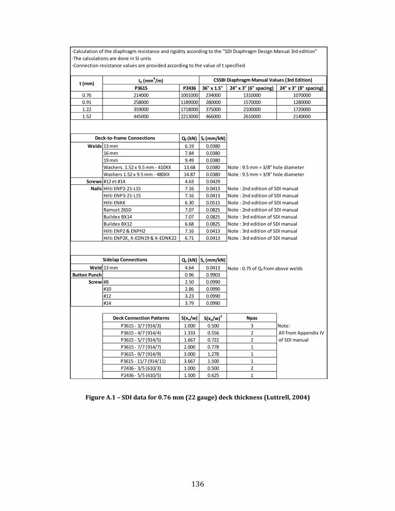
136

Figure A.1 – SDI data for 0.76 mm (22 gauge) deck thickness (Luttrell, 2004)

-Calculation of the diaphragm resistance and rigidity according to the "SDI Diaphragm Design Manual 3rd edition"-The calculations are done in SI units-Connection resistance values are provided according to the value of t specified

P3615 P2436 36" x 1.5" 24" x 3" (6" spacing) 24" x 3" (8" spacing)0.76 214000 1001000 234000 1310000 10700000.91 258000 1189000 280000 1570000 12800001.22 359000 1718000 375000 2100000 17200001.52 445000 2213000 466000 2610000 2140000

Qf (kN) Sf (mm/kN)

Welds 13 mm 6.19 0.038016 mm 7.84 0.038019 mm 9.49 0.0380Washers. 1.52 x 9.5 mm - 410XX 13.68 0.0380 Note : 9.5 mm = 3/8" hole diameterWashers 1.52 x 9.5 mm - 480XX 14.87 0.0380 Note : 9.5 mm = 3/8" hole diameter

Screws #12 et #14 4.63 0.0429Nails Hilti ENP2-21-L15 7.16 0.0413 Note : 2nd edition of SDI manual

Hilti ENP3-21-L15 7.16 0.0413 Note : 2nd edition of SDI manualHilti ENKK 6.30 0.0515 Note : 2nd edition of SDI manualRamset 26SD 7.07 0.0825 Note : 2nd edition of SDI manualBuildex BX14 7.07 0.0825 Note : 3rd edition of SDI manualBuildex BX12 6.68 0.0825 Note : 3rd edition of SDI manualHilti ENP2 & ENPH2 7.16 0.0413 Note : 3rd edition of SDI manualHilti ENP2K, X-EDN19 & X-EDNK22 6.71 0.0413 Note : 3rd edition of SDI manual

Qs (kN) Ss (mm/kN)

Weld 13 mm 4.64 0.0413 Note : 0.75 of Qf from above weldsButton Punch 0.96 0.9903

Screw #8 2.50 0.0990#10 2.86 0.0990#12 3.23 0.0990#14 3.79 0.0990

Deck Connection Patterns S(xe/w) S(xe/w)2 Npas

P3615 - 3/7 (914/3) 1.000 0.500 3 Note:P3615 - 4/7 (914/4) 1.333 0.556 2 All from Appendix IVP3615 - 5/7 (914/5) 1.667 0.722 2 of SDI manualP3615 - 7/7 (914/7) 2.000 0.778 1P3615 - 9/7 (914/9) 3.000 1.278 1

P3615 - 11/7 (914/11) 3.667 1.500 1P2436 - 3/5 (610/3) 1.000 0.500 2P2436 - 5/5 (610/5) 1.500 0.625 1

IX (mm4/m) CSSBI Diaphragm Manual Values (3rd Edition)

Deck-to-frame Connections

Sidelap Connections

t (mm)

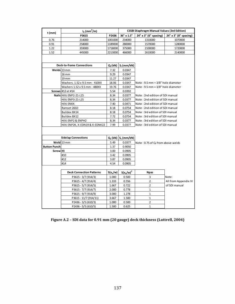
137

Figure A.2 – SDI data for 0.91 mm (20 gauge) deck thickness (Luttrell, 2004)

P3615 P2436 36" x 1.5" 24" x 3" (6" spacing) 24" x 3" (8" spacing)0.76 214000 1001000 234000 1310000 10700000.91 258000 1189000 280000 1570000 12800001.22 359000 1718000 375000 2100000 17200001.52 445000 2213000 466000 2610000 2140000

Qf (kN) Sf (mm/kN)

Welds 13 mm 7.32 0.034716 mm 9.29 0.034719 mm 11.27 0.0347Washers. 1.52 x 9.5 mm - 410XX 18.06 0.0347 Note : 9.5 mm = 3/8" hole diameterWashers 1.52 x 9.5 mm - 480XX 19.76 0.0347 Note : 9.5 mm = 3/8" hole diameter

Screws #12 et #14 5.54 0.0392Nails Hilti ENP2-21-L15 8.34 0.0377 Note : 2nd edition of SDI manual

Hilti ENP3-21-L15 8.34 0.0377 Note : 2nd edition of SDI manualHilti ENKK 7.40 0.0471 Note : 2nd edition of SDI manualRamset 26SD 8.18 0.0754 Note : 2nd edition of SDI manualBuildex BX14 8.18 0.0754 Note : 3rd edition of SDI manualBuildex BX12 7.72 0.0754 Note : 3rd edition of SDI manualHilti ENP2 & ENPH2 8.34 0.0377 Note : 3rd edition of SDI manualHilti ENP2K, X-EDN19 & X-EDNK22 7.99 0.0377 Note : 3rd edition of SDI manual

Qs (kN) Ss (mm/kN)

Weld 13 mm 5.49 0.0377 Note : 0.75 of Qf from above weldsButton Punch 1.37 0.9050

Screw #8 3.00 0.0905#10 3.42 0.0905#12 3.87 0.0905#14 4.54 0.0905

Deck Connection Patterns S(xe/w) S(xe/w)2 Npas

P3615 - 3/7 (914/3) 1.000 0.500 3 Note:P3615 - 4/7 (914/4) 1.333 0.556 2 All from Appendix IVP3615 - 5/7 (914/5) 1.667 0.722 2 of SDI manualP3615 - 7/7 (914/7) 2.000 0.778 1P3615 - 9/7 (914/9) 3.000 1.278 1

P3615 - 11/7 (914/11) 3.667 1.500 1P2436 - 3/5 (610/3) 1.000 0.500 2P2436 - 5/5 (610/5) 1.500 0.625 1

IX (mm4/m) CSSBI Diaphragm Manual Values (3rd Edition)

Deck-to-frame Connections

Sidelap Connections

t (mm)

138

Figure A.3 – SDI data for 1.21 mm (18 gauge) deck thickness (Luttrell, 2004)

P3615 P2436 36" x 1.5" 24" x 3" (6" spacing) 24" x 3" (8" spacing)0.76 214000 1001000 234000 1310000 10700000.91 258000 1189000 280000 1570000 12800001.22 359000 1718000 375000 2100000 17200001.52 445000 2213000 466000 2610000 2140000

Qf (kN) Sf (mm/kN)

Welds 13 mm 9.49 0.030116 mm 12.11 0.030119 mm 14.73 0.0301Washers. 1.52 x 9.5 mm - 410XX 28.48 0.0301 Note : 9.5 mm = 3/8" hole diameterWashers 1.52 x 9.5 mm - 480XX 31.48 0.0301 Note : 9.5 mm = 3/8" hole diameter

Screws #12 et #14 7.37 0.0340Nails Hilti ENP2-21-L15 10.48 0.0327 Note : 2nd edition of SDI manual

Hilti ENP3-21-L15 10.48 0.0327 Note : 2nd edition of SDI manualHilti ENKK 9.44 0.0408 Note : 2nd edition of SDI manualRamset 26SD 10.09 0.0654 Note : 2nd edition of SDI manualBuildex BX14 10.09 0.0654 Note : 3rd edition of SDI manualBuildex BX12 9.52 0.0654 Note : 3rd edition of SDI manualHilti ENP2 & ENPH2 10.48 0.0327 Note : 3rd edition of SDI manualHilti ENP2K, X-EDN19 & X-EDNK22 10.49 0.0327 Note : 3rd edition of SDI manual

Qs (kN) Ss (mm/kN)

Weld 13 mm 7.12 0.0327 Note : 0.75 of Qf from above weldsButton Punch 2.42 0.7849

Screw #8 3.98 0.0785#10 4.55 0.0785#12 5.14 0.0785#14 6.04 0.0785

Deck Connection Patterns S(xe/w) S(xe/w)2 Npas

P3615 - 3/7 (914/3) 1.000 0.500 3 Note:P3615 - 4/7 (914/4) 1.333 0.556 2 All from Appendix IVP3615 - 5/7 (914/5) 1.667 0.722 2 of SDI manualP3615 - 7/7 (914/7) 2.000 0.778 1P3615 - 9/7 (914/9) 3.000 1.278 1

P3615 - 11/7 (914/11) 3.667 1.500 1P2436 - 3/5 (610/3) 1.000 0.500 2P2436 - 5/5 (610/5) 1.500 0.625 1

IX (mm4/m) CSSBI Diaphragm Manual Values (3rd Edition)

Deck-to-frame Connections

Sidelap Connections

t (mm)

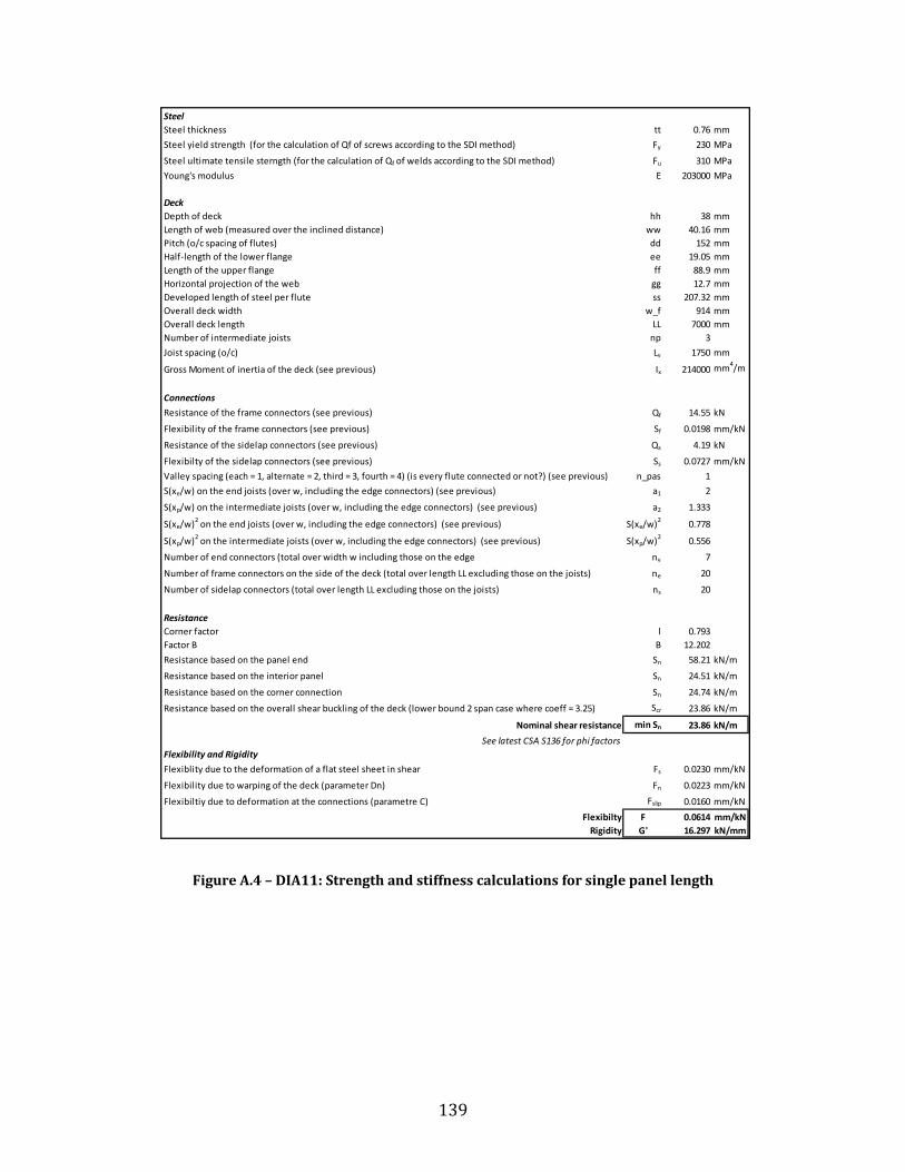
139

Figure A.4 – DIA11: Strength and stiffness calculations for single panel length

SteelSteel thickness tt 0.76 mm

Steel yield strength (for the calculation of Qf of screws according to the SDI method) Fy 230 MPa

Steel ultimate tensile sterngth (for the calculation of Qf of welds according to the SDI method) Fu 310 MPa

Young's modulus E 203000 MPa

DeckDepth of deck hh 38 mmLength of web (measured over the inclined distance) ww 40.16 mmPitch (o/c spacing of flutes) dd 152 mmHalf-length of the lower flange ee 19.05 mmLength of the upper flange ff 88.9 mmHorizontal projection of the web gg 12.7 mmDeveloped length of steel per flute ss 207.32 mmOverall deck width w_f 914 mmOverall deck length LL 7000 mmNumber of intermediate joists np 3

Joist spacing (o/c) Lv 1750 mm

Gross Moment of inertia of the deck (see previous) Ix 214000 mm4/m

Connections

Resistance of the frame connectors (see previous) Qf 14.55 kN

Flexibility of the frame connectors (see previous) Sf 0.0198 mm/kN

Resistance of the sidelap connectors (see previous) Qs 4.19 kN

Flexibilty of the sidelap connectors (see previous) Ss 0.0727 mm/kN

Valley spacing (each = 1, alternate = 2, third = 3, fourth = 4) (is every flute connected or not?) (see previous) n_pas 1

S(xe/w) on the end joists (over w, including the edge connectors) (see previous) a1 2

S(xp/w) on the intermediate joists (over w, including the edge connectors) (see previous) a2 1.333

S(xe/w)2 on the end joists (over w, including the edge connectors) (see previous) S(xe/w)2 0.778

S(xp/w)2 on the intermediate joists (over w, including the edge connectors) (see previous) S(xp/w)2 0.556

Number of end connectors (total over width w including those on the edge nv 7

Number of frame connectors on the side of the deck (total over length LL excluding those on the joists) ne 20

Number of sidelap connectors (total over length LL excluding those on the joists) ns 20

ResistanceCorner factor l 0.793Factor B B 12.202

Resistance based on the panel end Sn 58.21 kN/m

Resistance based on the interior panel Sn 24.51 kN/m

Resistance based on the corner connection Sn 24.74 kN/m

Resistance based on the overall shear buckling of the deck (lower bound 2 span case where coeff = 3.25) Scr 23.86 kN/m

Nominal shear resistance min Sn 23.86 kN/m

See latest CSA S136 for phi factorsFlexibility and Rigidity

Flexiblity due to the deformation of a flat steel sheet in shear Fs 0.0230 mm/kN

Flexibility due to warping of the deck (parameter Dn) Fn 0.0223 mm/kN

Flexibiltiy due to deformation at the connections (parametre C) Fslip 0.0160 mm/kN

Flexibilty F 0.0614 mm/kNRigidity G' 16.297 kN/mm

140

Figure A.5 – DIA11: Strength and stiffness calculations for three panel length

SteelSteel thickness tt 0.76 mm

Steel yield strength (for the calculation of Qf of screws according to the SDI method) Fy 230 MPa

Steel ultimate tensile sterngth (for the calculation of Qf of welds according to the SDI method) Fu 310 MPa

Young's modulus E 203000 MPa

DeckDepth of deck hh 38 mmLength of web (measured over the inclined distance) ww 40.16 mmPitch (o/c spacing of flutes) dd 152 mmHalf-length of the lower flange ee 19.05 mmLength of the upper flange ff 88.9 mmHorizontal projection of the web gg 12.7 mmDeveloped length of steel per flute ss 207.32 mmOverall deck width w_f 914 mmOverall deck length LL 21000 mmNumber of intermediate joists np 11

Joist spacing (o/c) Lv 1750 mm

Gross Moment of inertia of the deck (see previous) Ix 214000 mm4/m

Connections

Resistance of the frame connectors (see previous) Qf 14.55 kN

Flexibility of the frame connectors (see previous) Sf 0.0198 mm/kN

Resistance of the sidelap connectors (see previous) Qs 4.19 kN

Flexibilty of the sidelap connectors (see previous) Ss 0.0727 mm/kN

Valley spacing (each = 1, alternate = 2, third = 3, fourth = 4) (is every flute connected or not?) (see previous) n_pas 1

S(xe/w) on the end joists (over w, including the edge connectors) (see previous) a1 2

S(xp/w) on the intermediate joists (over w, including the edge connectors) (see previous) a2 1.333

S(xe/w)2 on the end joists (over w, including the edge connectors) (see previous) S(xe/w)2 0.778

S(xp/w)2 on the intermediate joists (over w, including the edge connectors) (see previous) S(xp/w)2 0.556

Number of end connectors (total over width w including those on the edge nv 7

Number of frame connectors on the side of the deck (total over length LL excluding those on the joists) ne 60

Number of sidelap connectors (total over length LL excluding those on the joists) ns 60

ResistanceCorner factor l 0.793Factor B B 32.605

Resistance based on the panel end Sn 54.52 kN/m

Resistance based on the interior panel Sn 22.31 kN/m

Resistance based on the corner connection Sn 22.15 kN/m

Resistance based on the overall shear buckling of the deck (lower bound 2 span case where coeff = 3.25) Scr 23.86 kN/m

Nominal shear resistance min Sn 22.15 kN/m

See latest CSA S136 for phi factorsFlexibility and Rigidity

Flexiblity due to the deformation of a flat steel sheet in shear Fs 0.0230 mm/kN

Flexibility due to warping of the deck (parameter Dn) Fn 0.0031 mm/kN

Flexibiltiy due to deformation at the connections (parametre C) Fslip 0.0177 mm/kN

Flexibilty F 0.0438 mm/kNRigidity G' 22.841 kN/mm

141

Figure A.6 – DIA12, DIA12R and DIA13R: Strength and stiffness calculations for single panel length

SteelSteel thickness tt 1.21 mm

Steel yield strength (for the calculation of Qf of screws according to the SDI method) Fy 230 MPa

Steel ultimate tensile sterngth (for the calculation of Qf of welds according to the SDI method) Fu 310 MPa

Young's modulus E 203000 MPa

DeckDepth of deck hh 38 mmLength of web (measured over the inclined distance) ww 40.16 mmPitch (o/c spacing of flutes) dd 152 mmHalf-length of the lower flange ee 19.05 mmLength of the upper flange ff 88.9 mmHorizontal projection of the web gg 12.7 mmDeveloped length of steel per flute ss 207.32 mmOverall deck width w_f 914 mmOverall deck length LL 7000 mmNumber of intermediate joists np 3

Joist spacing (o/c) Lv 1750 mm

Gross Moment of inertia of the deck (see previous) Ix 359000 mm4/m

Connections

Resistance of the frame connectors (see previous) Qf 10.49 kN

Flexibility of the frame connectors (see previous) Sf 0.0327 mm/kN

Resistance of the sidelap connectors (see previous) Qs 5.14 kN

Flexibilty of the sidelap connectors (see previous) Ss 0.0785 mm/kN

Valley spacing (each = 1, alternate = 2, third = 3, fourth = 4) (is every flute connected or not?) (see previous) n_pas 1

S(xe/w) on the end joists (over w, including the edge connectors) (see previous) a1 2

S(xp/w) on the intermediate joists (over w, including the edge connectors) (see previous) a2 2

S(xe/w)2 on the end joists (over w, including the edge connectors) (see previous) S(xe/w)2 0.778

S(xp/w)2 on the intermediate joists (over w, including the edge connectors) (see previous) S(xp/w)2 0.778

Number of end connectors (total over width w including those on the edge nv 7

Number of frame connectors on the side of the deck (total over length LL excluding those on the joists) ne 44

Number of sidelap connectors (total over length LL excluding those on the joists) ns 44

ResistanceCorner factor l 0.836Factor B B 29.340

Resistance based on the panel end Sn 80.92 kN/m

Resistance based on the interior panel Sn 43.48 kN/m

Resistance based on the corner connection Sn 38.57 kN/m

Resistance based on the overall shear buckling of the deck (lower bound 2 span case where coeff = 3.25) Scr 49.84 kN/m

Nominal shear resistance min Sn 38.57 kN/m

See latest CSA S136 for phi factorsFlexibility and Rigidity

Flexiblity due to the deformation of a flat steel sheet in shear Fs 0.0144 mm/kN

Flexibility due to warping of the deck (parameter Dn) Fn 0.0070 mm/kN

Flexibiltiy due to deformation at the connections (parametre C) Fslip 0.0107 mm/kN

Flexibilty F 0.0322 mm/kNRigidity G' 31.101 kN/mm

142

Figure A.7 – DIA12, DIA12R and DIA13R: Strength and stiffness calculations for three panel length

SteelSteel thickness tt 1.21 mm

Steel yield strength (for the calculation of Qf of screws according to the SDI method) Fy 230 MPa

Steel ultimate tensile sterngth (for the calculation of Qf of welds according to the SDI method) Fu 310 MPa

Young's modulus E 203000 MPa

DeckDepth of deck hh 38 mmLength of web (measured over the inclined distance) ww 40.16 mmPitch (o/c spacing of flutes) dd 152 mmHalf-length of the lower flange ee 19.05 mmLength of the upper flange ff 88.9 mmHorizontal projection of the web gg 12.7 mmDeveloped length of steel per flute ss 207.32 mmOverall deck width w_f 914 mmOverall deck length LL 21000 mmNumber of intermediate joists np 11

Joist spacing (o/c) Lv 1750 mm

Gross Moment of inertia of the deck (see previous) Ix 359000 mm4/m

Connections

Resistance of the frame connectors (see previous) Qf 10.49 kN

Flexibility of the frame connectors (see previous) Sf 0.0327 mm/kN

Resistance of the sidelap connectors (see previous) Qs 5.14 kN

Flexibilty of the sidelap connectors (see previous) Ss 0.0785 mm/kN

Valley spacing (each = 1, alternate = 2, third = 3, fourth = 4) (is every flute connected or not?) (see previous) n_pas 1

S(xe/w) on the end joists (over w, including the edge connectors) (see previous) a1 2

S(xp/w) on the intermediate joists (over w, including the edge connectors) (see previous) a2 2

S(xe/w)2 on the end joists (over w, including the edge connectors) (see previous) S(xe/w)2 0.778

S(xp/w)2 on the intermediate joists (over w, including the edge connectors) (see previous) S(xp/w)2 0.778

Number of end connectors (total over width w including those on the edge nv 7

Number of frame connectors on the side of the deck (total over length LL excluding those on the joists) ne 132

Number of sidelap connectors (total over length LL excluding those on the joists) ns 132

ResistanceCorner factor l 0.836Factor B B 84.907

Resistance based on the panel end Sn 78.92 kN/m

Resistance based on the interior panel Sn 42.25 kN/m

Resistance based on the corner connection Sn 37.51 kN/m

Resistance based on the overall shear buckling of the deck (lower bound 2 span case where coeff = 3.25) Scr 49.84 kN/m

Nominal shear resistance min Sn 37.51 kN/m

See latest CSA S136 for phi factorsFlexibility and Rigidity

Flexiblity due to the deformation of a flat steel sheet in shear Fs 0.0144 mm/kN

Flexibility due to warping of the deck (parameter Dn) Fn 0.0010 mm/kN

Flexibiltiy due to deformation at the connections (parametre C) Fslip 0.0111 mm/kN

Flexibilty F 0.0265 mm/kNRigidity G' 37.806 kN/mm

143

Figure A.8 – DIA13: Strength and stiffness calculations for single panel length

SteelSteel thickness tt 1.21 mm

Steel yield strength (for the calculation of Qf of screws according to the SDI method) Fy 230 MPa

Steel ultimate tensile sterngth (for the calculation of Qf of welds according to the SDI method) Fu 310 MPa

Young's modulus E 203000 MPa

DeckDepth of deck hh 38 mmLength of web (measured over the inclined distance) ww 40.16 mmPitch (o/c spacing of flutes) dd 152 mmHalf-length of the lower flange ee 19.05 mmLength of the upper flange ff 88.9 mmHorizontal projection of the web gg 12.7 mmDeveloped length of steel per flute ss 207.32 mmOverall deck width w_f 914 mmOverall deck length LL 7000 mmNumber of intermediate joists np 3

Joist spacing (o/c) Lv 1750 mm

Gross Moment of inertia of the deck (see previous) Ix 359000 mm4/m

Connections

Resistance of the frame connectors (see previous) Qf 14.73 kN

Flexibility of the frame connectors (see previous) Sf 0.0301 mm/kN

Resistance of the sidelap connectors (see previous) Qs 5.14 kN

Flexibilty of the sidelap connectors (see previous) Ss 0.0785 mm/kN

Valley spacing (each = 1, alternate = 2, third = 3, fourth = 4) (is every flute connected or not?) (see previous) n_pas 1

S(xe/w) on the end joists (over w, including the edge connectors) (see previous) a1 2

S(xp/w) on the intermediate joists (over w, including the edge connectors) (see previous) a2 2

S(xe/w)2 on the end joists (over w, including the edge connectors) (see previous) S(xe/w)2 0.778

S(xp/w)2 on the intermediate joists (over w, including the edge connectors) (see previous) S(xp/w)2 0.778

Number of end connectors (total over width w including those on the edge nv 7

Number of frame connectors on the side of the deck (total over length LL excluding those on the joists) ne 44

Number of sidelap connectors (total over length LL excluding those on the joists) ns 44

ResistanceCorner factor l 0.836Factor B B 23.134

Resistance based on the panel end Sn 113.63 kN/m

Resistance based on the interior panel Sn 47.99 kN/m

Resistance based on the corner connection Sn 44.70 kN/m

Resistance based on the overall shear buckling of the deck (lower bound 2 span case where coeff = 3.25) Scr 49.84 kN/m

Nominal shear resistance min Sn 44.70 kN/m

See latest CSA S136 for phi factorsFlexibility and Rigidity

Flexiblity due to the deformation of a flat steel sheet in shear Fs 0.0144 mm/kN

Flexibility due to warping of the deck (parameter Dn) Fn 0.0070 mm/kN

Flexibiltiy due to deformation at the connections (parametre C) Fslip 0.0105 mm/kN

Flexibilty F 0.0320 mm/kNRigidity G' 31.291 kN/mm

144

Figure A.9 – DIA13: Strength and stiffness calculations for three panel length

SteelSteel thickness tt 1.21 mm

Steel yield strength (for the calculation of Qf of screws according to the SDI method) Fy 230 MPa

Steel ultimate tensile sterngth (for the calculation of Qf of welds according to the SDI method) Fu 310 MPa

Young's modulus E 203000 MPa

DeckDepth of deck hh 38 mmLength of web (measured over the inclined distance) ww 40.16 mmPitch (o/c spacing of flutes) dd 152 mmHalf-length of the lower flange ee 19.05 mmLength of the upper flange ff 88.9 mmHorizontal projection of the web gg 12.7 mmDeveloped length of steel per flute ss 207.32 mmOverall deck width w_f 914 mmOverall deck length LL 21000 mmNumber of intermediate joists np 11

Joist spacing (o/c) Lv 1750 mm

Gross Moment of inertia of the deck (see previous) Ix 359000 mm4/m

Connections

Resistance of the frame connectors (see previous) Qf 14.73 kN

Flexibility of the frame connectors (see previous) Sf 0.0301 mm/kN

Resistance of the sidelap connectors (see previous) Qs 5.14 kN

Flexibilty of the sidelap connectors (see previous) Ss 0.0785 mm/kN

Valley spacing (each = 1, alternate = 2, third = 3, fourth = 4) (is every flute connected or not?) (see previous) n_pas 1

S(xe/w) on the end joists (over w, including the edge connectors) (see previous) a1 2

S(xp/w) on the intermediate joists (over w, including the edge connectors) (see previous) a2 2

S(xe/w)2 on the end joists (over w, including the edge connectors) (see previous) S(xe/w)2 0.778

S(xp/w)2 on the intermediate joists (over w, including the edge connectors) (see previous) S(xp/w)2 0.778

Number of end connectors (total over width w including those on the edge nv 7

Number of frame connectors on the side of the deck (total over length LL excluding those on the joists) ne 132

Number of sidelap connectors (total over length LL excluding those on the joists) ns 132

ResistanceCorner factor l 0.836Factor B B 66.289

Resistance based on the panel end Sn 110.83 kN/m

Resistance based on the interior panel Sn 46.27 kN/m

Resistance based on the corner connection Sn 42.99 kN/m

Resistance based on the overall shear buckling of the deck (lower bound 2 span case where coeff = 3.25) Scr 49.84 kN/m

Nominal shear resistance min Sn 42.99 kN/m

See latest CSA S136 for phi factorsFlexibility and Rigidity

Flexiblity due to the deformation of a flat steel sheet in shear Fs 0.0144 mm/kN

Flexibility due to warping of the deck (parameter Dn) Fn 0.0010 mm/kN

Flexibiltiy due to deformation at the connections (parametre C) Fslip 0.0109 mm/kN

Flexibilty F 0.0263 mm/kNRigidity G' 38.064 kN/mm

145

Figure A.10 – DIA14: Strength and stiffness calculations for single panel length

SteelSteel thickness tt 1.21 mm

Steel yield strength (for the calculation of Qf of screws according to the SDI method) Fy 230 MPa

Steel ultimate tensile sterngth (for the calculation of Qf of welds according to the SDI method) Fu 310 MPa

Young's modulus E 203000 MPa

DeckDepth of deck hh 38 mmLength of web (measured over the inclined distance) ww 40.16 mmPitch (o/c spacing of flutes) dd 152 mmHalf-length of the lower flange ee 19.05 mmLength of the upper flange ff 88.9 mmHorizontal projection of the web gg 12.7 mmDeveloped length of steel per flute ss 207.32 mmOverall deck width w_f 914 mmOverall deck length LL 7000 mmNumber of intermediate joists np 3

Joist spacing (o/c) Lv 1750 mm

Gross Moment of inertia of the deck (see previous) Ix 359000 mm4/m

Connections

Resistance of the frame connectors (see previous) Qf 10.49 kN

Flexibility of the frame connectors (see previous) Sf 0.0327 mm/kN

Resistance of the sidelap connectors (see previous) Qs 5.14 kN

Flexibilty of the sidelap connectors (see previous) Ss 0.0785 mm/kN

Valley spacing (each = 1, alternate = 2, third = 3, fourth = 4) (is every flute connected or not?) (see previous) n_pas 1

S(xe/w) on the end joists (over w, including the edge connectors) (see previous) a1 3

S(xp/w) on the intermediate joists (over w, including the edge connectors) (see previous) a2 3

S(xe/w)2 on the end joists (over w, including the edge connectors) (see previous) S(xe/w)2 1.278

S(xp/w)2 on the intermediate joists (over w, including the edge connectors) (see previous) S(xp/w)2 1.278

Number of end connectors (total over width w including those on the edge nv 9

Number of frame connectors on the side of the deck (total over length LL excluding those on the joists) ne 64

Number of sidelap connectors (total over length LL excluding those on the joists) ns 64

ResistanceCorner factor l 0.836Factor B B 44.139

Resistance based on the panel end Sn 118.39 kN/m

Resistance based on the interior panel Sn 65.65 kN/m

Resistance based on the corner connection Sn 55.70 kN/m

Resistance based on the overall shear buckling of the deck (lower bound 2 span case where coeff = 3.25) Scr 49.84 kN/m

Nominal shear resistance min Sn 49.84 kN/m

See latest CSA S136 for phi factorsFlexibility and Rigidity

Flexiblity due to the deformation of a flat steel sheet in shear Fs 0.0144 mm/kN

Flexibility due to warping of the deck (parameter Dn) Fn 0.0070 mm/kN

Flexibiltiy due to deformation at the connections (parametre C) Fslip 0.0073 mm/kN

Flexibilty F 0.0287 mm/kNRigidity G' 34.783 kN/mm

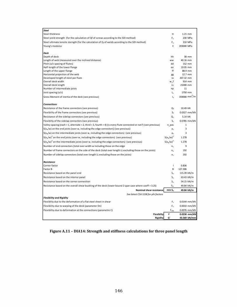
146

Figure A.11 – DIA14: Strength and stiffness calculations for three panel length

SteelSteel thickness tt 1.21 mm

Steel yield strength (for the calculation of Qf of screws according to the SDI method) Fy 230 MPa

Steel ultimate tensile sterngth (for the calculation of Qf of welds according to the SDI method) Fu 310 MPa

Young's modulus E 203000 MPa

DeckDepth of deck hh 38 mmLength of web (measured over the inclined distance) ww 40.16 mmPitch (o/c spacing of flutes) dd 152 mmHalf-length of the lower flange ee 19.05 mmLength of the upper flange ff 88.9 mmHorizontal projection of the web gg 12.7 mmDeveloped length of steel per flute ss 207.32 mmOverall deck width w_f 914 mmOverall deck length LL 21000 mmNumber of intermediate joists np 11

Joist spacing (o/c) Lv 1750 mm

Gross Moment of inertia of the deck (see previous) Ix 359000 mm4/m

Connections

Resistance of the frame connectors (see previous) Qf 10.49 kN

Flexibility of the frame connectors (see previous) Sf 0.0327 mm/kN

Resistance of the sidelap connectors (see previous) Qs 5.14 kN

Flexibilty of the sidelap connectors (see previous) Ss 0.0785 mm/kN

Valley spacing (each = 1, alternate = 2, third = 3, fourth = 4) (is every flute connected or not?) (see previous) n_pas 1

S(xe/w) on the end joists (over w, including the edge connectors) (see previous) a1 3

S(xp/w) on the intermediate joists (over w, including the edge connectors) (see previous) a2 3

S(xe/w)2 on the end joists (over w, including the edge connectors) (see previous) S(xe/w)2 1.278

S(xp/w)2 on the intermediate joists (over w, including the edge connectors) (see previous) S(xp/w)2 1.278

Number of end connectors (total over width w including those on the edge nv 9

Number of frame connectors on the side of the deck (total over length LL excluding those on the joists) ne 192

Number of sidelap connectors (total over length LL excluding those on the joists) ns 192

ResistanceCorner factor l 0.836Factor B B 127.306

Resistance based on the panel end Sn 115.39 kN/m

Resistance based on the interior panel Sn 63.43 kN/m

Resistance based on the corner connection Sn 54.15 kN/m

Resistance based on the overall shear buckling of the deck (lower bound 2 span case where coeff = 3.25) Scr 49.84 kN/m

Nominal shear resistance min Sn 49.84 kN/m

See latest CSA S136 for phi factorsFlexibility and Rigidity

Flexiblity due to the deformation of a flat steel sheet in shear Fs 0.0144 mm/kN

Flexibility due to warping of the deck (parameter Dn) Fn 0.0010 mm/kN

Flexibiltiy due to deformation at the connections (parametre C) Fslip 0.0076 mm/kN

Flexibilty F 0.0230 mm/kNRigidity G' 43.569 kN/mm

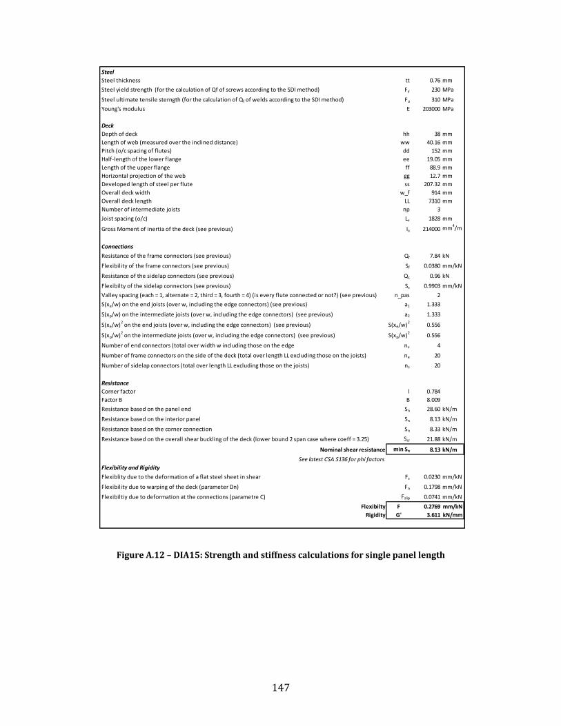
147

Figure A.12 – DIA15: Strength and stiffness calculations for single panel length

SteelSteel thickness tt 0.76 mm

Steel yield strength (for the calculation of Qf of screws according to the SDI method) Fy 230 MPa

Steel ultimate tensile sterngth (for the calculation of Qf of welds according to the SDI method) Fu 310 MPa

Young's modulus E 203000 MPa

DeckDepth of deck hh 38 mmLength of web (measured over the inclined distance) ww 40.16 mmPitch (o/c spacing of flutes) dd 152 mmHalf-length of the lower flange ee 19.05 mmLength of the upper flange ff 88.9 mmHorizontal projection of the web gg 12.7 mmDeveloped length of steel per flute ss 207.32 mmOverall deck width w_f 914 mmOverall deck length LL 7310 mmNumber of intermediate joists np 3

Joist spacing (o/c) Lv 1828 mm

Gross Moment of inertia of the deck (see previous) Ix 214000 mm4/m

Connections

Resistance of the frame connectors (see previous) Qf 7.84 kN

Flexibility of the frame connectors (see previous) Sf 0.0380 mm/kN

Resistance of the sidelap connectors (see previous) Qs 0.96 kN

Flexibilty of the sidelap connectors (see previous) Ss 0.9903 mm/kN

Valley spacing (each = 1, alternate = 2, third = 3, fourth = 4) (is every flute connected or not?) (see previous) n_pas 2

S(xe/w) on the end joists (over w, including the edge connectors) (see previous) a1 1.333

S(xp/w) on the intermediate joists (over w, including the edge connectors) (see previous) a2 1.333

S(xe/w)2 on the end joists (over w, including the edge connectors) (see previous) S(xe/w)2 0.556

S(xp/w)2 on the intermediate joists (over w, including the edge connectors) (see previous) S(xp/w)2 0.556

Number of end connectors (total over width w including those on the edge nv 4

Number of frame connectors on the side of the deck (total over length LL excluding those on the joists) ne 20

Number of sidelap connectors (total over length LL excluding those on the joists) ns 20

ResistanceCorner factor l 0.784Factor B B 8.009

Resistance based on the panel end Sn 28.60 kN/m

Resistance based on the interior panel Sn 8.13 kN/m

Resistance based on the corner connection Sn 8.33 kN/m

Resistance based on the overall shear buckling of the deck (lower bound 2 span case where coeff = 3.25) Scr 21.88 kN/m

Nominal shear resistance min Sn 8.13 kN/m

See latest CSA S136 for phi factorsFlexibility and Rigidity

Flexiblity due to the deformation of a flat steel sheet in shear Fs 0.0230 mm/kN

Flexibility due to warping of the deck (parameter Dn) Fn 0.1798 mm/kN

Flexibiltiy due to deformation at the connections (parametre C) Fslip 0.0741 mm/kN

Flexibilty F 0.2769 mm/kNRigidity G' 3.611 kN/mm

148

Figure A.13 – DIA15R: Strength and stiffness calculations for single panel length

SteelSteel thickness tt 0.76 mm

Steel yield strength (for the calculation of Qf of screws according to the SDI method) Fy 230 MPa

Steel ultimate tensile sterngth (for the calculation of Qf of welds according to the SDI method) Fu 310 MPa

Young's modulus E 203000 MPa

DeckDepth of deck hh 38 mmLength of web (measured over the inclined distance) ww 40.16 mmPitch (o/c spacing of flutes) dd 152 mmHalf-length of the lower flange ee 19.05 mmLength of the upper flange ff 88.9 mmHorizontal projection of the web gg 12.7 mmDeveloped length of steel per flute ss 207.32 mmOverall deck width w_f 914 mmOverall deck length LL 7310 mmNumber of intermediate joists np 3

Joist spacing (o/c) Lv 1828 mm

Gross Moment of inertia of the deck (see previous) Ix 214000 mm4/m

Connections

Resistance of the frame connectors (see previous) Qf 6.71 kN

Flexibility of the frame connectors (see previous) Sf 0.0413 mm/kN

Resistance of the sidelap connectors (see previous) Qs 3.23 kN

Flexibilty of the sidelap connectors (see previous) Ss 0.0990 mm/kN

Valley spacing (each = 1, alternate = 2, third = 3, fourth = 4) (is every flute connected or not?) (see previous) n_pas 2

S(xe/w) on the end joists (over w, including the edge connectors) (see previous) a1 1.333

S(xp/w) on the intermediate joists (over w, including the edge connectors) (see previous) a2 1.333

S(xe/w)2 on the end joists (over w, including the edge connectors) (see previous) S(xe/w)2 0.556

S(xp/w)2 on the intermediate joists (over w, including the edge connectors) (see previous) S(xp/w)2 0.556

Number of end connectors (total over width w including those on the edge nv 4

Number of frame connectors on the side of the deck (total over length LL excluding those on the joists) ne 20

Number of sidelap connectors (total over length LL excluding those on the joists) ns 20

ResistanceCorner factor l 0.784Factor B B 15.187

Resistance based on the panel end Sn 24.48 kN/m

Resistance based on the interior panel Sn 13.54 kN/m

Resistance based on the corner connection Sn 12.59 kN/m

Resistance based on the overall shear buckling of the deck (lower bound 2 span case where coeff = 3.25) Scr 21.88 kN/m

Nominal shear resistance min Sn 12.59 kN/m

See latest CSA S136 for phi factorsFlexibility and Rigidity

Flexiblity due to the deformation of a flat steel sheet in shear Fs 0.0230 mm/kN

Flexibility due to warping of the deck (parameter Dn) Fn 0.1798 mm/kN

Flexibiltiy due to deformation at the connections (parametre C) Fslip 0.0283 mm/kN

Flexibilty F 0.2311 mm/kNRigidity G' 4.327 kN/mm

149

Figure A.14 – DIA16: Strength and stiffness calculations for single panel length

SteelSteel thickness tt 0.76 mm

Steel yield strength (for the calculation of Qf of screws according to the SDI method) Fy 230 MPa

Steel ultimate tensile sterngth (for the calculation of Qf of welds according to the SDI method) Fu 310 MPa

Young's modulus E 203000 MPa

DeckDepth of deck hh 38 mmLength of web (measured over the inclined distance) ww 40.16 mmPitch (o/c spacing of flutes) dd 152 mmHalf-length of the lower flange ee 19.05 mmLength of the upper flange ff 88.9 mmHorizontal projection of the web gg 12.7 mmDeveloped length of steel per flute ss 207.32 mmOverall deck width w_f 914 mmOverall deck length LL 7310 mmNumber of intermediate joists np 3

Joist spacing (o/c) Lv 1828 mm

Gross Moment of inertia of the deck (see previous) Ix 214000 mm4/m

Connections

Resistance of the frame connectors (see previous) Qf 6.71 kN

Flexibility of the frame connectors (see previous) Sf 0.0413 mm/kN

Resistance of the sidelap connectors (see previous) Qs 3.23 kN

Flexibilty of the sidelap connectors (see previous) Ss 0.0990 mm/kN

Valley spacing (each = 1, alternate = 2, third = 3, fourth = 4) (is every flute connected or not?) (see previous) n_pas 1

S(xe/w) on the end joists (over w, including the edge connectors) (see previous) a1 2

S(xp/w) on the intermediate joists (over w, including the edge connectors) (see previous) a2 2

S(xe/w)2 on the end joists (over w, including the edge connectors) (see previous) S(xe/w)2 0.778

S(xp/w)2 on the intermediate joists (over w, including the edge connectors) (see previous) S(xp/w)2 0.778

Number of end connectors (total over width w including those on the edge nv 7

Number of frame connectors on the side of the deck (total over length LL excluding those on the joists) ne 44

Number of sidelap connectors (total over length LL excluding those on the joists) ns 44

ResistanceCorner factor l 0.784Factor B B 28.960

Resistance based on the panel end Sn 49.57 kN/m

Resistance based on the interior panel Sn 26.19 kN/m

Resistance based on the corner connection Sn 23.61 kN/m

Resistance based on the overall shear buckling of the deck (lower bound 2 span case where coeff = 3.25) Scr 21.88 kN/m

Nominal shear resistance min Sn 21.88 kN/m

See latest CSA S136 for phi factorsFlexibility and Rigidity

Flexiblity due to the deformation of a flat steel sheet in shear Fs 0.0230 mm/kN

Flexibility due to warping of the deck (parameter Dn) Fn 0.0214 mm/kN

Flexibiltiy due to deformation at the connections (parametre C) Fslip 0.0141 mm/kN

Flexibilty F 0.0585 mm/kNRigidity G' 17.091 kN/mm

150

Figure A.15 – DIA16R: Strength and stiffness calculations for single panel length

SteelSteel thickness tt 0.76 mm

Steel yield strength (for the calculation of Qf of screws according to the SDI method) Fy 230 MPa

Steel ultimate tensile sterngth (for the calculation of Qf of welds according to the SDI method) Fu 310 MPa

Young's modulus E 203000 MPa

DeckDepth of deck hh 38 mmLength of web (measured over the inclined distance) ww 40.16 mmPitch (o/c spacing of flutes) dd 152 mmHalf-length of the lower flange ee 19.05 mmLength of the upper flange ff 88.9 mmHorizontal projection of the web gg 12.7 mmDeveloped length of steel per flute ss 207.32 mmOverall deck width w_f 914 mmOverall deck length LL 7310 mmNumber of intermediate joists np 3

Joist spacing (o/c) Lv 1828 mm

Gross Moment of inertia of the deck (see previous) Ix 214000 mm4/m

Connections

Resistance of the frame connectors (see previous) Qf 6.71 kN

Flexibility of the frame connectors (see previous) Sf 0.0413 mm/kN

Resistance of the sidelap connectors (see previous) Qs 3.23 kN

Flexibilty of the sidelap connectors (see previous) Ss 0.0990 mm/kN

Valley spacing (each = 1, alternate = 2, third = 3, fourth = 4) (is every flute connected or not?) (see previous) n_pas 1

S(xe/w) on the end joists (over w, including the edge connectors) (see previous) a1 3

S(xp/w) on the intermediate joists (over w, including the edge connectors) (see previous) a2 3

S(xe/w)2 on the end joists (over w, including the edge connectors) (see previous) S(xe/w)2 1.278

S(xp/w)2 on the intermediate joists (over w, including the edge connectors) (see previous) S(xp/w)2 1.278

Number of end connectors (total over width w including those on the edge nv 9

Number of frame connectors on the side of the deck (total over length LL excluding those on the joists) ne 44

Number of sidelap connectors (total over length LL excluding those on the joists) ns 44

ResistanceCorner factor l 0.784Factor B B 33.960

Resistance based on the panel end Sn 54.16 kN/m

Resistance based on the interior panel Sn 30.78 kN/m

Resistance based on the corner connection Sn 28.19 kN/m

Resistance based on the overall shear buckling of the deck (lower bound 2 span case where coeff = 3.25) Scr 21.88 kN/m

Nominal shear resistance min Sn 21.88 kN/m

See latest CSA S136 for phi factorsFlexibility and Rigidity

Flexiblity due to the deformation of a flat steel sheet in shear Fs 0.0230 mm/kN

Flexibility due to warping of the deck (parameter Dn) Fn 0.0214 mm/kN

Flexibiltiy due to deformation at the connections (parametre C) Fslip 0.0128 mm/kN

Flexibilty F 0.0571 mm/kNRigidity G' 17.500 kN/mm

151

Figure A.16 – DIA17: Strength and stiffness calculations for single panel length

SteelSteel thickness tt 0.91 mm

Steel yield strength (for the calculation of Qf of screws according to the SDI method) Fy 230 MPa

Steel ultimate tensile sterngth (for the calculation of Qf of welds according to the SDI method) Fu 310 MPa

Young's modulus E 203000 MPa

DeckDepth of deck hh 38 mmLength of web (measured over the inclined distance) ww 40.16 mmPitch (o/c spacing of flutes) dd 152 mmHalf-length of the lower flange ee 19.05 mmLength of the upper flange ff 88.9 mmHorizontal projection of the web gg 12.7 mmDeveloped length of steel per flute ss 207.32 mmOverall deck width w_f 914 mmOverall deck length LL 7310 mmNumber of intermediate joists np 3

Joist spacing (o/c) Lv 1828 mm

Gross Moment of inertia of the deck (see previous) Ix 258000 mm4/m

Connections

Resistance of the frame connectors (see previous) Qf 7.99 kN

Flexibility of the frame connectors (see previous) Sf 0.0377 mm/kN

Resistance of the sidelap connectors (see previous) Qs 3.87 kN

Flexibilty of the sidelap connectors (see previous) Ss 0.0905 mm/kN

Valley spacing (each = 1, alternate = 2, third = 3, fourth = 4) (is every flute connected or not?) (see previous) n_pas 1

S(xe/w) on the end joists (over w, including the edge connectors) (see previous) a1 2

S(xp/w) on the intermediate joists (over w, including the edge connectors) (see previous) a2 2

S(xe/w)2 on the end joists (over w, including the edge connectors) (see previous) S(xe/w)2 0.778

S(xp/w)2 on the intermediate joists (over w, including the edge connectors) (see previous) S(xp/w)2 0.778

Number of end connectors (total over width w including those on the edge nv 7

Number of frame connectors on the side of the deck (total over length LL excluding those on the joists) ne 44

Number of sidelap connectors (total over length LL excluding those on the joists) ns 44

ResistanceCorner factor l 0.803Factor B B 29.092

Resistance based on the panel end Sn 59.02 kN/m

Resistance based on the interior panel Sn 31.37 kN/m

Resistance based on the corner connection Sn 28.22 kN/m

Resistance based on the overall shear buckling of the deck (lower bound 2 span case where coeff = 3.25) Scr 28.81 kN/m

Nominal shear resistance min Sn 28.22 kN/m

See latest CSA S136 for phi factorsFlexibility and Rigidity

Flexiblity due to the deformation of a flat steel sheet in shear Fs 0.0192 mm/kN

Flexibility due to warping of the deck (parameter Dn) Fn 0.0136 mm/kN

Flexibiltiy due to deformation at the connections (parametre C) Fslip 0.0129 mm/kN

Flexibilty F 0.0457 mm/kNRigidity G' 21.858 kN/mm

152

Figure A.17 – DIA17R: Strength and stiffness calculations for single panel length

SteelSteel thickness tt 0.91 mm

Steel yield strength (for the calculation of Qf of screws according to the SDI method) Fy 230 MPa

Steel ultimate tensile sterngth (for the calculation of Qf of welds according to the SDI method) Fu 310 MPa

Young's modulus E 203000 MPa

DeckDepth of deck hh 38 mmLength of web (measured over the inclined distance) ww 40.16 mmPitch (o/c spacing of flutes) dd 152 mmHalf-length of the lower flange ee 19.05 mmLength of the upper flange ff 88.9 mmHorizontal projection of the web gg 12.7 mmDeveloped length of steel per flute ss 207.32 mmOverall deck width w_f 914 mmOverall deck length LL 7310 mmNumber of intermediate joists np 3

Joist spacing (o/c) Lv 1828 mm

Gross Moment of inertia of the deck (see previous) Ix 258000 mm4/m

Connections

Resistance of the frame connectors (see previous) Qf 7.99 kN

Flexibility of the frame connectors (see previous) Sf 0.0377 mm/kN

Resistance of the sidelap connectors (see previous) Qs 3.87 kN

Flexibilty of the sidelap connectors (see previous) Ss 0.0905 mm/kN

Valley spacing (each = 1, alternate = 2, third = 3, fourth = 4) (is every flute connected or not?) (see previous) n_pas 1

S(xe/w) on the end joists (over w, including the edge connectors) (see previous) a1 3

S(xp/w) on the intermediate joists (over w, including the edge connectors) (see previous) a2 3

S(xe/w)2 on the end joists (over w, including the edge connectors) (see previous) S(xe/w)2 1.278

S(xp/w)2 on the intermediate joists (over w, including the edge connectors) (see previous) S(xp/w)2 1.278

Number of end connectors (total over width w including those on the edge nv 9

Number of frame connectors on the side of the deck (total over length LL excluding those on the joists) ne 44

Number of sidelap connectors (total over length LL excluding those on the joists) ns 44

ResistanceCorner factor l 0.803Factor B B 34.092

Resistance based on the panel end Sn 64.49 kN/m

Resistance based on the interior panel Sn 36.83 kN/m

Resistance based on the corner connection Sn 33.68 kN/m

Resistance based on the overall shear buckling of the deck (lower bound 2 span case where coeff = 3.25) Scr 28.81 kN/m

Nominal shear resistance min Sn 28.81 kN/m

See latest CSA S136 for phi factorsFlexibility and Rigidity

Flexiblity due to the deformation of a flat steel sheet in shear Fs 0.0192 mm/kN

Flexibility due to warping of the deck (parameter Dn) Fn 0.0136 mm/kN

Flexibiltiy due to deformation at the connections (parametre C) Fslip 0.0117 mm/kN

Flexibilty F 0.0445 mm/kNRigidity G' 22.473 kN/mm

153

Figure A.18 – DIA18: Strength and stiffness calculations of the end panel for single panel length

SteelSteel thickness tt 0.91 mm

Steel yield strength (for the calculation of Qf of screws according to the SDI method) Fy 230 MPa

Steel ultimate tensile sterngth (for the calculation of Qf of welds according to the SDI method) Fu 310 MPa

Young's modulus E 203000 MPa

DeckDepth of deck hh 38 mmLength of web (measured over the inclined distance) ww 40.16 mmPitch (o/c spacing of flutes) dd 152 mmHalf-length of the lower flange ee 19.05 mmLength of the upper flange ff 88.9 mmHorizontal projection of the web gg 12.7 mmDeveloped length of steel per flute ss 207.32 mmOverall deck width w_f 914 mmOverall deck length LL 7310 mmNumber of intermediate joists np 3

Joist spacing (o/c) Lv 1828 mm

Gross Moment of inertia of the deck (see previous) Ix 258000 mm4/m

Connections

Resistance of the frame connectors (see previous) Qf 7.99 kN

Flexibility of the frame connectors (see previous) Sf 0.0377 mm/kN

Resistance of the sidelap connectors (see previous) Qs 3.87 kN

Flexibilty of the sidelap connectors (see previous) Ss 0.0905 mm/kN

Valley spacing (each = 1, alternate = 2, third = 3, fourth = 4) (is every flute connected or not?) (see previous) n_pas 1

S(xe/w) on the end joists (over w, including the edge connectors) (see previous) a1 2

S(xp/w) on the intermediate joists (over w, including the edge connectors) (see previous) a2 2

S(xe/w)2 on the end joists (over w, including the edge connectors) (see previous) S(xe/w)2 0.778

S(xp/w)2 on the intermediate joists (over w, including the edge connectors) (see previous) S(xp/w)2 0.778

Number of end connectors (total over width w including those on the edge nv 7

Number of frame connectors on the side of the deck (total over length LL excluding those on the joists) ne 64

Number of sidelap connectors (total over length LL excluding those on the joists) ns 64

ResistanceCorner factor l 0.803Factor B B 38.779

Resistance based on the panel end Sn 80.88 kN/m

Resistance based on the interior panel Sn 41.95 kN/m

Resistance based on the corner connection Sn 34.84 kN/m

Resistance based on the overall shear buckling of the deck (lower bound 2 span case where coeff = 3.25) Scr 28.81 kN/m

Nominal shear resistance min Sn 28.81 kN/m

See latest CSA S136 for phi factorsFlexibility and Rigidity

Flexiblity due to the deformation of a flat steel sheet in shear Fs 0.0192 mm/kN

Flexibility due to warping of the deck (parameter Dn) Fn 0.0136 mm/kN

Flexibiltiy due to deformation at the connections (parametre C) Fslip 0.0095 mm/kN

Flexibilty F 0.0423 mm/kNRigidity G' 23.613 kN/mm

154

Figure A.19 – DIA18R: Strength and stiffness calculations for single panel length

SteelSteel thickness tt 0.91 mm

Steel yield strength (for the calculation of Qf of screws according to the SDI method) Fy 230 MPa

Steel ultimate tensile sterngth (for the calculation of Qf of welds according to the SDI method) Fu 310 MPa

Young's modulus E 203000 MPa

DeckDepth of deck hh 38 mmLength of web (measured over the inclined distance) ww 40.16 mmPitch (o/c spacing of flutes) dd 152 mmHalf-length of the lower flange ee 19.05 mmLength of the upper flange ff 88.9 mmHorizontal projection of the web gg 12.7 mmDeveloped length of steel per flute ss 207.32 mmOverall deck width w_f 914 mmOverall deck length LL 7310 mmNumber of intermediate joists np 3

Joist spacing (o/c) Lv 1828 mm

Gross Moment of inertia of the deck (see previous) Ix 258000 mm4/m

Connections

Resistance of the frame connectors (see previous) Qf 7.99 kN

Flexibility of the frame connectors (see previous) Sf 0.0377 mm/kN

Resistance of the sidelap connectors (see previous) Qs 3.87 kN

Flexibilty of the sidelap connectors (see previous) Ss 0.0905 mm/kN

Valley spacing (each = 1, alternate = 2, third = 3, fourth = 4) (is every flute connected or not?) (see previous) n_pas 1

S(xe/w) on the end joists (over w, including the edge connectors) (see previous) a1 2

S(xp/w) on the intermediate joists (over w, including the edge connectors) (see previous) a2 2

S(xe/w)2 on the end joists (over w, including the edge connectors) (see previous) S(xe/w)2 0.778

S(xp/w)2 on the intermediate joists (over w, including the edge connectors) (see previous) S(xp/w)2 0.778

Number of end connectors (total over width w including those on the edge nv 7

Number of frame connectors on the side of the deck (total over length LL excluding those on the joists) ne 64

Number of sidelap connectors (total over length LL excluding those on the joists) ns 64

ResistanceCorner factor l 0.803Factor B B 38.779

Resistance based on the panel end Sn 80.88 kN/m

Resistance based on the interior panel Sn 41.95 kN/m

Resistance based on the corner connection Sn 34.84 kN/m

Resistance based on the overall shear buckling of the deck (lower bound 2 span case where coeff = 3.25) Scr 28.81 kN/m

Nominal shear resistance min Sn 28.81 kN/m

See latest CSA S136 for phi factorsFlexibility and Rigidity

Flexiblity due to the deformation of a flat steel sheet in shear Fs 0.0192 mm/kN

Flexibility due to warping of the deck (parameter Dn) Fn 0.0136 mm/kN

Flexibiltiy due to deformation at the connections (parametre C) Fslip 0.0095 mm/kN

Flexibilty F 0.0423 mm/kNRigidity G' 23.613 kN/mm

155

Figure A.20 – DIA19: Strength and stiffness calculations for single panel length

SteelSteel thickness tt 1.21 mm

Steel yield strength (for the calculation of Qf of screws according to the SDI method) Fy 230 MPa

Steel ultimate tensile sterngth (for the calculation of Qf of welds according to the SDI method) Fu 310 MPa

Young's modulus E 203000 MPa

DeckDepth of deck hh 38 mmLength of web (measured over the inclined distance) ww 40.16 mmPitch (o/c spacing of flutes) dd 152 mmHalf-length of the lower flange ee 19.05 mmLength of the upper flange ff 88.9 mmHorizontal projection of the web gg 12.7 mmDeveloped length of steel per flute ss 207.32 mmOverall deck width w_f 914 mmOverall deck length LL 7310 mmNumber of intermediate joists np 3

Joist spacing (o/c) Lv 1828 mm

Gross Moment of inertia of the deck (see previous) Ix 359000 mm4/m

Connections

Resistance of the frame connectors (see previous) Qf 14.73 kN

Flexibility of the frame connectors (see previous) Sf 0.0301 mm/kN

Resistance of the sidelap connectors (see previous) Qs 5.14 kN

Flexibilty of the sidelap connectors (see previous) Ss 0.0785 mm/kN

Valley spacing (each = 1, alternate = 2, third = 3, fourth = 4) (is every flute connected or not?) (see previous) n_pas 1

S(xe/w) on the end joists (over w, including the edge connectors) (see previous) a1 2

S(xp/w) on the intermediate joists (over w, including the edge connectors) (see previous) a2 2

S(xe/w)2 on the end joists (over w, including the edge connectors) (see previous) S(xe/w)2 0.778

S(xp/w)2 on the intermediate joists (over w, including the edge connectors) (see previous) S(xp/w)2 0.778

Number of end connectors (total over width w including those on the edge nv 7

Number of frame connectors on the side of the deck (total over length LL excluding those on the joists) ne 44

Number of sidelap connectors (total over length LL excluding those on the joists) ns 44

ResistanceCorner factor l 0.829Factor B B 23.134

Resistance based on the panel end Sn 108.81 kN/m

Resistance based on the interior panel Sn 45.93 kN/m

Resistance based on the corner connection Sn 43.08 kN/m

Resistance based on the overall shear buckling of the deck (lower bound 2 span case where coeff = 3.25) Scr 45.70 kN/m

Nominal shear resistance min Sn 43.08 kN/m

See latest CSA S136 for phi factorsFlexibility and Rigidity

Flexiblity due to the deformation of a flat steel sheet in shear Fs 0.0144 mm/kN

Flexibility due to warping of the deck (parameter Dn) Fn 0.0067 mm/kN

Flexibiltiy due to deformation at the connections (parametre C) Fslip 0.0110 mm/kN

Flexibilty F 0.0321 mm/kNRigidity G' 31.125 kN/mm

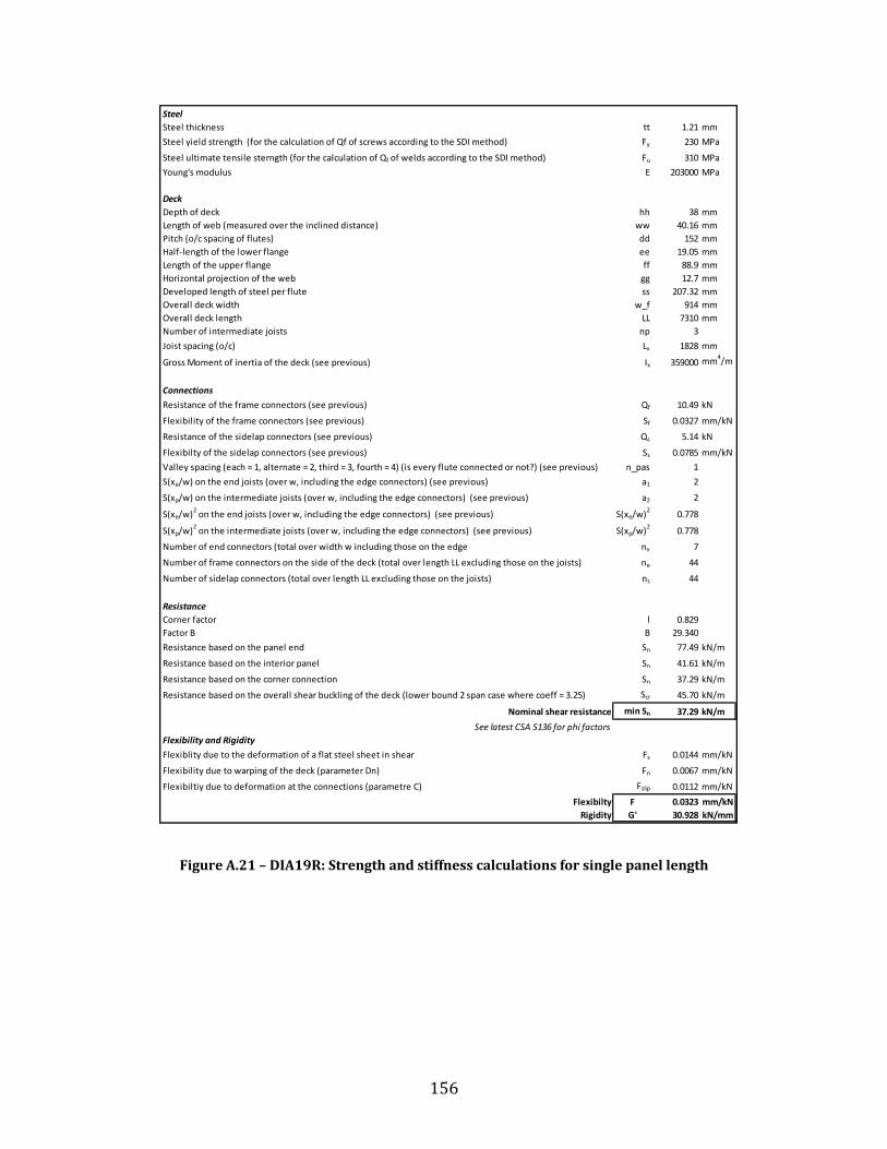
156

Figure A.21 – DIA19R: Strength and stiffness calculations for single panel length

SteelSteel thickness tt 1.21 mm

Steel yield strength (for the calculation of Qf of screws according to the SDI method) Fy 230 MPa

Steel ultimate tensile sterngth (for the calculation of Qf of welds according to the SDI method) Fu 310 MPa

Young's modulus E 203000 MPa

DeckDepth of deck hh 38 mmLength of web (measured over the inclined distance) ww 40.16 mmPitch (o/c spacing of flutes) dd 152 mmHalf-length of the lower flange ee 19.05 mmLength of the upper flange ff 88.9 mmHorizontal projection of the web gg 12.7 mmDeveloped length of steel per flute ss 207.32 mmOverall deck width w_f 914 mmOverall deck length LL 7310 mmNumber of intermediate joists np 3

Joist spacing (o/c) Lv 1828 mm

Gross Moment of inertia of the deck (see previous) Ix 359000 mm4/m

Connections

Resistance of the frame connectors (see previous) Qf 10.49 kN

Flexibility of the frame connectors (see previous) Sf 0.0327 mm/kN

Resistance of the sidelap connectors (see previous) Qs 5.14 kN

Flexibilty of the sidelap connectors (see previous) Ss 0.0785 mm/kN

Valley spacing (each = 1, alternate = 2, third = 3, fourth = 4) (is every flute connected or not?) (see previous) n_pas 1

S(xe/w) on the end joists (over w, including the edge connectors) (see previous) a1 2

S(xp/w) on the intermediate joists (over w, including the edge connectors) (see previous) a2 2

S(xe/w)2 on the end joists (over w, including the edge connectors) (see previous) S(xe/w)2 0.778

S(xp/w)2 on the intermediate joists (over w, including the edge connectors) (see previous) S(xp/w)2 0.778

Number of end connectors (total over width w including those on the edge nv 7

Number of frame connectors on the side of the deck (total over length LL excluding those on the joists) ne 44

Number of sidelap connectors (total over length LL excluding those on the joists) ns 44

ResistanceCorner factor l 0.829Factor B B 29.340

Resistance based on the panel end Sn 77.49 kN/m

Resistance based on the interior panel Sn 41.61 kN/m

Resistance based on the corner connection Sn 37.29 kN/m

Resistance based on the overall shear buckling of the deck (lower bound 2 span case where coeff = 3.25) Scr 45.70 kN/m

Nominal shear resistance min Sn 37.29 kN/m

See latest CSA S136 for phi factorsFlexibility and Rigidity

Flexiblity due to the deformation of a flat steel sheet in shear Fs 0.0144 mm/kN

Flexibility due to warping of the deck (parameter Dn) Fn 0.0067 mm/kN

Flexibiltiy due to deformation at the connections (parametre C) Fslip 0.0112 mm/kN

Flexibilty F 0.0323 mm/kNRigidity G' 30.928 kN/mm

157

Appendix B:

TESTING PROTOCOL CHECKLIST

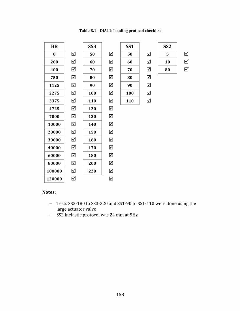
158

Table B.1 – DIA11: Loading protocol checklist BB SS3 SS1 SS2

0 50 50 5

200 60 60 10 400 70 70 80 750 80 80

1125 90 90 2275 100 100 3375 110 110 4725 120 7000 130

10000 140 20000 150 30000 160 40000 170 60000 180 80000 200

100000 220 120000

Notes:

− Tests SS3-180 to SS3-220 and SS1-90 to SS1-110 were done using the large actuator valve − SS2 inelastic protocol was 24 mm at 5Hz

159

Table B.2 – DIA12: Loading protocol checklist BB SS3 SS1 SS2

0 50 50 5

400 60 60 10 1125 80 92 2200 100 3700 120 5175 140 5900 160 8150

10000 20000 30000 40000 60000 80000

100000 120000 140000 160000 180000

Notes:

− SS2 inelastic protocol was 27.6 mm at 5Hz

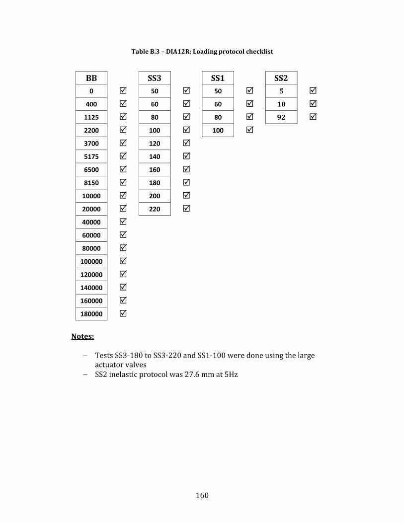
160

Table B.3 – DIA12R: Loading protocol checklist BB SS3 SS1 SS2

0 50 50 5

400 60 60 10 1125 80 80 92 2200 100 100 3700 120 5175 140 6500 160 8150 180

10000 200 20000 220 40000 60000 80000

100000 120000 140000 160000 180000

Notes:

− Tests SS3-180 to SS3-220 and SS1-100 were done using the large actuator valves − SS2 inelastic protocol was 27.6 mm at 5Hz

161

Table B.4 – DIA13: Loading protocol checklist BB SS3 SS1 SS2

0 50 50 2

400 60 60 3 1125 80 80 100 2200 100 100 3700 120 120 5175 140 5900 160 8150 180

10000 200 20000 220 40000 240 60000 280 80000

100000 120000 140000 160000 180000 200000

Notes:

− Tests SS3-180 to SS3-280 and SS1-100 to SS1-120 were done using the large actuator valves − SS2 inelastic protocol was 27.6 mm at 5Hz

162

Table B.5 – DIA13R: Loading protocol checklist BB SS3 SS1 SS2

0 50 50 2

400 60 60 3 1125 80 80 92 2200 100 100 3700 120 5175 140 6500 160 8150 180

10000 200 20000 220 40000 240 60000 80000

100000 120000 140000 160000 180000 200000

Notes:

− Tests SS3-180 to SS3-240 and SS1-100 were done using the large actuator valves − SS2 inelastic protocol was 27.6 mm at 5.25Hz

163

Table B.6 – DIA14: Loading protocol checklist BB SS3 SS1 SS2

0 50 50 5

575 60 60 10 1050 80 80 92 2100 100 100 3200 120 4500 140 6400 160 8550 180

10000 200 12000 220 20000 240 40000 60000 80000

100000 120000

Notes:

− Tests SS3-180 to SS3-240 and SS1-100 were done using the large actuator valves − SS2 inelastic protocol was 27.6 mm at 5.25Hz

164

Table B.7 – DIA15: Loading protocol checklist BB BF SS3 SS1 SS2

0 4.0 50 50 3

150 4.2 60 60 80 225 4.4 80 70 475 4.6 100 80 925 4.8 120

1700 5.0 140 2500 5.1 160 3200 5.2 5050 5.3 8000 5.4

10000 5.5 15000 5.6 20000 5.7 30000 5.8 40000 5.9 60000 6.0 80000

100000

Notes:

− SS2 inelastic protocol was 24 mm at 4Hz

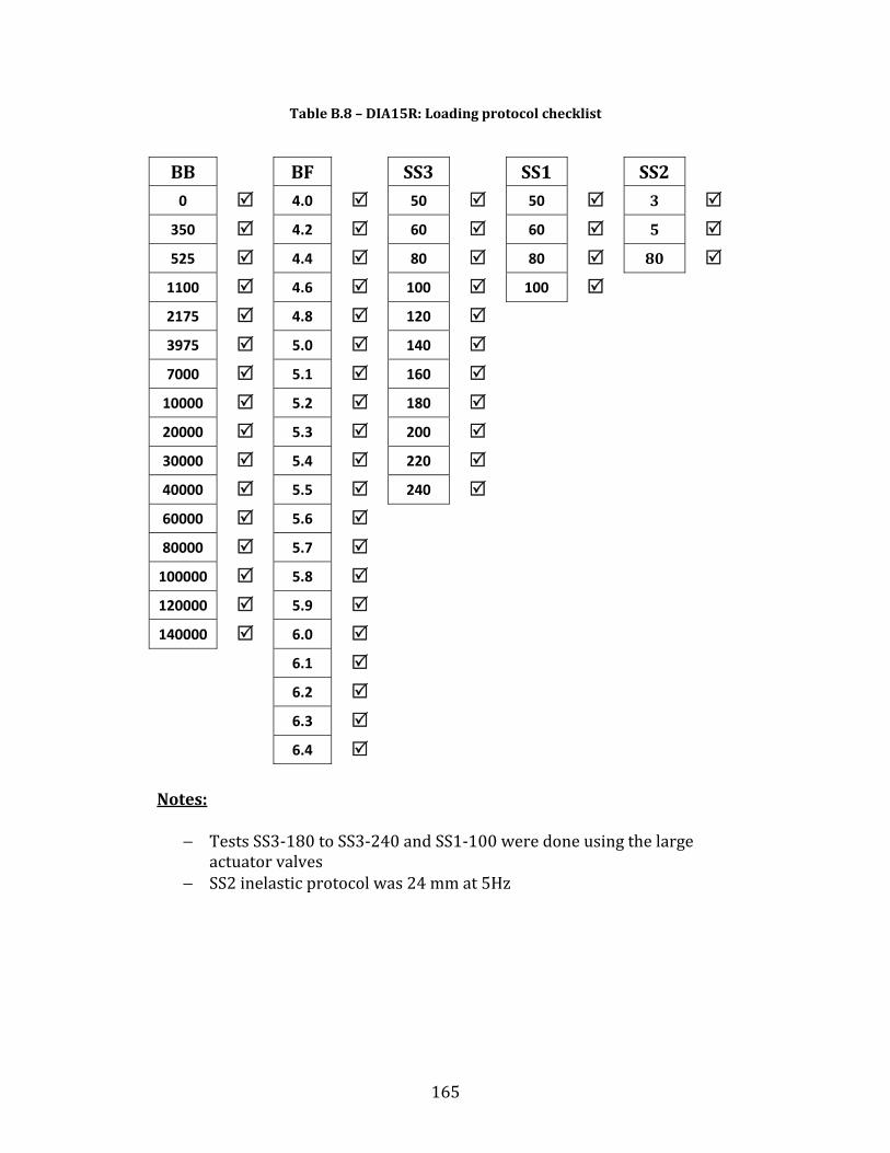
165

Table B.8 – DIA15R: Loading protocol checklist BB BF SS3 SS1 SS2

0 4.0 50 50 3

350 4.2 60 60 5 525 4.4 80 80 80

1100 4.6 100 100 2175 4.8 120 3975 5.0 140 7000 5.1 160

10000 5.2 180 20000 5.3 200 30000 5.4 220 40000 5.5 240 60000 5.6 80000 5.7

100000 5.8 120000 5.9 140000 6.0

6.1 6.2 6.3 6.4

Notes:

− Tests SS3-180 to SS3-240 and SS1-100 were done using the large actuator valves − SS2 inelastic protocol was 24 mm at 5Hz

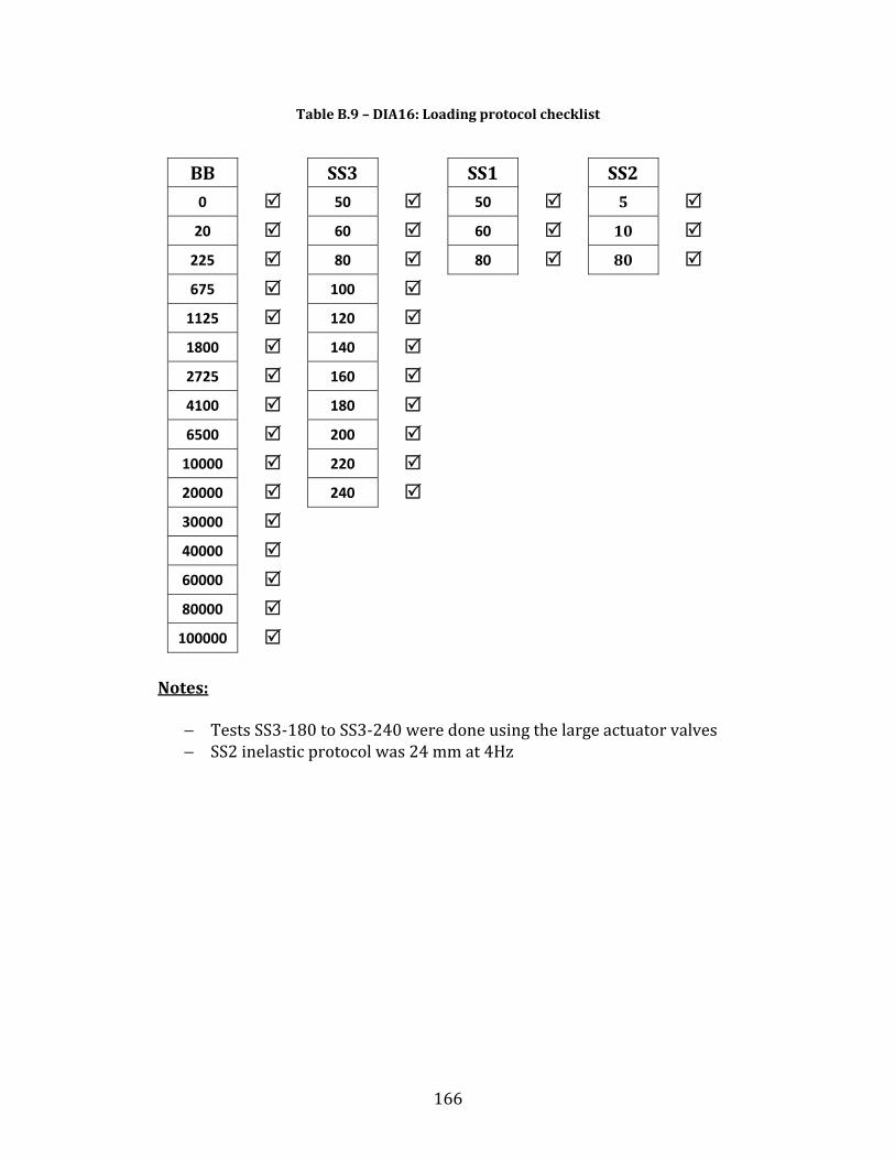
166

Table B.9 – DIA16: Loading protocol checklist BB SS3 SS1 SS2

0 50 50 5

20 60 60 10 225 80 80 80 675 100

1125 120 1800 140 2725 160 4100 180 6500 200

10000 220 20000 240 30000 40000 60000 80000

100000

Notes:

− Tests SS3-180 to SS3-240 were done using the large actuator valves − SS2 inelastic protocol was 24 mm at 4Hz

167

Table B.10 – DIA16R: Loading protocol checklist BB SS3 SS1 SS2

0 50 50 5

225 60 60 10 675 80 80 80

1125 100 100 1800 120 120 2725 140 140 4100 160 6500 180

10000 200 20000 220 30000 240 40000 260 60000 280 80000

100000 120000 160000

Notes:

− Tests SS3-180 to SS3-280 and SS1-100 to SS1-140 were done using the large actuator valves − SS2 inelastic protocol was 24 mm at 5Hz

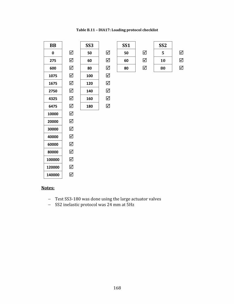
168

Table B.11 – DIA17: Loading protocol checklist BB SS3 SS1 SS2

0 50 50 5

275 60 60 10 600 80 80 80

1075 100 1675 120 2750 140 4325 160 6475 180

10000 20000 30000 40000 60000 80000

100000 120000 140000

Notes:

− Test SS3-180 was done using the large actuator valves − SS2 inelastic protocol was 24 mm at 5Hz

169

Table B.12 – DIA17R: Loading protocol checklist BB SS3 SS1 SS2

0 50 50 5

275 60 60 10 600 80 80 80

1075 100 100 1675 120 120 2750 140 140 4325 160 6475 180

10000 200 20000 220 30000 40000 60000 80000

100000 120000 140000

Notes:

− Tests SS3-180 to SS3-220 and SS1-100 to SS1-140 were done using the large actuator valves − SS2 inelastic protocol was 24 mm at 5Hz

170

Table B.13 – DIA18: Loading protocol checklist BB SS3 SS1 SS2

0 50 50 5

150 60 60 5.75 325 80 80 10 750 100 100 92

1325 120 2175 140 3400 160 4675 180 6100 8000

10000 20000 30000 40000

Notes:

− Tests SS3-180 and SS1-100 were done using the large actuator valves − SS2 inelastic protocol was 27.6 mm at 5Hz

171

Table B.14 – DIA18R: Loading protocol checklist BB SS3 SS1 SS2

0 50 50 5

150 60 60 10 325 80 80 92 750 100 100

1325 120 120 2175 140 3400 160 4675 180 6100 200 8000 220

10000 240 20000 260 30000 280 40000 60000 80000

100000 120000 140000 160000 180000

Notes:

− Tests SS3-180 to SS3-280 and SS1-100 to SS1-120 were done using the large actuator valves − SS2 inelastic protocol was 27.6 mm at 5Hz

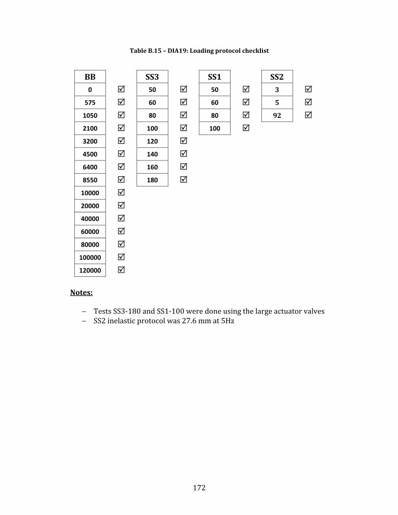
172

Table B.15 – DIA19: Loading protocol checklist BB SS3 SS1 SS2

0 50 50 3

575 60 60 5 1050 80 80 92 2100 100 100 3200 120 4500 140 6400 160 8550 180

10000 20000 40000 60000 80000

100000 120000

Notes:

− Tests SS3-180 and SS1-100 were done using the large actuator valves − SS2 inelastic protocol was 27.6 mm at 5Hz

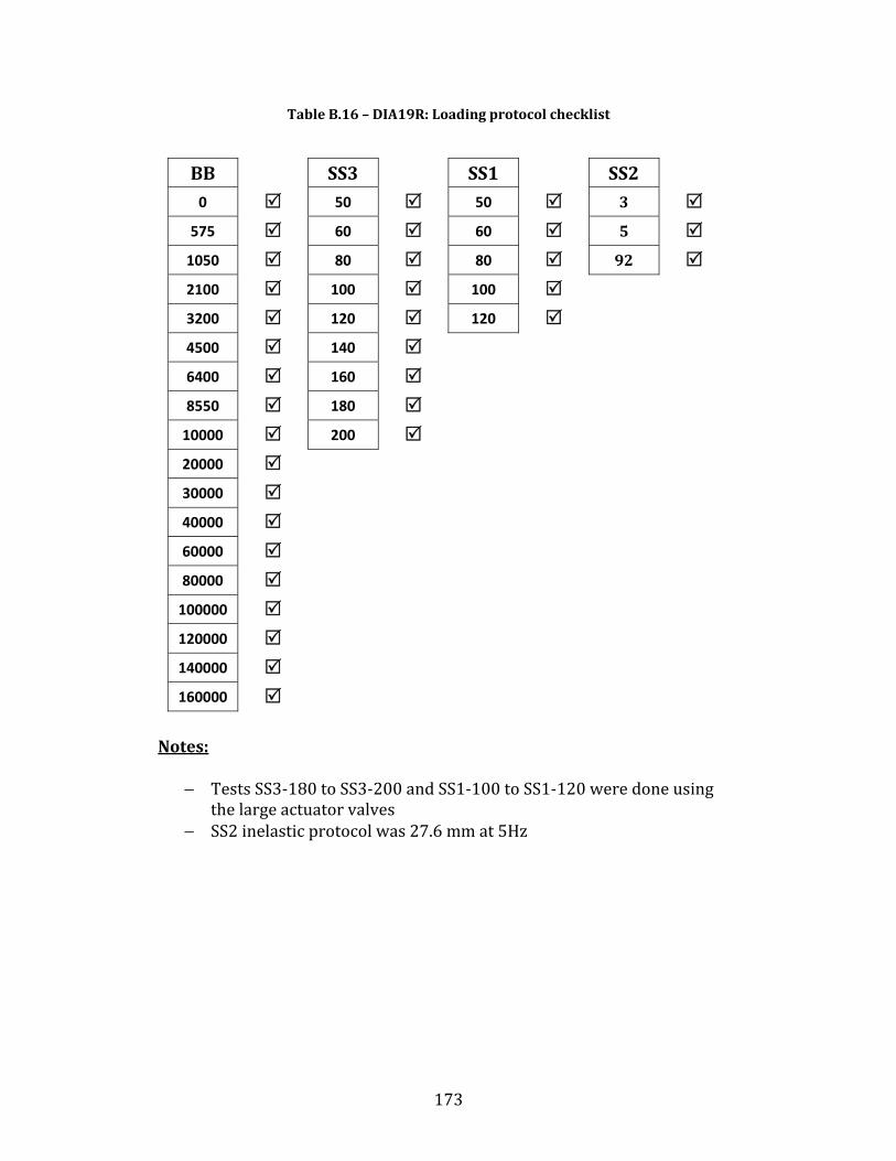
173

Table B.16 – DIA19R: Loading protocol checklist BB SS3 SS1 SS2

0 50 50 3

575 60 60 5 1050 80 80 92 2100 100 100 3200 120 120 4500 140 6400 160 8550 180

10000 200 20000 30000 40000 60000 80000

100000 120000 140000 160000

Notes:

− Tests SS3-180 to SS3-200 and SS1-100 to SS1-120 were done using the large actuator valves − SS2 inelastic protocol was 27.6 mm at 5Hz

174

Appendix C:

FREQUENCY RESULTS FROM WHITE NOISE TESTING

FOR NEW DIAPHRAGM SPECIMENS

175

Figure C.1 – DIA11: Fundamental period as a function of the root mean square of the

response acceleration

Figure C.2 – DIA11: Comparison of experimental and predicted stiffness at varying

levels of the predicted strength

0 500 1000 1500 2000RMS Absolute Acceleration (mm/s2)

0.00

0.05

0.10

0.15

0.20

Fund

amen

tal P

erio

d (s

)

DIA11 ResultsLog Fit DIA11TMedhekar (G' = 11.6 kN/mm)

0.0 0.2 0.4 0.6S/Sn

0.00

0.50

1.00

1.50

2.00

G' ex

perim

enta

l/G' SD

I

DIA11 ResultsLog Fit DIA11G' = G'SDI

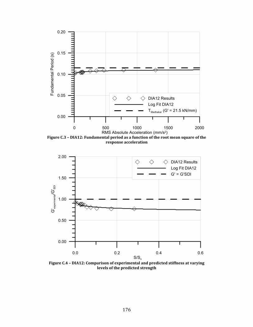
176

Figure C.3 – DIA12: Fundamental period as a function of the root mean square of the

response acceleration

Figure C.4 – DIA12: Comparison of experimental and predicted stiffness at varying

levels of the predicted strength

0 500 1000 1500 2000RMS Absolute Acceleration (mm/s2)

0.00

0.05

0.10

0.15

0.20

Fund

amen

tal P

erio

d (s

)

DIA12 ResultsLog Fit DIA12TMedhekar (G' = 21.5 kN/mm)

0.0 0.2 0.4 0.6S/Sn

0.00

0.50

1.00

1.50

2.00

G' ex

perim

enta

l/G' SD

I

DIA12 ResultsLog Fit DIA12G' = G'SDI

177

Figure C.5 – DIA13: Fundamental period as a function of the root mean square of the

response acceleration

Figure C.6 – DIA13: Comparison of experimental and predicted stiffness at varying

levels of the predicted strength

0 500 1000 1500 2000RMS Absolute Acceleration (mm/s2)

0.00

0.05

0.10

0.15

0.20

Fund

amen

tal P

erio

d (s

)

DIA13 ResultsLog Fit DIA13TMedhekar (G' = 25.6 kN/mm)

0.0 0.2 0.4 0.6S/Sn

0.00

0.50

1.00

1.50

2.00

G' ex

perim

enta

l/G' SD

I

DIA13 ResultsLog Fit DIA13G' = G'SDI

178

Figure C.7 – DIA14: Fundamental period as a function of the root mean square of the

response acceleration

Figure C.8 – DIA14: Comparison of experimental and predicted stiffness at varying

levels of the predicted strength

0 500 1000 1500 2000RMS Absolute Acceleration (mm/s2)

0.00

0.05

0.10

0.15

0.20

Fund

amen

tal P

erio

d (s

)

DIA14 ResultsLog Fit DIA14TMedhekar (G' = 23.4 kN/mm)

0.0 0.2 0.4 0.6S/Sn

0.00

0.50

1.00

1.50

2.00

G' ex

perim

enta

l/G' SD

I

DIA14 ResultsLog Fit DIA14G' = G'SDI

179

Figure C.9 – DIA15: Fundamental period as a function of the root mean square of the

response acceleration

Figure C.10 – DIA15: Comparison of experimental and predicted stiffness at varying

levels of the predicted strength

0 500 1000RMS Absolute Acceleration (mm/s2)

0.00

0.05

0.10

0.15

0.20

0.25

0.30

Fund

amen

tal P

erio

d (s

)

DIA15 ResultsLog Fit DIA15TMedhekar (G' = 3.5 kN/mm)

0.0 0.2 0.4 0.6S/Sn

0.00

1.00

2.00

3.00

4.00

5.00

G' ex

perim

enta

l/G' SD

I

DIA15 ResultsLog Fit DIA15G' = G'SDI

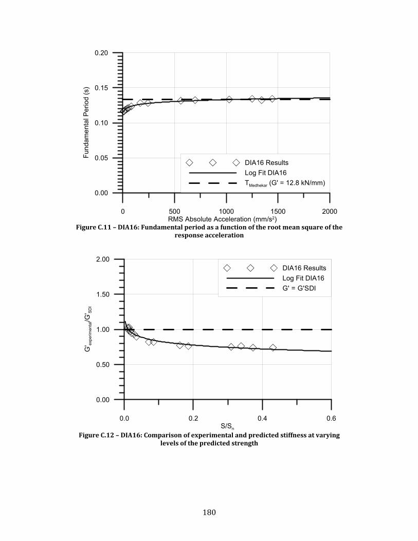
180

Figure C.11 – DIA16: Fundamental period as a function of the root mean square of the

response acceleration

Figure C.12 – DIA16: Comparison of experimental and predicted stiffness at varying

levels of the predicted strength

0 500 1000 1500 2000RMS Absolute Acceleration (mm/s2)

0.00

0.05

0.10

0.15

0.20

Fund

amen

tal P

erio

d (s

)

DIA16 ResultsLog Fit DIA16TMedhekar (G' = 12.8 kN/mm)

0.0 0.2 0.4 0.6S/Sn

0.00

0.50

1.00

1.50

2.00

G' ex

perim

enta

l/G' SD

I

DIA16 ResultsLog Fit DIA16G' = G'SDI

181

Figure C.13 – DIA17: Fundamental period as a function of the root mean square of the

response acceleration

Figure C.14 – DIA17: Comparison of experimental and predicted stiffness at varying

levels of the predicted strength

0 500 1000 1500 2000RMS Absolute Acceleration (mm/s2)

0.00

0.05

0.10

0.15

0.20

Fund

amen

tal P

erio

d (s

)

DIA17 ResultsLog Fit DIA17TMedhekar (G' = 14.1 kN/mm)

0.0 0.2 0.4 0.6S/Sn

0.00

0.50

1.00

1.50

2.00

G' ex

perim

enta

l/G' SD

I

DIA17 ResultsLog Fit DIA17G' = G'SDI

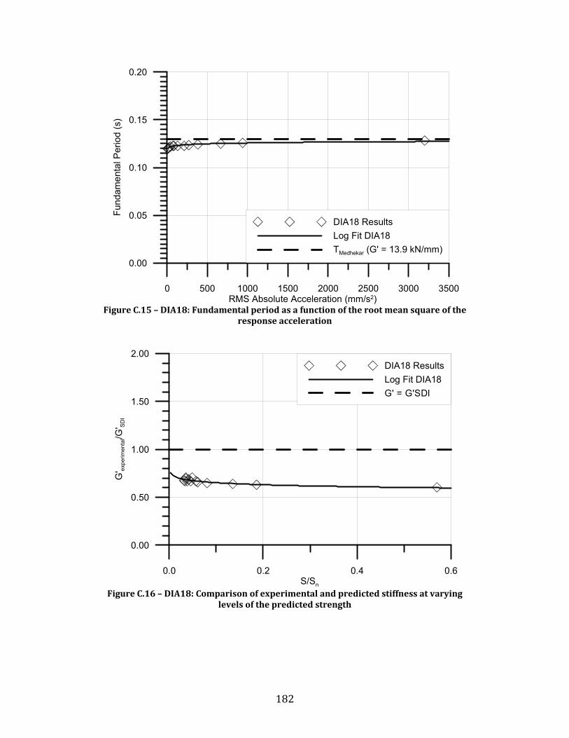
182

Figure C.15 – DIA18: Fundamental period as a function of the root mean square of the

response acceleration

Figure C.16 – DIA18: Comparison of experimental and predicted stiffness at varying

levels of the predicted strength

0 500 1000 1500 2000 2500 3000 3500RMS Absolute Acceleration (mm/s2)

0.00

0.05

0.10

0.15

0.20

Fund

amen

tal P

erio

d (s

)

DIA18 ResultsLog Fit DIA18TMedhekar (G' = 13.9 kN/mm)

0.0 0.2 0.4 0.6S/Sn

0.00

0.50

1.00

1.50

2.00

G' ex

perim

enta

l/G' SD

I

DIA18 ResultsLog Fit DIA18G' = G'SDI

183

Figure C.17 – DIA19: Fundamental period as a function of the root mean square of the

response acceleration

Figure C.18 – DIA19: Comparison of experimental and predicted stiffness at varying

levels of the predicted strength

0 500 1000 1500 2000RMS Absolute Acceleration (mm/s2)

0.00

0.05

0.10

0.15

0.20

Fund

amen

tal P

erio

d (s

)

DIA19 ResultsLog Fit DIA19TMedhekar (G' = 18.7 kN/mm)

0.0 0.2 0.4 0.6S/Sn

0.00

0.50

1.00

1.50

2.00

G' ex

perim

enta

l/G' SD

I

DIA19 ResultsLog Fit DIA19G' = G'SDI

184

Appendix D:

FREQUENCY RESULTS FROM WHITE NOISE TESTING

FOR REPAIRED DIAPHRAGM SPECIMENS

185

Figure D.1 – DIA12R: Fundamental period as a function of the root mean square of the

response acceleration

Figure D.2 – DIA12R: Comparison of experimental and predicted stiffness at varying

levels of the predicted strength

0 500 1000 1500 2000RMS Absolute Acceleration (mm/s2)

0.00

0.05

0.10

0.15

0.20

Fund

amen

tal P

erio

d (s

)

DIA12R ResultsLog Fit DIA12RTMedhekar (G' = 20.2 kN/mm)

0.0 0.2 0.4 0.6qmax/qSDI

0.00

0.50

1.00

1.50

2.00

G' ex

perim

enta

l/G' SD

I

DIA12R ResultsLog Fit DIA12RG' = G'SDI

186

Figure D.3 – DIA13R: Fundamental period as a function of the root mean square of the

response acceleration

Figure D.4 – DIA13R: Comparison of experimental and predicted stiffness at varying

levels of the predicted strength

0 500 1000 1500 2000RMS Absolute Acceleration (mm/s2)

0.00

0.05

0.10

0.15

0.20

Fund

amen

tal P

erio

d (s

)

DIA13R ResultsLog Fit DIA13RTMedhekar (G' = 22.9 kN/mm)

0.0 0.2 0.4 0.6S/Sn

0.00

0.50

1.00

1.50

2.00

G' ex

perim

enta

l/G' SD

I

DIA13R ResultsLog Fit DIA13RG' = G'SDI

187

Figure D.5 – DIA15R: Fundamental period as a function of the root mean square of the

response acceleration

Figure D.6 – DIA15R: Comparison of experimental and predicted stiffness at varying

levels of the predicted strength

0 500 1000RMS Absolute Acceleration (mm/s2)

0.00

0.05

0.10

0.15

0.20

0.25

0.30

0.35

Fund

amen

tal P

erio

d (s

)

DIA15R ResultsLog Fit DIA15RTMedhekar (G' = 2.6 kN/mm)

0.0 0.2 0.4 0.6S/Sn

0.00

1.00

2.00

3.00

4.00

5.00

G' ex

perim

enta

l/G' SD

I

DIA15R ResultsLog Fit DIA15RG' = G'SDI

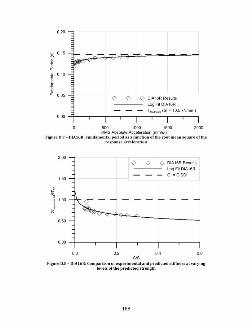
188

Figure D.7 – DIA16R: Fundamental period as a function of the root mean square of the

response acceleration

Figure D.8 – DIA16R: Comparison of experimental and predicted stiffness at varying

levels of the predicted strength

0 500 1000 1500 2000RMS Absolute Acceleration (mm/s2)

0.00

0.05

0.10

0.15

0.20

Fund

amen

tal P

erio

d (s

)

DIA16R ResultsLog Fit DIA16RTMedhekar (G' = 10.5 kN/mm)

0.0 0.2 0.4 0.6S/Sn

0.00

0.50

1.00

1.50

2.00

G' ex

perim

enta

l/G' SD

I

DIA16R ResultsLog Fit DIA16RG' = G'SDI

189

Figure D.9 – DIA17R: Fundamental period as a function of the root mean square of the

response acceleration

Figure D.10 – DIA17R: Comparison of experimental and predicted stiffness at varying

levels of the predicted strength

0 500 1000 1500 2000RMS Absolute Acceleration (mm/s2)

0.00

0.05

0.10

0.15

0.20

Fund

amen

tal P

erio

d (s

)

DIA17R ResultsLog Fit DIA17RTMedhekar (G' = 9.4 kN/mm)

0.0 0.2 0.4 0.6S/Sn

0.00

0.50

1.00

1.50

2.00

G' ex

perim

enta

l/G' SD

I

DIA17R ResultsLog Fit DIA17RG' = G'SDI

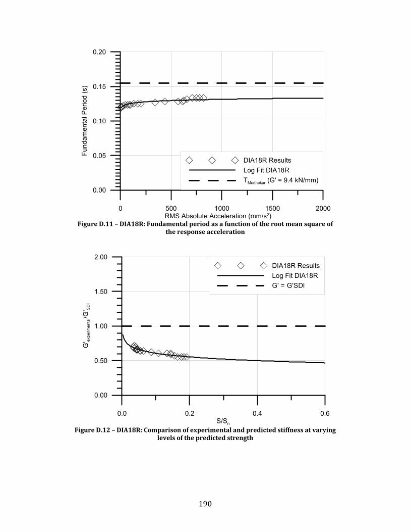
190

Figure D.11 – DIA18R: Fundamental period as a function of the root mean square of

the response acceleration

Figure D.12 – DIA18R: Comparison of experimental and predicted stiffness at varying

levels of the predicted strength

0 500 1000 1500 2000RMS Absolute Acceleration (mm/s2)

0.00

0.05

0.10

0.15

0.20

Fund

amen

tal P

erio

d (s

)

DIA18R ResultsLog Fit DIA18RTMedhekar (G' = 9.4 kN/mm)

0.0 0.2 0.4 0.6S/Sn

0.00

0.50

1.00

1.50

2.00

G' ex

perim

enta

l/G' SD

I

DIA18R ResultsLog Fit DIA18RG' = G'SDI

191

Figure D.13 – DIA19R: Fundamental period as a function of the root mean square of

the response acceleration

Figure D.14 – DIA19R: Comparison of experimental and predicted stiffness at varying

levels of the predicted strength

0 500 1000 1500 2000RMS Absolute Acceleration (mm/s2)

0.00

0.05

0.10

0.15

0.20

Fund

amen

tal P

erio

d (s

)

DIA19R ResultsLog Fit DIA19RTMedhekar (G' = 16.6 kN/mm)

0.0 0.2 0.4 0.6S/Sn

0.00

0.50

1.00

1.50

2.00

G' ex

perim

enta

l/G' SD

I

DIA19R ResultsLog Fit DIA19RG' = G'SDI

192

Appendix E:

DAMPING RATIOS

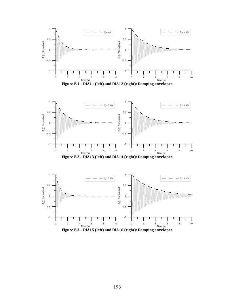
193

Figure E.1 – DIA11 (left) and DIA12 (right): Damping envelopes

Figure E.2 – DIA13 (left) and DIA14 (right): Damping envelopes

Figure E.3 – DIA15 (left) and DIA16 (right): Damping envelopes

0 2 4 6 8 10Time (s)

-1

-0.5

0

0.5

1

R1(

t) N

orm

aliz

ed

ζ = 4%

0 2 4 6 8 10Time (s)

-1

-0.5

0

0.5

1

R1(

t) N

orm

aliz

ed

ζ = 1.8%

0 2 4 6 8 10Time (s)

-1

-0.5

0

0.5

1

R1(

t) N

orm

aliz

ed

ζ = 2.4%

0 2 4 6 8 10Time (s)

-1

-0.5

0

0.5

1

R1(

t) N

orm

aliz

ed

ζ = 1.9%

0 2 4 6 8 10Time (s)

-1

-0.5

0

0.5

1

R1(

t) N

orm

aliz

ed

ζ = 5.3%

0 2 4 6 8 10Time (s)

-1

-0.5

0

0.5

1

R1(

t) N

orm

aliz

ed

ζ = 1.1%

194

Figure E.4 – DIA17 (left) and DIA18 (right): Damping envelopes

Figure E.5 – DIA19: Damping envelope

0 2 4 6 8 10Time (s)

-1

-0.5

0

0.5

1

R1(

t) N

orm

aliz

ed

ζ = 0.8%

0 2 4 6 8 10Time (s)

-1

-0.5

0

0.5

1

R1(

t) N

orm

aliz

ed

ζ = 1.1%

0 2 4 6 8 10Time (s)

-1

-0.5

0

0.5

1

R1(

t) N

orm

aliz

ed

ζ = 1.8%

195

Appendix F:

SINE SWEEP RESONANCE CURVES

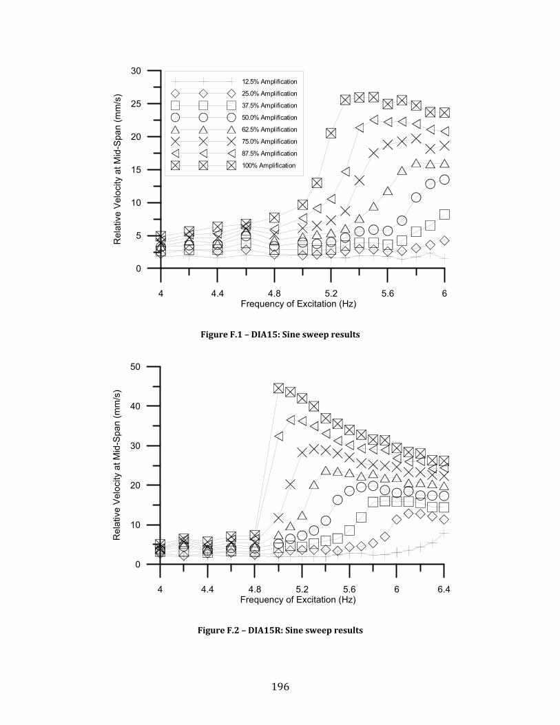
196

Figure F.1 – DIA15: Sine sweep results

Figure F.2 – DIA15R: Sine sweep results

4 4.4 4.8 5.2 5.6 6Frequency of Excitation (Hz)

0

5

10

15

20

25

30

Rel

ativ

e Ve

loci

ty a

t Mid

-Spa

n (m

m/s

)

12.5% Amplification

25.0% Amplification

37.5% Amplification

50.0% Amplification

62.5% Amplification

75.0% Amplification

87.5% Amplification

100% Amplification

4 4.4 4.8 5.2 5.6 6 6.4Frequency of Excitation (Hz)

0

10

20

30

40

50

Rel

ativ

e Ve

loci

ty a

t Mid

-Spa

n (m

m/s

)

197

Appendix G:

SHEAR FORCE AND DEFORMATION PROFILES FOR

NEW DIAPHRAGM SPECIMENS

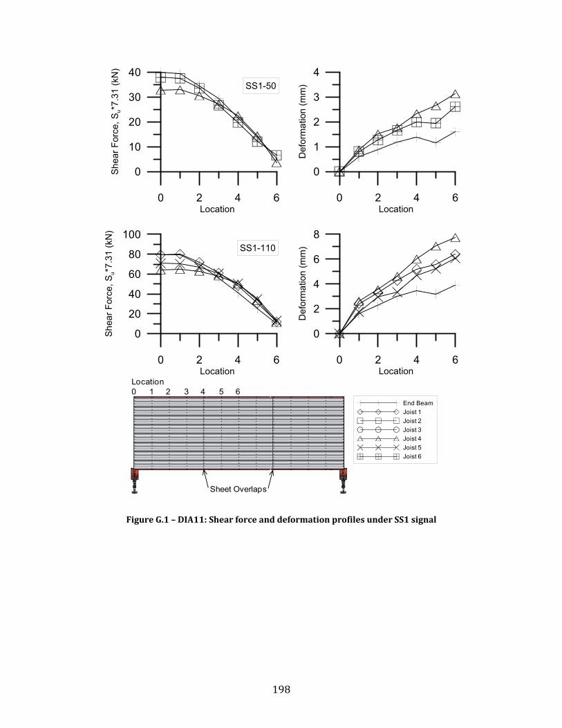
198

Figure G.1 – DIA11: Shear force and deformation profiles under SS1 signal

0 2 4 6Location

0

20

40

60

80

100

Shea

r For

ce, S

u*7.

31 (k

N)

SS1-110

0 2 4 6Location

0

1

2

3

4

Def

orm

atio

n (m

m)

0 2 4 6Location

0

2

4

6

8

Def

orm

atio

n (m

m)

0 2 4 6Location

0

10

20

30

40

Shea

r For

ce, S

u*7.

31 (k

N)

SS1-50

Sheet Overlaps

Location0 1 2 3 4 5 6

End BeamJoist 1Joist 2Joist 3Joist 4Joist 5Joist 6

199

Figure G.2 – DIA11: Shear force and deformation profiles under SS3 and SS2 signals

0 2 4 6Location

0

4

8

12

16

20

Shea

r For

ce, S

u*7.

31 (k

N)

SS3-50

0 2 4 6Location

0

20

40

60

80

She

ar F

orce

, Su*

7.31

(kN

)

SS3-240

0 2 4 6Location

0

40

80

120

160

200

Shea

r For

ce, S

u*7.

31 (k

N)

SS2-80

0 2 4 6Location

0

0.4

0.8

1.2

Def

orm

atio

n (m

m)

0 2 4 6Location

0

2

4

6

8

Def

orm

atio

n (m

m)

0 2 4 6Location

0

10

20

30

40

Def

orm

atio

n (m

m)

Sheet Overlaps

Location0 1 2 3 4 5 6

End BeamJoist 1Joist 2Joist 3Joist 4Joist 5Joist 6

200

Figure G.3 – DIA12: Shear force and deformation profiles under SS1 signal

0 2 4 6Location

0

10

20

30

40

Shea

r For

ce, S

u*7.

31 (k

N)

SS1-60

0 2 4 6Location

0

0.4

0.8

1.2

Def

orm

atio

n (m

m)

0 2 4 6Location

0

0.4

0.8

1.2

1.6

Def

orm

atio

n (m

m)

0 2 4 6Location

0

10

20

30

40

Shea

r For

ce, S

u*7.

31 (k

N)

SS1-50

Sheet Overlaps

Location0 1 2 3 4 5 6

End BeamJoist 1Joist 2Joist 3Joist 4Joist 5Joist 6

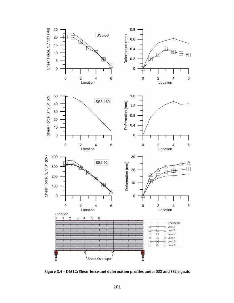
201

Figure G.4 – DIA12: Shear force and deformation profiles under SS3 and SS2 signals

0 2 4 6Location

0

5

10

15

20

25

Shea

r For

ce, S

u*7.

31 (k

N)

SS3-50

0 2 4 6Location

0

10

20

30

40

50

She

ar F

orce

, Su*

7.31

(kN

)

SS3-160

0 2 4 6Location

0

100

200

300

400

Shea

r For

ce, S

u*7.

31 (k

N)

SS2-92

0 2 4 6Location

0

0.2

0.4

0.6

0.8

Def

orm

atio

n (m

m)

0 2 4 6Location

0

0.4

0.8

1.2

1.6

Def

orm

atio

n (m

m)

0 2 4 6Location

0

10

20

30

Def

orm

atio

n (m

m)

Sheet Overlaps

Location0 1 2 3 4 5 6

End BeamJoist 1Joist 2Joist 3Joist 4Joist 5Joist 6

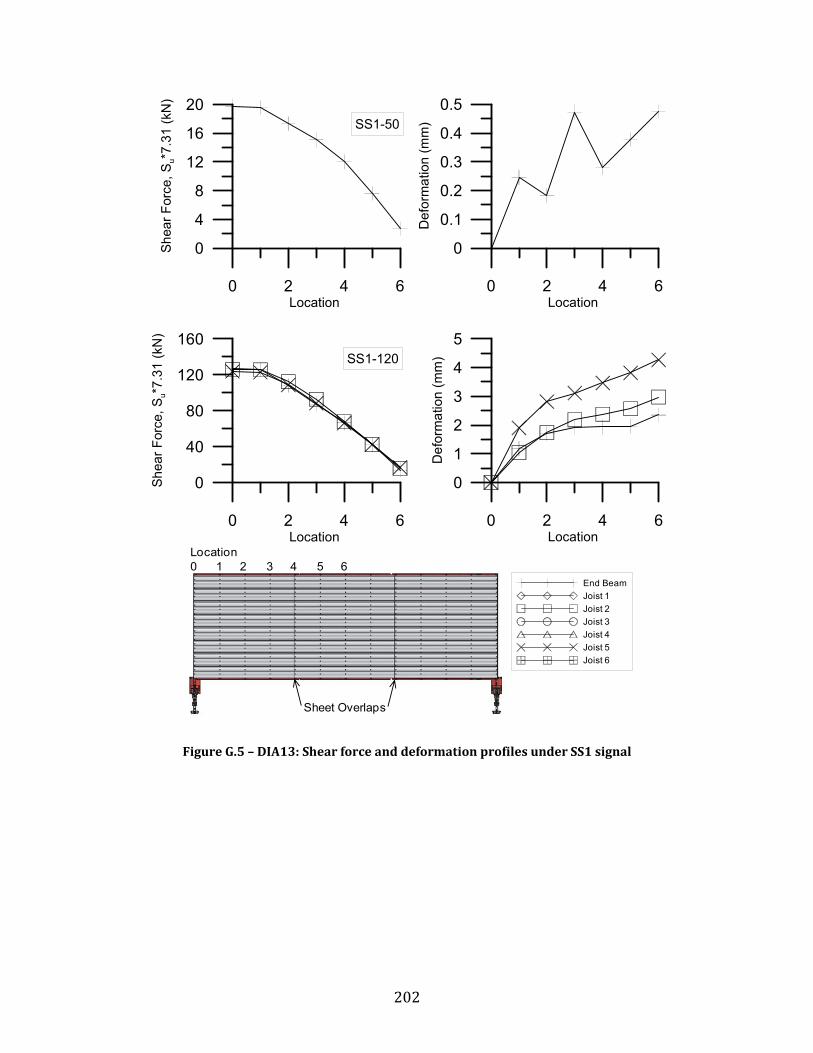
202

Figure G.5 – DIA13: Shear force and deformation profiles under SS1 signal

0 2 4 6Location

0

40

80

120

160

Shea

r For

ce, S

u*7.

31 (k

N)

SS1-120

0 2 4 6Location

0

0.1

0.2

0.3

0.4

0.5

Def

orm

atio

n (m

m)

0 2 4 6Location

0

1

2

3

4

5

Def

orm

atio

n (m

m)

0 2 4 6Location

0

4

8

12

16

20

Shea

r For

ce, S

u*7.

31 (k

N)

SS1-50

Sheet Overlaps

Location0 1 2 3 4 5 6

End BeamJoist 1Joist 2Joist 3Joist 4Joist 5Joist 6

203

Figure G.6 – DIA13: Shear force and deformation profiles under SS3 and SS2 signals

0 2 4 6Location

0

4

8

12

16

Shea

r For

ce, S

u*7.

31 (k

N)

SS3-50

0 2 4 6Location

0

40

80

120

She

ar F

orce

, Su*

7.31

(kN

)

SS3-280

0 2 4 6Location

0

200

400

600

Shea

r For

ce, S

u*7.

31 (k

N)

SS2-92

0 2 4 6Location

0

0.1

0.2

0.3

0.4

Def

orm

atio

n (m

m)

0 2 4 6Location

0

1

2

3

4

Def

orm

atio

n (m

m)

0 2 4 6Location

0

5

10

15

20

25

Def

orm

atio

n (m

m)

Sheet Overlaps

Location0 1 2 3 4 5 6

End BeamJoist 1Joist 2Joist 3Joist 4Joist 5Joist 6

204

Figure G.7 – DIA14: Shear force and deformation profiles under SS1 signal

0 2 4 6Location

0

40

80

120

160

200

She

ar F

orce

, Su*

7.31

(kN

)

SS1-100

0 2 4 6Location

0

0.4

0.8

1.2

1.6

Def

orm

atio

n (m

m)

0 2 4 6Location

0

1

2

3

4

5

Def

orm

atio

n (m

m)

0 2 4 6Location

0

10

20

30

40

Shea

r For

ce, S

u*7.

31 (k

N)

SS1-50

Sheet Overlaps

Location0 1 2 3 4 5 6

End BeamJoist 1Joist 2Joist 3Joist 4Joist 5Joist 6

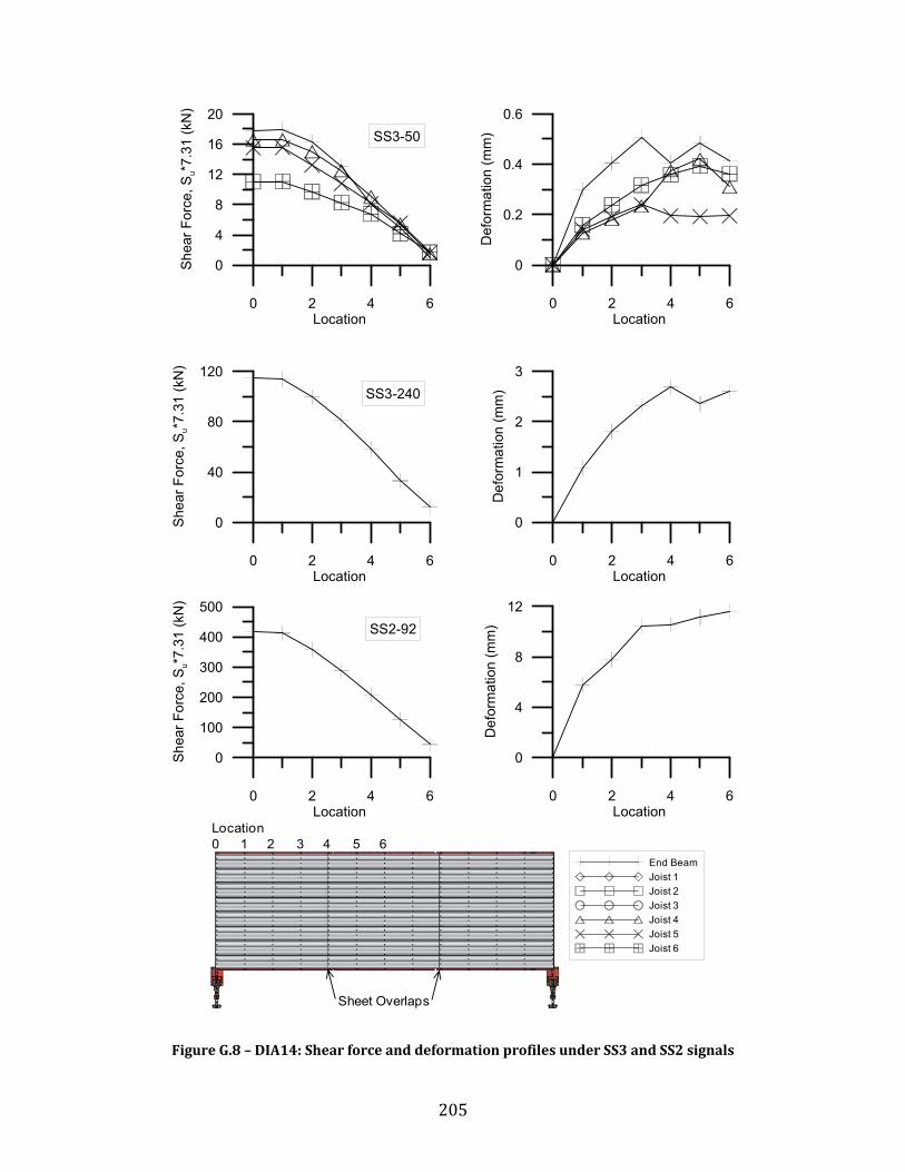
205

Figure G.8 – DIA14: Shear force and deformation profiles under SS3 and SS2 signals

0 2 4 6Location

0

4

8

12

16

20

Shea

r For

ce, S

u*7.

31 (k

N)

SS3-50

0 2 4 6Location

0

40

80

120

She

ar F

orce

, Su*

7.31

(kN

)

SS3-240

0 2 4 6Location

0

100

200

300

400

500

Shea

r For

ce, S

u*7.

31 (k

N)

SS2-92

0 2 4 6Location

0

0.2

0.4

0.6

Def

orm

atio

n (m

m)

0 2 4 6Location

0

1

2

3

Def

orm

atio

n (m

m)

0 2 4 6Location

0

4

8

12

Def

orm

atio

n (m

m)

Sheet Overlaps

Location0 1 2 3 4 5 6

End BeamJoist 1Joist 2Joist 3Joist 4Joist 5Joist 6

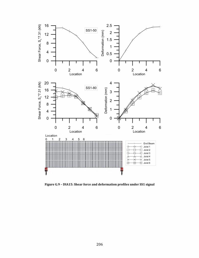
206

Figure G.9 – DIA15: Shear force and deformation profiles under SS1 signal

0 2 4 6Location

0

4

8

12

16

20

Shea

r For

ce, S

u*7.

31 (k

N)

SS1-80

0 2 4 6Location

0

0.5

1

1.5

2

2.5

Def

orm

atio

n (m

m)

0 2 4 6Location

0

1

2

3

4

Def

orm

atio

n (m

m)

0 2 4 6Location

0

4

8

12

16

Shea

r For

ce, S

u*7.

31 (k

N)

SS1-50

Location0 1 2 3 4 5 6

End BeamJoist 1Joist 2Joist 3Joist 4Joist 5Joist 6

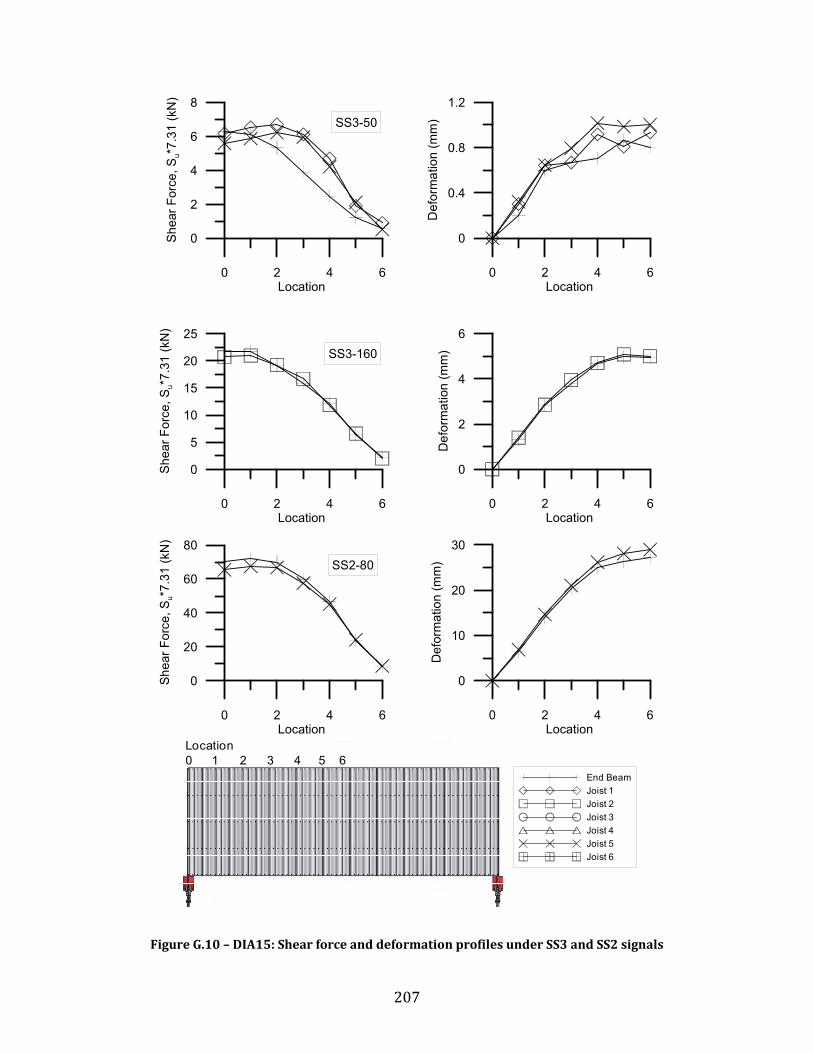
207

Figure G.10 – DIA15: Shear force and deformation profiles under SS3 and SS2 signals

0 2 4 6Location

0

2

4

6

8

Shea

r For

ce, S

u*7.

31 (k

N)

SS3-50

0 2 4 6Location

0

5

10

15

20

25

She

ar F

orce

, Su*

7.31

(kN

)

SS3-160

0 2 4 6Location

0

20

40

60

80

Shea

r For

ce, S

u*7.

31 (k

N)

SS2-80

0 2 4 6Location

0

0.4

0.8

1.2

Def

orm

atio

n (m

m)

0 2 4 6Location

0

2

4

6

Def

orm

atio

n (m

m)

0 2 4 6Location

0

10

20

30

Def

orm

atio

n (m

m)

Location0 1 2 3 4 5 6

End BeamJoist 1Joist 2Joist 3Joist 4Joist 5Joist 6

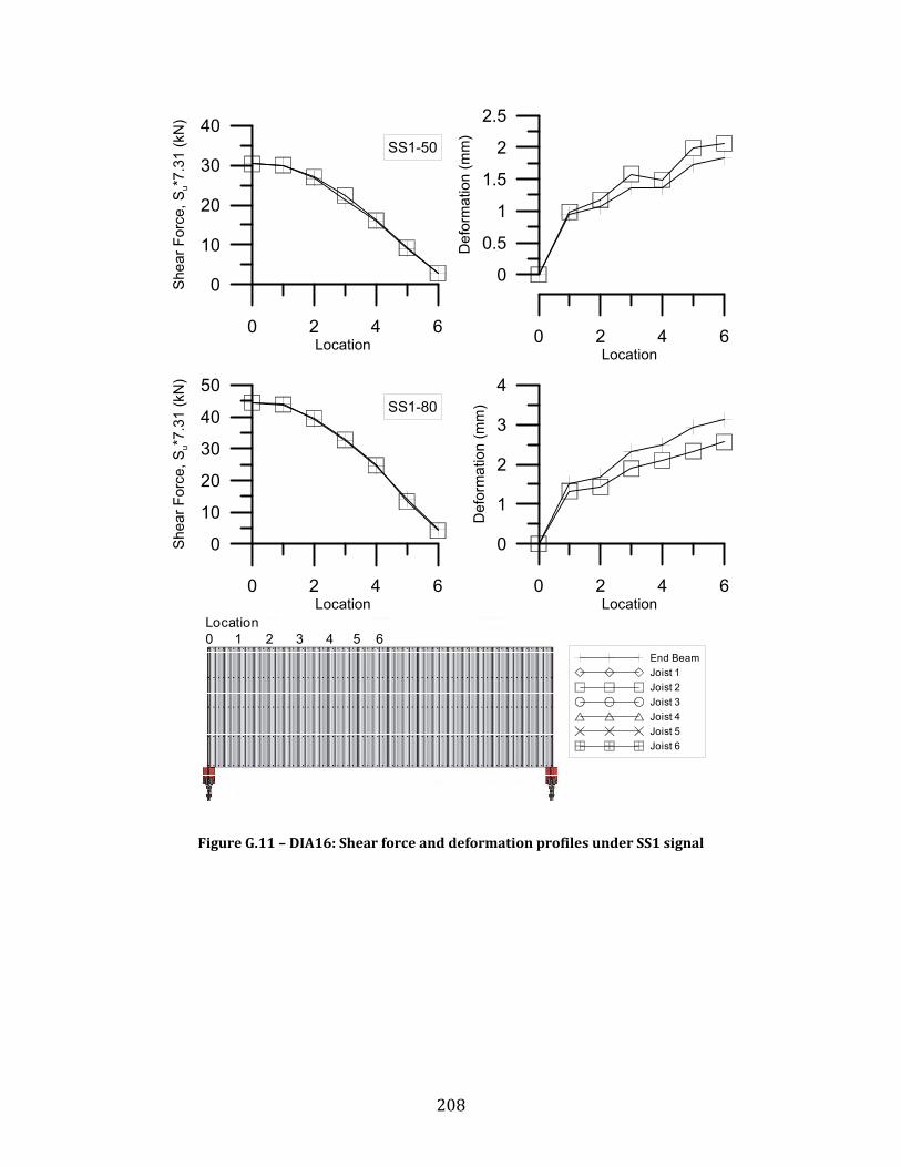
208

Figure G.11 – DIA16: Shear force and deformation profiles under SS1 signal

0 2 4 6Location

0

10

20

30

40

50

She

ar F

orce

, Su*

7.31

(kN

)

SS1-80

0 2 4 6Location

0

0.5

1

1.5

2

2.5

Def

orm

atio

n (m

m)

0 2 4 6Location

0

1

2

3

4

Def

orm

atio

n (m

m)

0 2 4 6Location

0

10

20

30

40

She

ar F

orce

, Su*

7.31

(kN

)

SS1-50

Location0 1 2 3 4 5 6

End BeamJoist 1Joist 2Joist 3Joist 4Joist 5Joist 6

209

Figure G.12 – DIA16: Shear force and deformation profiles under SS3 and SS2 signals

0 2 4 6Location

0

4

8

12

Shea

r For

ce, S

u*7.

31 (k

N)

SS3-50

0 2 4 6Location

0

20

40

60

80

She

ar F

orce

, Su*

7.31

(kN

)

SS3-240

0 2 4 6Location

0

40

80

120

160

200

Shea

r For

ce, S

u*7.

31 (k

N)

SS2-80

0 2 4 6Location

0

0.2

0.4

0.6

Def

orm

atio

n (m

m)

0 2 4 6Location

0

2

4

6

Def

orm

atio

n (m

m)

0 2 4 6Location

0

5

10

15

20

25

Def

orm

atio

n (m

m)

Location0 1 2 3 4 5 6

End BeamJoist 1Joist 2Joist 3Joist 4Joist 5Joist 6

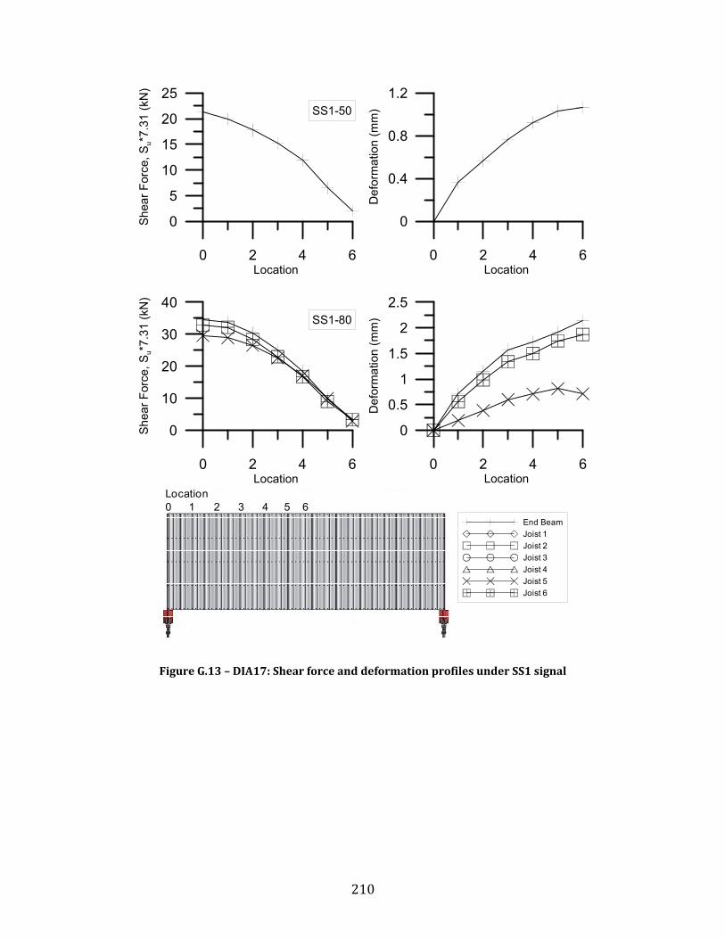
210

Figure G.13 – DIA17: Shear force and deformation profiles under SS1 signal

0 2 4 6Location

0

10

20

30

40

Shea

r For

ce, S

u*7.

31 (k

N)

SS1-80

0 2 4 6Location

0

0.4

0.8

1.2

Def

orm

atio

n (m

m)

0 2 4 6Location

0

0.5

1

1.5

2

2.5

Def

orm

atio

n (m

m)

0 2 4 6Location

0

5

10

15

20

25

Shea

r For

ce, S

u*7.

31 (k

N)

SS1-50

Location0 1 2 3 4 5 6

End BeamJoist 1Joist 2Joist 3Joist 4Joist 5Joist 6

211

Figure G.14 – DIA17: Shear force and deformation profiles under SS3 and SS2 signals

0 2 4 6Location

0

4

8

12

Shea

r For

ce, S

u*7.

31 (k

N)

SS3-50

0 2 4 6Location

0

20

40

60

80

She

ar F

orce

, Su*

7.31

(kN

)

SS3-180

0 2 4 6Location

0

50

100

150

200

250

Shea

r For

ce, S

u*7.

31 (k

N)

SS2-80

0 2 4 6Location

0

0.2

0.4

0.6

0.8

Def

orm

atio

n (m

m)

0 2 4 6Location

0

1

2

3

4

Def

orm

atio

n (m

m)

0 2 4 6Location

0

5

10

15

20

25

Def

orm

atio

n (m

m)

Location0 1 2 3 4 5 6

End BeamJoist 1Joist 2Joist 3Joist 4Joist 5Joist 6

212

Figure G.15 – DIA18: Shear force and deformation profiles under SS1 signal

0 2 4 6Location

0

20

40

60

80

100

Shea

r For

ce, S

u*7.

31 (k

N)

SS1-100

0 2 4 6Location

0

0.4

0.8

1.2

1.6

2

Def

orm

atio

n (m

m)

0 2 4 6Location

0

2

4

6

Def

orm

atio

n (m

m)

0 2 4 6Location

0

10

20

30

Shea

r For

ce, S

u*7.

31 (k

N)

SS1-50

Location0 1 2 3 4 5 6

End BeamJoist 1Joist 2Joist 3Joist 4Joist 5Joist 6

213

Figure G.16 – DIA18: Shear force and deformation profiles under SS3 and SS2 signals

0 2 4 6Location

0

4

8

12

16

Shea

r For

ce, S

u*7.

31 (k

N)

SS3-50

0 2 4 6Location

0

20

40

60

80

Shea

r For

ce, S

u*7.

31 (k

N)

SS3-180

0 2 4 6Location

0

100

200

300

She

ar F

orce

, Su*

7.31

(kN

)

SS2-92

0 2 4 6Location

0

0.2

0.4

0.6

0.8

Def

orm

atio

n (m

m)

0 2 4 6Location

0

1

2

3

4

5

Def

orm

atio

n (m

m)

0 2 4 6Location

0

4

8

12

16

Def

orm

atio

n (m

m)

Location0 1 2 3 4 5 6

End BeamJoist 1Joist 2Joist 3Joist 4Joist 5Joist 6

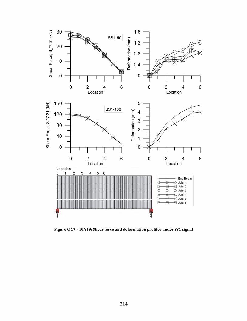
214

Figure G.17 – DIA19: Shear force and deformation profiles under SS1 signal

0 2 4 6Location

0

40

80

120

160

Shea

r For

ce, S

u*7.

31 (k

N)

SS1-100

0 2 4 6Location

0

0.4

0.8

1.2

1.6

Def

orm

atio

n (m

m)

0 2 4 6Location

0

1

2

3

4

5

Def

orm

atio

n (m

m)

0 2 4 6Location

0

10

20

30

Shea

r For

ce, S

u*7.

31 (k

N)

SS1-50

Location0 1 2 3 4 5 6

End BeamJoist 1Joist 2Joist 3Joist 4Joist 5Joist 6

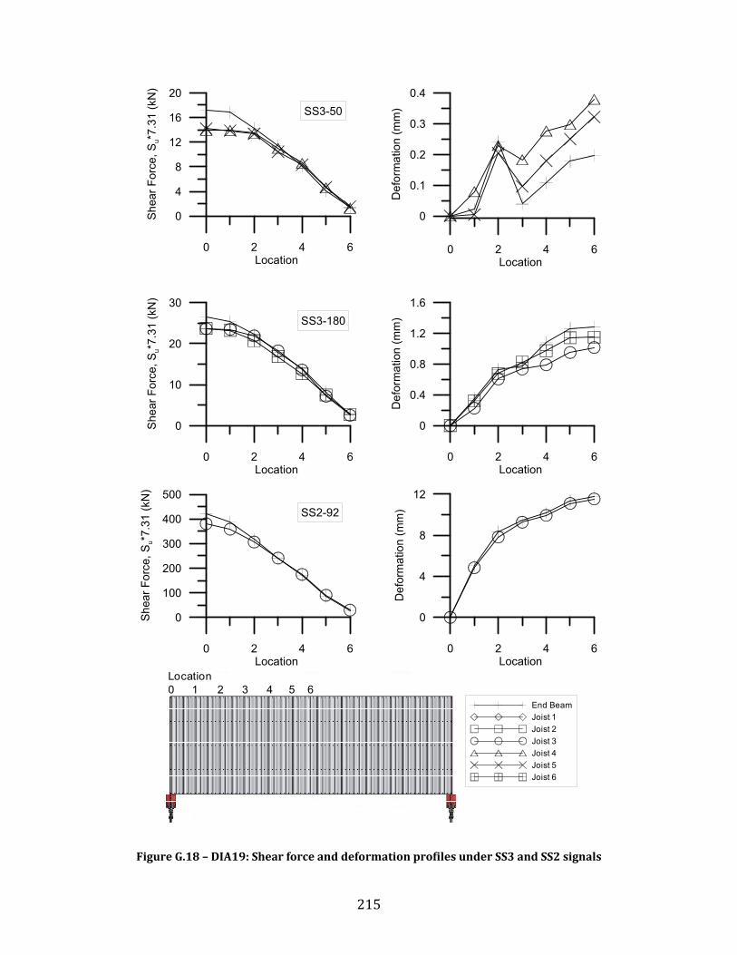
215

Figure G.18 – DIA19: Shear force and deformation profiles under SS3 and SS2 signals

0 2 4 6Location

0

4

8

12

16

20

Shea

r For

ce, S

u*7.

31 (k

N)

SS3-50

0 2 4 6Location

0

10

20

30

She

ar F

orce

, Su*

7.31

(kN

)

SS3-180

0 2 4 6Location

0

100

200

300

400

500

Shea

r For

ce, S

u*7.

31 (k

N)

SS2-92

0 2 4 6Location

0

0.1

0.2

0.3

0.4

Def

orm

atio

n (m

m)

0 2 4 6Location

0

0.4

0.8

1.2

1.6

Def

orm

atio

n (m

m)

0 2 4 6Location

0

4

8

12

Def

orm

atio

n (m

m)

Location0 1 2 3 4 5 6

End BeamJoist 1Joist 2Joist 3Joist 4Joist 5Joist 6

216

Appendix H:

SHEAR FORCE AND DEFORMATION PROFILES FOR

REPAIRED DIAPHRAGM SPECIMENS

217

Figure H.1 – DIA12R: Shear force and deformation profiles under SS1 signal

0 2 4 6Location

0

40

80

120

Shea

r For

ce, S

u*7.

31 (k

N)

SS1-100

0 2 4 6Location

0

0.4

0.8

1.2

1.6

Def

orm

atio

n (m

m)

0 2 4 6Location

0

1

2

3

4

5

Def

orm

atio

n (m

m)

0 2 4 6Location

0

10

20

30

40

Shea

r For

ce, S

u*7.

31 (k

N)

SS1-50

Sheet Overlaps

Location0 1 2 3 4 5 6

End BeamJoist 1Joist 2Joist 3Joist 4Joist 5Joist 6

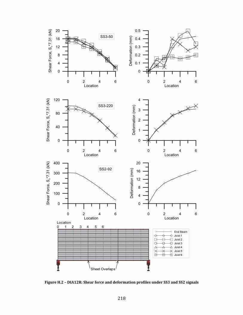
218

Figure H.2 – DIA12R: Shear force and deformation profiles under SS3 and SS2 signals

0 2 4 6Location

0

4

8

12

16

20

Shea

r For

ce, S

u*7.

31 (k

N)

SS3-50

0 2 4 6Location

0

40

80

120

She

ar F

orce

, Su*

7.31

(kN

)

SS3-220

0 2 4 6Location

0

100

200

300

400

Shea

r For

ce, S

u*7.

31 (k

N)

SS2-92

0 2 4 6Location

0

0.1

0.2

0.3

0.4

0.5

Def

orm

atio

n (m

m)

0 2 4 6Location

0

1

2

3

4

Def

orm

atio

n (m

m)

0 2 4 6Location

0

4

8

12

16

20

Def

orm

atio

n (m

m)

Sheet Overlaps

Location0 1 2 3 4 5 6

End BeamJoist 1Joist 2Joist 3Joist 4Joist 5Joist 6

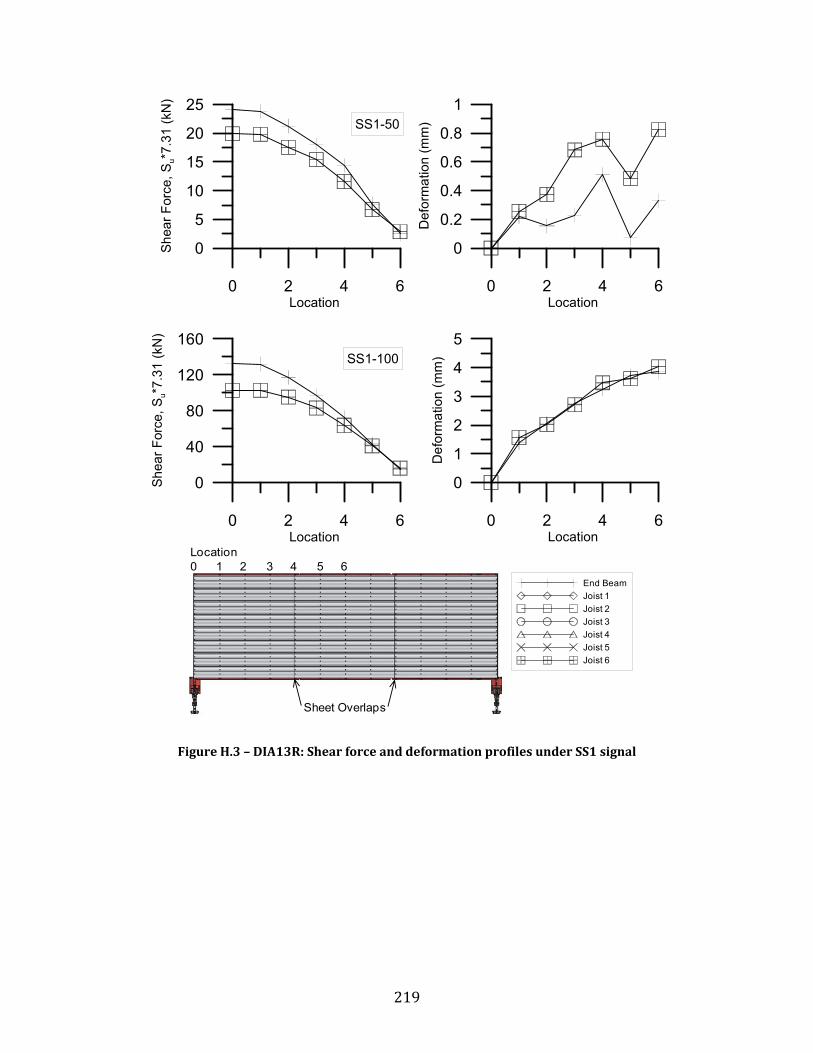
219

Figure H.3 – DIA13R: Shear force and deformation profiles under SS1 signal

0 2 4 6Location

0

40

80

120

160

Shea

r For

ce, S

u*7.

31 (k

N)

SS1-100

0 2 4 6Location

0

0.2

0.4

0.6

0.8

1

Def

orm

atio

n (m

m)

0 2 4 6Location

0

1

2

3

4

5

Def

orm

atio

n (m

m)

0 2 4 6Location

0

5

10

15

20

25

Shea

r For

ce, S

u*7.

31 (k

N)

SS1-50

Sheet Overlaps

Location0 1 2 3 4 5 6

End BeamJoist 1Joist 2Joist 3Joist 4Joist 5Joist 6

220

Figure H.4 – DIA13R: Shear force and deformation profiles under SS3 and SS2 signals

0 2 4 6Location

0

4

8

12

16

Shea

r For

ce, S

u*7.

31 (k

N)

SS3-50

0 2 4 6Location

0

40

80

120

160

She

ar F

orce

, Su*

7.31

(kN

)

SS3-280

0 2 4 6Location

0

100

200

300

400

500

Shea

r For

ce, S

u*7.

31 (k

N)

SS2-92

0 2 4 6Location

0

0.1

0.2

0.3

0.4

Def

orm

atio

n (m

m)

0 2 4 6Location

0

1

2

3

4

5

Def

orm

atio

n (m

m)

0 2 4 6Location

0

10

20

30

40

Def

orm

atio

n (m

m)

Sheet Overlaps

Location0 1 2 3 4 5 6

End BeamJoist 1Joist 2Joist 3Joist 4Joist 5Joist 6

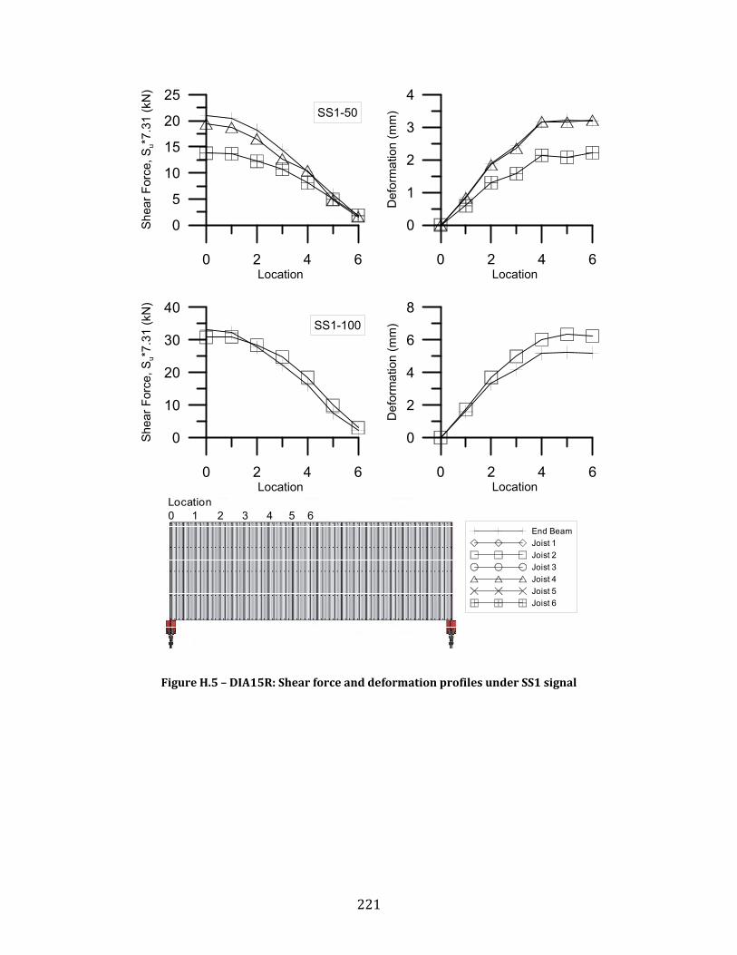
221

Figure H.5 – DIA15R: Shear force and deformation profiles under SS1 signal

0 2 4 6Location

0

10

20

30

40

Shea

r For

ce, S

u*7.

31 (k

N)

SS1-100

0 2 4 6Location

0

1

2

3

4

Def

orm

atio

n (m

m)

0 2 4 6Location

0

2

4

6

8

Def

orm

atio

n (m

m)

0 2 4 6Location

0

5

10

15

20

25

Shea

r For

ce, S

u*7.

31 (k

N)

SS1-50

Location0 1 2 3 4 5 6

End BeamJoist 1Joist 2Joist 3Joist 4Joist 5Joist 6

222

Figure H.6 – DIA15R: Shear force and deformation profiles under SS3 and SS2 signals

0 2 4 6Location

0

2

4

6

8

Shea

r For

ce, S

u*7.

31 (k

N)

SS3-50

0 2 4 6Location

0

10

20

30

40

She

ar F

orce

, Su*

7.31

(kN

)

SS3-240

0 2 4 6Location

0

40

80

120

160

Shea

r For

ce, S

u*7.

31 (k

N)

SS2-80

0 2 4 6Location

0

0.2

0.4

0.6

0.8

1

Def

orm

atio

n (m

m)

0 2 4 6Location

0

2

4

6

8

10

Def

orm

atio

n (m

m)

0 2 4 6Location

0

10

20

30

Def

orm

atio

n (m

m)

Location0 1 2 3 4 5 6

End BeamJoist 1Joist 2Joist 3Joist 4Joist 5Joist 6

223

Figure H.7 – DIA16R: Shear force and deformation profiles under SS1 signal

0 2 4 6Location

0

20

40

60

80

Shea

r For

ce, S

u*7.

31 (k

N)

SS1-140

0 2 4 6Location

0

1

2

3

Def

orm

atio

n (m

m)

0 2 4 6Location

0

2

4

6

Def

orm

atio

n (m

m)

0 2 4 6Location

0

10

20

30

40

Shea

r For

ce, S

u*7.

31 (k

N)

SS1-50

Location0 1 2 3 4 5 6

End BeamJoist 1Joist 2Joist 3Joist 4Joist 5Joist 6

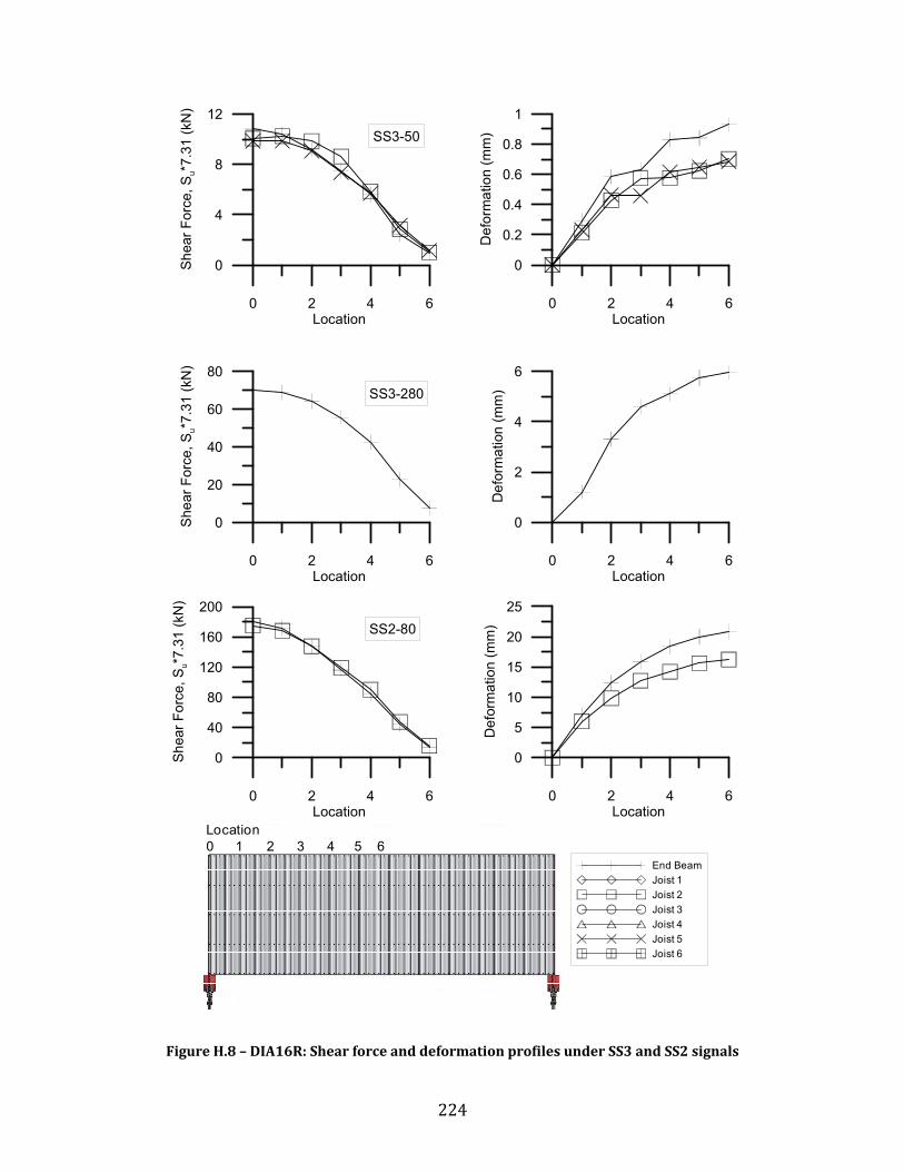
224

Figure H.8 – DIA16R: Shear force and deformation profiles under SS3 and SS2 signals

0 2 4 6Location

0

4

8

12

Shea

r For

ce, S

u*7.

31 (k

N)

SS3-50

0 2 4 6Location

0

20

40

60

80

She

ar F

orce

, Su*

7.31

(kN

)

SS3-280

0 2 4 6Location

0

40

80

120

160

200

Shea

r For

ce, S

u*7.

31 (k

N)

SS2-80

0 2 4 6Location

0

0.2

0.4

0.6

0.8

1

Def

orm

atio

n (m

m)

0 2 4 6Location

0

2

4

6

Def

orm

atio

n (m

m)

0 2 4 6Location

0

5

10

15

20

25

Def

orm

atio

n (m

m)

Location0 1 2 3 4 5 6

End BeamJoist 1Joist 2Joist 3Joist 4Joist 5Joist 6

225

Figure H.9 – DIA17R: Shear force and deformation profiles under SS1 signal

0 2 4 6Location

0

20

40

60

80

100

She

ar F

orce

, Su*

7.31

(kN

)

SS1-120

0 2 4 6Location

0

0.5

1

1.5

2

2.5

Def

orm

atio

n (m

m)

0 2 4 6Location

0

2

4

6

Def

orm

atio

n (m

m)

0 2 4 6Location

0

10

20

30

40

Shea

r For

ce, S

u*7.

31 (k

N)

SS1-50

Location0 1 2 3 4 5 6

End BeamJoist 1Joist 2Joist 3Joist 4Joist 5Joist 6

226

Figure H.10 – DIA17R: Shear force and deformation profiles under SS3 and SS2 signals

0 2 4 6Location

0

4

8

12

Shea

r For

ce, S

u*7.

31 (k

N)

SS3-50

0 2 4 6Location

0

40

80

120

Shea

r For

ce, S

u*7.

31 (k

N)

SS3-260

0 2 4 6Location

0

50

100

150

200

250

She

ar F

orce

, Su*

7.31

(kN

)

SS2-80

0 2 4 6Location

0

0.2

0.4

0.6

Def

orm

atio

n (m

m)

0 2 4 6Location

0

1

2

3

4

5

Def

orm

atio

n (m

m)

0 2 4 6Location

0

4

8

12

Def

orm

atio

n (m

m)

Location0 1 2 3 4 5 6

End BeamJoist 1Joist 2Joist 3Joist 4Joist 5Joist 6

227

Figure H.11 – DIA18R: Shear force and deformation profiles under SS1 signal

0 2 4 6Location

0

20

40

60

80

100

Shea

r For

ce, S

u*7.

31 (k

N)

SS1-120

0 2 4 6Location

0

0.4

0.8

1.2

1.6

2

Def

orm

atio

n (m

m)

0 2 4 6Location

0

1

2

3

4

5

Def

orm

atio

n (m

m)

0 2 4 6Location

0

10

20

30

Shea

r For

ce, S

u*7.

31 (k

N)

SS1-50

Location0 1 2 3 4 5 6

End BeamJoist 1Joist 2Joist 3Joist 4Joist 5Joist 6

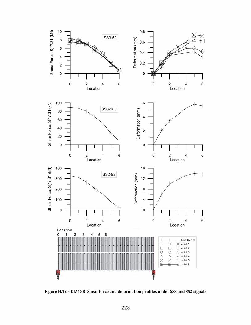
228

Figure H.12 – DIA18R: Shear force and deformation profiles under SS3 and SS2 signals

0 2 4 6Location

0

2

4

6

8

10

Shea

r For

ce, S

u*7.

31 (k

N)

SS3-50

0 2 4 6Location

0

20

40

60

80

100

She

ar F

orce

, Su*

7.31

(kN

)

SS3-280

0 2 4 6Location

0

100

200

300

400

Shea

r For

ce, S

u*7.

31 (k

N)

SS2-92

0 2 4 6Location

0

0.2

0.4

0.6

0.8

Def

orm

atio

n (m

m)

0 2 4 6Location

0

2

4

6

Def

orm

atio

n (m

m)

0 2 4 6Location

0

4

8

12

16

Def

orm

atio

n (m

m)

Location0 1 2 3 4 5 6

End BeamJoist 1Joist 2Joist 3Joist 4Joist 5Joist 6

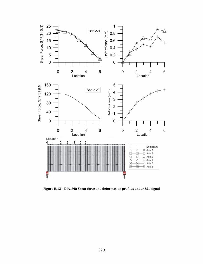
229

Figure H.13 – DIA19R: Shear force and deformation profiles under SS1 signal

0 2 4 6Location

0

40

80

120

160

Shea

r For

ce, S

u*7.

31 (k

N)

SS1-120

0 2 4 6Location

0

0.2

0.4

0.6

0.8

1

Def

orm

atio

n (m

m)

0 2 4 6Location

0

1

2

3

4

5

Def

orm

atio

n (m

m)

0 2 4 6Location

0

5

10

15

20

25

Shea

r For

ce, S

u*7.

31 (k

N)

SS1-50

Location0 1 2 3 4 5 6

End BeamJoist 1Joist 2Joist 3Joist 4Joist 5Joist 6

230

Figure H.14 – DIA19R: Shear force and deformation profiles under SS3 and SS2 signals

0 2 4 6Location

0

4

8

12

16

Shea

r For

ce, S

u*7.

31 (k

N)

SS3-50

0 2 4 6Location

0

40

80

120

She

ar F

orce

, Su*

7.31

(kN

)

SS3-200

0 2 4 6Location

0

100

200

300

400

Shea

r For

ce, S

u*7.

31 (k

N)

SS2-92

0 2 4 6Location

0

0.2

0.4

0.6

0.8

Def

orm

atio

n (m

m)

0 2 4 6Location

0

1

2

3

4

5

Def

orm

atio

n (m

m)

0 2 4 6Location

0

4

8

12

Def

orm

atio

n (m

m)

Location0 1 2 3 4 5 6

End BeamJoist 1Joist 2Joist 3Joist 4Joist 5Joist 6

231

Appendix I:

SHEAR FORCE VS. MID-SPAN DISPLACEMENT HYSTERESES

FOR NEW DIAPHRAGM SPECIMENS

232

Figure I.1 – DIA11: Shear force vs. mid-span displacement for north actuator (left) and south actuator (right)

Figure I.2 – DIA12: Shear force vs. mid-span displacement for north actuator (left) and

south actuator (right)

Figure I.3 – DIA13: Shear force vs. mid-span displacement for north actuator (left) and

south actuator (right)

-0.3 -0.2 -0.1 0 0.1 0.2 0.3δm/L (x102)

-2

-1

0

1

2

S1/S

u

-0.3 -0.2 -0.1 0 0.1 0.2 0.3δm/L (x102)

-2

-1

0

1

2

S2/S

u

-0.2 -0.1 0 0.1 0.2δm/L (x102)

-2

-1

0

1

2

S1/S

u

-0.2 -0.1 0 0.1 0.2δm/L (x102)

-2

-1

0

1

2

S2/S

u

-0.2 -0.1 0 0.1 0.2δm/L (x102)

-2

-1

0

1

2

S1/S

u

-0.2 -0.1 0 0.1 0.2δm/L (x102)

-2

-1

0

1

2

S2/S

u

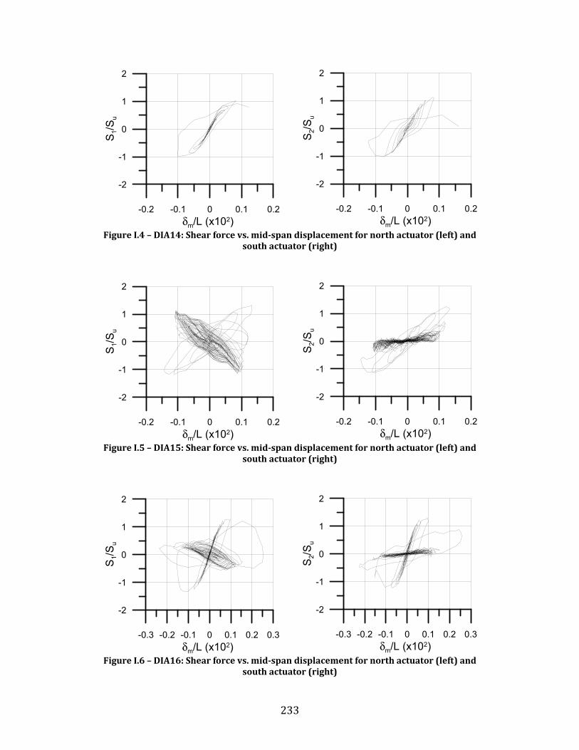
233

Figure I.4 – DIA14: Shear force vs. mid-span displacement for north actuator (left) and south actuator (right)

Figure I.5 – DIA15: Shear force vs. mid-span displacement for north actuator (left) and

south actuator (right)

Figure I.6 – DIA16: Shear force vs. mid-span displacement for north actuator (left) and

south actuator (right)

-0.2 -0.1 0 0.1 0.2δm/L (x102)

-2

-1

0

1

2

S1/S

u

-0.2 -0.1 0 0.1 0.2δm/L (x102)

-2

-1

0

1

2

S2/S

u

-0.2 -0.1 0 0.1 0.2δm/L (x102)

-2

-1

0

1

2

S1/S

u

-0.2 -0.1 0 0.1 0.2δm/L (x102)

-2

-1

0

1

2

S2/S

u

-0.3 -0.2 -0.1 0 0.1 0.2 0.3δm/L (x102)

-2

-1

0

1

2

S1/S

u

-0.3 -0.2 -0.1 0 0.1 0.2 0.3δm/L (x102)

-2

-1

0

1

2

S2/S

u

234

Figure I.7 – DIA17: Shear force vs. mid-span displacement for north actuator (left) and south actuator (right)

Figure I.8 – DIA18: Shear force vs. mid-span displacement for north actuator (left) and

south actuator (right)

Figure I.9 – DIA19: Shear force vs. mid-span displacement for north actuator (left) and

south actuator (right)

-0.3 -0.2 -0.1 0 0.1 0.2 0.3δm/L (x102)

-2

-1

0

1

2

S 1/S

u

-0.3 -0.2 -0.1 0 0.1 0.2 0.3δm/L (x102)

-2

-1

0

1

2

S2/S

u

-0.4 -0.2 0 0.2 0.4δm/L (x102)

-2

-1

0

1

2

S 1/S

u

-0.4 -0.2 0 0.2 0.4δm/L (x102)

-2

-1

0

1

2

S2/S

u

-0.2 -0.1 0 0.1 0.2δm/L (x102)

-2

-1

0

1

2

S 1/S

u

-0.2 -0.1 0 0.1 0.2δm/L (x102)

-2

-1

0

1

2

S2/S

u

235

Appendix J:

SHEAR FORCE VS. MID-SPAN DISPLACEMENT HYSTERESES

FOR REPAIRED DIAPHRAGM SPECIMENS

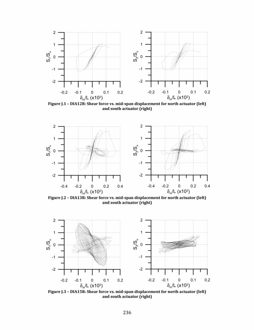
236

Figure J.1 – DIA12R: Shear force vs. mid-span displacement for north actuator (left) and south actuator (right)

Figure J.2 – DIA13R: Shear force vs. mid-span displacement for north actuator (left)

and south actuator (right)

Figure J.3 – DIA15R: Shear force vs. mid-span displacement for north actuator (left)

and south actuator (right)

-0.2 -0.1 0 0.1 0.2δm/L (x102)

-2

-1

0

1

2

S 1/S

u

-0.2 -0.1 0 0.1 0.2δm/L (x102)

-2

-1

0

1

2

S2/S

u

-0.4 -0.2 0 0.2 0.4δm/L (x102)

-2

-1

0

1

2

S 1/S

u

-0.4 -0.2 0 0.2 0.4δm/L (x102)

-2

-1

0

1

2

S2/S

u

-0.2 -0.1 0 0.1 0.2δm/L (x102)

-2

-1

0

1

2

S 1/S

u

-0.2 -0.1 0 0.1 0.2δm/L (x102)

-2

-1

0

1

2

S2/S

u

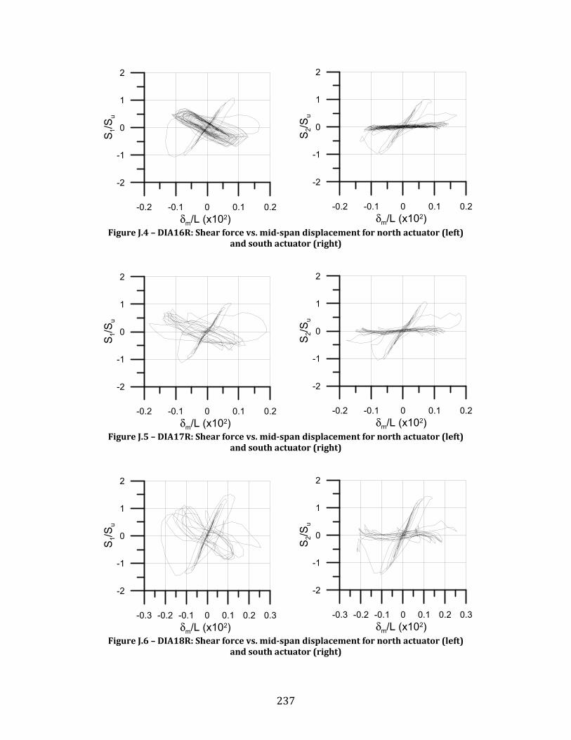
237

Figure J.4 – DIA16R: Shear force vs. mid-span displacement for north actuator (left) and south actuator (right)

Figure J.5 – DIA17R: Shear force vs. mid-span displacement for north actuator (left)

and south actuator (right)

Figure J.6 – DIA18R: Shear force vs. mid-span displacement for north actuator (left)

and south actuator (right)

-0.2 -0.1 0 0.1 0.2δm/L (x102)

-2

-1

0

1

2

S 1/S

u

-0.2 -0.1 0 0.1 0.2δm/L (x102)

-2

-1

0

1

2

S2/S

u

-0.2 -0.1 0 0.1 0.2δm/L (x102)

-2

-1

0

1

2

S 1/S

u

-0.2 -0.1 0 0.1 0.2δm/L (x102)

-2

-1

0

1

2

S2/S

u

-0.3 -0.2 -0.1 0 0.1 0.2 0.3δm/L (x102)

-2

-1

0

1

2

S1/S

u

-0.3 -0.2 -0.1 0 0.1 0.2 0.3δm/L (x102)

-2

-1

0

1

2

S2/S

u

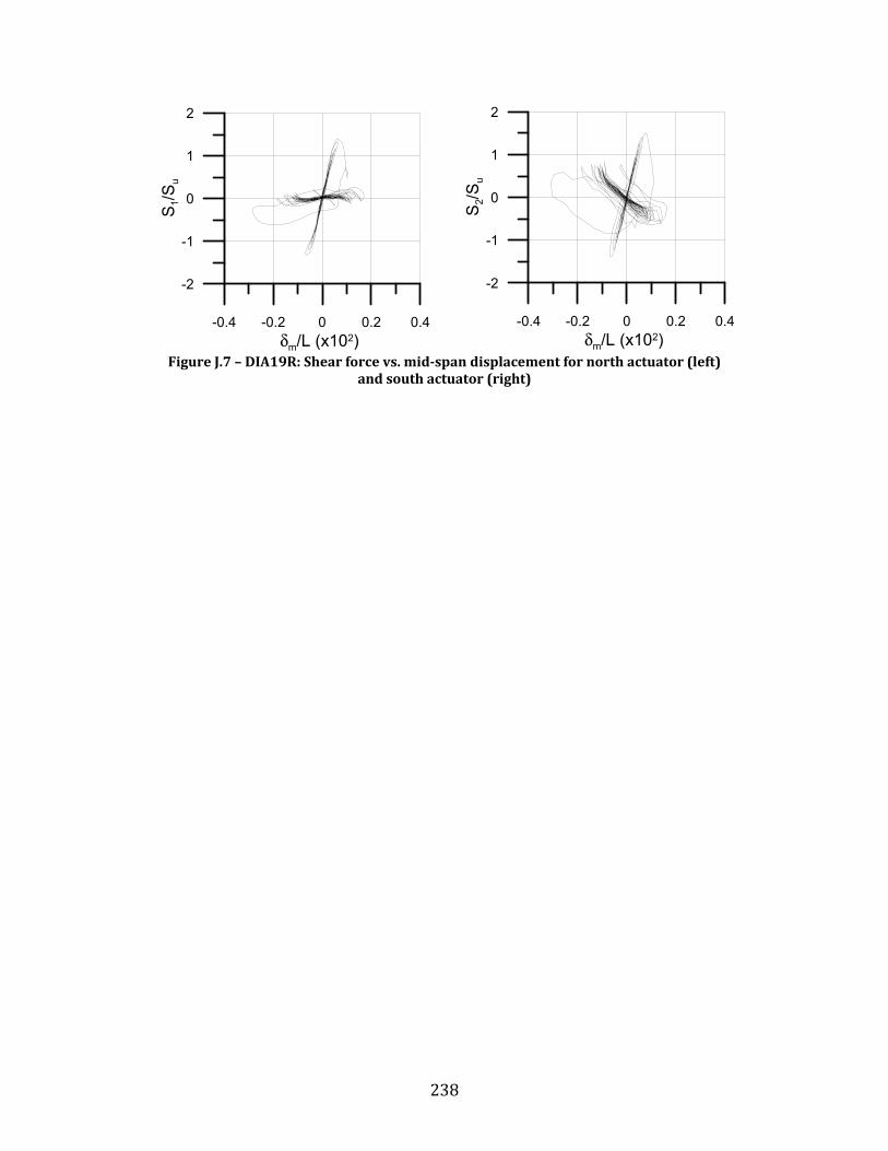
238

Figure J.7 – DIA19R: Shear force vs. mid-span displacement for north actuator (left) and south actuator (right)

-0.4 -0.2 0 0.2 0.4δm/L (x102)

-2

-1

0

1

2

S 1/S

u

-0.4 -0.2 0 0.2 0.4δm/L (x102)

-2

-1

0

1

2

S2/S

u

239

Appendix K:

FASTENER AND MASS OBSERVATION SHEETS

FOR INELASTIC TEST

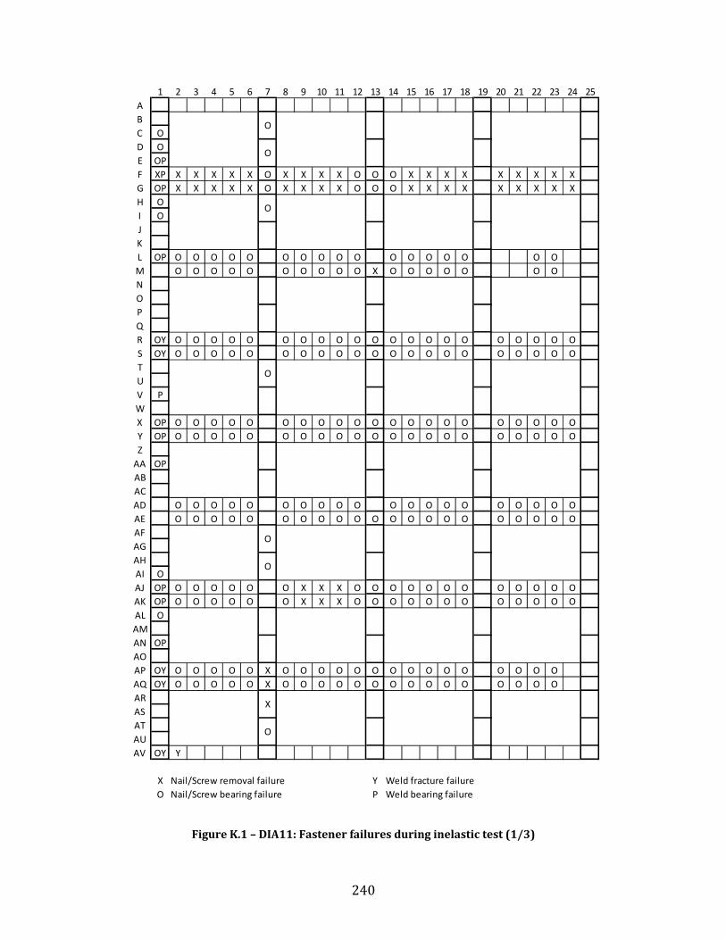
240

Figure K.1 – DIA11: Fastener failures during inelastic test (1/3)

1 2 3 4 5 6 7 8 9 10 11 12 13 14 15 16 17 18 19 20 21 22 23 24 25ABC OD OE OPF XP X X X X X O X X X X O O O X X X X X X X X XG OP X X X X X O X X X X O O O X X X X X X X X XH OI OJKL OP O O O O O O O O O O O O O O O O OM O O O O O O O O O O X O O O O O O ONOPQR OY O O O O O O O O O O O O O O O O O O O O OS OY O O O O O O O O O O O O O O O O O O O O OTUV PWX OP O O O O O O O O O O O O O O O O O O O O OY OP O O O O O O O O O O O O O O O O O O O O OZ

AA OPABACAD O O O O O O O O O O O O O O O O O O O OAE O O O O O O O O O O O O O O O O O O O O OAFAGAHAI OAJ OP O O O O O O X X X O O O O O O O O O O O OAK OP O O O O O O X X X O O O O O O O O O O O OAL OAMAN OPAOAP OY O O O O O X O O O O O O O O O O O O O O OAQ OY O O O O O X O O O O O O O O O O O O O O OARASATAUAV OY Y

X Nail/Screw removal failure Y Weld fracture failureO Nail/Screw bearing failure P Weld bearing failure

O

O

O

O

O

O

X

O

241

Figure K.2 – DIA11: Fastener failures during inelastic test (2/3)

26 27 28 29 30 31 32 33 34 35 36 37 38 39 40 41 42 43 44 45 46 47 48

242

Figure K.3 – DIA11: Fastener failures during inelastic test (3/3)

49 50 51 52 53 54 55 56 57 58 59 60 61 62 63 64 65 66 67 68 69 70 71 72 73

O O O O O O O O O O O O O O O O O OO O O O O O O O O O O O O O O O O O

O O O O O O O O O O X O O O O O O O O OO O O O O O O O O O X O O O O O O O O O

O O O O O O O O O O O O O O O O O O O OX O O O O O O O O O O O O O O O O O O O O

O O O O O O O O O O O O O O O O O O O OO O O O O O O O O O O O O O O O O O O O

O O O O O O O O O O O O O O O O O O O OO O O O O O O O O O O O O O O O O O O O P

O O O O O O O O O O O O O O O O O O O O OPO O O O O O O O O O O O O O O O O O O O OP

O O O O O O O O O O O O O O O O O O O OO O O O O O O O O O O O O O O O O O O O

XY

X

X

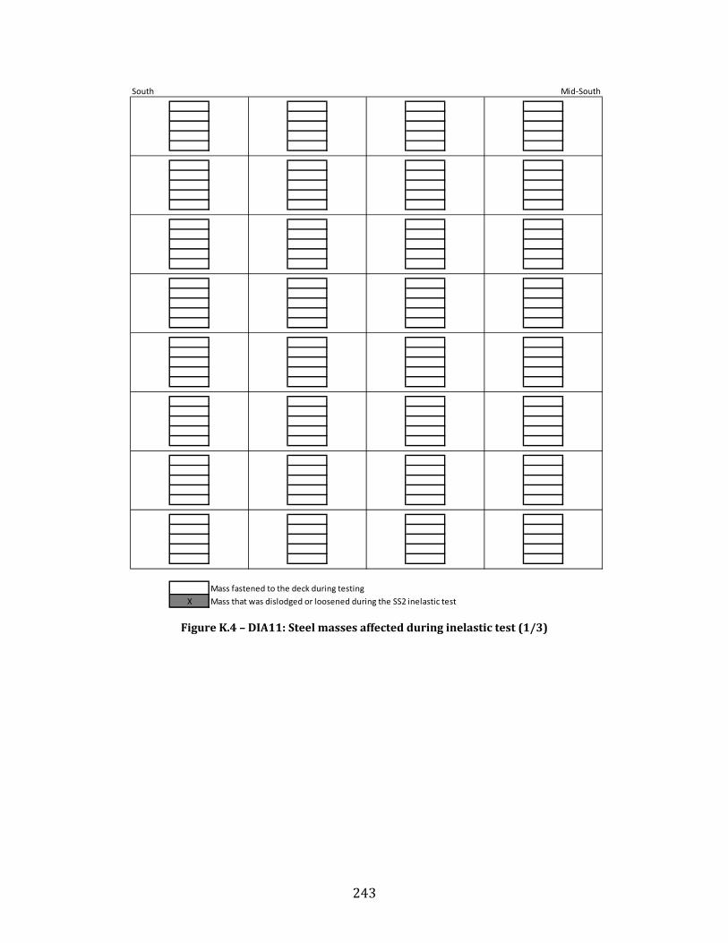
243

Figure K.4 – DIA11: Steel masses affected during inelastic test (1/3)

South

Mass fastened to the deck during testingX Mass that was dislodged or loosened during the SS2 inelastic test

Mid-South

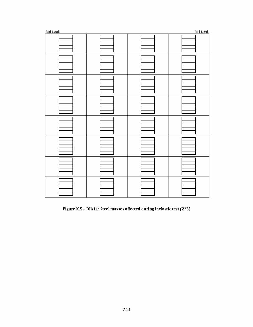
244

Figure K.5 – DIA11: Steel masses affected during inelastic test (2/3)

Mid-South Mid-North

245

Figure K.6 – DIA11: Steel masses affected during inelastic test (3/3)

Mid-North North

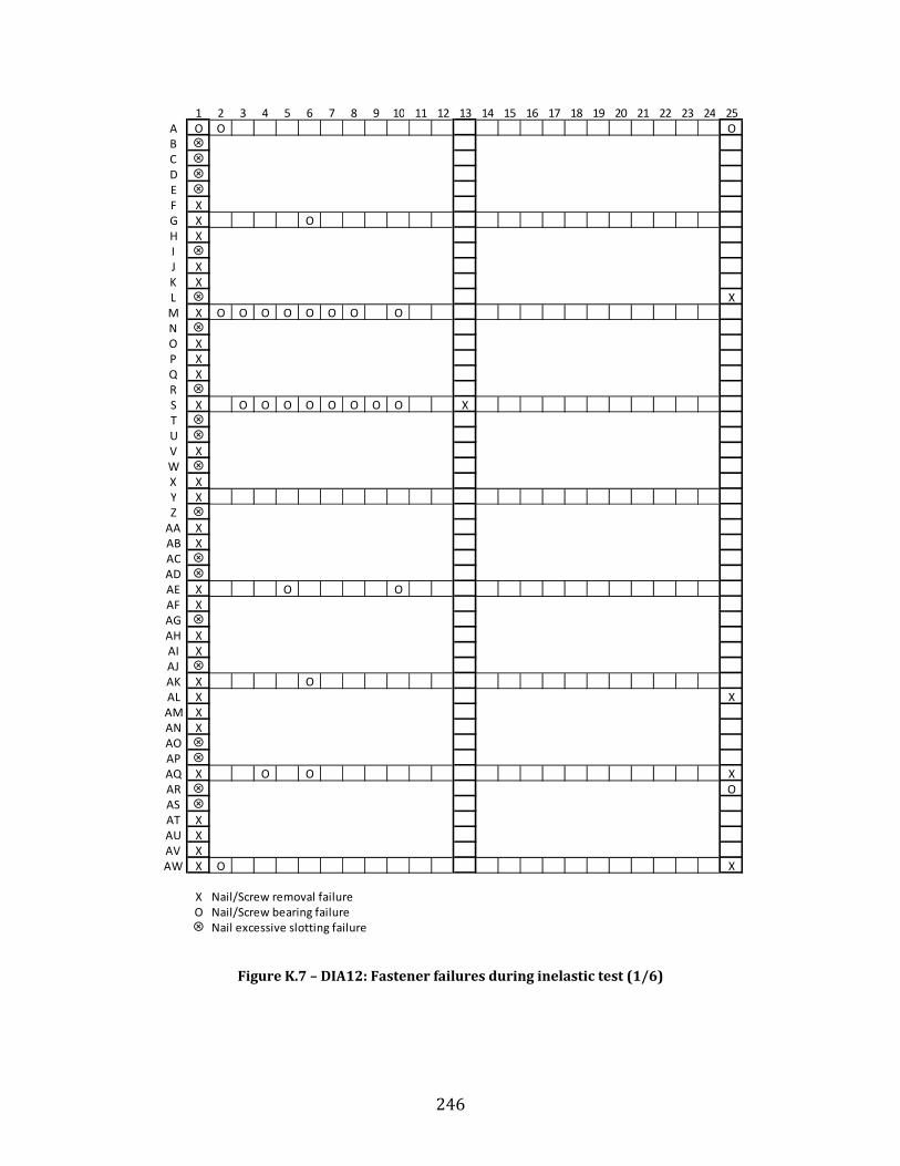
246

Figure K.7 – DIA12: Fastener failures during inelastic test (1/6)

1 2 3 4 5 6 7 8 9 10 11 12 13 14 15 16 17 18 19 20 21 22 23 24 25A O O OBCDEF XG X OH XIJ XK XL XM X O O O O O O O ONO XP XQ XRS X O O O O O O O O XTUV XWX XY XZ

AA XAB XACADAE X O OAF XAGAH XAI XAJAK X OAL X XAM XAN XAOAPAQ X O O XAR OASAT XAU XAV XAW X O X

X Nail/Screw removal failureO Nail/Screw bearing failure

Nail excessive slotting failure

247

Figure K.8 – DIA12: Fastener failures during inelastic test (2/6)

26 27 28 29 30 31 32 33 34 35 36 37 38 39 40 41 42 43 44 45 46 47 48 49O

X

X

X

248

Figure K.9 – DIA12: Fastener failures during inelastic test (3/6)

50 51 52 53 54 55 56 57 58 59 60 61 62 63 64 65 66 67 68 69 70 71 72 73

249

Figure K.10 – DIA12: Fastener failures during inelastic test (4/6)

74 75 76 77 78 79 80 81 82 83 84 85 86 87 88 89 90 91 92 93 94 95 96 97

X

250

Figure K.11 – DIA12: Fastener failures during inelastic test (5/6)

98 99 100 101 102 103 104 105 106 107 108 109 110 111 112 113 114 115 116 117 118 119 120 121

X

XX

X

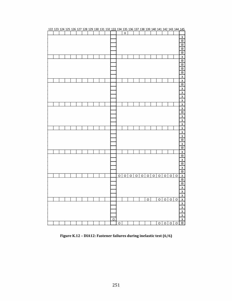
251

Figure K.12 – DIA12: Fastener failures during inelastic test (6/6)

122 123 124 125 126 127 128 129 130 131 132 133 134 135 136 137 138 139 140 141 142 143 144 145X

X

X

XX

XXXXXX

XXXXXX

X

X

X

X

O O O O O O O O O O O X

XXX

O O O O O XXXXX

O XO O O O O

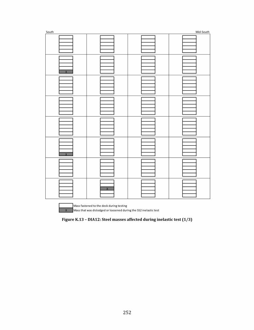
252

Figure K.13 – DIA12: Steel masses affected during inelastic test (1/3)

South

X

X

X

Mass fastened to the deck during testingX Mass that was dislodged or loosened during the SS2 inelastic test

Mid-South

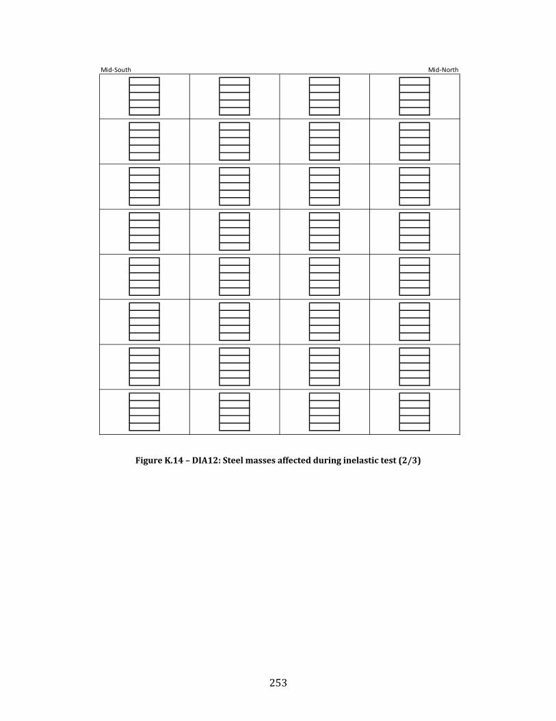
253

Figure K.14 – DIA12: Steel masses affected during inelastic test (2/3)

Mid-South Mid-North

254

Figure K.15 – DIA12: Steel masses affected during inelastic test (3/3)

Mid-North

X

X

X

X

XX

XX

X

North

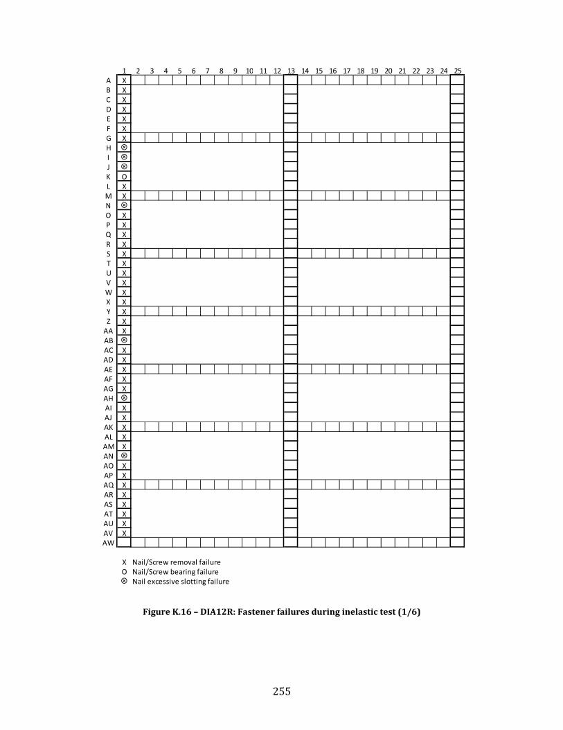
255

Figure K.16 – DIA12R: Fastener failures during inelastic test (1/6)

1 2 3 4 5 6 7 8 9 10 11 12 13 14 15 16 17 18 19 20 21 22 23 24 25A XB XC XD XE XF XG XHIJK OL XM XNO XP XQ XR XS XT XU XV XW XX XY XZ X

AA XABAC XAD XAE XAF XAG XAHAI XAJ XAK XAL XAM XANAO XAP XAQ XAR XAS XAT XAU XAV XAW

X Nail/Screw removal failureO Nail/Screw bearing failure

Nail excessive slotting failure

256

Figure K.17 – DIA12R: Fastener failures during inelastic test (2/6)

26 27 28 29 30 31 32 33 34 35 36 37 38 39 40 41 42 43 44 45 46 47 48 49

X

X

257

Figure K.18 – DIA12R: Fastener failures during inelastic test (3/6)

50 51 52 53 54 55 56 57 58 59 60 61 62 63 64 65 66 67 68 69 70 71 72 73

258

Figure K.19 – DIA12R: Fastener failures during inelastic test (4/6)

74 75 76 77 78 79 80 81 82 83 84 85 86 87 88 89 90 91 92 93 94 95 96 97

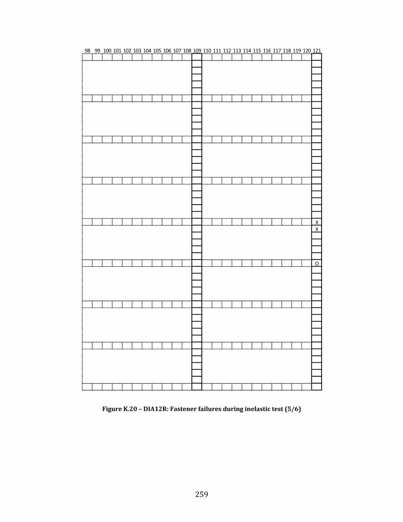
259

Figure K.20 – DIA12R: Fastener failures during inelastic test (5/6)

98 99 100 101 102 103 104 105 106 107 108 109 110 111 112 113 114 115 116 117 118 119 120 121

XX

O

260

Figure K.21 – DIA12R: Fastener failures during inelastic test (6/6)

122 123 124 125 126 127 128 129 130 131 132 133 134 135 136 137 138 139 140 141 142 143 144 145X

O

XXX

O

O

O O O O O

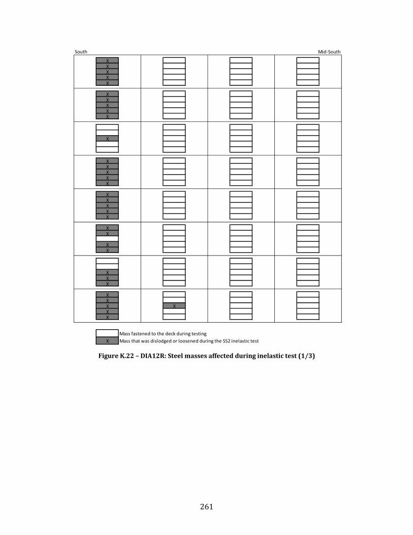
261

Figure K.22 – DIA12R: Steel masses affected during inelastic test (1/3)

South

XXXXX

XXXXX

X

XXXXX

XXXXX

XX

XX

XXX

XXX XXX

Mass fastened to the deck during testingX Mass that was dislodged or loosened during the SS2 inelastic test

Mid-South

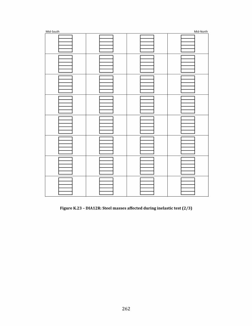
262

Figure K.23 – DIA12R: Steel masses affected during inelastic test (2/3)

Mid-South Mid-North

263

Figure K.24 – DIA12R: Steel masses affected during inelastic test (3/3)

Mid-North

X

North

264

Figure K.25 – DIA13: Fastener failures during inelastic test (1/5)

1 2 3 4 5 6 7 8 9 10 11 12 13 14 15 16 17 18 19 20 21 22 23 24 25ABCDEF XG X O O O O O O O O O O O O O O O O O OHIJKLM X O O O O O O O O O O O O O O O O O O O O O ONOPQR XS X O O O O O O O O O O O O O O OTUVW XX X X XY O O O O O O O O O O O X O O O O O O O O O O O XZ X X

AA XABACAD XAE X O O O O O O O O O O O O O OAF XAG XAH XAI XAJ X XAK X O O O O O O O O O O O O O O O O O O O O O O XAL XAM XAN XAO X XAP XAQ X O O O O O O O O O O O O O O O O O O O O O OARASAT XAUAVAW

X Weld popping/Screw removal failureO Weld/Screw bearing failure

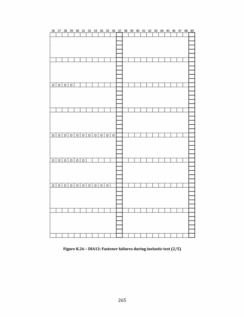
265

Figure K.26 – DIA13: Fastener failures during inelastic test (2/5)

26 27 28 29 30 31 32 33 34 35 36 37 38 39 40 41 42 43 44 45 46 47 48 49

O O O O

O O O O O O O O O O O

O O O O O O

O O O O O O O O O O

266

Figure K.27 – DIA13: Fastener failures during inelastic test (3/5)

50 51 52 53 54 55 56 57 58 59 60 61 62 63 64 65 66 67 68 69 70 71 72 73

267

Figure K.28 – DIA13: Fastener failures during inelastic test (4/5)

74 75 76 77 78 79 80 81 82 83 84 85 86 87 88 89 90 91 92 93 94 95 96 97

268

Figure K.29 – DIA13: Fastener failures during inelastic test (5/5)

98 99 100 101 102 103 104 105 106 107 108 109 110 111 112 113 114 115 116 117 118 119 120 121

O O O O

O O O O

O O O O O O

O O O O O O O O

O O O O O O O O O O O

O O O O O O O O O O O

O O O

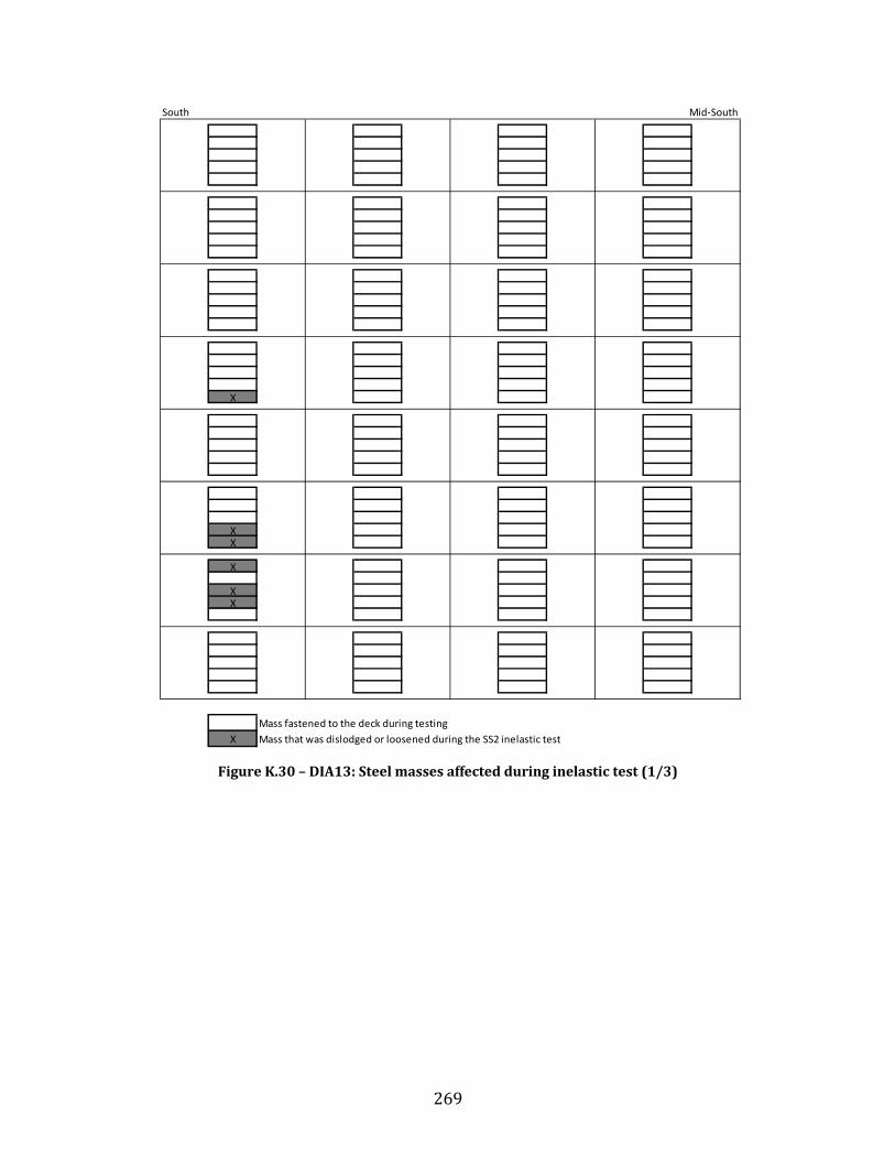
269

Figure K.30 – DIA13: Steel masses affected during inelastic test (1/3)

South

X

XX

X

XX

Mass fastened to the deck during testingX Mass that was dislodged or loosened during the SS2 inelastic test

Mid-South

270

Figure K.31 – DIA13: Steel masses affected during inelastic test (2/3)

Mid-South Mid-North

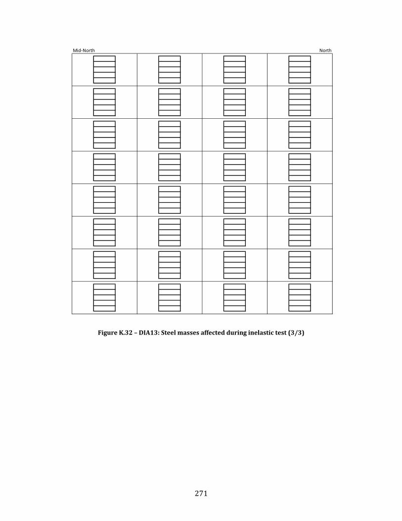
271

Figure K.32 – DIA13: Steel masses affected during inelastic test (3/3)

Mid-North North

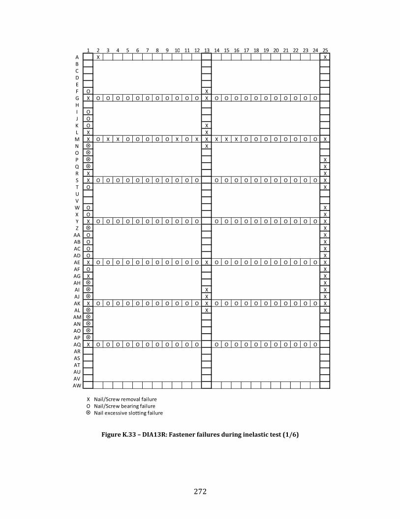
272

Figure K.33 – DIA13R: Fastener failures during inelastic test (1/6)

1 2 3 4 5 6 7 8 9 10 11 12 13 14 15 16 17 18 19 20 21 22 23 24 25A X XBCDEF O XG X O O O O O O O O O O O X O O O O O O O O O O OHI OJ OK O XL X XM X O X X O O O O O X O X X X X X O O O O O O O O XN XOP XQ XR X XS X O O O O O O O O O O O O O O O O O O O O O O XT O XUVW O XX O XY X O O O O O O O O O O O O O O O O O O O O O O XZ X

AA O XAB O XAC O XAD O XAE X O O O O O O O O O O O X O O O O O O O O O O O XAF O XAG X XAH XAI X XAJ X XAK X O O O O O O O O O O O X O O O O O O O O O O O XAL X XAMANAOAPAQ X O O O O O O O O O O O O O O O O O O O O O OARASATAUAVAW

X Nail/Screw removal failureO Nail/Screw bearing failure

Nail excessive slotting failure

273

Figure K.34 – DIA13R: Fastener failures during inelastic test (2/6)

26 27 28 29 30 31 32 33 34 35 36 37 38 39 40 41 42 43 44 45 46 47 48 49X X

XXXXX

O O XX

X XX XX XX X

O O O O O O O O O O O X O O O O O O O O O O O XX X

XXXX

O O O XX X

XXX

X XO O O O O O O O O O O O O O O O O O O O O O X

XXXXX

O O O O O O O O X XXXXX

X XO O O O O O O O O O O X O O O O O O O O O O O X

X XXXXX

O O O O O O O O O O X O O O O O O O O O O O XXXXXXX

274

Figure K.35 – DIA13R: Fastener failures during inelastic test (3/6)

50 51 52 53 54 55 56 57 58 59 60 61 62 63 64 65 66 67 68 69 70 71 72 73X

O O

O

O

O

X X X X X

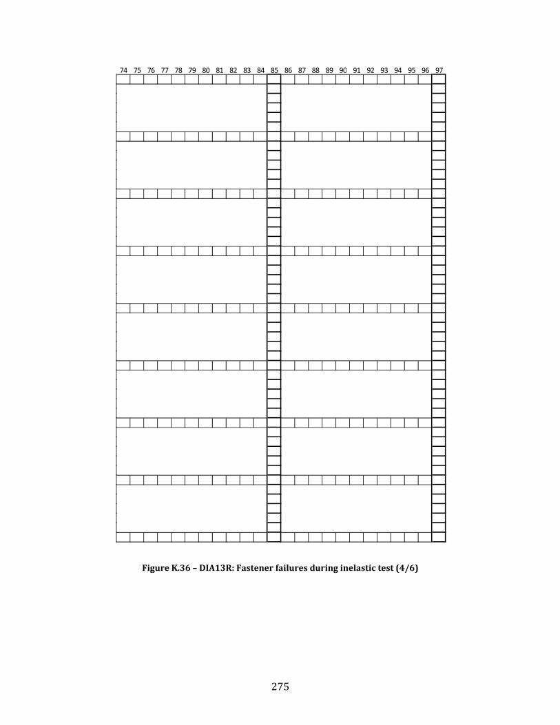
275

Figure K.36 – DIA13R: Fastener failures during inelastic test (4/6)

74 75 76 77 78 79 80 81 82 83 84 85 86 87 88 89 90 91 92 93 94 95 96 97

276

Figure K.37 – DIA13R: Fastener failures during inelastic test (5/6)

98 99 100 101 102 103 104 105 106 107 108 109 110 111 112 113 114 115 116 117 118 119 120 121

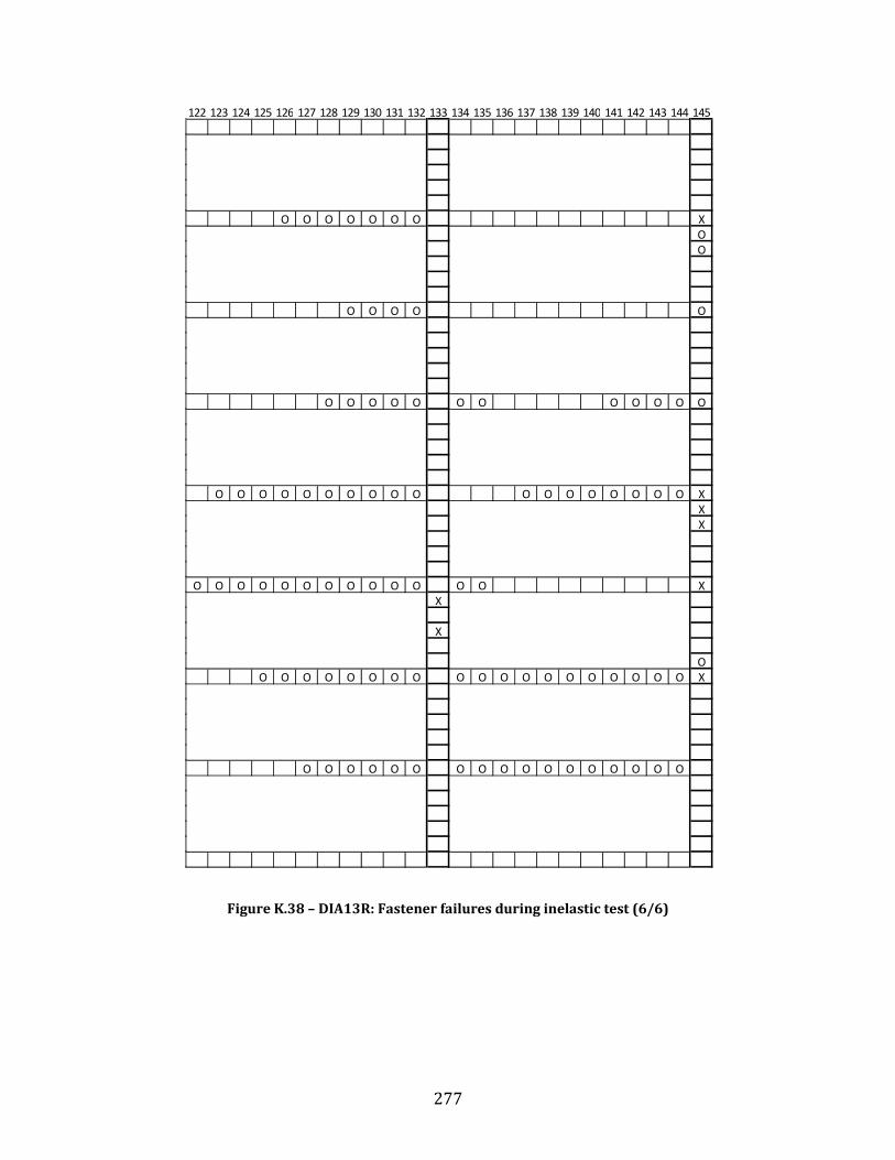
277

Figure K.38 – DIA13R: Fastener failures during inelastic test (6/6)

122 123 124 125 126 127 128 129 130 131 132 133 134 135 136 137 138 139 140 141 142 143 144 145

O O O O O O O XOO

O O O O O

O O O O O O O O O O O O

O O O O O O O O O O O O O O O O O O XXX

O O O O O O O O O O O O O XX

X

OO O O O O O O O O O O O O O O O O O O X

O O O O O O O O O O O O O O O O O

278

Figure K.39 – DIA13R: Steel masses affected during inelastic test (1/3)

South

XX

XX X

X

X

Mass fastened to the deck during testingX Mass that was dislodged or loosened during the SS2 inelastic test

Mid-South

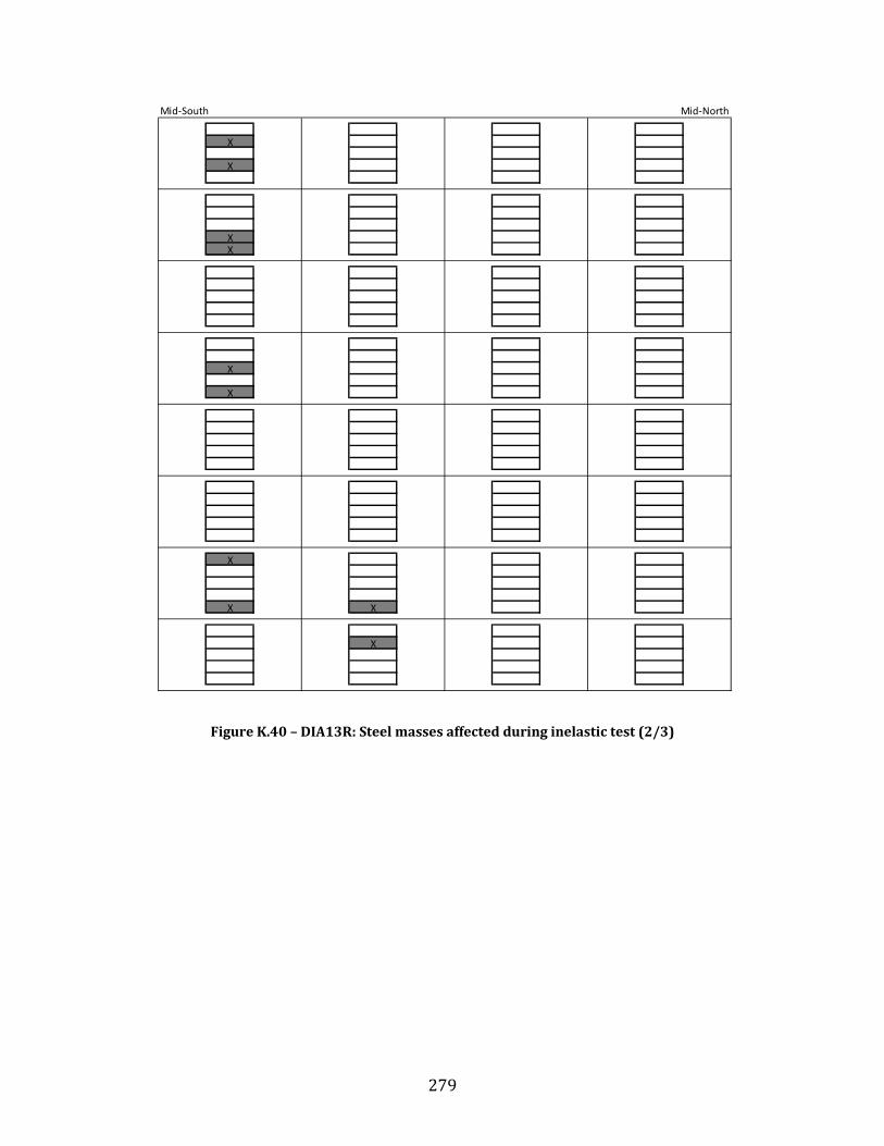
279

Figure K.40 – DIA13R: Steel masses affected during inelastic test (2/3)

Mid-South

X

X

XX

X

X

X

X X

X

Mid-North

280

Figure K.41 – DIA13R: Steel masses affected during inelastic test (3/3)

Mid-North North

281

Figure K.42 – DIA14: Fastener failures during inelastic test (1/6)

1 2 3 4 5 6 7 8 9 10 11 12 13 14 15 16 17 18 19 20 21 22 23 24 25 26 27 28 29 30 31 32 33 34 35

X

X

XXXX

XXXXXXXOOO

XX

XXXXXXX

XXXX

XXXXXXXXXXXXX

X Nail/Screw removal failureO Nail/Screw bearing failure

Nail excessive slotting failure

282

Figure K.43 – DIA14: Fastener failures during inelastic test (2/6)

36 37 38 39 40 41 42 43 44 45 46 47 48 49 50 51 52 53 54 55 56 57 58 59 60 61 62 63 64 65 66 67 68 69

X

X

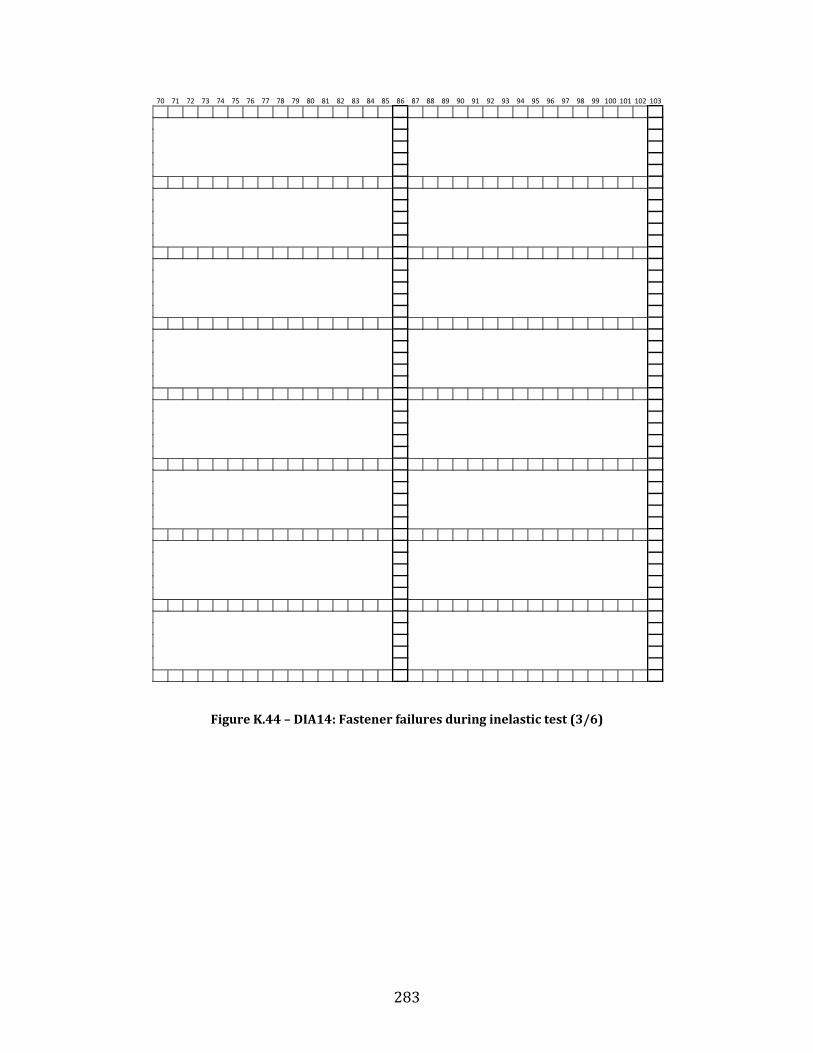
283

Figure K.44 – DIA14: Fastener failures during inelastic test (3/6)

70 71 72 73 74 75 76 77 78 79 80 81 82 83 84 85 86 87 88 89 90 91 92 93 94 95 96 97 98 99 100 101 102 103

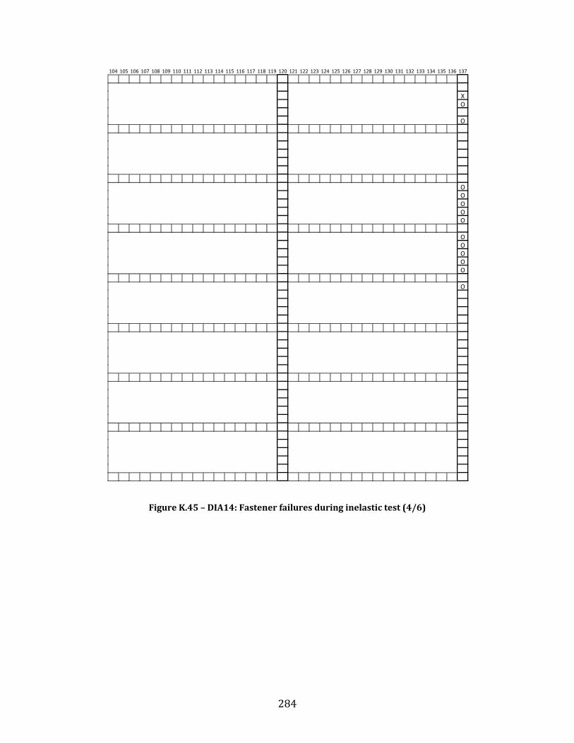
284

Figure K.45 – DIA14: Fastener failures during inelastic test (4/6)

104 105 106 107 108 109 110 111 112 113 114 115 116 117 118 119 120 121 122 123 124 125 126 127 128 129 130 131 132 133 134 135 136 137

XO

O

OOOOO

OOOOO

O

285

Figure K.46 – DIA14: Fastener failures during inelastic test (5/6)

138 139 140 141 142 143 144 145 146 147 148 149 150 151 152 153 154 155 156 157 158 159 160 161 162 163 164 165 166 167 168 169 170 171

X

X

X

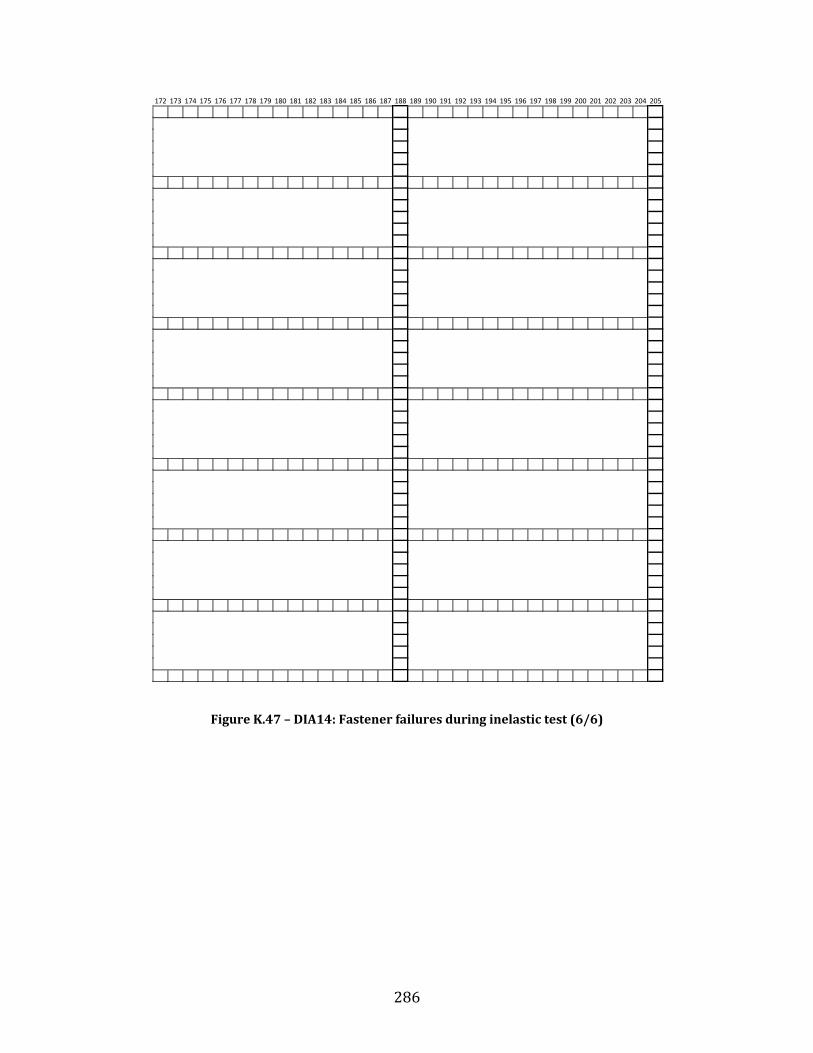
286

Figure K.47 – DIA14: Fastener failures during inelastic test (6/6)

172 173 174 175 176 177 178 179 180 181 182 183 184 185 186 187 188 189 190 191 192 193 194 195 196 197 198 199 200 201 202 203 204 205

287

Figure K.48 – DIA14: Steel masses affected during inelastic test (1/3)

South

Mass fastened to the deck during testingX Mass that was dislodged or loosened during the SS2 inelastic test

Mid-South

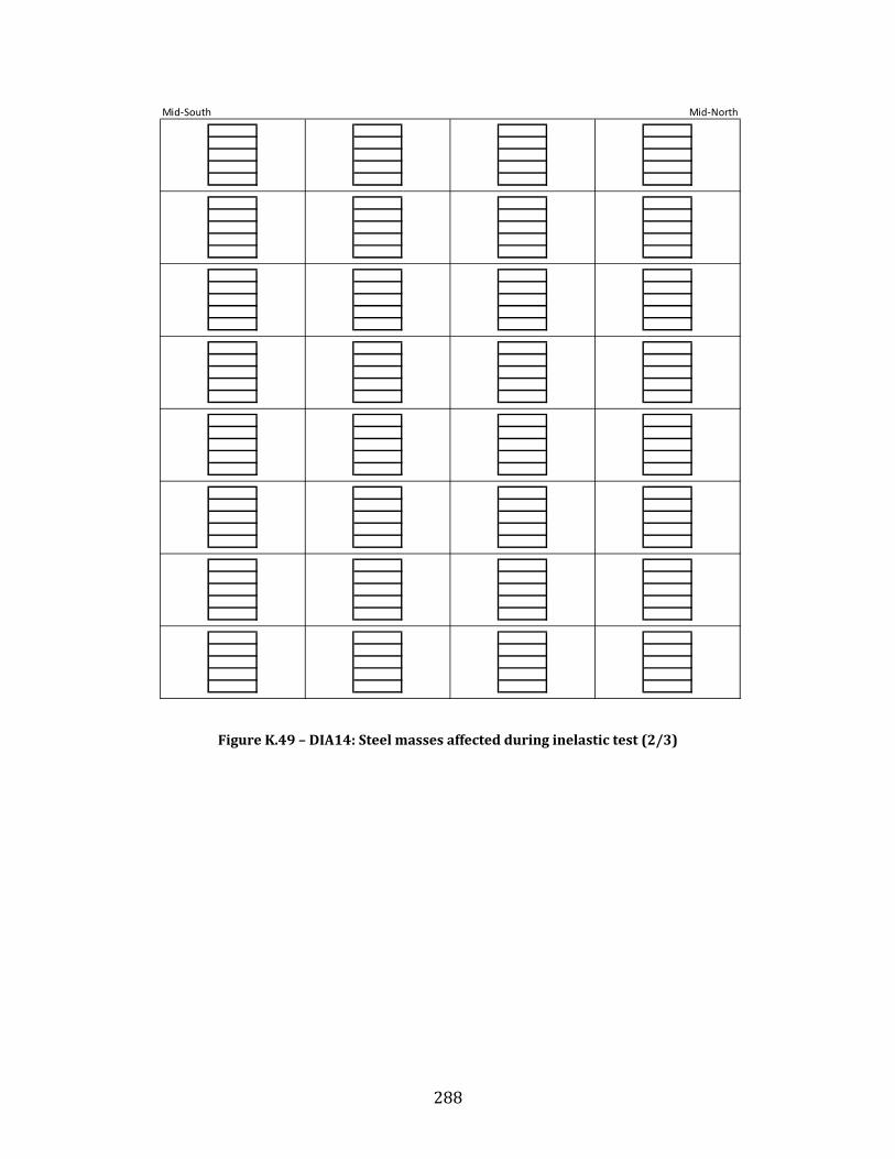
288

Figure K.49 – DIA14: Steel masses affected during inelastic test (2/3)

Mid-South Mid-North

289

Figure K.50 – DIA14: Steel masses affected during inelastic test (3/3)

Mid-North North

290

Figure K.51 – DIA15: Fastener failures during inelastic test (1/5)

1 2 3 5 6 8 9 11 12 14 15A X X X X X X X X X XBCDEFG X X X X X XHIJKLM X X X X X X X XNOPQRS X X X X X X X X X XTUVQXY O X X X X X X X X X X X

X Weld popping/Button-punch removal failureO Weld/Button-punch bearing failure

XXXX

X

XX

XXXXX

X

X

XX

X

XXX

131074 16

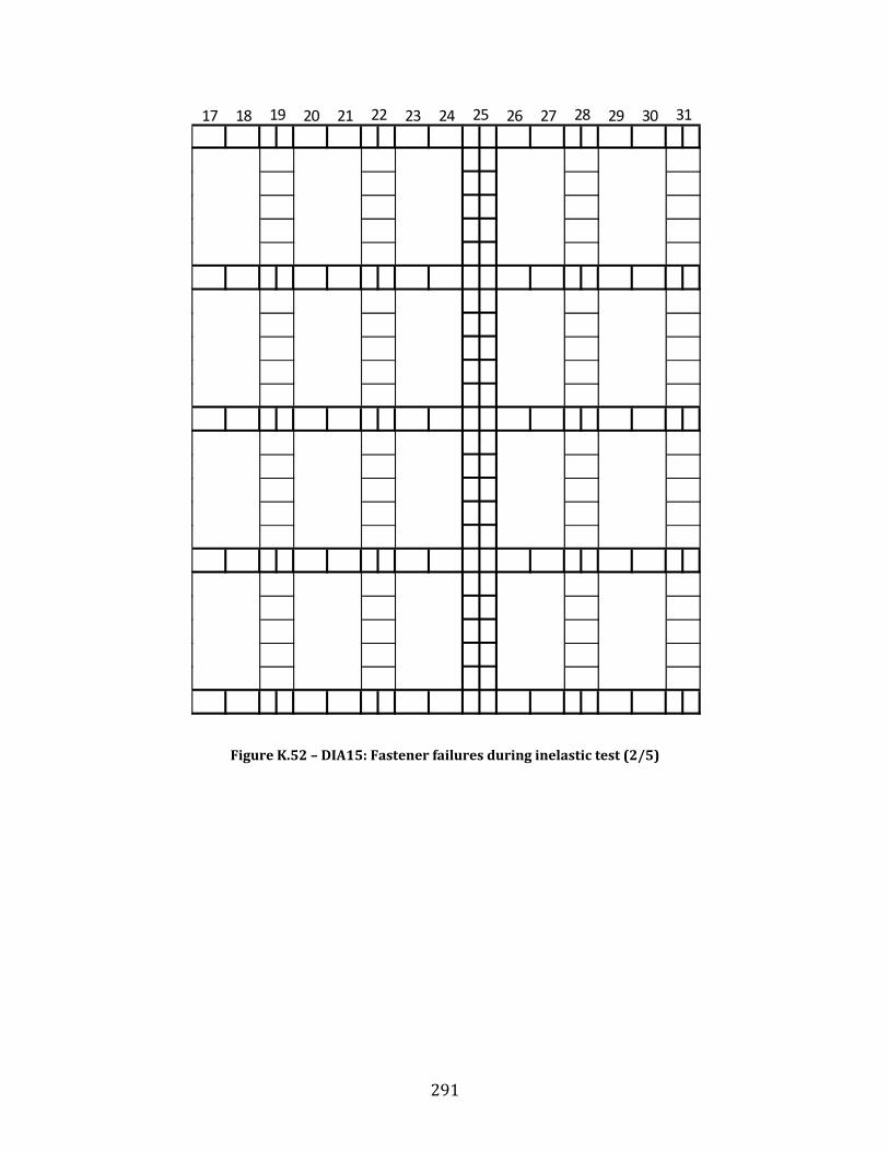
291

Figure K.52 – DIA15: Fastener failures during inelastic test (2/5)

17 18 20 21 23 24 26 27 29 30 3128252219

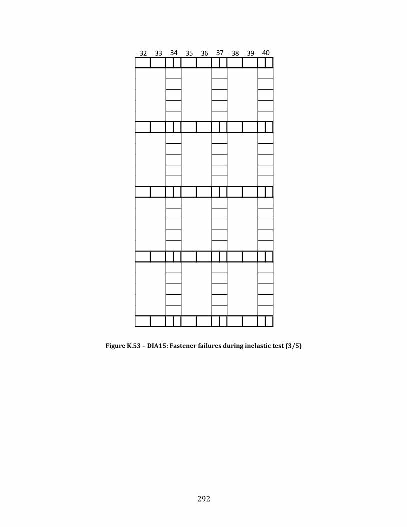
292

Figure K.53 – DIA15: Fastener failures during inelastic test (3/5)

32 33 35 36 38 39 403734

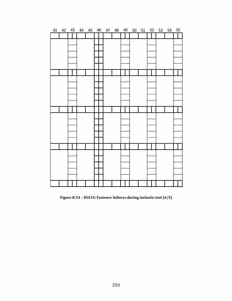
293

Figure K.54 – DIA15: Fastener failures during inelastic test (4/5)

41 42 44 45 47 48 50 51 53 54 555243 4946

294

Figure K.55 – DIA15: Fastener failures during inelastic test (5/5)

56 57 59 60 62 63 65 66 68 69 70

X X

X

67646158

295

Figure K.56 – DIA15: Steel masses affected during inelastic test (1/3)

South Mid-South

Mass fastened to the deck during testingMass that was dislodged or loosened during the SS2 inelastic testX

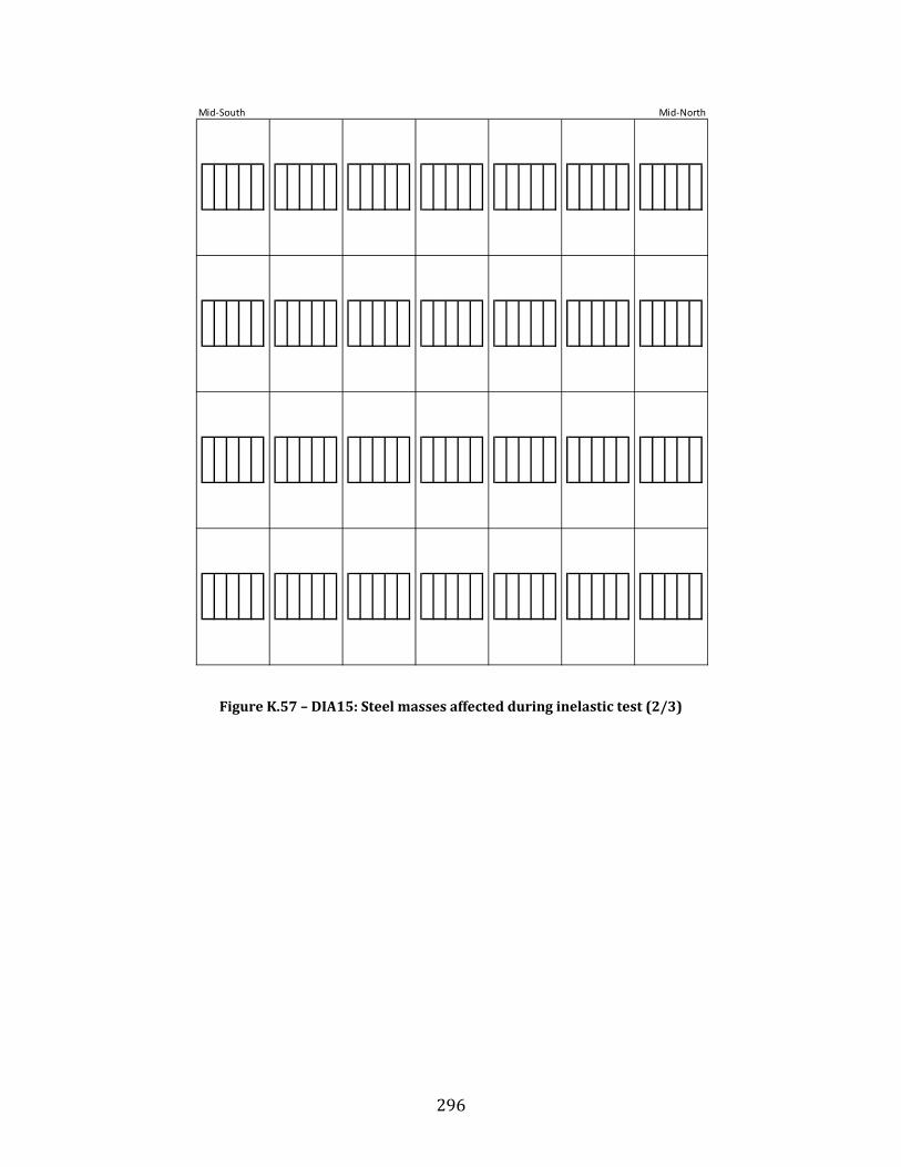
296

Figure K.57 – DIA15: Steel masses affected during inelastic test (2/3)

Mid-South Mid-North

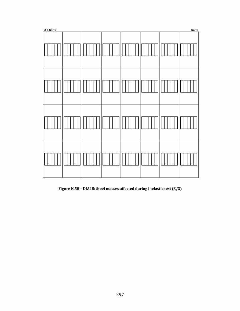
297

Figure K.58 – DIA15: Steel masses affected during inelastic test (3/3)

Mid-North North

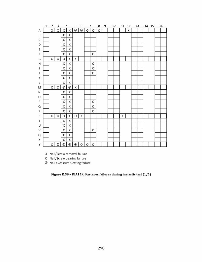
298

Figure K.59 – DIA15R: Fastener failures during inelastic test (1/5)

1 2 3 5 6 8 9 11 12 14 15A X X X X O O O XB X XC X XD X XE X XF X X OG O O O X XH X X OI X X OJ X X OK X XL X XM O O XN X XO X XP X X OQ X X OR X X OS O O O X O X XT X XU X XV X X OQ X XX X XY O O O O

X Nail/Screw removal failureO Nail/Screw bearing failure

Nail excessive slotting failure

4 7 10 13 16

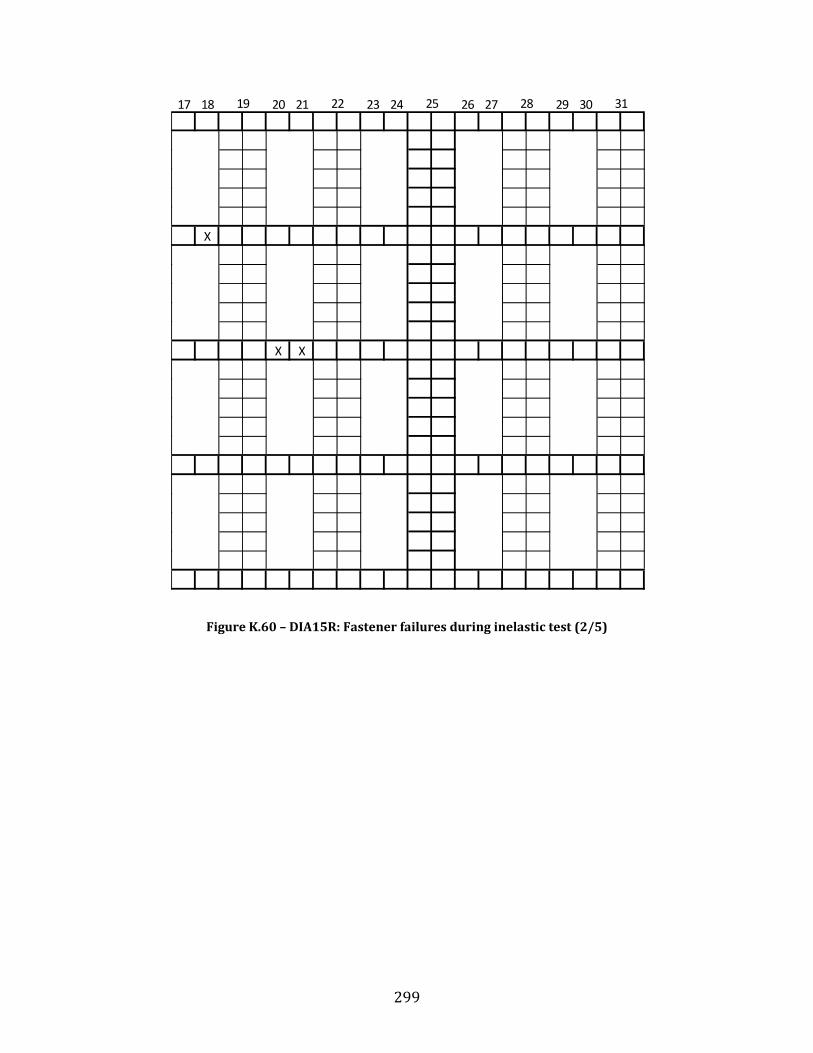
299

Figure K.60 – DIA15R: Fastener failures during inelastic test (2/5)

17 18 20 21 23 24 26 27 29 30

X

X X

19 22 28 3125

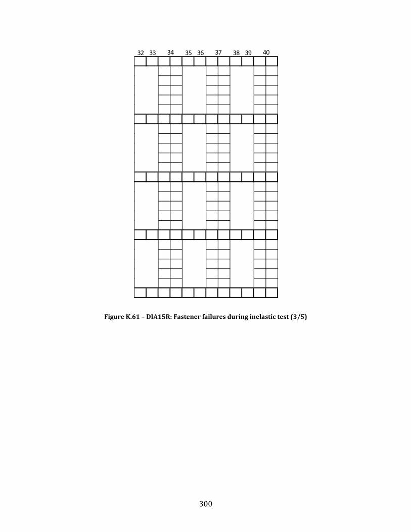
300

Figure K.61 – DIA15R: Fastener failures during inelastic test (3/5)

32 33 35 36 38 39 403734

301

Figure K.62 – DIA15R: Fastener failures during inelastic test (4/5)

41 42 44 45 47 48 50 51 53 544643 49 52 55

302

Figure K.63 – DIA15R: Fastener failures during inelastic test (5/5)

56 57 59 60 62 63 65 66 68 69 70

O OO O

O

6758 61 64

303

Figure K.64 – DIA15R: Steel masses affected during inelastic test (1/3)

South Mid-South

Mass fastened to the deck during testingMass that was dislodged or loosened during the SS2 inelastic testX

304

Figure K.65 – DIA15R: Steel masses affected during inelastic test (2/3)

Mid-South Mid-North

305

Figure K.66 – DIA15R: Steel masses affected during inelastic test (3/3)

Mid-North North

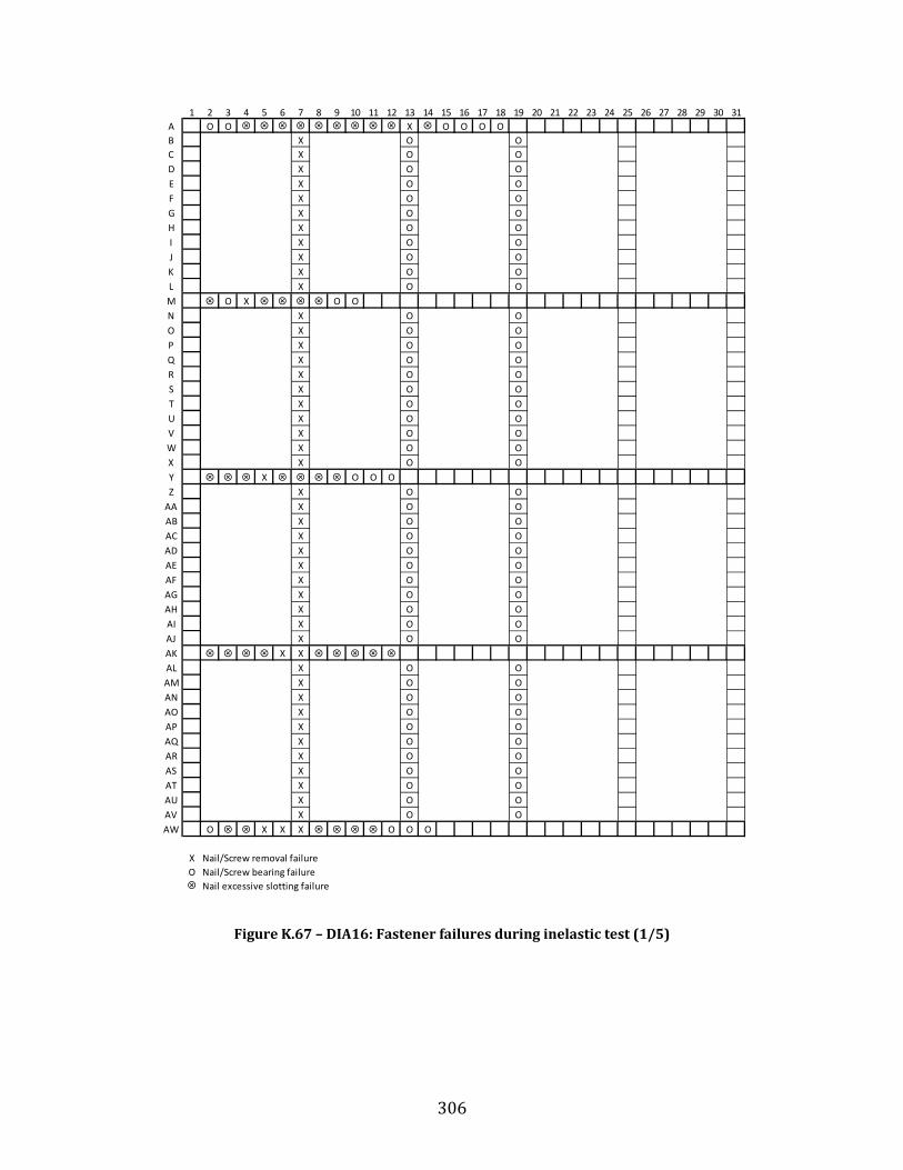
306

Figure K.67 – DIA16: Fastener failures during inelastic test (1/5)

1 2 3 4 5 6 7 8 9 10 11 12 13 14 15 16 17 18 19 20 21 22 23 24 25 26 27 28 29 30 31A O O X O O O OB X O OC X O OD X O OE X O OF X O OG X O OH X O OI X O OJ X O OK X O OL X O OM O X O ON X O OO X O OP X O OQ X O OR X O OS X O OT X O OU X O OV X O OW X O OX X O OY X O O OZ X O O

AA X O OAB X O OAC X O OAD X O OAE X O OAF X O OAG X O OAH X O OAI X O OAJ X O OAK X XAL X O OAM X O OAN X O OAO X O OAP X O OAQ X O OAR X O OAS X O OAT X O OAU X O OAV X O OAW O X X X O O O

X Nail/Screw removal failureO Nail/Screw bearing failure

Nail excessive slotting failure

307

Figure K.68 – DIA16: Fastener failures during inelastic test (2/5)

32 33 34 35 36 37 38 39 40 41 42 43 44 45 46 47 48 49 50 51 52 53 54 55 56 57 58 59 60 61

308

Figure K.69 – DIA16: Fastener failures during inelastic test (3/5)

62 63 64 65 66 67 68 69 70 71 72 73 74 75 76 77 78 79

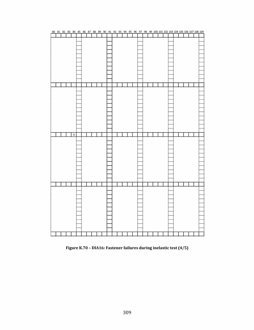
309

Figure K.70 – DIA16: Fastener failures during inelastic test (4/5)

80 81 82 83 84 85 86 87 88 89 90 91 92 93 94 95 96 97 98 99 100 101 102 103 104 105 106 107 108 109

X

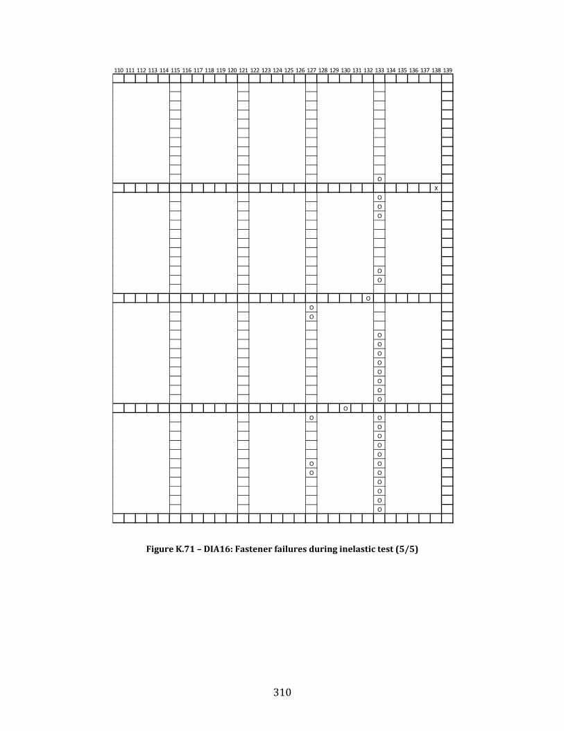
310

Figure K.71 – DIA16: Fastener failures during inelastic test (5/5)

110 111 112 113 114 115 116 117 118 119 120 121 122 123 124 125 126 127 128 129 130 131 132 133 134 135 136 137 138 139

OX

OOO

OO

OOO

OOOOOOOO

OO O

OOOO

O OO O

OOOO

311

Figure K.72 – DIA16: Steel masses affected during inelastic test (1/3)

South Mid-South

Mass fastened to the deck during testingMass that was dislodged or loosened during the SS2 inelastic testX

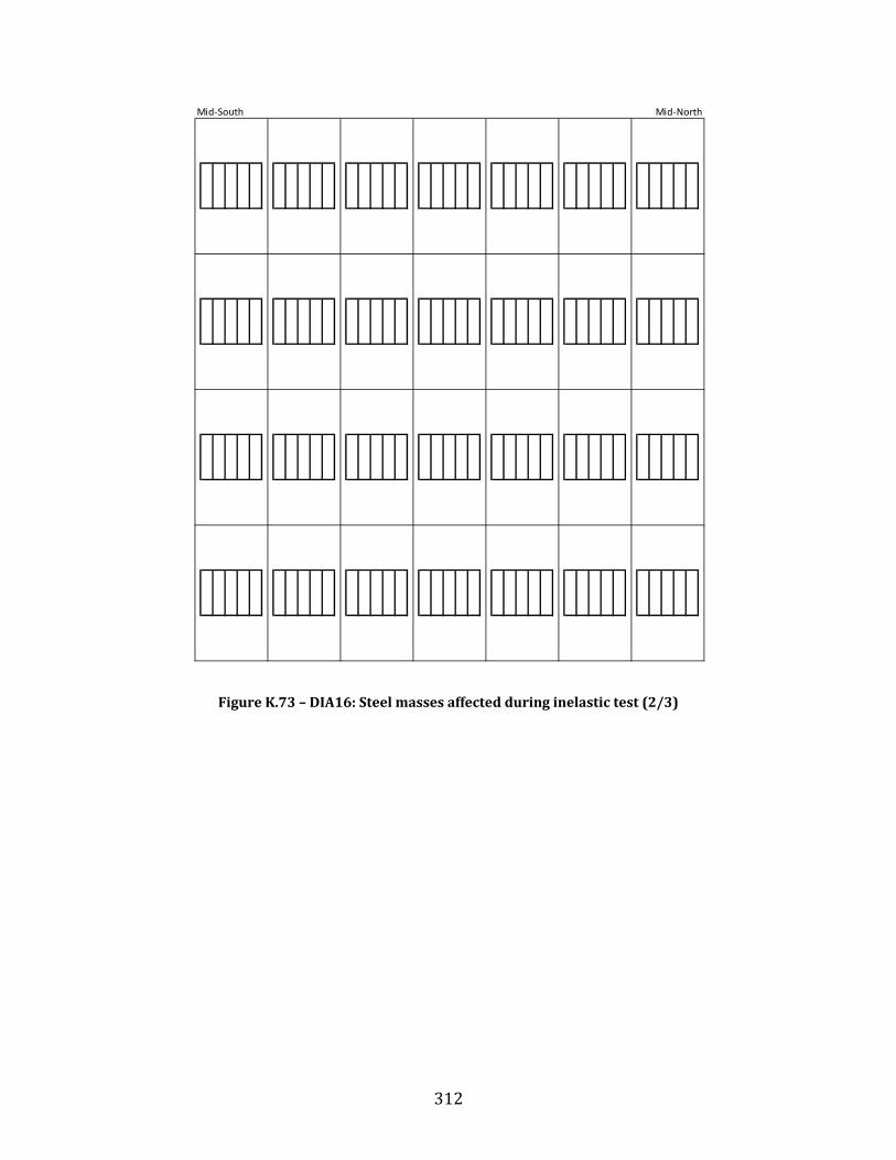
312

Figure K.73 – DIA16: Steel masses affected during inelastic test (2/3)

Mid-South Mid-North

313

Figure K.74 – DIA16: Steel masses affected during inelastic test (3/3)

Mid-North North

X

314

Figure K.75 – DIA16R: Fastener failures during inelastic test (1/5)

1 2 3 4 5 6 7 8 9 10 11 12 13 14 15 16 17 18 19 20 21 22 23 24 25 26 27 28 29 30 31XX

B XC XD XE XF XG XH XI XJ XK XL X

N XO XP XQ XR XS XT XU XV XW XX X

Z XAA XAB XAC XAD XAE XAF XAG XAH XAI XAJ X

XX

AL XX

AN XAO XAP XAQ XAR XAS XAT XAU XAV X

XX

X Nail/Screw removal failureO Nail/Screw bearing failure

Nail excessive slotting failure

O

O X X X

O O O X

X O O

AW

A

M

Y

AK

315

Figure K.76 – DIA16R: Fastener failures during inelastic test (2/5)

32 33 34 35 36 37 38 39 40 41 42 43 44 45 46 47 48 49 50 51 52 53 54 55 56 57 58 59 60 61

316

Figure K.77 – DIA16R: Fastener failures during inelastic test (3/5)

62 63 64 65 66 67 68 69 70 71 72 73 74 75 76 77 78 79

317

Figure K.78 – DIA16R: Fastener failures during inelastic test (4/5)

80 81 82 83 84 85 86 87 88 89 90 91 92 93 94 95 96 97 98 99 100 101 102 103 104 105 106 107 108 109

318

Figure K.79 – DIA16R: Fastener failures during inelastic test (5/5)

110 111 112 113 114 115 116 117 118 119 120 121 122 123 124 125 126 127 128 129 130 131 132 133 134 135 136 137 138 139

O

O

OO

O OOO

OO

O

O OO

O

O

OO

319

Figure K.80 – DIA16R: Steel masses affected during inelastic test (1/3)

South Mid-South

Mass fastened to the deck during testingMass that was dislodged or loosened during the SS2 inelastic testX

320

Figure K.81 – DIA16R: Steel masses affected during inelastic test (2/3)

Mid-South Mid-North

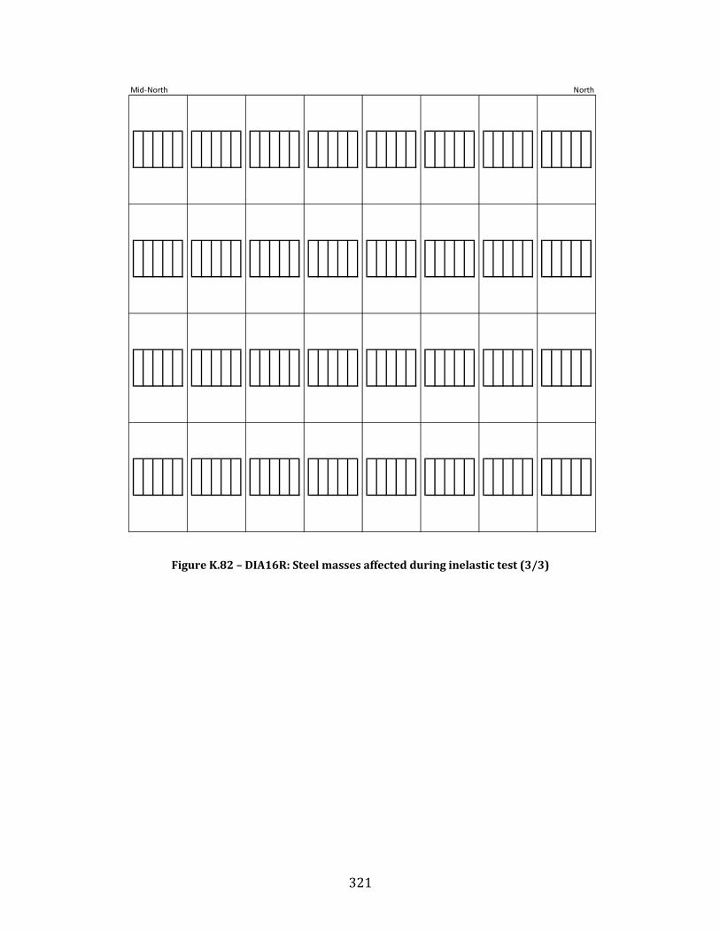
321

Figure K.82 – DIA16R: Steel masses affected during inelastic test (3/3)

Mid-North North

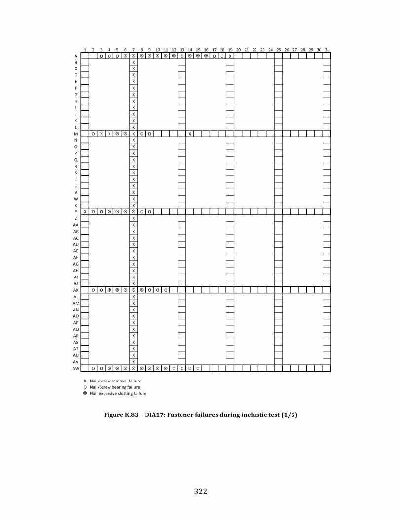
322

Figure K.83 – DIA17: Fastener failures during inelastic test (1/5)

1 2 3 4 5 6 7 8 9 10 11 12 13 14 15 16 17 18 19 20 21 22 23 24 25 26 27 28 29 30 31A O O O X O O XB XC XD XE XF XG XH XI XJ XK XL XM O X X X O O XN XO XP XQ XR XS XT XU XV XW XX XY X O O O OZ X

AA XAB XAC XAD XAE XAF XAG XAH XAI XAJ XAK O O O O OAL XAM XAN XAO XAP XAQ XAR XAS XAT XAU XAV XAW O O O X O O

X Nail/Screw removal failureO Nail/Screw bearing failure

Nail excessive slotting failure

323

Figure K.84 – DIA17: Fastener failures during inelastic test (2/5)

32 33 34 35 36 37 38 39 40 41 42 43 44 45 46 47 48 49 50 51 52 53 54 55 56 57 58 59 60 61

324

Figure K.85 – DIA17: Fastener failures during inelastic test (3/5)

62 63 64 65 66 67 68 69 70 71 72 73 74 75 76 77 78 79

325

Figure K.86 – DIA17: Fastener failures during inelastic test (4/5)

80 81 82 83 84 85 86 87 88 89 90 91 92 93 94 95 96 97 98 99 100 101 102 103 104 105 106 107 108 109

326

Figure K.87 – DIA17: Fastener failures during inelastic test (5/5)

110 111 112 113 114 115 116 117 118 119 120 121 122 123 124 125 126 127 128 129 130 131 132 133 134 135 136 137 138 139

X

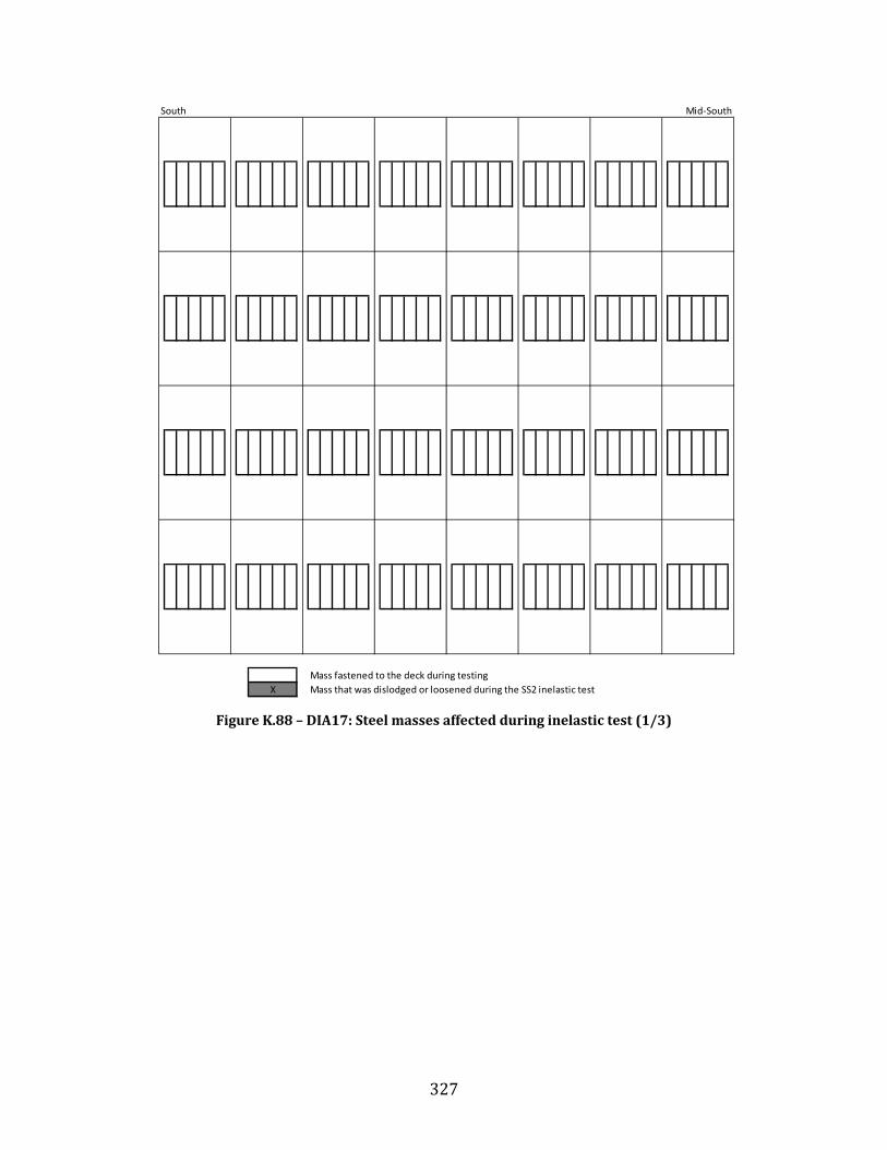
327

Figure K.88 – DIA17: Steel masses affected during inelastic test (1/3)

South Mid-South

Mass fastened to the deck during testingMass that was dislodged or loosened during the SS2 inelastic testX

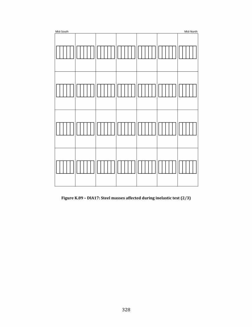
328

Figure K.89 – DIA17: Steel masses affected during inelastic test (2/3)

Mid-South Mid-North

329

Figure K.90 – DIA17: Steel masses affected during inelastic test (3/3)

Mid-North North

330

Figure K.91 – DIA17R: Fastener failures during inelastic test (1/5)

1 2 3 4 5 6 7 8 9 10 11 12 13 14 15 16 17 18 19 20 21 22 23 24 25 26 27 28 29 30 31XX

B XC XD XE XF XG XH OI OJK XL

N X OO XP XQ XR XS XT XU XV XW XX X O

XX

Z XAA XAB XAC XAD X OAE XAF XAG X OAH XAI XAJ X

XX

AL XAM X OAN XAO XAP XAQ XAR XAS XAT XAU XAV X

X XX X

X Nail/Screw removal failureO Nail/Screw bearing failure

Nail excessive slotting failure

A O O O XX X X

M O O X

Y O X O

AK O O X X O O O O

AW O O OX O

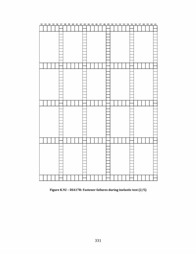
331

Figure K.92 – DIA17R: Fastener failures during inelastic test (2/5)

32 33 34 35 36 37 38 39 40 41 42 43 44 45 46 47 48 49 50 51 52 53 54 55 56 57 58 59 60 61

332

Figure K.93 – DIA17R: Fastener failures during inelastic test (3/5)

62 63 64 65 66 67 68 69 70 71 72 73 74 75 76 77 78 79

333

Figure K.94 – DIA17R: Fastener failures during inelastic test (4/5)

80 81 82 83 84 85 86 87 88 89 90 91 92 93 94 95 96 97 98 99 100 101 102 103 104 105 106 107 108 109

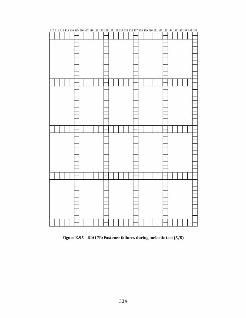
334

Figure K.95 – DIA17R: Fastener failures during inelastic test (5/5)

110 111 112 113 114 115 116 117 118 119 120 121 122 123 124 125 126 127 128 129 130 131 132 133 134 135 136 137 138 139

335

Figure K.96 – DIA17R: Steel masses affected during inelastic test (1/3)

South Mid-South

X

X

Mass fastened to the deck during testingMass that was dislodged or loosened during the SS2 inelastic testX

336

Figure K.97 – DIA17R: Steel masses affected during inelastic test (2/3)

Mid-South Mid-North

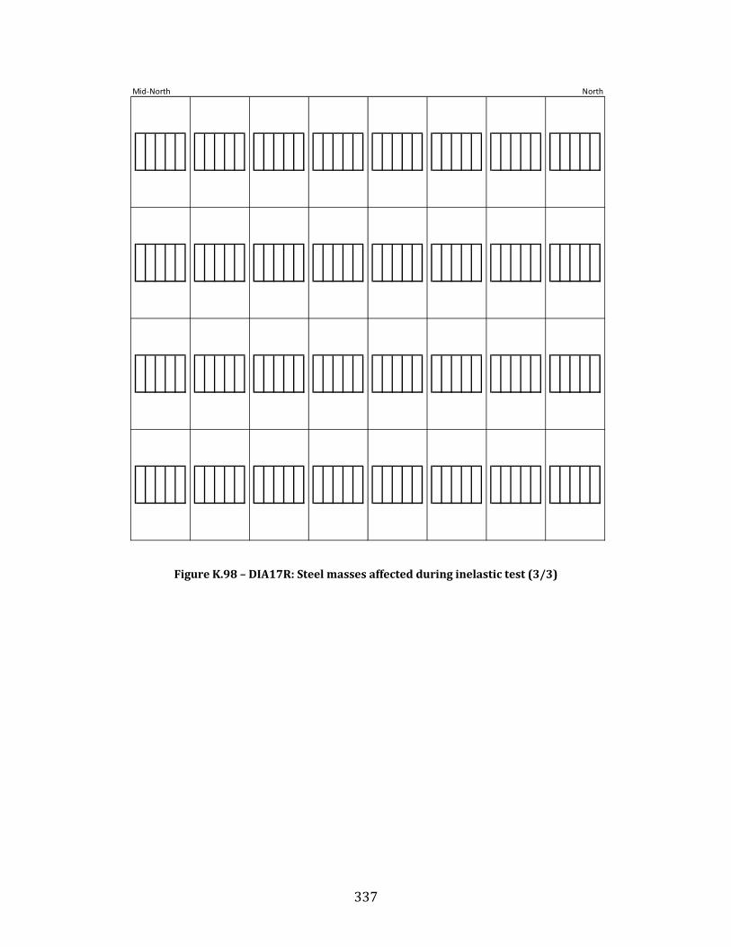
337

Figure K.98 – DIA17R: Steel masses affected during inelastic test (3/3)

Mid-North North

338

Figure K.99 – DIA18: Fastener failures during inelastic test (1/5)

1 2 3 4 5 6 7 8 9 10 11 12 13 14 15 16 17 18 19 20 21 22 23 24 25 26 27 28 29 30 31A O O OBCDEF OG OH O O OI O O OJ O OK O OL O OM O ONOP OQR X OSTU OVW OX OY O O OZ O O O

AA O O OAB O OAC O O OAD O O OAE OAF OAG OAHAIAJAK OAL OAM OAN OAO OAP O O OAQ O O OAR O OAS O OAT O OAU O OAVAW OAX OAY OAZBABBBCBDBE OBF OBG O O OBH O O OBI O OBJ O OBK O OBL O OBMBNBOBPBQ O O O O

X Nail/Screw removal failureO Nail/Screw bearing failure

Nail excessive slotting failure

O

O

O

O

O

O

O

O

O

O

O

O

O

O

O

O

O

O

O

O

O

O

O

O

O

O

O

O

O

O

O

O

O

O

O

O

O

O

O

O

O

O

O

O

O

O

O

O

O

O

O

O

O

O

O

O

O

O

O

O

O

O

O

O

O

O

O

O

O

O

O

O

O

O

O

O

O

O

O

O

O

O

O

O

O

O

O

O

O

O

O

O

O

O

O

O

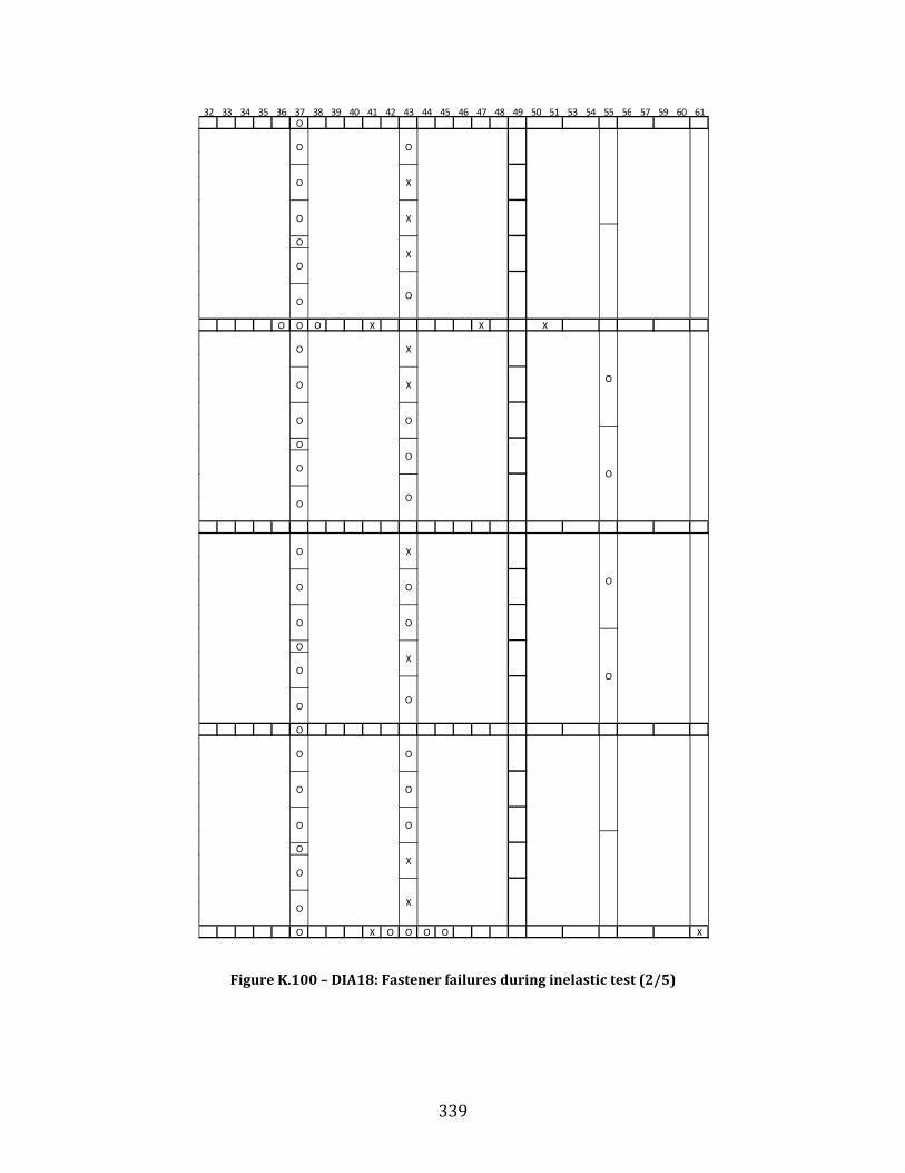
339

Figure K.100 – DIA18: Fastener failures during inelastic test (2/5)

32 33 34 35 36 37 38 39 40 41 42 43 44 45 46 47 48 49 50 51 53 54 55 56 57 59 60 61O

O

O O O X X

O

O

O

O

O X O O O O X

O

O

O

O

O

O

O

O

O

O

O

O

O

O

O

O

O

O

O

O

O

O

X

O

X

X

X

X

O

X

O

O

O

X

X

O

O

X

O

O

O

O

O

O

X

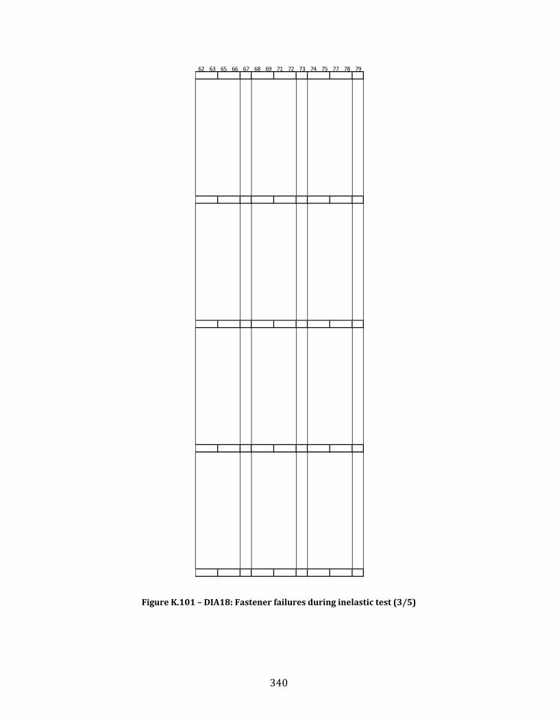
340

Figure K.101 – DIA18: Fastener failures during inelastic test (3/5)

62 63 65 66 67 68 69 71 72 73 74 75 77 78 79

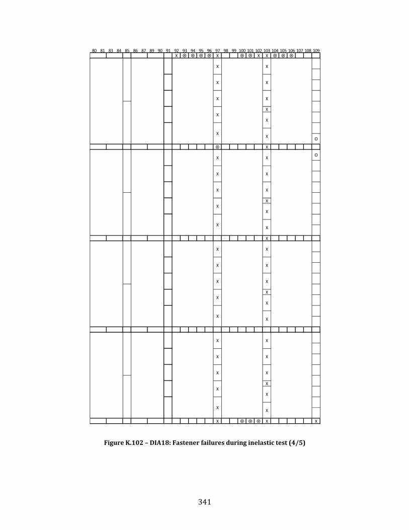
341

Figure K.102 – DIA18: Fastener failures during inelastic test (4/5)

80 81 83 84 85 86 87 89 90 91 92 93 94 95 96 97 98 99 100 101 102 103 104 105 106 107 108 109X X X X

X

X

X

X

X

X

X X X

X

X

X

X

X

X

X

X

X

X

X

X

X

X

X

X

X

X

X

X

X

X

X

X

X

X

X

X

X

X

O

OX

X

X

X

X

X

X

X

X

X

342

Figure K.103 – DIA18: Fastener failures during inelastic test (5/5)

110 111 112 113 114 115 116 117 118 119 120 115 122 123 124 125 126 127 128 129 130 131 132 133 134 135 136 137 138 139

X

X X

O

X X X X

O

O

343

Figure K.104 – DIA18: Steel masses affected during inelastic test (1/3)

South Mid-South

Mass fastened to the deck during testingMass that was dislodged or loosened during the SS2 inelastic testX

344

Figure K.105 – DIA18: Steel masses affected during inelastic test (2/3)

Mid-South Mid-North

X

345

Figure K.106 – DIA18: Steel masses affected during inelastic test (3/3)

Mid-North North

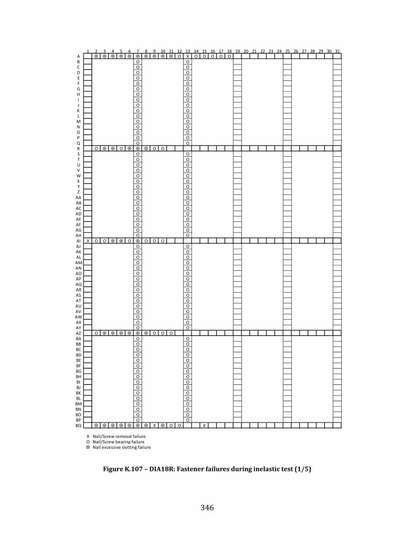
346

Figure K.107 – DIA18R: Fastener failures during inelastic test (1/5)

1 2 3 4 5 6 7 8 9 10 11 12 13 14 15 16 17 18 19 20 21 22 23 24 25 26 27 28 29 30 31A O X O O O O OB O OC O OD O OE O OF O OG O OH O OI O OJ O OK O OL O OM O ON O OO O OP O OQ O OR O O O OS O OT O OU O OV O OW O OX O OY O OZ O O

AA O OAB O OAC O OAD O OAE O OAF O OAG O OAH O OAI X O O O O O OAJ O OAK O OAL O OAM O OAN O OAO O OAP O OAQ O OAR O OAS O OAT O OAU O OAV O OAW O OAX O OAY O OAZ O O O OBA O OBB O OBC O OBD O OBE O OBF O OBG O OBH O OBI O OBJ O OBK O OBL O OBM O OBN O OBO O OBP O OBQ X O O X

X Nail/Screw removal failureO Nail/Screw bearing failure

Nail excessive slotting failure

347

Figure K.108 – DIA18R: Fastener failures during inelastic test (2/5)

32 33 34 35 36 37 38 39 40 41 42 43 44 45 46 47 48 49 50 51 52 53 54 55 56 57 58 59 60 61

348

Figure K.109 – DIA18R: Fastener failures during inelastic test (3/5)

62 63 64 65 66 67 68 69 70 71 72 73 74 75 76 77 78 79

349

Figure K.110 – DIA18R: Fastener failures during inelastic test (4/5)

80 81 82 83 84 85 86 87 88 89 90 91 92 93 94 95 96 97 98 99 100 101 102 103 104 105 106 107 108 109

X

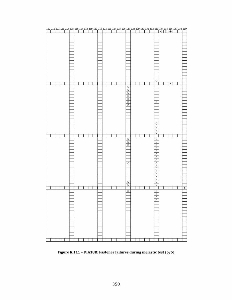
350

Figure K.111 – DIA18R: Fastener failures during inelastic test (5/5)

110 111 112 113 114 115 116 117 118 119 120 115 122 123 124 125 126 127 128 129 130 131 132 133 134 135 136 137 138 139O

OX

OOOOOO OO

OOOO

O OO OO O

OOOOO

O OOOOOO

O OO O

XO O

OOO

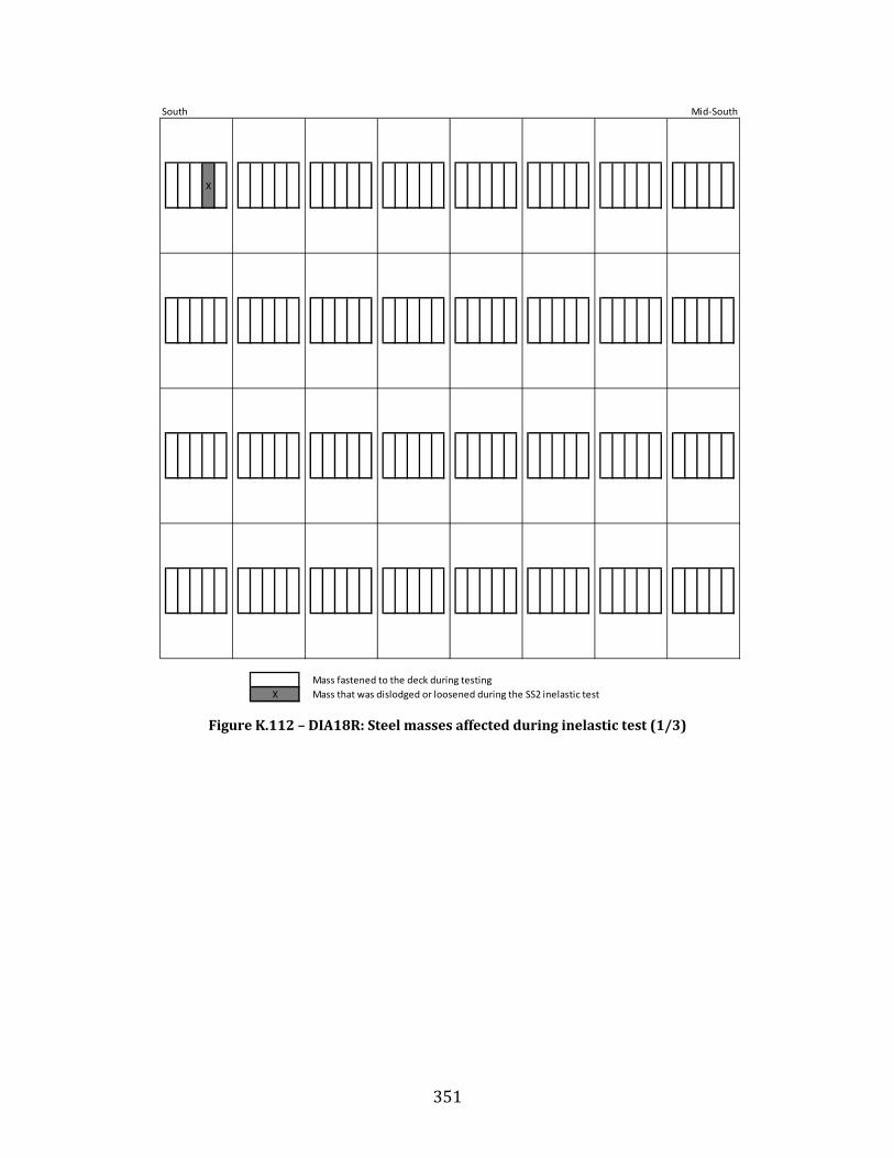
351

Figure K.112 – DIA18R: Steel masses affected during inelastic test (1/3)

South Mid-South

X

Mass fastened to the deck during testingMass that was dislodged or loosened during the SS2 inelastic testX

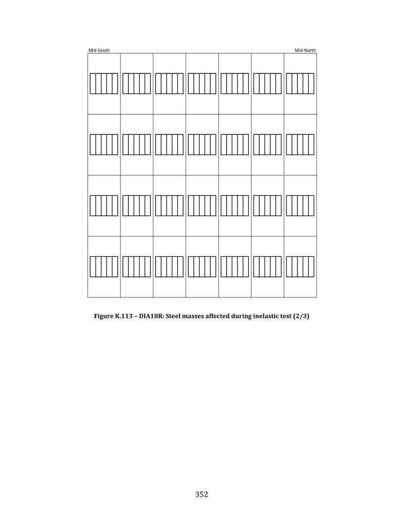
352

Figure K.113 – DIA18R: Steel masses affected during inelastic test (2/3)

Mid-South Mid-North

353

Figure K.114 – DIA18R: Steel masses affected during inelastic test (3/3)

Mid-North North

354

Figure K.115 – DIA19: Fastener failures during inelastic test (1/5)

1 2 3 4 5 6 7 8 9 10 11 12 13 14 15 16 17 18 19 20 21 22 23 24 25 26 27 28 29 30 31AB OC OD OE OF OGH OIJ O OK O OL OMN O OO O OP O OQ ORST OU O OV O OW O OX O OYZ O O

AA O OAB O OAC OAD OAE OAF O OAG O OAH O OAI O OAJ O OAKAL O OAM O OAN OAO O OAP O OAQ O OAR O OAS OAT OAU O OAV O OAW

X Weld popping/Screw removal failureO Weld/Screw bearing failure

355

Figure K.116 – DIA19: Fastener failures during inelastic test (2/5)

32 33 34 35 36 37 38 39 40 41 42 43 44 45 46 47 48 49 50 51 52 53 54 55 56 57 58 59 60 61

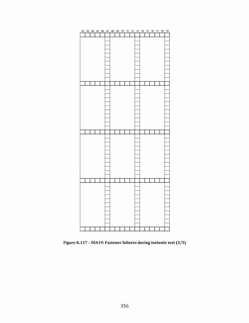
356

Figure K.117 – DIA19: Fastener failures during inelastic test (3/5)

62 63 64 65 66 67 68 69 70 71 72 73 74 75 76 77 78 79

357

Figure K.118 – DIA19: Fastener failures during inelastic test (4/5)

80 81 82 83 84 85 86 87 88 89 90 91 92 93 94 95 96 97 98 99 100 101 102 103 104 105 106 107 108 109

358

Figure K.119 – DIA19: Fastener failures during inelastic test (5/5)

110 111 112 113 114 115 116 117 118 119 120 121 122 123 124 125 126 127 128 129 130 131 132 133 134 135 136 137 138 139X X X X XXXXXX

O XXXXXXX X X XXXXXXXX

O XO X

XXX X X X

O XO XO XO X

XXXXXXXX X XXXXXXXXXXXXX X X X X

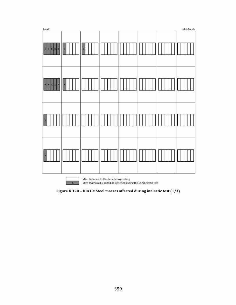
359

Figure K.120 – DIA19: Steel masses affected during inelastic test (1/3)

South Mid-South

X X X X X X X

X X X X X X

X

X

Mass fastened to the deck during testingMass that was dislodged or loosened during the SS2 inelastic testX

360

Figure K.121 – DIA19: Steel masses affected during inelastic test (2/3)

Mid-South Mid-North

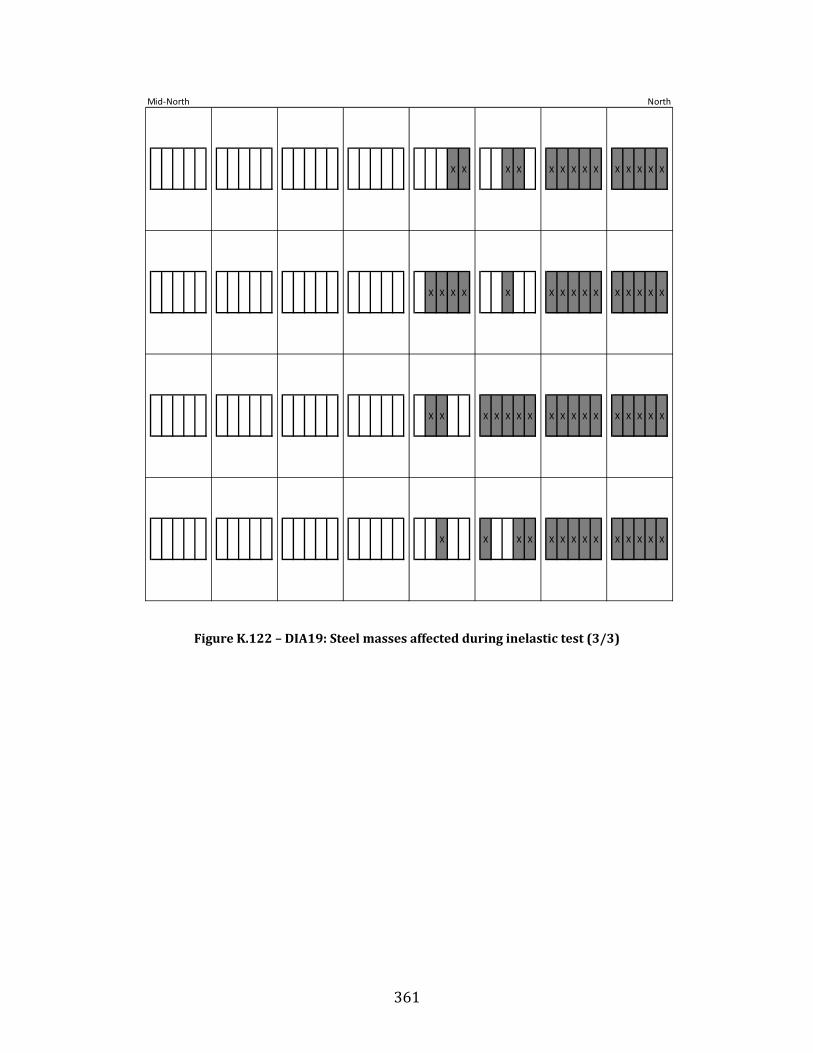
361

Figure K.122 – DIA19: Steel masses affected during inelastic test (3/3)

Mid-North North

X X X X X X X X X X X X X X

X X X X X X X X X X X X X X X

X X X X X X X X X X X X X X X X X

X X X X X X X X X X X X X X

362

Figure K.123 – DIA19R: Fastener failures during inelastic test (1/5)

1 2 3 4 5 6 7 8 9 10 11 12 13 14 15 16 17 18 19 20 21 22 23 24 25 26 27 28 29 30 31ABCDEFGHIJKLMNOPQRSTUVWXYZ

AAABACADAEAFAGAHAIAJ OAK XALAMANAOAPAQARASATAUAVAW

X Nail/Screw removal failure Y Weld fracture failureO Nail/Screw bearing failure P Weld bearing failure

363

Figure K.124 – DIA19R: Fastener failures during inelastic test (2/5)

32 33 34 35 36 37 38 39 40 41 42 43 44 45 46 47 48 49 50 51 52 53 54 55 56 57 58 59 60 61

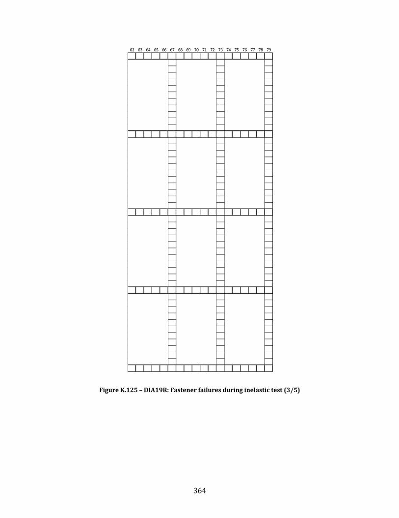
364

Figure K.125 – DIA19R: Fastener failures during inelastic test (3/5)

62 63 64 65 66 67 68 69 70 71 72 73 74 75 76 77 78 79

365

Figure K.126 – DIA19R: Fastener failures during inelastic test (4/5)

80 81 82 83 84 85 86 87 88 89 90 91 92 93 94 95 96 97 98 99 100 101 102 103 104 105 106 107 108 109

366

Figure K.127 – DIA19R: Fastener failures during inelastic test (5/5)

110 111 112 113 114 115 116 117 118 119 120 121 122 123 124 125 126 127 128 129 130 131 132 133 134 135 136 137 138 139XY XY XY XY XY XY XY XY XY XY XY

XXXXXXXXXXX

Y XY XY XY XY XY OYXXXXXXXXXXX

Y Y Y XY XY XY XY OY OYXXXXXXXXXXX

Y XY XY XY XY XY XY OYXXXXXXXXXXX

XY XY XY XY XY XY XY XY XY XY XY OY

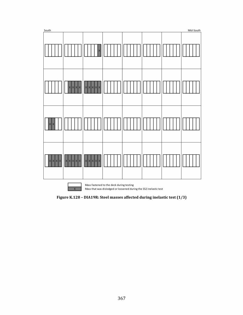
367

Figure K.128 – DIA19R: Steel masses affected during inelastic test (1/3)

South Mid-South

X

X X X X X X X X X

X X

X X X X X X X X X X X X X X

Mass fastened to the deck during testingMass that was dislodged or loosened during the SS2 inelastic testX

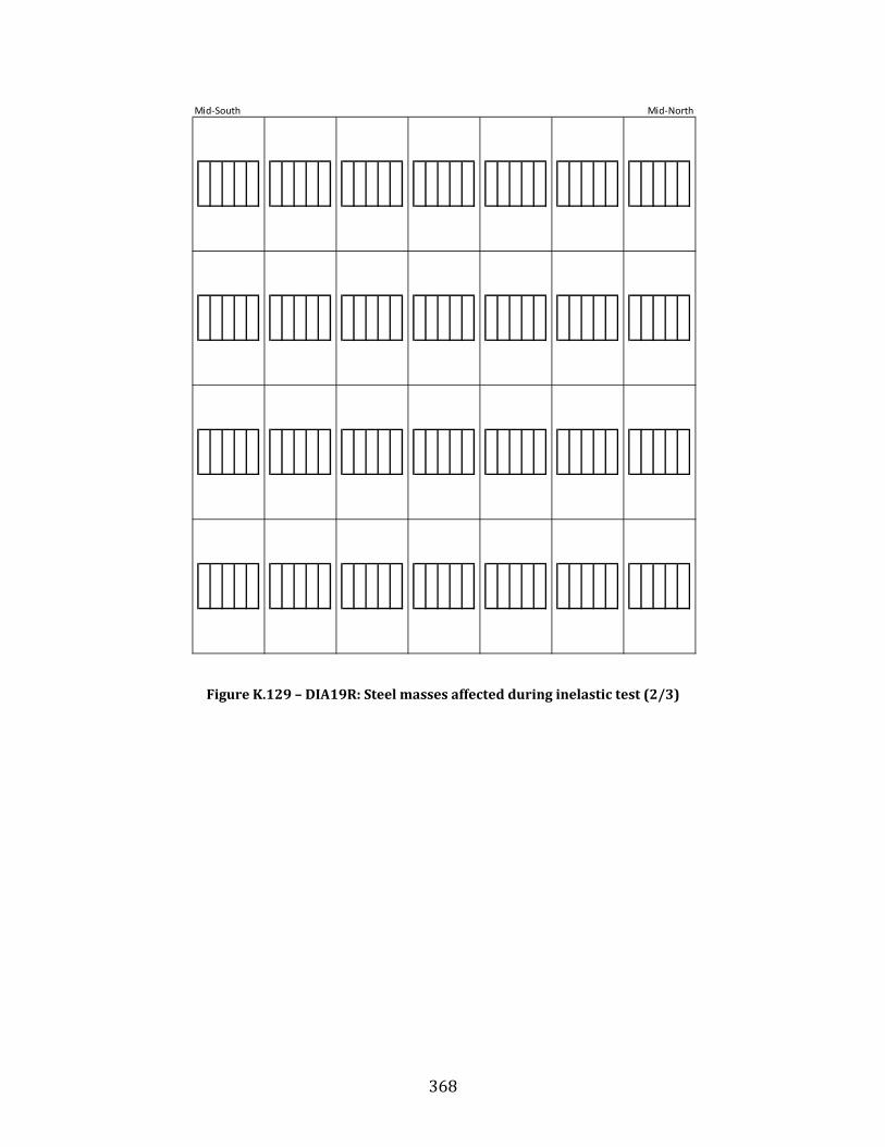
368

Figure K.129 – DIA19R: Steel masses affected during inelastic test (2/3)

Mid-South Mid-North

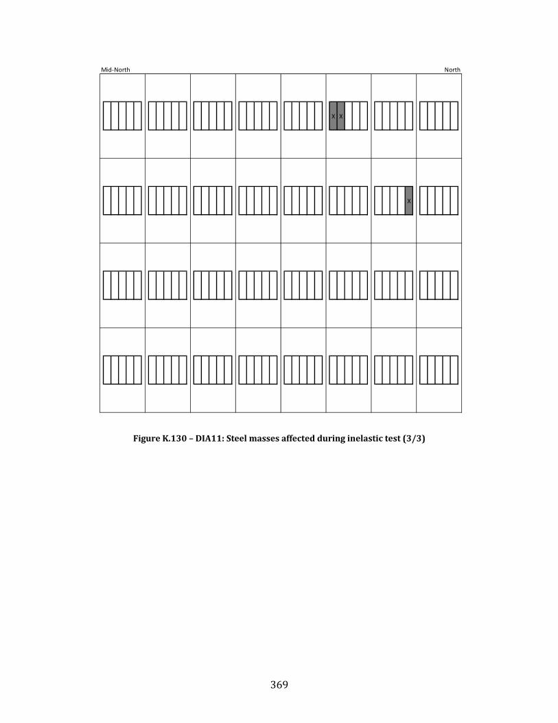
369

Figure K.130 – DIA11: Steel masses affected during inelastic test (3/3)

Mid-North North

X X

X

370

Appendix L:

STIFFNESS, STRENGTH, AND INELASTIC PROPERTY GRAPHS FOR

ALL NEW PHASE I, II AND III DIAPHRAGM SPECIMENS

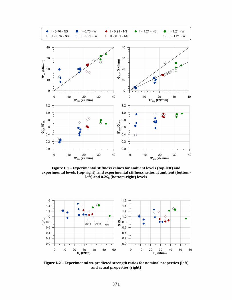
371

Figure L.1 – Experimental stiffness values for ambient levels (top-left) and

experimental levels (top-right), and experimental stiffness ratios at ambient (bottom-left) and 0.2Sn (bottom-right) levels

Figure L.2 – Experimental vs. predicted strength ratios for nominal properties (left)

and actual properties (right)

I - 0.76 - WII - 0.76 - W

I - 0.76 - NSII - 0.76 - NS

I - 1.21 - NS I - 1.21 - WII - 1.21 - W

I - 0.91 - NSII - 0.91 - NS

0 10 20 30 40G'SDI (kN/mm)

0.0

0.2

0.4

0.6

0.8

1.0

1.2

G' EX

P/G' 20

%

0 10 20 30 40G'SDI (kN/mm)

0.0

0.2

0.4

0.6

0.8

1.0

1.2

G' EX

P/G' 0%

0 10 20 30 40G'SDI (kN/mm)

0

10

20

30

40

G' EX

P (kN

/mm

)

0 10 20 30 40G'SDI (kN/mm)

0

10

20

30

40G

' 0% (k

N/m

m)

1:11:1

0.67:1

0 10 20 30 40 50 60Sn (kN/m)

0.0

0.2

0.4

0.6

0.8

1.0

1.2

1.4

1.6

S u/S

na

0 10 20 30 40 50 60Sn (kN/m)

0.0

0.2

0.4

0.6

0.8

1.0

1.2

1.4

1.6

S u/S

n

36/11 36/11 36/9

372

Figure L.3 – Distance to the centre-of-damage, xfailure, measured from the end beam for

new and repaired specimens

Figure L.4 – γu (top-left), γp (top-right), γu/γy (bottom-left) and normalized energy dissipated (bottom-right) as a function of predicted strength

I - 0.76 - WII - 0.76 - W

I - 0.76 - NSII - 0.76 - NS

I - 1.21 - NS I - 1.21 - WII - 1.21 - W

I - 0.91 - NSII - 0.91 - NS

0 10 20 30 40 50 60Sn (kN/m)

0.0

1.0

2.0

3.0

4.0

x fai

lure

(m)

0

5

10

15

x fai

lure

/ L

(%)

0 10 20 30 40 50 60Sn (kN/m)

0.0

0.1

0.2

0.3

0.4

Nor

mal

ized

Ene

rgy

Dis

sipa

ted

0 10 20 30 40 50 60Sn (kN/m)

0

1

2

3

4

5

6

γ u/γ y

0 10 20 30 40 50 60Sn (kN/m)

02468

101214161820

γ p (m

Rad

)

0 10 20 30 40 50 60Sn (kN/m)

02468

101214161820

γ u (m

Rad

)