Dynamic behavior of direct spring loaded pressure relief

valves in gas service: model development, measurements

and instability mechanismsI

C.J. Hosa, A.R. Champneysb, K. Paulc, M. McNeelyc

aDepartment of Hydrodynamic Systems, Budapest University of Technology andEconomics, 1111 Budapest, Muegyetem rkp. 3. Budapest, Hungary

bDepartment of Engineering Mathematics, University of Bristol, Queen’s Building BristolBS8 1TR, UK

cPentair Valves and Controls, 3950 Greenbriar Drive, Stafford, TX 77477, USA

Abstract

A synthesis of previous literature is used to derive a model of an in-servicedirect-spring pressure relief valve. The model couples low-order rigid bodymechanics for the valve to one-dimensional gas dynamics within the pipe.Detailed laboratory experiments are also presented for three different com-mercially available values, for varying mass flow rates and length of inletpipe. In each case, violent oscillation is found to occur beyond a critical pipelength, which may be triggered either on valve opening or closing. The testresults compare favorably to the simulations using the model. In particu-lar, the model reveals that the mechanism of instability is a Hopf bifurcation(flutter instability) involving the fundamental, quarter-wave pipe mode. Fur-thermore, the concept of the effective area of the valve as a function of valvelift is shown to be useful in explaining sudden jumps observed in the testdata. It is argued that these instabilities are not alleviated by the 3% inletline loss criterion that has recently been proposed as an industry standard.

Keywords:pressure-relief valve, gas dynamics, instability, quarter-wave, Hopfbifurcation, flutter, chatter

IShort title: Dynamics of gas pressure relief valves

Preprint submitted to Journal of Loss Prevention in the Process IndustriesOctober 27, 2015

CORE Metadata, citation and similar papers at core.ac.uk

Provided by Repository of the Academy's Library

Contents

1 Introduction 3

2 Model development 72.1 Valve body dynamics . . . . . . . . . . . . . . . . . . . . . . . 82.2 Reservoir dynamics and discharge flow rate . . . . . . . . . . . 92.3 Pipeline dynamics . . . . . . . . . . . . . . . . . . . . . . . . . 122.4 Solution technique . . . . . . . . . . . . . . . . . . . . . . . . 13

3 Experimental results and model validation 133.1 Experimental set-up . . . . . . . . . . . . . . . . . . . . . . . 143.2 Test results . . . . . . . . . . . . . . . . . . . . . . . . . . . . 153.3 Comparison with simulations . . . . . . . . . . . . . . . . . . 20

4 Identification of instability mechanisms 214.1 Valve jumps . . . . . . . . . . . . . . . . . . . . . . . . . . . . 214.2 Flutter and chatter . . . . . . . . . . . . . . . . . . . . . . . . 244.3 Cycling and the 3% inlet pressure loss criterion . . . . . . . . 244.4 Stability charts . . . . . . . . . . . . . . . . . . . . . . . . . . 28

5 Summary and outlook 30

2

1. Introduction

This paper summarizes and extends recent scientific investigations intothe mechanisms of instability in pressure relief valves (PRVs) and considerstheir implications for practical operation. The overall aim is to develop anew comprehensive understanding of the issues that affect valve stabilityin operation, in order to influence a new set of design guidelines for theiroperation and manufacture. In particular we shall combine theoretical modelstudies with tests of fully instrumented valves within representative pipegeometries. This paper will focus specifically on direct spring-loaded PRVs ingas service, particularly considering the combined effect of the valve dynamicswith acoustic pressure waves within its inlet pipe.

A considerable amount of scientific literature has been published on thedescription and analysis of valve systems. Green and Woods (1973) providedthe first comprehensive discussion of the possible causes of valve instabili-ties, suggesting that they can be induced as a result of five different effects:the interaction between the poppet and other elements, flow transition fromlaminar to turbulent during opening and closing, a negative restoring force,hysteresis of the fluid force, and fluctuating supply pressure. This paper shallfocus on the first of these, specifically instability due to interaction betweenthe valve and the inlet pipe (although, as we shall see, this can also be in-terpreted as an effective negative restoring force on the valve provided byan acoustic wave). Instabilities due to the other four effects identified byGreen and Woods have been analyzed by a number of other authors (Kasai,1968; McCloy and McGuigan, 1964; Madea, 1970a,b; Nayfeh and Bouguerra,1990; Vaughan et al., 1992; Moussou et al., 2010; Beune, 2009; Song et al.,2011). Conventional PRVs subject to built-up back pressure have also beenwidely investigated (Francis and Betts, 1998; Chabane et al., 2009; Moussouet al., 2010). In this paper we do not consider effects of downstream piping.Oscillations in other valve systems have also been studied, e.g. in plug valves(D’Netto and Weaver, 1987), compressor valves (Habing and Peters, 2006),ball valves (Nayfeh and Bouguerra, 1990), pilot-operated two-stage valves(Botros et al., 1997; Zung and Perng, 2002; Ye and Chen, 2009) and controlvalves (Misra et al., 2002). Again, such studies go beyond the scope of thepresent work.

The first serious discussion of self-excited instabilities of poppet valvesemerged in the 1960s. Funk (1964) discussed the influence of valve chambervolume and pipe length within a hydraulic circuit on the stability of a pop-

3

pet valve. He found that such valves are inclined to become unstable at acritical frequency that coincides with the fundamental vibratory mode of thepipeline. Moreover, the severity of the instability increases with the lengthof the pipe. Kasai (1968) developed this analysis by deriving equations ofmotion for such a poppet valve and inlet piping system. Based on linear sta-bility analysis, he established formulas for predicting instability in the valve.The results were shown to be in broad agreement with experiments. A sim-ilar configuration was studied by Thomann (1976) who found that the valvemotion can couple to the acoustic oscillation of the pipe, leading to amplifiedoscillation of the system. He also developed analytical criteria for the loss ofstability, finding good agreement with experiments. Later, MacLeod (1985)developed a model that includes gas dynamical issues such as choked flowcapable of predicting the region of stable operation of a simple spring loadedPRV mounted directly onto a gas-filled pressure vessel.

In the 1990s Hayashi (1995) and Hayashi et al. (1997) carried out detailedlinear and global stability analyses of a poppet valve circuit and showed rep-resentative examples of ’soft’ and ’hard’ self-excited vibration. They revealedthat for the same conditions several pipe vibration modes can become simul-taneously unstable, with the number of unstable modes increasing with pipelength. These results agree with those obtained by Botros et al. (1997) whofind that for higher values of the pipe length two modes evolve in the systemwhile for lower values of the pipe length the vibration is primarily in the fun-damental, quarter-wave mode. They also found that maximum amplitudeoccurs when the oscillation frequency coincides with the quarter-wave natu-ral frequency; for lower and higher values of the pipe length the amplitudedecreases.

In early work by two of us (Licsko et al., 2009), we used nonlinear dynam-ical systems methods to analyze a low-order system of ordinary differentialequations describing a simplified version of the set up used by Kasai (1968)and Hayashi et al. (1997), ignoring the effect of the pipe. Here we showedthat upon reduction of the inlet flow rate, loss of stability is due to a Hopfbifurcation (also known as a flutter instability in aeroelastics) is initiated bya so-called self-excited oscillation; a dynamic instability which is present inthe system even in the absence of explicit external excitation. The systemwas further investigated by Hos and Champneys (2012), where we elucidatedthe nature of grazing bifurcations in the system that underlie the onset ofimpacting motion between the valve and its seat, and performed detailed two-parameter continuation. At the same time, Bazso and Hos (2013a) report

4

experimental results in a hydraulic system that showed qualitative agreementto the nonlinear dynamics predicted by Licsko et al. (2009). That paper alsopresented a preliminary stability map that shows the frequency of the evolv-ing self-excited vibration along the boundary of loss of stability, again forhydraulic application. Furthermore, Bazso et al. (2013b) provide a detailedmathematical derivation of the model studied here in section 2, which ex-tends the reduced-order model of Licsko et al. (2009) to include the morerealistic effects of a downstream inlet pipe. The present paper though is thethe first to compare that model with experimental data and to consider thepractical application of the findings of the model. It should be noted thatour model and conclusions bear similarities with that used in the study byIzuchi (2010). Our work though has far more detailed test data and we havealso identified the key parameters and mechanisms affecting instability.

In parallel to the scientific literature, there has been industry-fundedstudies into the safe operation of pressure relief systems. For example, theAmerican Institute of Chemical Engineering (AIChE) founded in 1976 theDesign Institute for Emergency Relief Systems (DIERS) whose twin aims arethe reduce pressure producing accidents and to develop new techniques toimprove the design of relief systems. Meanwhile, the American PetroleumInstitute (API) have funded their own internal program into the causes ofPRV instability. Many of their findings are included in the draft 6th editionof API standard RP520 Part II. In particular, the standard is careful topoint out the difference between valves undergoing three different types ofbehaviour, all of which have previously been referred to as instability. Theseare

1. cycling,

2. valve flutter, and

3. valve chatter.

Here, cycling refers to a valve that opens and closes multiple times during apressure-relief event. Typically this behaviour is of low frequency (< 1Hz)and can be caused either by valve oversizing or inlet pressure loss causingthe pressure to drop transiently, and the valve to shut. As pressure buildsup again, the valve re-opens, with this chain of events happening repeatedly.In contrast, flutter is a high-frequency self-excited periodic oscillation of thevalve (typically > 10Hz) that does not result in the valve completely closingoff. Finally, chatter is a more violent form of rapid oscillatory motion thatinvolves the valve repeatedly impacting with its seat at high frequency. The

5

API RP520 standard is less clear on the precise causes of flutter or chatter-ing instability mechanisms, but resonant coupling between the valve and itspipework, or instabilities being triggered from periodically shed vortices havebeen postulated as possible causes of flutter.

One of the aims of this paper is to explain these three phenomena interms used in the recent scientific literature. In particular, we shall showthat the onset of flutter can be regarded as a Hopf bifurcation (which isalso commonly known as flutter in the aeroelastic research community). Asshown in detail in simplified models (Licsko et al., 2009; Hos and Champneys,2012), chatter often arises as the amplitude of the limit cycle resulting froma Hopf bifurcation grows to the extent that the valve body touches the valveseat. This causes a so-called grazing bifurcation that causes the onset ofmore violent, repeatedly impacting motion. Cycling behaviour is, as we havementioned, better understood industrially and is not the subject of this paperper se. Nevertheless we do show in Section 4.3 below that our mathematicalmodel is capable of reproducing this behaviour.

To avoid cycling, the API standard proposes that the line pressure lossshould be less than 3% of the set pressure. However, as we shall see, thisis not sufficient to prevent self-excited flutter or chatter instabilities in thevalves we have tested.

The remainder of this paper is outlined as follows. First, Sec. 2 presents amathematical model that combines the rigid-body dynamics of a direct springvalve with 1D gas dynamics within the pipe. The valve model is sufficientlycomplex to consider realistic valve design parameters such as set pressureand a prescribed relation between the effective valve area and the valve’slift. Then, in Sec. 3 we present a detailed validation of the model againsttest data performed on three different commercially available valves. In eachcase we run a pressure run-up and run-down event for for several differentmass flow rates and inlet pipe lengths. A detailed comparison between modeland data is presented, and close agreement is found for both the nature ofthe instabilities observed and for the flow rates and pipe lengths for whichinstability is triggered. This leads to a detailed discussion in Sec. 4 whichidentifies the possibility of dynamic jumps due to steepness of the effectivearea versus lift curves, and the origin of cycling, flutter and chatter. Theseterms are also explained using the language of nonlinear dynamical systemstheory, in order to provide a link between the practical engineering literatureand more scientific studies. Finally, Sec. 5 provides a summary, includingsome tentative conclusions on how instability may be prevented in future,

6

Figure 1: Definition sketch of the mathematical model

and gives an outlook to the results of future studies.

2. Model development

Consider the system depicted in Fig. 1 consisting of a reservoir, a pipeand a direct spring-loaded valve. The reservoir is taken to be perfectly rigidwith volume V , pressure pr (that might vary in time) and temperature Tr.The mass flow rate mr,in of the compressible fluid entering the reservoir ispresumed either to be constant or to vary slowly when compared to othertimescales present in the system (notably valve and pipe eigenfrequencies ).The change of state in the reservoir is assumed to be isentropic, that is, thereis no heat exchange with the surroundings and there are no internal losses.The mass outflow from the reservoir is in general assumed to be time varying.

The flow in the long, thin pipe with diameter D, length L and friction fac-tor f is assumed to be captured by one-dimensional unsteady gas-dynamicstheory, including the effects of wall friction. Such an approach captures theinertia of the fluid, its compressibility and pressure losses, which allows forthe presence of both wave effects and damping.

The valve body is modeled as a single degree-of-freedom oscillator thatobeys a Newtonian equation of motion. The mass of the moving parts is m,the spring constant is s, the viscous damping coefficient is k. The set pressure

7

is adjusted by varying the spring pre-compression x0. The pipe pressure closeto the valve body will be denoted by pv, which is in general time-dependent.In contrast we assume constant back-pressure p0 behind the valve.

2.1. Valve body dynamics

The valve itself consists of an inertial mass, the valve body, and a pre-compressed spring. The motion of such PRVs are usually very weakly damped.Nevertheless, we shall include some very low, nearly zero viscous dampingin the model to represent the internal damping of the spring and the dragand added-mass effect of the fluid, see e.g. (Khalak and Williamson, 1997;Askari et al., 2013). The motion of the valve disk can be described as asingle degree-of-freedom rigid body, with mass m, spring constant s and vis-cous damping with coefficient k. The pre-compression of the spring will bedenoted by x0 while xv stands for the displacement of the valve disk. Thegoverning equation is thus given by

mxv + kxv + s(x0 + xv) = Ffluid(xv, pv), for xv > 0, (1)

where a dot represents differentiation with respect to time.The fluid force consists of two parts: pressure force and momentum force

due to the deflection of the fluid jet, see the left-hand side of Figure 2. Wehave

Ffluid(xv, pv) = pvA+ m (vf,v + vf,j cos β) , (2)

where pv is the pressure beneath the valve, A = D2π/4 is the pipe cross-section, m is the mass flow rate through the valve, vf,v and vf,j are the meanfluid velocities in the pipe and in the jet, respectively, and β is the jet angle.We assume that the density change is negligible between the valve end ofthe pipe and jet, hence m = ρvAvf,v = ρvAft(xv)vf,j with Aft(xv) = Dπxvbeing the valve flow-through area (see Figure 2 for details). Upon using thestandard choked discharge equation (6) (see the next sub-section for details),we have

Ffluid(xv, pv) = pvA

(1 + c2C2

d

Aft(xv)

A

(Aft(xv)

A+ cos β

)):= pvAeff(xv)

(3)The function Aeff will be referred to as effective area, which is defined as

the force on the valve divided by the fluid pressure pv. Introducing this quan-tity enables us to combine the pressure and momentum force into a single

8

expression, thus greatly simplifying the analysis. However, analytical esti-mation based on (3) requires a priori knowledge of the flow deflection angleβ, which is highly non-trivial and depends not only on the valve geometrybut also on the valve lift. Moreover, the effective area is likely to be a de-tailed function of the valve’s geometry, (blow down rings, huddling chamberor shroud, etc.) and the fluid mechanics within the valve’s orifices. We havefound it convenient to characterize a valve by the variation of this effectivearea with valve lift. As we shall see, the stability of a valve can be greatlyaffected by the shape of this effective-area versus lift curve, which can bemeasured or computed by means of CFD as in Bazso and Hos (2013b)) foreach individual valve. See, for example, the right-hand side of Fig. 2 for aschematic or Fig. 11 below for an actual measured effective area curve).

Once the valve body hits the seat, i.e. when xv = 0 with xv < 0, we applythe impact law

x+v = −rx−v , (4)

where x±v are the valve velocities immediately before and after the impactand r is a coefficient of restitution.

On the other hand, if the valve is closed xv = 0 and the mean flow in thepipe is zero (so that xv = 0 and xv = 0), the reservoir pressure at which thevalve opens, the so-called set pressure, is given by

pset =sx0

Aeff(0)+ p0 . (5)

2.2. Reservoir dynamics and discharge flow rate

When modeling the fluid dynamics in the orifice (i.e. at the valve) andthe reservoir pressure dynamics, we should keep in mind that we are tryingto capture the behaviour of PRVs. Such valves are only designed to openwhen there is a significant pressure difference between the upstream pressureand the downstream pressure, as given by (5). It is therefore reasonable toassume that this difference is large enough for choked flow to occur. Thismeans that flow reaches the sonic velocity at the narrowest cross section, theso-called vena contracta and hence the downstream pressure does not affectthe flow rate; for details, see Zucrow and Hoffman (1976).

As an illustration to quantify when such a choked flow assumption is valid,consider the case of air, whose specific heat ratio is κ = 1.4. Straightforwardcalculations reveal that choking occurs if the pressure ratio pv

p0is greater than

1.893, which is clearly the case for pressure relief devices used in practice.

9

prv_zoom_and_Aeff.pdf

Figure 2: The momentum force on the valve (left) and a typical effective area curve (right);notice the rapid increase close to zero lift which is indicative of the blowdown effect of thevalve.

10

Note that we do not assume that back-pressure is necessarily ambient, merelythat it is constant.

The mass flow rate through the valve is given by

m = CdAft(xv) c√ρv pv, (6)

where Cd is the empirically derived discharge coefficient,

c =

√κ

(2

κ+ 1

)κ+1κ−1

(7)

and κ is the gas’s heat capacity ratio. And Aft is the valve’s flow througharea which unlike the effective area, is a pure function of geometry, which wewrite as

Aft = Dπxv,

The imbalance between the inflow and outflow rates results in a changein the reservoir pressure. We assume that the fluid obeys the ideal gaslaw, p/ρ = RT , and that the process in the reservoir is isentropic, p/ρκ =constant. Mass balance in the reservoir of volume V therefore gives

dm

dt= V

d

dt(ρr(t)) = V

d

dt

(p(t)

RT (t)

)= min − mout (8)

Given an ambient reference state p0, T0, the temperature can be related tothe pressure via

T (t) = T0

(pr(t))

p0

)κ−1κ

, (9)

which gives

pr = κRT0

V

(prp0

)κ−1κ

(min − mout) =a2

V(min − mout) , (10)

with a =√κRT being the sonic velocity associated with the reservoir tem-

perature T .

11

2.3. Pipeline dynamics

The flow inside the pipe is assumed to be compressible, one-dimensionaland any pressure loss can be attributed to wall friction. The gas is assumedto be ideal but the change of state is not fixed hence, besides the usualcontinuity and momentum equations of gas dynamics, we also need to solvean energy equation (Zucker and Biblarz, 2002; Zucrow and Hoffman, 1976).We also assume a constant pipe cross section and that the flow is adiabatic,that is there is no heat flux through the walls. Under these assumptions, thegas dynamics equations can be written in the compact vector form

∂U∂t

+∂F∂ξ

= Q, (11)

with

U =

ρρvρe

, F =

ρvρv2 + pρev + pv

, and Q =

0

ρf v|v|2D

0

.

Here ρ(ξ, t), v(ξ, t). p(ξ, t) and e(ξ, t) are the density, velocity, pressureand energy distributions respectively, which are assumed to be functions ofboth the axial coordinate ξ and time t. The overall energy e of the gas canbe expressed as the sum of the internal energy cvT and the kinetic energyv2/2. Assuming the gas to be ideal, we can eliminate temperature via T =p/(ρR). The source vectorQ takes the wall friction into account via a frictioncoefficient f , see Bazso et al. (2013a) for more details of this derivation.

The boundary conditions are defined as follows. At ξ = 0, the reservoirend of the pipe, we assume isentropic inflow into the pipe. That is, the totalenthalpy at the reservoir and at the pipe entrance are assumed equal:

cpTv = cpT (0, t) +1

2v2(0, t). (12)

Note that this boundary condition assumes inflow into the pipe, but dur-ing cycling or violent chatter behaviour, care has to be taken to implementcorrect modifications to this condition (using the isentropic method of char-acteristics) to account for either outflow or choked flow. At ξ = L, the valveend of the pipe, we set the mass flow rate leaving the pipe to be equal to themass flow rate through the valve. Thus, we have

Av(L, t)ρ(L, t) = CdAft(xv)c√ρ(L, t)p(L, t). (13)

12

2.4. Solution technique

Putting the above pieces together, the model consists of the equationof motion of the valve (1), (4), the reservoir dynamics (10) and the pipelinedynamics (11) with boundary conditions (12) and (13). Note that the systemof equations is fully coupled; we do not solve for the valve motion and pipeflow separately. The coupling arises through the boundary conditions (12),(13) of the partial differential equation (PDE) system (11) and the right-handside forcing terms of the ordinary differential equations (ODEs) (1) and (10).

The model is solved using a finite difference scheme, implemented in Mat-lab. In each time step ∆t the ODEs (1) and (10) are solved using a standardRunge-Kutta technique, while the PDE system solved using a standard Lax-Wendroff finite difference scheme (described, for example, in Cebeci et al.(2005) or Warren (1983)). The spatial step length ∆ξ is chosen to be uni-form and to satisfy the CFL condition, ∆ξ = max(a+ |v|)∆t. This criterionensures that information propagation does not jump over any cell during onetime step. Once the pipeline dynamics is updated, the valve and reservoirdynamics are also integrated from t to t+ ∆t. Finally, the boundary condi-tions (12) and (13) are solved in an iterative way. Hence, the dynamics ofthe three elements are integrated in a fully coupled way. During a typicalsimulation, a minimum of 20 grid points are placed along the pipe; hence aminimum of 20 time steps are taken during one full pipe oscillation periodT = L/a.

Experimentation with more grid points showed this choice to be suitableto resolve the gas dynamical effects in the pipe with high fidelity. Notably,wave propagation and reflections at the ends could be reliably reproduced.The computational effort required was found to be such that a typical com-putation took 5–10 minutes on a standard desktop PC.

3. Experimental results and model validation

In what follows we shall describe the results of simulations of the aboveequations of motion, to match experimental results on three commerciallyavailable valves, with product codes 1E2, 2J3 and 3L4. The actual parametervalues used in the simulations are given in Table 1. Unless otherwise stated,the effective area Aeff = D2

effπ/4 was taken to be constant.

13

Quantity Symbol 1E2 2J3 3L4 Units

Mass flow rate mr,in 0-3 0-15 0-16 lbm/sPipe length L 0-72 0-72 0-72 inchPipe diameter (nom. inner) D 1.049 2.067 3.068 inchEffective pressure diameter Deff 0.635 1.6043 2.3493 inchReservoir volume V 375 375 375 ft3

Total effective moving mass m 0.976 3.358 14.43 lbm

Spring constant s 415 714 688 lbs/inchDamping coefficient % of kcrit 4.9% 2% 1% lbs s/inchSet pressure pset 452 253 100 psiCoefficient of discharge Cd 0.93 0.93 0.93 -Coefficient of restitution r 0.8 0.8 0.8 -Maximum lift xmax 0.204 0.472 0.770 inchAmbient temperature T0 293 293 293 KAmbient pressure p0 14.7 14.7 14.7 psiGas constant R 288 288 288 J/(kgK)Specific heat ratio κ 1.4 1.4 1.4 -

Table 1: Parameter values used for each of the three valves.

3.1. Experimental set-up

The general experimental set up used is depicted in Fig. 3. The test rigconsists of a reservoir connected to the test valve via a standing pipe. Thereservoir is fed with nitrogen gas through a sonic nozzle allowing constantinflow, so that upstream reservoirs (not depicted in the figure) can effectivelybe considered to be infinitely large. Besides direct valve displacement mea-surements, several pressure and temperature measurements were also taken,as indicated in the figure. All sensors were sampled at 1kHz with a standarddesktop PC.

Each valve was tested for several different pipe lengths, chosen fromamong pipes of length 12, 18, 24, 48, 72 inches and at mass flow rates whichrepresent 30, 50, and 100% of that valve’s nominal flow rate.

Constant inlet mass flow rate was set with the help of a sonic nozzle. Themass rate of flow at the sonic nozzle was computed by means of the ASMEResearch Report on Fluid Meters (see Bean (1971)):

14

Control valve Sonic nozzle Line blind

Reservoir

Test port Regulator

Test valve

p1 T1

p2 T2

p3

p4

x

Pressure tap, pipe bottom

Pressure gauge,valve inlet

Displacementindicator

Test pipe

section

L

Figure 3: Schematic representation of the experimental test rig

m

[lbms

]= Caφ∗i

(φ∗

φ∗i

)(p1t√T1t

)(14)

where C stands for the discharge coefficient (for ASME flow nozzles C =0.990), a is the throat area of sonic-flow primary element p1t and T1t are theinlet stagnation pressure and temperature, respectively. φ∗i is the sonic-flowfunction (φ∗i = 0.52295) and φ∗

φ∗iis the ratio of the real-gas sonic-flow function

and the sonic-flow function, which can be obtained from tables. The actualvalue for nitrogen is φ∗

φ∗i= 1.0130.

During the measurements, the control valve before the sonic nozzle wasopened, resulting in constant inflow to the tank and an increase to tankpressure. Once the tank pressure reached the set pressure of the valve, thePRV opened and was found to either operate in a stable manner or to becomeunstable to flutter. In both cases, after a few seconds the tank regulatorvalve was opened, which allowed the tank pressure to reduce and led to there-closure of the valve.

3.2. Test results

Typical measurement results are shown in Figs. 4–7 showing examples ofboth stable and unstable operations.

15

0 5 10 15 20 25 30 350

50

100

t [s]

xlif

t / x

ma

x [

%]

0 5 10 15 20 25 30 35225

230

235

240

245

250

255

t [s]

pre

ssu

re [p

si]

15.5

16

16.5

17

17.5

pre

ssu

re [

ba

r]

Figure 4: Example of a stable test for valve 2J3 with drive pressure 500 psig and an inletpipe of 24 inches. (Upper panel) Valve lift, depicted as percentage of maximum lift, whichis represented by a dashed line. (Lower panel) pressure at the reservoir (red) and valve(black) end of the pipe.

Figures 4 and 5 show the two extremes of the observed dynamics: a stableopening-closing cycle and an unstable one, respectively. Note in the stablecase Fig. 4, that even though there are no oscillations of the valve body, thereare sudden ’jumps’ in the valve’s lift; a single ‘jump up’ to maximum lift onopening, and a sequence of ‘jumps down’ as the valve closes. This issue willbe addressed in Sec. 4.1 below. Note also, that that the jumps on openingand final closing cause impulsive, rapidly decaying oscillations in the pipethat are not translated into the valve motion.

In contrast, Fig. 5 depicts a completely unstable valve cycle: after open-ing, the valve goes immediately unstable, and vibrates heavily. Note thatthese oscillations are of the most extreme kind, chatter, under the classi-fication outlined in Sec. 1, because the valve lift reaches zero during eachoscillation cycle. Each closure involves a hard impact of the valve with itsseat. The resulting vibrations are strongly audible and, were it not for extrastrengthening procedures that were instigated in the lab, would have likelypermanently damaged the valve. Note also that the valve motion is clearlycoupled to that of the pipeline and we observe severe pressure pulsations.

We have also found examples where the valve is stable on opening but

16

0 5 10 150

500

t [s]

xlif

t / x

ma

x [

%]

0 5 10 15

150

200

250

300

t [s]

pre

ssu

re [

psi]

10

12

14

16

18

20

22

pre

ssu

re [

ba

r]

Figure 5: Similar to Fig. 4 but showing a completely unstable test for valve 2J3 with drivepressure 500 psig and an inlet pipe of 72 inches. The unrealistically high displacementmeasurements are due to a lost contact between the displacement transducer and the valveshaft.

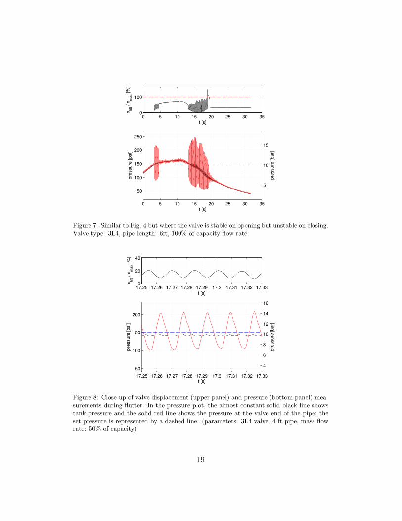
unstable on closing, see Fig. 6. Here note the initial oscillation, at around16 seconds, can be classified as flutter, using the scheme outlined in Sec. 1because the valve does not impact with its seat. There is a sudden transitionthough into chatter at around 19 seconds, at which point the oscillationsbecame strongly audible.

Figure 7 shows another intermediate case, where a flutter instability istriggered on opening the valve at around 3 seconds, which abruptly endsat 4.5 seconds. A similar instability is then triggered on closing the valve,which apart from a brief grazing event at around 15 seconds does not developinto chatter. Note that the final large excursion into large positive lift is ameasurement failure, as in Fig. 5 when the displacement transducer lostcontact with the valve as the valve closed.

Figure 8 shows a close-up of valve displacement and pressure fluctuationmeasured over several periods of steady, limit cycle oscillation during flutter.Zooming in on these pressure fluctuations, over this short time scale, weobserve that the pressure at the top of the pipe is one quarter of a cycleout of phase with that at the tank end. Moreover, the valve oscillation ishalf a cycle out of phase with the pressure. This data is typically of all the

17

0 5 10 15 20 25 30 350

20

40

t [s]

xlif

t / x

max [

%]

0 5 10 15 20 25 30 35

50

100

150

200

t [s]

pre

ssu

re [

psi]

4

6

8

10

12

14

16

pre

ssu

re [

ba

r]

Figure 6: Similar to Fig. 4 but showing a case where the valve is stable on opening butunstable on closing. Valve type: 3L4, pipe length: 4 ft, 50% of capacity flow rate.

oscillatory motion we have observed during flutter, and will prove importantin Section 4 where we seek an explanation for this phenomenon.

18

0 5 10 15 20 25 30 350

100

t [s]x

lift /

xm

ax [

%]

0 5 10 15 20 25 30 35

50

100

150

200

250

t [s]

pre

ssu

re [

psi]

5

10

15

pre

ssu

re [

ba

r]

Figure 7: Similar to Fig. 4 but where the valve is stable on opening but unstable on closing.Valve type: 3L4, pipe length: 6ft, 100% of capacity flow rate.

17.25 17.26 17.27 17.28 17.29 17.3 17.31 17.32 17.330

20

40

t [s]

xlif

t / x

max [

%]

17.25 17.26 17.27 17.28 17.29 17.3 17.31 17.32 17.33

50

100

150

200

t [s]

pre

ssu

re [

psi]

4

6

8

10

12

14

16

pre

ssu

re [

ba

r]

Figure 8: Close-up of valve displacement (upper panel) and pressure (bottom panel) mea-surements during flutter. In the pressure plot, the almost constant solid black line showstank pressure and the solid red line shows the pressure at the valve end of the pipe; theset pressure is represented by a dashed line. (parameters: 3L4 valve, 4 ft pipe, mass flowrate: 50% of capacity)

19

3.3. Comparison with simulations

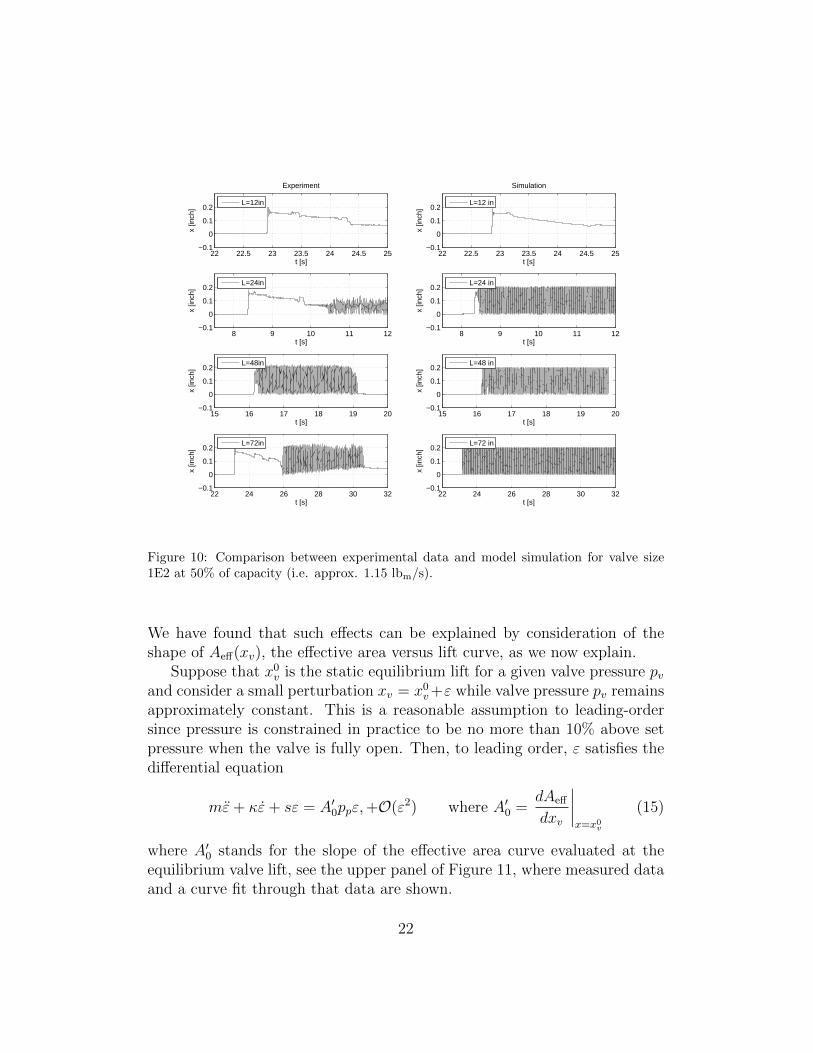
We have performed a large number of numerical computations, whichwill be analyzed later in detail. At this point we only emphasize that wehave been able to replicate all this behaviour using the simulation model asshown for example in Figure 9 and 10. In the simulations below, we used theeffective area curve depicted in the upper left panel of Figure 11.

5 10 15 20 25 30

0

0.2

0.4

Experiment

t [s]

x [in

ch]

L=12in

5 10 15 20 25 30

0

0.2

0.4

Simulation

t [s]

x [in

ch]

L=12 in

6 8 10 12 14

0

0.2

0.4

t [s]

x [in

ch]

L=24in

6 8 10 12 14

0

0.2

0.4

t [s]

x [in

ch]

L=24 in

5 10 15 20

0

0.2

0.4

t [s]

x [in

ch]

L=48in

5 10 15 20

0

0.2

0.4

t [s]

x [in

ch]

L=48 in

5 6 7 8 9 10 11 12

0

0.5

1

t [s]

x [in

ch]

L=72in

5 6 7 8 9 10 11 12

0

0.5

1

t [s]

x [in

ch]

L=72 in

Figure 9: Comparison between experimental data and model simulation for valve size 3L4at 50% of capacity (i.e. 6 lbm/s).

Figure 9 shows a comparison between experiment and simulation on arange of tests for the valve 3L4 with a mass flow rate 50% of the valve’scapacity rating, but for different pipe lengths. Note the strong qualitativeand good quantitative comparison between the two sets of data. Note alsothat this has been achieved without any parameter fitting, except for takinga reasonable, ballpark estimate of valve damping k. Nor have we botheredwith measuring and fitting an accurate effective area versus lift curve. This

20

figure also highlights the general trend we have seen in both the tests andsimulations; namely that for each value of mass flow rate, there is a criticalpipe length beyond which instability occurs. For pipes just longer than thiscritical length, the amplitude of the fluttering motion grows and transitionsinto chatter, becoming more violent with increasing pipe length.

We have experimented with changes to how the convective terms in theequations of motion are introduced, how much pipe friction was included,with the coefficient of damping and found that each of these had a weakeffect on the location of the critical pipe length at which instability occurred.The same is true of the shape of the effective area curve, although this didseem to change some of the transient dynamics close to the instability point,particular in whether instability was seen on opening, on closing or both.Changes to the coefficient of restitution obviously only affected the post-chattering motion and had no influence on the location of the instabilitypoint.

Figure 10 shows similar data for a much smaller valve, the 1E2. Thisvalve is designed to withstand much greater pressure build up. Again we seethe same trends in the data and the same level of correspondence betweenthe simulations and the test data, although we do note that the instabilitywhen it occurs appears more immediately and with larger amplitude in thesimulation than the data. Careful fitting of damping parameters and effectivearea curves would likely produce a stronger degree of quantitative similarity.

4. Identification of instability mechanisms

We shall now explore our experimental and computational findings inmore detail. In particular the mechanisms by which instabilities are triggeredwill be elucidated.

4.1. Valve jumps

The first issue we discuss is the possibility of a static instability (i.e.sudden jump in the valve lift without long-lasting oscillations). Such effectscan be seen on valve opening in the test data in Fig. 7 where there is a jumpup in valve lift on initial valve opening that triggers a flutter instabilityfollowed a second such jump that causes the instability to suddenly cease).Similar effects can also be observed on valve closing in the test and simulationdata in Fig. 9 where there are two jump downs, the second of which triggersa chatter type instability for a short time before the valve closes for good.

21

22 22.5 23 23.5 24 24.5 25−0.1

0

0.1

0.2

Experiment

t [s]

x [in

ch]

L=12in

22 22.5 23 23.5 24 24.5 25−0.1

0

0.1

0.2

Simulation

t [s]

x [in

ch]

L=12 in

8 9 10 11 12−0.1

0

0.1

0.2

t [s]

x [in

ch]

L=24in

8 9 10 11 12−0.1

0

0.1

0.2

t [s]

x [in

ch]

L=24 in

15 16 17 18 19 20−0.1

0

0.1

0.2

t [s]

x [in

ch]

L=48in

15 16 17 18 19 20−0.1

0

0.1

0.2

t [s]x

[inch

]

L=48 in

22 24 26 28 30 32−0.1

0

0.1

0.2

t [s]

x [in

ch]

L=72in

22 24 26 28 30 32−0.1

0

0.1

0.2

t [s]

x [in

ch]

L=72 in

Figure 10: Comparison between experimental data and model simulation for valve size1E2 at 50% of capacity (i.e. approx. 1.15 lbm/s).

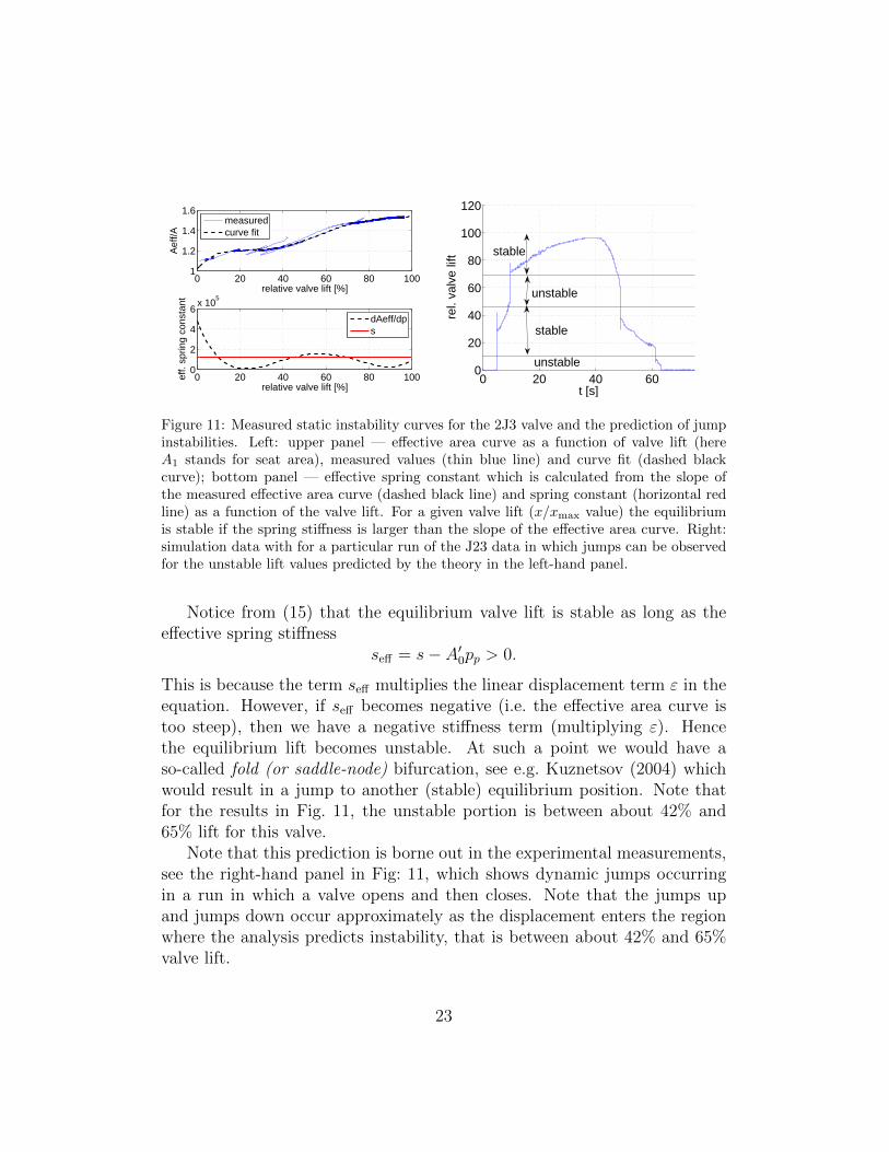
We have found that such effects can be explained by consideration of theshape of Aeff(xv), the effective area versus lift curve, as we now explain.

Suppose that x0v is the static equilibrium lift for a given valve pressure pv

and consider a small perturbation xv = x0v+ε while valve pressure pv remains

approximately constant. This is a reasonable assumption to leading-ordersince pressure is constrained in practice to be no more than 10% above setpressure when the valve is fully open. Then, to leading order, ε satisfies thedifferential equation

mε+ κε+ sε = A′0ppε,+O(ε2) where A′0 =dAeff

dxv

∣∣∣∣x=x0v

(15)

where A′0 stands for the slope of the effective area curve evaluated at theequilibrium valve lift, see the upper panel of Figure 11, where measured dataand a curve fit through that data are shown.

22

0 20 40 60 80 1001

1.2

1.4

1.6

relative valve lift [%]

Aef

f/A

measuredcurve fit

0 20 40 60 80 1000

2

4

6x 10

5

relative valve lift [%]

eff.

sprin

g co

nsta

nt

dAeff/dps

0 20 40 600

20

40

60

80

100

120

rel.

valv

e lif

t

t [s]

stable

unstable

stable

unstable

Figure 11: Measured static instability curves for the 2J3 valve and the prediction of jumpinstabilities. Left: upper panel — effective area curve as a function of valve lift (hereA1 stands for seat area), measured values (thin blue line) and curve fit (dashed blackcurve); bottom panel — effective spring constant which is calculated from the slope ofthe measured effective area curve (dashed black line) and spring constant (horizontal redline) as a function of the valve lift. For a given valve lift (x/xmax value) the equilibriumis stable if the spring stiffness is larger than the slope of the effective area curve. Right:simulation data with for a particular run of the J23 data in which jumps can be observedfor the unstable lift values predicted by the theory in the left-hand panel.

Notice from (15) that the equilibrium valve lift is stable as long as theeffective spring stiffness

seff = s− A′0pp > 0.

This is because the term seff multiplies the linear displacement term ε in theequation. However, if seff becomes negative (i.e. the effective area curve istoo steep), then we have a negative stiffness term (multiplying ε). Hencethe equilibrium lift becomes unstable. At such a point we would have aso-called fold (or saddle-node) bifurcation, see e.g. Kuznetsov (2004) whichwould result in a jump to another (stable) equilibrium position. Note thatfor the results in Fig. 11, the unstable portion is between about 42% and65% lift for this valve.

Note that this prediction is borne out in the experimental measurements,see the right-hand panel in Fig: 11, which shows dynamic jumps occurringin a run in which a valve opens and then closes. Note that the jumps upand jumps down occur approximately as the displacement enters the regionwhere the analysis predicts instability, that is between about 42% and 65%valve lift.

23

4.2. Flutter and chatter

The flutter instability bears all the hallmarks of a Hopf bifurcation, seee.g. Kuznetsov (2004). Such instabilities are characterized, upon quasi-staticparameter variation, by a transition to negative damping. In the so-calledsupercritical version of the bifurcation, a stable limit cycle motion ensues,whose amplitude grows like the square root of the distance of the parameterfrom its bifurcation point. The period of the limit cycle is related to theimaginary part (frequency) of the eigenvalue of the linearized system at theinstability point.

We have conducted a careful analysis of the valve motion and the pres-sure dynamics, notably extracted the frequency content of the experimentallymeasured valve displacement signals with the help of the fast Fourier trans-form (FFT). As shown in Table 2, once the valve goes unstable to flutter,the dominant frequencies obtained from both the displacement and pressuresignals are close to the pipe quarter-wave frequency, i.e. fqw = 4L/a with abeing the sonic velocity, and are a long way from the valve spring’s own res-onant frequency. Note that the measured dominant frequencies are slightlylower than the quarter-wave frequency, which is due to the inertial effects onthe end of the pipe as explained e.g. in Ih (1993).

This mode of instability is also consistent with the recordings shown inFig. 8 where we see the motion at the two ends of the pipe are a quarterof a cycle out of phase with each other. Although not presented here, the1E2 and the 3L4 valve measurements resulted in similar results. Hence weconclude that close to the critical pipe length, when the valve starts to flutter,the mode of vibration that is involved in the Hopf bifurcation is that whichcorresponds to a quarter standing wave in the pipe. Note that this is acoupled mode that involves both the fluid and the valve; see for exampleFig. 8 where the valve oscillates at the same frequency as the fluid pressure,albeit half a cycle out of phase as one would expect from physical principles.

This conclusion that the mode of instability at the Hopf bifurcation in-volves a quarter standing wave is confirmed by the simulations. Figure 12shows typical results for a pipe length just beyond that for which instabilityis triggered. This again confirms that the valve and the fluid are oscillating atthe same frequency, and the mode shape inside the pipe is clearly apparent.

4.3. Cycling and the 3% inlet pressure loss criterion

It is well known that over-sized valves are susceptible to cycling behaviour.Figures 13 and 14 show simulation results for the 3L4 valve at 6% of its

24

0 0.05 0.1 0.15 0.20

0.1

0.2

t [s]

x v [in

ch]

0 0.05 0.1 0.15 0.2100

200

300

400

t [s]p v [

psi g]

0 T/6 2T/6 3T/6 4T/6 5T/6 T0.025

0.03

0.035

x v [in

ch]

0 T/6 2T/6 3T/6 4T/6 5T/6 T260

270

280

p v [ps

i g]

0 0.5 1260

270

280

x [ft]

p [p

sig]

0 0.5 10

50

100

x [ft]

v [f

t/s]

0 200 400 600 800 10000

0.005

0.01

0.015

f [Hz]

ampl

. of

x v [in

ch]

0 200 400 600 800 10000

20

40

60

80

f [Hz]

ampl

. of

p v [ps

i g]

(a) (b)

(e) (f)

(g) (h)

(c) (d)

Figure 12: Simulated instability for 2J3 valve with L = 24 inch and 30% of capacity (i.e.close to the stability border). (a), (b) Time history of valve lift and pressure at valvejust after opening. (b),(c) Same information plot over one oscillation cycle. (d),(e) Modeshape of the fluid flow and pressure in the pipe over half a cycle. Different line types ineach plot represent the same time instant, which are plot at intervals of 1/8 of one periodof oscillation.

25

L [inch] mass flow rate[lb/s]

dominant freq.,experiment [Hz]

quarter-wavefrequency [Hz]

5.4 stable -24 9.2 stable -

13.2 stable -5.4 85.62 96.05

48 9.2 83.68 96.2313.2 83.37 95.985.4 62.34 64.13

72 9.2 61.98 6413.2 66.16 64.14

Table 2: Frequency content of the valve displacement signal (measurements) versus thecalculated pipe quarter-wave frequency (from the model) in the case of the 2J3 measure-ments. Note that the valve eigenfrequency is 45.6Hz.

maximum flow rate. In the first case, for a short pipe, the valve opens into astable regime. The pressure relief is such that too little fluid escapes duringthe initial valve opening that the pressure continues to build up again inthe tank. This then causes repeat openings, in a periodic very low frequencycycle. Such behaviour is not intended but is not likely to be damage inducing.

In contrast, Fig. 14 shows the same effect, but for a much longer pipe.Here when the valve opens, it is into a regime that is well into the instabilityregion, and chatter immediately ensues. Each time the valve opens there is aperiod of rapid chattering behaviour. This behaviour is likely to be damageinducing.

Cycling can also occur at higher flow rates, when the inlet piping pressureloss is too much. It has been recommended in the API standard RP520 thatthis pressure loss should be kept to under 3% of set pressure. The criticalpipe length corresponding to the ‘3% rule’ can easily be calculated, understandard assumptions about frictional losses of pipes of a given parameter.We briefly recall that the pressure loss due to wall friction in a straight pipeis given by (see Zucker and Biblarz (2002) for details)

∆p′ = λL

D

ρ

2v2 = λ

L

D

ρ

2

m2

ρ2A2, (16)

from which it is straightforward to find the critical pipe length L for which

26

0 2 4 6 8 100

50

100

perc

ent o

f ful

l lift

time [s]

0 2 4 6 8 10130

135

140

145

time [s]

p [p

si]

p

tankp

set

Figure 13: Simulation of cycling behaviour for the 3L4 valve with a 24 inch pipe at 6% ofits maximum mass flow rate.

27

0 2 4 6 8 100

50

100

perc

ent o

f ful

l lift

time [s]

0 2 4 6 8 1050

100

150

time [s]

p [p

si]

p

tankp

set

Figure 14: Similar to Figure 13 but for a 72 inch inlet pipe.

∆p′ = 0.03 × pset. Specifically, we used λ = 0.02 for Darcy friction factor,which is being four times larger than the Fanning friction factor (Zucker andBiblarz, 2002). This critical pipe length is plot on top of the stability mapsfor each of the pipes which we present in the following subsection.

4.4. Stability charts

Figures 15, 16 and 17 present a summary of the stability information wehave found for each of the three valves. The solid magenta curve in eachfigure shows the flutter boundary as computed using the simulation. Thiswas computed by visual inspection of the output of simulation runs eachmass flow rate at intervals of 0.1 lbm/s. A simple bisection method wasthen used to find the critical pipe length at which the Hopf bifurcation isobserved. This curve therefore represents the transition from stability (lowerpipe lengths) to instability (longer pipes).

28

0 0.5 1 1.5 2 2.5 30

12

24

36

48

60

72

84

mass flow rate [lbm

/s]

L [

in]

Stable (exp.) Unstable (exp.) Simulation

0 0.2 0.4 0.6 0.8 1 1.2

0

0.5

1

1.5

2

mass flow rate [kg/s]

L [

m]

3% pressure loss

Figure 15: Stability map for valve 1E2, see text for details.

On the same diagram we have plot the results of each of the experimentaltest runs, categorizing each run as either stable (marked with a red circle) orunstable (a red cross). In cases where different stability characteristics werefound upon valve opening and on closing, this is marked by both a circle anda cross.

Note the broad agreement between the location and the trend of theinstability curve between experiments and simulations. We should stresshere that there has been no parameter fitting whatsoever to achieve thisresult.

Superimposed on each stability chart is the 3% inlet pressure loss crite-rion derived from (16). Note how this curve has very little correlation withthe flutter instability boundary we have computed. This is hardly surprising,since this curve is supposed to represent a completely different effect, namelya threshold beyond which a valve may be susceptible to low frequency cy-cling, rather than the onset of a self-excited high-frequency Hopf bifurcationassociated with the quarter-wave mode in the pipe.

29

0 5 10 150

12

24

36

48

60

72

84

mass flow rate [lbm

/s]

L [

in]

Stable (exp.) Unstable (exp.) Simulation

0 1 2 3 4 5 6

0

0.5

1

1.5

2

mass flow rate [kg/s]

L [

m]

3% pressure loss

Figure 16: Similar to Fig. 15 but for valve 2J3.

5. Summary and outlook

In summary, we have produced a detailed, validated, fully parametrizedmathematical model of a direct spring operated pressure relief valve con-nected by a pipe to a tank. There is a good match between simulationoutputs from this model and detailed experimental measurements on threedifferent commercially available valves.

Within this model, we have found that the effects of line pressure lossare not important, although running the valve at low flow rates can resultin cycling in which the valve is prone to low-frequency oscillation with thevalve closed for a significant proportion of each period. Such instabilities arenot likely to be damage-inducing provided the valve opening itself is stable.

We have also found that the design of the valve can itself cause a formof static instability, in which the valves position jumps. These jumps canbe predicted by analyzing the new concept we have introduced here of theeffective-area versus lift curve. A simple criterion that compares the slopeof this curve to the valve stiffness can be used to predict these jump points.However, such instabilities do not lead to flutter or chatter behaviour, butcan contribute to cycling, or to rapid transitions between stable and unstable

30

0 2 4 6 8 10 12 14 160

12

24

36

48

60

72

84

mass flow rate [lbm

/s]

L [

in]

Stable (exp.) Unstable (exp.) Simulation

0 1 2 3 4 5 6 7

0

0.5

1

1.5

2

mass flow rate [kg/s]

L [

m]

3% pressure loss

Figure 17: Similar to Fig. 15 but for valve 3L4.

operation.Much more serious is a self-excited instability (a Hopf bifurcation) due

to a coupling between the valve and a pressure wave in the inlet pipe. Weshould stress that the observed instability is not in any sense due to resonantcoupling between the valve and the pipe’s natural frequency. Rather it is afully coupled mode of instability in which the valve in effect provides negativedamping to the lowest-frequency wave within the pipe, namely the quarterwave.

Moreover, we have been able to trace, both theoretically and in experi-ments, a critical curve in pipe-length vs. mass flow rate, beyond which theinstability occurs. This we can think of as a neutral stability curve. Beneaththis curve, the valve effectively provides damping to the acoustic pipe mode;whereas above it, we have the negative damping. Note the shape of theneutral stability curve is that for a pipe of a given length, the instability istriggered upon reducing the mass flow rate. For longer pipes (equivalently,lower mass flow-rates) the amplitude of the valve oscillations can becomeso-extreme that the valve first grazes with its seat. This leads to impactingmotion, or chatter. As first identified in Licsko et al. (2009), in terms of

31

dynamical systems theory, the transition to impacting motion is an exampleof a grazing bifurcation.

A much more delicate question is how the instability may be prevented inpractice. Any in-service pressure-relief event is in truth a transient operation,and there may be insufficient time at a given mass-flow rate in order to triggeran instability. In particular, the aim of any operation would be to be at a flowrate beyond the critical mass flow-rate for stability for the given inlet pipelength. This suggests that rapid opening of the valve to a sufficiently highflow rate, or rapid closing from a high flow rate to a low one may be one wayof avoiding instability in practice. Indeed, this was effectively observed inour experimental data, in which we found different thresholds for instabilitiesupon opening the valve than upon closing.

One thing to note from the study by Izuchi (2010) is that friction effectsfor very long pipes can have a stabilizing influence. We have found no directevidence for this effect in neither our test data nor simulations. However,it may be that we need to investigate much longer inlet pipes to observethis effect. However, in longer pipes, other pipe modes may additionallybecome relevant, as shown in Hayashi (1995) and Botros et al. (1997), whopredict further instabilities for longer pipes. This issue is worthy of furtherinvestigation.

We should stress that our conclusions on the mechanisms of instabilityare strictly speaking only valid for the particular valves tested in the particu-lar parameter region studied. Nevertheless, the mechanisms of instability wedescribe appear quite general, as evidenced by their occurrence for three sep-arate valves we have tested, and preliminary modeling studies that suggestthat they occur for a wide range of different parameter values. Moreover,our mathematical model approach is in principle easily extensible to capturefor example effects of back pressure, pilot-operated valves, and relief valvesin liquid. Each of these will be addressed in future work. Indeed, prelimi-nary analysis relevant to liquids (based on the study in Hos and Champneys(2012)) has revealed another mode of instability that involves the valve’sresonant frequency, without exciting quarter waves within the pipe.

Acknowledgements

This project was financially supported by Csaba Hos’s Bolyai fellowshipof the Hungarian Academy of Sciences.

32

References

Askari, E., Jeong, K.H., Amabili, M., 2013. Hydroelastic vibration of circularplates immersed in a liquid-filled container with free surface. Journal ofSound and Vibration .

Bazso, C., Champneys, A., Hos, C., 2013a. Bifurcation analysis of a simplifiedmodel or a pressure relief valve attached to a pipe. Submitted to SIAM J.Applied Dynamical Systems.

Bazso, C., Champneys, A., Hos, C., 2013b. Model reduction of a directspring-loaded pressure relief valve with upstream pipe. Submitted to IMAJ. Applied Math.

Bazso, C., Hos, C., 2013a. An experimental study on the stability of a directspring loaded poppet relief valve. Preprint.

Bazso, C., Hos, C., 2013b. On the static instability of liquid poppet valves.Submitted to Periodica Polytechnica Mechanical Engineering.

Bean, H., 1971. Report of ASME Research Committee on Fluids meters.Technical Report. ASME.

Beune, A., 2009. Analysis of high-pressure safety valves. Ph.D. thesis. PhDthesis. Eindhoven, The Netherlands: Eindhoven University of Technology.

Botros, K., Dunn, G., Hrycyk, J., 1997. Riser-relief valve dynamic interac-tions. Journal of Fluids Engineering 119, 671–679.

Cebeci, T., Shao, J.P., Kafyeke, F., Laurendeau, E., 2005. Computationalfluid dynamics for engineers: from panel to Navier-Stokes methods withcomputer programs. Springer.

Chabane, S., Plumejault, S., Pierrat, D., Couzinet, A., Bayart, M., 2009.Vibration and chattering of conventional safety relief valve under builtup back pressure, in: Proceedings of the 3rd IAHR International Meetingof the WorkGroup on Cavitation and Dynamic Problems in HydraulicMachinery and Systems, pp. 281–294.

D’Netto, W., Weaver, D., 1987. Divergence and limit cycle oscillations invalves operating at small openings. Journal of Fluids and Structures 1,3–18.

33

Francis, J., Betts, P., 1998. Backpressure in a high-lift compensated pres-sure relief valve subject to single phase compressible flow. Journal ofLoss Prevention in the Process Industries 11, 55 – 66. doi:10.1016/S0950-4230(98)00003-5.

Funk, J., 1964. Poppet valve stability. Journal of Basic Engineering 86, 207.

Green, W., Woods, G., 1973. Some causes of chatter in direct acting springloaded poppet valve, in: The 3rd International Fliud Power Symposium,Turin.

Habing, R., Peters, M., 2006. An experimental method for validating com-pressor valve vibration theory. Journal of Fluids and Structures 22, 683–697.

Hayashi, S., 1995. Instability of poppet valve circuit. JSME InternationalJournal. Ser. C, Dynamics, Control, Robotics, Design and Manufacturing38, 357–366.

Hayashi, S., Hayase, T., Kurahashi, T., 1997. Chaos in a hydraulic controlvalve. Journal of Fluids and Structures 11, 693 – 716.

Hos, C., Champneys, A., 2012. Grazing bifurcations and chatter in a pres-sure relief valve model. Physica D: Nonlinear Phenomena 241, 2068–2076.doi:10.1016/j.physd.2011.05.013.

Ih, J.G., 1993. On the inertial end correction of resonantors. Acustica 78,1–15.

Izuchi, H., 2010. Stability analysis of safety valve. American Institute ofChemical Engineers, 10th Topical Conference on Natural Gas UitilizationISBN: 9781617384417.

Kasai, K., 1968. On the stability of a poppet valve with an elastic support: 1st report, considering the effect of the inlet piping system. Bulletin ofJSME 11, 1068–1083.

Khalak, A., Williamson, C., 1997. Fluid forces and dynamics of a hydroe-lastic structure with very low mass and damping. Journal of Fluids andStructures 11, 973–982.

34

Kuznetsov, Y., 2004. Elements of applied bifurcation theory. Springer-Verlag.

Licsko, G., Champneys, A., Hos, C., 2009. Nonlinear analysis of a singlestage pressure relief valve. Int. J. Appl. Math 39, 12–26.

MacLeod, G., 1985. Safety valve dynamic Instability:An analysis of chatter.Journal of Pressure Vessel Technology 107, 172–177.

Madea, T., 1970a. Studies on the dynamic characteristic of a poppet valve:1st report, theoretical analysis. Bulletin of JSME 13, 281–289.

Madea, T., 1970b. Studies on the dynamic characteristics of a poppet valve:2nd report, experimental analysis. Bulletin of JSME 13, 290–297.

McCloy, D., McGuigan, R., 1964. Some static and dynamic characteristics ofpoppet valves, in: Proceedings of the Institution of Mechanical Engineers,Prof Eng Publishing. pp. 199–213.

Misra, A., Behdinan, K., Cleghorn, W., 2002. Self-excited vibration of acontrol valve due to fluid-structure interaction. Journal of Fluids andStructures 16, 649 – 665.

Moussou, P., Gibert, R., Brasseur, G., Teygeman, C., Ferrari, J., Rit, J.,2010. Instability of pressure relief valves in water pipes. Journal of PressureVessel Technology 132.

Nayfeh, A., Bouguerra, H., 1990. Non-linear response of a fluid valve. Inter-national Journal of Non-Linear Mechanics 25, 433–449.

Song, X.G., Park, Y.C., Park, J.H., 2011. Blowdown prediction of a conven-tional pressure relief valve with a simplified dynamic model. Mathematicaland Computer Modelling 57, 279–288.

Thomann, H., 1976. Oscillations of a simple valve connected to a pipe.Zeitschrift f ur Angewandte Mathematik und Physik (ZAMP) 27, 23–40.

Vaughan, N., Johnston, D., Edge, K., 1992. Numerical simulation of fluid flowin poppet valves. Proceedings of the Institution of Mechanical Engineers206, 119–127.

35

Warren, M., 1983. Appropriate boundary conditions for the solution ofthe equations of unsteady one-dimensional gas flow by the Lax-Wendroffmethod. International Journal of Heat and Fluid Flow 4, 53–59.

Ye, Q., Chen, J., 2009. Dynamic analysis of a pilot-operated two-stagesolenoid valve used in pneumatic system. Simulation Modelling Practiceand Theory 17, 794–816.

Zucker, D., Biblarz, O., 2002. Fundamentals of Gas Dynamics. New York:John Wiley and Sons.

Zucrow, M.J., Hoffman, J.D., 1976. Gas dynamics. volume 1. New York:John Wiley and Sons, 1976.

Zung, P., Perng, M., 2002. Nonlinear dynamic model of a two-stage pressurerelief valve for designers. Journal of dynamic systems, measurement, andcontrol 124, 62–66.

36