Dynamic Asset Allocation with Stochastic Income and ... - Dynamic Asset... · Dynamic Asset...
66
Dynamic Asset Allocation with Stochastic Income and Interest Rates ∗ February 28, 2005 Claus Munk † Carsten Sørensen Dept. of Accounting and Finance Department of Finance University of Southern Denmark Copenhagen Business School E-mail: [email protected] E-mail: [email protected] * This research is financially supported by INQUIRE EUROPE. We appreciate comments from par- ticipants at presentations at the EIASM Workshop on Dynamic Strategies in Asset Allocation and Risk Management in Brussels and at the Goethe University in Frankfurt. † Corresponding author. Full address: Department of Accounting and Finance, University of Southern Denmark, Campusvej 55, DK-5230 Odense M, Denmark. Phone: +45 6550 3257. Fax: +45 6593 0726.
Transcript of Dynamic Asset Allocation with Stochastic Income and ... - Dynamic Asset... · Dynamic Asset...
Dynamic Asset Allocation with Stochastic
Income and Interest Rates∗
February 28, 2005
Claus Munk† Carsten Sørensen
Dept. of Accounting and Finance Department of Finance
University of Southern Denmark Copenhagen Business School
E-mail: [email protected] E-mail: [email protected]
∗This research is financially supported by INQUIRE EUROPE. We appreciate comments from par-
ticipants at presentations at the EIASM Workshop on Dynamic Strategies in Asset Allocation and Risk
Management in Brussels and at the Goethe University in Frankfurt.
†Corresponding author. Full address: Department of Accounting and Finance, University of Southern
Denmark, Campusvej 55, DK-5230 Odense M, Denmark. Phone: +45 6550 3257. Fax: +45 6593 0726.

Dynamic Asset Allocation with Stochastic
Income and Interest Rates
February 28, 2005
Abstract. We investigate the optimal investment and consumption
choice of individual investors with uncertain future labor income operat-
ing in a financial market with stochastic interest rates. Since the present
value of the individual’s future income is a main determinant of the opti-
mal behavior and this present value depends heavily on the interest rate
dynamics, the joint stochastics of income and interest rates will have con-
sequences beyond the separate effects of stochastic income and stochastic
interest rates. We study both the case where income risk is spanned and
there are no portfolio constraints and the case with non-spanned income
risk and a constraint ruling out borrowing against future income. For the
spanned, unconstrained problem we study a special case in which we ob-
tain closed-form expressions for the optimal policies. For the unspanned,
constrained problem we implement a numerical solution technique and
compare the solutions to the spanned, unconstrained problem. We also
allow for typical life-cycle variations in labor income.
Keywords. Portfolio management, labor income risk, interest rate risk,
hedging, borrowing constraints, life-cycle
Dynamic Asset Allocation with Stochastic Income and
Interest Rates
1 Introduction
The household participation in financial markets creates a demand and a need for compe-
tent investment advice. The optimal investment strategy for a given individual will depend
both on market characteristics, such as the dynamics of asset prices and interest rates, and
on personal characteristics, such as risk aversion, time preference, and labor income. In this
paper we will study the optimal strategies when both interest rates and the labor income
rate of the individual are stochastic. Stochastic interest rates is the main source of shifts in
the investment opportunity set, and the effect of interest rate uncertainty on the optimal
strategies of an investor without labor income is by now relatively well-studied in the liter-
ature. There are also a number of studies of the effects of labor income uncertainty on the
optimal strategies, but they all assume constant investment opportunities. (References are
given below.) We argue and demonstrate in this paper that allowing jointly for stochastic
interest rates and labor income will affect the optimal investment strategy beyond the sep-
arate effects of stochastic income and stochastic interest rates. In addition, the expected
income rate in the near future is likely to depend on the interest rate level, which serves as
a good proxy of the overall well-being of the economy. High interest rates typically reflect
high growth rates of the economy which may lead to an upward pressure on wages, higher
bonuses, fewer lay-offs, etc.
We first set up a quite general model of the financial market in which the interest rate
dynamics is given by a one-factor model and several risky assets (bonds and stocks) are
traded. The consumer-investor is assumed to have a time-additive utility for consumption
exhibiting constant relative risk aversion and a risky labor income stream, which is correlated
with both the interest rate and the risky asset prices. We calibrate the model to actual data
on income and financial returns.
For the special case of the model, where the income risk can be fully hedged by appro-
priate financial investments and there are no portfolio constraints, we are able to obtain
closed-form expressions for the value of the labor income stream (i.e. human wealth) and
the optimal consumption and investment strategies, which allows us to perform a detailed
analysis. While it is well-known from the literature that the labor income increases the
optimal speculative investments due to a wealth effect, we show that the relative allocation
to bonds and stocks can be significantly affected by the presence of uncertain labor income
1

for several reasons. First, bonds and stocks can be differently correlated with labor income
shocks so that bonds may be better for hedging income rate shocks than stocks or vice
versa. Second, risk-averse investors want to hedge total wealth against shifts in investment
opportunities. When the short-term interest rate captures the investment opportunities,
the appropriate asset for this hedging motive is the bond. Third, since human wealth is
defined as the discounted value of the future income stream, it will in general be sensitive
to the interest rate level like a bond and, hence, the income stream represents an implicit
investment in a bond, so that the explicit bond investment is reduced. As explained above,
the expected growth of labor income may itself be sensitive to the level of interest rates,
which will also affect hedging demand. We also give a detailed numerical analysis of this
special case, illustrating the sign and magnitudes of various portfolio components and their
sensitivity to key parameters. The optimal strategies will often involve extremely large posi-
tions in bonds and stocks and an extreme level of borrowing. In this unconstrained case, the
investor is even allowed to borrow against future labor income so that his financial wealth
in some situations will be negative.
The assumptions of spanned income and no portfolio constraints are certainly question-
able. It is generally believed that labor income risk is not fully insurable and, due to moral
hazard and adverse selection considerations, investors can only to a very limited extent bor-
row money using future income as implicit collateral. Introducing non-spanned income risk
and portfolio constraints, we must solve the utility-maximization problem by a numerical
method. We solve the dynamic programming equation associated with the problem with
a finite difference technique. We show in numerical examples that imposing the constraint
that financial wealth has to stay non-negative at all times reduces risk-taking considerably
but will still involve a high degree of borrowing and large positions in the bond and stock.
When we, in addition, prevent the individual from taking short positions (and hence from
borrowing at all), we see that the optimal portfolio will often consist of 100% in the stock,
but this result is sensitive to correlation parameters, the degree of risk aversion, and the
investment horizon.
Let us briefly review the relevant literature for this study. As first noted by Merton
(1971), long-term investors will generally hedge stochastic variations in the investment op-
portunity set, e.g. interest rates, excess returns, and volatilities. Several recent papers study
optimal investments in concrete settings with interest rate uncertainty. Sørensen (1999) and
Brennan and Xia (2000) consider interest rate dynamics as in the Vasicek (1977) model
and assume complete financial markets and constant market prices of both interest rate risk
and stock market risk. They find that the optimal investment strategy of an investor with
power utility of terminal wealth only is a simple combination of the mean-variance optimal
portfolio, i.e. the optimal portfolio assuming investment opportunities do not change, and
2

the zero-coupon bond maturing at the end of the investment horizon. Liu (1999) provides
similar insight using the one-factor square-root model of Cox, Ingersoll and Ross (1985).
Furthermore, Liu shows that in a complete and “affine” market the appropriate interest
rate hedge instrument for an investor with a time-additive power utility of consumption is
some sort of coupon bond rather than a zero-coupon bond. Other studies of portfolio choice
with uncertain interest rates include Brennan, Schwartz, and Lagnado (1997), Campbell and
Viceira (2001), Detemple, Garcia, and Rindisbacher (2003), and Munk and Sørensen (2004).
None of these papers take into account a labor income stream of the investor, although labor
income is the main source of funds for most individuals.
On the other hand, several papers discuss how the presence of a labor income process af-
fects the consumption and investment decisions of individual investors, but all in the context
of constant financial investment opportunities. A deterministic income stream is equivalent
to an implicit investment in the riskless asset and, hence, it is optimal to invest a higher
fraction of financial wealth in the risky assets than in the no-income case; cf., e.g., Hakans-
son (1970) and Merton (1971). With stochastic income, but fully hedgeable income risk,
the optimal unconstrained strategies can be deduced from the optimal strategies without
labor income; see, e.g., Bodie, Merton, and Samuelson (1992). Duffie, Fleming, Soner, and
Zariphopoulou (1997), Koo (1998), and Munk (2000) study (mostly by use of numerical
methods) the valuation of income and the optimal consumption and investment strategies
of an infinite-horizon, liquidity constrained power utility investor with non-spanned income
risk. The presence of liquidity constraints can significantly decrease the individual’s im-
plicit valuation of the future income stream and, hence, dampen the quantitative effects of
income on portfolio choice. Other recent papers on consumption and portfolio choice with
stochastic income include Cocco, Gomes, and Maenhout (2005), Constantinides, Donaldson,
and Mehra (2002), El Karoui and Jeanblanc-Picque (1998), He and Pages (1993), Heaton
and Lucas (1997), and Viceira (2001). Besides working with constant investment oppor-
tunities, the concrete models with stochastic income in these papers assume a single risky
asset, interpreted as the stock market index. Since different risky assets will have different
correlations with the labor income of a given individual, this assumption is not without loss
of generality. In our numerical examples, we will have two risky assets, namely a stock and
a bond.
The outline of the rest of the paper is as follows. In Section 2 we set up the general
model of the financial market and specify the preferences and income of the individual.
Section 3 discusses the calibration of the model and the choice of benchmark parameter
values. Section 4 focuses on the case with spanned income uncertainty and unconstrained
investment strategies, where we derive, illustrate, and discuss the explicit solution to the
decision problem of an investor with constant relative risk aversion. In Section 5 we then turn
3
to the case with unspanned income uncertainty and liquidity constraints on the investment
strategy, where again we provide relevant numerical examples. In Section 6 we study the
effects of introducing a realistic life-cycle pattern in expected income growth. Section 7 gives
some concluding remarks. The appendices contain proofs of propositions and lemmas and
also a detailed description of the numerical method applied in the solution of the problem
with unspanned income and liquidity constraints.
2 Description of the model
We model the intertemporal consumption and investment choice of a price-taking indi-
vidual who can trade in stocks and bonds and receives a stochastic stream of income from
non-financial sources, say labor income. We assume that the economy has a single perishable
consumption good which serves as a numeraire so that all asset prices, interest rates, and
income rates are specified in units of this good, i.e. in real terms.
2.1 Financial assets
We assume that the real short-term interest rate follows the Vasicek (1977) model,
drt = κ (r − rt) dt− σr dzrt, (1)
where κ, r, and σr are positive constants, and zr = (zrt)t≥0 is a standard Brownian motion.
We also assume that the market prices of interest rate risk, λr, is constant. The price of a
zero-coupon bond paying one unit of account at some time T is then given by
BTt ≡ BT (rt, t) = e−a(T−t)−b(T−t)rt , (2)
where
b(τ) =1
κ
(
1 − e−κτ)
, (3)
a(τ) = y∞[τ − b(τ)] +σ2
r
4κb(τ)2, (4)
y∞ = r +σrλr
κ− σ2
r
2κ2. (5)
Here y∞ is the limit of the yield of a zero-coupon bond as maturity goes to infinity, i.e. the
asymptotic long rate.
Any desired interest rate exposure can be obtained by combining deposits/loans at the
short-term interest rate (interpreted as cash or the bank account) and a single default-free
4
real bond.1 The dynamics of the price Bt of such a bond is given by
dBt = Bt [(rt + σB(rt, t)λr) dt+ σB(rt, t) dzrt] , (6)
where σB(rt, t) > 0 is the bond price volatility, which will generally depend on both the
interest rate level and the time-to-maturity and hence on time. However, for a zero-coupon
bond the volatility is σrb(T − t), which depends on the time-to-maturity T − t, but not on
the interest rate level. The bond price has a perfectly negative (instantaneous) correlation
with the interest rate, ρBr = −1.
In addition to the bond, we assume that agents can invest in stocks. In the general
analysis we will allow agents to trade in n stocks. The price of stock i at time t is denoted
by Sit and is assumed to evolve as
dSit = Sit
(rt + ψi) dt+ σi
ρiB dzrt +
i∑
j=1
kij dzjt
, i = 1, . . . , n, (7)
where zSt = (z1t, . . . , znt)⊤ is an n-dimensional standard Brownian motion independent of
zrt, ψi is the constant expected excess return, σi is the constant volatility, and ρiB = −ρir
is the constant correlation between stock i and the bond. Finally, the constants kij will
determine the correlations between the n stocks.2 We gather the dynamics of stock prices
in vector form as
dSt = diag(St) [(rt1n + ψ) dt+ diag(σS) ρSB dzrt +K dzSt] , (8)
where diag(x) means the diagonal matrix with the vector x along the diagonal, 1n is an
n-dimensional vector of ones, K is the lower triangular matrix [kij ], and we have introduced
the vectors ψ = (ψ1, . . . , ψn)⊤, σS = (σ1, . . . , σn)⊤, and ρSB = (ρ1B , . . . , ρnB)⊤
. Note that
in order to focus on the effects of combining stochastic labor income and stochastic interest
rates, we have chosen to assume constant expected excess returns and volatilities on the
stocks, despite ample evidence that these quantities vary over the business cycle.
To simplify some of the following expressions, we introduce the vector Pt = (Bt, St)⊤ of
prices of all n+ 1 risky assets. By combining the dynamics of Bt and St, we get
dPt = diag(Pt) [(rt1n+1 + Σ(rt, t)λ) dt+ Σ(rt, t) dzt] , (9)
1We assume that real, i.e. inflation-indexed, bonds are traded. Brennan and Xia (2002) and Munk,
Sørensen, and Vinther (2004) study how real interest rate risk affects optimal investments when the traded
bonds are nominal.
2The correlation between stock i and stock l (with i ≤ l) is ρil = ρiBρlB +∑i
j=1kijklj . Since ρ11 = 1, we
must have k11 =√
1 − ρ21B
. We have ρ12 = ρ1Bρ2B+k11k21 implying that k21 = (ρ12−ρ1Bρ2B)/√
1 − ρ21B
.
Since 1 = ρ22 = ρ22B
+ k2
21+ k2
22, we can then conclude that k22 =
√
1 − ρ22B
− k2
21. Continuing this way,
we can express all the kij constants in terms of the correlations between the individual stocks and the
correlations between the stocks and the bond.
5

where z = (zr, zS)⊤ and Σ(rt, t) is the (n+ 1) × (n+ 1) matrix
Σ(rt, t) =
σB(rt, t) 0
diag(σS)ρSB diag(σS)K
.
Furthermore, λ = (λr, λS)⊤ where λS = (λ1, . . . , λn)⊤ is the n-dimensional vector
λS = K−1[
diag(σS)−1ψ − ρSBλr
]
.
The vector λ has the interpretation as the market price of risk vector. For example, λi is
the excess expected return per unit volatility on an asset which is only sensitive to zi and
not to any other random shocks.
2.2 The preferences and labor income of the individual
We assume throughout the paper that the individual has a time-additive utility function
of consumption ct and possibly terminal wealth WT and seeks to maximize
E
[
∫ T
0
e−δtU(ct) dt+ εe−δTU(WT )
]
,
where T is the time of death, assumed non-random, and ε is a 0-1 parameter indicating
whether or not the individual has utility from leaving wealth to her heirs. Throughout the
paper we use a power utility function
U(c) =1
1 − γc1−γ ,
where γ > 0 is the constant relative risk aversion.
We set up a relatively simple model of income that is tractable and allows us to focus on
the interaction between stochastic income and stochastic interest rates. We assume that the
individual receives a continuous stream of non-negative income from non-financial sources
throughout her life. The income rate at time t is denoted by yt. We assume that yt evolves
as3
dyt = yt
[
(ξ0(t) + ξ1rt) dt+ σy(t)
ρ⊤
yP dzt +√
1 − ‖ρyP ‖2 dzyt
]
, (10)
where zy = (zyt) is a one-dimensional standard Brownian motion independent of zr and zS .
The constant vector ρyP is defined as (ρyB , ρyS)⊤, where ρyB = −ρyr is the instantaneous
correlation between the income rate and the bond price, and the vector ρyS is given by
ρyS = K−1 (ρyS − ρSBρyB), where ρyS is the vector of correlations between the income rate
and the stocks and the other terms have been defined above. If ‖ρyP ‖2 = 1, the income rate
3As most authors, we have modeled the income stream as an exogenously given process. Of course, in
real life the individual can affect her labor income to some extent by choice of education and effort. To avoid
further complications of the model we do not endogenize the labor supply decision. We refer the reader to
Bodie, Merton, and Samuelson (1992) and Chan and Viceira (2000).
6
is spanned, i.e. only sensitive to the traded risks represented by z. If that is the case, and
there are no portfolio constraints, the income process can be replicated by some dynamic
trading strategy of the traded assets and hence valued as a traded asset.
The income process have the following features:
• The percentage drift ξ0(t) + ξ1rt and volatility σy(t) are allowed to depend on time
in order to reflect the empirically relevant variations in expected income growth and
uncertainty over the life of an individual, cf. e.g. Hubbard, Skinner, and Zeldes (1995)
and Cocco, Gomes, and Maenhout (2005).
• In contrast to other studies, we allow the drift to depend on the interest rate in order to
incorporate the plausible link between the expected growth in income and the overall
well-being of the economy.
• For simplicity, we ignore retirement and assume that y describes the income rate until
time T .
• Our model does not allow for jumps in income, although jumps reflecting for example
lay-offs may be relevant. Results of Cocco, Gomes, and Maenhout (2005) indicate that
even a small probability of a large sudden income reduction may substantially affect
portfolio choice. However, for many individuals the possible unemployment periods
are likely to be rather short and in many countries individuals can partly insure against
temporary income losses due to unemployment. Hence, it may not be that important
to explicitly allow for large drops in income.
• Several empirical studies suggest a link between expected excess stock returns and
the expected growth and riskiness of labor income (see for example Jagannathan and
Wang (1996), Julliard (2004), and Storesletten, Telmer, and Yaron (2004)), but we
will not address the potential implications for portfolio choice in this paper.
2.3 Optimal strategies
The individual is to choose a consumption strategy c = (ct) and an investment strategy
θ = (θt). Here ct is the rate at which goods are consumed at time t with the natural
requirement that ct ≥ 0 at all times and in all states of the economy. Furthermore, θt is
a vector (θBt, θSt)⊤ of the amounts (i.e. units of the consumption good) invested at time t
in the bond and the n stocks. With Wt denoting the financial wealth of the investor at
time t, the amount invested in the bank account (held in “cash”) is residually determined
as θ0t = Wt − θBt − θ⊤
St1n. Given a consumption strategy c and an investment strategy θ,
the financial wealth of the individual Wt evolves as
dWt = (rtWt + θ⊤
t Σ(rt, t)λ− ct + yt) dt+ θ⊤
t Σ(rt, t) dzt. (11)
7

The consumption and investment strategies must satisfy some technical conditions for the
wealth process to be well-defined. If there are no other restrictions on the strategies (except
ct ≥ 0) we denote by Aunct the set of admissible consumption and investment strategies (c, θ)
over the time interval [t, T ]. We will also consider the case where it is not possible for the
individual to borrow funds using future income as collateral so that her financial wealth Wt
must stay non-negative at all times and in all states of the world.4 In a continuous-time
setting this is implemented by requiring that whenever the financial wealth hits zero, the
investor must eliminate her positions in bonds and stocks. After she have received labor
income, she may again enter the markets for risky securities. We denote the set of admissible
strategies with this constraint by Acont .
The indirect utility function of the individual is defined as
J(W, r, y, t) = sup(c,θ)∈At
Et
[
∫ T
t
e−δ(s−t)U(cs) ds+ εe−δ(T−t)U(WT )
]
, (12)
where the expectation is computed given the values of W, r, y at time t and given the strategy
(c, θ). The set At is either equal to Aunct or Acon
t . With the assumed CRRA utility function
the marginal utility is infinite at zero consumption so that the non-negativity constraint on
consumption is not binding. The Hamilton-Jacobi-Bellman (HJB) equation associated with
this dynamic optimization problem is
δJ = supc,θ
U(c) + Jt + JW (rW + θ⊤Σλ− c+ y) +1
2JWW θ⊤ΣΣ⊤θ
+ Jrκ[r − r] +1
2Jrrσ
2r + Jyy(ξ0 + ξ1r) +
1
2Jyyy
2σ2y
− JWrθ⊤Σe1σr + JWyyσyθ
⊤ΣρyP + Jryyρyrσyσr
,
(13)
where e1 = (1,0n)⊤, subscripts on J denote partial derivatives, and we have suppressed the
arguments of the functions for notational simplicity. The terminal condition is J(W, r, y, T ) =
εU(W ) = εW 1−γ/(1 − γ).
The first-order condition for consumption is the standard envelope condition
U ′(ct) = JW (Wt, rt, yt, t) ⇒ ct = [JW (Wt, rt, yt, t)]−1/γ
. (14)
For the unrestricted investment case the first-order condition for the portfolio θ implies that
θt = − JW
JWW(Σ(rt, t)
⊤)−1λ− JWy
JWWyσy(t) (Σ(rt, t)
⊤)−1ρyP +
JWr
JWW
σr
σB(rt, t)e1. (15)
The first part corresponds to the standard mean-variance optimal portfolio, the second part
is a hedge against changes in the income rate, while the third part is a hedge against changes
4This “hard” borrowing constraint is standard in the literature. A recent paper by Davis, Kubler, and
Willen (2003) studies the portfolio choice under a “soft” borrowing constraint that allows individuals to
borrow even with a negative current wealth although at a rate higher than the riskless interest rate. Their
study assumes constant interest rates. To focus on the interaction between stochastic interest rates and
stochastic labor income we stick to the “hard” borrowing constraint, which is easier to handle.
8

in the interest rate. The income hedge term reflects a position in the portfolio with relative
weights given by (Σ(rt, t)⊤)
−1ρyP /1
⊤
n+1 (Σ(rt, t)⊤)
−1ρyP . This is the portfolio with the
maximal absolute correlation with the income rate of the individual, cf. Ingersoll (1987,
Ch. 13). This maximal correlation equals ‖ρyP ‖ so if the income rate is spanned, this
correlation will equal 1. Since the bond price is perfectly negatively correlated with the
interest rate, the interest rate is hedged by a position in the bond only. In contrast, the
income hedge and the mean-variance terms generally involve all risky assets. The remaining
wealth, Wt − θ⊤
t 1n+1, is invested in the bank account. In Section 4 we consider the case
where the income rate is spanned, which – given our other assumptions – allows the optimal
strategies to be computed in closed form.
3 Calibration of parameters
In the calibration of income parameters, we apply modeling ideas from the discrete-
time settings of Cocco, Gomes, and Maenhout (2005) and Campbell and Viceira (2002) and
decompose log-income into a personal component and a common component, so that the
income of individuals with characteristics i is given by
log yit = P i(t) + log yc
t (16)
where the personal component P i(t) reflects the expected life-cycle income of individuals
with characteristics i. The dynamics of the common income component are described by an
income process of the form in (10), but with constant parameters, ξ0(t) = ξ0 and σy(t) = σy.
In order to adopt estimation results from Cocco, Gomes, and Maenhout (2005) and
Campbell and Viceira (2002), we will in our calibration approach assume that the personal
income component P i(t) is deterministic and described by a third-order polynomial in time
(age),
P i(t) = ai + bit+ cit2 + dit3
where ai, bi, ci, and di are constant parameters. The polynomial form of P i(t) only applies
for age 20 until 65 (years). In the discrete-time framework of Cocco, Gomes, and Maen-
hout (2005), it is thus assumed that the retirement income level for age 66 and higher is
proportional to the income level at age 65 with a replacement rate, P i. We will adopt this
form, and in our continuous-time setting we simply linearly interpolate the income level
in the one-year period between age 65 and age 66. Cocco, Gomes, and Maenhout (2005)
use Panel Study on Income Dynamics (PSID) data to estimate labor income as a function
of age and other characteristics. In our numerical analysis of life-cycle allocations, we will
adopt their estimated third-order polynomial structures and replacement rates for groups
characterized by three different educational backgrounds: “No High school”, “High school”,
and “College”. The polynomial life-cycle income profiles are illustrated in Figure 1, and the
9
polynomial coefficients used in the figure are reproduced from Cocco, Gomes, and Maenhout
(2005) in Table 1.
[Figure 1 about here.]
[Table 1 about here.]
With the above decomposition and assumptions, it can be inferred (by an application of
Ito’s lemma) that the individual income process is of the form in (10) with,
ξ0(t) = ξ0 +dP i(t)
dt= ξ0 +
bi + 2cit+ 3dit2 if 20 ≤ t ≤ 65
−(1 − P i) if 65 < t < 66
0 if t ≥ 66
(17)
We take the income rate volatility to be σy(t) = 0.10 for t ≤ 65 and σy(t) = 0 for t ≥ 65.
In order to estimate parameters of the common component of labor income as well as
correlations and parameters of real interest rates and stock prices, we consider the case with
only a single stock. The relevant dynamics are described by the real interest rate dynamics
in (1), the single-stock special case of (8), and an income process of the form in (10) with
ξt(t) = ξ0 and constant income volatility σy. Let Yt = (log yct , logSt, rt)
′, then the relevant
dynamics can be summarized by the linear stochastic differential equation,
dYt = (A+BYt)dt+ V dzt (18)
where
A =
ξ0 − 12σ
2y
ψ − 12σ
2S
κr
, B =
0 0 ξ1
0 0 1
0 0 −κ
, V V ′ =
σ2y ρySσyσS ρyrσyσr
ρySσyσS σ2S ρSrσSσr
ρyrσyσr ρSrσSσr σ2r
,
and zt is a three-dimensional standard Brownian motion. The discrete-time solution to the
linear stochastic differential equation in (18) is a discrete-time VAR(1)-model of the form
Yt+∆ = A(Ψ,∆) +B(Ψ,∆)Yt + ǫt+∆, ǫt+∆ ∼ N(0,Ω(Ψ,∆)) (19)
where Ψ = (ξ0, ξ1, ψ, κ, r, σy, σS , σr, ρyS , ρyr, ρSr) denotes the set of parameters to be esti-
mated. The functions A(Ψ,∆), B(Ψ,∆), and Ω(Ψ,∆) can be obtained in closed-form using
the general solution formula for linear stochastic differential equations (see, e.g., Karatzas
and Shreve (1988, pp. 354-357)).
The VAR(1)-model in (19) is estimated by maximum likelihood using quarterly US data
which span the period from 1951 until 2003.5 The total number of observation time points is
5The numerical maximum likelihood estimation is carried out using the software program GAUSS. How-
ever, in evaluating the relevant first and second order moments we used the analytical evaluation tools in
the software program Mathematica and pasted the relevant analytical results into the GAUSS program.
10

208. The per capital income data was obtained from the Personal Income and Its Disposition
NIPA table of the National Economic Accounts. The income data is the per capita disposable
personal income after personal current taxes and subtracted personal income from financial
assets. The cum dividend stock returns are constructed using quarter-end values of the S&P
500 index over the period while the S&P 500 dividends and the CPI-index data are adopted
from Shiller (2000); the updated data were downloaded from Robert Shiller’s homepage. All
income and stock prices are in real terms (using the CPI-index as deflator). Real interest
rates are constructed by subtracting an estimate of the inflation rate from the 3-month
nominal interest rate. The subtracted inflation rate is obtained as the average realized
inflation rate in the last four quarters relative to the same quarters one year earlier. The
applied data is illustrated in Figure 1 where the income index and the stock index are scaled
so that they start out in one in 1951 (and zero for the logarithmic value).
[Figure 2 about here.]
The estimated parameters values are displayed in Table 2 together with our chosen
benchmark parameters for the subsequent numerical analysis. Our benchmark parameters
are chosen close to the estimated values (in most cases the benchmark parameters are just
rounded off). Some parameters are chosen to be similar or comparable to those applied by,
e.g., Campbell and Viceira (2002) who use ψ = 4% and a real interest rate level of 2%. The
volatility in the per capita log-income process is estimated at 2.08%, but our benchmark
parameter value is set significantly higher at 10%. This choice is motivated by results based
on household level data that indicate that individual income volatility is at least at this
level.6
Individual income may be more or less correlated with basic macro economic values such
as real interest rates and stock returns, but we choose correlations close to the estimated
values for per capita income as our benchmark parameter values. Other authors have pre-
viously estimated correlations between labor income and stock market returns. Davis and
Willen (2000) find that – depending on the individuals sex, age, and educational level –
the correlation between aggregate stock market returns and labor income shocks is between
-0.25 and 0.3, while the correlation between industry-specific stock returns and labor income
shocks is between -0.4 and 0.1. Campbell and Viceira (2002) report that the correlation be-
tween aggregate stock market returns and labor income shocks is between 0.328 and 0.516.
Heaton and Lucas (2000) find that the labor income of entrepreneurs typically is more highly
correlated with the overall stock market (0.14) than with the labor income of ordinary wage
6For example, the estimates presented in Cocco, Gomes, and Maenhout (2005) and Campbell and Viceira
(2002), among others, suggest a permanent income volatility slightly above 10% (for all three educational
groups) as well as transitory income volatility components of the magnitude 25%. Our model of income
dynamics include basically only shocks of the permanent type.
11
earners (-0.07). In all our numerical experiments we will assume that individuals invest in
only one stock, representing the stock market index. While a broad stock market index is
clearly less than perfectly correlated with individual labor income, it is to be expected that
a larger fraction of the income rate variations can be hedged using multiple risky assets,
but we have no information about the typical correlations between a labor income stream
and individual stocks–and hence we really do not know how large a fraction of the risk of a
typical labor income stream that can be hedged in the financial markets.7
Our estimation approach does not involve the risk premium on real interest rate risk, but
our benchmark parameter value is set to λr = 0. This value is not far from the about 1%
historical excess return on longer-term nominal bonds which is usually reported in empirical
studies; see, e.g., Dimson, Marsh, and Staunton (2002). The long-term yield is then 1.92%,
the yield curve is increasing if the current short rate is below 1.88%, decreasing if the current
short rate exceeds 2%, and humped for intermediary values. The steady state distribution
of r has a standard deviation of 0.02 (and a mean equal to r, of course). The interest rate
risk in our model can be hedged with a single bond, which in our numerical examples is
taken to be a 10-year (real) zero-coupon bond. With the benchmark parameters, this bond
will have an expected rate of return equal to the short-term interest rate and a volatility of
σB = 0.03973.
In many of our numerical experiments we will focus on issues that do not require life-cycle
income considerations. In these numerical examples, we take ξ1 = 0 as the benchmark and
choose the income parameter function ξ0(t) as a constant equal to 4%. This choice reflects a
general increase in real income of about 2% due to common real income growth (as reflected
in the estimated value of ξ0) and an about 2% expected increase in income for relatively
younger individuals due to getting working experience and competence (as reflected in the
slope of the life-cycle income profiles in Figure 1 for relatively young investors). However, it
may be noted that ξ1 is estimated with relatively large error and close to zero. ξ1 describes
how expected income growth is related to the real interest level, and there is thus no clear
empirical relationship in our framework. Our estimations, however, also indicated that the
parameter estimates of ξ1 and ρyr are negatively correlated. If, for example, ρyr is fixed
at zero, then ξ1 is estimated significantly positive at around 0.25. We will also provide
numerical examples with a non-zero ξ1 so that the income drift varies with the interest rate
7Allowing for multiple stocks may “help” as indicated by a small example. Assume n stocks that are
similar in the sense that they have identical expected rates of return ψi, identical volatilities σi, identical
correlations ρiB with the bond, identical correlations ρyi with the labor income rate, and all pairwise stock-
stock correlations are equal to ρ. Then the income process is spanned whenever
(ρyi − ρiBρyB)2 =(
1 − ρ2yB
)
(
1 − ρ
n+ ρ− ρ2iB
)
.
The value of ρyi for this equation to hold is decreasing in n, the number of stocks.
12

level. For a given ξ1, we will then pick ξ0 so that the income drift will be 0.04 whenever
the interest rate is equal to its long-term level, i.e. we assume that ξ0 + ξ1r = 0.04. For a
positive ξ1, this implies that the expected income growth rate is above [below] 4% for higher
[lower] than average interest rates. In Section 6 we study the effects of introducing a realistic
life-cycle pattern in expected income growth by allowing for time-dependence in ξ0.
[Table 2 about here.]
4 Spanned income and no investment constraints
In this section we assume that the income stream is fully spanned by the traded assets,
i.e. that ‖ρyP ‖ = 1, and that there are no other constraints on the optimal strategies of the
consumer-investor. In our numerical examples, we take the benchmark parameter values as
discussed in Section 3, except that we have to restrict ourselves to the case where the income
process is spanned by the financial assets. For a fixed value of the stock-bond correlation
ρSB , the combinations of the stock-income and the interest rate-income correlation which
ensures spanning satisfy the relation
ρyS + ρSBρyr = ±√
(1 − ρ2yr)(1 − ρ2
SB). (20)
With the benchmark value ρSB = 0, the points (ρyr, ρyS) satisfying (20) trace out the circle
shown in Figure 3. Clearly, any combination of correlations on the circle will be far from
the correlation values reported in Section 3. We consider different combinations where the
correlations have the same absolute values, which must then be 1/√
2 ≈ 0.7071, and either
the same sign or opposite signs, i.e. ρyr, ρyS ∈ −0.7071,+0.7071.
[Figure 3 about here.]
4.1 Human wealth
Since the income process is spanned, it can be valued as the dividend stream from a
traded asset. The market value at time t of the income stream over the time period [t, T ] is
H(y, r, t) = EQt
[
∫ T
t
yse−∫
s
trv dv ds
]
, (21)
where Q denotes the unique risk-neutral probability measure. We can think of the individual
selling the remaining income stream for the amount H(y, r, t), her “human wealth.” As
described below the optimal strategies can in this case be derived from the optimal strategies
for the case without income but with a financial wealth of Wt +H(yt, rt, t) instead of just
Wt. Under our assumptions on the dynamics of the labor income rate and the short-term
13
interest rate, we are able to derive an explicit expression of the human wealth as shown in
the following proposition. The proof is given in Appendix A.8
Proposition 1 Under the assumptions above, the human wealth is given by
H(y, r, t) = yM(r, t) ≡ y
∫ T
t
h(t, s) (Bs(r, t))1−ξ1 ds, (22)
where
lnh(t, s) =
∫ s
t
(
ξ0(u) − σy(u)ρ⊤
yPλ− (ξ1 − 1)ρyBσrσy(u)b(s− u))
du
+ ξ1(ξ1 − 1)σ2
r
2κ2
(
s− t− b(s− t) − κ
2b(s− t)2
)
(23)
with the function b given by (3).
Due to the assumed income rate process, the human wealth is separated as the product
of the current income rate, y, and a multiplier, M(r, t), depending only on the interest rate
and time.
Figure 4 shows the income multiplier, M(r, 0), as a function of the time horizon, T , for
the four different combinations of the two income-asset correlation parameters.9 Firstly,
note the magnitude of the values of the multiplier. For young individuals, the current labor
income may be relatively small, but the present value of all future labor income can be 100
times higher so that the human wealth may very well be much, much higher than the current
financial wealth. This is certainly relevant to take into account when planning your life-cycle
consumption and investment strategies. Secondly, it is obvious that the value of the income
stream depends on the correlations with the traded financial assets. In particular, the human
wealth is considerably higher for an income stream which is negatively correlated with the
stock market, than for an income stream of a similar magnitude, but positively correlated
with the stock market. If the correlation is positive [negative], the future expected income
is discounted at a rate higher [lower] than the risk-free rate. With a positive correlation
between the short-term interest rate and the income rate, the income tends to be high when
the discount rate is high, which lowers the present value of the income.
[Figure 4 about here.]
Figure 5 illustrates the relation between the income multiplier, M(r, 0), and the current
interest rate, r, for an individual with a 30-year horizon for different combinations of the
income drift parameters (ξ0, ξ1) so that ξ0 + ξ1r = 0.04. The graphs are generated using
8Given (2), the human wealth expression in (22) can also be written in the exponential-affine form
H(y, r, t) =∫ T
texpA0(t, s) + A1(t, s)r + A2(t, s) ln y ds. This is the case in any setting where the risk-
neutral dynamics of rt and ln yt are affine; c.f., e.g., Duffie, Pan, and Singleton (2000). We focus on a
non-trivial case where the functions A0, A1, A2 can be stated in closed form (involving some simple integrals).
9Integrals are computed numerically using Romberg’s method of order 10.
14

ρyr = ρys = 0.7071, but the picture is very similar for the other combinations of income-
asset correlations. As long as ξ1 < 1, human wealth is a decreasing, convex function of the
current short-term interest rate. We see that the human wealth varies considerably with the
interest rate except for the case where ξ1 = 1 for which the positive relation between the
income growth rate and the interest rate exactly offsets the discounting effect. We also see
that the exact decomposition of the expected income growth rate into a constant part and
an interest rate related part does affect the capitalized value of the income process. For the
case where ξ1 = 0 so that the income rate drift is independent of the interest rate level, we
see from (22) that the human wealth equals the value of a bond paying continuous coupons
of size h(t, s) at time s. Note that this coupon can be interpreted as an appropriately risk-
adjusted expected income rate at time s. For general ξ1, we can similarly interpret the
human wealth as the value of a sort of flexible-rate continuous coupon bond with the time s
coupon given by h(t, s)(Bs(r, t))−ξ1 , which is increasing in the interest rate as long as ξ1 is
positive. For interest rates around the long-term level of 2%, the human wealth is relatively
insensitive to the decomposition of expected income. This is partly due to the high value
of the mean reversion parameter κ, which implies that the interest rate is pulled quickly
towards the long-term level.
[Figure 5 about here.]
In a model with constant interest rates and a single risky asset whose price is perfectly
positively correlated with labor income, human wealth will be decreasing in the volatility
of the income rate. As we can see from (22), this can be different in our model with two
risky assets depending on the precise correlation parameters, the market prices of risk,
and also the value of the income growth parameter ξ1. Figure 6 illustrates the relation
between the 30-year income multiplier, M(r, 0), and the income rate volatility, σy, for the
four different combinations of the values of the two income-asset correlations. In the two
cases with a negative stock-income correlation, the human wealth is in fact positively related
to the income uncertainty, but this can also happen in cases with a positive stock-income
correlation. The figure also illustrates that the precise value of the income rate volatility
can be quite important for the human wealth.
[Figure 6 about here.]
15
4.2 Optimal strategies
4.2.1 Derivation
With time-additive CRRA utility it is well-known that indirect utility function with
wealth Wt and no income is then of the form
V (W, r, t) =1
1 − γg(r, t)γW 1−γ ,
where g(r, t) is a function that depends on the remaining investment horizon (and hence on
time) and the risk aversion parameter γ; see, e.g., Ingersoll (1987, Ch. 13). With Vasicek
interest rate dynamics, the function g(r, t) can be computed explicitly, cf. Liu (1999) and
Sørensen (1999). With a spanned income rate and no portfolio constraints, we can think
of the individual having an initial financial wealth of Wt +H(yt, rt, t) and no labor income
instead of having initial wealth Wt and the income stream.10 Under the assumptions of this
section, we therefore have that the indirect utility function with labor income is given by
J(W, r, y, t) = V (W +H(y, r, t), r, t). (24)
From the value function the optimal consumption and investment strategies can be derived
from (14) and (15). We summarize the solution in the following proposition.
Proposition 2 Under the assumptions stated above, the indirect utility function is given by
J(W, r, y, t) =1
1 − γg(r, t)γ (W +H(y, r, t))
1−γ, (25)
where the function g(r, t) is defined by
g(r, t) =
∫ T
t
f(s− t) (Bs(r, t))γ−1
γ ds+ εf(T − t)(
BT (r, t))
γ−1
γ
with f(τ) defined by
ln f(τ) =
(
− δ
γ+
1 − γ
2γ2‖λ‖2
)
τ +1 − γ
γ2
(
(r − y∞) (τ − b(τ)) − σ2r
4κb(τ)2
)
.
The optimal consumption rate is
ct =Wt +H(yt, rt, t)
g(rt, t), (26)
while the optimal allocation of financial wealth is determined by
θt =1
γ(Wt +H(yt, rt, t)) (Σ(rt, t)
⊤)−1λ− ytHy(yt, rt, t)σy(t) (Σ(rt, t)
⊤)−1ρyP
+
(
Hr(yt, rt, t) −gr(rt, t)
g(rt, t)(Wt +H(yt, rt, t))
)
σr
σB(rt, t)e1.
(27)
10Bodie, Merton, and Samuelson (1992) apply this idea in the case of constant investment opportunities.
16
Note that there are two reasons to hedge changes in the interest rate, as reflected by the
two parts in the parenthesis in the last term of θt in (27). Firstly, interest rates determines
the future investment opportunity set leading to a hedge demand determined by the ratio
gr/g. Secondly, interest rates affect the capitalized value of future income, both through
discounting effects and through the possible dependence of the income rate process on the
interest rate. This is captured by the Hr part. The terms in the expression for θt that
involve H compensate exactly for the dynamics of the human wealth, since by Ito’s Lemma
dH(yt, rt, t) = . . . dt+Hy(yt, rt, t)ytσy(t)ρ⊤
yP dzt −Hr(yt, rt, t)σr dzrt.
The percentage volatility vector of the total wealth Wt +H(yt, rt, r) is therefore
1
γλ− gr(rt, t)
g(rt, t)σre1,
just as for the case without income. The intuition is that a CRRA investor will deter-
mine her investment strategy in order to obtain a given percentage volatility vector of total
wealth. This desired volatility vector is independent of how the total wealth is comprised
by financial wealth and human wealth. In other words, the consumer-investor computes her
optimal investment of total wealth and then corrects the investment strategy for the implicit
investment that the income stream represents.
In the problem without labor income, the optimal strategies are such that wealth stays
positive with probability one. By analogy, the optimal strategies for the problem with labor
income ensure that total wealth stays positive with probability one. However, financial
wealth in itself may very well go negative in some situations. For positive values of financial
wealth it makes sense to talk of portfolio weights, i.e. the fractions of financial wealth invested
in the different assets. Investment strategies are usually stated in such portfolio weights.
We denote portfolio weights by π = θ/W . Using (22), we get from (27) that the optimal
portfolio weights are
πt =1
γ
(
1 +yt
WtM(rt, t)
)
(Σ(rt, t)⊤)
−1λ− yt
WtM(rt, t)σy(t) (Σ(rt, t)
⊤)−1ρyP
+
(
yt
WtMr(rt, t) −
gr(rt, t)
g(rt, t)
(
1 +yy
WtM(rt, t)
))
σr
σB(rt, t)e1
=1
γ
(
1 +yt
WtM(rt, t)
)
(Σ(rt, t)⊤)
−1(λ− γσy(t)ρyP ) + σy(t) (Σ(rt, t))
−1ρyP
+
(
yt
WtMr(rt, t) −
gr(rt, t)
g(rt, t)
(
1 +yy
WtM(rt, t)
))
σr
σB(rt, t)e1.
(28)
It is now clear that the optimal portfolio weights do not depend on current financial wealth
and labor income separately but only through the wealth-to-income ratio.
Using (26), we see that the propensity to consume out of wealth and the propensity to
consume out of current income, respectively, are given by
ctWt
=1 + yt
WtM(rt, t)
g(rt, t),
ctyt
=
Wt
yt+M(rt, t)
g(rt, t), (29)
17
which also depend on the wealth-income ratio. As expected, the propensity to consume out
of income, ct/yt, is increasing in the wealth-income ratio and the expected income growth
rate and decreasing in the current income rate, while the dependence on the income volatility,
the risk aversion coefficient, the investment horizon, and the interest rate level is parameter
specific.
Below we study the optimal investment strategy in more detail. For notational simplicity
we assume that the individual has no utility from terminal wealth (i.e. ε = 0). After that
we will look at numerical examples.
4.2.2 Optimal bond allocation
Obviously, the optimal demand for bonds depends on the ratio gr/g. A straightforward
computation shows thatgr(r, t)
g(r, t)=
1 − γ
γG(r, t), (30)
where the function G(r, t) is defined by
G(r, t) =
∫ T
tb(s− t)f(s− t) (Bs(r, t))
γ−1
γ
∫ T
tf(s− t) (Bs(r, t))
γ−1
γ ds. (31)
Note that G(r, t) is positive so that the ratio gr/g is positive [negative] if the risk aversion
parameter γ is smaller [greater] than 1, the risk aversion parameter of a log utility investor.
The following lemma gives two additional characteristics of the function G which will be
important for the discussion of the optimal bond demand. Appendix B contains the proof.
Lemma 1 The function G(r, t) defined by (31) has the following properties:
(a) G(r, t) is increasing in T ,
(b) G(r, t) is decreasing in r if γ > 1 and increasing in r if γ < 1.
The optimal bond demand at time t can be decomposed as
θBt = θspecBt + θ
(1)Bt + θ
(2)Bt + θ
(3)Bt , (32)
where
θspecBt =
1
γσB(Wt +Ht)
[(
λr − ρ⊤
SBK−1λS
)]
(33)
θ(1)Bt =
(
1 − 1
γ
)
σr
σB(Wt +Ht)G(rt, t), (34)
θ(2)Bt = −Hσy(t)
σB
(
ρyB − ρ⊤
SBK−1ρyS
)
(35)
θ(3)Bt = (ξ1 − 1)
σr
σBy
∫ T
t
b(s− t)h(t, s) (Bs)1−ξ1 ds. (36)
18
The bond demand consists of a speculative demand θspecBt and three hedge demands θ
(1)Bt ,
θ(2)Bt , and θ
(3)Bt . In the case with no income, the last two hedge demand terms disappear and
H = 0 in the speculative term and the first hedge term. The first hedge term represents
a hedge against the changes in the investment opportunity set generated by the varying
interest rates. This hedge demand is positive for a “conservative” investor (γ > 1), but
negative for an “aggressive” investor (0 < γ < 1). This effect is well-studied in the literature
cited in the introduction. The second hedge term shows the contribution of the bond in the
hedge of current shocks to the income rate. The sign of this term depends on the pairwise
correlations between income, bond, and stocks. For example, with only one stock we get
θ(2)Bt = −H σy(t)
σB
ρyB−ρySρSB
1−ρ2
SB
. If ρyB = −ρyr is sufficiently negative, the bond is an effective
hedge instrument against shocks to the income rate, inducing a larger investment in the
bond. The third hedge term is due to the interest rate sensitivity of the capitalized labor
income. Whenever ξ1 < 1, this term is negative implying a reduction in the bond demand.
If ξ1 < 1, the capitalized labor income is decreasing in the interest rate level, just as the
bond, so the capitalized labor income can partly substitute the bond investment. Hence,
the last term reinforces the negative hedge demand for the bond of an aggressive investor,
while for a conservative investor it will reduce the positive hedge demand for the bond.
Next, we investigate the relations between the optimal bond allocation and the interest
rate level, the time horizon, and the risk aversion of the individual. The derivative of θBt
with respect to T is
∂θBt
∂T= −1 − γ
γ(W +H)
σr
σB
∂G
∂T+yh(t, T )
σB
(
BT)1−ξ1
[
1
γ
(
λr − ρ⊤
SBK−1λS
)
− 1 − γ
γσrG− σy(t)
(
ρyB − ρ⊤
SBK−1ρyS
)
+ (ξ1 − 1)σrb(T − t)
]
Applying Lemma 1, we see from the first term that the optimal bond demand of a con-
servative investor with no labor income is increasing in the investment horizon. This is
inconsistent with the traditional advice of investing more in bonds as the horizon shrinks.
As discussed by Munk and Sørensen (2004), the hedge position in the traded bond is com-
bined with a short-term deposit or loan to mimic an investment in a specific coupon bond
reflecting the expected consumption stream of the investor. Other things equal, a longer
horizon will increase the duration and volatility of this desired coupon bond, which requires
a larger weight on the traded bond in the mimicking strategy. From the second term we
see that the presence of labor income can either reinforce, dampen, or reverse the horizon
effect, depending on the sign and magnitude of the term in the square brackets. Increasing
the investment horizon implies a larger human wealth and hence a larger wealth effect on
the optimal bond allocation. This is reflected by the first term in the square brackets in
the expression above. In addition, the total human wealth risk to be hedged increases as
reflected by the remaining terms in the brackets.
19
In our Vasicek interest rate model, the volatilities of zero-coupon bonds are independent
of the interest rate level, but for coupon bonds and other fixed-income securities this is not
true. Nevertheless, in our investigation of the effects of interest rate changes on the optimal
bond allocation, we choose to fix the volatility of the traded bond. Then we obtain
∂θBt
∂r= −1 − γ
γ
σr
σB
∂G
∂r(W +H) + (ξ1 − 1)2
σr
σBy
∫ T
t
b(s− t)2h(t, s) (Bs(r, t))1−ξ1 ds
+(ξ1 − 1)y
σB
(
∫ T
t
b(s− t)h(t, s) (Bs)1−ξ1 ds
)[
1
γ
(
λr − ρ⊤
SBK−1λS
)
− 1 − γ
γσrG− σy(t)
(
ρyB − ρ⊤
SBK−1ρyS
)
]
.
From Lemma 1, −(1 − γ)∂G∂r is negative so in absence of labor income, the optimal bond
allocation is a decreasing function of the interest rate level. Clearly, the second term is
always positive, while the last term may be either positive or negative, depending on the
risk aversion, risk premia, correlation coefficients, and the sign of ξ1−1. With labor income,
the optimal bond allocation may therefore respond very differently to interest rate changes.
The dependence of the optimal bond allocation on the risk aversion level is not quali-
tatively different with labor income than without since the last two terms in (32) do not
involve γ. With utility of terminal wealth only, G is also independent of γ and it can be
shown that the bond allocation increases with γ, at least in the range γ ∈ (1,∞). With
utility of consumption, G depends on γ in a complicated way, and the bond allocation may
then depend on γ in a non-monotonic way.
4.2.3 Optimal stock allocation
The optimal investment in the stocks is the sum of a speculative demand and a hedge
demand, θSt = θspecSt + θhdg
St , where
θspecSt =
1
γ(W +H) [diag(σS)]
−1K−1λS , (37)
θhdgSt = −Hσy(t) [diag(σS)]
−1K−1ρyS . (38)
The presence of labor income magnifies the optimal investment in the different stocks due to
a wealth effect, i.e. increases both long and short positions. However, the hedge effect may
change this conclusion. The sign of the hedge demand depends on the correlation structure.
With a single stock, which is uncorrelated with the bond, the hedge demand is positive
[negative] if the income-stock correlation is negative [positive].
We can combine the income-related terms in the speculative and the hedge demand and
rewrite the total stock demand as
θSt =1
γW [diag(σS)]
−1K−1λS +H [diag(σS)]
−1K−1
[
1
γλS − σy(t)ρyS
]
. (39)
20
The total effect of income on the demand of the different stocks depends on the sign of the
components in the vector K−1ρyS . Since H is increasing in T , this sign will also determine
how the optimal stock demand varies with the investment horizon. For stocks in positive
demand the popular advice to decrease the fraction of wealth invested in stocks over the
life cycle so that θSt increases with T is true for a riskless income stream, but with income
uncertainty the validity of this advice is highly dependent on risk aversion, risk premia, and
the correlation coefficients. For ξ1 < 1, the human wealth is decreasing in the interest rate
level, and hence the optimal stock demand will be decreasing [increasing] in r if the last
term in the second expression above is positive [negative]. Intuitively, a higher interest rate
lowers the present value of future labor income and hence total wealth today. This reduces
the demand for stocks. Without labor income the optimal stock demand is independent of
the interest rate level. Higher risk aversion has a dampening effect on stock demand with
or without labor income.
4.2.4 Optimal cash position
The optimal position in the bank account, i.e. in “cash”, is
θ0t = Wt − θBt − θ⊤
St1n.
From the discussion above it is clear that the dependence of this ratio on risk aversion
and investment horizon is ambiguous and determined by the precise parameter values as
well as the current income and financial wealth. That the cash position is not uniformly
increasing in risk aversion may seem surprising at first, but note that a cash position is only
riskfree over the next instant. For an investor with utility from terminal wealth only, the
true riskfree asset is the zero-coupon bond maturing at the end of the investment horizon.
For an investor with utility from intermediate consumption, the true riskfree asset is more
like a coupon bond, cf. Munk and Sørensen (2004).
4.3 Numerical illustrations of the optimal strategies
In the following illustrations we use the benchmark parameter values listed in Section 3
and assume that the current short-term interest rate is equal to the long-term level of
2% unless otherwise mentioned. We first assume that the expected growth rate of income
is constant and equal to 4% (ξ0 = 0.04, ξ1 = 0). We consider an investor with a time
preference rate δ of 0.03 and a relative risk aversion γ equal to 2. Given that both the
stock-bond correlation and the risk premium on the bond are zero, there is no speculative
demand for the bond. In fact, with the parameters given, the optimal speculative position in
absence of labor income will be 100% in the stock. Due to the demand for hedging changes
in the investment opportunity set, the optimal portfolio of the investor without labor income
21

will be 50% in the stock, 39.4% in the (10-year) bond, and 10.6% in cash.
In Tables 3 and 4 we report information on the optimal strategies for various wealth-to-
income ratios (all positive) and four different combinations of the two income-asset correla-
tion coefficients. The results in Table 3 are for a consumer-investor with a 10-year horizon,
while the results in Table 4 are for a 30-year horizon. We provide portfolio weights for the
bond, the stock, and cash and the consumption-income ratio. The portfolio weights for the
bond and the stock are decomposed into the different components. First, note the magni-
tude of the portfolio weights. For a consumer-investor with a 30-year horizon and a current
wealth equal to 20% of current annual income, the total human wealth may be more than
250 times current financial wealth! It is thus clear that the optimal investments as a fraction
of current financial wealth can be extreme. In the tables we see several portfolio weights
of over 100, i.e. over 10,000 percent of financial wealth! Even with a current wealth-income
ratio of 5, the human wealth of the consumer-investor with a 10-year horizon is in all four
cases more than double the current wealth, and therefore the optimal strategies taken labor
income to account are far from the optimal strategies ignoring the value of future labor in-
come. We can also see that in all cases, the optimal consumption rate is higher than current
income. For low current wealth the optimal consumption per year can even exceed the sum
of current wealth and current income, i.e. consumption is financed in part by borrowing. Of
course, this is due to the desire of the individual to smooth consumption over the life-cycle.
[Table 3 about here.]
[Table 4 about here.]
The combination of correlation coefficients closest to the estimates obtained in the cali-
bration in Section 3 is in the top panel of the tables. For that case we see that the optimal
strategies involve extensive borrowing, which is clearly unrealistic as discussed earlier in this
paper. In Section 5, we look at the effects of imposing limits to borrowing. Also note, that
in the top panel of the two tables, the bond position is far more extreme than the stock
position.
Let us look at the different components of the optimal asset demands in Tables 3 and 4.
The size of the speculative demands for stocks (and bonds, if there was any speculative
demand) is only affected through the size of the human wealth which varies relatively little
over the different combinations of correlations with a 10-year horizon, but significantly more
with a 30-year horizon. The first hedge term in the bond demand basically hedges total
wealth against changes in investment opportunities and is therefore also affected through
the size of human wealth. These terms in the optimal portfolios are therefore of the same
sign for all correlation pairs considered. The sign of the second hedge term in the bond
demand and the (only) hedge term in the stock demand is determined by the sign of the
22

correlation of the bond and the stock, respectively, with the income rate, since these terms
reflect hedging against current income rate shocks. The magnitudes of these terms are
determined by the human wealth, but also the volatilities of the assets relatively to the
volatility of income. Since the bond price is less volatile than the stock price, it takes a
larger bond position than stock position to “undo” the income rate risk. Therefore, the
magnitude of this hedge term is larger for the bond than for the stock. Finally, the third
hedge term in the bond demand represents a hedge of the present value of future income
against interest rate risk. The human capital is like a bond investment, where the income
rate plays the role of the coupon payments. As long as the parameter ξ1 is smaller than one,
the human capital is decreasing in the interest rate and thus is like an implicit investment in
the bond. The explicit investment in the bond is therefore reduced as indicated by a quite
substantial negative third hedge demand.
The results discussed above are for a fixed expected income growth rate of 4%. In
Table 5, we study how the results with a 10-year horizon are affected if the expected growth
rate is related to the interest rate. We look at four values of ξ1, namely -0.25, 0.25, 0.75,
and 1.25. In each case, the parameter ξ0 is then fixed so that ξ0 + ξ1r = 0.04. The results
in the table are for the case, where both the income-interest rate and the income-stock
correlation are given by 0.7071, but the effects of varying (ξ0, ξ1) are very similar for the
other correlation pairs. As illustrated in Section 4.1, the size of the human wealth is affected
by the decomposition of expected income growth rate and this will influence the optimal
strategies. With the 10-year horizon considered here, this effect is minor, but it will be
more dramatic for longer-term horizons, i.e. for young consumer-investors. In addition, ξ1
is directly influencing the third hedge term of the bond (and, consequently, also the demand
for cash) as already indicated in the discussion above. As we can see from the table, this
effect can be quite substantial and emphasizes the need to understand the behavior of labor
income over the business cycle.
[Table 5 about here.]
Finally, we study in Table 6 the sensitivity of results to the level of interest rates. The
current interest rate has some effect on the value of human wealth through the discounting
of future income as discussed in Section 4.1, and this will affect all the components of the
optimal portfolios. In addition, the interest rate level affects the hedge of wealth against
changes in investment opportunities, i.e. the first hedge term for the bond, but this effect
seems rather insignificant. In total, the optimal strategies are relatively insensitive to small
variations in interest rates around the long-term level.
[Table 6 about here.]
23
5 Unspanned income uncertainty and liquidity constraints
5.1 Computational approach
We continue to use the set-up of Section 2, but now consider the case where ‖ρyP ‖ < 1
implying that the income uncertainty is unspanned, i.e. not perfectly hedgeable. In addition
we impose a liquidity constraint on the individual so that the financial wealth has to stay
non-negative at all points in time. We will also consider the effects of imposing stricter
constraints so that the investor is restricted to non-negative positions in both the bond, the
stock, and the bank account. Due to the unspanned income and the investment constraints,
it is no longer possible to derive a closed-form solution to the utility maximization problem,
so we have to resort to numerical solution techniques.
Our numerical method is based on a finite difference backwards iteration solution of
the HJB equation with an optimization over feasible consumption rates and portfolios at
each (time,state) node in the lattice. The original formulation of the problem has three
state variables (financial wealth, interest rate, and income rate). In order to simplify the
implementation of the numerical solution algorithm, we will use a homogeneity property
to reduce the number of state variable by one. It follows from the linearity of the wealth
dynamics in (11) and the income dynamics in (10) that if the consumption and investment
strategy (c, θ) is optimal with initial wealth and income (W, y), then (kc, kθ) is optimal with
initial wealth and income (kW, ky). The assumed power utility function implies that the
value function is homogeneous of degree 1 − γ in (W, y), i.e.
J(kW, r, ky, t) = k1−γJ(W, r, y, t),
from which it follows that
J(W, r, y, t) = y1−γF
(
W
y, r, t
)
, (40)
where we have defined F (x, r, t) = J(x, r, 1, t). Of course, this is also true in the complete
market case studied previously. There we have
F
(
W
y, r, t
)
=1
1 − γg(r, t)γ
(
W
y+M(r, t)
)1−γ
, (41)
where M(r, t) is given in Proposition 1. By substitution of (40) into the HJB equation (13)
24
we get that F = F (x, r, t) solves the nonlinear partial differential equation (PDE)
δ(r, t)F = supc,π
c1−γ
1 − γ+ Ft + Fr (κ[r − r] + (1 − γ)ρyrσy(t)σr)
+ Fx
(
1 − c+ x[
(1 − ξ1)r − ξ0(t) + γσy(t)2 + π⊤Σ(λ− γσy(t)ρyP )])
+1
2x2Fxx
(
π⊤ΣΣ⊤π + σy(t)2 − 2σy(t)π⊤ΣρyP
)
+1
2σ2
rFrr − xFxrσr (π⊤Σe1 + ρyrσy(t))
,
(42)
where we have introduced
δ(r, t) = δ − (1 − γ)(ξ0(t) + ξ1r) +1
2γ(1 − γ)σy(t)2
and ct = ct/yt is the consumption-to-income ratio and πt = θt/Wt is the vector of portfolio
weights. The terminal condition on F is F (x, r, T ) = εx1−γ/(1 − γ).
We set up a lattice in (x, r, t) and solve the PDE (42) numerically using a backward
iterative procedure starting from the terminal date T . At each time tn in the lattice we first
guess on the optimal controls c(xi, rj , tn), π(xi, rj , tn) and solve (42) using finite difference
techniques for F (xi, rj , tn), which is then a guess on the value function at time tn. Using
that in the first-order conditions for the maximization in (42), we can derive a new guess
on the optimal controls, which can again be used to find a new guess on the value function.
We continue these iterations until the guess on the value function at tn seems stable, and
we can then move on to the previous time step tn−1. Our solution technique is basically the
same as that applied by Brennan, Schwartz, and Lagnado (1997) and is closely related to
the well-documented Markov Chain Approximation Approach, which has previously been
used to study various consumption/investment problems, cf. Fitzpatrick and Fleming (1991),
Hindy, Huang, and Zhu (1997), and Munk (1999, 2000). Details on the numerical procedure
can be found in Appendix C.
We ensure that financial wealth W , and hence the wealth-income ratio x = W/y, stay
non-negative by restricting the individuals choice of consumption and portfolio whenever
x = 0 to a zero investment in the risky assets and to a consumption level which is smaller
than the current income, i.e. c ≤ 1. If we do not further restrict the consumption and
portfolio choice, the optimal choice for a strictly positive values of x is given by the first-
order conditions from (42), i.e.
ct = (Fx)−1/γ
, (43)
πt = − Fx
xFxx(Σ⊤)
−1(λ− γσy(t)ρyP ) +
Fxr
xFxxσr (Σ⊤)
−1e1 + σy(t) (Σ⊤)
−1ρyP . (44)
Note that if we substitute the expression (41) for F in the complete market case into (44), we
get Equation (28). Imposing the liquidity constraint makes lower levels of financial wealth
25

worse. Without the liquidity constraint, a consumer-investor with a large human wealth is
not that concerned with a fall in financial wealth from a low level to zero, in fact the financial
wealth can go negative. With the liquidity constraint, the consequences of losing financial
wealth from a low level are more severe. If you end up at a zero financial wealth, you have to
stay away from the risky assets and keep consumption below current labor income. You can
only return to strictly positive wealth and risky positions if you consume strictly less than
your income. We therefore expect significantly less risky positions at near-zero financial
wealth levels relative to the case without the liquidity constraint. To enhance numerical
stability we need to impose some, relatively wide constraints on the portfolio weights πBt
and πSt. In the numerical results discussed below we have restricted the portfolio weights
to the interval [−5, 10]. This constraints will be binding in some situations.
Imposing a strict no borrowing condition for all wealth levels, we must have πBt +πSt ≤1. Of course, if the portfolio given by (44) satisfies this condition, it is still the optimal
portfolio, but if the constraint is binding, we maximize in (42) over portfolios (πBt, πSt)
with πBt + πSt = 1 and get
πBt =1
σ2B + σ2
S − 2ρSBσSσB
− Fx
xFxx(σB [λr − γσy(t)ρyB ] − ψ + γσSσy(t)ρyS)
+Fxr
xFxx(σB − σSρSB)
+ σ2S − ρSBσSσB + σy(t)[σBρyB − σSρyS ]
and, of course, πSt = 1−πBt. In a similar manner we can impose non-negativity constraints
on the portfolio weights.
Since the labor income stream is not spanned by the financial assets and the investor
faces constraints on the use of future income, we can no longer value the income stream
as the dividends from a financial assets. The value of the future income stream will now
be investor-specific. We can assess the value of the income stream to the investor by the
additional initial wealth, H(W, y, r, t), needed to exactly compensate for the utility loss from
not receiving income:
y1−γF
(
W
y, r, t
)
=1
1 − γg(r, t)γ
(
W + H(W, y, r, t))1−γ
, (45)
implying that
H(W, y, r, t) = (1 − γ)1/(1−γ)yF
(
W
y, r, t
)1/(1−γ)
g(r, t)−γ/(1−γ) −W. (46)
As in the complete market case, we can write this as the product of the current income rate
and a present value multiplier, H(W, y, r, t) = yM(W/y, r, t), where the multiplier is given
by
M(x, r, t) = (1 − γ)1/(1−γ)F (x, r, t)1/(1−γ)
g(r, t)−γ/(1−γ) − x. (47)
26
We compare this with the value M(r, t) computed using (22). Since we are now in an
incomplete market, M(r, t) is to be interpreted as the present value multiplier of future
income assuming that the market price of the non-traded income risk (represented by zy) is
zero and that there are no portfolio constraints.
5.2 Numerical results
We use the benchmark parameter values of Section 3. The individuals are assumed to
have a time preference rate of δ = 0.03, a relative risk aversion of γ = 2, and a time horizon
of 30 years, unless otherwise mentioned. Table 7 illustrate the optimal strategies for different
values of the wealth-income ratio and different levels of the current short-term interest rate
for the case with the very wide constraints on the portfolio weights in the bond and the stock,
i.e. πBt, πSt ∈ [−5, 10]. We see that the optimal portfolio weights are dampened considerably
relative to the complete market case (compare for example with Table 4), in particular for
low wealth-income ratios where the liquidity constraint is “nearby.” Although less extreme,
the optimal investment strategies still involve large positions in the bond and the stock
financed by a large loan. We can see that the implicit present value multiplier on current
income is in all cases 20-25% smaller in the constrained case than in the unconstrained case
and that the multiplier increases with the wealth-income ratio since the liquidity constraint
is less important for high values of current wealth-to-income. The optimal consumption-
income ratio is much smaller for low wealth-income ratios in the constrained case than in
the unconstrained case.
Table 8 shows the optimal strategies if short-sales constraints on all assets are imposed
so that, in particular, borrowing is completely prohibited. For all the states considered in
the table, the optimal strategy consists of investing 100% in the stock. Although the bond is
desirable for different hedging motives, it does not enter the optimal constrained portfolio for
the states and parameters considered in this table. The stock is too attractive for speculative
motives. We see that the consumption-income ratio is higher in the constrained case for
low wealth-income ratios, basically because the risk of the investment strategy is reduced
considerably by the constraints and, hence, you do not need to save as larger a fraction
of your current income as a buffer. On the other hand, for large wealth-income ratios, the
consumption-income ratio is lower in the constrained case, which can be explained by the fact
the constrained investment strategies can finance a lower average level of consumption. The
implicit present value multiplier of income is naturally smaller in the case with short-sales
constraints, but the reduction is relatively small.
We also note that the optimal strategies both with and without short-sales constraints
are only little sensitive to the level of interest rates, exactly as we saw it in the complete
market analysis. In the following results we will therefore assume that the current short rate
27
is equal to the long-term level of 2%.
[Table 7 about here.]
[Table 8 about here.]
In Table 9 we report results for relative risk aversions of 5 and 10. With a high enough risk
aversion, the motive for hedging total wealth against changes in investment opportunities is
so strong that the bond dominates the optimal portfolio even when short-sales constraints
are imposed. Also note that the implicit value of the future income decreases considerably
with the risk aversion of the agent.
[Table 9 about here.]
In Tables 10 and 11 we look at how the results are affected by the correlation ρyr between
shocks to labor income and shocks to the short-term interest rate. For the case with wide
constraints on the portfolio weights considered in Table 10, we see that the portfolio weight
in the stock is roughly independent of this correlation parameter. With a positive ρyr, the
bond will be negatively correlated with the income rate and hence provides a good hedge
against income shocks. Hence, other things equal, the bond weight will be increasing in ρyr.
When short-sales constraints are imposed, we see from Table 11 that the optimal portfolio
in all cases considered will be 100% in stocks, but for ρyr close to 1, the bond will start
entering the optimal portfolio.
[Table 10 about here.]
[Table 11 about here.]
In Table 12 we see the effects of varying the correlation ρyS between the labor income
rate and the stock returns. Again, the results are basically driven by the fact that the
correlation parameter determines how well the stock can hedge shocks to labor income.
With a negative ρyS , the optimal portfolio weight on the stock is thus significantly higher
than with a positive ρyS . The optimal bond demand is also affected since the bond is an
alternative hedging device. The benchmark value of ρyr is 0.25 so that the bond is a decent
hedge against income risk. If the value of ρyS is positive, the bond is a better instrument
for hedging income rate risk than the bond, which is reflected by a higher investment in
the bond. Table 13 provide similar information for the case where short-sales constraints
are imposed. The stock is so attractive for speculative motives that the optimal portfolio
consists only of stocks, except for high wealth-income ratios and high positive stock-income
correlations.
[Table 12 about here.]
28
[Table 13 about here.]
In Tables 14 and 15 we study how the optimal strategies and the income multiplier
depend on the parameters ξ0, ξ1, i.e. on the variations in expected income growth rate over
the business cycle. In Table 14 we have impose the wide bounds [−5, 10] on the portfolio
weights, while Table 15 covers the case with no borrowing allowed at all. We see that the
portfolio weight of the bond increases with ξ1, while the portfolio weight of the stock is almost
independent of ξ1. This is exactly as we saw it in the complete markets case, cf. Table 5.
The implicit income multiplier M seems to be slightly decreasing in ξ1. From Table 15 we
see once again that when short-sales constraints are imposed, the optimal portfolio consists
of 100% in stocks for all the ξ1-values considered.
[Table 14 about here.]
[Table 15 about here.]
6 Life-cycle variations in labor income
We will now consider the case where the expected income growth rate, ξ0(t), depends on
age as stated in (17). We will use ξ0 = 0.02 and the three sets of coefficients listed in Table 1
representing three different levels of education. We assume that the income rate volatility
is σy(t) is given by the benchmark value 0.10 up to age 65 and equal to zero after age 65.
For simplicity we continue to assume that the agent has a fixed terminal date, which we set
to age 80. We take the relative risk aversion to be 2 and the time preference rate to be 0.03
as in the previous numerical examples.
The Figures 7, 8, and 9 show how the optimal investment strategy for an individual with
the income profile of a high school graduate varies over the life for wealth-income ratios of 0.2,
1, and 5, respectively. All results are for an interest rate of 2%. For a given wealth-income
ratio the portfolio weights in the stock and the bond decrease up to the retirement, where
the future income becomes fully certain and thus replaces a bond investment. However, over
the life-cycle the wealth-income ratio of an individual will also vary. Typically, the wealth-
income ratio is low for young individuals, then the ratio increases since the individual wants
to save for retirement, and then it tends to decrease again towards and into retirement.
Of course, the precise path of optimal portfolios over the life-cycle will also depend on the
realized returns on the investments and the realized income.
[Figure 7 about here.]
[Figure 8 about here.]
[Figure 9 about here.]
29

In Figure 10 we have depicted the optimal portfolio weights in the bond and the stock
of individuals in the three different educational groups for the case of a wealth-income
ratio equal to 1. After retirement, the optimal portfolio weights are the same, but before
retirement we see substantial differences between the individuals. However, if we impose a
strict no borrowing constraint at all times, the optimal portfolios of all three individuals will
consist of 100% in stocks. As discussed earlier, this will be different for other levels of risk
aversion and other values of key parameters.
[Figure 10 about here.]
7 Concluding remarks
In this paper we have studied the optimal consumption and investment strategies of
individuals receiving a non-deterministic stream of labor income in a setting with varying
interest rates, which capture the business cycles of the underlying economy. We find the
optimal allocation of investments to bonds, stocks, and cash. While it is well-known from
the literature that the labor income increases the optimal speculative investments due to a
wealth effect, we have argued and demonstrated in this paper that the relative allocation
to bonds and stocks can be significantly affected by the presence of uncertain labor income
for several reasons. First, bonds and stocks can be differently correlated with labor income
shocks so that bonds may be better for hedging income rate shocks than stocks or vice
versa. Second, risk-averse investors want to hedge total wealth against shifts in investment
opportunities. In the set-up of our paper, investment opportunities are driven by the short-
term interest rate so that the bond is the appropriate asset for this hedging motive. Third,
since human wealth is defined as the discounted value of the future income stream, it will
in general be sensitive to the interest rate level like a bond and, hence, the income stream
represents an implicit investment in a bond, so that the explicit bond investment is reduced.
However, the level of labor income may itself be sensitive to the level of interest rates,
reflecting the intuition that wage increases are more frequent and larger in booming periods
(high interest rates) than in recessions (low interest rates).
We have solved explicitly for the optimal strategies assuming that the labor income
stream is perfectly spanned by traded assets and that no constraints are imposed on the
strategies, in particular the investors are allowed to borrow using future labor income as
implicit collateral. We have provided a detailed analytical and numerical analysis of this case,
illustrating various hedging demands and parameter sensitivities. The optimal strategies
will often involve extremely large positions in bonds and stocks and an extreme level of
borrowing.
We have also provided a detailed study of the optimal strategies for the more realistic
30

case, where the labor income is not fully spanned by the financial assets and the individual
has to keep financial wealth non-negative at all times. As our results document, this reduces
risk-taking considerably but will still involve a high degree of borrowing and large positions
in the bond and stock. When we, in addition, prevent the individual from taking short
positions (and hence from borrowing at all), we see that the optimal portfolio will often
consist of 100% in the stock, but this result is sensitive to correlation parameters, the degree
of risk aversion, and the investment horizon.
Finally, we have illustrated the optimal strategies for reasonable variations in the income
process over the life-cycle. For more precise results on optimal strategies for different in-
dividuals, it will be important to identify the variations in the income rate volatility over
the life-cycle and also the relevant income-asset correlations and the extent to which they
change over the life-cycle.
31

A Proof of Proposition 1
The process z = (zr, zS)⊤ defined by
zt = zt + λt
is a standard (n+ 1)-dimensional Brownian motion under the risk-neutral probability mea-
sure. Therefore, the risk-neutral dynamics of the short-term interest rate is
drt =(
φ− κrt
)
dt− σr dzrt,
where φ = κr + σrλ1. This implies that
ru = e−κ[u−t]rt +φ
κ
(
1 − e−κ[u−t])
−∫ u
t
σre−κ[u−v] dzrv.
Applying the Fubini rule for interchanging the order of integration, we get
∫ s
t
ru du =
(
rtκ
− φ
κ2
)
(
1 − e−κ[s−t])
+φ
κ(s− t) − σr
κ
∫ s
t
(
1 − e−κ[s−u])
dzru. (48)
The income dynamics under the risk-neutral probability measure is
dyt = yt
[(
ξ0(t) + ξ1rt
)
dt+ σy(t)
ρyB dzrt + ρ⊤
yS dzSt
]
,
where ξ0(t) = ξ0(t) − σy(t)ρ⊤
yPλ and zt = zt + λt, and hence
ys = yt exp
∫ s
t
(
ξ0(u) + ξ1ru − 1
2σy(u)2
)
du
+
∫ s
t
σy(u)ρyB dzru +
∫ s
t
σy(u)ρ⊤
yS dzSu
.
(49)
Combining (48) and (49) we get
yse−∫
s
tru du = yt exp
∫ s
t
(
ξ0(u) −1
2σy(u)2
)
du+ (ξ1 − 1)
(
rt −φ
κ
)
b(s− t)
+φ
κ(ξ1 − 1)(s− t) +
∫ s
t
σy(u)ρ⊤
yS dzSu
+
∫ s
t
(σy(u)ρyB − (ξ1 − 1)σrb(s− u)) dzru
.
(50)
The exponent on the right hand side is normally distributed and applying the standard rule
for expectations of exponentials of normal random variables we get
EQt
[
yse−∫
s
tru du
]
= yteF (t,s)+(ξ1−1)b(s−t)rt
for some easily computed function F (t, s). Applying (2), we get
EQt
[
yse−∫
s
tru du
]
= yteF (t,s)−(ξ1−1)a(s−t) (Bs(rt, t))
1−ξ1 .
Defining lnh(t, s) = F (t, s) − (ξ1 − 1)a(s− t) and integrating over s, we arrive at (22).
32

B Proof of Lemma 1
In the proof we assume for notational simplicity that ε = 0 so that the individual has no
utility from terminal wealth.
(a) Computing the derivative ∂G∂T , we can see that it will be positive whenever
b(T − t)
∫ T
t
f(s− t) (Bs(r, t))γ−1
γ ds >
∫ T
t
b(s− t)f(s− t) (Bs(r, t))γ−1
γ ds,
which is indeed the case since b is increasing.
(b) Computing the derivative ∂G∂r , we see that it will be positive if and only if
(γ − 1)
[(
∫ T
t
f(s− t)b(s− t) (Bs(r, t))γ−1
γ ds
)2
−(
∫ T
t
b(s− t)2f(s− t) (Bs(r, t))γ−1
γ ds
)(
∫ T
t
f(s− t) (Bs(r, t))γ−1
γ ds
)]
> 0.
The term in the square brackets is negative due to the Cauchy-Schwarz Inequality:
(
∫ T
t
f(s− t)b(s− t) (Bs(r, t))γ−1
γ ds
)2
=
(
∫ T
t
[
f(s− t)1
2 (Bs(r, t))γ−1
2γ
] [
b(s− t)f(s− t)1
2 (Bs(r, t))γ−1
2γ
]
ds
)2
≤(
∫ T
t
f(s− t) (Bs(r, t))γ−1
γ ds
)(
∫ T
t
b(s− t)2f(s− t) (Bs(r, t))γ−1
γ ds
)
.
Consequently, ∂G∂r is positive if γ < 1 and negative if γ > 1.
C Details on the numerical solution method
We solve the highly non-linear PDE (42) in the following way. We set up an equally
spaced lattice in (x, r, t)-space defined by the grid points
(xi, rj , tn) | i = 0, 1, . . . , I; j = 0, 1, . . . , J ; n = 0, 1, . . . , N,
where xi = i∆x, rj = r0 + j∆r, and tn = n∆t for some fixed positive spacing parameters
∆x, ∆r, and ∆t. Since wealth and income are restricted to non-negative values x0 = 0 is a
natural lower bound for x = W/y, while the highest value xI is an artificial upper bound.
We place the long-term interest rate level r in the middle of the grid, rJ/2 = r, and since
the model allows for interest rates of all real values, we introduce an artificial lower bound,
r0, and an artificial upper bound, rJ . Since the numerical approximation is likely to be
relatively imprecise near the artificial bounds, we pick the values of these bounds so that it
is highly unlikely that the state moves from the starting point (x, r), located near the center
of the grid, to one of the imposed bounds. We denote the approximated value function in
33
the grid point (xi, rj , tn) by Fi,j,n and use similar notation for the controls (portfolio weights
and scaled consumption) and other state-dependent functions. We focus on the case with a
single stock.
We apply a backward iterative procedure starting at the terminal date T , where we first
set Fi,j,N = εx1−γi /(1−γ). At any earlier time tn, we know the approximated value function
at time tn+1, i.e. Fi,j,n+1 for all i = 0, 1, . . . , I and all j = 0, 1, . . . , J , and the optimal controls
at time tn+1, i.e. ci,j,n+1 and πi,j,n+1 for all i = 0, 1, . . . , I and all j = 0, 1, . . . , J . To find
the approximated value function and the optimal controls at time tn, we first make an initial
guess of the optimal controls ci,j,n and πi,j,n for all (i, j). Since optimal controls do not tend
to very dramatically over time, a good initial guess is ci,j,n = ci,j,n+1 and πi,j,n = πi,j,n+1.
In the PDE (42), we can remove the sup-term if we substitute the optimal controls into
the curly brackets, and then solve for the value function. Applying this idea we set up a
finite difference approximation of the PDE without the sup-operator. In the finite difference
approximation we use so-called “up-wind” approximations of the derivatives, which tends to
stabilize the approach. For each (i, j) in the interior of the grid we thus obtain the equation
δj,nFi,j,n =c1−γi,j,n
1 − γ+D+
t Fi,j,n +D+r Fi,j,n
(
κ[r − rj ]+ − (1 − γ)ρ−yrσynσr
)
−D−r Fi,j,n
(
κ[r − rj ]− − (1 − γ)ρ+
yrσynσr
)
+1
2σ2
rD2rFi,j,n
+D+x Fi,j,n
(1 − ci,j,n)+ + xi
[
((1 − ξ1)rj)+
+ ξ−0n + γσ2yn
]
+ xiσB
(
πBi,j,n(λr − γσynρyB)
)++ xiσS
(
πSi,j,n
(
ψ
σS− γρySσyn
))+
−D−x Fi,j,n
(1 − ci,j,n)− + xi
[
((1 − ξ1)rj)−
+ ξ+0n
]
+ xiσB
(
πBi,j,n(λr − γσynρyB)
)−+ xiσS
(
πSi,j,n
(
ψ
σS− γρySσyn
))−
+1
2x2
iD2xFi,j,n
(
π⊤
i,j,nΣΣ⊤πi,j,n + σ2yn − 2σy(t)[πB
i,j,nσBρyB + πSi,j,nσSρyS ]
)
+ xiσrD+xrFi,j,n
(
(πBi,j,n)−σB + (πS
i,j,nρSB)−σS + ρ−yrσyn
)
− xiσrD−xrFi,j,n
(
(πBi,j,n)+σB + (πS
i,j,nρSB)+σS + ρ+yrσyn
)
,
(51)
34
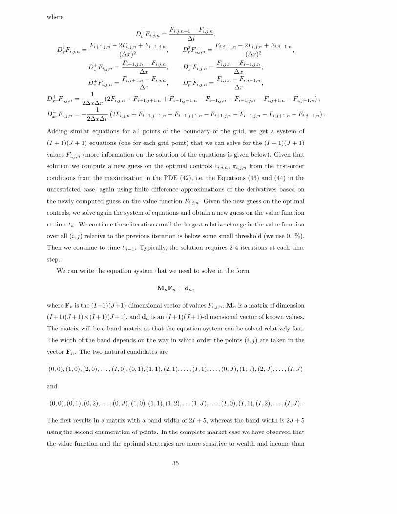
where
D+t Fi,j,n =
Fi,j,n+1 − Fi,j,n
∆t,
D2xFi,j,n =
Fi+1,j,n − 2Fi,j,n + Fi−1,j,n
(∆x)2, D2
rFi,j,n =Fi,j+1,n − 2Fi,j,n + Fi,j−1,n
(∆r)2,
D+x Fi,j,n =
Fi+1,j,n − Fi,j,n
∆x, D−
x Fi,j,n =Fi,j,n − Fi−1,j,n
∆x,
D+r Fi,j,n =
Fi,j+1,n − Fi,j,n
∆r, D−
r Fi,j,n =Fi,j,n − Fi,j−1,n
∆r,
D+xrFi,j,n =
1
2∆x∆r(2Fi,j,n + Fi+1,j+1,n + Fi−1,j−1,n − Fi+1,j,n − Fi−1,j,n − Fi,j+1,n − Fi,j−1,n) ,
D−xrFi,j,n = − 1
2∆x∆r(2Fi,j,n + Fi+1,j−1,n + Fi−1,j+1,n − Fi+1,j,n − Fi−1,j,n − Fi,j+1,n − Fi,j−1,n) .
Adding similar equations for all points of the boundary of the grid, we get a system of
(I + 1)(J + 1) equations (one for each grid point) that we can solve for the (I + 1)(J + 1)
values Fi,j,n (more information on the solution of the equations is given below). Given that
solution we compute a new guess on the optimal controls ci,j,n, πi,j,n from the first-order
conditions from the maximization in the PDE (42), i.e. the Equations (43) and (44) in the
unrestricted case, again using finite difference approximations of the derivatives based on
the newly computed guess on the value function Fi,j,n. Given the new guess on the optimal
controls, we solve again the system of equations and obtain a new guess on the value function
at time tn. We continue these iterations until the largest relative change in the value function
over all (i, j) relative to the previous iteration is below some small threshold (we use 0.1%).
Then we continue to time tn−1. Typically, the solution requires 2-4 iterations at each time
step.
We can write the equation system that we need to solve in the form
MnFn = dn,
where Fn is the (I+1)(J+1)-dimensional vector of values Fi,j,n, Mn is a matrix of dimension
(I+1)(J+1)×(I+1)(J+1), and dn is an (I+1)(J+1)-dimensional vector of known values.
The matrix will be a band matrix so that the equation system can be solved relatively fast.
The width of the band depends on the way in which order the points (i, j) are taken in the
vector Fn. The two natural candidates are
(0, 0), (1, 0), (2, 0), . . . , (I, 0), (0, 1), (1, 1), (2, 1), . . . , (I, 1), . . . , (0, J), (1, J), (2, J), . . . , (I, J)
and
(0, 0), (0, 1), (0, 2), . . . , (0, J), (1, 0), (1, 1), (1, 2), . . . (1, J), . . . , (I, 0), (I, 1), (I, 2), . . . , (I, J).
The first results in a matrix with a band width of 2I + 5, whereas the band width is 2J + 5
using the second enumeration of points. In the complete market case we have observed that
the value function and the optimal strategies are more sensitive to wealth and income than
35

to the interest rate, and since we expect the same in the incomplete market case, we will use
I > J . Therefore the second enumeration is more efficient, both in relation to the number
of non-zero values to store in the computer and in relation to the speed with which the
equation system can be solved.
The numerical results stated in Section 5 are based on an implementation of the above
procedure with I = 500, J = 40, and four time steps per year. The imposed bounds are
xI = 10, r0 = −0.03, and rJ = 0.07.
36
References
Bodie, Z., R. C. Merton, and W. F. Samuelson (1992). Labor Supply Flexibility and
Portfolio Choice in a Life Cycle Model. Journal of Economic Dynamics and Control 16,
427–449.
Brennan, M. J., E. S. Schwartz, and R. Lagnado (1997). Strategic Asset Allocation.
Journal of Economic Dynamics and Control 21 (8–9), 1377–1403.
Brennan, M. J. and Y. Xia (2000). Stochastic Interest Rates and the Bond-Stock Mix.
European Finance Review 4 (2), 197–210.
Brennan, M. J. and Y. Xia (2002). Dynamic Asset Allocation under Inflation. The Journal
of Finance 57 (3), 1201–1238.
Campbell, J. Y. and L. M. Viceira (2001). Who Should Buy Long-Term Bonds? American
Economic Review 91 (1), 99–127.
Campbell, J. Y. and L. M. Viceira (2002). Strategic Asset Allocation. Oxford University
Press.
Chan, Y. L. and L. M. Viceira (2000, December). Asset Allocation with Endogenous
Labor Income: The Case of Incomplete Markets. Working paper.
Cocco, J. F., F. J. Gomes, and P. J. Maenhout (2005). Consumption and Portfolio Choice
over the Life-Cycle. Forthcoming in the Review of Financial Studies.
Constantinides, G. M., J. B. Donaldson, and R. Mehra (2002). Junior Can’t Borrow: A
New Perspective on the Equity Premium Puzzle. Quarterly Journal of Economics 117,
269–296.
Davis, S. J., F. Kubler, and P. Willen (2003, October). Borrowing Costs and the Demand
for Equity over the Life Cycle. Working paper, University of Chicago and Stanford
University.
Davis, S. J. and P. Willen (2000, March). Using Financial Assets to Hedge Labor Income
Risks: Estimating the Benefits. Working paper, University of Chicago and Princeton
University.
Detemple, J., R. Garcia, and M. Rindisbacher (2003). A Monte-Carlo Method for Optimal
Portfolios. The Journal of Finance 58 (1), 401–446.
Dimson, E., P. Marsh, and M. Staunton (2002). Triumph of the Optimists: 101 Years of
Global Investment Returns. Princeton University Press.
Duffie, D., W. Fleming, H. M. Soner, and T. Zariphopoulou (1997). Hedging in Incomplete
Markets with HARA Utility. Journal of Economic Dynamics and Control 21 (4–5),
753–782.
37
Duffie, D., J. Pan, and K. Singleton (2000). Transform Analysis and Asset Pricing for
Affine Jump-Diffusions. Econometrica 68 (6), 1343–1376.
El Karoui, N. and M. Jeanblanc-Picque (1998). Optimization of Consumption with Labor
Income. Finance and Stochastics 2 (4), 409–440.
Fitzpatrick, B. G. and W. H. Fleming (1991). Numerical Methods for an Optimal
Investment-Consumption Model. Mathematics of Operations Research 16 (4), 823–841.
Hakansson, N. H. (1970). Optimal Investment and Consumption Strategies Under Risk
for a Class of Utility Functions. Econometrica 38 (5), 587–607.
He, H. and H. F. Pages (1993). Labor Income, Borrowing Constraints, and Equilibrium
Asset Prices. Economic Theory 3, 663–696.
Heaton, J. and D. Lucas (1997). Market Frictions, Savings Behavior, and Portfolio Choice.
Macroeconomic Dynamics 1, 76–101.
Heaton, J. and D. Lucas (2000). Portfolio Choice and Asset Prices: The Importance of
Entrepreneurial Risk. The Journal of Finance 55 (3), 1163–1198.
Hindy, A., C.-f. Huang, and H. Zhu (1997). Numerical Analysis of a Free-Boundary Sin-
gular Control Problem in Financial Economics. Journal of Economic Dynamics and
Control 21 (2–3), 297–327.
Hubbard, R. G., J. Skinner, and S. P. Zeldes (1995). Precautionary Saving and Social
Insurance. Journal of Political Economy 103 (2), 360–399.
Ingersoll, Jr., J. E. (1987). Theory of Financial Decision Making. Rowman & Littlefield.
Jagannathan, R. and Z. Wang (1996). The Conditional CAPM and the Cross-Section of
Expected Returns. The Journal of Finance 51 (1), 3–53.
Julliard, C. (2004, October). Labor Income Risk and Asset Returns. Working paper,
Princeton University.
Karatzas, I. and S. E. Shreve (1988). Brownian Motion and Stochastic Calculus, Volume
113 of Graduate Texts in Mathematics. New York, New York, USA: Springer-Verlag.
Koo, H. K. (1998). Consumption and Portfolio Selection with Labor Income: A Contin-
uous Time Approach. Mathematical Finance 8 (1), 49–65.
Liu, J. (1999, August). Portfolio Selection in Stochastic Environments. Working paper,
Stanford University.
Merton, R. C. (1971). Optimum Consumption and Portfolio Rules in a Continuous-Time
Model. Journal of Economic Theory 3, 373–413. Erratum: Merton (1973). Reprinted
as Chapter 5 in Merton (1992).
Merton, R. C. (1973). Erratum. Journal of Economic Theory 6, 213–214.
38

Merton, R. C. (1992). Continuous-Time Finance. Padstow, UK: Basil Blackwell Inc.
Munk, C. (1999). The Valuation of Contingent Claims under Portfolio Constraints: Reser-
vation Buying and Selling Prices. European Finance Review 3 (3), 347–388.
Munk, C. (2000). Optimal Consumption-Investment Policies with Undiversifiable Income
Risk and Liquidity Constraints. Journal of Economic Dynamics and Control 24 (9),
1315–1343.
Munk, C. and C. Sørensen (2004). Optimal Consumption and Investment Strategies with
Stochastic Interest Rates. Journal of Banking and Finance 28 (8), 1987–2013.
Munk, C., C. Sørensen, and T. N. Vinther (2004). Dynamic Asset Allocation Under Mean-
Reverting Returns, Stochastic Interest Rates and Inflation Uncertainty. International
Review of Economics and Finance 13 (2), 141–166.
Shiller, R. J. (2000). Irrational Exuberance. Princeton, New Jersey: Princeton University
Press.
Sørensen, C. (1999). Dynamic Asset Allocation and Fixed Income Management. Journal
of Financial and Quantitative Analysis 34, 513–531.
Storesletten, K., C. I. Telmer, and A. Yaron (2004). Cyclical Dynamics in Idiosyncratic
Labor Market Risk. Journal of Political Economy 112 (3), 695–717.
Vasicek, O. (1977). An Equilibrium Characterization of the Term Structure. Journal of
Financial Economics 5, 177–188.
Viceira, L. M. (2001). Optimal Portfolio Choice for Long-Horizon Investors with Nontrad-
able Labor Income. The Journal of Finance 56 (2), 433–470.
39
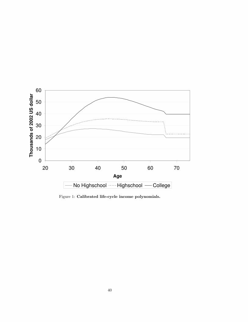
0
10
20
30
40
50
60
20 30 40 50 60 70
Age
Th
ou
sa
nd
s o
f 2
00
2 U
S d
oll
ar
No Highschool Highschool College
Figure 1: Calibrated life-cycle income polynomials.
40
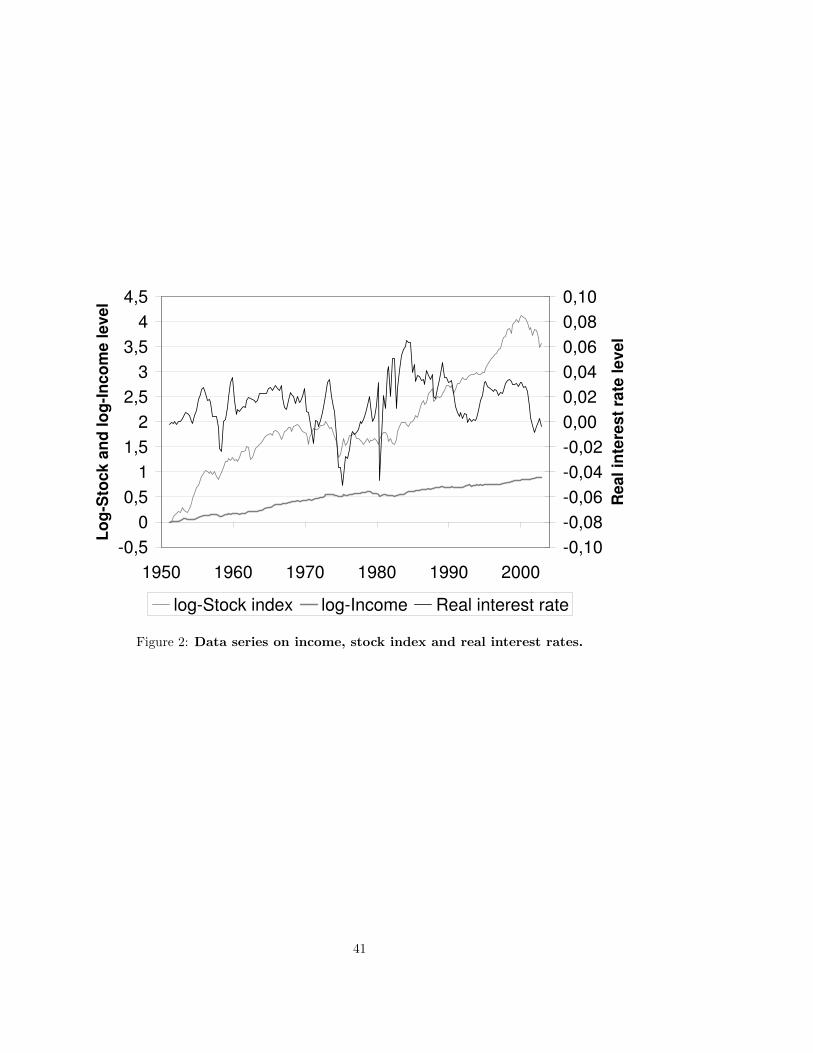
-0,5
0
0,5
1
1,5
2
2,5
3
3,5
4
4,5
1950 1960 1970 1980 1990 2000
Lo
g-S
tock a
nd
lo
g-I
nco
me level
-0,10
-0,08
-0,06
-0,04
-0,02
0,00
0,02
0,04
0,06
0,08
0,10
Real in
tere
st
rate
level
log-Stock index log-Income Real interest rate
Figure 2: Data series on income, stock index and real interest rates.
41
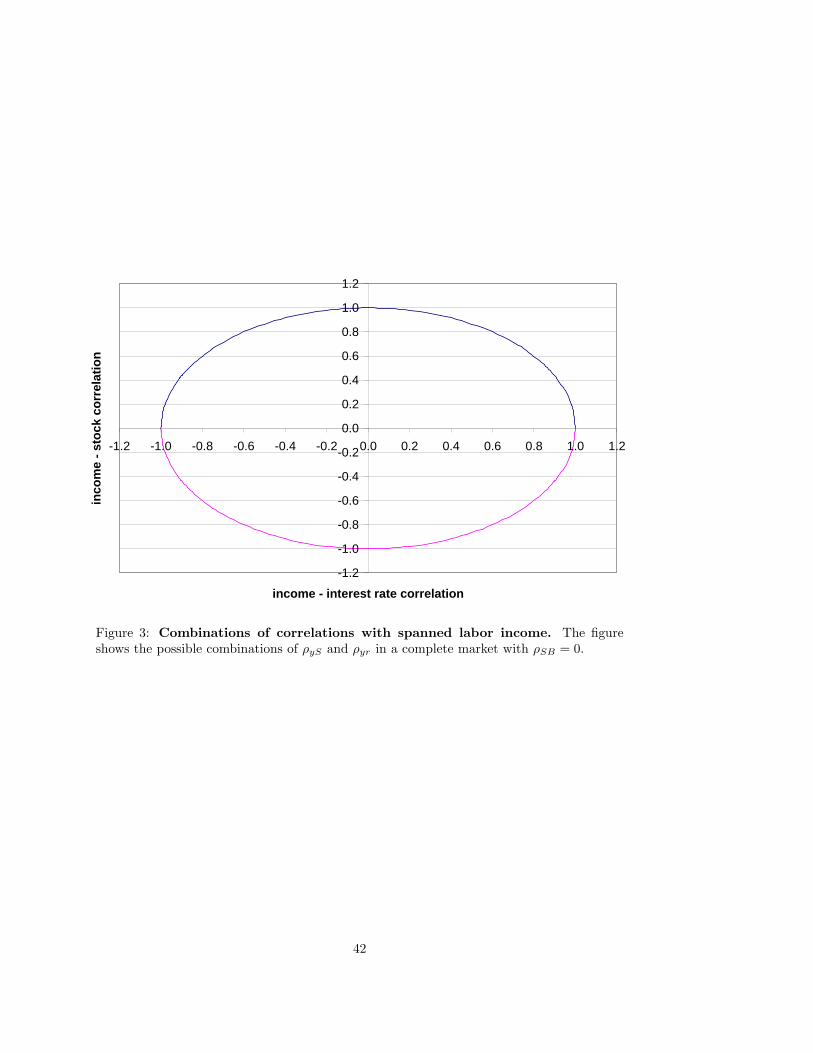
-1.2
-1.0
-0.8
-0.6
-0.4
-0.2
0.0
0.2
0.4
0.6
0.8
1.0
1.2
-1.2 -1.0 -0.8 -0.6 -0.4 -0.2 0.0 0.2 0.4 0.6 0.8 1.0 1.2
income - interest rate correlation
inco
me
- st
ock
co
rrel
atio
n
Figure 3: Combinations of correlations with spanned labor income. The figureshows the possible combinations of ρyS and ρyr in a complete market with ρSB = 0.
42
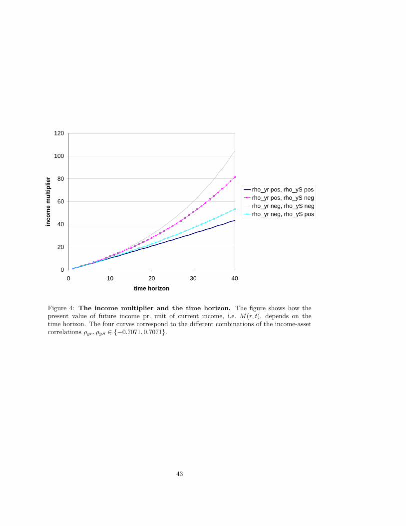
0
20
40
60
80
100
120
0 10 20 30 40
time horizon
inco
me
mu
ltip
lier
rho_yr pos, rho_yS posrho_yr pos, rho_yS negrho_yr neg, rho_yS negrho_yr neg, rho_yS pos
Figure 4: The income multiplier and the time horizon. The figure shows how thepresent value of future income pr. unit of current income, i.e. M(r, t), depends on thetime horizon. The four curves correspond to the different combinations of the income-assetcorrelations ρyr, ρyS ∈ −0.7071, 0.7071.
43
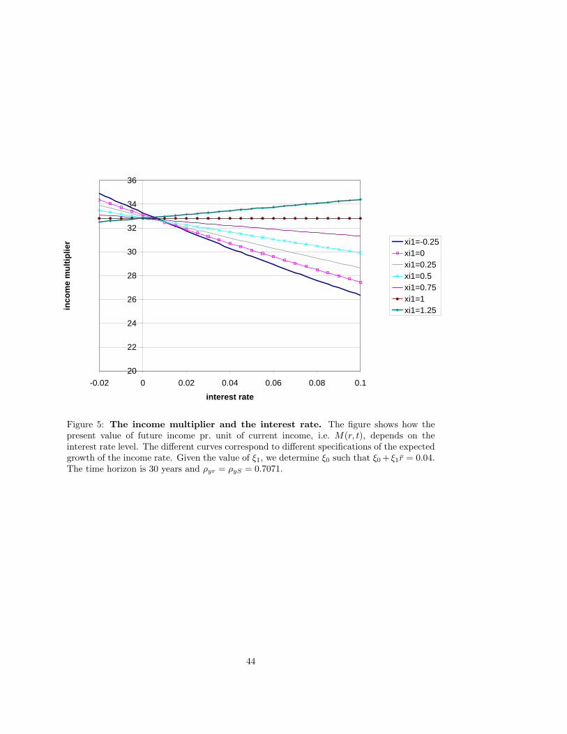
20
22
24
26
28
30
32
34
36
-0.02 0 0.02 0.04 0.06 0.08 0.1
interest rate
inco
me
mu
ltip
lier xi1=-0.25
xi1=0xi1=0.25xi1=0.5xi1=0.75xi1=1xi1=1.25
Figure 5: The income multiplier and the interest rate. The figure shows how thepresent value of future income pr. unit of current income, i.e. M(r, t), depends on theinterest rate level. The different curves correspond to different specifications of the expectedgrowth of the income rate. Given the value of ξ1, we determine ξ0 such that ξ0 + ξ1r = 0.04.The time horizon is 30 years and ρyr = ρyS = 0.7071.
44
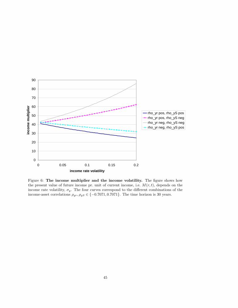
0
10
20
30
40
50
60
70
80
90
0 0.05 0.1 0.15 0.2
income rate volatility
inco
me
mu
ltip
lier
rho_yr pos, rho_yS posrho_yr pos, rho_yS negrho_yr neg, rho_yS negrho_yr neg, rho_yS pos
Figure 6: The income multiplier and the income volatility. The figure shows howthe present value of future income pr. unit of current income, i.e. M(r, t), depends on theincome rate volatility, σy. The four curves correspond to the different combinations of theincome-asset correlations ρyr, ρyS ∈ −0.7071, 0.7071. The time horizon is 30 years.
45
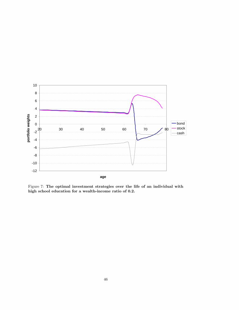
-12
-10
-8
-6
-4
-2
0
2
4
6
8
10
20 30 40 50 60 70 80
age
po
rtfo
lio w
eig
hts
bondstockcash
Figure 7: The optimal investment strategies over the life of an individual with
high school education for a wealth-income ratio of 0.2.
46
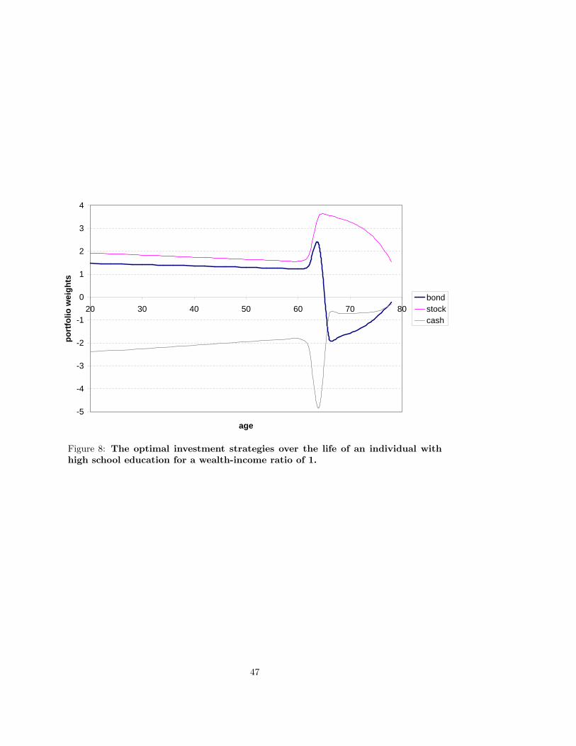
-5
-4
-3
-2
-1
0
1
2
3
4
20 30 40 50 60 70 80
age
po
rtfo
lio w
eig
hts
bondstockcash
Figure 8: The optimal investment strategies over the life of an individual with
high school education for a wealth-income ratio of 1.
47
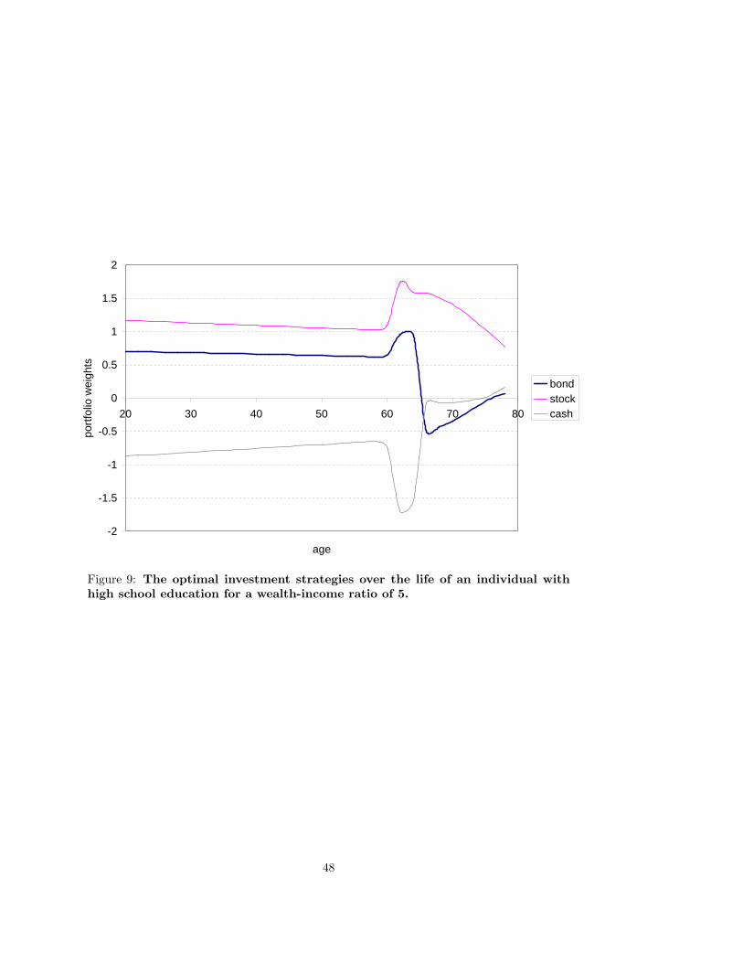
-2
-1.5
-1
-0.5
0
0.5
1
1.5
2
20 30 40 50 60 70 80
age
port
folio
wei
ghts
bondstockcash
Figure 9: The optimal investment strategies over the life of an individual with
high school education for a wealth-income ratio of 5.
48
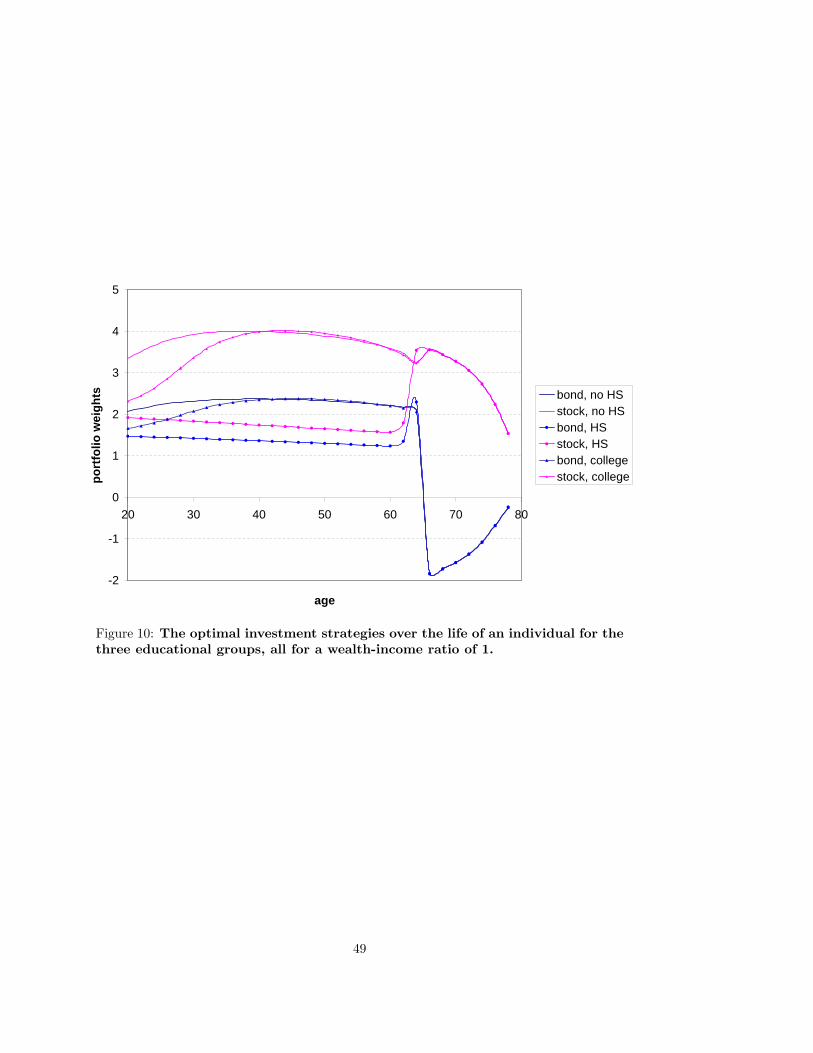
-2
-1
0
1
2
3
4
5
20 30 40 50 60 70 80
age
po
rtfo
lio w
eig
hts bond, no HS
stock, no HSbond, HSstock, HSbond, collegestock, college
Figure 10: The optimal investment strategies over the life of an individual for the
three educational groups, all for a wealth-income ratio of 1.
49

No High school High school College
ai -2.1361 -2.1700 -4.3148
bi 0.1684 0.1682 0.3194
ci -0.00353 -0.00323 -0.00577
di 0.000023 0.000020 0.000033
P i 0.88983 0.68212 0.93887
Initial age 20 level 17,763 19,107 13,912(in 2002 US dollar)
Table 1: Coefficients in the life-cycle income polynomials.
50
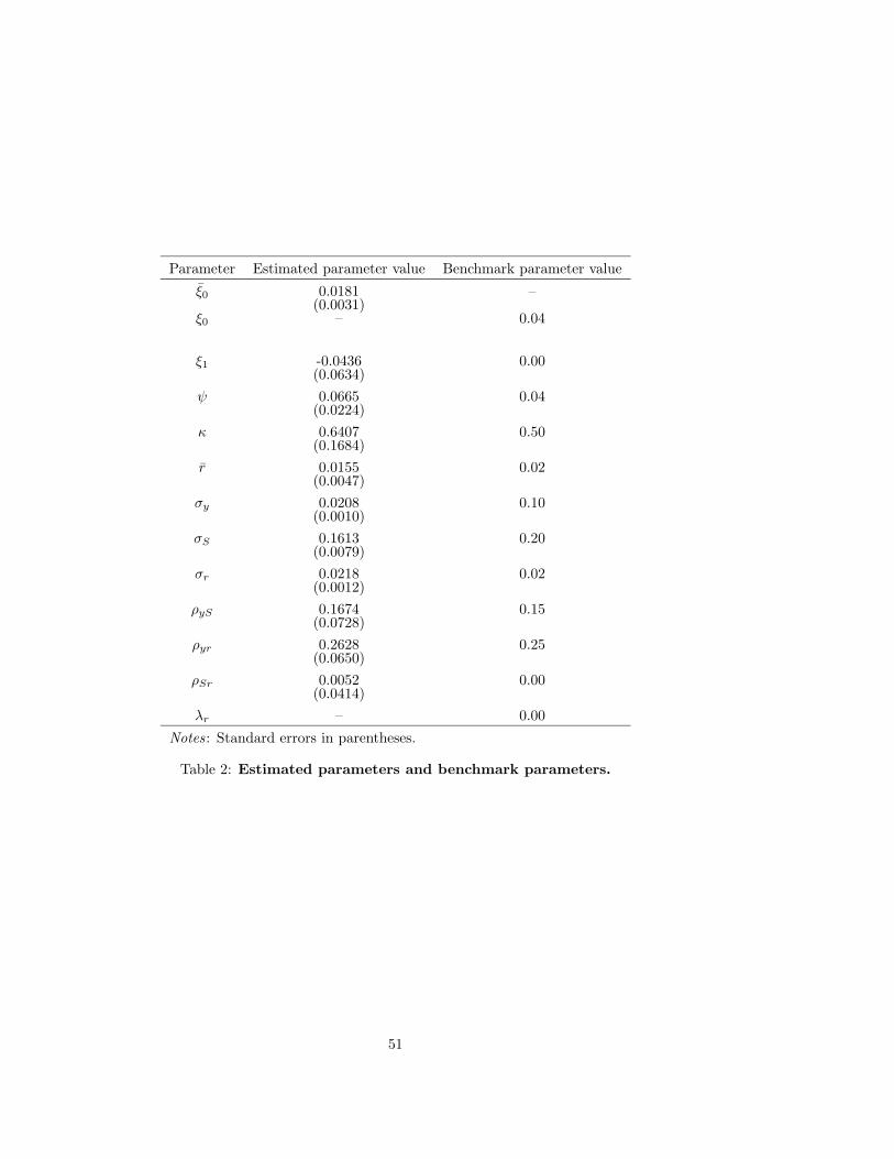
Parameter Estimated parameter value Benchmark parameter value
ξ0 0.0181 –(0.0031)
ξ0 – 0.04
ξ1 -0.0436 0.00(0.0634)
ψ 0.0665 0.04(0.0224)
κ 0.6407 0.50(0.1684)
r 0.0155 0.02(0.0047)
σy 0.0208 0.10(0.0010)
σS 0.1613 0.20(0.0079)
σr 0.0218 0.02(0.0012)
ρyS 0.1674 0.15(0.0728)
ρyr 0.2628 0.25(0.0650)
ρSr 0.0052 0.00(0.0414)
λr – 0.00
Notes: Standard errors in parentheses.
Table 2: Estimated parameters and benchmark parameters.
51
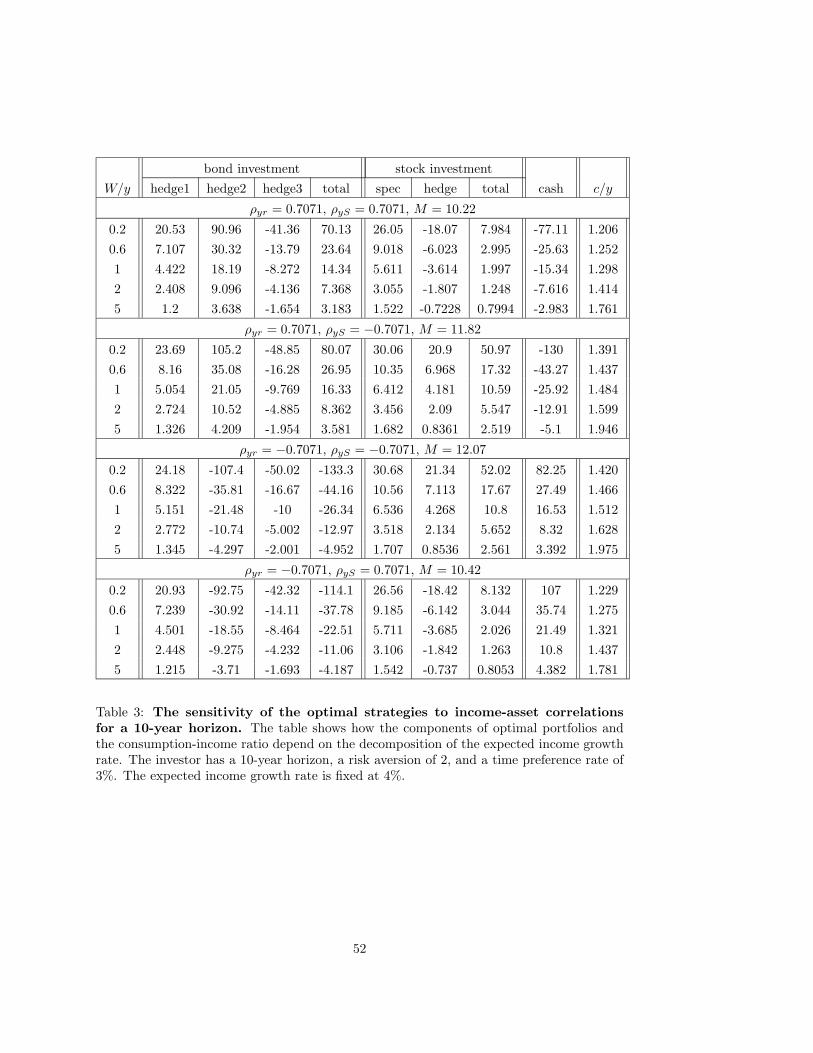
bond investment stock investment
W/y hedge1 hedge2 hedge3 total spec hedge total cash c/y
ρyr = 0.7071, ρyS = 0.7071, M = 10.22
0.2 20.53 90.96 -41.36 70.13 26.05 -18.07 7.984 -77.11 1.206
0.6 7.107 30.32 -13.79 23.64 9.018 -6.023 2.995 -25.63 1.252
1 4.422 18.19 -8.272 14.34 5.611 -3.614 1.997 -15.34 1.298
2 2.408 9.096 -4.136 7.368 3.055 -1.807 1.248 -7.616 1.414
5 1.2 3.638 -1.654 3.183 1.522 -0.7228 0.7994 -2.983 1.761
ρyr = 0.7071, ρyS = −0.7071, M = 11.82
0.2 23.69 105.2 -48.85 80.07 30.06 20.9 50.97 -130 1.391
0.6 8.16 35.08 -16.28 26.95 10.35 6.968 17.32 -43.27 1.437
1 5.054 21.05 -9.769 16.33 6.412 4.181 10.59 -25.92 1.484
2 2.724 10.52 -4.885 8.362 3.456 2.09 5.547 -12.91 1.599
5 1.326 4.209 -1.954 3.581 1.682 0.8361 2.519 -5.1 1.946
ρyr = −0.7071, ρyS = −0.7071, M = 12.07
0.2 24.18 -107.4 -50.02 -133.3 30.68 21.34 52.02 82.25 1.420
0.6 8.322 -35.81 -16.67 -44.16 10.56 7.113 17.67 27.49 1.466
1 5.151 -21.48 -10 -26.34 6.536 4.268 10.8 16.53 1.512
2 2.772 -10.74 -5.002 -12.97 3.518 2.134 5.652 8.32 1.628
5 1.345 -4.297 -2.001 -4.952 1.707 0.8536 2.561 3.392 1.975
ρyr = −0.7071, ρyS = 0.7071, M = 10.42
0.2 20.93 -92.75 -42.32 -114.1 26.56 -18.42 8.132 107 1.229
0.6 7.239 -30.92 -14.11 -37.78 9.185 -6.142 3.044 35.74 1.275
1 4.501 -18.55 -8.464 -22.51 5.711 -3.685 2.026 21.49 1.321
2 2.448 -9.275 -4.232 -11.06 3.106 -1.842 1.263 10.8 1.437
5 1.215 -3.71 -1.693 -4.187 1.542 -0.737 0.8053 4.382 1.781
Table 3: The sensitivity of the optimal strategies to income-asset correlations
for a 10-year horizon. The table shows how the components of optimal portfolios andthe consumption-income ratio depend on the decomposition of the expected income growthrate. The investor has a 10-year horizon, a risk aversion of 2, and a time preference rate of3%. The expected income growth rate is fixed at 4%.
52
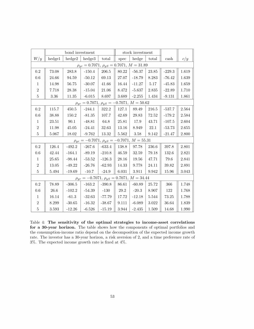
bond investment stock investment
W/y hedge1 hedge2 hedge3 total spec hedge total cash c/y
ρyr = 0.7071, ρyS = 0.7071, M = 31.89
0.2 73.08 283.8 -150.4 206.5 80.22 -56.37 23.85 -229.3 1.619
0.6 24.66 94.59 -50.12 69.13 27.07 -18.79 8.283 -76.42 1.639
1 14.98 56.75 -30.07 41.66 16.44 -11.27 5.17 -45.83 1.659
2 7.718 28.38 -15.04 21.06 8.472 -5.637 2.835 -22.89 1.710
5 3.36 11.35 -6.015 8.697 3.689 -2.255 1.434 -9.131 1.861
ρyr = 0.7071, ρyS = −0.7071, M = 50.62
0.2 115.7 450.5 -244.1 322.2 127.1 89.49 216.5 -537.7 2.564
0.6 38.88 150.2 -81.35 107.7 42.69 29.83 72.52 -179.2 2.584
1 23.51 90.1 -48.81 64.8 25.81 17.9 43.71 -107.5 2.604
2 11.98 45.05 -24.41 32.63 13.16 8.949 22.1 -53.73 2.655
5 5.067 18.02 -9.762 13.32 5.562 3.58 9.142 -21.47 2.800
ρyr = −0.7071, ρyS = −0.7071, M = 55.31
0.2 126.4 -492.2 -267.6 -633.4 138.8 97.78 236.6 397.8 2.801
0.6 42.44 -164.1 -89.19 -210.8 46.59 32.59 79.18 132.6 2.821
1 25.65 -98.44 -53.52 -126.3 28.16 19.56 47.71 79.6 2.841
2 13.05 -49.22 -26.76 -62.93 14.33 9.778 24.11 39.82 2.891
5 5.494 -19.69 -10.7 -24.9 6.031 3.911 9.942 15.96 3.043
ρyr = −0.7071, ρyS = 0.7071, M = 34.44
0.2 78.89 -306.5 -163.2 -390.8 86.61 -60.89 25.72 366 1.748
0.6 26.6 -102.2 -54.39 -130 29.2 -20.3 8.907 122 1.768
1 16.14 -61.3 -32.63 -77.79 17.72 -12.18 5.544 73.25 1.788
2 8.299 -30.65 -16.32 -38.67 9.111 -6.089 3.022 36.64 1.839
5 3.593 -12.26 -6.526 -15.19 3.944 -2.435 1.509 14.68 1.990
Table 4: The sensitivity of the optimal strategies to income-asset correlations
for a 30-year horizon. The table shows how the components of optimal portfolios andthe consumption-income ratio depend on the decomposition of the expected income growthrate. The investor has a 30-year horizon, a risk aversion of 2, and a time preference rate of3%. The expected income growth rate is fixed at 4%.
53

bond investment stock investment
W/y hedge1 hedge2 hedge3 total spec hedge total cash c/y
ξ0 = 0.045, ξ1 = −0.25, M = 10.21
0.2 20.51 90.85 -51.63 59.73 26.02 -18.05 7.976 -66.7 1.204
0.6 7.099 30.28 -17.21 20.17 9.008 -6.016 2.992 -22.16 1.251
1 4.417 18.17 -10.33 12.26 5.605 -3.61 1.995 -13.26 1.297
2 2.405 9.085 -5.163 6.327 3.052 -1.805 1.248 -6.575 1.412
5 1.199 3.634 -2.065 2.767 1.521 -0.7219 0.799 -2.566 1.760
ξ0 = 0.035, ξ1 = 0.25, M = 10.24
0.2 20.56 91.09 -31.07 80.58 26.09 -18.1 7.996 -87.58 1.207
0.6 7.117 30.36 -10.36 27.12 9.03 -6.032 2.999 -29.12 1.254
1 4.428 18.22 -6.215 16.43 5.618 -3.619 1.999 -17.43 1.300
2 2.411 9.109 -3.107 8.413 3.059 -1.81 1.25 -8.662 1.416
5 1.201 3.644 -1.243 3.601 1.524 -0.7238 0.7998 -3.401 1.763
ξ0 = 0.025, ξ1 = 0.75, M = 10.28
0.2 20.64 91.44 -10.4 101.7 26.19 -18.16 8.024 -108.7 1.212
0.6 7.142 30.48 -3.468 34.15 9.063 -6.055 3.008 -36.16 1.258
1 4.443 18.29 -2.081 20.65 5.638 -3.633 2.005 -21.65 1.304
2 2.418 9.144 -1.04 10.52 3.069 -1.816 1.252 -10.77 1.420
5 1.204 3.657 -0.4162 4.445 1.528 -0.7266 0.801 -4.246 1.767
ξ0 = 0.015, ξ1 = 1.25, M = 10.33
0.2 20.74 91.88 10.46 123.1 26.31 -18.25 8.06 -130.1 1.218
0.6 7.175 30.63 3.488 41.29 9.104 -6.084 3.02 -43.31 1.264
1 4.463 18.38 2.093 24.93 5.663 -3.651 2.012 -25.94 1.310
2 2.428 9.188 1.046 12.66 3.081 -1.825 1.256 -12.92 1.426
5 1.208 3.675 0.4185 5.302 1.533 -0.7301 0.8024 -5.104 1.773
Table 5: The sensitivity of the optimal strategies to the decomposition of the
expected income growth rate. The table shows how the components of optimal portfoliosand the consumption-income ratio depend on the decomposition of the expected incomegrowth rate. The investor has a 10-year horizon, a risk aversion of 2, and a time preferencerate of 3%. The income-asset correlations are ρyr = ρyS =
√2/2.
54
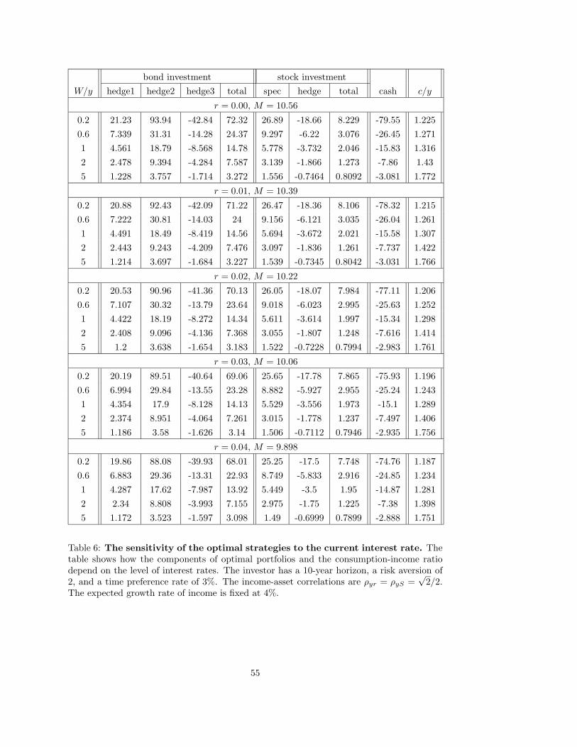
bond investment stock investment
W/y hedge1 hedge2 hedge3 total spec hedge total cash c/y
r = 0.00, M = 10.56
0.2 21.23 93.94 -42.84 72.32 26.89 -18.66 8.229 -79.55 1.225
0.6 7.339 31.31 -14.28 24.37 9.297 -6.22 3.076 -26.45 1.271
1 4.561 18.79 -8.568 14.78 5.778 -3.732 2.046 -15.83 1.316
2 2.478 9.394 -4.284 7.587 3.139 -1.866 1.273 -7.86 1.43
5 1.228 3.757 -1.714 3.272 1.556 -0.7464 0.8092 -3.081 1.772
r = 0.01, M = 10.39
0.2 20.88 92.43 -42.09 71.22 26.47 -18.36 8.106 -78.32 1.215
0.6 7.222 30.81 -14.03 24 9.156 -6.121 3.035 -26.04 1.261
1 4.491 18.49 -8.419 14.56 5.694 -3.672 2.021 -15.58 1.307
2 2.443 9.243 -4.209 7.476 3.097 -1.836 1.261 -7.737 1.422
5 1.214 3.697 -1.684 3.227 1.539 -0.7345 0.8042 -3.031 1.766
r = 0.02, M = 10.22
0.2 20.53 90.96 -41.36 70.13 26.05 -18.07 7.984 -77.11 1.206
0.6 7.107 30.32 -13.79 23.64 9.018 -6.023 2.995 -25.63 1.252
1 4.422 18.19 -8.272 14.34 5.611 -3.614 1.997 -15.34 1.298
2 2.408 9.096 -4.136 7.368 3.055 -1.807 1.248 -7.616 1.414
5 1.2 3.638 -1.654 3.183 1.522 -0.7228 0.7994 -2.983 1.761
r = 0.03, M = 10.06
0.2 20.19 89.51 -40.64 69.06 25.65 -17.78 7.865 -75.93 1.196
0.6 6.994 29.84 -13.55 23.28 8.882 -5.927 2.955 -25.24 1.243
1 4.354 17.9 -8.128 14.13 5.529 -3.556 1.973 -15.1 1.289
2 2.374 8.951 -4.064 7.261 3.015 -1.778 1.237 -7.497 1.406
5 1.186 3.58 -1.626 3.14 1.506 -0.7112 0.7946 -2.935 1.756
r = 0.04, M = 9.898
0.2 19.86 88.08 -39.93 68.01 25.25 -17.5 7.748 -74.76 1.187
0.6 6.883 29.36 -13.31 22.93 8.749 -5.833 2.916 -24.85 1.234
1 4.287 17.62 -7.987 13.92 5.449 -3.5 1.95 -14.87 1.281
2 2.34 8.808 -3.993 7.155 2.975 -1.75 1.225 -7.38 1.398
5 1.172 3.523 -1.597 3.098 1.49 -0.6999 0.7899 -2.888 1.751
Table 6: The sensitivity of the optimal strategies to the current interest rate. Thetable shows how the components of optimal portfolios and the consumption-income ratiodepend on the level of interest rates. The investor has a 10-year horizon, a risk aversion of2, and a time preference rate of 3%. The income-asset correlations are ρyr = ρyS =
√2/2.
The expected growth rate of income is fixed at 4%.
55
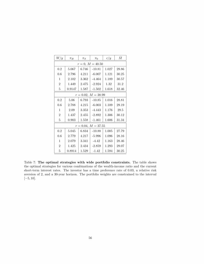
W/y πB πS π0 c/y M
r = 0, M = 40.50
0.2 5.067 6.746 -10.81 1.027 29.86
0.6 2.796 4.211 -6.007 1.121 30.25
1 2.102 3.362 -4.464 1.189 30.57
2 1.449 2.475 -2.924 1.32 31.2
5 0.9147 1.587 -1.502 1.618 32.46
r = 0.02, M = 38.99
0.2 5.06 6.793 -10.85 1.016 28.81
0.6 2.788 4.215 -6.003 1.109 29.19
1 2.09 3.353 -4.443 1.176 29.5
2 1.437 2.455 -2.892 1.306 30.12
5 0.903 1.558 -1.461 1.606 31.34
r = 0.04, M = 37.55
0.2 5.045 6.834 -10.88 1.005 27.79
0.6 2.779 4.217 -5.996 1.096 28.16
1 2.079 3.341 -4.42 1.163 28.46
2 1.425 2.434 -2.859 1.293 29.07
5 0.8914 1.529 -1.42 1.594 30.25
Table 7: The optimal strategies with wide portfolio constraints. The table showsthe optimal strategies for various combinations of the wealth-income ratio and the currentshort-term interest rates. The investor has a time preference rate of 0.03, a relative riskaversion of 2, and a 30-year horizon. The portfolio weights are constrained to the interval[−5, 10].
56
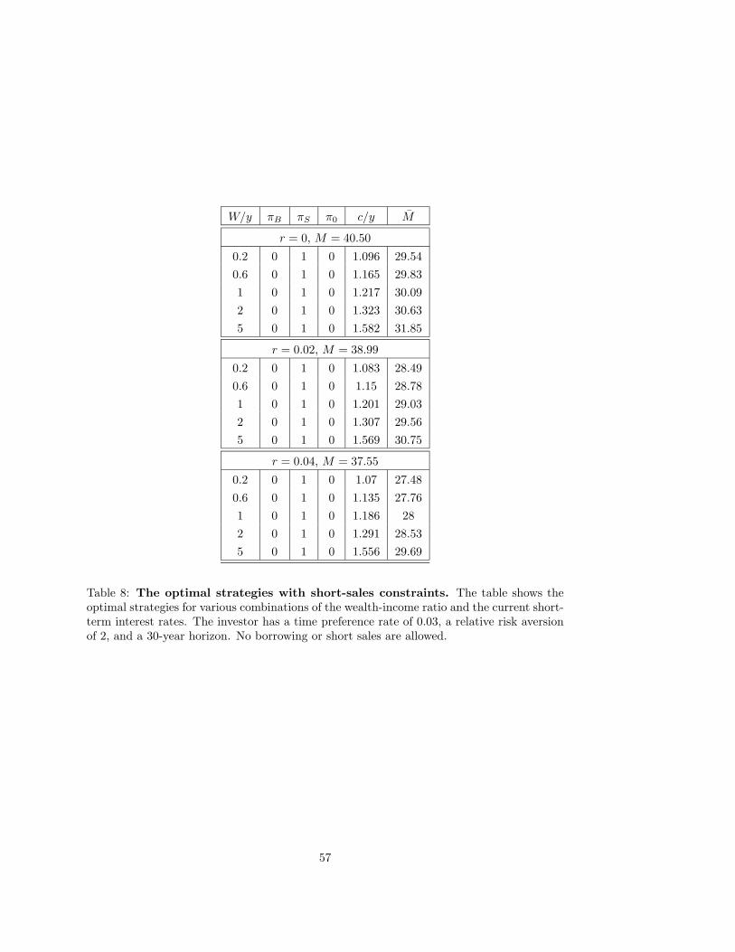
W/y πB πS π0 c/y M
r = 0, M = 40.50
0.2 0 1 0 1.096 29.54
0.6 0 1 0 1.165 29.83
1 0 1 0 1.217 30.09
2 0 1 0 1.323 30.63
5 0 1 0 1.582 31.85
r = 0.02, M = 38.99
0.2 0 1 0 1.083 28.49
0.6 0 1 0 1.15 28.78
1 0 1 0 1.201 29.03
2 0 1 0 1.307 29.56
5 0 1 0 1.569 30.75
r = 0.04, M = 37.55
0.2 0 1 0 1.07 27.48
0.6 0 1 0 1.135 27.76
1 0 1 0 1.186 28
2 0 1 0 1.291 28.53
5 0 1 0 1.556 29.69
Table 8: The optimal strategies with short-sales constraints. The table shows theoptimal strategies for various combinations of the wealth-income ratio and the current short-term interest rates. The investor has a time preference rate of 0.03, a relative risk aversionof 2, and a 30-year horizon. No borrowing or short sales are allowed.
57
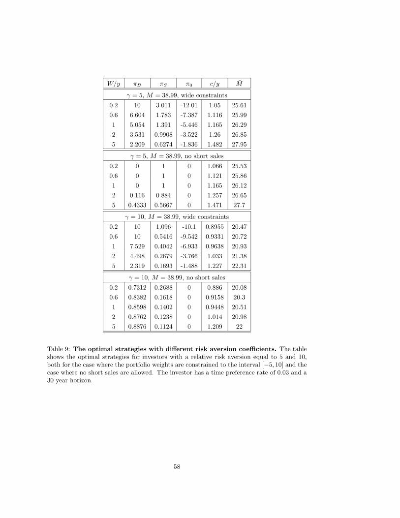
W/y πB πS π0 c/y M
γ = 5, M = 38.99, wide constraints
0.2 10 3.011 -12.01 1.05 25.61
0.6 6.604 1.783 -7.387 1.116 25.99
1 5.054 1.391 -5.446 1.165 26.29
2 3.531 0.9908 -3.522 1.26 26.85
5 2.209 0.6274 -1.836 1.482 27.95
γ = 5, M = 38.99, no short sales
0.2 0 1 0 1.066 25.53
0.6 0 1 0 1.121 25.86
1 0 1 0 1.165 26.12
2 0.116 0.884 0 1.257 26.65
5 0.4333 0.5667 0 1.471 27.7
γ = 10, M = 38.99, wide constraints
0.2 10 1.096 -10.1 0.8955 20.47
0.6 10 0.5416 -9.542 0.9331 20.72
1 7.529 0.4042 -6.933 0.9638 20.93
2 4.498 0.2679 -3.766 1.033 21.38
5 2.319 0.1693 -1.488 1.227 22.31
γ = 10, M = 38.99, no short sales
0.2 0.7312 0.2688 0 0.886 20.08
0.6 0.8382 0.1618 0 0.9158 20.3
1 0.8598 0.1402 0 0.9448 20.51
2 0.8762 0.1238 0 1.014 20.98
5 0.8876 0.1124 0 1.209 22
Table 9: The optimal strategies with different risk aversion coefficients. The tableshows the optimal strategies for investors with a relative risk aversion equal to 5 and 10,both for the case where the portfolio weights are constrained to the interval [−5, 10] and thecase where no short sales are allowed. The investor has a time preference rate of 0.03 and a30-year horizon.
58
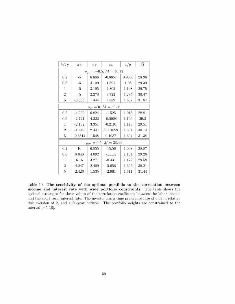
W/y πB πS π0 c/y M
ρyr = −0.5, M = 40.72
0.2 -5 6.886 -0.8857 0.9886 28.96
0.6 -5 4.109 1.891 1.08 29.39
1 -5 3.195 2.805 1.148 29.75
2 -5 2.278 3.722 1.285 30.47
5 -3.333 1.444 2.889 1.607 31.87
ρyr = 0, M = 39.56
0.2 -4.299 6.824 -1.525 1.013 28.81
0.6 -2.721 4.222 -0.5008 1.106 29.2
1 -2.132 3.351 -0.2191 1.173 29.51
2 -1.449 2.447 0.001899 1.304 30.14
5 -0.6514 1.548 0.1037 1.604 31.38
ρyr = 0.5, M = 38.44
0.2 10 6.555 -15.56 1.008 28.87
0.6 8.046 4.092 -11.14 1.104 29.26
1 6.16 3.271 -8.431 1.172 29.58
2 4.247 2.409 -5.656 1.306 30.21
5 2.426 1.535 -2.961 1.611 31.44
Table 10: The sensitivity of the optimal portfolio to the correlation between
income and interest rate with wide portfolio constraints. The table shows theoptimal strategies for three values of the correlation coefficient between the labor incomeand the short-term interest rate. The investor has a time preference rate of 0.03, a relativerisk aversion of 2, and a 30-year horizon. The portfolio weights are constrained to theinterval [−5, 10].
59

W/y πB πS π0 c/y M
ρyr = −0.5, M = 40.72
0.2 0 1 0 1.078 28.49
0.6 0 1 0 1.14 28.79
1 0 1 0 1.189 29.05
2 0 1 0 1.292 29.63
5 0 1 0 1.559 30.93
ρyr = 0, M = 39.56
0.2 0 1 0 1.082 28.49
0.6 0 1 0 1.147 28.78
1 0 1 0 1.197 29.03
2 0 1 0 1.302 29.58
5 0 1 0 1.566 30.81
ρyr = 0.5, M = 38.44
0.2 0 1 0 1.085 28.49
0.6 0 1 0 1.153 28.77
1 0 1 0 1.205 29.02
2 0 1 0 1.312 29.54
5 0 1 0 1.573 30.7
Table 11: The sensitivity of the optimal portfolio to the correlation between
income and interest rate with short-sales constraints. The table shows the optimalstrategies for three values of the correlation coefficient between the labor income and theshort-term interest rate. The investor has a time preference rate of 0.03, a relative riskaversion of 2, and a 30-year horizon. No borrowing or short sales are allowed.
60
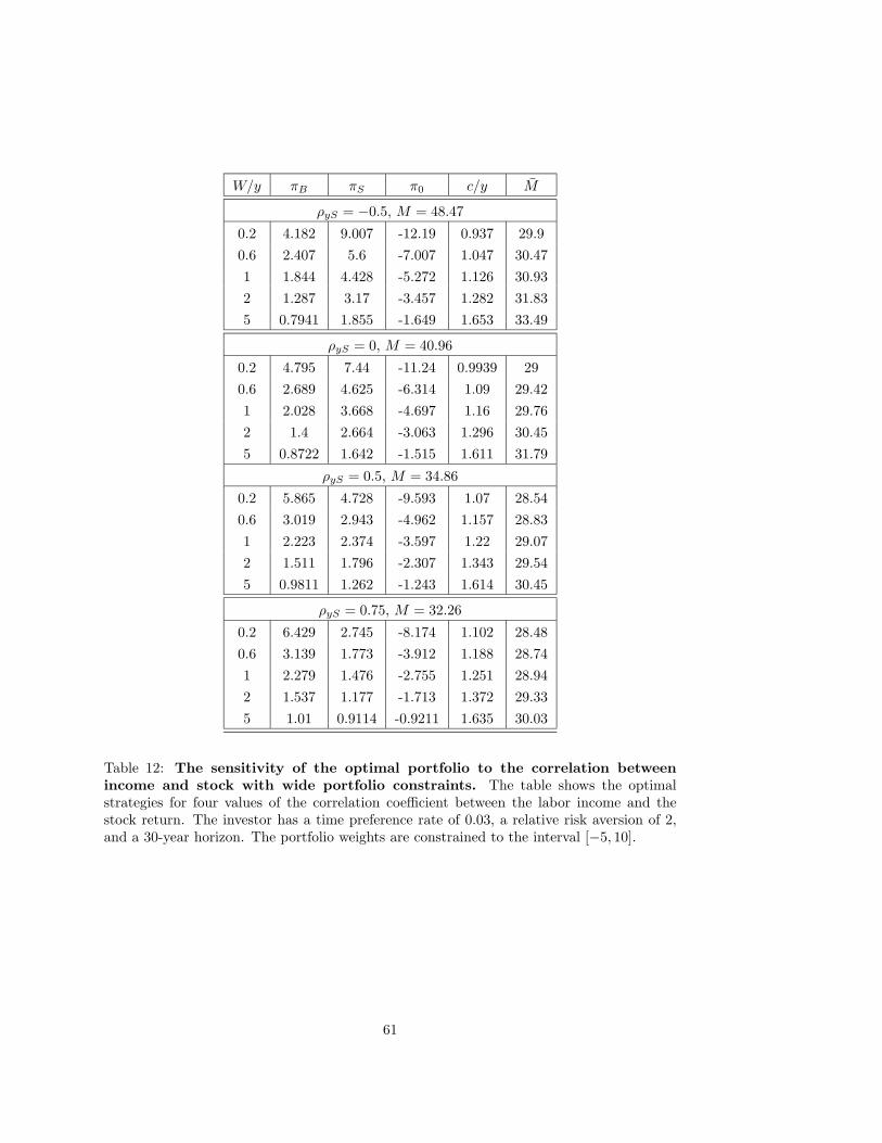
W/y πB πS π0 c/y M
ρyS = −0.5, M = 48.47
0.2 4.182 9.007 -12.19 0.937 29.9
0.6 2.407 5.6 -7.007 1.047 30.47
1 1.844 4.428 -5.272 1.126 30.93
2 1.287 3.17 -3.457 1.282 31.83
5 0.7941 1.855 -1.649 1.653 33.49
ρyS = 0, M = 40.96
0.2 4.795 7.44 -11.24 0.9939 29
0.6 2.689 4.625 -6.314 1.09 29.42
1 2.028 3.668 -4.697 1.16 29.76
2 1.4 2.664 -3.063 1.296 30.45
5 0.8722 1.642 -1.515 1.611 31.79
ρyS = 0.5, M = 34.86
0.2 5.865 4.728 -9.593 1.07 28.54
0.6 3.019 2.943 -4.962 1.157 28.83
1 2.223 2.374 -3.597 1.22 29.07
2 1.511 1.796 -2.307 1.343 29.54
5 0.9811 1.262 -1.243 1.614 30.45
ρyS = 0.75, M = 32.26
0.2 6.429 2.745 -8.174 1.102 28.48
0.6 3.139 1.773 -3.912 1.188 28.74
1 2.279 1.476 -2.755 1.251 28.94
2 1.537 1.177 -1.713 1.372 29.33
5 1.01 0.9114 -0.9211 1.635 30.03
Table 12: The sensitivity of the optimal portfolio to the correlation between
income and stock with wide portfolio constraints. The table shows the optimalstrategies for four values of the correlation coefficient between the labor income and thestock return. The investor has a time preference rate of 0.03, a relative risk aversion of 2,and a 30-year horizon. The portfolio weights are constrained to the interval [−5, 10].
61
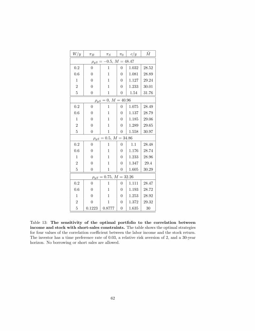
W/y πB πS π0 c/y M
ρyS = −0.5, M = 48.47
0.2 0 1 0 1.032 28.52
0.6 0 1 0 1.081 28.89
1 0 1 0 1.127 29.24
2 0 1 0 1.233 30.01
5 0 1 0 1.54 31.76
ρyS = 0, M = 40.96
0.2 0 1 0 1.075 28.49
0.6 0 1 0 1.137 28.79
1 0 1 0 1.185 29.06
2 0 1 0 1.289 29.65
5 0 1 0 1.558 30.97
ρyS = 0.5, M = 34.86
0.2 0 1 0 1.1 28.48
0.6 0 1 0 1.176 28.74
1 0 1 0 1.233 28.96
2 0 1 0 1.347 29.4
5 0 1 0 1.605 30.29
ρyS = 0.75, M = 32.26
0.2 0 1 0 1.111 28.47
0.6 0 1 0 1.193 28.72
1 0 1 0 1.253 28.92
2 0 1 0 1.372 29.32
5 0.1223 0.8777 0 1.635 30
Table 13: The sensitivity of the optimal portfolio to the correlation between
income and stock with short-sales constraints. The table shows the optimal strategiesfor four values of the correlation coefficient between the labor income and the stock return.The investor has a time preference rate of 0.03, a relative risk aversion of 2, and a 30-yearhorizon. No borrowing or short sales are allowed.
62
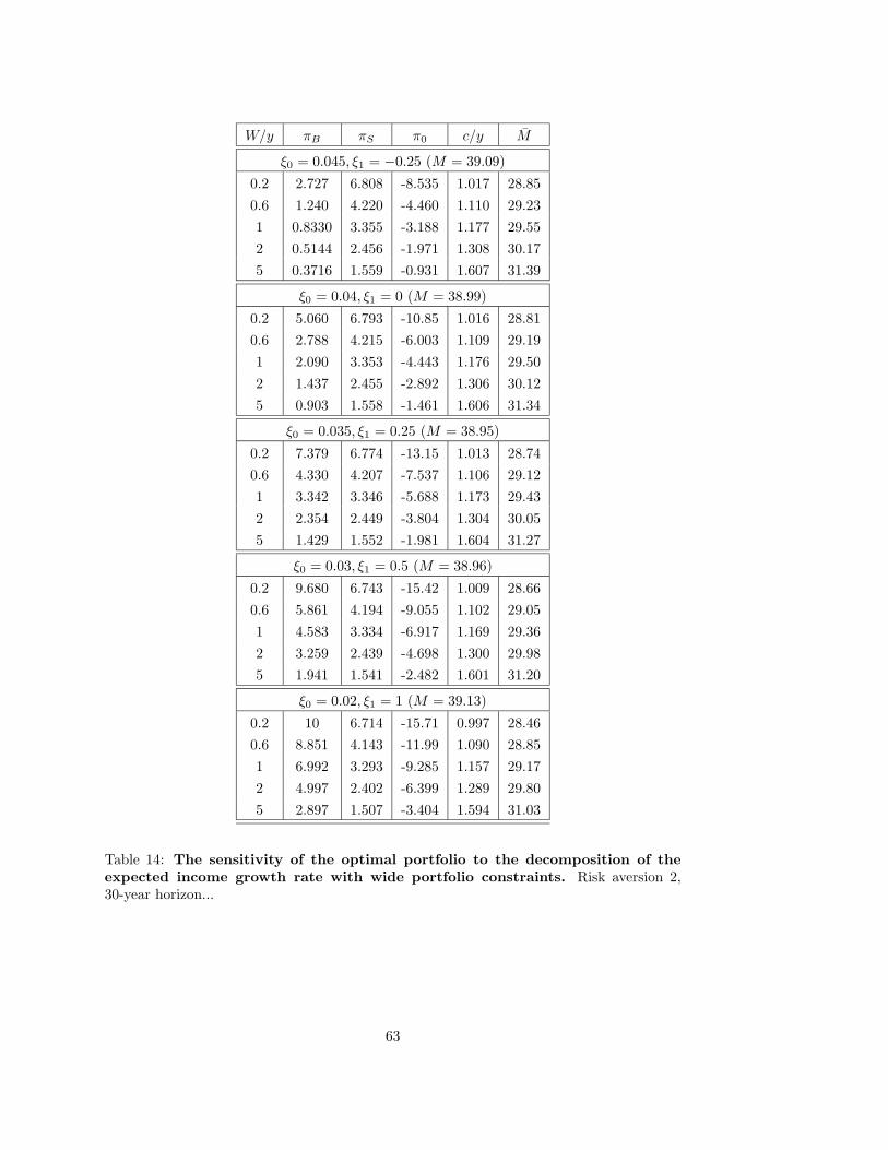
W/y πB πS π0 c/y M
ξ0 = 0.045, ξ1 = −0.25 (M = 39.09)
0.2 2.727 6.808 -8.535 1.017 28.85
0.6 1.240 4.220 -4.460 1.110 29.23
1 0.8330 3.355 -3.188 1.177 29.55
2 0.5144 2.456 -1.971 1.308 30.17
5 0.3716 1.559 -0.931 1.607 31.39
ξ0 = 0.04, ξ1 = 0 (M = 38.99)
0.2 5.060 6.793 -10.85 1.016 28.81
0.6 2.788 4.215 -6.003 1.109 29.19
1 2.090 3.353 -4.443 1.176 29.50
2 1.437 2.455 -2.892 1.306 30.12
5 0.903 1.558 -1.461 1.606 31.34
ξ0 = 0.035, ξ1 = 0.25 (M = 38.95)
0.2 7.379 6.774 -13.15 1.013 28.74
0.6 4.330 4.207 -7.537 1.106 29.12
1 3.342 3.346 -5.688 1.173 29.43
2 2.354 2.449 -3.804 1.304 30.05
5 1.429 1.552 -1.981 1.604 31.27
ξ0 = 0.03, ξ1 = 0.5 (M = 38.96)
0.2 9.680 6.743 -15.42 1.009 28.66
0.6 5.861 4.194 -9.055 1.102 29.05
1 4.583 3.334 -6.917 1.169 29.36
2 3.259 2.439 -4.698 1.300 29.98
5 1.941 1.541 -2.482 1.601 31.20
ξ0 = 0.02, ξ1 = 1 (M = 39.13)
0.2 10 6.714 -15.71 0.997 28.46
0.6 8.851 4.143 -11.99 1.090 28.85
1 6.992 3.293 -9.285 1.157 29.17
2 4.997 2.402 -6.399 1.289 29.80
5 2.897 1.507 -3.404 1.594 31.03
Table 14: The sensitivity of the optimal portfolio to the decomposition of the
expected income growth rate with wide portfolio constraints. Risk aversion 2,30-year horizon...
63
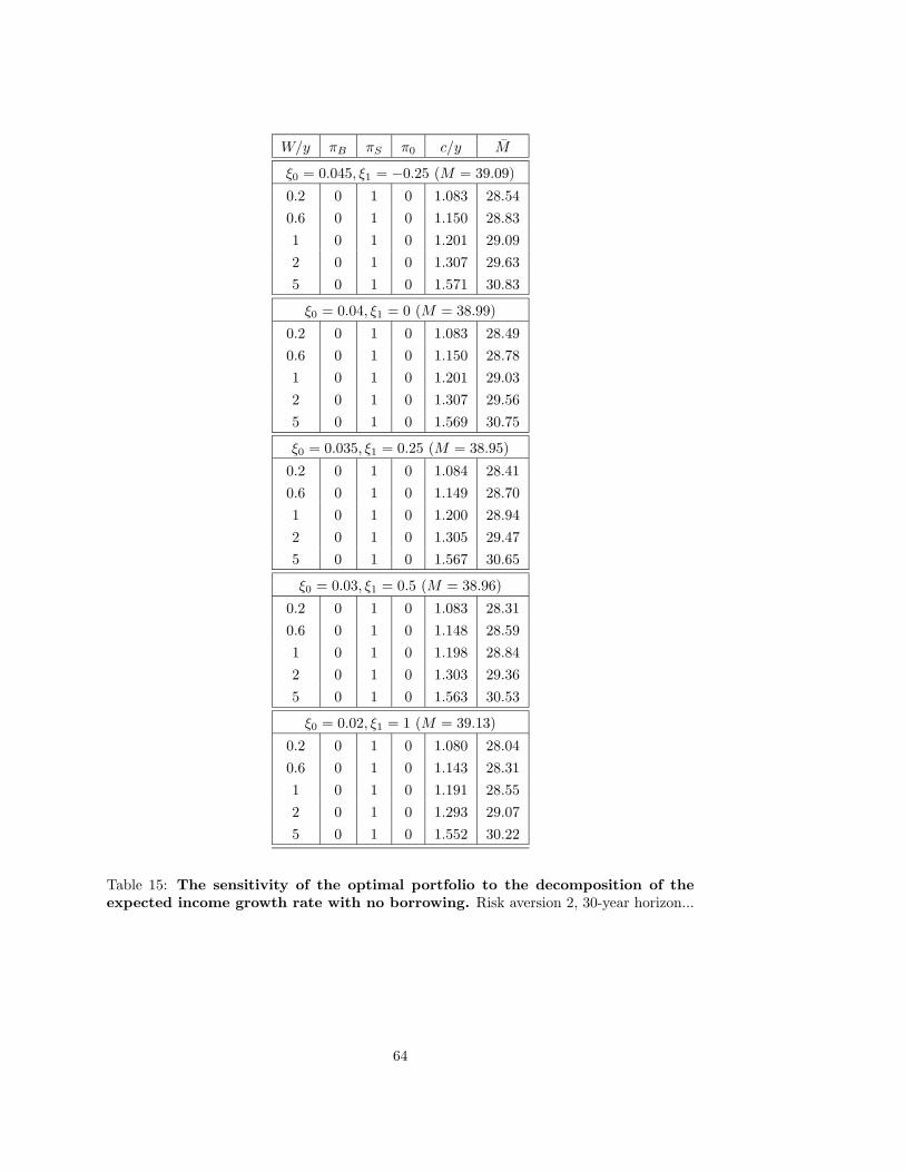
W/y πB πS π0 c/y M
ξ0 = 0.045, ξ1 = −0.25 (M = 39.09)
0.2 0 1 0 1.083 28.54
0.6 0 1 0 1.150 28.83
1 0 1 0 1.201 29.09
2 0 1 0 1.307 29.63
5 0 1 0 1.571 30.83
ξ0 = 0.04, ξ1 = 0 (M = 38.99)
0.2 0 1 0 1.083 28.49
0.6 0 1 0 1.150 28.78
1 0 1 0 1.201 29.03
2 0 1 0 1.307 29.56
5 0 1 0 1.569 30.75
ξ0 = 0.035, ξ1 = 0.25 (M = 38.95)
0.2 0 1 0 1.084 28.41
0.6 0 1 0 1.149 28.70
1 0 1 0 1.200 28.94
2 0 1 0 1.305 29.47
5 0 1 0 1.567 30.65
ξ0 = 0.03, ξ1 = 0.5 (M = 38.96)
0.2 0 1 0 1.083 28.31
0.6 0 1 0 1.148 28.59
1 0 1 0 1.198 28.84
2 0 1 0 1.303 29.36
5 0 1 0 1.563 30.53
ξ0 = 0.02, ξ1 = 1 (M = 39.13)
0.2 0 1 0 1.080 28.04
0.6 0 1 0 1.143 28.31
1 0 1 0 1.191 28.55
2 0 1 0 1.293 29.07
5 0 1 0 1.552 30.22
Table 15: The sensitivity of the optimal portfolio to the decomposition of the
expected income growth rate with no borrowing. Risk aversion 2, 30-year horizon...
64