1

DYNAMIC AND STOCHASTIC ROUTING

FOR

MULTIMODAL TRANSPORTATION SYSTEMS

S. Demeyer1,2, P. Audenaert1, M. Pickavet1, P. Demeester1

1 Dept. Of Information Technology (INTEC), Ghent University/IBBT,

Gaston Crommenlaan 8/201, B-9050 Ghent

2 Corresponding author: sofie.demeyer@intec.ugent.be

Abstract – We present a case study of a multimodal routing system that takes into account both

dynamic and stochastic travel time information. A multimodal network model is presented that

makes it possible to model the travel time information of each transportation mode differently.

This travel time information can either be static or dynamic, or either deterministic or

stochastic. Next to this, a Dijkstra-based routing algorithm is presented that deals with this

variety of travel time information in a uniform way. This research focuses on a practical

implementation of the system, which means that a number of assumptions were made, like, for

example, the modeling of the stochastic distributions, comparing these distributions, etc. A

tradeoff had to be made between the performance of the system and the accuracy of the results.

Experiments have shown that our system produces realistic routes in a short amount of time. It

is demonstrated that routing dynamically indeed results in a travel time gain in comparison to

routing statically. By making use of the additional stochastic travel time information even better

(i.e. faster) and more reliable routes can be calculated. Moreover, it is shown that routing in the

2

multimodal network may have its advantages over routing in a unimodal network, especially

during rush hours.

1. INTRODUCTION

With the evolvement of GPS systems, novel routing algorithms for transportation networks

emerge. In order to better predict the travel time of a route, dynamic travel time information

should be taken into account. Furthermore, more accurate travel time predictions can be made

by making use of stochastic information. This results in a route together with a stochastic

distribution of its travel time. With increasing traffic volumes, often resulting in congestion,

using multiple transportation modes (e.g. train, plane, ship, etc.) gains more interest. This

explains the appearance of multimodal routing algorithms that take into account multiple modes

of transportation to determine the best route between two locations (possibly using a sequence

of modes).

In this article, a multimodal dynamic and stochastic routing system is presented. This means that

it takes into account both the time-dependency and the uncertainty of the travel times.

Moreover, multiple modes of transportation are considered in order to find a better route

between an origin and a destination. To the best of our knowledge, routing systems

incorporating all these characteristics have never been realized before. Nevertheless, both

unimodal as multimodal systems exist that take into account either the time-dependency of the

travel time or the uncertainty. In section 1.1 we will review some of these systems and note the

differences and/or similarities with the system described in this article.

1.1. RELATED WORK The most common (early) routing systems presume the travel time data to be static, i.e.

independent of the time of the day. In this way, the well-known algorithm of Dijkstra [1] can be

applied in order to find the shortest (i.e., fastest) route between two locations. Since traffic is not

a static matter, more accurate travel times can be obtained by taking into account its dynamic

character, i.e., the (travel time) cost of a link is dependent on the time of the day this link is

3

traversed. To deal with dynamic travel times, the concept of time-based graphs (or dynamic

graph models) was introduced in which two major approaches can be distinguished: the time-

expanded and the time-dependent approach [2]. While in the time-expanded approach a node

exists for every event at a location and links represent time lapses between these events, in the

time-dependent approach each geographic location is represented by a single node and all

dynamic travel time information is stored in the links themselves. Due to the large number of

possible events in a road network, we opted for the time-dependent approach. Delling and

Wagner [3] give an overview of the current state of time-dependent route planning together

with a number of speed-up techniques. It includes some of the concepts we used in our research,

such as the modeling of dynamic travel times, the augmented algorithm of Dijkstra, etc. A

number of speedup techniques for dynamic shortest path routing, such as hierarchical routing

([4] and [5]) and bidirectional A* routing [6], have been proposed. Nevertheless, since we are

routing both dynamically and stochastically, these cannot be directly applied in our system.

Moreover, it has been shown that time-dependent shortest path computations indeed can

reduce the travel time significantly [7].

Road travel times are not only dynamic, but also contain an amount of uncertainty. One can

never be a hundred percent sure when to arrive at his/her destination, as the travel time is

influenced by random factors (individual driver’s behavior, weather conditions, traffic accidents,

etc.). We model the travel time by custom probability distributions and developed a stochastic

origin-destination shortest path algorithm. In the early days, some of the basic problems that

were encountered when developing stochastic shortest path algorithms, were tackled ([8], [9]

and [10]). Ji [11] presents three kinds of stochastic problems together with a genetic algorithm

and adapted linear programming methods to solve these problems. Unfortunately, these

algorithms have only been tested on small networks and are not scalable for very large (road)

networks. A promising dynamic stochastic algorithm is presented by Azaron and Kianfar [12].

They assume the travel times to have an exponential distribution, while we focus on the more

accurate custom distributions collected from actual travel time measurements. Li et al. [13] take

4

into account the stochastic properties of the travel time and study whether a long term

equilibrium exists. While we search mainly for the arrival time starting from a certain departure

time, they optimize the departure time for a preferred arrival time. Moreover, they do not assign

stochastic travel time distributions to the links, but look at a long term equilibrium. A

multicriteria A* shortest path algorithm was presented by Chen et al. [14]. They assume the

stochastic travel time of a link to be correlated with the travel times of the neighboring links.

Aside from the fact that this algorithm could only be tested on small networks, they do not take

into account the time-dependency of the travel times. Samaranayake et al. [15] provide a

theoretical basis for enabling tractable solutions to the arriving on time problem in a stochastic

environment and present a stochastic shortest path algorithm that performs well in road

networks. While we focus on a practical stochastic model, they approach it from a theoretical

point of view. Moreover, their main focus is on the non-time-dependent case.

By making use of multiple modes of transportation [16], travel times can be shortened. The main

issue in multimodal transportation systems is the modeling of the (different) information of the

different transport modes in a more or less uniform way. The most common solutions preserve

the network of each mode and interconnect these by the means of trans-shipment links, as we

described elsewhere [17], which is similar to the way this paper deals with multimodality. This

approach is denoted with the term hierarchical [18], alluding to the different sizes of the

transportation networks. Another multimodal network model is called a transfer graph [19]. It

consists of multiple components (typically one for each mode of transportation) with common

nodes where trans-shipments can take place. Moreover, when routing multimodally, other

objectives gain importance [20], such as number of transfers, transfer cost, waiting time, etc.

For more accurate routing, multicriteria algorithms should be used [21]. We opt to omit these

other objectives in this proof-of-concept and focus on the travel time. Nevertheless, we

incorporate the waiting time as part of the total travel time. The multimodal system presented

by Bielli et al. [22] resembles most to the system presented in this article. It incorporates

5

multiple modes of transportation and deals with the different travel time information of each of

these modes. Moreover, an origin-destination algorithm is presented to find the fastest path

between two locations. The main difference with the research presented here is that it does not

take into account the stochastic character of the travel time information.

In order to accurately predict the travel time between two locations, we made use of both time

table information and travel time data extracted from cellular networks [23]. This data was

provided by industrial companies within the IBBT ICON project MobiRoute [24].

1.2. OUTLINE In this article we present a case study of a practical industrial-strength multimodal routing

system, which efficiently calculates the routes taking into account the characteristics of the

travel time data, such as time-dependency and uncertainty. In the next section the time-

dependent network model is presented, in which a lot of attention is given to the cost modeling

as costs can either be static or dynamic and deterministic or stochastic. Subsequently (see

Section 3), a novel dynamic and stochastic shortest path algorithm is presented, which is based

on the algorithm of Dijkstra. In Section 4 it is shown that indeed a time gain can be realized by

routing dynamically, stochastically and multimodally. Moreover, when the stochastic travel time

information is used, more reliable paths are calculated. It is demonstrated that, by making use of

our data structures as presented in Section 2, these paths (with additional stochastic

information) can be calculated in an acceptable time. Then (see Section 5), we will have a glance

at the future version of this routing system with more transportation modes and additional

constraints. Finally, this paper is brought to an end with a number of conclusions. It should be

noted that the routing system presented here has been commercialized and a stripped down (bi-

modal) version for the Belgian network can be found online [25].

6

2. THE MULTIMODAL DYNAMIC NETWORK MODEL

In this section the multimodal network model is presented, in which multiple modes of

transportation are modeled. We opted to build one large network that contains a number of

mode-specific networks interconnected by trans-shipment links. Each of these mode-specific

networks is modeled in more or less the same way and the differences between the different

transportation modes are modeled in the cost objects that are attached to the links.

2.1. THE MULTIMODAL NETWORK The network model needs to be able to cope with dynamic costs. As mentioned in the

introduction, two major approaches exist to deal with this: the time-expanded network model

and the time-dependent network model. In the former every event (i.e., departure/arrival) at a

certain location is modeled as a node, which means that there are multiple nodes for one single

geographic location. In the time-dependent case, there is one single node for a geographic

location and all events are modeled in the links themselves.

We opted for the time-dependent network model, as the numbers of events can be immense,

especially for road networks. This would result in extremely large networks for the time-

expanded network model.

For every mode of transportation a network is built consisting of a node for every geographic

location that is of importance for this transport mode. If there exists a direct connection between

two geographic locations in this specific transportation mode, a link is constructed between the

corresponding nodes. In some cases, for example in the bus network, the number of changes

needs to be limited. One possible way to do this is by representing the station by one node and

adding dummy nodes for every service (for example a bus line) which stops at this location.

Getting off and on the bus can then be modeled as a link between the dummy and the station

node.

Once the networks are built for every mode of transportation, they are interconnected by trans-

shipment links. We opted to connect the nodes of every transportation mode to the closest

7

nodes in the densest network (usually this is the road network), as in this network almost all

geographic locations are reachable. Trans-shipments between two different (non-road)

transportation modes always pass through this (road) network, which is realistic as this usually

represents walking from one station to another. It should be noted that the walking network is

similar to the road network, but with walking travel times assigned to the links.

In the end, one large multimodal network is constructed, which consists of all mode-specific

networks connected together by trans-shipment links. Let us consider a multimodal transport

network with modes of transportation. The mode-specific network of mode then

can be represented by with a set of nodes and a set of links .

The trans-shipment links are represented by a set .

The complete multimodal network now is denoted by with and

.

2.2. COST MODELING As mentioned before, all mode-specific information is modeled in the cost objects. In this case

study, costs represent travel times. These costs can either be static or dynamic. If the time to

traverse a link is not dependent on the hour of the day, it is considered to be static and can be

represented as a single value. If, on the other hand, this cost is dynamic and thus dependent on

the hour of the day the specific link is taken, it can no longer be modeled as a single value, but as

a travel time function representing the travel time cost in function of the hour of the day.

Moreover, some of the travel time information has an amount of uncertainty attached to it. This

leads to stochastic travel time information. Instead of a single value, a time cost at a certain hour

of the day now is represented by a stochastic distribution. An overview of these different time

costs is given in Table 1, in which these two characteristics (static/dynamic and

deterministic/stochastic) are combined.

8

STATIC DYNAMIC

DETERMINISTIC Single value

Function of values

STOCHASTIC Single

distribution Function of

distributions

Table 1 Travel time costs

We will now discuss a practical example of each of these cases in more detail. Trans-shipment

costs are in most cases considered both static and deterministic. It takes always the same

amount of time and this time is independent of the hour of the day. These costs thus can be

represented by a single value.

In the railroad network (and all other networks which are bound to time tables), we consider

the costs to be dynamic and deterministic. The travel time, which consists of both a waiting time

in the station and a driving time, is dependent on the hour of the day, but considered to be

deterministic and thus independent of external factors. Time tables can easily be translated to a

travel time function as indicated in Figure 1 where the lowest points represent a train leaving

the station and the lines model the waiting in the station.

Figure 1 Travel time function in railroad network

9

Since waiting times are proportional to the hour of the day, this function can be represented by a

number of departure times, together with their corresponding driving time. Suppose the driving

time at departure time is , then the travel time at time between two known

departure times and ( ) can be calculated as follows:

A binary search algorithm can be applied to find the neighboring departure times. If memory

consumption is not an issue, a speedup can be realized by calculating the travel time for every

minute (i.e. the finest detail of the time table) and storing this in an array which then can easily

be accessed by translating the specific hour of the day to the corresponding index. This leads to

faster travel time calculations, but has a major impact on the memory consumption. Since the

networks that are used in our proof-of-concept system are relatively small, we can make use of

these memory-intensive arrays to store the travel time information, with the advantage of fast

lookup operations.

In an underground network, subway trains leave the station every minutes, but are not bound

to a specific time table. This introduces an amount of uncertainty which leads to a stochastic and

static (supposed day and night are equal) time cost. Suppose for example, a subway train leaves

every 6 minutes and driving to the next station takes 2 minutes, then the travel time of this link

lies somewhere between 2 and 8 minutes depending on the time one arrives in the subway

station. We will make use of a cumulative distribution which contains for each probability the

maximum travel time. In the example we have a 100% chance to travel less or equal than 8

minutes, while we have 50% chance of travelling less than 5 minutes. In order to both save

memory and simplify the calculations, we will represent a stochastic distribution by values,

corresponding to predefined percentiles. The -th percentile of a stochastic distribution is the

value that is higher than of all values of the distribution. This number results in a trade-off

10

between accuracy and performance. The more percentiles, the more accurate the results, but the

more storage space is needed.

In a road network, travel time costs are both dynamic and stochastic. Due to possible traffic jams

the travel time in a road network is dependent on the hour of the day. Moreover, external factors

(for example traffic accidents) are the cause that one can never be sure when to arrive precisely

at the destination. The dynamic and stochastic travel time costs are modeled as a function of

distributions. In our use case, travel time data was collected for every quarter of an hour during

multiple (similar) days. Stochastic distributions are constructed from this data for each quarter

of an hour for each day of the week (i.e. Monday, Tuesday, …). For the times in between these

quarters, linear interpolation is used between the corresponding percentiles. The x-th percentile

of the travel time distribution at time between two timestamps (i.e. quarters) and

( ) then can be calculated as follows:

A more accurate travel time function can be obtained by adding more timestamps, at the cost of

more intensive memory usage.

3. THE ROUTING ALGORITHM

As indicated in the previous section, a multimodal graph consists of a set of nodes and a set of

links , which consists of links specific to a certain transport mode and trans-shipment links.

Each of these links has assigned to it a travel cost, which can be a single value

(static/deterministic), a function of values (dynamic/deterministic), a distribution

(static/stochastic) or a function of distributions (dynamic/stochastic).

In this section, we present a shortest path algorithm that is adjusted to deal with both dynamic

and stochastic travel time information. As both static and deterministic information can easily be

11

translated to dynamic and stochastic functions respectively, we will develop an algorithm which

assumes all travel time information to be dynamic and stochastic.

The problem that is addressed here can be described as follows. Given an origin and destination

node together with a departure time, find the path between the origin and the destination that

has the ‘smallest’ distribution of the arrival time, according to a comparison measure that will be

defined further on. The network, in which the routing happens, contains multiple modes of

transportation and the travel time costs can either be static or dynamic, and deterministic or

stochastic.

The algorithm presented here is based on the algorithm of Dijkstra [1], a label-setting algorithm

with labels representing the shortest distance between the origin and the specific node. During

initialization the label of the origin node is set to zero and all other labels are set to infinity. The

set contains all (non-permanent) nodes whose labels have been updated by the algorithm. In

every iteration the node with the lowest label is removed from and made permanent. Then, all

labels of the neighboring nodes are updated. More specifically, if the sum of the label of the

investigated (permanent) node and of the link cost is smaller than the previous label of the

neighboring node, then the label is changed to this sum. This process is repeated until the

destination node has been made permanent. The algorithm of Dijkstra requires all link cost to be

non-negative values, which is the case as we are working with travel times here.

The algorithm described above needs to be altered in two ways. Firstly, the dynamic character of

the links costs needs to be taken into account when determining the travel time on a link.

Secondly, labels are no longer single values but distributions. We need to define how to combine

and compare stochastic distributions with each other.

In order to make this algorithm dynamic, some small adaptations are needed. Labels now

represent the earliest time at which one can arrive in a specific node starting at the origin node

at a specific departure time. In the initialization phase the origin label is set to this departure

time. Furthermore, the travel time of a link is dependent on the time at which this link is

12

traversed. For a link this time is equal to the label of the start node . The value of a

tentative new label can then be calculated as follows:

When the algorithm is finished, the label of the destination node represents the earliest arrival

time, starting at a predefined departure time in the origin node.

Making this algorithm stochastic introduces new challenges. Labels are no longer single values,

but probabilistic distributions of travel times, represented by a number of percentiles. Two

operations need to be defined: comparing labels and updating labels. Deciding which of two

labels is the ‘best’ is no unambiguous process. We opted to compare a single percentile. In most

cases the 50% percentile suffices, but if the user is interested in a more certain solution a higher

percentile can be used, such as the 90% percentile. A more accurate comparison would involve

all percentiles and applying a multi-objective algorithm, but this would require a higher amount

of computing power.

To define the sum of two labels we investigate two extreme cases, namely one in which the

distributions of the links are completely correlated and one in which they are completely

uncorrelated (and stochastically independent). While in the former the pointwise sum can be

used, the latter needs the convolution product to combine two labels. In the stochastic case, the

label of node can be represented as an array of percentiles , (note: in the

remainder of this article we will omit the boundaries of and use square brackets to denote an

array over index ). The pointwise sum of two labels and then can be defined

as:

Calculating the convolution product is more complex. In calculus, the convolution product of two

functions f and g can be defined as

13

When the distributions are represented as a number of percentiles, the convolution sum of two

labels and can be determined as follows. Calculate for each and :

. The requested percentiles then can be extracted from the distribution of

these values. It should be noted that determining percentiles in large arrays can be sped up

by making use of order statistics [26].

In reality, some of the links are correlated with each other, while others are not. For example,

two consecutive sections on a highway are closely correlated. A traffic jam in one of the sections

increases the chance of a traffic jam in the other section. On the other hand, a section on the

highway has nearly no correlation with a small road besides it. As determining all correlations

between all links of the network and then combining the costs of these links appropriately is

very burdensome, we will work with these two extreme cases. The user then can decide how

much he wants to tempt his fate making use of these calculated boundaries.

Below, the pseudo code of the algorithm as described above is given. It should be noted that

represents a constant distribution with value .

[1] l(o) = [departure_time]

[2] l(v) = [∞], v≠o

[3] P = {o}

[4] while( l(d)=[∞] || d ∈ P){

[5] x = remove_smallest(P)

[6] for(y: neighbor(x)){

[7] new_distribution = l(x) ∎ translate(cost((x,y), l(x)))

[8] if(new_distribution < l(y)){

[9] l(y) = new_distribution

14

[10] P = P U {y}

[11] }

[12] }

[13] }

The first three lines are the initialization phase. The label of the origin node is set to a constant

distribution of the departure time (line [1]), while all other labels are set to the infinity

distribution (line [2]). Subsequently, the temporary set is initialized with a singleton containing

the origin node (line[3]). As long as the destination node is not permanent, i.e., as long as its

label is the infinity distribution or it is an element of the temporary set (line [4]), the following

steps are executed. Firstly, the node with the smallest label is removed from the temporary set

(line [5]). For each neighbor or this node, a new tentative label is determined by combining the

label of with the dynamic and stochastic cost of the link between and (line [7]). If the cost

of the link is static or deterministic, it is translated to a dynamic and stochastic one. We assume

the distributions to be either completely correlated or completely uncorrelated, as described

above. The operator ∎ can thus either represent a pointwise sum or a convolution product.

When this tentative label appears to be smaller (w.r.t. the comparison operator as described

above) than the previous label of , it is changed and the temporary set is updated (line[8] to

line[10]).

4. RESULTS

In this section it is shown that indeed a travel time gain can be realized by routing dynamically

(in comparison to routing statically), stochastically (in comparison to deterministically) and

multimodally (in comparison to unimodally). Moreover, when routing stochastically, additional

information about the travel time is provided to the user. After a general description of the setup

of the system and the experiments (see Section 4.1), some light is shed on the execution times of

the different algorithms (see Section 4.2). Subsequently, we will investigate the deterministic

case and show how better (i.e. faster) routes can be calculated by making use of dynamic

15

information (see Section 4.3). Section 4.4 deals with the core issue of our research, namely

stochastic routing. It will be demonstrated that, indeed, by making use of additional stochastic

information, more reliable routes can be calculated. Here, we will examine the two extreme

cases, namely assuming all links are completely correlated and assuming all links are completely

uncorrelated. In Section 4.5, we will have a look at multimodal routing in comparison with

unimodal routing. It will be shown that making use of multiple modes of transportation may

have its advantages in particular cases, especially during rush hours.

4.1. GENERAL DESCRIPTIONS OF SETUP

The routing system as described in this article was implemented in Java (version 1.6.0-18) on a

machine with the following specifications: Intel ® Core TM 2 Duo CPU P8600, 2.40 GHz and 4 GB

of RAM.

Currently, the system contains only two modes of transportation, namely road and railroad, but

we are gathering data of the other transport modes to further expand the network. For the

experiments we made use of a bimodal Belgian network (as for this network we have very

detailed travel time information at our disposal) composed of a road network of 53010 nodes

and 96286 links and a railroad network of 551 nodes and 1716 links. For each train station three

trans-shipment links were added connecting it to the road network.

Stochastic distributions, represented as 5 percentiles (i.e. the 10%, 30%, 50%, 70% and 90%

percentile) were calculated for the road links based on historical measurements of travel times.

Railroad time tables were analyzed and translated to the data structure as presented in section

2. We opted for an array with a travel time for every minute of the day, as there is sufficient

memory available for these networks. While for the railroad network a dynamic granularity of 1

minute was used, the road network employs a granularity of 15 minutes, due to the data

restrictions of the measurements. Interpolation, as shown in section 2, is applied for the times in

between timestamps.

16

In the experiments the different algorithms are compared to one another. To compare the

(travel time) costs of the resulting paths, a difference measure was defined. The amount of

difference ( ), in percentage, of the cost of the path calculated by algorithm (2) compared to the

cost of the path calculated by algorithm (1) is

Both the average and the maximum values of this parameter will be reported.

All the experiments of the following subsections were executed on the multimodal network as

described above, unless explicitly stated otherwise.

4.2. CALCULATION TIME

First and foremost, we investigated the performance of the algorithms. Table 2 shows the

average calculation times (in ms) of all algorithms that were used during the experiments.

The static deterministic algorithm is in fact the standard Dijkstra algorithm in a network where

all travel time costs are assumed to be constant. When the link costs are dynamic travel times,

we opted to use the values of a quiet timeslot (i.e. a timeslot outside of the rush hours). This

represents driving when there is not much traffic, such as driving at night. When the travel time

information is stochastic, the median values (i.e. 50% percentile) are used.

The dynamic deterministic algorithm takes into account the dynamic travel time information but

still assumes the travel times to be single values. For the links with stochastic distributions

assigned to them, the median values were used.

The static stochastic algorithm makes use of a single stochastic distribution for each link. When

the travel times are dynamic stochastic, again we opted to use a distribution of a timeslot in the

night.

17

In the dynamic stochastic algorithm, all available travel time information was used to calculate

the best (fastest) routes. The stochastic algorithms were executed for two extreme cases, namely

assuming that all links are completely correlated (using the pointwise sum) and assuming that

they are completely uncorrelated (using the convolution product).

Calculation Time (ms)

static deterministic 10.7 dynamic deterministic 20.9 static stochastic (correlated) 30.7 static stochastic (uncorrelated) 37.6 dynamic stochastic (correlated) 43.3 dynamic stochastic (uncorrelated) 48.9

Table 2. Average calculation times of the different algorithms

The results of Table 2 are averages of 10 000 shortest path calculations with randomly chosen

origin-destination pairs and random departure times. It can be seen that taking into account the

dynamic information slightly slows down the calculations (static vs. dynamic). Moreover, for the

stochastic algorithms, assuming the links are completely uncorrelated consumes more

calculation time that assuming that they are completely correlated. This is as expected as the

convolution product is a more complex operation than the pointwise sum.

The results show that for these algorithms the two most crucial operations are determining the

travel time of a link at the time this link is traversed and combining this travel time information.

While in the static deterministic case the constant cost values of the links can just be added up,

in the dynamic cases the exact travel time needs to be determined by making use of the arrival

time in the start node of the link in question. For the stochastic algorithms combining the

distributions even adds more computational complexity to the problem.

These calculation times are indeed acceptable, as they stay below 50 ms while providing better

(i.e. faster) and more reliable routes.

18

4.3. DETERMINISTIC ROUTING: DYNAMIC VS. STATIC ROUTES

In this subsection, it will be demonstrated how better (i.e. faster) routes can be calculated by

making use of the dynamic travel time information. We will start with a small example to show

that routing dynamically indeed has its advantages. In the unimodal road network a route was

calculated from Ghent to Liège for different departure times. This route passes through Brussels

which is a known bottleneck of the Belgian road network. Parts of these routes, namely those

around Brussels, are depicted in Figure 2, when leaving at 6 am, 7 am and 8 am. It can be seen

that, during rush hour, the ring road around Brussels is avoided. At 7 am, the highway before

Brussels is left earlier in order to avoid the first part of the ring way. At 8 am, a road going

through the center of Brussels proves to be faster than waiting in the traffic jams on the ring

road.

Figure 2 Dynamic Routes in Belgian Road Network

Table 3 shows the actual travel time gain realized by the static deterministic algorithm in

comparison to the dynamic deterministic algorithm. For this, 10 000 paths were calculated

between random origin-destination pairs at a random departure time. Subsequently, both the

dynamic deterministic and the dynamic stochastic costs of the resulting paths were calculated.

For this, the actual travel time costs were removed from the paths and recalculated assuming

that all links of the paths are dynamic deterministic and dynamic stochastic respectively. The

differences between these travel time costs (i.e. the recalculated costs of the paths calculated by

both algorithms) are reported in the table.

19

travel time cost average Δ (%) maximum Δ (%)

dynamic deterministic

14.25 56.96

10% 30% 50% 70% 90% 10% 30% 50% 70% 90%

dynamic stochastic (correlated)

-2.59 -0.42 1.19 3.24 3.68 25.92 32.09 35.61 42.75 49.30

dynamic stochastic (uncorrelated)

0.78 1.27 1.66 2.04 2.35 34.31 34.53 34.65 35.91 36.93

Table 3 Comparison of the travel times of the paths calculated by the static deterministic algorithm (1)

and the dynamic deterministic algorithm (2)

First of all, the dynamic deterministic travel time costs were compared. The paths calculated by

the dynamic deterministic algorithm are on average 14.25% shorter than the paths of the static

deterministic algorithm, with a maximum value of 56.96%. This proves that, indeed, making use

of the dynamic travel time information in the routing algorithm has its benefits. In 85.12% of the

cases, a shorter route has been found by the dynamic deterministic algorithm.

Next, we looked at the stochastic costs, for both extreme cases, and compared the corresponding

percentile values with one another. Despite of the fact that the average values are relatively

small, if we look at the maximum values still a remarkable travel time gain can be realized by

routing dynamically instead of statically. Moreover, the amount of difference between the two

algorithms is higher for the higher percentile values. This means that for users who want more

reliability routing dynamically really pays off. For the lower percentiles, routing dynamically is

on average even slightly worse than routing statically assuming the links are completely

correlated. If we compare the case in which is assumed that all links are completely correlated

20

(using pointwise sum) and the case in which they are assumed to be completely uncorrelated

(using convolution product), we see that the difference between the lowest and the higher

percentiles is larger when using the pointwise sum. This is as expected, since in the pointwise

sum, the extreme values are combined with each other, while the convolution product takes into

account all values of the distributions smoothing out the extreme values.

4.4. STOCHASTIC ROUTING

This subsection deals with stochastic routing. We will demonstrate that by making use of the

additional stochastic travel time information, more intelligent routes can be calculated. After an

example that illustrates the difference between the two extreme cases (i.e. the links are

completely correlated vs. completely uncorrelated), two aspects will be investigated. First we

will compare the static stochastic algorithm with the dynamic stochastic algorithm and report on

the travel time gain that can be realized by routing dynamically. Subsequently, a comparison is

made between the dynamic deterministic algorithm and the dynamic stochastic algorithm to

illustrate the strength of using the additional stochastic information to come to more intelligent

routes.

With respect to combining stochastic distributions, two extreme cases were investigated:

completely correlated links (with the pointwise sum) and completely uncorrelated links (with

the convolution product). In Figure 3 an example is given of a day overview for one specific path

in both scenarios. The dynamic stochastic shortest route was calculated for each time of the day

in the unimodal (road) network and the resulting percentiles were plotted. Here distributions

were compared w.r.t. their 50% percentiles.

The rush hours can be readily observed, namely a major one in the morning (7 am-9 am) and a

smaller one in the evening (4 pm-6 pm). Moreover, it should be noticed that the 50% percentile

values are similar with only differences of a couple of seconds. The main difference between the

two calculation methods lies in the other percentiles. While the standard deviation in the

uncorrelated case is small, the percentiles of the correlated case are more scattered. This can be

21

explained intuitively as the convolution product takes into account all values of the distributions,

resulting in extreme values being weakened by the others. In the completely correlated case

(pointwise sum) a high probability of congested traffic on one link of the network results in a

higher probability on all other links following this link. Extreme percentile values have a direct

influence on the corresponding percentile of the resulting distribution.

As mentioned before, the percentiles of the actual distribution lie somewhere between these two

extremes. This means that for the percentiles under the 50% percentiles (which is used here for

comparison) the uncorrelated case is an upper bound and the correlated case a lower bound.

The opposite is true for the percentiles above the 50% percentile. If the user wants more

certainty of its arrival time, i.e. he wants to be sure to be at his destination at the latest at a

certain chosen time, the 90% percentile can be used to compare labels. In this case the pointwise

sum calculations always serve as a lower bound.

In the remainder of this section stochastic distributions will be compared by comparing their

90% percentile values.

22

Figure 3 Stochastic Day Overview

Top: correlated links (pointwise sum) – Bottom: uncorrelated links (convolution product)

4.4.1. Static Stochastic vs. Dynamic Stochastic

Table 4 shows the average and maximum amount of difference between the travel times of the

paths calculated by the static stochastic algorithm and the dynamic stochastic algorithm for the

two extreme cases. These values were calculated from 10 000 shortest path calculations

between random origins and destinations at random departure times. Similar to the statements

made in section 4.3, indeed a travel time gain can be realized by making use of the dynamic

character of the travel time information. Despite the relatively low average values, the maximum

travel time gain is noteworthy. To compare labels with one another, we made use of the 90%

23

percentiles, so the resulting paths are optimized with respect to this percentile. The results show

that indeed the highest travel time gains are realized for this percentile.

links are … average Δ (%) maximum Δ (%)

10% 30% 50% 70% 90% 10% 30% 50% 70% 90%

completely correlated

2.20 2.31 2.14 3.81 7.29 35.90 36.02 37.16 39.44 50.39

completely uncorrelated

1.23 1.59 1.85 2.04 2.31 33.17 34.44 35.82 36.82 37.72

Table 4 Comparison of the travel times of the paths calculated by the static stochastic algorithm (1)

and the dynamic stochastic algorithm (2)

Next we looked at the amount of better paths (w.r.t. the 90% percentile values of the

distributions) that were calculated by routing dynamically. In the situation that all links are

assumed to be completely correlated, in 81.82% of the cases a better path is found, while in the

other situation (all links are completely uncorrelated), this comes down to 65.06% of the cases.

This proves that it is worth routing dynamically when the information is available.

In conclusion, for users who are interested in reliable routes (making use of the 90%

percentiles), by routing dynamically instead of statically a travel time gain of up to 50% can be

realized in the case all links are correlated, and nearly 38% in the case the links are completely

uncorrelated.

4.4.2. Dynamic Deterministic vs. Dynamic Stochastic

In this section we will investigate the advantages of using the stochastic travel time information

in the algorithm and compare the dynamic deterministic algorithm with the dynamic stochastic

one. Again the shortest paths were calculated for 10 000 randomly chosen origin-destination

pairs at random departure times. The stochastic travel time was then calculated for the resulting

shortest paths and all percentile values were compared to one another. The average and

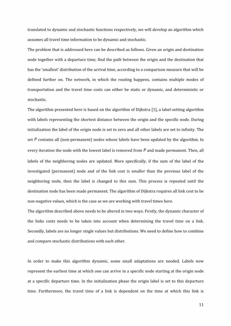
maximum amounts of difference are shown in Table 5.

24

links are … average Δ (%) maximum Δ (%)

10% 30% 50% 70% 90% 10% 30% 50% 70% 90%

completely correlated

-1.36 -0.97 -0.71 -0.75 2.69 22.78 18.94 14.27 18.36 81.32

completely uncorrelated

0.88 0.80 0.74 0.66 0.75 19.32 15.31 13.77 13.77 51.03

Table 5 Comparison of the travel times of the paths calculated by the dynamic deterministic algorithm (1)

and the dynamic stochastic algorithm (2)

The average values of

Table 5 Table 5 are small, meaning that on average not that much travel time gain can be

realized by routing stochastically. In the case that all links are assumed to be correlated, for the

lower percentiles the paths calculated by the stochastic algorithm are even worse than those

calculated by the deterministic algorithm. However, the paths calculated by the stochastic

algorithm are more reliable than those calculated by the deterministic algorithm. Looking at the

90% percentiles (for which these paths were optimized, i.e. minimized), we see that for this

percentile indeed a travel time gain is realized by the stochastic algorithm. This means that more

reliable paths are calculated.

If we look at the maximum amount of difference of the 90% percentile values, we see that travel

time gains can be realized of up to 81.32% and 51.03% for the correlated and the uncorrelated

case respectively, which is quite remarkable. Users who are interested in reliable routes can

really benefit from routing stochastically.

Subsequently, for each origin-destination pair the 90% percentiles of the travel time

distributions of the paths found by both algorithms were compared with each other. When it is

assumed that all links are uncorrelated, 53.30% of the paths are actually better, while only

12.75% of the paths are worse. For the case that all links are correlated, these numbers are

37.61% and 33.42% respectively. As more reliable routes are produced, routing stochastically

indeed is valuable. So, in 87.25% (completely uncorrelated) and 66.57% (completely correlated)

25

of the cases the paths are as well as or better than the paths calculated by the deterministic

algorithm. Moreover, the resulting routes are more reliable. This means that making use of the

stochastic travel time information when determining the shortest path, indeed is valuable.

4.5. MULTIMODAL VS. UNIMODAL ROUTING

The system presented here is multimodal, which means that both roads and railroads are taken

into account. In this section we will determine whether travelling multimodally indeed has

advantages (with respect to the travel time) over travelling unimodally. We start with a small

example, which is similar to the example of section 4.3, as it also concerns the bottleneck around

Brussels in the Belgian road network. In Figure 4 the multimodal routes between Leuven (on the

right) and Ghent (on the left) are depicted for different departure times. These routes were

calculated with the dynamic deterministic algorithm. While in the example in section 4.3 the

traffic jams around Brussels were avoided by taking other routes in the road network, here the

traffic jams are avoided by making use of another mode of transportation, namely railroads.

Outside the rush hour, for example at 6 am, the road is chosen to be the best mode of

transportation. Nevertheless, when traffic is jammed around Brussels (in the case of leaving at

7:30 am) the train becomes more favorable. Combinations of both transport modes are also

possible. For example, at 7 am the best route is the one leaving by car in Leuven and taking the

train in Brussels to continue to Ghent.

26

Figure 4 Multimodal Routes (Leuven-Ghent)

red = road - blue = railroad

Next, a more systematic comparison was performed. For this, routes were calculated between 10

000 random origin-destination pairs in both the unimodal (road) and the multimodal (road-

railroad) network (making use of the dynamic stochastic algorithm). As the previous example

shows that during rush hours the multimodal network might be more favorable than outside

these rush hours, these two cases were examined separately, namely starting at 7:30 am (during

the rush hour) and departing at 2 pm (outside of the rush hour). Results are shown in Table 6.

27

links are … average Δ (%) maximum Δ (%)

DURING RUSH HOUR (7:30 am)

10% 30% 50% 70% 90% 10% 30% 50% 70% 90%

completely correlated -1.32 -0.41 -0.09 1.50 1.69 38.37 40.16 39.83 41.73 41.89

completely uncorrelated

0.72 0.79 0.83 0.89 0.89 41.31 41.28 41.02 41.51 41.86

OUTSIDE RUSH HOUR (2 pm)

10% 30% 50% 70% 90% 10% 30% 50% 70% 90%

completely correlated

-0.23 -0.03 0.02 0.12 0.31 4.20 6.33 7.14 19.77 24.33

completely uncorrelated

0.16 0.17 0.18 0.19 0.19 14.01 14.19 14.67 15.33 15.88

Table 6 Comparison of the travel times of the paths in the unimodal network (1)

and the multimodal network (2)

The average travel time gain by using the multimodal network is almost negligible outside of the

rush hours. Moreover, in approximately 5% of the cases (5.58% and 4.46% for the completely

uncorrelated and correlated case respectively) a better path is found in the multimodal network.

During these hours, taking the car is in most cases more advantageous than using multiple

modes of transportation. It should be noted that, if a unimodal path is the best option to get from

the origin to the destination, this path will be returned by the algorithm, even when routing in a

multimodal network. When traveling during the rush hours, multimodal transportation may

result in travel time gains of up to more than 40%. Moreover, during the rush hours in

approximately 15% of the cases (14.13% and 14.87% for the completely uncorrelated and

correlated case respectively) a better path (according to the 90% percentiles) is found in the

multimodal network.

All multimodal paths were inspected more closely and it was observed that the origin and/or

destination of these routes are situated close to train stations, which is as expected. If the origin

and the destination are situated far from train station, a multimodal route would consist of a

rather long path from the origin to the ‘closest’ train station, followed by a train ride, followed by

28

a rather long path from the last train station to the destination. In most cases, this cannot

compete with a direct route by car.

Next, we investigated for which origin-destination pairs a better route was found in the

multimodal network. More specifically, it is determined whether routing multimodally is more

rewarding for short range routes or for long range routes. For this, 10 000 paths (with random

origin-destination pairs) were calculated in both the unimodal and the multimodal network and

both during and outside the rush hour. In this experiment the dynamic stochastic algorithm was

used. These paths were ordered according to their Dijkstra-rank (defined as the number of

nodes that have been made permanent when the algorithm finishes) and divided into 10

categories. For each of these categories the percentage of paths that are multimodal (i.e. paths

that are better in the multimodal network compared to unimodal ones) was then calculated.

Results are shown in Figure 5. Here we assumed that all links are completely correlated. Similar

results are obtained when all links are uncorrelated. It is clear that routing multimodally has

more advantages for long range paths, and during the rush hours. When the origin and the

destination are situated further apart (i.e. a higher Dijkstra-rank), the percentage of multimodal

paths increases steadily. Outside the rush hour, this phenomenon is not that prominent. Here,

the main promoter for multimodal transportation is whether the origin and the destination are

situated close to train stations.

29

Figure 5. Percentage of multimodal paths in function of the Dijkstra-rank.

As the travel time gain of multimodal routing over unimodal routing differs depending on the

departure time, we want to investigate how this evolves during the day. For this, the fastest

route was calculated between one origin (Ghent) and one destination (Leuven) for a number of

different departure times (with the dynamic stochastic algorithm, assuming all links are

completely uncorrelated). The 90% percentile values for these different departure times are

depicted in Figure 6. When the travel time in the multimodal network is equal to that in the

unimodal network, this means that the route in the multimodal network is in fact unimodal as no

travel time gain can be realized by multimodal routing. Again, it is seen that routing

multimodally is most advantageous during the rush hours. So, for commuters, taking the train is

a good alternative. The irregular shape of the multimodal travel time function is due to the time

table restrictions in the train network. The travel time is higher when users have to wait longer

in the stations.

30

Figure 6. Comparison of travel times in unimodal and multimodal networks (day overview)

In conclusion, while in most cases the road network seems to be more rewarding, multimodal

transportation (in this case study: taking the train) proves to be a good alternative to travel

between major cities (i.e. close to train stations) and long distances at rush hour.

5. FUTURE WORK

As mentioned previously, a proof-of-concept system has been built making use of both road and

railroad travel time data. In the future we would like to incorporate other transportation modes

as well, like bus transport, subways, trams, etc. This was not possible at this moment, as we are

still gathering data of these transport modes. The travel time costs of most of these public

transportation modes could be modeled similarly to the railroad travel times as presented in

this article with a similar translation of the time table information.

Furthermore, better predictions of the trans-shipment travel times could be made by making use

of additional information. For example, information about the parking possibilities around

stations could help with more accurate predictions of the trans-shipment costs, as the trans-

shipment cost in the current system is a fixed (slow walking) travel time. Moreover, in our proof-

of-concept system, trans-shipment between the railroad and road network is always possible,

31

even when no car is available. It is supposed that at each station a taxi or car rental service is

present. Additional information about these services could help us define better constraints on

the trans-shipment possibilities. Additionally, if other public transport mode information would

be available, a trans-shipment to for example bus transport can be a valuable when arriving in a

station where no car is available.

The perfect multimodal system would have access to all information about all modes of

transportation and make more clever routing decisions making use of the additional (trans-

shipment) constraints. This would only have a minor impact on the shortest path algorithm

presented in this article as constraints can be stored in the labels. Then, in each iteration of the

algorithm, only the neighbors which are accessible, with respect to the constraints, are updated.

In the ideal case, the system should be able to route worldwide. To realize this, the algorithm

presented in this article needs to be accelerated. We aim at investigating a promising technique

to speed up shortest path routing algorithms, namely by making use of a hierarchical approach

(for example [27], [28] and [29]). One of the most promising approaches here are contraction

hierarchies [28]. At this moment, research has been done to construct time-dependent

contraction hierarchies [30], but no ready-made solution exists to deal with stochastic

information.

6. CONCLUSION

In this article we presented a case study of a novel practical multimodal routing system. Next to

the dynamic travel times, additional information about the (un)certainty of the results is

calculated. A lot of attention was given to the design of efficient data structures to store the

needed travel time information. Making use of these data structures an algorithm was developed

to calculate the shortest path between two locations, both dynamically and stochastically.

Experiments have shown that by routing dynamically, stochastically and multimodally indeed a

travel time gain can be realized by avoiding the congested roads. Moreover, in the case of

stochastic routing, additional stochastic information is provided, which gives the user an idea of

32

the (un)certainty of the travel time of the presented route. Two extreme cases, namely

completely correlated links and completely uncorrelated links, were investigated, which provide

a lower and an upper bound of the actual stochastic distribution. A stripped down version of the

system presented in this article can be accessed online [25]. Moreover, the research presented in

this paper has been commercialized as an industrial-strength routing engine.

ACKNOWLEDGEMENT

The authors would like to acknowledge the IBBT ICON project MobiRoute for the fruitful

discussions.

REFERENCES

[1] Dijkstra, E.W.: ‘A note on two problems in connexion with graphs’, Numerische

Mathematik, 1959, 1, pp. 269-271

[2] Pyrga, E., Schulz, F., Wagner, D., and Zaroliagis, C.: ‘Efficient models for timetable

information in public transportation systems’, Journal of Experimental Algorithmics,

2008, 12, article 2.4

[3] Delling, D., and Wagner, D.: ‘Time-Dependent Route Planning’, in Ahuja, R., Mohring, R.,

and Zaroliagis, C.: ’Robust and Online Large-Scale Optimization’ (Springer Berlin

Heidelberg 2009), pp. 207-230

[4] Delling, D., and Nannicini, G.: ‘Core Routing on Dynamic Time-Dependent Networks’,

INFORMS Journal on Computing, 2011, published online

[5] Kieritz, T., Luxen, D., Sanders, P., Vetter, C., and Festa, P.: ‘Distributed Time-Dependent

Contraction Hierarchies’, in Festa, P.: ‘Experimental Algorithms’, LNCS (Springer Berlin

Heidelberg 2010), pp. 83-93

[6] Nannicini, G., Delling, D., Schultes, D., and Liberti, L: ‘Bidirectional A* search on time-

dependent road networks’, Networks, 59 (2), 2012, pp. 240-251

[7] Demiryurek, U., Banaei Kashani, F., and Shahabi, C.: “A case for time-dependent shortest

path computation in spatial networks”, Proceedings of the 18th SIGSPATIAL International

33

Conference on Advances in Geographic Information Systems (GIS 10), San Jose,

California, 2010, pp. 474-477

[8] Frank, H.: ‘Shortest Paths in Probabilistic Graphs’, Operations Research, 1969, 17, pp.

583-599

[9] Sigal, E.H., Pritsker, A.A.B., and Solberg, J.J.: ‘The Stochastic Shortest Route Problem’,

Operations Research, 1980, 28, pp. 1122-1129

[10] Hall, R.W.: ‘The Fastest Path through a Network with Random Time-Dependent Travel

Times’, Transportation Science, 1986, 20(3), pp. 182-188

[11] Ji, X.: ‘Models and algorithm for stochastic shortest path problem’, Applied Mathematics

and Computation, 2005, 170(1), pp. 503-514

[12] Azaron, A., and Kianfar, F.: ‘Dynamic shortest path in stochastic dynamic networks: Ship

routing problem’, European Journal of Operational Research, 2003, 144, pp. 138-156

[13] Li, H., Bliemer, M.C.J., and Bovie, P.H.L, ‘Strategic Departure Time Choice in a Bottleneck

with Stochastic Capacities.’, TRB 87th Annual Meeting, Washington D.C., January 2008

[14] Chen, B.Y., Lam, W.H.K., Sumalee, A., and Li, Z.: ‘Reliable shortest path finding in

stochastic networks with spatial correlated link travel times’, International Journal of

Geographical Information Science, 26(2), 2012, pp. 365-386

[15] Samaranayake, S., Blandin, S., and Bayen, A.: ‘A tractable class of algorithms for reliable

routing in stochastic networks’, Transportation Research Part C, 20, 2012, pp. 100-217

[16] Grasman, S.E.: ‘Dynamic approach to strategic and operational multimodal routing

decisions’, International Journal of Logistics Systems and Management, 2006, 2(1), pp.

96-106

[17] Demeyer, S., Audenaert, P., Slock, B., Pickavet, P. and Demeester, P.: ‘Multimodal

transport planning in a dynamic environment’, Conference on Intelligent Public

Transport Systems (IPTS), Amsterdam, April 2008, pp. 155-167

[18] Van Nes, R.: ‘Design of multimodal transport networks: a hierarchical approach’, TRAIL

Thesis Series T2002/5, 2002, DUP, Delft University, The Netherlands

34

[19] Ayed, H., Khadraoui, D., Habbas, Z., Bouvry, P. and Merche, J.F., ‘Transfer Graph Approach

for Multimodal Transport Problems’, in Le Thi, H.A., Bouvry, P., Pham Dinh, T.:

‘Modelling, Computation and Optimization in Information Systems and Management

Sciences’ (Springer Berlin Heidelberg, 2008), pp. 538-547

[20] Grabener, T., Berro, A., and Duthen, Y.: ‘Time dependent multiobjective best path for

multimodal urban routing’, Electronic Notes in Discrete Mathematics, 36, 2010, pp. 487-

494

[21] Zografos, K. G., Androutsopoulos, K.N.: ‘Algorithms for Itenerary Planning in Multimodal

Transportation Networks’, IEEE Transactions of Intelligent Transportation Systems,

2008, 9(1), pp. 175-184

[22] Bielli, M., Boulmakoul, A., and Mouncif, H.: ‘Object modeling and path computation for

multimodal travel systems.’, European Journal of Operational Research, 2006, 175, pp.

1705-1730

[23] Caceres, N., Wideberg, J.P. and Benitez, F.G.: ‘Review of traffic data estimations extracted

from cellular networks’, IET Intelligent Transportation Systems, 2008, 2(3), pp. 179-192

[24] http://www.ibbt.be/en/projects/overview-projects/p/detail/mobiroute-2, accessed

March, 2012

[25] http://dna.intec.ugent.be/mdsr/, accessed March, 2012

[26] Cormen, T.H., Leierson, C.E., Rivest, L.R. and Stein, C.: ‘Introduction to algorithms: second

edition’, MIT Press, Cambridge, 2001

[27] Jagadeesh, G.R., Srikanthan, T., ‘Route computation in large road networks: a hierarchical

approach’, IET Intelligent Transportation Systems, 2008, 2(3), pp. 219-227

[28] Geisberger, R., Sanders, P., Schultes, D. and Delling, D.: ‘Contraction Hierarchies: Faster

and Simpler Hierarchical Routing in Road Networks’, 7th Workshop on Experimental

Algorithms, May-June 2008, pp. 319-333

35

[29] Bast, H., Carlsson, E., Eignwillig, A., Geisberger, R., Harrelson, C., Raychev, V, and Viger, F.:

‘Fast Routing in Very Large Public Transportation Netowrks Using Transfer Patterns’,

Algorihtms – ESA 2020, LNCS 6346, pp. 290-301.

[30] Batz, G.V., Delling, D., Sanders, P. and Vetter C.: ‘Time-Dependent Contraction

Hierarchies’, Proc. of Workshop on Algorithm Engineering and Experiments (ALENEX),

January 2009, pp. 97-105.