processes

Article

Dynamic and Statistical Operability of an ExperimentalBatch Process

Willy R. de Araujo 1 , Fernando V. Lima 2,* and Heleno Bispo 1

�����������������

Citation: de Araujo, W.R.; Lima, F.V.;

Bispo, H. Dynamic and Statistical

Operability of an Experimental Batch

Process. Processes 2021, 9, 441.

https://doi.org/10.3390/pr9030441

Academic Editor: Iqbal M. Mujtaba

Received: 31 December 2020

Accepted: 22 February 2021

Published: 28 February 2021

Publisher’s Note: MDPI stays neutral

with regard to jurisdictional claims in

published maps and institutional affil-

iations.

Copyright: © 2021 by the authors.

Licensee MDPI, Basel, Switzerland.

This article is an open access article

distributed under the terms and

conditions of the Creative Commons

Attribution (CC BY) license (https://

creativecommons.org/licenses/by/

4.0/).

1 Graduate Program of Chemical Engineering, Federal University of Campina Grande, Aprigio Veloso St. 882,Campina Grande 58428-830, Brazil; willy.araujo@eq.ufcg.edu.br (W.R.d.A.); heleno.bispo@ufcg.edu.br (H.B.)

2 Department of Chemical and Biomedical Engineering, West Virginia University,Morgantown, WV 26506, USA

* Correspondence: fernando.lima@mail.wvu.edu

Abstract: The operability approach has been traditionally applied to measure the ability of a continu-ous process to achieve desired specifications, given physical or design restrictions and consideringexpected disturbances at steady state. This paper introduces a novel dynamic operability analysisfor batch processes based on classical operability concepts. In this analysis, all sets and statisticalregion delimitations are quantified using mathematical operations involving polytopes at everytime step. A statistical operability analysis centered on multivariate correlations is employed for thefirst time to evaluate desired output sets during transition that serve as references to be followedto achieve the final process specifications. A dynamic design space for a batch process is, thus,generated through this analysis process and can be used in practice to guide process operation. Aprobabilistic expected disturbance set is also introduced, whereby the disturbances are described bypseudorandom variables and disturbance scenarios other than worst-case scenarios are considered,as is done in traditional operability methods. A case study corresponding to a pilot batch unit is usedto illustrate the developed methods and to build a process digital twin to generate large datasets byrunning an automated digital experimentation strategy. As the primary data source of the analysisis built in a time-series database, the developed framework can be fully integrated into a plantinformation management system (PIMS) and an Industry 4.0 infrastructure.

Keywords: dynamic operability; dynamic design space; statistics; digital twin; automated experi-mentation; batch reactor

1. Introduction

The concepts of process operability defined by Vinson and Georgakis [1] have beenwidely studied and applied to several linear and non-linear systems. In essence, processoperability allows the analysis of the achievable output set (AOS) that a process can reach,considering an available input set (AIS) and an expected disturbance set (EDS), for a givenprocess model. This analysis can also verify if the desired output set (DOS) can be achievedand quantify how much of the AOS covers the DOS specifications by defining an operabilityindex (OI) [2]. The inputs for the analysis correspond to the process design and operationallimitations, environmental constraints, as well as a group of external disturbances. Theoutputs cover production targets, quality specifications, business benchmarks, and safety-critical conditions [3].

Past operability studies have also considered the application of operability to controlstrategies [4,5], process intensification [6,7], and design optimization [8,9]. The operabilityframework has been extensively studied from a steady-state point of view [10], in which thegraphical regions used consisted of mainly stable points of operation [11,12]. Other studieshave investigated the dynamic operability concerning the minimum time to achieve differ-ent steady states [13,14]. Additionally, these previously reported studies have consideredonly deterministic sets, without statistical or probabilistic concepts being involved.

Processes 2021, 9, 441. https://doi.org/10.3390/pr9030441 https://www.mdpi.com/journal/processes

Processes 2021, 9, 441 2 of 18

In this work, a dynamic operability study is conducted based on classical operabilityconcepts [11,15]. The operability analysis previously developed for steady-state conditionsis performed for each time step as the process evolves, and thus the sets and OI valuesare indexed by timestamp. In classical operability studies, the EDS is defined by thedisturbance values representing worst-case scenarios [16]. However, for a process where thedisturbances follow a statistical distribution, these scenarios have only a small probability ofoccurring. In this proposed method, the EDS is considered from a probabilistic standpoint,whereby Gaussian (±3σ) distributions are defined for a disturbance and the disturbancevalues are generated from random selections. Statistical concepts are also used to buildthe DOS sets by taking the correlations between variables into account. This idea has beenpreviously employed for multivariate statistical quality control (SQC) using the variance–covariance matrix [17] as a reference to draw the joint reliability region [18,19]. As only dataare needed to build these sets, intermediate DOS probabilistic regions can be generatedalong with the process dynamic operation instead of only a deterministic DOS, as in theclassical operability approach.

The case study chosen to apply the proposed dynamic operability approach is a batchreactor due to the associated challenges with this mode of operation—a batch processis intrinsically dynamic, i.e., the operating conditions are time-varying [20]. Accordingto industrial practice, there are always ranges for product specifications, and once theproduct lies within the desired range, the batch is considered finished and the product isacceptable [21]. However, these requirements are only specified at the end of the batch. Asa major contribution of this work, a space trajectory is provided to serve as a path to befollowed to reach these final specifications.

For the batch application system, a design of experiments (DoE) approach is performedto guide the operations of a pilot plant unit, as well as the development and simulationof a digital twin for the plant. The term digital twin has earned popularity during theso-called “fourth industrial revolution”, indicating in this context a high-fidelity modelthat can represent a real process, and thus can be extrapolated or interpolated to differentprocess conditions. This process digital twin is created in Aspen Batch Modeler (ABMfrom AspenTech) and can be automatically called by a VBA code via Aspen SimulationWorkbook in order to connect with the operability algorithms developed in MATLAB.The developed framework is, thus, ready for incorporation into so-called “Industry 4.0”infrastructure, where massive amounts of data can be generated and updated in real timeby systems such as a plant information management system (PIMS).

Therefore, this work aims to contribute to the following aspects of process operability:(i) tackles operability w.r.t. a dynamic point of view by evaluating classical operabilityconcepts over time and their applicability to batch processes; (ii) incorporates statisticalconcepts into the expected disturbance and desired output set definitions.

This paper is structured as follows. First, the classical process operability concepts arereviewed in Section 2 and the definitions of the proposed approach (dynamic and statisticaloperability) are introduced in Section 3. Then, the case study is presented along with thedynamic operability application in Section 4. Additionally, in Section 4 the automateddigital experimentation technique is detailed, while in Section 5 the main algorithm isdescribed. The results from the digital twin validation process and the proposed methodare discussed in Section 6, with conclusions given in Section 7.

2. Classical Process Operability Concepts

Operability concepts enable the understanding of how a process can reach desiredspecifications when subjected to input conditions and limited by design constraints, whileconsidering expected disturbances. In the process operability framework, a generic processmodel is defined as shown in Figure 1, in which inputs, u ∈ Rm, are manipulated insidetheir available limits, and along with disturbances, d ∈ Rq, stimulate the model (M) togenerate the outputs, y ∈ Rn [3,15].

Processes 2021, 9, 441 3 of 18

Processes 2021, 9, x FOR PEER REVIEW 3 of 20

process model is defined as shown in Figure 1, in which inputs, 𝐮 ∈ ℝ , are manipulated inside their available limits, and along with disturbances, 𝐝 ∈ ℝ , stimulate the model (M) to generate the outputs, 𝐲 ∈ ℝ [3,15].

Figure 1. Representation of a generic process model for operability with inputs, disturbances, and outputs.

The process model (M) can be defined by the first principles or process simulators (e.g., in Aspen Plus, DYNSIM, AVEVA Process Simulation, etc.) to reproduce a real unit and obtain the relationships between input and output spaces [3]. The following sets are essential for the operability analysis: a. Available input set (AIS)—Considers all available inputs that may change within a

specific range according to physical or operating constraints. This set may represent design or operational inputs. Operational inputs are manipulated variables (MV) subject to control studies, whereas design inputs can be related to process materials, design dimensions, etc. [11,16]. This set is defined as: 𝐴𝐼𝑆 = 𝐮 ∈ ℝ |𝑢 ≤ 𝑢 ≤ 𝑢 ; 1 ≤ 𝑖 ≤ 𝑚 (1)

b. Expected disturbance set (EDS)—Represents the known process uncertainties, usually chosen as the extreme values in order to consider worst-case scenarios [16]. 𝐸𝐷𝑆 = 𝐝 ∈ ℝ |𝑑 ≤ 𝑑 ≤ 𝑑 ; 1 ≤ 𝑘 ≤ 𝑞 (2)

c. Achievable output set (AOS)—Compiles all possible outputs that the system can achieve, given the AIS and considering an EDS. Thus, this set is defined as a function of inputs and disturbances. For each disturbance scenario, 𝑑 ∈ 𝐸𝐷𝑆, the AOS can be obtained as [12]: 𝐴𝑂𝑆 𝑑 = 𝐲 ∈ ℝ |𝑦 = 𝑀 𝐮,𝑑 ; 1 ≤ 𝑗 ≤ 𝑛; 𝐮 ∈ 𝐴𝐼𝑆;𝑑 ∈ 𝐸𝐷𝑆 (3)

The intersection of all AOS(d)s yields the AOS (shown in Equation (4)), which is a region where the setpoints of the output variables can be moved successfully using the available control action in the AIS while compensating for any disturbances in the EDS [12]. 𝐴𝑂𝑆 = 𝐴𝑂𝑆 𝑑∈ (4)

d. Desired output set (DOS)—Corresponds to the desired region to be obtained for the process. This set may be defined, for example, by production requirements such as production rates or product qualities, process specifications, or efficiency. The DOS is mathematically defined in Equation (5) [11].

Figure 1. Representation of a generic process model for operability with inputs, disturbances,and outputs.

The process model (M) can be defined by the first principles or process simulators(e.g., in Aspen Plus, DYNSIM, AVEVA Process Simulation, etc.) to reproduce a real unitand obtain the relationships between input and output spaces [3]. The following sets areessential for the operability analysis:

a. Available input set (AIS)—Considers all available inputs that may change within aspecific range according to physical or operating constraints. This set may representdesign or operational inputs. Operational inputs are manipulated variables (MV)subject to control studies, whereas design inputs can be related to process materials,design dimensions, etc. [11,16]. This set is defined as:

AIS ={

u ∈ Rm∣∣∣umin

i ≤ ui ≤ umaxi ; 1 ≤ i ≤ m

}(1)

b. Expected disturbance set (EDS)—Represents the known process uncertainties, usu-ally chosen as the extreme values in order to consider worst-case scenarios [16].

EDS ={

d ∈ Rq∣∣∣dmin

k ≤ dk ≤ dmaxk ; 1 ≤ k ≤ q

}(2)

c. Achievable output set (AOS)—Compiles all possible outputs that the system canachieve, given the AIS and considering an EDS. Thus, this set is defined as a functionof inputs and disturbances. For each disturbance scenario, d ∈ EDS, the AOS can beobtained as [12]:

AOS(d) ={

y ∈ Rn∣∣yj = M(u, d) ; 1 ≤ j ≤ n; u ∈ AIS; d ∈ EDS}

(3)

The intersection of all AOS(d)s yields the AOS (shown in Equation (4)), which is aregion where the setpoints of the output variables can be moved successfully usingthe available control action in the AIS while compensating for any disturbances inthe EDS [12].

AOS =⋂

d∈EDS

AOS(d) (4)

d. Desired output set (DOS)—Corresponds to the desired region to be obtained for theprocess. This set may be defined, for example, by production requirements such asproduction rates or product qualities, process specifications, or efficiency. The DOSis mathematically defined in Equation (5) [11].

DOS ={

y ∈ Rn∣∣∣ymin

j ≤ yj ≤ ymaxj ; 1 ≤ j ≤ n

}(5)

Processes 2021, 9, 441 4 of 18

The DOS can be described by straight edges that connect the vertices given by yminj

and ymaxj for each output or discontinuous or disjointed points that discretize such edges [3].

In practice, a process is fully operable if all outputs satisfy the desired requirements, i.e.,the DOS is a subset of the AOS. The operability index (OI) is defined to quantify theachievability of the DOS, as shown in Equation (6). If some regions of the DOS are notachievable, the OI is, thus, less than one [12].

OI =µ(AOS ∩ DOS)

µ(DOS)(6)

where µ represents a measure of the size of the set, e.g., area for 2-D sets, hypervolumefor high-D sets, etc. Thus, mathematical operations involving intersections of polytopes,such as AOS ∩ DOS, need to be performed to determine the OI. For such operations, theMulti-Parametric Toolbox (MPT) [22] in MATLAB can be used for convex regions. Fornon-convex regions, the MATLAB built-in subroutine “boundary” may be employed.

In the classical operability methods, these sets are mainly studied at steady-stateconditions. The existing dynamic approach investigates the operability from the standpointof the minimum time required for a system to move between steady states and rejectexpected disturbances. Existing dynamic operability methods can also be used to calculatethe amount of constraint relaxation necessary to prevent the occurrence of transient infea-sibilities when disturbances affect the process [13,16]. The analysis proposed in the nextsection considers the extension of the existing operability methods for the calculation ofdynamic sets employing concepts of statistics.

3. Proposed Approach: Dynamic and Statistical Operability

The classical steady-state operability concepts have inspired the proposed methodintroduced in this section, which now considers the entire time frame, including the processtransient operations. In particular, the AIS remains the same as the concept describedby Equation (1), with the values indexed at the initial time (t0). The other sets have tobe redefined, considering their categorization in terms of their variable abilities to bemanipulated during process operation. For example, a reactant concentration can bemanipulated at the beginning of the batch, however once the reaction occurs, it will bedependent on the process design and mass and energy balances. However, the amount offluid entering the jacket is always changeable. Therefore, two categories may be definedfor the process variables:

a. Static—no handling is available during the process and it is typically defined at thebeginning, e.g., for the initial temperature and concentrations;

b. Dynamic—the values can be changed during operation, whether in an open or closedloop, e.g., for the thermal fluid inlet flow and temperature.

3.1. Expected Disturbance Set

The new EDS definition considers a probabilistic approach, in which not only arethe worst-case scenarios analyzed, but also the intermediate ones with more likelihood ofoccurring. The dynamic and probabilistic expected disturbance set (EDSp(t)) is defined byEquation (7) as follows:

EDSp(t) ={

d(t) ∈ Rq∣∣∣dmin

k ≤ dk ≤ dmaxk with ± 3σ; 1 ≤ k ≤ q

}(7)

• Disturbance intensity—The deviation from the nominal value of the disturbancevariable is assumed random for unbiased processes and with a Gaussian behavior.Essentially, this work considers ±3σ limits for dmin

k and dmaxk as in Equation (7) and

the generation of random disturbances within these bounds;

• Dynamic expectation—A disturbance may occur at any moment during operations,reaching a maximum value and then reducing its magnitude due to a control action;

Processes 2021, 9, 441 5 of 18

thus, it can have different behaviors (e.g., step or impulse). In this work, it is assumedthat the disturbance follows a ramp, reaching the maximum value at 25%, 50%, or 75%for a one-hour long batch. Such disturbance intensity then remains for 5, 15, or 30 min,respectively. Figure 2 illustrates a disturbance example in which the temperature isaffected, reaching 61.52 ◦C at the 15 min mark, remaining for 5 min, and then returningto its nominal value of 60.00 ◦C.

Processes 2021, 9, x FOR PEER REVIEW 5 of 20

• Dynamic expectation—A disturbance may occur at any moment during operations, reaching a maximum value and then reducing its magnitude due to a control action; thus, it can have different behaviors (e.g., step or impulse). In this work, it is assumed that the disturbance follows a ramp, reaching the maximum value at 25%, 50%, or 75% for a one-hour long batch. Such disturbance intensity then remains for 5, 15, or 30 min, respectively. Figure 2 illustrates a disturbance example in which the temperature is affected, reaching 61.52 °C at the 15 min mark, remaining for 5 min, and then returning to its nominal value of 60.00 °C.

Figure 2. Representation of assumed disturbance behavior.

The more disturbance possibilities that are considered, the more representative the EDSp(t) is. In real batch reaction systems, historical data can be investigated to further characterize the disturbance behavior throughout the operation. In a PIMS infrastructure, time-series data for different variables, including disturbances, may come from sensors, estimators, or historical databases.

3.2. Achievable Output Set As the outputs are considered time-dependent, AOS(d,t) defined by Equation (8) is

indexed per timestamp and by the disturbance d, which is part of the EDSp(t). 𝐴𝑂𝑆 𝑑, 𝑡 = 𝑦 𝑡 ∈ ℝ |𝑦 𝑡 = 𝑀 𝐮,𝑑, 𝑡 ; for all 𝐮 ∈ 𝐴𝐼𝑆and a fixed 𝑑 ∈ 𝐸𝐷𝑆 𝑡 (8)

The AOS(t) is similarly calculated as in the original definition, based on the intersection of the AOS(d,t)s for a specific time t given by Equation (9). 𝐴𝑂𝑆 𝑡 = 𝐴𝑂𝑆 𝑑, 𝑡∈ (9)

3.3. Desired Output Set Previous operability studies shows the desired output set (DOS) as a set desired to

be achieved at steady state [3,9]. For intrinsic time-dependent batch processes, the interest

0 0.1 0.2 0.3 0.4 0.5 0.6 0.7 0.8 0.9 1Time (h)

59

59.5

60

60.5

61

61.5

62DisturbanceNominal

Figure 2. Representation of assumed disturbance behavior.

The more disturbance possibilities that are considered, the more representative theEDSp(t) is. In real batch reaction systems, historical data can be investigated to furthercharacterize the disturbance behavior throughout the operation. In a PIMS infrastructure,time-series data for different variables, including disturbances, may come from sensors,estimators, or historical databases.

3.2. Achievable Output Set

As the outputs are considered time-dependent, AOS(d,t) defined by Equation (8) isindexed per timestamp and by the disturbance d, which is part of the EDSp(t).

AOS(d, t) ={

y(t) ∈ Rp|y(t) = M(u, d, t);for all u ∈ AIS

and a fixed d ∈ EDSp(t)

}(8)

The AOS(t) is similarly calculated as in the original definition, based on the intersectionof the AOS(d,t)s for a specific time t given by Equation (9).

AOS(t) =⋂

d∈EDSp(t)

AOS(d, t) (9)

3.3. Desired Output Set

Previous operability studies shows the desired output set (DOS) as a set desired to beachieved at steady state [3,9]. For intrinsic time-dependent batch processes, the interest liesin the final process specification. Thus, the DOS(t f ) can be defined, where t f denotes thefinal time for the same definition as in Equation (5).

Processes 2021, 9, 441 6 of 18

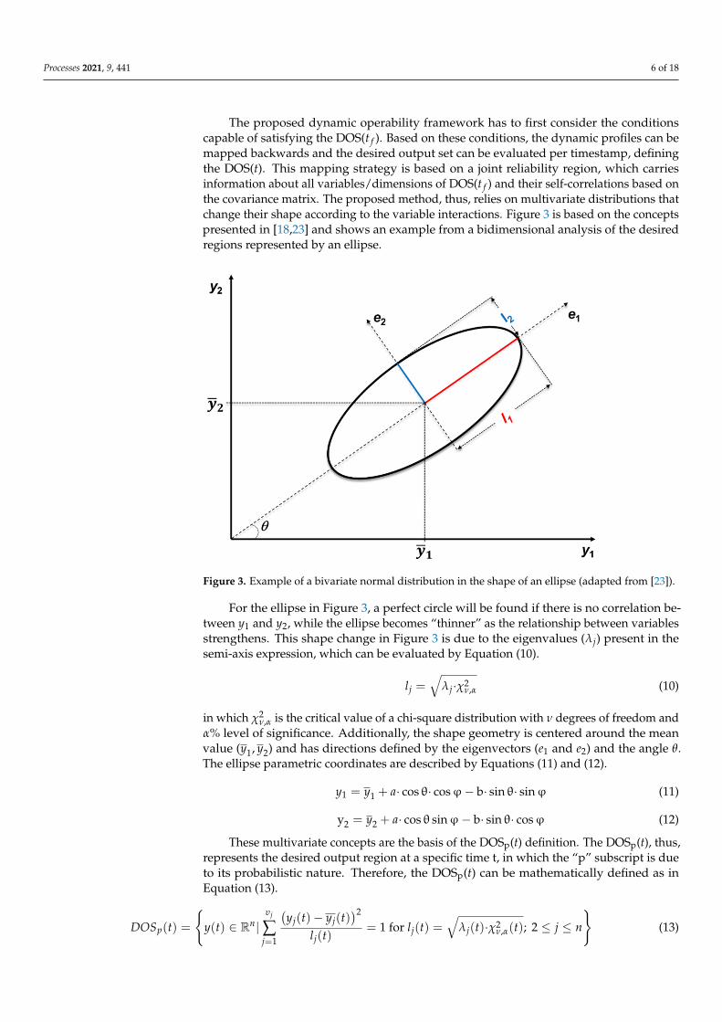
The proposed dynamic operability framework has to first consider the conditionscapable of satisfying the DOS(t f ). Based on these conditions, the dynamic profiles can bemapped backwards and the desired output set can be evaluated per timestamp, definingthe DOS(t). This mapping strategy is based on a joint reliability region, which carriesinformation about all variables/dimensions of DOS(t f ) and their self-correlations based onthe covariance matrix. The proposed method, thus, relies on multivariate distributions thatchange their shape according to the variable interactions. Figure 3 is based on the conceptspresented in [18,23] and shows an example from a bidimensional analysis of the desiredregions represented by an ellipse.

Processes 2021, 9, x FOR PEER REVIEW 6 of 20

lies in the final process specification. Thus, the DOS(𝑡 ) can be defined, where 𝑡 denotes the final time for the same definition as in Equation (5).

The proposed dynamic operability framework has to first consider the conditions capable of satisfying the DOS(𝑡 ). Based on these conditions, the dynamic profiles can be mapped backwards and the desired output set can be evaluated per timestamp, defining the DOS(t). This mapping strategy is based on a joint reliability region, which carries information about all variables/dimensions of DOS(𝑡 ) and their self-correlations based on the covariance matrix. The proposed method, thus, relies on multivariate distributions that change their shape according to the variable interactions. Figure 3 is based on the concepts presented in [18,23] and shows an example from a bidimensional analysis of the desired regions represented by an ellipse.

Figure 3. Example of a bivariate normal distribution in the shape of an ellipse (adapted from [23]).

For the ellipse in Figure 3, a perfect circle will be found if there is no correlation between 𝑦 and 𝑦 , while the ellipse becomes “thinner” as the relationship between variables strengthens. This shape change in Figure 3 is due to the eigenvalues (𝜆 ) present in the semi-axis expression, which can be evaluated by Equation (10). 𝑙 = 𝜆 ∙ 𝜒 , (10)

in which 𝜒 , is the critical value of a chi-square distribution with 𝜈 degrees of freedom and 𝛼% level of significance. Additionally, the shape geometry is centered around the mean value (𝑦 ,𝑦 ) and has directions defined by the eigenvectors (𝑒 and 𝑒 ) and the angle 𝜃. The ellipse parametric coordinates are described by Equations (11) and (12). 𝑦 = 𝑦 𝑎 ∙ cosθ ∙ cosφ − b ∙ sinθ ∙ sinφ (11)y = 𝑦 𝑎 ∙ cosθ sinφ − b ∙ sin θ ∙ cosφ (12)

These multivariate concepts are the basis of the DOSp(t) definition. The DOSp(t), thus, represents the desired output region at a specific time t, in which the “p” subscript is due to its probabilistic nature. Therefore, the DOSp(t) can be mathematically defined as in Equation (13).

Figure 3. Example of a bivariate normal distribution in the shape of an ellipse (adapted from [23]).

For the ellipse in Figure 3, a perfect circle will be found if there is no correlation be-tween y1 and y2, while the ellipse becomes “thinner” as the relationship between variablesstrengthens. This shape change in Figure 3 is due to the eigenvalues (λj) present in thesemi-axis expression, which can be evaluated by Equation (10).

lj =√

λj·χ2ν,α (10)

in which χ2ν,α is the critical value of a chi-square distribution with ν degrees of freedom and

α% level of significance. Additionally, the shape geometry is centered around the meanvalue (y1, y2) and has directions defined by the eigenvectors (e1 and e2) and the angle θ.The ellipse parametric coordinates are described by Equations (11) and (12).

y1 = y1 + a· cos θ· cosϕ− b· sin θ· sinϕ (11)

y2 = y2 + a· cos θ sinϕ− b· sin θ· cosϕ (12)

These multivariate concepts are the basis of the DOSp(t) definition. The DOSp(t), thus,represents the desired output region at a specific time t, in which the “p” subscript is dueto its probabilistic nature. Therefore, the DOSp(t) can be mathematically defined as inEquation (13).

DOSp(t) =

{y(t) ∈ Rn|

υj

∑j=1

(yj(t)− yj(t)

)2

lj(t)= 1 for lj(t) =

√λj(t)·χ2

ν,α(t); 2 ≤ j ≤ n

}(13)

Processes 2021, 9, 441 7 of 18

where n is the DOS dimension; thus, when n = 2, Equation (13) corresponds to an ellipse,n = 3 is an ellipsoid, and so on.

Finally, the dynamic operability index (OI(t)) is evaluated at each timestamp accordingto Equation (14). The lower the OI(t), the more attention is needed in the specific analyzedtime period to guarantee the desired process specification. If no process condition cansatisfy the DOS(t f ), the OI(t f ) is null, resulting in batch run conditions that are not able toachieve the desired specifications.

OI(t) =µ(

AOS(t)⋂

DOSp(t))

µ(

DOSp(t)) (14)

4. Case Study Definition and Setup

This section presents a case study that consists of a pilot batch reactor system. Theproposed operability script for this system is described along with the time-series datasetused. Additionally, the developed dynamic model for this system is validated against thepilot bench unit, producing a digital twin for the process. Following the script, automaticmodel runs are performed considering all of the recipes within a digital experimentationstrategy encompassing 900 simulated conditions (with approximately 1000 generatedpoints per simulated condition), which are defined based on the AIS and the EDSp(t).

4.1. Pilot Batch Unit

The addressed system is characterized by an endothermic second-order reactionbetween sodium hydroxide (NaOH) and ethyl acetate (CH3COOCH2CH3), as describedin Equation (15). This reaction is carried out in a 1.2L stirred batch reactor and followsthe kinetic parameters according to [24]. In this reactor system, water flows in a jacketto transfer enough heat for isothermal operation. A pH indicator is used to mark theend of the reaction process. The experimental apparatus is depicted in Figure 4, wherea thermocouple and an electrical conductivity meter are used to acquire the reactor’stemperature and concentration, respectively.

NaOH + CH3COOCH2CH3 CH3COONa + C2H5OH (15)Processes 2021, 9, x FOR PEER REVIEW 8 of 20

Figure 4. Experimental apparatus associated with the batch reactor case study.

The heating fluid flows in a closed circuit, where electrical resistance is manipulated to control the reactor temperature. A peristaltic pump guarantees its setpoint flow, which is seated in a supervisory control and data acquisition (SCADA) system present in the vendor software and used in the pilot unit operation. The system is also able to acquire the data as a time-series database per batch. The reactants have been previously prepared at determined concentrations and volumes per experiment. The conversion is calculated based on the conductivity measurements, and along with temperature, represents the most relevant variables in the study.

The digital experimentation strategy is delimited by a sensitivity analysis involving different ethyl acetate concentrations (0.1, 0.05, and 0.07 mol/dm3) and temperatures (30, 35, and 40 °C), with a fixed sodium hydroxide concentration of 0.1 mol/dm3. The experimental pilot plant was used to develop and validate a process digital twin, enabling automated and extensive digital manipulation of the system with minimal financial cost and safety risks.

4.2. Dynamic Operability Sets Applied to the Batch Case Study The categorization of the process variables employed is detailed in Table 1, and was

used to define the available input set (AIS), as well as the probabilistic expected disturbance set (EDSp(t)). This categorization is essential when studying the AIS and EDS.

Table 1. Categorization of variables in the AIS and EDS.

Category Variable Description

Static

𝑢 Ethyl acetate initial molar concentration (𝐶 , ) 𝑢 Sodium hydroxide initial molar concentration (𝐶 , ) 𝑢 Initial reactor temperature (𝑇 ) 𝑑 Sodium hydroxide initial volume (𝑉 , ) 𝑑 Ethyl acetate initial volume (𝑉 , )

Dynamic 𝑢 Inlet mass flow of the heating fluid (𝑚 , ) 𝑑 Inlet temperature of the heating fluid (𝑇 , )

The considered AIS has four dimensions, as given in Equation (16), with three static variables, i.e., ones that can only be defined at the beginning of the batch. In particular,

Figure 4. Experimental apparatus associated with the batch reactor case study.

Processes 2021, 9, 441 8 of 18

The heating fluid flows in a closed circuit, where electrical resistance is manipulatedto control the reactor temperature. A peristaltic pump guarantees its setpoint flow, whichis seated in a supervisory control and data acquisition (SCADA) system present in thevendor software and used in the pilot unit operation. The system is also able to acquirethe data as a time-series database per batch. The reactants have been previously preparedat determined concentrations and volumes per experiment. The conversion is calculatedbased on the conductivity measurements, and along with temperature, represents the mostrelevant variables in the study.

The digital experimentation strategy is delimited by a sensitivity analysis involvingdifferent ethyl acetate concentrations (0.1, 0.05, and 0.07 mol/dm3) and temperatures(30, 35, and 40 ◦C), with a fixed sodium hydroxide concentration of 0.1 mol/dm3. Theexperimental pilot plant was used to develop and validate a process digital twin, enablingautomated and extensive digital manipulation of the system with minimal financial costand safety risks.

4.2. Dynamic Operability Sets Applied to the Batch Case Study

The categorization of the process variables employed is detailed in Table 1, and wasused to define the available input set (AIS), as well as the probabilistic expected disturbanceset (EDSp(t)). This categorization is essential when studying the AIS and EDS.

Table 1. Categorization of variables in the AIS and EDS.

Category Variable Description

Static

u1 Ethyl acetate initial molar concentration (CEtAc,0)u2 Sodium hydroxide initial molar concentration (CNaOH,0)u3 Initial reactor temperature (T0)d1 Sodium hydroxide initial volume (VNaOH,0)d2 Ethyl acetate initial volume (VEtAc,0)

Dynamic u4 Inlet mass flow of the heating fluid (.

mw,in)d3 Inlet temperature of the heating fluid (Tw,in)

The considered AIS has four dimensions, as given in Equation (16), with three staticvariables, i.e., ones that can only be defined at the beginning of the batch. In particular, thetwo reactant solutions were previously prepared at specified concentrations. Additionally,the initial reactor temperature depends on the environmental conditions and the heatingsystem capacity.

AIS =

u ∈ R4

∣∣0.05 ≤ u1 ≤ 0.10 mol/dm3;0.05 ≤ u2 ≤ 0.10 mol/dm3;

30 ≤ u3 ≤ 45 ◦C0 ≤ u4 ≤ 10 kg/h

(16)

Equation (17) describes the EDSp. Unlike d3, the two static disturbances (d1 and d2)only need an intensity to be defined in the beginning of the batch, with no duration. Aramp behavior is assumed for the dynamic disturbance to add complexity and simulatethe real case, in which the disturbance first changes from its nominal value and varies to amaximum, where it remains for a certain period until a control system brings it back to itsnominal value. The specifically considered disturbance values are detailed in Table A1 inthe Appendix A.

EDSp(t) =

d(t) ∈ R3

∣∣−100 ≤ d1 ≤ 100 mL with σ1 = 33.33 mL;−100 ≤ d2 ≤ 100 mL with σ2 = 33.33 mL;

−5 ≤ d3 ≤ 5 ◦C with σ3 = 1.67 ◦C

(17)

Processes 2021, 9, 441 9 of 18

The DOS(t f ) is defined by Equation (18), where y1 and y2 correspond to reactorconversion of sodium hydroxide and temperature, respectively. This definition is similar toEquation (5), but related to the batch end time. The batches that satisfy the DOS(t f )—alsoknown as the deterministic desired output set in this work—will serve as basis to calculatethe intermediate DOSp(t)s, i.e., the probabilistic DOS’s.

DOS(

t f

)={

y ∈ R2∣∣∣0.95 ≤ y1 ≤ 1.00 and 40.0 ≤ y2 ≤ 45.0 ◦C

}(18)

4.3. Automated Digital Experimentation

Due to the large number of experiments to be performed, an automated digitalexperimentation strategy is proposed using the Aspen software capability to communicatewith Excel and Visual Basic for Applications (VBA) via Aspen Simulation Workbook(ASW). The batch recipes are defined by a multivariable experimental design formed bycombinations of AIS and EDSp(t), with variables and conditions tabulated in a database.The strategy logics and queue organization are described in the experimentation planning(EP) module in Figure 5, in which a VBA code is written to assemble the recipe specificationsand pass them to the process digital twin (DT) via ASW (Figure 5—step I).

Processes 2021, 9, x FOR PEER REVIEW 10 of 20

Figure 5. Automated digital experimentation flowchart.

The MATLAB code (described in the next section) and VBA dynamic arrays organize the data in a tridimensional way according to Figure 6, where k response variables along time 𝑡 to 𝑡 have the information for the n batches. In such a way, all developed scripts can be expanded to more extensive cases as necessary.

Figure 6. Grid organization for data responses organized by experiment and time.

5. Dynamic Operability Algorithm The dynamic operability analysis is implemented in MATLAB, according to the

diagram described in Figure 7. Essentially, the time-series database is loaded first, the variables are identified, and after a few inputs to the algorithm have been defined, the methodology evaluation is started. These inputs correspond to:

Experimental Design

Variables and conditions specified in AIS and EDSp

i = 0

Restart ABM

i = i + 1

i > if

End

t = 0

t = t + Δt

t > tf

Batch Reactor Model f(t)

Data Reconciliation

Experiment Results

AOS(t)

Experiment i conditions

Databasey (t)

via ASW

via ASW

via ASW

No

YesYes

No

I

III

II

Figure 5. Automated digital experimentation flowchart.

The DT corresponds to an Aspen (ABM) model that provides the results at differenttimestamps because the AspenTech internal numerical method adjusts the time stepsper batch to provide better convergence; hence, the data need to be reconciled beforebeing archived in the final dataset. For this study, around 100 points for 10 variables arestored per one-hour batch. The outputs are sent to the database manager (DM) via ASW(Figure 5—step II). The DM is another VBA script responsible for writing the simulationoutputs that converge in a time-series database. Not necessarily all runs will converge,since the EDSp(t) is pseudo-randomly generated; thus, a condition with no physicalsolution could be found, which would be reported with a trial status. Once the batchreaches the end, a signal is sent to EP via ASW (Figure 5—step III), and then the ABMis reset to start the next simulation. This loop detailed in Figure 5 is repeated until thelast experiment is performed. The complete automated digital experimentation processproduces approximately 900,000 data points.

Processes 2021, 9, 441 10 of 18

The MATLAB code (described in the next section) and VBA dynamic arrays organizethe data in a tridimensional way according to Figure 6, where k response variables alongtime t1 to t f have the information for the n batches. In such a way, all developed scriptscan be expanded to more extensive cases as necessary.

Processes 2021, 9, x FOR PEER REVIEW 10 of 20

Figure 5. Automated digital experimentation flowchart.

The MATLAB code (described in the next section) and VBA dynamic arrays organize the data in a tridimensional way according to Figure 6, where k response variables along time 𝑡 to 𝑡 have the information for the n batches. In such a way, all developed scripts can be expanded to more extensive cases as necessary.

Figure 6. Grid organization for data responses organized by experiment and time.

5. Dynamic Operability Algorithm The dynamic operability analysis is implemented in MATLAB, according to the

diagram described in Figure 7. Essentially, the time-series database is loaded first, the variables are identified, and after a few inputs to the algorithm have been defined, the methodology evaluation is started. These inputs correspond to:

Experimental Design

Variables and conditions specified in AIS and EDSp

i = 0

Restart ABM

i = i + 1

i > if

End

t = 0

t = t + Δt

t > tf

Batch Reactor Model f(t)

Data Reconciliation

Experiment Results

AOS(t)

Experiment i conditions

Databasey (t)

via ASW

via ASW

via ASW

No

YesYes

No

I

III

II

Figure 6. Grid organization for data responses organized by experiment and time.

5. Dynamic Operability Algorithm

The dynamic operability analysis is implemented in MATLAB, according to the dia-gram described in Figure 7. Essentially, the time-series database is loaded first, the variablesare identified, and after a few inputs to the algorithm have been defined, the methodologyevaluation is started. These inputs correspond to:

• Output variables for AOS and DOS;• DOS at the end of the batch (DOS(t f ));• Tolerance allowed (α%) for the joint reliability regions of DOSp(t);• Number of periods used during the process to run the analysis.

Once the dataset is loaded and inputs are defined (Figure 7—step I), all the resultsimpacted by the first disturbance considered are combined (Figure 7—step II) at thebeginning of the process (t0). Then, the AOS(d, t0) is determined (Figure 7—step III) bya MATLAB built-in code called boundary. The Multi-Parametric Toolbox (MPT) was alsotested for this calculation, but the boundary function demonstrated improved behavior inboth convex and non-convex regions. Then, the AOS(t0) is evaluated (Figure 7—step IV)using Equation (9). This procedure is repeated for all predefined periods until the finaltime (t f ). Subsequently, the DOS(t f ) specifications described in Equation (18) are examined(Figure 7—step V). If no output satisfies these limits, the final requirements cannot beachieved by the process under the AIS conditions and considering the disturbances in theEDSp(t). Otherwise, the batches that fulfill the desired set are tracked (Figure 7—step VI)and the DOSp(t f ) is calculated (Figure 7—step VII) via the implementation of Equation (13).Finally, the areas of each AOS(t) and DOSp(t) are determined and the OI(t) is evaluated(Figure 7—step VIII). The last steps (Figure 7—VII and VIII) are repeated backward untilthe first timestamp is achieved.

Processes 2021, 9, 441 11 of 18

Processes 2021, 9, x FOR PEER REVIEW 11 of 20

• Output variables for AOS and DOS; • DOS at the end of the batch (DOS(𝑡 )); • Tolerance allowed (α%) for the joint reliability regions of DOSp(t); • Number of periods used during the process to run the analysis.

Figure 7. Work flow for dynamic operability algorithm.

Once the dataset is loaded and inputs are defined (Figure 7—step I), all the results impacted by the first disturbance considered are combined (Figure 7—step II) at the beginning of the process (𝑡 ). Then, the AOS(𝑑, 𝑡 ) is determined (Figure 7—step III) by a MATLAB built-in code called boundary. The Multi-Parametric Toolbox (MPT) was also tested for this calculation, but the boundary function demonstrated improved behavior in both convex and non-convex regions. Then, the AOS(𝑡 ) is evaluated (Figure 7—step IV) using Equation (9). This procedure is repeated for all predefined periods until the final time ( 𝑡 ). Subsequently, the DOS( 𝑡 ) specifications described in Equation (18) are examined (Figure 7—step V). If no output satisfies these limits, the final requirements cannot be achieved by the process under the AIS conditions and considering the disturbances in the EDSp(t). Otherwise, the batches that fulfill the desired set are tracked (Figure 7—step VI) and the DOSp( 𝑡 ) is calculated (Figure 7—step VII) via the implementation of Equation (13). Finally, the areas of each AOS(t) and DOSp(t) are determined and the OI(t) is evaluated (Figure 7—step VIII). The last steps (Figure 7—VII and VIII) are repeated backward until the first timestamp is achieved.

Identify the variables

Select output

variables

Define theDOS(tf)

Setα% to DOSp(t)

All results at t

AOS(d,t)

AOS(t)

t = tfDOS(tf) cannot

be achieved

t = t - Δt

t = t0

t = t + Δt

Databasey (t)

End

Define number of periods

Evaluate Δt

End

Yes

NoYesNo

No

Yes

II

III

IV

I

TrackN points

VI

DOSp(t)VII

OI(t)VIII

Any point inside DOS(tf)?

V

Figure 7. Work flow for dynamic operability algorithm.

6. Results

Initially, the validation of the digital twin model with the experimental results fromthe pilot plant is presented. Then, the dynamic operability results are shown for differentsets, namely AOS(d,t), DOS(t f ), and DOSp(t), as well as the OI(t) calculations.

6.1. Batch Model Validation with Experimental Results

The batch reactor temperature and sodium hydroxide molar concentration are usedas variables for the model validation. The experiments are conducted until the acid–baseindicator (crystal violet) marks the end of the reaction, with the same experiment durationapplied as for the simulation.

The comparisons between the pilot unit data and the simulated digital twin outcomesare presented for the experiments in Figures 8 and 9. The sodium hydroxide concentrationand reactor temperature profiles are shown in Figure 8a,b respectively for the fixed initialconcentration of ethyl acetate specified in the legend.

The digital twin result profiles in Figure 8 thus closely represent the experimentalones for the entire batch. Specifically, the higher the initial concentration of ethyl acetate(EtAc), the more sodium hydroxide is converted; hence, the sodium hydroxide molarconcentration is lowest when ethyl acetate starts at 0.10 mol/L. The highest relative error(4.0% approximately) occurs at the temperature profile for the lowest ethyl acetate initialconcentration (0.05 mol/dm3); however, this condition did not substantially affect themolar concentration of sodium hydroxide over time.

Processes 2021, 9, 441 12 of 18

Processes 2021, 9, x FOR PEER REVIEW 12 of 20

6. Results Initially, the validation of the digital twin model with the experimental results from

the pilot plant is presented. Then, the dynamic operability results are shown for different sets, namely AOS(d,t), DOS(𝑡 ), and DOSp(t), as well as the OI(t) calculations.

6.1. Batch Model Validation with Experimental Results The batch reactor temperature and sodium hydroxide molar concentration are used

as variables for the model validation. The experiments are conducted until the acid–base indicator (crystal violet) marks the end of the reaction, with the same experiment duration applied as for the simulation.

The comparisons between the pilot unit data and the simulated digital twin outcomes are presented for the experiments in Figures 8 and 9. The sodium hydroxide concentration and reactor temperature profiles are shown in Figures 8a and 8b respectively for the fixed initial concentration of ethyl acetate specified in the legend.

(a)

(b)

Figure 8. Comparison between experimental and simulated results for different ethyl acetate initial concentrations. (a) Molar concentration of sodium hydroxide. (b) Reactor temperature profile.

(a)

(b)

Figure 9. Comparison between experimental and simulated results for setpoint reactor temperature sensitivity analysis. (a) Molar concentration of sodium hydroxide. (b) Reactor temperature profile.

0 0.1 0.2 0.3 0.4 0.5 0.6Time (h)

0

0.01

0.02

0.03

0.04

0.05Exp. [EtAc]0 = 0.05

Sim. [EtAc]0 = 0.05

Exp. [EtAc]0 = 0.07

Sim. [EtAc]0 = 0.07

Exp. [EtAc]0 = 0.10

Sim. [EtAc]0 = 0.10

0 0.1 0.2 0.3 0.4 0.5 0.6Time (h)

20

22

24

26

28

30

32

34

36

38

40

Exp. [EtAc]0 = 0.05

Sim. [EtAc]0 = 0.05

Exp. [EtAc]0 = 0.07

Sim. [EtAc]0 = 0.07

Exp. [EtAc]0 = 0.10

Sim. [EtAc]0 = 0.10

0 0.05 0.1 0.15 0.2 0.25 0.3 0.35Time (h)

0.015

0.02

0.025

0.03

0.035

0.04

0.045

0.05

0.055Exp. T = 30°CSim. T = 30°CExp. T = 35°CSim. T = 35°CExp. T = 40°CSim. T = 40°CExp. T = 45°CSim. T = 45°C

0 0.05 0.1 0.15 0.2 0.25 0.3 0.35Time (h)

26

28

30

32

34

36

38

40

42

44

46Exp. T = 30°CSim. T = 30°CExp. T = 35°CSim. T = 35°CExp. T = 40°CSim. T = 40°CExp. T = 45°CSim. T = 45°C

Figure 8. Comparison between experimental and simulated results for different ethyl acetate initial concentrations. (a) Molarconcentration of sodium hydroxide. (b) Reactor temperature profile.

Processes 2021, 9, x FOR PEER REVIEW 12 of 20

6. Results Initially, the validation of the digital twin model with the experimental results from

the pilot plant is presented. Then, the dynamic operability results are shown for different sets, namely AOS(d,t), DOS(𝑡 ), and DOSp(t), as well as the OI(t) calculations.

6.1. Batch Model Validation with Experimental Results The batch reactor temperature and sodium hydroxide molar concentration are used

as variables for the model validation. The experiments are conducted until the acid–base indicator (crystal violet) marks the end of the reaction, with the same experiment duration applied as for the simulation.

The comparisons between the pilot unit data and the simulated digital twin outcomes are presented for the experiments in Figures 8 and 9. The sodium hydroxide concentration and reactor temperature profiles are shown in Figures 8a and 8b respectively for the fixed initial concentration of ethyl acetate specified in the legend.

(a)

(b)

Figure 8. Comparison between experimental and simulated results for different ethyl acetate initial concentrations. (a) Molar concentration of sodium hydroxide. (b) Reactor temperature profile.

(a)

(b)

Figure 9. Comparison between experimental and simulated results for setpoint reactor temperature sensitivity analysis. (a) Molar concentration of sodium hydroxide. (b) Reactor temperature profile.

0 0.1 0.2 0.3 0.4 0.5 0.6Time (h)

0

0.01

0.02

0.03

0.04

0.05Exp. [EtAc]0 = 0.05

Sim. [EtAc]0 = 0.05

Exp. [EtAc]0 = 0.07

Sim. [EtAc]0 = 0.07

Exp. [EtAc]0 = 0.10

Sim. [EtAc]0 = 0.10

0 0.1 0.2 0.3 0.4 0.5 0.6Time (h)

20

22

24

26

28

30

32

34

36

38

40

Exp. [EtAc]0 = 0.05

Sim. [EtAc]0 = 0.05

Exp. [EtAc]0 = 0.07

Sim. [EtAc]0 = 0.07

Exp. [EtAc]0 = 0.10

Sim. [EtAc]0 = 0.10

0 0.05 0.1 0.15 0.2 0.25 0.3 0.35Time (h)

0.015

0.02

0.025

0.03

0.035

0.04

0.045

0.05

0.055Exp. T = 30°CSim. T = 30°CExp. T = 35°CSim. T = 35°CExp. T = 40°CSim. T = 40°CExp. T = 45°CSim. T = 45°C

0 0.05 0.1 0.15 0.2 0.25 0.3 0.35Time (h)

26

28

30

32

34

36

38

40

42

44

46Exp. T = 30°CSim. T = 30°CExp. T = 35°CSim. T = 35°CExp. T = 40°CSim. T = 40°CExp. T = 45°CSim. T = 45°C

Figure 9. Comparison between experimental and simulated results for setpoint reactor temperature sensitivity analysis. (a)Molar concentration of sodium hydroxide. (b) Reactor temperature profile.

Figures 8 and 9 indicate that the model matches the behavior shown by the experimen-tal results of the pilot unit for all the sensitivity analyses performed for both concentrationand temperature profiles. The highest relative error obtained was around 15% when themolar concentration was below 0.02 and the temperature was at 30 ◦C (see Figure 9), whichis likely related to sensor precision. Thus, as the digital twin (DT) parameters are welladjusted to represent the entire batch system, this DT is used in the proposed dynamicand statistical operability approach. This ABM model is then simulated multiple timesconsidering the cases determined by the design experimentation (see summary in Table A1).In this work, nearly a million data points were generated by the DT, with the correspondingdata stored in a process database.

6.2. Dynamic and Statistical Operability Results

As at t = 0 h, there is no change in the system; the first AOS(d,t) is analyzed att = 0.1 h, as depicted in Figure 10. In this figure, all of the outputs from the simulationsat this timestamp are represented by the markers, while the non-disturbance case, i.e.,AOS (d = 0, t = 0.1 h), is represented by the solid black line. The results from the non-

Processes 2021, 9, 441 13 of 18

disturbance case are plotted along with the ones obtained by the #1 disturbance casefrom Table A1—generating the AOS (d = 9.7, t = 0.1 h)—in Figure 10a.

Processes 2021, 9, x FOR PEER REVIEW 13 of 20

The digital twin result profiles in Figure 8 thus closely represent the experimental ones for the entire batch. Specifically, the higher the initial concentration of ethyl acetate (EtAc), the more sodium hydroxide is converted; hence, the sodium hydroxide molar concentration is lowest when ethyl acetate starts at 0.10 mol/L. The highest relative error (4.0% approximately) occurs at the temperature profile for the lowest ethyl acetate initial concentration (0.05 mol/dm3); however, this condition did not substantially affect the molar concentration of sodium hydroxide over time.

Figures 8 and 9 indicate that the model matches the behavior shown by the experimental results of the pilot unit for all the sensitivity analyses performed for both concentration and temperature profiles. The highest relative error obtained was around 15% when the molar concentration was below 0.02 and the temperature was at 30 °C (see Figure 9), which is likely related to sensor precision. Thus, as the digital twin (DT) parameters are well adjusted to represent the entire batch system, this DT is used in the proposed dynamic and statistical operability approach. This ABM model is then simulated multiple times considering the cases determined by the design experimentation (see summary in Table A1). In this work, nearly a million data points were generated by the DT, with the corresponding data stored in a process database.

6.2. Dynamic and Statistical Operability Results As at t = 0 h, there is no change in the system; the first AOS(d,t) is analyzed at t = 0.1

h, as depicted in Figure 10. In this figure, all of the outputs from the simulations at this timestamp are represented by the markers, while the non-disturbance case, i.e., AOS (d = 0, t = 0.1 h), is represented by the solid black line. The results from the non-disturbance case are plotted along with the ones obtained by the #1 disturbance case from Table A1—generating the AOS (d = 9.7, t = 0.1 h)—in Figure 10a.

(a)

(b)

Figure 10. Points and boundary contours of the achievable output sets at t = 0.1 h. (a) Region representing the initial condition (no disturbance) in black and disturbance #1 (Table A1) in blue. (b) All AOS(d,t = 0.1 h)s determined at 0.1 h and AOS(t = 0.1 h).

Then, the outputs, AOS(d, t = 0.1 h), considering all the disturbance instances (in Table A1) are outlined by the dashed lines (light blue) in Figure 10b. Finally, the AOS(t = 0.1 h) is delimited by the solid line (dark blue) in Figure 10b, where the AOS(t = 0.1 h) is the intersection of all AOS(d,t = 0.1 h)s at 0.1 h and is the one used for operability index (OI) calculation purposes. For this figure, each region was outlined using the MATLAB boundary function, while mathematical operations such as intersections were determined using another built-in MATLAB function called “polybool”.

The procedure above is used to determine the AOS(d,t)s presented in Figure 11a with the output points and AOS(t)s in Figure 11b, at all ten timestamps considered during the

0.5 0.55 0.6 0.65 0.7 0.75 0.8 0.85 0.9 0.95 1Conversion (-)

25

30

35

40

45

50

55

AOS(d=0,t=0.1h)

AOS(d=9.7mL,t=0.1h)

0.5 0.55 0.6 0.65 0.7 0.75 0.8 0.85 0.9 0.95 1Conversion (-)

25

30

35

40

45

50

55

AOS(d,t=0.1h)

AOS(t=0.1h)

Figure 10. Points and boundary contours of the achievable output sets at t = 0.1 h. (a) Region representing the initialcondition (no disturbance) in black and disturbance #1 (Table A1) in blue. (b) All AOS(d,t = 0.1 h)s determined at 0.1 h andAOS(t = 0.1 h).

Then, the outputs, AOS(d, t = 0.1 h), considering all the disturbance instances (in Table A1)are outlined by the dashed lines (light blue) in Figure 10b. Finally, the AOS(t = 0.1 h) is delim-ited by the solid line (dark blue) in Figure 10b, where the AOS(t = 0.1 h) is the intersectionof all AOS(d,t = 0.1 h)s at 0.1 h and is the one used for operability index (OI) calculationpurposes. For this figure, each region was outlined using the MATLAB boundary function,while mathematical operations such as intersections were determined using another built-inMATLAB function called “polybool”.

The procedure above is used to determine the AOS(d,t)s presented in Figure 11a withthe output points and AOS(t)s in Figure 11b, at all ten timestamps considered during thebatch operation. The developed script can consider as many intervals as are available in thedata; however, for visualization purposes, the analysis here is delimited to 10 time instants.

Processes 2021, 9, x FOR PEER REVIEW 14 of 20

batch operation. The developed script can consider as many intervals as are available in the data; however, for visualization purposes, the analysis here is delimited to 10 time instants.

(a)

(b)

Figure 11. Achievable output sets drawn along the batch. (a) Output points, AOS(d,t)s, and AOS(t)s determined at all timestamps considered. (b) AOS(t)s separated for visualization purposes.

The plot of the deterministic desired output set (DOS(𝑡 )) at the end of the batch analyzes whether the designed process can achieve the specifications even with the expected disturbances. By deterministic, it is referred here to the set described by Equation (18), outlined by lower and upper limits and considering no statistical interaction among variables. The output points that satisfy the deterministic DOS(𝑡 ) are indexed and used to build the primary joint reliability region at the final timestamp, i.e., DOSp(𝑡 ), as shown in Figure 12.

Figure 12. Construction of the DOSp(t = 1h) based on the DOS(𝑡 ) defined by specifications.

The DOSp(𝑡 ) is, thus, the tolerance region considered for control purposes, with its center pulled by the region with the highest concentration of data, as shown by the ellipse

10.9

0.820

Conversion (-)

1 0.7

30

0.8

Time (h)

0.6 0.6

40

0.40.2

50

0.50

60

AOS(d=0,t)AOS(d,t)AOS(t)

10.9

0.820

Conversion (-)

1 0.7

30

0.8

Time (h)

0.6 0.6

40

0.40.2

50

0.50

60

Figure 11. Achievable output sets drawn along the batch. (a) Output points, AOS(d,t)s, and AOS(t)s determined at alltimestamps considered. (b) AOS(t)s separated for visualization purposes.

Processes 2021, 9, 441 14 of 18

The plot of the deterministic desired output set (DOS(t f )) at the end of the batch ana-lyzes whether the designed process can achieve the specifications even with the expecteddisturbances. By deterministic, it is referred here to the set described by Equation (18), out-lined by lower and upper limits and considering no statistical interaction among variables.The output points that satisfy the deterministic DOS(t f ) are indexed and used to build theprimary joint reliability region at the final timestamp, i.e., DOSp(t f ), as shown in Figure 12.

Processes 2021, 9, x FOR PEER REVIEW 14 of 20

batch operation. The developed script can consider as many intervals as are available in the data; however, for visualization purposes, the analysis here is delimited to 10 time instants.

(a)

(b)

Figure 11. Achievable output sets drawn along the batch. (a) Output points, AOS(d,t)s, and AOS(t)s determined at all timestamps considered. (b) AOS(t)s separated for visualization purposes.

The plot of the deterministic desired output set (DOS(𝑡 )) at the end of the batch analyzes whether the designed process can achieve the specifications even with the expected disturbances. By deterministic, it is referred here to the set described by Equation (18), outlined by lower and upper limits and considering no statistical interaction among variables. The output points that satisfy the deterministic DOS(𝑡 ) are indexed and used to build the primary joint reliability region at the final timestamp, i.e., DOSp(𝑡 ), as shown in Figure 12.

Figure 12. Construction of the DOSp(t = 1h) based on the DOS(𝑡 ) defined by specifications.

The DOSp(𝑡 ) is, thus, the tolerance region considered for control purposes, with its center pulled by the region with the highest concentration of data, as shown by the ellipse

10.9

0.820

Conversion (-)

1 0.7

30

0.8

Time (h)

0.6 0.6

40

0.40.2

50

0.50

60

AOS(d=0,t)AOS(d,t)AOS(t)

10.9

0.820

Conversion (-)

1 0.7

30

0.8

Time (h)

0.6 0.6

40

0.40.2

50

0.50

60

Figure 12. Construction of the DOSp(t = 1h) based on the DOS(t f ) defined by specifications.

The DOSp(t f ) is, thus, the tolerance region considered for control purposes, with itscenter pulled by the region with the highest concentration of data, as shown by the ellipsein Figure 12. Additionally, the DOSp(t f ) is outlined by considering the tolerance at 60%.The data in Figure 12 are highly concentrated (with many points overlapping each other)at 98–100% conversion and 58–65 ◦C, as well as at 35–45 ◦C and 95–100% conversion,which is the set used to build the DOSp(t f ). Thus, if the desired output set is centered in arange different from these conditions (such as around 47–56 ◦C and 95–100%), the desiredspecifications might not be achieved after a 1 h batch with the AIS and EDSp(t) describedin this work.

With all outputs indexed by timestamp, the other DOSp(t)s can be calculated from thisfinal point, with the indexed data shown in Figure 13.

In the magnified portion in Figure 13, the shape of the joint reliability region is stillcloser to an ellipse at the end of the batch, which indicates a strong correlation betweentemperature and conversion. The funnel-like behavior shown in the figure indicates moredesirable possibilities with a higher probability of occurrence at the beginning of theprocess, followed by the reduction of such possibilities at each time step. This response isdue to the fact that the batch is a time-dependent process that relies on cumulative state-changing behavior along the operation (t). Such a process, thus, becomes more difficult tooperate as it evolves, as also reflected in the decreasing OI(t) values in Table 2.

Processes 2021, 9, 441 15 of 18

Processes 2021, 9, x FOR PEER REVIEW 15 of 20

in Figure 12. Additionally, the DOSp(𝑡 ) is outlined by considering the tolerance at 60%. The data in Figure 12 are highly concentrated (with many points overlapping each other) at 98–100% conversion and 58–65 °C, as well as at 35–45 °C and 95–100% conversion, which is the set used to build the DOSp(𝑡 ). Thus, if the desired output set is centered in a range different from these conditions (such as around 47–56 °C and 95–100%), the desired specifications might not be achieved after a 1 h batch with the AIS and EDSp(t) described in this work.

With all outputs indexed by timestamp, the other DOSp(t)s can be calculated from this final point, with the indexed data shown in Figure 13.

Figure 13. The calculated sequence of DOSp(t)s resulting in funnel-like behavior. This sequence can be used to define regions for batch monitoring and control purposes.

In the magnified portion in Figure 13, the shape of the joint reliability region is still closer to an ellipse at the end of the batch, which indicates a strong correlation between temperature and conversion. The funnel-like behavior shown in the figure indicates more desirable possibilities with a higher probability of occurrence at the beginning of the process, followed by the reduction of such possibilities at each time step. This response is due to the fact that the batch is a time-dependent process that relies on cumulative state-changing behavior along the operation (t). Such a process, thus, becomes more difficult to operate as it evolves, as also reflected in the decreasing OI(t) values in Table 2.

Figure 13. The calculated sequence of DOSp(t)s resulting in funnel-like behavior. This sequence can be used to defineregions for batch monitoring and control purposes.

Table 2. Operability index calculated along batch timestamps.

t (h) µ{AOS(t)} µ{DOSp(t)} OI(t)

0.00 0 0 -0.10 4.6075 0.5359 99.93%0.20 3.3821 0.3740 84.05%0.30 2.2572 0.2898 68.23%0.40 1.5442 0.2373 54.86%0.50 1.1098 0.2006 45.09%0.60 0.8248 0.1731 37.22%0.70 0.6333 0.1522 31.02%0.80 0.6308 0.1359 38.23%0.90 0.6307 0.1222 45.13%1.00 0.6307 0.1119 51.82%

Similarly to the classical operability analysis, the intersections between the AOS(t)sand DOSp(t)s can be evaluated at each timestamp over the batch campaign to provide agraphical idea (as shown in Figure 14) of how much the desired output set is achievableand where to operate the process in order to guarantee the final specifications would bereachable. In particular, the black marker in Figure 14 exemplifies an operation sample of abatch in which the specifications were achieved, even considering the random disturbances.Thus, this process can be characterized as fully dynamically operable in terms of reactorconversion and temperature specifications.

Processes 2021, 9, 441 16 of 18Processes 2021, 9, x FOR PEER REVIEW 17 of 20

Figure 14. Dynamic operability analysis: AOS(t)s, DOSp(t)s, and their intersections over the batch operation. The shaded areas along the campaign represent how much the desired set is achievable.

In case of deviation from the dashed area in Figure 14, the series of regions would serve as a path for the operation to drive the process back to the proper DOSp(t). In order to drive the process back to the desired region in this case, a control system (such as classical feedback or advanced model predictive control) would be required.

7. Conclusions The dynamic operability approach introduced here was applied to a strictly time-

dependent process. The developed method consists of an extension of the classical operability concepts to a scenario where process dynamics and disturbance statistics are considered. The statistical concepts explored included multivariate normal distributions and probabilistic analysis of the expected disturbance set (EDS). A new desired output set (DOSp(t)) was proposed based on the joint reliability region in which the tolerance value α definition is necessary. A procedure to generate a dynamic design space for a batch process in the form of a sequence of regions was provided and can be used in practice to assist batch process operations, monitoring, and control. Such regions consist of desirable and achievable sets at each time step, considering the constraints and the disturbances being assumed as normally distributed. The product specifications are guaranteed at the end of the process if operated inside the intersection series between the AOS and DOS regions.

Figure 14. Dynamic operability analysis: AOS(t)s, DOSp(t)s, and their intersections over the batchoperation. The shaded areas along the campaign represent how much the desired set is achievable.

In case of deviation from the dashed area in Figure 14, the series of regions wouldserve as a path for the operation to drive the process back to the proper DOSp(t). In order todrive the process back to the desired region in this case, a control system (such as classicalfeedback or advanced model predictive control) would be required.

7. Conclusions

The dynamic operability approach introduced here was applied to a strictly time-dependent process. The developed method consists of an extension of the classical op-erability concepts to a scenario where process dynamics and disturbance statistics areconsidered. The statistical concepts explored included multivariate normal distributionsand probabilistic analysis of the expected disturbance set (EDS). A new desired output set(DOSp(t)) was proposed based on the joint reliability region in which the tolerance value αdefinition is necessary. A procedure to generate a dynamic design space for a batch processin the form of a sequence of regions was provided and can be used in practice to assistbatch process operations, monitoring, and control. Such regions consist of desirable andachievable sets at each time step, considering the constraints and the disturbances beingassumed as normally distributed. The product specifications are guaranteed at the end ofthe process if operated inside the intersection series between the AOS and DOS regions.

The process model developed for the performed batch case study was validatedwith experiments from a pilot plant. This model was defined as the digital twin for thebatch process, and an automated digital experimentation strategy was proposed in anIndustry 4.0 framework. The success of the analysis performed here depends on the datasource reliability and quality generated by the digital twin. The methodology accuracyis improved as more data are available, and from this perspective a plant informationmanagement system (PIMS) can be a powerful tool for operability studies. In future work,the authors plan to integrate the current solution with alarms and message notificationswhenever the dynamic operability methodology detects operational actions necessary forthe process to return to an operable state.

Author Contributions: This paper is a collaborative work among the authors. W.R.d.A. performedall simulations and wrote the manuscript. H.B. and F.V.L. helped with the analysis and supervision

Processes 2021, 9, 441 17 of 18

of the research work and with the paper writing and oversaw all technical aspects. All authors haveread and agreed to the published version of the manuscript.

Funding: This study was financed in part by the Coordenação de Aperfeiçoamento de Pessoal deNível Superior—Brazil (CAPES)—Finance Code 001.

Institutional Review Board Statement: Not applicable.

Informed Consent Statement: Not applicable.

Data Availability Statement: Not applicable.

Acknowledgments: The authors thank the Chemical Engineering Department at the Federal Univer-sity of Campina Grande for the instrumentation and materials used for experiments.

Conflicts of Interest: The authors declare no conflict of interest.

Appendix A

Table A1. Different disturbances in EDSp(t) in the dynamic operability analysis.

N Disturbance % of Beginning Intensity from Nominal Value Time Span (min)

1d1 (mL)

0 9.70 02 0 −12.24 03 0 −16.43 0

4d2 (mL)

0 −73.81 05 0 49.99 06 0 −15.66 0

7

d3 (◦C)

0 1.52 58 0 1.52 159 0 1.52 3010 0 −3.15 511 0 −3.15 1512 0 −3.15 3013 0 4.17 514 0 4.17 1515 0 4.17 3016 25 1.52 517 25 1.52 1518 25 1.52 3019 25 −3.15 520 25 −3.15 1521 25 −3.15 3022 25 4.17 523 25 4.17 1524 25 4.17 3025 50 1.52 526 50 1.52 1527 50 1.52 3028 50 −3.15 529 50 −3.15 1530 50 −3.15 3031 50 4.17 532 50 4.17 1533 50 4.17 3034 75 1.52 535 75 1.52 1536 75 −3.15 537 75 −3.15 1538 75 4.17 539 75 4.17 15

Processes 2021, 9, 441 18 of 18

References1. Vinson, D.R.; Georgakis, C. A new measure of process output controllability. J. Process Control 2000, 10, 185–194. [CrossRef]2. Lima, F.V.; Jia, Z.; Ierapetritou, M.; Georgakis, C. Similarities and Differences between the Concepts of Operability and Flexibility:

The Steady-State Case. AIChE J. 2010, 56, 702–716. [CrossRef]3. Carrasco, J.C.; Lima, F.V. Bilevel and Parallel Programing-Based Operability Approaches for Process Intensification and Modular-

ity. AIChE J. 2018, 64, 3042–3054. [CrossRef]4. Shead, L.R.E.; Anastassakis, C.G.; Rossiter, J.A. Steady-state operability of multi-variable non-square systems: Application

to Model Predictive Control (MPC) of the Shell Heavy Oil Fractionator (SHOF). In Proceedings of the 2007 MediterraneanConference on Control & Automation, Athens, Greece, 27–29 June 2007; pp. 1–6.

5. Lima, F.V.; Georgakis, C.; Smith, J.F.; Schnelle, P.D.; Vinson, D.R. Operability-Based Determination of Feasible Control Constraintsfor Several High-Dimensional Nonsquare Industrial Processes. AIChE J. 2010, 56, 1249–1261. [CrossRef]

6. Carrasco, J.C.; Lima, F.V. An optimization-based operability framework for process design and intensification of modular naturalgas utilization systems. Comput. Chem. Eng. 2017, 105, 246–258. [CrossRef]

7. Bishop, B.A.; Lima, F.V. Modeling, Simulation, and Operability Analysis of a Nonisothermal, Countercurrent, Polymer MembraneReactor. Processes 2020, 8, 78. [CrossRef]

8. Carrasco, J.C.; Lima, F.V. Nonlinear Operability of a Membrane Reactor for Direct Methane Aromatization. In Proceedings of the9th IFAC ADCHEM Symposium, Whistler, BC, Canada, 7–10 June 2015; Volume 48, pp. 728–733.

9. Gazzaneo, V.; Carrasco, J.C.; Vinson, D.R.; Lima, F.V. Process Operability Algorithms: Past, Present, and Future Developments.Ind. Eng. Chem. Res. 2020, 59, 2457–2470. [CrossRef]

10. Subramanian, S.; Georgakis, C. Steady-state operability characteristics of idealized reactors. Chem. Eng. Sci. 2001, 56, 5111–5130.[CrossRef]

11. Lima, F.V.; Georgakis, C. Design of output constraints for model-based non-square controllers using interval operability. J. ProcessControl 2008, 18, 610–620. [CrossRef]

12. Lima, F.V.; Georgakis, C. Input–Output Operability of Control Systems: The Steady-State Case. J. Process Control 2010, 20, 769–776.[CrossRef]

13. Georgakis, C.; Uztürk, D.; Subramanian, S.; Vinson, D.R. On the operability of continuous processes. Control Eng. Pract. 2003, 11,859–869. [CrossRef]

14. Uztürk, D.; Georgakis, C. Inherent Dynamic Operability of Processes: General Definitions and Analysis of SISO Cases. Ind. Eng.Chem. Res. 2002, 41, 421–432. [CrossRef]

15. Gazzaneo, V.; Lima, F.V. Multilayer Operability Framework for Process Design, Intensification, and Modularization of NonlinearEnergy Systems. Ind. Eng. Chem. Res. 2019, 58, 6069–6079. [CrossRef]

16. Lima, F.V.; Georgakis, C. Dynamic Operability for the Calculation of Transient Output Constraints for Non-Square Linear ModelPredictive Controllers. In Proceedings of the 7th IFAC ADCHEM Symposium, Istanbul, Turkey, 12–15 July 2009; Volume 42,pp. 231–236.

17. Chen, Y.; Durango-Cohen, P.L. Development and Field Application of a Multivariate Statistical Process Control Framework forHealth-Monitoring of Transportation Infrastructure. Transp. Res. Part B Methodol. 2015, 81, 78–102. [CrossRef]

18. Kharbach, M.; Cherrah, Y.; Heyden, Y.V.; Bouklouze, A. Multivariate Statistical Process Control in Product Quality ReviewAssessment—A Case Study. Ann. Pharm. Françaises 2017, 75, 446–454. [CrossRef] [PubMed]

19. Almeida, F.A.; Leite, R.R.; Gomes, G.F.; Gomes, J.H.F.; Paiva, A.P. Multivariate Data Quality Assessment Based on Rotated FactorScores and Confidence Ellipsoids. Decis. Support Syst. 2020, 129, 113173. [CrossRef]

20. Soroush, M.; Kravaris, C. Optimal design and operation of batch reactors. 1. Theoretical framework. Ind. Eng. Chem. Res. 1993,32, 866–881. [CrossRef]

21. Soroush, M.; Kravaris, C. Optimal design and operation of batch reactors. 2. A case study. Ind. Eng. Chem. Res. 1993, 32, 882–893.[CrossRef]

22. Herceg, M.; Kvasnica, M.; Jones, C.N.; Morari, M. Multi-Parametric Toolbox 3.0. In Proceedings of the European ControlConference, Zurich, Switzerland, 17–19 July 2013; pp. 502–510.

23. STAT 505: Applied Multivariate Statistical Analysis. Available online: https://onlinecourses.science.psu.edu/stat505/ (accessedon 15 May 2020).

24. Das, K.; Sahoo, P.; Baba, M.S.; Murali, N.; Swaminathan, P. Kinetic studies on saponification of ethyl acetate using an innovativeconductivity-monitoring instrument with a pulsating sensor. Int. J. Chem. Kinet. 2011, 43, 648–656. [CrossRef]