Dynamic Analysis - Harvard John A. Paulson School of ...

Dynamic Analysis

CS252r Fall 2015

Stephen Chong, Harvard University

Reading

•The Concept of Dynamic Analysis by Thomas Ball, FSE 1999

•Efficient Path Profiling by Thomas Ball and James Larus, MICRO 1996

•Adversarial Memory for Destructive Data Races by Cormac Flanagan and Stephen Freund, PLDI 2010

2


Dynamic Analysis

•Analysis of the properties of a running program •Static analysis typically finds properties that hold

of all executions •Dynamic analysis finds properties that hold of one

or more executions •Can't prove a program satisfies a particular property •But can detect violations and provide useful information

•Usefulness derives from precision of information and dependence on inputs

3


Precision of Information

•Dynamic analysis typically instructs program to examine or record some of run-time state

•Instrumentation can be tuned to precisely data needed for a problem

4


Dependence on Program Inputs

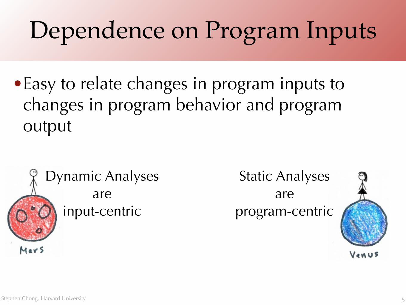
•Easy to relate changes in program inputs to changes in program behavior and program output

5

Dynamic Analyses are

input-centric

Static Analyses are

program-centric


Complementary Techniques

•Completeness •Dynamic analyses can generate "dynamic program invariants", i.e.,

invariants of observed execution; static analyses can check them •Dynamic analyses consider only feasible paths (but may not

consider all paths); static analyses consider all paths (but may include infeasble paths)

•Scope •Dynamic analyses examine one very long program path •Can discover semantic dependencies widely separated in path and in time

• Static analyses typically and at discovering "dependence at a distance"

•Precision

6


Two (plus a bonus) Dynamic Analyses

•Frequency Spectrum Analysis •Efficient path profiling

•Dynamic race detection

7


Frequency Spectrum Analysis

•Understanding frequency of execution of program parts can help programmer: •partition program by levels of abstraction •find related computations •find computations related to specific attributes of input

or output

8


Understanding an Obfuscated C Program

9

#include <stdio.h>main(t,_,a)char *a;{return!0<t?t<3?main(-79,-13,a+main(-87,1-_,main(-86,0,a+1)+a)):1,t<_?main(t+1,_,a):3,main(-94,-27+t,a)&&t==2?_<13?main(2,_+1,"%s %d %d\n"):9:16:t<0?t<-72?main(_,t,"@n'+,#'/*{}w+/w#cdnr/+,{}r/*de}+,/*{*+,/w{%+,/w#q#n+,/#{l+,/n{n+,/+#n+,/#\;#q#n+,/+k#;*+,/'r :'d*'3,}{w+K w'K:'+}e#';dq#'l \q#'+d'K#!/+k#;q#'r}eKK#}w'r}eKK{nl]'/#;#q#n'){)#}w'){){nl]'/+#n';d}rw' i;#\){nl]!/n{n#'; r{#w'r nc{nl]'/#{l,+'K {rw' iK{;[{nl]'/w#q#n'wk nw' \iwk{KK{nl]!/w{%'l##w#' i; :{nl]'/*{q#'ld;r'}{nlwb!/*de}'c \;;{nl'-{}rw]'/+,}##'*}#nc,',#nw]'/+kd'+e}+;#'rdq#w! nr'/ ') }+}{rl#'{n' ')# \}'+}##(!!/"):t<-50?_==*a?putchar(31[a]):main(-65,_,a+1):main((*a=='/')+t,_,a+1):0<t?main(2,2,"%s"):*a=='/'||main(0,main(-61,*a,"!ek;dc i@bK'(q)-[w]*%n+r3#l,{}:\nuwloca-O;m .vpbks,fxntdCeghiry"),a+1);}


What it does...

10

$ gcc -w obfus.c $ ./a.out On the first day of Christmas my true love gave to mea partridge in a pear tree.

On the second day of Christmas my true love gave to metwo turtle dovesand a partridge in a pear tree.

On the third day of Christmas my true love gave to methree french hens, two turtle dovesand a partridge in a pear tree.


Program understanding

•We know what the program does •Our aim is to understand how it does it •Before reverse engineering it, let's have a model in mind:

•Gift t mentioned 13-t times in the poem (e.g. "five gold rings" occurs 13-5=8 times) •So 1+2+...+11+12 = 13*6 = 78 gift mentions (66 mentions of non-partridge gifts) •All verses except first have form

On the <ordinal> day of Christmas my true love gave to me <list of gift phrases, from the ordinal day down to the second day> and a partridge in a pear tree.and first verse is On the first day of Christmas my true love gave to me a partridge in a pear tree.

•Unique strings: • 3 strings for common structure ("On the", "day of Christmas...", "and a partridge ...")

• 12 strings for the ordinals

• 11 strings for the second through twelfth gifts.

•⇒approx. 3+12+11 = 26 unique strings in program, prints approx. 3*12 + 12 + 66 = 114 strings.

11


Model

•12 days of Christmas (also 11, to catch "off-by-one" cases)

•26 unique strings •66 occurrences of non-partridge-in-a-pear-tree

presents •114 strings printed, and •2358 characters printed.

12


Program understanding

•First let's make it readable:

13

It's a single recursive function!


Path Profiling

•Count executions of paths of the function •E.g., path executed 2358 times likely involved in printing characters

14

Stephen Chong, Harvard University 15

PUSH!

Path Profiling Efficient Path Profiling, Ball and Larus, MICRO 1996


Problem: path profiling

•Which paths through a procedure are most common? •e.g., perform aggressive optimization on hot paths, make sure all

paths are tested.

•Naive approach: count edge transitions

•Not enough information to determine paths!16

Efficient Path Profiling

Thomas Ball Bell Laboratories

Lucent Technologies tball @research.bell-labs.com

Abstract

A path profile determines how many times each acyclic path in a routine executes. This type of profiling subsumes the more common basic block and edge profiling, which only approximate path frequencies. Path profiles have many potential uses in program performance tuning, profile-directed compilation, and software test coverage.

This paper describes a new algorithm for path projling. This simple, fast algorithm selects andplacesprojile instrumentation to minimize run-time overhead. Instrumented programs run with overhead comparable to the best previous profiling techniques. On the SPEC95 benchmarks, path projling overhead averaged 31%, as compared to 16% for eficient edge projiling. Path profiling also identifies longer paths than a previous technique, which predicted paths from edge profiles (average of 88, versus 34 instructions). More- over; profiling shows that the SPEC95 train input datasets covered most of the paths executed in the ref datasets.

1 Introduction

Program profiling counts occurrences of an event during a program’s execution. Typically, the measured event is the execution of a local portion of a program, such as a routine or line of code. Recently, fine-grain profiles-of basic blocks and control-flow edges-have become the basis for profile-driven compilation, which uses measured frequencies to guide compilation and optimization.

*This research supported by: Wright Laboratory Avionics Directorate, Air Force Material Command, USAF, under grant #F33615-94-l- 1525 and ARPA order no. B550; NSF NY1 Award CCR-9357779, with support from Hewlett Packard, Sun Microsystems, and PGI; NSF Grant MIP-9225097; and DOE Grant DE-FG02-93ER25176. The U.S. Government is authorized to reproduce and distribute reprints for Governmental purposes notwithstanding any copyright notation thereon. The views and conclusions contained herein are those of the authors and should not be interpreted as necessarily representing the official policies or endorsements, either expressed or implied, of the Wright Laboratory Avionics Directorate or the U. S. Government.

James R. Larus* Dept. of Computer Sciences

University of Wisconsin-Madison [email protected]

Path FTofl Froa

ACDF 90 110 ACDEF 60 40 ABCDF 0 0 ABCDEF 100 100 ABDF 20 0 ABDEF 0 20

Figure 1. Example in which edge profiling does not identify the most frequently executed paths. The table contains two different path profiles. Both path profiles induce the same edge execution frequencies, shown by the edge frequencies in the control-flow graph. In path profile Profl, path ABCDEF is most frequently executed, although the heuristic of following edges with the highest frequency identifies path ACDEF as the most frequent.

One use of profile information is to identify heavily executed paths (or traces) in a program [Fis81, E1185, Cha88, YS94]. Unfortunately, basic block and edge profiles, although inexpensive and widely available, do not always correctly predict frequencies of overlapping paths. Consider, for example, the control-flow graph (CFG) in Figure 1. Each edge in the CFG is labeled with its frequency, which nor- mally results from dynamic profiling, but in the figure is induced by both path profiles in the table. A commonly used heuristic to select a heavily executed path follows the most frequently executed edge out of a basic block [Cha88], which identifies path ACDEF. However, in path profile Profl, this path executed only 60 times, as compared to 90 times for path ACDF and 100 times for path ABCDEF. In profile Prof 2, the disparity is even greater although the edge profile is exactly the same.

This inaccuracy is usually ignored, under the assumption that accurate path profiling must be far more expensive than basic block or edge profiling. Path profiling is the ul- timate form of control-flow profiling, as it uniquely deter-

46 1072-4451/96 $5.00 0 1996 IEEE




Abstract



1 Introduction





Path FTofl Froa





46 1072-4451/96 $5.00 0 1996 IEEE




Abstract



1 Introduction





Path FTofl Froa





46 1072-4451/96 $5.00 0 1996 IEEE



•(For DAGs) •Encode each path as a unique integer and record

path as state •i.e., at end of DAG, value of a register identifies path

through DAG

17

mines both basic block and edge profiles, although the con- verse does not hold, as Figure 1 shows. Also, the number of blocks or edges in a program is finite and linear in the program’s size, but a program with loops offers an unbounded number of potential paths. Considering only acyclic paths bounds this set, but, in the worst case, its size is still expo- nential in the program’s size.

This paper shows that accurate profiling is neither complex nor expensive. It describes a new and efficient technique for path profiling. Our algorithm places instrumentation that accurately determines dynamic execution frequency of control-flow paths in a routine. The instrumentation is not only simple and low-cost, but it is placed in a way that minimizes its overhead. Remarkably, although path profiling collects far more information than block or edge profiling, its overhead can be lower and is usually comparable-on the SPEC95 benchmarks, path profiling’s average overhead is 3 1 %, while efficient edge profiling’s overhead is 16%.

Efficient path profiling opens new possibilities for program optimization and performance tuning. Instead of rely- ing on heuristics, which fully predict only 38% of the executed acyclic paths in the SPEC95 benchmarks, profile- driven compilers can base their decisions on accurate measurements.

Another potential application of path profiling is software test coverage, which quantifies the adequacy of a test data set by profiling a program and reporting unexecuted statements or control-flow. Few, if any, coverage tools measure path coverage. Instead, tools rely on weaker criteria, such as statement or control-flow edge coverage. Edge profiling is less complete than path profiling, as shown in Figure 1, where the two path profiles cover different sets of paths yet induce the same edge profile. Besides an efficient algorithm for path profiling, this paper also presents measurements that show that most routines in a small sample of programs have few (< 3000) potential paths, so that path coverage testing could be feasible for large portions of a program. On the other hand, the measurements also demonstrate the difficulty of developing test data sets, since the programs as a whole executed an average of 2696 paths (249-24414), as compared to the millions of potential paths identified by the path profiling algorithm.

1.1 Algorithm Overview

The essential idea behind the path profiling algorithm is to identify sets of potential paths with states, which are en- coded as integers. Consider for a moment a routine without a loop. Upon entry to the routine, all paths are possible. Taking a conditional branch narrows the set of potential paths and corresponds to a transition to a new state. At the routine’s exit, the final state represents the single path taken

L-h. r=O

B r=2 '

r=4

Ii?3 D r+=l

E F

I Path Encoding

ACDF 0 ACDEF 1 ABCDF 2 ABCDEF 3 ABDF 4 ABDEF 5

ccnmt [x-l++

Figure 2. Path profiling instrumentation. Each path from A to F produces a unique state in register r, which indexes an array of counters in F.

through the routine. This paper presents an efficient algorithm that:

l Numbers final states from 0. . . n - 1, where n is the number of potential paths in a routine. With this compact numbering, a final state can directly index an array of counters.

l Places instrumentation so that transitions need not occur at every conditional branch.

l Assigns states so that transitions can be computed by a simple arithmetic operation, without an explicit state transition table or memory reference.

l Transforms a control-flow graph containing loops or huge numbers of potential paths into an acyclic graph with a limited number of paths.

Figure 2 illustrates the technique. Edges labeled by small squares contain instrumentation, which updates the state in register T. The loop contains six unique paths, and each one computes a different value for T, as shown in the table. At the end of the loop body (block F), register r holds the index to increment an array of counters.

1.2 Extensions

The algorithm in this paper can be easily extended in several ways. First, instead of intraprocedural profiling, it could be applied to a program’s call graph, to record call paths. An interesting complication is indirect calls, which require a dynamic data structure to record calls along edges that are not in the call graph.

Also, instead of just counting the number of times a path executes, the profiling algorithm can easily accumulate a metric for a path. Some processors provide accessible counters for metrics such as the number of processor cycles,


Algorithm overview

•1. Number paths uniquely •2. Use spanning tree to select edges to

instrument (and compute appropriate increment for each instrumented edge)

•3. Select appropriate instrumentation •4. After profiling, given path number, figure out

which path it corresponds to

18


Compact path numbering

•Aim: assign non-negative constant value to each edge such that sum of values along any path from ENTRY to EXIT is unique. Moreover, path sums should be in range 0..(NumPaths - 1) (i.e., minimal encoding)

19


Compact path numbering

20

____ ---_ .-- --__ . --- --” if v is a leaf vertex A

NumPaths(v) = 1; 2 0

) else { 3: I3 0 c vertex v maths W

NumPaths(v) = 0; 6 for each edge e = v->w C 2 4

Val (e) = NumPathsCv); 0 2

NumPaths(v) = NumPathsCv) + NumPathsCw); n LEJ

2 .

Figure 5. Algorithm for assigning values to edges in a DAG.

edges. If T is the set of spanning tree edges, then any graph edge not in T is a chord of the spanning tree.

For example, in the graph of Figure 2, vertex A is the ENTRY vertex and vertex F is the EXIT vertex. The un- adorned graph edges comprise a spanning tree. The edges labeled by squares are chords of the spanning tree.

3.2 Compactly Representing Paths with Sums

The first step in path profiling is to assign a non-negative constant value VaZ(e) to each edge e in a DAG, such that the sum of values along any path from ENTRY to EXIT is unique. Furthermore, the path sums should lie in the range from 0 to the number of paths (minus one), so that the encoding is minimal.

The algorithm in Figure 5 computes such a VaZ relation by visiting vertices of the DAG in reverse topological order. This order ensures that all the successors of a vertex ZJ are visited before ‘u itself. Associated with each vertex v is a value NumPaths(v), which records the number of paths from u to EXIT. The algorithm is simple. At vertex v, the algorithm visits all of v’s outgoing edges v + wi, 1 < i 5 n, and assigns the lath outgoing edge the value:

Val(v + wk) = Cti; NumPaths(wi)

The following theorem proves the algorithm correct:

Theorem 1 Given a DAG, after the algorithm of Figure 5 visits vertex u, NumPaths(v) is the number of paths from u to EXIT and each path from v to EXIT generates a unique value sum in the range 0.. . NumPaths(v) - 1.

Proof. By induction on the height of a vertex in the DAG (i.e., the max number of steps to the sink vertex EXIT).

Base Case: v has height equal to zero (that is, v = EXIT), so NumPaths(v) = 1. The theorem is trivially satisfied.

Figure 6. Control-flow graph from Figure 1, with values computed by the algorithm in Figure 5.

Induction Step: Show that the theorem holds for any vertex v of height H (H > 0). All successors ~1 . . . W, of v must have height less than H (because the graph is a DAG), so the theorem holds for all WJ~. It is trivial to see that the number of paths from v to EXIT is Cy=‘=, NumPaths(wi), which the algorithm computes. By the induction hypothesis, each path from Wk to EXIT generates a unique value sum in the range 0. . . NumPaths(wk) - 1. There- fore, any path from v to EXIT starting with edge v -+ wk will generate a unique value in the range C;“-i’ NumPaths(w;) . . . (CF=, NumPaths(wi)) - 1. Since all NumPaths(wi) values are greater than 0, it follows that no two paths from v to EXIT generate the same value sum. 0

Figure 6 illustrates how the algorithm operates on the example control-flow graph. Note that vertices are labeled in topological ordering, so FEDCBA is a reverse topological order. Any vertex with a single outgoing edge e, such as C and E, always has VaZ(e) = 0.

3.3 Efficiently Computing Sums

Given an edge value assignment, the second step of the algorithm finds a minimal cost set-with respect to a weighting (Section 3)-of edges along which to compute these values, while preserving the two properties of the value assignment.

This step of the algorithm finds a maximal cost spanning tree of the graph (to find a minimal cost set of chord edges), and applies an efficient event counting technique [Ba194] to determine the increment Inc(c) for each chord c in a spanning tree. The event counting algorithm ensures that the sum of Inc values for any path P from ENTRY to EXIT is identical to the sum of Val values for P. Note that some of the Inc values may be negative, as in Figure 4. The edge EXIT -+ ENTRY is required for this step (if this edge is

50







2 .


















50

A 0

B C 2

$3 4 D

1

E F

A 4

B C -2

B 0 D

1

E F

A 5 1

B C -2

33 D -1

E F

b) Cb) (c)

Figure 4. Three possible placements of instrumentation for the control-flow graph from Figure 1.

way branch [BL94, Bal96]. When a branch executes, instrumentation code appends a bit to a trace buffer that records branch outcomes. By recording multiple bits, the approach can be extended to multi-way branches. The contents of the buffer form an index into an array or as a hash value.

It is easy to see that bit tracing uses the minimal number of bits necessary to distinguish paths. For simple control- flow graphs, such as a chain of if-then-else statements, bit tracing, like our approach, produces a compact representations of paths. However, in general, bit tracing may not yield the most compact representations of paths possible. It is easy to construct examples for which the maximal path value under bit tracing is not minimal, no matter the choice of bit labellings. In the worst case, the number of entries in an array of counters may be twice our method.

In addition, bit tracing is likely to have higher run-time overhead than our approach. First, every predicate must be instrumented, whereas our approach allows flexibility in placing instrumentation to reduce overhead. Second, on most machines, the instrumentation to append to a bit string is more complex and slower than a register-to-register addition.

3 Path Profiling of DAGs

As described previously, path profiling tracks a path in a directed acyclic graph (DAG) by updating a register along certain edges of the DAG. This section shows how to compute the necessary updates, efficiently place instrumentation, and derive an executed path from the resulting profile.

The example in Figure 4 shows that many placements of instrumentation yield equivalent results. However, some placements incur less run-time overhead than others. For example, all three graphs in Figure 4 produce the same sum along any acyclic path from A to F. However, in graph (a), the largest number of instrumented edges on any path from A to F is two, while graphs (b) and (c) have up to four and three, respectively.

The path profiling algorithm first labels edges in a DAG

with integer values, such that each path from the entry to the exit of the DAG produces a unique sum of the edge values along that path (the path sum). However, placements from this step may have sub-optimal run-time overhead, as above.

In the next step, another algorithm [Bal94] improves this computation, by finding an equivalent computation that uses a minimal number of additions along DAG edges that are not in the DAG’s spanning tree. In each graph in Figure 4, the uninstrumented edges (those without squares along them) form a spanning tree. Since a DAG may have many spanning trees, the algorithm has the freedom to place instrumentation along edges less likely to be executed.’

After reviewing the basic graph terminology in Sec- tion 3.1, this section describes the four basic steps to path profile a DAG:

1.

2.

3.

4.

3.1

Assign integer values to edges such that no two paths compute the same path sum (Section 3.2). This encoding is minimal.

Use a spanning tree to select edges to instrument and compute the appropriate increment for each instrumented edge (Section 3.3).

Select appropriate instrumentation (Section 3.4).

After collecting the run-time profile, derive the executed paths (Section 3.5).

Terminology

For the remainder of this paper, unless otherwise noted, control-flow graphs (CFGs) have been converted into directed acyclic graphs (DAG) with a unique source vertex ENTRY and sink vertex EXIT. Section 4 shows how to transform an arbitrary CFG into a DAG, which can be path profiled. For technical reasons, the increment computation (Section 3.3) requires a “dummy” edge EXIT + ENTRY (although this creates an unexecutable cycle, the graph can still be treated as a DAG by ignoring this backedge).

An execution of a DAG produces an acyclic, directed path starting at ENTRY and ending at EXIT. The term path refers to an acyclic directed path, unless otherwise noted. Of course, a DAG may execute many times, as it may consist of a loop body or a procedure.

A spanning tree of a graph G is a subgraph that is a tree and contains all vertices of G. Edges in a spanning tree are bidirectional and need not follow the direction of graph

‘This approach requires computing (or obtaining from a profile) a weight for each edge that statically approximates the edge’s execution frequency. A maximum spanning tree of the graph, with respect to that weighting, maximizes the weight (execution frequency) of the uninstm- mented edges. PP uses the same previously published, effective algorithm for statically computing a weighting as QPT [BL94].

49


Efficiently compute sums

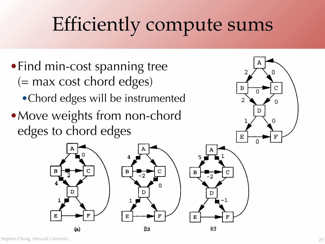
•Find min-cost spanning tree(= max cost chord edges) •Chord edges will be instrumented

•Move weights from non-chord edges to chord edges

21







2 .


















50


Instrumentation

•Needed instrumentation: •Initialize path register (r = 0) at ENTRY

•Increment register on instrumented edges (r += Inc(e))

•Record path's counter at EXIT (count[r]++)

•Can optimize: •Chord edge e can initialize counter (r = Inc(e)) iff first

chord edge on every path from ENTRY to EXIT containing e •Chord edge e may increment path register and memory

counter (count[r+Inc(e)]++) iff last chord edge on every path from ENTRY to EXIT containing e

22


Instrumentation

23

A 0

B C 2

$3 4 D

1

E F

A 4

B C -2

B 0 D

1

E F

A 5 1

B C -2

33 D -1

E F

b) Cb) (c)

Figure 4. Three possible placements of instrumentation for the control-flow graph from Figure 1.

way branch [BL94, Bal96]. When a branch executes, instrumentation code appends a bit to a trace buffer that records branch outcomes. By recording multiple bits, the approach can be extended to multi-way branches. The contents of the buffer form an index into an array or as a hash value.

It is easy to see that bit tracing uses the minimal number of bits necessary to distinguish paths. For simple control- flow graphs, such as a chain of if-then-else statements, bit tracing, like our approach, produces a compact representations of paths. However, in general, bit tracing may not yield the most compact representations of paths possible. It is easy to construct examples for which the maximal path value under bit tracing is not minimal, no matter the choice of bit labellings. In the worst case, the number of entries in an array of counters may be twice our method.

In addition, bit tracing is likely to have higher run-time overhead than our approach. First, every predicate must be instrumented, whereas our approach allows flexibility in placing instrumentation to reduce overhead. Second, on most machines, the instrumentation to append to a bit string is more complex and slower than a register-to-register addition.

3 Path Profiling of DAGs

As described previously, path profiling tracks a path in a directed acyclic graph (DAG) by updating a register along certain edges of the DAG. This section shows how to compute the necessary updates, efficiently place instrumentation, and derive an executed path from the resulting profile.

The example in Figure 4 shows that many placements of instrumentation yield equivalent results. However, some placements incur less run-time overhead than others. For example, all three graphs in Figure 4 produce the same sum along any acyclic path from A to F. However, in graph (a), the largest number of instrumented edges on any path from A to F is two, while graphs (b) and (c) have up to four and three, respectively.

The path profiling algorithm first labels edges in a DAG

with integer values, such that each path from the entry to the exit of the DAG produces a unique sum of the edge values along that path (the path sum). However, placements from this step may have sub-optimal run-time overhead, as above.

In the next step, another algorithm [Bal94] improves this computation, by finding an equivalent computation that uses a minimal number of additions along DAG edges that are not in the DAG’s spanning tree. In each graph in Figure 4, the uninstrumented edges (those without squares along them) form a spanning tree. Since a DAG may have many spanning trees, the algorithm has the freedom to place instrumentation along edges less likely to be executed.’

After reviewing the basic graph terminology in Sec- tion 3.1, this section describes the four basic steps to path profile a DAG:

1.

2.

3.

4.

3.1

Assign integer values to edges such that no two paths compute the same path sum (Section 3.2). This encoding is minimal.

Use a spanning tree to select edges to instrument and compute the appropriate increment for each instrumented edge (Section 3.3).

Select appropriate instrumentation (Section 3.4).

After collecting the run-time profile, derive the executed paths (Section 3.5).

Terminology

For the remainder of this paper, unless otherwise noted, control-flow graphs (CFGs) have been converted into directed acyclic graphs (DAG) with a unique source vertex ENTRY and sink vertex EXIT. Section 4 shows how to transform an arbitrary CFG into a DAG, which can be path profiled. For technical reasons, the increment computation (Section 3.3) requires a “dummy” edge EXIT + ENTRY (although this creates an unexecutable cycle, the graph can still be treated as a DAG by ignoring this backedge).

An execution of a DAG produces an acyclic, directed path starting at ENTRY and ending at EXIT. The term path refers to an acyclic directed path, unless otherwise noted. Of course, a DAG may execute many times, as it may consist of a loop body or a procedure.

A spanning tree of a graph G is a subgraph that is a tree and contains all vertices of G. Edges in a spanning tree are bidirectional and need not follow the direction of graph

‘This approach requires computing (or obtaining from a profile) a weight for each edge that statically approximates the edge’s execution frequency. A maximum spanning tree of the graph, with respect to that weighting, maximizes the weight (execution frequency) of the uninstm- mented edges. PP uses the same previously published, effective algorithm for statically computing a weighting as QPT [BL94].

49

// Register initialization code // WS.add(ENTRY); while not WS.emptyO {

vertex v = WS.removeO; for each edge e = v->w

if e is a chord edge instrumentce, 'r=Inc(e)');

else if e is the only incoming edge of w WS.add(w);

else instrumentte, 'r=O');

// Memory increment code

WS.add(EXIT)

Figure 9. Optimization of instrumentation for the control- flow graph of Figure 1.

while not WS.emptyO { vertex w = WS.removeO; for each edge e = v->w

if e is a chord edge I if e's instrumentation is 'r=Inc(e)'

instrumentce, 'count[Inc(e)l++'); else

instrumentte, 'count[r+Inc(e)l++');

4 Path Profiling of Arbitrary Control-Flow

This section extends path profiling to arbitrary control- flow graphs that contain cycles (including irreducible loops). Any cycle in a control-flow graph must contain a

} else if e is the only outgoing edge of v backedge (as identified by a depth-first search of the graph). WS.add(v); The algorithm in Section 3 only works for acyclic paths,

else instrumentce, 'count[rl++'); which correspond to backedge-free paths. Our approach to handling general CFGs instruments each

backedge with a path counter increment and path register initialization [count [r] ++; r = 01, which records the path up to the backedge and prepares to record the path after the backedge.

// Register increment code // for all uninstrumented chords c

instrument(c,'r+=Inc(c)')

Figure 8. Algorithm for placing instrumentation.

At vertex B, R = 1, so the algorithm traverses edge B + C and then C + D. At vertex D, R still has a value of 1, so the path traverses edge D -+ E, followed by E + F. The resulting regenerated path is ABCDEF, which is the path that generates the path sum 3.

3.6 Early Termination

Like other efficient profiling algorithms [BL94], path profiling requires extra information to derive correct profiles for routines that terminate unexpectedly because of exceptions, unrecognized non-local gotos, or calls to exit. This information consists of the address of unterminated calls and can easily be obtained from a program’s stack at an unex- pected event. The event counting algorithm provides a way to correctly update the counters in these routines [Ba194].

anmt[r

Suppose that v + w and x -+ y are backedges. A general CFG contains four possible types of acyclic (backedge- free) paths:

l A path from ENTRY to EXIT.

l A path from ENTRY to V, ending with execution of backedge v -+ w.

l A path from w to x (after execution of backedge v + w), ending with execution of backedge x + y (note: v --+ w and z + y may be the same edge).

l After executing backedge v -+ w, a path from w to EXIT.

Removing all backedges from a control-flow graph produces a DAG (as defined in Section 3.1). However, simply applying the profiling algorithm from Section 3 to this DAG will not correctly distinguish the above four types of paths. Figure 10(a) contains a control-flow graph with a loop con- sisting of the vertices B, C, D, and E. Suppose the graph is instrumented by eliminating the backedge E + B, thus yielding a DAG, and applying the path profiling algorithm for DAGs. The resulting assignment does not ensure that different paths yield different paths sums. For example, the

52


Details, details, details

•Algorithm works for DAGs •Need to transform programs to be DAG like (and

profile on DAG sub-graphs of cyclic graph)

24


POP!

Path Profiling


Path Profiling

•With manual examination: •Path 0 (executed once) initializes the recursion with the call main(2,2,...).

•Paths 19, 22, and 23 control printing of the 12 verses. • P19 first verse, P23 middle 10 verses, and P22 last verse.

•Paths 9 and 13 control printing of non-partridge-gifts within verse. (Frequencies of P9 + P13 = 66)

•Paths 2 and 3 responsible for printing out a string.

•Paths 1 and 7 print out the characters in a string. (why two?)

•Path 4 skips over n sub-strings in the large string, each sub-string terminated with '/'

•Path 5 linearly scans the string that encodes the character translation26

12 days of Christmas (also 11, to catch "off-by-one" cases)

26 unique strings 66 occurrences of non-partridge-in-a-

pear-tree presents 114 strings printed, and 2358 characters printed.


Reversed-engineered Program

27


Reversed-engineered Program

28


Adversarial Memory for Detecting Destructive Data Races

•By Flanagan and Freund, PLDI 2010 •A dynamic analysis to find data races in

concurrent programs •What's a data race?

30


Program Model

•A multithreaded program has concurrently executing threads (each with thread identifier t ∈ Tid)

•Each thread manipulates variables and locks •A trace lists sequence of operations performed by threads

•Ignores everything except read/writes to variables, lock operations, and fork/join.

31

tures such as vector clocks and write buffers. The JUMBLE adver-sarial memory implementation then reifies this non-deterministicoperational specification using heuristics to choose read values thatexpose destructive races.

Fairness. JUMBLE uses a variety of heuristics to choose whichvisible value to return for each read operation of the target pro-gram. Our simplest heuristic returns the oldest or “most stale” vis-ible value for each read. Interestingly, this heuristic violates fair-ness properties typically assumed by applications. For example,consider the following busy-waiting loop, which contains an in-tentional race on the non-volatile boolean variable done.

while (!done) { yield(); }

Even after a concurrent thread sets done to true via a racy write,our “oldest” heuristic continued to return the original (and stillvisible) false value for done, resulting in an infinite loop.

There is some tension between memory model fairness (whichhelps applications behave correctly) and adversarial memory (whichtries to crash applications). Although JMM does not mandate a par-ticular notion of fairness, our implementation guarantees that anyunbounded sequence of reads to a particular variable will some-times return the most recently-written value. This fairness guaran-tee proved sufficient on all our experiments.

Experimental Results. Experimental results on a range of mul-tithreaded benchmarks show that adversarial memory, although astraightforward concept, is highly effective at exposing destructiveraces. Each destructive race typically causes incorrect behavior onbetween 25% and 100% of test runs, as compared to essentially 0%under normal testing. For the example program of Figure 1, JUM-BLE reveals this destructive race on roughly every other run, whiletraditional testing failed to reveal this bug after 10,000 runs.

Much prior work (see, for example, [27, 29, 36, 40]) developedtools that explore multiple interleavings of multithreaded programs,in an attempt to identify defects, including destructive races. Inter-estingly, because these tools assume sequentially consistency, theycannot detect destructive race conditions, such as those in Figures 1and 2 and in several of our benchmarks, which only appear underrelaxed memory assumptions. Conversely, JUMBLE does not ex-plore all interleavings, and so may not detect destructive races thatcause problems only under some interleavings. In general, multi-threaded Java programs are prone to both scheduling nondetermin-ism and memory-model nondeterminism, and model checkers needto exhaustively explore both sources of nondeterminism in order todetect all errors.

1.3 ContributionsIn summary, this paper:• introduces the concept of adversarial memory for detecting

destructive races;• formalizes an operational specification for a subset of the JMM,

providing a foundation for our approach (Section 4);• proves that this operational specification is sound with respect

to its declarative specification (Section 4.2);• describes our adversarial memory implementation and its

heuristics for exposing destructive races (Section 5); and• presents experimental results demonstrating that this approach

is effective at identifying destructive race conditions, with mod-est performance overhead (Section 6).

2. Multithreaded Program TracesTo provide a sound basis for our development, we begin by for-malizing multithreaded program traces. A multithreaded program

Figure 3. Multithreaded program traces.

↵ 2 Trace ::= Operation⇤

a, b 2 Operation ::= rd(t, x, v) | wr(t, x, v)| acq(t, m) | rel(t, m)| fork(t, u) | join(t, u)

s, t, u 2 Tid x, y 2 Var m 2 Lock v 2 Value

consists of a number of concurrently executing threads, each witha thread identifier t 2 Tid . These threads manipulate variablesx 2 Var and locks m 2 Lock . A trace ↵ captures an executionof a multithreaded program by listing the sequence of operationsperformed by the various threads in the system. We ignore controloperations (branches, looping, method calls, etc) and local compu-tations, as they are orthogonal to memory model issues. Thus, theset of operations that a thread t can perform are:

• rd(t, x, v) and wr(t, x, v), which read and write a value v froma variable x;

• acq(t, m) and rel(t, m), which acquire and release a lock m;• fork(t, u), which forks a new thread u; and• join(t, u), which blocks until thread u terminates.

This set of operations suffices for an initial presentation of our anal-ysis; our implementation supports a variety of additional synchro-nization constructs, including wait, notify, volatile variables, etc.

The happens-before relation <

↵

for a trace ↵ is the smallesttransitively-closed relation over the operations3 in ↵ such that therelation a <

↵

b holds whenever a occurs before b in ↵ and one ofthe following holds:

• [PROGRAM ORDER] Both operations are by the same thread.• [LOCKING ORDER]: a releases a lock that is later acquired by b.• [FORK ORDER]: a is fork(t, u) and b is by thread u.• [JOIN ORDER]: a is by thread u and b is join(t, u).

If a happens before b, then we also say that b happens after a. If twooperations in a trace are not related by the happens-before relation,then they are considered concurrent. Two memory access conflictif they both access (read or write) the same variable, and at leastone of the operations is a write. Using this terminology, a trace hasa race condition if it has two concurrent conflicting accesses.

3. Memory ModelsA memory model specifies what values can be returned for eachread operation in a program trace. A trace ↵ is legal under amemory model if the value v produced by each read operationrd(t, x, v) in the trace ↵ is permitted under that memory model.The simplest memory model is sequential consistency:

Sequential Consistent Memory Model (SCMM): A readoperation a = rd(t, x, v) in a trace ↵ may only return thevalue of the most recent write to that variable in ↵.

Although sequential consistency is intuitive, it limits the optimiza-tions that may be performed by the compiler, the virtual machine,

3 In theory, a particular operation a could occur multiple times in a trace. Weavoid this complication by assuming that each operation includes a uniqueidentifier (often called an issue index [31]), but, to avoid clutter, we do notinclude this unique identifier in the concrete syntax of operations.

246


Happens-before relation and races

•Two operations a and b are concurrent if neither a <α b nor b <α a

•A trace has a race if there are two memory accesses to the same variable, at least one of them is a write operation, and the accesses are concurrent

32

tures such as vector clocks and write buffers. The JUMBLE adver-sarial memory implementation then reifies this non-deterministicoperational specification using heuristics to choose read values thatexpose destructive races.

Fairness. JUMBLE uses a variety of heuristics to choose whichvisible value to return for each read operation of the target pro-gram. Our simplest heuristic returns the oldest or “most stale” vis-ible value for each read. Interestingly, this heuristic violates fair-ness properties typically assumed by applications. For example,consider the following busy-waiting loop, which contains an in-tentional race on the non-volatile boolean variable done.

while (!done) { yield(); }

Even after a concurrent thread sets done to true via a racy write,our “oldest” heuristic continued to return the original (and stillvisible) false value for done, resulting in an infinite loop.

There is some tension between memory model fairness (whichhelps applications behave correctly) and adversarial memory (whichtries to crash applications). Although JMM does not mandate a par-ticular notion of fairness, our implementation guarantees that anyunbounded sequence of reads to a particular variable will some-times return the most recently-written value. This fairness guaran-tee proved sufficient on all our experiments.

Experimental Results. Experimental results on a range of mul-tithreaded benchmarks show that adversarial memory, although astraightforward concept, is highly effective at exposing destructiveraces. Each destructive race typically causes incorrect behavior onbetween 25% and 100% of test runs, as compared to essentially 0%under normal testing. For the example program of Figure 1, JUM-BLE reveals this destructive race on roughly every other run, whiletraditional testing failed to reveal this bug after 10,000 runs.

Much prior work (see, for example, [27, 29, 36, 40]) developedtools that explore multiple interleavings of multithreaded programs,in an attempt to identify defects, including destructive races. Inter-estingly, because these tools assume sequentially consistency, theycannot detect destructive race conditions, such as those in Figures 1and 2 and in several of our benchmarks, which only appear underrelaxed memory assumptions. Conversely, JUMBLE does not ex-plore all interleavings, and so may not detect destructive races thatcause problems only under some interleavings. In general, multi-threaded Java programs are prone to both scheduling nondetermin-ism and memory-model nondeterminism, and model checkers needto exhaustively explore both sources of nondeterminism in order todetect all errors.

1.3 ContributionsIn summary, this paper:• introduces the concept of adversarial memory for detecting

destructive races;• formalizes an operational specification for a subset of the JMM,

providing a foundation for our approach (Section 4);• proves that this operational specification is sound with respect

to its declarative specification (Section 4.2);• describes our adversarial memory implementation and its

heuristics for exposing destructive races (Section 5); and• presents experimental results demonstrating that this approach

is effective at identifying destructive race conditions, with mod-est performance overhead (Section 6).

2. Multithreaded Program TracesTo provide a sound basis for our development, we begin by for-malizing multithreaded program traces. A multithreaded program

Figure 3. Multithreaded program traces.

↵ 2 Trace ::= Operation⇤

a, b 2 Operation ::= rd(t, x, v) | wr(t, x, v)| acq(t, m) | rel(t, m)| fork(t, u) | join(t, u)

s, t, u 2 Tid x, y 2 Var m 2 Lock v 2 Value

consists of a number of concurrently executing threads, each witha thread identifier t 2 Tid . These threads manipulate variablesx 2 Var and locks m 2 Lock . A trace ↵ captures an executionof a multithreaded program by listing the sequence of operationsperformed by the various threads in the system. We ignore controloperations (branches, looping, method calls, etc) and local compu-tations, as they are orthogonal to memory model issues. Thus, theset of operations that a thread t can perform are:

• rd(t, x, v) and wr(t, x, v), which read and write a value v froma variable x;

• acq(t, m) and rel(t, m), which acquire and release a lock m;• fork(t, u), which forks a new thread u; and• join(t, u), which blocks until thread u terminates.

This set of operations suffices for an initial presentation of our anal-ysis; our implementation supports a variety of additional synchro-nization constructs, including wait, notify, volatile variables, etc.

The happens-before relation <

↵

for a trace ↵ is the smallesttransitively-closed relation over the operations3 in ↵ such that therelation a <

↵

b holds whenever a occurs before b in ↵ and one ofthe following holds:

• [PROGRAM ORDER] Both operations are by the same thread.• [LOCKING ORDER]: a releases a lock that is later acquired by b.• [FORK ORDER]: a is fork(t, u) and b is by thread u.• [JOIN ORDER]: a is by thread u and b is join(t, u).

If a happens before b, then we also say that b happens after a. If twooperations in a trace are not related by the happens-before relation,then they are considered concurrent. Two memory access conflictif they both access (read or write) the same variable, and at leastone of the operations is a write. Using this terminology, a trace hasa race condition if it has two concurrent conflicting accesses.

3. Memory ModelsA memory model specifies what values can be returned for eachread operation in a program trace. A trace ↵ is legal under amemory model if the value v produced by each read operationrd(t, x, v) in the trace ↵ is permitted under that memory model.The simplest memory model is sequential consistency:

Sequential Consistent Memory Model (SCMM): A readoperation a = rd(t, x, v) in a trace ↵ may only return thevalue of the most recent write to that variable in ↵.

Although sequential consistency is intuitive, it limits the optimiza-tions that may be performed by the compiler, the virtual machine,

3 In theory, a particular operation a could occur multiple times in a trace. Weavoid this complication by assuming that each operation includes a uniqueidentifier (often called an issue index [31]), but, to avoid clutter, we do notinclude this unique identifier in the concrete syntax of operations.

246


Races are bad

•Often cause errors only on certain rare executions •Hard to reproduce and reason about

•Exacerbated by multi-core processors and relaxed memory models

•BUT many races are benign •E.g., approximate counters, optimistic protocols

•Lots of work on race detection •Static: can be difficult to reason about all possible interleaving •Dynamic: interleavings with races may be rare

•This work: •standard dynamic analysis to detect "racy" variables •Then try to produce an erroneous execution that exhibits the race and

produces observable incorrect behavior (e.g., crash, uncaught exception, etc.)

33


Double-checked locking example

•Relaxed memory model means that get().x could evaluate to zero. •(Thus, the race on p is

destructive, i.e., non-benign)

•But most of the time, destructive behavior not exhibited

34

Figure 1. Racy initialization. Initially x == null.

Thread 1 Thread 2

x = new Circle(); if (x != null) { x.draw(); }

and we have strong evidence for classifying that race condition asdestructive. This approach of adversarial execution provides twobenefits: it only warns the programmer about real errors in the soft-ware (that is, no false alarms); and it provides a concrete executionas a witness to that error.

1.1 Memory ModelsThe essence of our approach to adversarial execution is to exploitthe full range of possible behaviors permitted by the relaxed mem-ory models found in most current architectures. In general, a mem-ory model specifies what values may be returned for each read op-eration in a trace.

The sequentially consistent memory model (SCMM) [22] re-quires each read from an address to return the value of the mostrecent write by any thread to that address. Although sequential con-sistency is an intuitive memory model, it significantly limits theoptimizations used by the compiler, virtual machine, or hardware.

Relaxed memory models [2, 19], such as the Java MemoryModel (JMM) [25] or x86-TSO [31], admit additional optimizationsby imposing fewer constraints on the value returned from read op-erations. For data-race-free programs, each read returns the samevalue as under SCMM. For programs with (intentional or uninten-tional) races, however, a read operation could return multiple val-ues, as illustrated by the following two examples.

Racy Initialization Example. In this program, Thread 1 initial-izes x while Thread 2 checks x!=null and then calls x.draw().Both reads of x by Thread 2 are in a race with the write by Thread 1.Nevertheless, under SCMM, all interleavings of this program behavecorrectly, since once x is initialized as non-null it stays non-null.

Under the Java relaxed memory model, however, each read ofx could independently read either null or an initialized reference.Hence the check x!=null could succeed (by reading the initializedvalue) after which the call x.draw() could read null and fail witha NullPointerException. 1

Double-Checked Locking Example. As a more interesting exam-ple, consider the Java program in Figure 2. The class Point con-tains a static field p referring to a singleton Point object. This staticfield is initialized lazily on the first call to get(), via a double-checked initialization pattern. Prior precise race detectors such asFASTTRACK [17] and DJIT+ [33] can identify race conditions onthree fields (p, p.x, and p.y), but they do not identify which ofthese race conditions are destructive.

We first consider the race condition on p. Line 8 reads p intoa local variable t, so the return value of get() is never null.Reading stale null values at line 8 only causes extra executions ofthe synchronized block, so the race on p is not destructive.

We next consider the race between the write of x at line 5 andthe read at line 17. These accesses never overlap because of theinitialization logic in get(). Nevertheless, a thread calling get()could return the initialized value of p without synchronization,meaning that there is no happens-before edge between a differentthread’s initialization of x and that thread’s read of x. Hence, theread at line 17 could return the default initial value of zero for

1 Note that specific JVM implementations may not exhibit all behaviorspermissible by the Java Memory Model, and so a specific JVM on specifichardware might never reorder reads in a way that exposes this bug.

Figure 2. Double-checked locking.

1 class Point {2 double x, y;3 static Point p;4

5 Point() { x = 1.0; y = 1.0; }6

7 static Point get() {8 Point t = p;9 if (t != null) return t;

10 synchronized (Point.class) {11 if (p==null) p = new Point();12 return p;13 }14 }15

16 static double slope() {17 return get().y / get().x;18 }19

20 public static void main(String[] args) {21 fork { System.out.println( slope() ); }22 fork { System.out.println( slope() ); }23 }24 }

x, causing an immediate DivisionByZeroException at line 17.Thus, the race on x is destructive.

Similarly, the read of y at line 17 could also return a stalezero value, causing incorrect printouts. Therefore, this race is alsodestructive.

1.2 Adversarial MemoryA key difficulty in detecting destructive race conditions like thoseabove via testing alone is that the memory system is likely toexhibit sequentially-consistent behavior most of the time. Unex-pected values will be read from memory only in certain unluckycircumstances (such as when two conflicting accesses are sched-uled closely together on cores without a shared cache, or whentwo object are allocated at addresses that cause cache conflicts).Thus, even though the memory system is always allowed to exhibitcounter-intuitive “relaxed” behavior, the fact that it behaves nicelymost of the time makes testing problematic.

To overcome this limitation, we have developed an adversarialmemory system, JUMBLE, that continually exploits the full flexibil-ity of the relaxed memory model to try to crash the target applica-tion.2 Essentially, JUMBLE stress-tests racy programs by returningolder (but still legal) values for read operations whenever possi-ble. To determine which values are legal under the memory model,JUMBLE monitors memory and synchronization operations of thetarget program and keeps a write buffer recording the history ofwrite operations to each racy shared variable. For each read oper-ation, JUMBLE computes the set of visible values in that variable’swrite buffer that can be legally returned according to the memorymodel. This visible set always contains at least the value of the lastwrite to that variable, but may also contain older values. JUMBLEattempts to heuristically pick an element likely to trigger a programcrash and thus provide evidence of a destructive race condition.

To provide a formal foundation for our approach, we first de-velop an operational specification for a subset of the Java MemoryModel. This operational specification expresses the inherent non-determinism of the memory model in terms of familiar data struc-

2 JUMBLE targets Java programs, but adversarial memory can be used inany system with a relaxed memory model.

245


Adversarial Memory

•Exploits full flexibility of relaxed memory model to try and cause crashes

•Tool tracks memory and synchronization operations of execution, and keeps a write buffer recording history of writes to racy variables

•When a thread asks for a value, return older (but still legal) values whenever possible

35


Memory Models

•Sequential Memory Model: read operation a = rd(t,x,v) in trace α may only return the value of the most recent write to that variable in α •Intuitive but limits optimization by compiler, virtual

machine, and hardware.

•Happens-Before Memory Model: read operation a = rd(t,x,v) in trace α may return the value of any write operation b = wr(u, x, v) provided: 1. b does not happen after a; and2. no intervening write c to x where b <α c <α a

36


Out-of-thin-air

•Consider x := y || y := x

•Assume x and y are initially zero. •Under happens-before memory model, the following trace is possible:

rd(t1, x, 42) wr(t1, y, 42) rd(t2, y, 42) wr(t2, x, 42)

•Where did 42 come from??!? •Java Memory Model extends the happens-before memory model with a

causality requirement to preclude non-sensical traces as above

•This paper uses Progressive Java Memory Model: read operation a = rd(t,x,v) in trace α may return the value of any write operation b = wr(u, x, v) provided:1. b is before a in trace α; and2. no intervening write c to x where b <α c <α a

37


Adversarial Memory Implementation

•Uses vector clocks to record time stamps of write operations •Vector clocks can be used to determine the happens-

before relation

•Read operation for x at time Ct can return any value so long as it satisfies the Progressive Java Memory Model •i.e., a write in the write buffer for x that happened at

time Ki such that there is no write at time Kj where Ki ⊑Kj ⊑ Ct

38


Adversarial Memory Heuristics

•Sequentially consistent: always return most recently written value

•Oldest: chose "most stale" value. (occasionally return most-recent value to satisfy fairness assumptions)

•Oldest-but-different: return oldest element that is different from the last value read

•Random: return a random value from the permitted values

•Random-but-different: return a random value from the permitted value that is dfferent from the last value read

39


Effectiveness

40

Erroneous Behavior Observation Rate (%)JUMBLE Configurations

Program Field NoJumble

SequentiallyConsistent Oldest Oldest-But-

Different Random Random-But-Different

DestructiveRace?

Figure 8 x 0 0 0 83 84 92 YesFigure 2 p 0 0 0 0 0 0 NoFigure 2 p.x 0 0 60 52 32 30 YesFigure 2 p.y 0 0 48 53 27 30 Yesjbb Company.elapsed time 0 0 100 0 15 5 Yesjbb Company.mode 0 0 100 100 95 98 Yesmontecarlo Universal.UNIVERSAL DEBUG 0 0 0 0 0 0 Nomtrt RayTracer.threadCount 0 0 0 0 0 0 Noraytracer JGFRayTracerBench.checksum1 0 0 100 100 100 100 Yestsp TspSolver.MinTourLen 0 0 100 100 100 100 QoSsor array index [0] and [1] 0 0 100 100 100 100 Yeslufact array index [0] and [1] 0 0 100 100 100 100 Yesmoldyn array index [0] and [1] 0 0 100 100 100 100 Yes

Figure 9. Observation rate for erroneous behavior under various heuristics. Destructive races are marked in bold. QoS indicates that the onlyobserved difference was significant slowdown.

but the value of that variable is not used anywhere else in the pro-gram. Thus we consider this race benign.

Program raytracer, JGFRayTracerBench.checksum1: Thisprogram creates a group of worker threads that, upon completion,add a thread-local checksum to the global checksum checksum1,without synchronization. Under JUMBLE, checksum1 becomescorrupted, and the program detects and reports a failed execution.JUMBLE’s treatment of longs helps uncover this error.

Program tsp, TspSolver.MinTourLen: This TSP solver usesworker threads to explore and evaluate routes, using a branch-and-bound algorithm in which the length of the current best route isstored in MinTourLen and monotonically decreases. The protect-ing lock MinLock is held for updates to MinTourLen, but not forreads, via the following variant of double-checked locking:static void set_best(int best, int[] path) {

if (best >= MinTourLen) return;synchronized(MinLock) {

if (best < MinTourLen) {MinTourLen = best;for (int i = 0; i < Tsp.TspSize; i++)

MinTour[i] = path[i];}

}

Worker threads check and discard partially constructed pathslonger than MinTourLen. This check is performed without acquir-ing MinLock, meaning that stale (i.e., larger) values could be read,which would cause redundant path exploration. The program ranup to twice as slow under JUMBLE because of redundant path ex-ploration, which we consider a “Quality of Service” (QoS) problemrather than a destructive race.

Program sor, arrays: Between each iteration of this algorithm,worker threads wait for their “neighboring” threads to finish usinga barrier implemented with the array sync, where sync[id][0]counts iterations finished by the thread id. The following codesignals that id has finished and waits for its neighbors.public static volatile long sync[][];

...sync[id][0]++;if (id > 0)

while (sync[id-1][0] < sync[id][0]) ;if (id < JGFSORBench.nthreads -1)

while (sync[id+1][0] < sync[id][0]) ;

Unfortunately, this code does not include any synchronization— perhaps because the programmer mistakenly assumed that readsof the volatile variable sync would be sufficient. Therefore, the

barrier does not introduce happens-before edges between writesbefore the barrier and reads following the barrier, so read operationscould read stale data, causing the program to compute the incorrectfinal value. The program recognizes and reports this failure whenvalidating its result 100% of the time under JUMBLE.

Programs lufact and moldyn, arrays: A TournamentBarrierclass shared by these programs has a similar flaw. It maintainsan array IsDone of boolean flags to indicate whether a threadhas finished and is now waiting at the barrier: Since writes to theelements of IsDone are not ordered, a thread reading an older valuecan get out of sync and essentially live-lock waiting at the barrier.All of our heuristics triggered non-termination 100% of the time.

6.2 JUMBLE PerformanceFigure 10 investigates JUMBLE’s performance overhead and otherrun-time statistics. It first shows the base running time of eachbenchmark, when no instrumentation or monitoring is performed,and then shows the slowdown under ROADRUNNER using both theEMPTY checker and JUMBLE. The EMPTY checker performs noanalysis and just measures the overhead of using the ROADRUN-NER. We configured JUMBLE to use the Sequentially Consistentheuristic when measuring performance in order to avoid the extrapath exploration performed by benchmarks such as TspSolver un-der other heuristics. The other heuristics have comparable perfor-mance to Sequentially Consistent, except in degenerate cases likeTspSolver. Each measurement averages ten test runs.

Programs incur a slowdown between roughly 1.2x and 5x whenrun under EMPTY. Most of this overhead is due to instrumentingclass files and generating events for synchronization operations.The slowdown for JUMBLE is roughly the same as EMPTY in mostcases, with only minor variations due to instrumentation and eventhandling. This low overhead is because JUMBLE performs rela-tively few write-buffer operations, since it tracks a small numberof racy memory locations and each one is updated only a smallnumber of times (as shown in the “Num. Instances” and “Num.Writes” columns). More significant differences were seen for thearray-based programs, since the barrier defects in those programsdescribed above cause the write buffers to become much larger andmore heavily used. In these cases, more aggressive sampling ortracking fewer arrays would help keep the overhead lower.

The last two columns of Figure 10 shows the maximum buffersize required, both with and without the use of our three compres-sion rules. When using these rules, JUMBLE limited buffers to con-tain at most 32 entries, but the garbage collection rules [GC1] and[GC2] were sufficient to ensure that this bound was never reached

252


Performance

41

Size Num. Base Slowdown Num. Num. Max. Buffer SizeProgram (lines) Threads Field Time (s) Empty Jumble Instances Writes No Comp. With Comp.

jbb 30,491 5 Company.elapsed time 74.4 1.3 1.3 1 2 2 2jbb 30,491 5 Company.mode 74.4 1.3 1.4 2 10 8 4montecarlo 3,669 4 Universal.UNIVERSAL DEBUG 1.6 1.2 1.2 1 40,005 40,005 5mtrt 11,317 5 RayTracer.threadCount 0.5 4.5 4.9 1 10 10 5raytracer 1,970 4 JGFRayTracerBench.checksum 5.6 1.1 1.1 1 6 6 5tsp 742 5 TspSolver.MinTourLen 0.7 2.3 4.0 1 26 26 23sor 883 4 array index [0] and [1] 0.6 3.9 5.8 2,106 104,620 255 32lufact 1,627 4 array index [0] and [1] 0.4 4.1 4.2 1,108 14,526 2,047 7moldyn 1,407 4 array index [0] and [1] 0.9 4.1 8.9 62 53,433 16,383 32

Figure 10. Performance of JUMBLE under the Sequentially-Consistent configuration.

for all but two programs, and the garbage collection overhead wasnegligible. The montecarlo and lufact benchmarks benefitedthe most, and garbage collection enabled the buffers for those pro-grams to be several orders of magnitude smaller that otherwise.For some array-intensive benchmarks, JUMBLE had to apply the[REMOVE OLDEST] rule to maintain this bound on write buffers, butin practice this rule did not limit JUMBLE’s ability to detect de-structive races.

6.3 Checking the Eclipse Development EnvironmentTo validate JUMBLE in a more realistic environment, we also ap-plied it to the Eclipse development environment, version 3.4.0.FASTTRACK reported 27 race conditions on a test configurationthat involved starting-up Eclipse and rebuilding a collection ofprojects. Our subsequent experiments were limited by the require-ment to run Eclipse interactively, since we did not have an appro-priate automated test harness. Therefore, for each of these 27 racyfields, we interactively ran JUMBLE only a single time looking forincorrect behaviors.

For four of these racy fields, these JUMBLE tests produced nullpointer exceptions, providing clear evidence of a destructive race.Four other fields produced non-deterministic reads, but the readvalue did not cause incorrect behavior (at least in this single run).For the remaining fields, JUMBLE did not detect non-deterministicreads, indicating that the races were on fields to which the samevalue was written, or were similar to the read-then-write race inFigure 4. An automated test infrastructure would provide the abilityto perform more test runs and to identify more destructive races.

Nevertheless, by showing how to easily identify four previously-unknown destructive race conditions in a well-tested and robustsoftware system such as Eclipse, these preliminary experimentsalready demonstrate the effectiveness of adversarial memory.

7. Related WorkThe difficulty of manually identifying destructive races has moti-vated prior work on this problem. One approach uses replay anal-ysis [29] to re-execute a racy trace after swapping the relative or-der of the two racy operations. Unlike JUMBLE, this approach re-quires a somewhat complex replay infrastructure, and is prone to“falling off the trace” during replay, resulting in false positives.Race-directed random testing [36] explores a similar approach, butavoids the need for a replay infrastructure. Both of these approachesassume sequential consistency and will not detect destructive raceconditions as in Figures 1 and 2 (or in the moldyn benchmark) thatcause incorrect behavior only under relaxed memory models. Inparticular, results from race-directed random testing [36] suggestthat the race conditions in moldyn are benign (under the assump-tion of sequential consistency).

In concurrent work, Burnim et al also explore testing-basedmethodologies for relaxed memory models. For three hardware-level memory models (TSO, PSO, and PSLO), their work success-

fully detects violations of sequential consistency [9, 10], but doesnot identify which sequential consistency violations cause destruc-tive behavior. An interesting area for future work is to adapt Jum-ble’s adversarial memory approach to detect destructive race con-ditions for these memory models.

Much other work (including, for example, [27, 40]) identifiesdefects in multithreaded programs by exploring many (or possiblyall) possible interleavings. Most of these tools assume sequentialconsistency. In contrast to this prior work based on scheduling non-determinism, this paper proposes a complementary approach ofusing memory-model non-determinism to expose destructive races.

Dynamic analyses to detect race conditions include Eraser’sLockSet algorithm [35] and its refinements [30, 41], happens-before-based detectors [32], and detectors combining those twoapproaches, e.g., [15, 33, 45]. Others have also combined dy-namic analysis with a global static analysis to improve precisionand performance [12, 42]. Post-mortem race identification tech-niques record program events for later analysis (see, for exam-ple, [3, 13, 34]), but might be difficult to use for long-runningprograms. The FASTTRACK algorithm preserves the precision ofhappens-before-based detectors, but with significantly improvedperformance [17], and the PACER algorithm uses sampling to pro-vide increased performance, while still providing strong probabilis-tic coverage guarantees [6].

Many type-based and whole program static analysis techniqueshave been developed for identifying races in various languages, in-cluding C [16, 38], Java [1, 4, 8, 28, 43], and SPMD programs [5].While static race detection provides the potential to detect all raceconditions over all program paths, decidability limitations implythat, for all realistic programming languages, any sound static racedetector is incomplete and may produce false alarms. A varietyof other approaches have also been developed, including modelchecking [11, 27, 44].

Recent work [7] developed an operational semantics for pro-grams under a relaxed memory model. Operational PJMM is sim-ilar in some ways (e.g., in making write buffers explicit), but ourspecification only needs to define the legality of traces, not pro-grams, and is somewhat less involved. In addition, whereas [7] de-velops a new relaxed memory model, the development of JUMBLErequired an operational formulation of a subset of an existing mem-ory model, namely the JMM.

8. Conclusions and Future WorkRace conditions are becoming increasingly problematic given therelaxed memory models implemented by modern multi-core pro-cessors and virtual machines. This work presents a promising dy-namic analysis approach of using adversarial memory to exposedestructive race conditions, which has proven highly effective inour experiments. Adversarial memory complements the traditionalapproach of exploring many or all possible thread interleavings un-der the assumption of sequential consistency (as in [27, 40]), and

253

Dynamic Analysis - Harvard John A. Paulson School of ...

Documents

Transcript of Dynamic Analysis - Harvard John A. Paulson School of ...