Dynamic Active Constraints for Surgical Robots using ...
19
IEEE TRANSACTIONS ON ROBOTICS 1 Dynamic Active Constraints for Surgical Robots using Vector Field Inequalities Murilo M. Marinho, Member, IEEE, Bruno V. Adorno, Senior Member, IEEE, Kanako Harada, Member, IEEE, and Mamoru Mitsuishi, Member, IEEE Abstract—Robotic assistance allows surgeons to perform dex- terous and tremor-free procedures, but robotic aid is still un- derrepresented in procedures with constrained workspaces, such as deep brain neurosurgery and endonasal surgery. In these procedures, surgeons have restricted vision to areas near the surgical tooltips, which increases the risk of unexpected collisions between the shafts of the instruments and their surroundings. In this work, our vector-field-inequalities method is extended to provide dynamic active-constraints to any number of robots and moving objects sharing the same workspace. The method is evaluated with experiments and simulations in which robot tools have to avoid collisions autonomously and in real-time, in a constrained endonasal surgical environment. Simulations show that with our method the combined trajectory error of two robotic systems is optimal. Experiments using a real robotic system show that the method can autonomously prevent collisions between the moving robots themselves and between the robots and the environment. Moreover, the framework is also successfully verified under teleoperation with tool–tissue interactions. Index Terms—virtual fixtures; collision avoidance; dual quater- nions; optimization-based control I. I NTRODUCTION M ICROSURGERY requires surgeons to operate with sub- millimeter precision while handling long thin tools and viewing the workspace through an endoscope or a microscope. For instance, in endonasal and deep neurosurgery, surgeons use a pair of instruments with a length of 100-300 mm and a diameter of 3-4 mm. Furthermore, in endonasal surgery images are obtained with a 4-mm-diameter endoscope, whereas deep neurosurgery requires a microscope. The workspace in both cases can be approximated by a truncated cone with a length of 80-110 mm and a diameter of 20-30 mm [1], [2]. This research was funded in part by the ImPACT Program of the Council for Science, Technology and Innovation (Cabinet Office, Government of Japan) and in part by the JSPS KAKENHI Grant Number JP19K14935. Murilo M. Marinho, Kanako Harada, and Mamoru Mitsuishi are with the Department of Mechanical Engineering, the Uni- versity of Tokyo, Tokyo, Japan. Email:{murilo, kanako, mamoru}@nml.t.u-tokyo.ac.jp. Murilo M. Marinho has been supported by the Japanese Ministry of Education, Culture, Sports, Science, and Technology (MEXT). Bruno V. Adorno is with the Department of Electrical Engineering and with the Graduate Program in Electrical Engineering - Federal University of Minas Gerais, Belo Horizonte-MG, Brazil. Email: [email protected]. Bruno V. Adorno has been supported by the Brazilian agencies CAPES, CNPq, FAPEMIG, and by the project INCT (National Institute of Science and Technology) under the grant CNPq (Brazilian National Research Council) 465755/2014-3, FAPESP (São Paulo Research Foundation) 2014/50851-0. In hands-on microsurgery, the surgeon is fully aware of the tools’ positions with respect to the workspace and is able to feel forces to prevent damage to structures. However, the constant collisions between surrounding tissues and other instruments reduce the surgeon’s dexterity and increase the difficulty of the task. As vision is often limited to a region near the surgical tool tips, it is difficult for surgeons to compensate for the restrictions induced by unseen collision points. Moreover, disturbances caused by hand tremor may be larger than the structures being treated, which is problematic, as accuracy is paramount in these surgical procedures. In this context, robots are used as assistive equipment to increase accuracy and safety and to reduce hand tremors and mental load [1]–[6]. To increase accuracy and attenuate hand tremors, most surgical robots are commanded in task space coordinates through either teleoperation [1], [3]–[8] or comanipulation [9], [10]. Motion commands go through a scaling and/or filtering stage, whose output is used to generate joint space control inputs by using a kinematic control law based on the robot’s differential kinematics [11]. Kinematic control laws are valid when low accelerations are imposed in the joint space and are ubiquitous in control algorithms designed for surgical robotics [7], [8], [12], [13] since low accelerations are expected in those scenarios. In microsurgery, slow and low amplitude motions are the rule. Together with such kinematic control laws, active con- straints (virtual fixtures) can be used in order to provide an additional layer of safety to keep the surgical tool from entering a restricted region or from leaving a safe region, even if the robot is commanded otherwise [12], [13]. A thorough survey on active constraints was done by Bowyer et al. [14]. More recent papers published after that survey presented the use of guidance virtual fixtures to assist with knot tying in robotic laparoscopy [15] and virtual fixtures to allow surgeons to feel the projected force feedback from the distal end of a tool to the proximal end of a tool in a comanipulation context [16]. In real applications, some of the objects in the surgical workspace are dynamic. Usually these elements are other tools sharing the same restricted workspace or moving organs. Most of the literature on dynamic active constraints regards the latter and, more specifically, the development of techniques to avoid collisions between the tool tip and the beating heart [17]–[20]. For instance, Gibo et al. [17] studied the proxy method with moving forbidden zones, Ryden and Chizeck [20] proposed virtual fixtures for dynamic restricted zones using point clouds, This is the author's version of an article that has been published in this journal. Changes were made to this version by the publisher prior to publication. The final version of record is available at http://dx.doi.org/10.1109/TRO.2019.2920078 Copyright (c) 2019 IEEE. Personal use is permitted. For any other purposes, permission must be obtained from the IEEE by emailing [email protected].
Transcript of Dynamic Active Constraints for Surgical Robots using ...

IEEE TRANSACTIONS ON ROBOTICS 1
Dynamic Active Constraints for Surgical Robots
using Vector Field InequalitiesMurilo M. Marinho, Member, IEEE, Bruno V. Adorno, Senior Member, IEEE, Kanako Harada, Member, IEEE,
and Mamoru Mitsuishi, Member, IEEE
Abstract—Robotic assistance allows surgeons to perform dex-terous and tremor-free procedures, but robotic aid is still un-derrepresented in procedures with constrained workspaces, suchas deep brain neurosurgery and endonasal surgery. In theseprocedures, surgeons have restricted vision to areas near thesurgical tooltips, which increases the risk of unexpected collisionsbetween the shafts of the instruments and their surroundings.In this work, our vector-field-inequalities method is extendedto provide dynamic active-constraints to any number of robotsand moving objects sharing the same workspace. The methodis evaluated with experiments and simulations in which robottools have to avoid collisions autonomously and in real-time,in a constrained endonasal surgical environment. Simulationsshow that with our method the combined trajectory errorof two robotic systems is optimal. Experiments using a realrobotic system show that the method can autonomously preventcollisions between the moving robots themselves and betweenthe robots and the environment. Moreover, the framework isalso successfully verified under teleoperation with tool–tissueinteractions.
Index Terms—virtual fixtures; collision avoidance; dual quater-nions; optimization-based control
I. INTRODUCTION
MICROSURGERY requires surgeons to operate with sub-
millimeter precision while handling long thin tools and
viewing the workspace through an endoscope or a microscope.
For instance, in endonasal and deep neurosurgery, surgeons
use a pair of instruments with a length of 100-300 mm and a
diameter of 3-4 mm. Furthermore, in endonasal surgery images
are obtained with a 4-mm-diameter endoscope, whereas deep
neurosurgery requires a microscope. The workspace in both
cases can be approximated by a truncated cone with a length
of 80-110 mm and a diameter of 20-30 mm [1], [2].
This research was funded in part by the ImPACT Program of the Council forScience, Technology and Innovation (Cabinet Office, Government of Japan)and in part by the JSPS KAKENHI Grant Number JP19K14935.
Murilo M. Marinho, Kanako Harada, and Mamoru Mitsuishiare with the Department of Mechanical Engineering, the Uni-versity of Tokyo, Tokyo, Japan. Email:murilo, kanako,
[email protected]. Murilo M. Marinho has beensupported by the Japanese Ministry of Education, Culture, Sports, Science,and Technology (MEXT).
Bruno V. Adorno is with the Department of Electrical Engineering andwith the Graduate Program in Electrical Engineering - Federal University ofMinas Gerais, Belo Horizonte-MG, Brazil. Email: [email protected] V. Adorno has been supported by the Brazilian agencies CAPES,CNPq, FAPEMIG, and by the project INCT (National Institute of Scienceand Technology) under the grant CNPq (Brazilian National Research Council)465755/2014-3, FAPESP (São Paulo Research Foundation) 2014/50851-0.
In hands-on microsurgery, the surgeon is fully aware of
the tools’ positions with respect to the workspace and is
able to feel forces to prevent damage to structures. However,
the constant collisions between surrounding tissues and other
instruments reduce the surgeon’s dexterity and increase the
difficulty of the task. As vision is often limited to a region
near the surgical tool tips, it is difficult for surgeons to
compensate for the restrictions induced by unseen collision
points. Moreover, disturbances caused by hand tremor may be
larger than the structures being treated, which is problematic,
as accuracy is paramount in these surgical procedures. In this
context, robots are used as assistive equipment to increase
accuracy and safety and to reduce hand tremors and mental
load [1]–[6].
To increase accuracy and attenuate hand tremors, most
surgical robots are commanded in task space coordinates
through either teleoperation [1], [3]–[8] or comanipulation [9],
[10]. Motion commands go through a scaling and/or filtering
stage, whose output is used to generate joint space control
inputs by using a kinematic control law based on the robot’s
differential kinematics [11]. Kinematic control laws are valid
when low accelerations are imposed in the joint space and are
ubiquitous in control algorithms designed for surgical robotics
[7], [8], [12], [13] since low accelerations are expected in those
scenarios. In microsurgery, slow and low amplitude motions
are the rule.
Together with such kinematic control laws, active con-
straints (virtual fixtures) can be used in order to provide
an additional layer of safety to keep the surgical tool from
entering a restricted region or from leaving a safe region, even
if the robot is commanded otherwise [12], [13]. A thorough
survey on active constraints was done by Bowyer et al. [14].
More recent papers published after that survey presented the
use of guidance virtual fixtures to assist with knot tying in
robotic laparoscopy [15] and virtual fixtures to allow surgeons
to feel the projected force feedback from the distal end of a
tool to the proximal end of a tool in a comanipulation context
[16].
In real applications, some of the objects in the surgical
workspace are dynamic. Usually these elements are other tools
sharing the same restricted workspace or moving organs. Most
of the literature on dynamic active constraints regards the latter
and, more specifically, the development of techniques to avoid
collisions between the tool tip and the beating heart [17]–[20].
For instance, Gibo et al. [17] studied the proxy method with
moving forbidden zones, Ryden and Chizeck [20] proposed
virtual fixtures for dynamic restricted zones using point clouds,
This is the author's version of an article that has been published in this journal. Changes were made to this version by the publisher prior to publication.The final version of record is available at http://dx.doi.org/10.1109/TRO.2019.2920078
Copyright (c) 2019 IEEE. Personal use is permitted. For any other purposes, permission must be obtained from the IEEE by emailing [email protected].
IEEE TRANSACTIONS ON ROBOTICS 2
and Ren et al. [21] proposed dynamic active constraints using
medical images to build potential fields, all aiming to reduce
the contact force between the tool tip and the beating-heart’s
surface. A work that considered the entire robot instead of just
the tool tip was proposed by Kwok et al. [22], who developed a
control framework for a snake robot based on an optimization
problem. They used dynamic active constraints in the context
of beating heart surgery [18] and guidance virtual fixtures [23],
both of which were specialized for snake robots.
A. Enforcement of constraints
The literature on static and moving virtual fixtures is gen-
erally focused on the interactions between the tool tip and
the environment. In these cases, generating force feedback on
the master side is quite straightforward and may be sufficient
to avoid damaging healthy tissue. In microsurgery, however,
interactions also occur far from the tool tips. Indeed, our long-
standing cooperation with medical doctors [1], [2], [4]–[6]
indicates that, as the workspace is highly constrained, surgical
tools may suffer collisions along their structures, whose effects
on the tool tip can be complex; therefore, effectively projecting
those collisions to the master interface for effective force
feedback is challenging.
Other forms of feedback, such as visual cues [6], [24],
that warn the user about the proximity to restricted regions
can be ineffective when using redundant robotic systems [1]
since the mapping between the master interface and the robot
configuration is not one to one. In such cases, moving the
tool tip in a given direction may correspond to an infinite
number of configurations due to redundancy, which can be
counterintuitive for the surgeon as the same tool tip trajectory
can correspond to collision-free motions or motions with col-
lision depending on the robot configuration. In fact, it is safer
and simpler if the robot avoids restricted zones—especially
those outside the field of view—autonomously. In this way,
the increasing prevalence of redundant robots is turned into an
advantage if used together with a proper control framework as
the one proposed in this work.
B. Surgical robot design and geometry
There have been many proposed designs for surgical
robotics for constrained workspaces, such as rigid-link robots
[1]–[3], [5], snake-like robots [18], [22], [23], and flexible
robots [7], [8], [25], [26]. In this regard, a suitable framework
for the generation of dynamic active constraints should not
be limited by a given robot geometry, and should be as
generalizable as possible as the one proposed in this work.
C. Related work
To the best of the authors’ knowledge, the framework in the
medical robotics literature that more closely meets microsur-
gical requirements is the one initially developed by Funda et
al. [27], which uses quadratic programming. Their framework
does not require a specific robot geometry; it can handle
points in the robot besides the tool tip and also considers
equality and inequality constraints, which gives hard distance
limits between any point in the manipulator and objects in the
environment. Their framework was extended by Kapoor et al.
[12], who developed a library of virtual fixtures using five task
primitives that can be combined into customized active con-
straints using nonlinear constraints or linear approximations.
Li et al. [13] used the extended framework to aid operators
in moving, without collision, a single surgical tool in a highly
constrained space in sinus surgery; however, owing to how
the obstacles were modeled using a covariance tree, which
requires a long computational time, dynamic virtual fixtures
cannot be considered [21], [22].
In prior approaches [12], [13], [17]–[20], [22], [23], [27],
obstacle constraints are activated whenever the robot reaches
the boundary of a restricted zone, which might result in
acceleration peaks. Some authors attempted to address this
issue. For instance, Xia et al. [28] reduced the proportional
gain in an admittance control law in proportion to the distance
between the tool tip and the nearest obstacle. This allowed the
system to smoothly avoid collisions but also impeded motion
tangential to the obstacle boundary. Prada and Payandeh [29]
proposed adding a time-varying gain to smooth the attraction
force of attractive virtual fixtures.
Outside the literature on active constraints/virtual fixtures,
Faverjon and Tournassoud [30] proposed a path planner based
on velocity dampers, which are an alternative to potential
fields, to allow the generation of restricted zones without
affecting tangential motion. Their technique was evaluated
in simulations of a manipulator navigating through a nuclear
reactor. To reduce computational costs, their method used the
approximate distance between convex solids obtained through
iterative optimization. Kanoun et al. [31] extended velocity
dampers to a task-priority framework. Their technique was
validated with a simulated humanoid robot.
Finding the exact distance and the time-derivative of the
distance between different relevant primitives can increase the
computational speed and accuracy. This is of high importance
in microsurgical applications, as properly using the constrained
workspace might require the tool shafts to get arbitrarily close
to each other without collision, in addition to the fact that all
calculations must be performed in real time.
D. Statement of contributions
In this work, we further extend the research done in [32].
First, we extend the framework to take into consideration
dynamic active constraints, which may include any number
of robotic systems sharing the same workspace as well as
dynamic objects whose velocity can be tracked or estimated.
The distance and its derivative between elements is found
algebraically, allowing accurate and fast computation of the
constraints, which is paramount for real-time evaluation in
microsurgical settings. In addition, we introduce more relevant
primitives that are coupled to the robots in order to enrich
the description of the constraints. Second, we evaluate the
dynamic-active-constraint framework in in-depth simulation
studies, which demonstrate the advantages of dynamic active
constraints over static ones. Third, the framework is imple-
mented in a physical system composed of a pair of robotic
This is the author's version of an article that has been published in this journal. Changes were made to this version by the publisher prior to publication.The final version of record is available at http://dx.doi.org/10.1109/TRO.2019.2920078
Copyright (c) 2019 IEEE. Personal use is permitted. For any other purposes, permission must be obtained from the IEEE by emailing [email protected].
IEEE TRANSACTIONS ON ROBOTICS 3
manipulators. Experiments are performed, the first of which
is an autonomous tool tip tracing experiment using a realistic
endonasal surgical setup, with an anatomically correct 3D
printed head model, in which active constraints are used to
avoid collisions. Lastly, using a similar set of constraints, a
teleoperation experiment is performed in which the robot is
used to cut a flexible membrane.
In contrast with prior techniques in the medical robotics
literature [12], [13], [17]–[20], [22], [23], [27], our technique
provides smooth velocities at the boundaries of restricted
zones. Moreover, it does not disturb or prevent tangential
velocities, which is different from [28] and [29]. When specif-
ically considering the literature on dynamic active constraints,
our technique considers an arbitrary number of simultaneous
frames in the robot and not only the tool tip, as in [17]–
[20]; furthermore, it is applicable to general robot geometries,
in contrast to solutions for snake robots [18], [22], [23].
Outside medical robotics applications, our framework is a
generalization of velocity dampers [30].
E. Organization of the paper
Section II introduces the required mathematical background;
more specifically, it presents a review of dual-quaternion
algebra, differential kinematics, and quadratic programming.
Section III explains the proposed vector-field inequalities and
Section IV introduces primitives used to model the relation
between points, lines, planes, and to enforce the task’s ge-
ometrical constraints. To bridge the gap between theory and
implementation, a computational algorithm and an example
of how to combine the proposed primitives into relevant safe
zones are shown in Section V. Section VI presents simulations
to evaluate different combinations of dynamic and static active
constraints, in addition to experiments in a real platform to
evaluate the exponential behavior of the velocity constraint
towards a static plane, and two experiments in a realistic envi-
ronment for endonasal surgery. Finally, Section VII concludes
the paper and presents suggestions for future work.
II. MATHEMATICAL BACKGROUND
The proposed virtual-fixtures framework makes extensive
use of dual-quaternion algebra thanks to several advantages
over other representations. For instance, unit dual quaternions
do not have representational singularities and are more com-
pact and computationally efficient than homogeneous trans-
formation matrices [33]. Their strong algebraic properties
allow different robots to be systematically modeled [33]–
[36]. Furthermore, dual quaternions can be used to repre-
sent rigid motions, twists, wrenches, and several geometrical
primitives, e.g., Plücker lines, planes, and cylinders, in a very
straightforward way [37]. The next subsection introduces the
basic definitions of quaternions and dual quaternions; more
information can be found in [34], [37], [38].
A. Quaternions and dual quaternions
Quaternions can be regarded as an extension of complex
numbers. The quaternion set is
H ,
h1 + ıh2 + h3 + kh4 : h1, h2, h3, h4 ∈ R
,
TABLE IMATHEMATICAL NOTATION.
Notation Meaning
H,Hp Set of quaternions and pure quaternions (the latter isisomorphic to R3 under addition)
H,Hp Set of dual quaternions and pure dual quaternions (thelatter is isomorphic to R6 under addition)
S3,S Set of unit quaternions and unit dual quaternions
p ∈ Hp position of a point in space with known first orderkinematics
l ∈ Hp∩S line in space with known first order kinematicsπ plane in space with known first order kinematics
q ∈ Rn vector of joints’ configurations
J#∈Rm×n Jacobian relating joint velocities and an
m−degrees-of-freedom task #t ∈ Hp position of a point in the robot
r ∈ S3 orientation of a frame in the robotx ∈ S pose of a frame in the robot
lz∈Hp∩S line passing through the z-axis of a frame in the robot
d#1,#2
distance function between geometric entities #1 and #2
D#1,#2 squared distance between geometric entities #1 and #2η task-space proportional gain
ηd,ηD gains for the distance or squared distance constraints
in which the imaginary units ı, , and k have the following
properties: ı2 = 2 = k2 = ık = −1. The dual quaternion set
is
H ,h+ εh′ : h,h′ ∈ H, ε2 = 0, ε 6= 0
,
where ε is the dual (or Clifford) unit [38]. Addition and
multiplication are defined for dual quaternions in an analogous
manner as those for complex numbers; hence, we just need to
respect the properties of the imaginary and dual units.
Given h ∈ H such that h = h1 + ıh2 + h3 + kh4 +
ε(
h′1 + ıh′
2 + h′3 + kh′
4
)
, we define the operators
P (h) , h1+ıh2+h3+kh4, D (h) , h′1+ıh′
2+h′3+kh′
4,
and
Re (h) , h1 + εh′1,
Im (h) , ıh2 + h3 + kh4 + ε(
ıh′2 + h′
3 + kh′4
)
.
The conjugate of h is h∗, Re (h)− Im (h), and its norm is
given by ‖h‖ =√
hh∗ =√
h∗h.
The set Hp , h ∈ H : Re (h) = 0 has a bijective rela-
tion with R3. This way, the quaternion
(
xı+ y+ zk)
∈ Hp
represents the point (x, y, z) ∈ R3. The set of quaternions
with a unit norm is S3 , h ∈ H : ‖h‖ = 1, and r ∈ S3 can
always be written as r = cos (φ/2)+v sin (φ/2), where φ ∈ R
is the rotation angle around the rotation axis v ∈ S3∩Hp [37].
The elements of the set S , h ∈ H : ‖h‖ = 1 are called
unit dual quaternions and represent the tridimensional poses
(i.e., the combined position and orientation) of rigid bodies.
Given x ∈ S, it can always be written as x = r+ ε (1/2) tr,
where r ∈ S3 and t ∈ Hp represent the orientation and
position, respectively [38]. The set S equipped with the
multiplication operation forms the group Spin(3)⋉R3, which
double covers SE (3).Elements of the set Hp , h ∈ H : Re (h) = 0 are called
pure dual quaternions. Given a, b ∈ Hp, the inner product and
cross product are respectively [34], [37]
〈a, b〉 , −ab+ ba
2, a× b ,
ab− ba
2. (1)
This is the author's version of an article that has been published in this journal. Changes were made to this version by the publisher prior to publication.The final version of record is available at http://dx.doi.org/10.1109/TRO.2019.2920078
Copyright (c) 2019 IEEE. Personal use is permitted. For any other purposes, permission must be obtained from the IEEE by emailing [email protected].
IEEE TRANSACTIONS ON ROBOTICS 4
The operator vec4 maps quaternions into R4,
and vec8 maps dual quaternions into R8. For
instance, vec4 h ,[h1 h2 h3 h4
]T, and
vec8 h ,[
h1 h2 h3 h4 h′
1 h′
2 h′
3 h′
4
]T.
Given h1,h2 ∈ H, the Hamilton operators are matrices that
satisfy vec4 (h1h2) =+
H4 (h1) vec4 h2 =−
H4 (h2) vec4 h1.
Analogously, given h1,h2 ∈ H, the Hamilton operators satisfy
vec8 (h1h2) =+
H8 (h1) vec8 h2 =−
H8 (h2) vec8 h1 [37].
From (1), one can find by direct calculation that the inner
product of any two pure quaternions a = ıa2+ a3+ ka4 and
b = ıb2 + b3 + kb4 is a real number given by
〈a, b〉=−ab+ ba
2=vec4 a
T vec4 b=vec4 bT vec4 a. (2)
Furthermore, the cross product between a and b is mapped
into R4 as
vec4 (a× b) =
0 0 0 00 0 −a4 a30 a4 0 −a20 −a3 a2 0
︸ ︷︷ ︸
S(a)
vec4 b
= S (a) vec4 b = S (b)Tvec4 a. (3)
When it exists, the time derivative of the squared norm of
a time-varying quaternion h (t) ∈ Hp is given by
d
dt
(
‖h‖2)
= hh∗ + hh∗= 2〈h,h〉. (4)
Using other rigid-body motion representations: The tech-
nique proposed in this paper is based on dual quaternion
algebra, but can also be used in conjunction with existing
robotic systems using other rigid-body motion representations
(e.g. homogenous transformation matrices), if required. The
preferred approach is to use conversion functions to transform
the input/output of those systems from/to the other representa-
tion to/from unit dual quaternions. For instance, the conversion
can be based on the transformation between a rotation matrix
and a quaternion [11].1
B. Differential kinematics
Differential kinematics is the relation between task-space
and joint-space velocities in the general form
x = Jq,
in which q , q (t) ∈ Rn is the vector of the manipulator
joints’ configurations, x , x (q) ∈ Rm is the vector of m
task-space variables, and J , J (q) ∈ Rm×n is a Jacobian
matrix.
The task-space variables are the variables relevant for the
specific task to be performed in any frame kinematically
coupled to the robot. In many relevant robotic tasks, this
means pose, position, or orientation control of the robot’s
end effector. For instance, if the pose of an arbitrary frame
1Moreover, a software implementation of the proposed methodology is partof the DQ Robotics open-source robotics library (https://dqrobotics.github.io/).
attached to the robot is written as x , x (q) ∈ Spin(3)⋉R3,
the corresponding differential kinematics is given by
vec8 x = Jxq, (5)
where Jx ∈ R8×n is the dual quaternion analytical Jacobian,
which can be found using dual quaternion algebra [33]. Simi-
larly, given the position of a frame in the robot t , t (q) ∈ Hp
and the orientation of a frame in the robot r , r (q) ∈ S3
such that x = r + ε (1/2) tr, we have
vec4 t = J tq, (6)
vec4 r = Jrq, (7)
where J t, Jr ∈ R4×n are also calculated from Jx using dual
quaternion algebra [39].
In this work we extend the concept of controlling the
pose, position, and orientation of the frames in the robot
to also controlling the distances to points, lines, and planes.
Henceforth, points, lines, and planes kinematically coupled to
the robot are called robot entities.
C. Quadratic programming for differential inverse kinematics2
In closed-loop differential inverse kinematics, we first define
a task-space target xd and task error x = x−xd. Considering
xd = 0 ∀t and a gain η ∈ (0,∞), the analytical solution to
the convex optimization problem [40]
minq
‖Jq + ηx‖22 , (8)
is the set of minimizers3
Q ,
qo ∈ Rn : qo = −J†ηx+
(
I − J†J)
z
,
in which J† is the Moore–Penrose inverse of J , I is an
identity matrix of proper size, and z ∈ Rn is an arbitrary
vector. In particular, the analytical solution qo = −J†ηx is
the solution to the following optimization problem:
minq∈Q
‖q‖22 . (9)
Adding linear constraints to Problem 8 turns it into a
linearly constrained quadratic programming problem requiring
a numerical solver [41]. The standard form of Problem 8 with
linear constraints is
minq
‖Jq + ηx‖22 (10)
subject to Wq w,
in which W , W (q) ∈ Rr×n and w , w (q) ∈ R
r.
Problem 10 is the optimization of a convex quadratic function
since JTJ ≥ 0 over the polyhedron Wq w [40].
Furthermore, Problem 10 does not limit the joint velocity
norm; hence, it may generate unfeasible velocities. To avoid a
nested optimization such as that in Problem 9, which requires
2This paper follows the notation and terminology on convex optimizationused in [40].
3In the optimization literature (e.g. [40]), a minimizer is usually denotedwith a superscript asterisk, such as q∗. However, we use the superscript o, asin qo, to avoid notational confusion with the dual-quaternion conjugate.
This is the author's version of an article that has been published in this journal. Changes were made to this version by the publisher prior to publication.The final version of record is available at http://dx.doi.org/10.1109/TRO.2019.2920078
Copyright (c) 2019 IEEE. Personal use is permitted. For any other purposes, permission must be obtained from the IEEE by emailing [email protected].
IEEE TRANSACTIONS ON ROBOTICS 5
a higher computational time, we resort to adding a damping
factor λ ∈ [0,∞) to Problem 10 to find
minq
‖Jq + ηx‖22 + λ ‖q‖
22 (11)
subject to Wq w,
which limits the joint velocity norm.
More than one robot can be controlled simultaneously with
Problem 11 in a centralized architecture, which is suitable for
most applications in surgical robotics. Suppose that p robots
should follow their own independent task-space trajectories.
For i = 1, . . . , p, let each robot Ri have ni joints, a joint
velocity vector qi, a task Jacobian J i, and a task error xi.
Problem 10 becomes
ming
‖Ag + ηy‖22 + λ ‖g‖
22 (12)
subject to Mg m,
in which
A =
J1 · · · 0
.... . .
...
0 · · · Jp
, g =
q1...
qp
, y =
x1
...
xp
,
M , M (g) ∈ Rr×
∑
ni , m , m (g) ∈ Rr, and 0 is a matrix
of zeros with appropriate dimensions.
The vector field inequalities proposed in Section III use
appropriate linear constraints to generate dynamic active con-
straints. In addition, by solving Problem 12, we locally ensure
the smallest trajectory tracking error for a collision-free path.
In this work, we assume that the desired trajectory, xd (t),is generated online by the surgeon through teleoperation or
comanipulation. In this case, trajectory tracking controllers
that require future knowledge of the trajectory [42] cannot
be used, and a set-point regulator given by the solution of
Problem 12 is a proper choice.
III. VECTOR-FIELD INEQUALITY FOR DYNAMIC ENTITIES
ΩS
ΩR
ΩR
ΩS
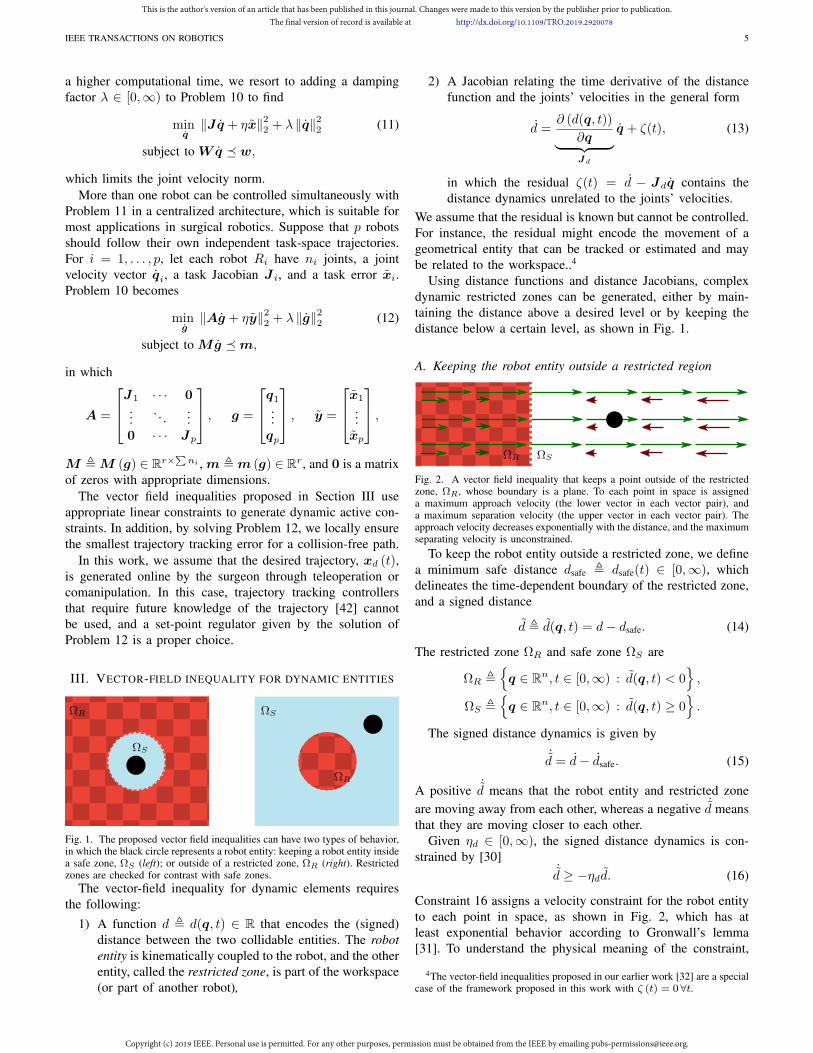
Fig. 1. The proposed vector field inequalities can have two types of behavior,in which the black circle represents a robot entity: keeping a robot entity insidea safe zone, ΩS (left); or outside of a restricted zone, ΩR (right). Restrictedzones are checked for contrast with safe zones.
The vector-field inequality for dynamic elements requires
the following:
1) A function d , d(q, t) ∈ R that encodes the (signed)
distance between the two collidable entities. The robot
entity is kinematically coupled to the robot, and the other
entity, called the restricted zone, is part of the workspace
(or part of another robot),
2) A Jacobian relating the time derivative of the distance
function and the joints’ velocities in the general form
d =∂ (d(q, t))
∂q︸ ︷︷ ︸
Jd
q + ζ(t), (13)
in which the residual ζ(t) = d − Jdq contains the
distance dynamics unrelated to the joints’ velocities.
We assume that the residual is known but cannot be controlled.
For instance, the residual might encode the movement of a
geometrical entity that can be tracked or estimated and may
be related to the workspace..4
Using distance functions and distance Jacobians, complex
dynamic restricted zones can be generated, either by main-
taining the distance above a desired level or by keeping the
distance below a certain level, as shown in Fig. 1.
A. Keeping the robot entity outside a restricted region
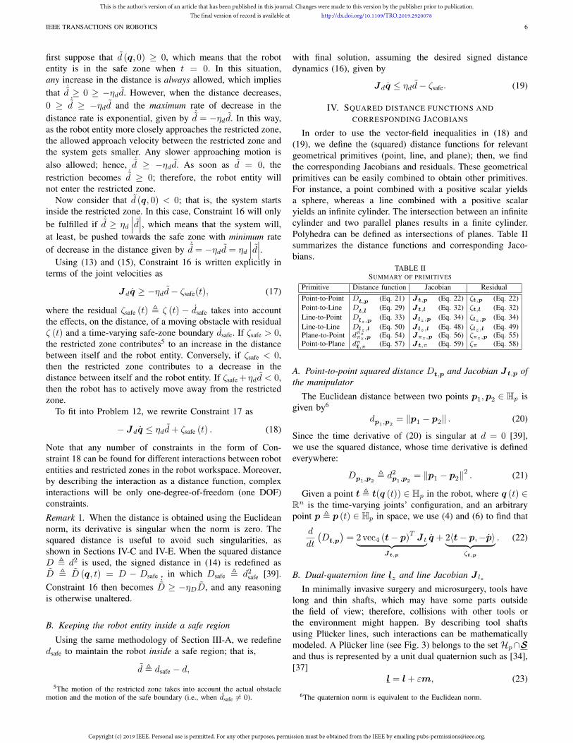
ΩR ΩS
Fig. 2. A vector field inequality that keeps a point outside of the restrictedzone, ΩR, whose boundary is a plane. To each point in space is assigneda maximum approach velocity (the lower vector in each vector pair), anda maximum separation velocity (the upper vector in each vector pair). Theapproach velocity decreases exponentially with the distance, and the maximumseparating velocity is unconstrained.
To keep the robot entity outside a restricted zone, we define
a minimum safe distance dsafe , dsafe(t) ∈ [0,∞), which
delineates the time-dependent boundary of the restricted zone,
and a signed distance
d , d(q, t) = d− dsafe. (14)
The restricted zone ΩR and safe zone ΩS are
ΩR ,
q ∈ Rn, t ∈ [0,∞) : d(q, t) < 0
,
ΩS ,
q ∈ Rn, t ∈ [0,∞) : d(q, t) ≥ 0
.
The signed distance dynamics is given by
˙d = d− dsafe. (15)
A positive˙d means that the robot entity and restricted zone
are moving away from each other, whereas a negative˙d means
that they are moving closer to each other.
Given ηd ∈ [0,∞), the signed distance dynamics is con-
strained by [30]˙d ≥ −ηdd. (16)
Constraint 16 assigns a velocity constraint for the robot entity
to each point in space, as shown in Fig. 2, which has at
least exponential behavior according to Gronwall’s lemma
[31]. To understand the physical meaning of the constraint,
4The vector-field inequalities proposed in our earlier work [32] are a specialcase of the framework proposed in this work with ζ (t) = 0 ∀t.
This is the author's version of an article that has been published in this journal. Changes were made to this version by the publisher prior to publication.The final version of record is available at http://dx.doi.org/10.1109/TRO.2019.2920078
Copyright (c) 2019 IEEE. Personal use is permitted. For any other purposes, permission must be obtained from the IEEE by emailing [email protected].
IEEE TRANSACTIONS ON ROBOTICS 6
first suppose that d (q, 0) ≥ 0, which means that the robot
entity is in the safe zone when t = 0. In this situation,
any increase in the distance is always allowed, which implies
that˙d ≥ 0 ≥ −ηdd. However, when the distance decreases,
0 ≥˙d ≥ −ηdd and the maximum rate of decrease in the
distance rate is exponential, given by˙d = −ηdd. In this way,
as the robot entity more closely approaches the restricted zone,
the allowed approach velocity between the restricted zone and
the system gets smaller. Any slower approaching motion is
also allowed; hence,˙d ≥ −ηdd. As soon as d = 0, the
restriction becomes˙d ≥ 0; therefore, the robot entity will
not enter the restricted zone.
Now consider that d (q, 0) < 0; that is, the system starts
inside the restricted zone. In this case, Constraint 16 will only
be fulfilled if˙d ≥ ηd
∣∣∣d∣∣∣, which means that the system will,
at least, be pushed towards the safe zone with minimum rate
of decrease in the distance given by˙d = −ηdd = ηd
∣∣∣d∣∣∣.
Using (13) and (15), Constraint 16 is written explicitly in
terms of the joint velocities as
Jdq ≥ −ηdd− ζsafe(t), (17)
where the residual ζsafe (t) , ζ (t) − dsafe takes into account
the effects, on the distance, of a moving obstacle with residual
ζ (t) and a time-varying safe-zone boundary dsafe. If ζsafe > 0,
the restricted zone contributes5 to an increase in the distance
between itself and the robot entity. Conversely, if ζsafe < 0,
then the restricted zone contributes to a decrease in the
distance between itself and the robot entity. If ζsafe +ηdd < 0,
then the robot has to actively move away from the restricted
zone.
To fit into Problem 12, we rewrite Constraint 17 as
− Jdq ≤ ηdd+ ζsafe (t) . (18)
Note that any number of constraints in the form of Con-
straint 18 can be found for different interactions between robot
entities and restricted zones in the robot workspace. Moreover,
by describing the interaction as a distance function, complex
interactions will be only one-degree-of-freedom (one DOF)
constraints.
Remark 1. When the distance is obtained using the Euclidean
norm, its derivative is singular when the norm is zero. The
squared distance is useful to avoid such singularities, as
shown in Sections IV-C and IV-E. When the squared distance
D , d2 is used, the signed distance in (14) is redefined as
D , D (q, t) = D − Dsafe , in which Dsafe , d2safe [39].
Constraint 16 then becomes˙D ≥ −ηDD, and any reasoning
is otherwise unaltered.
B. Keeping the robot entity inside a safe region
Using the same methodology of Section III-A, we redefine
dsafe to maintain the robot inside a safe region; that is,
d , dsafe − d,
5The motion of the restricted zone takes into account the actual obstaclemotion and the motion of the safe boundary (i.e., when dsafe 6= 0).
with final solution, assuming the desired signed distance
dynamics (16), given by
Jdq ≤ ηdd− ζsafe. (19)
IV. SQUARED DISTANCE FUNCTIONS AND
CORRESPONDING JACOBIANS
In order to use the vector-field inequalities in (18) and
(19), we define the (squared) distance functions for relevant
geometrical primitives (point, line, and plane); then, we find
the corresponding Jacobians and residuals. These geometrical
primitives can be easily combined to obtain other primitives.
For instance, a point combined with a positive scalar yields
a sphere, whereas a line combined with a positive scalar
yields an infinite cylinder. The intersection between an infinite
cylinder and two parallel planes results in a finite cylinder.
Polyhedra can be defined as intersections of planes. Table II
summarizes the distance functions and corresponding Jaco-
bians.
TABLE IISUMMARY OF PRIMITIVES
Primitive Distance function Jacobian Residual
Point-to-Point Dt,p (Eq. 21) Jt,p (Eq. 22) ζt,p (Eq. 22)
Point-to-Line Dt,l
(Eq. 29) Jt,l (Eq. 32) ζt,l (Eq. 32)
Line-to-Point Dlz ,p
(Eq. 33) Jlz ,p (Eq. 34) ζlz ,p (Eq. 34)
Line-to-Line Dlz ,l (Eq. 50) Jlz ,l (Eq. 48) ζlz ,l (Eq. 49)Plane-to-Point d
πzπz ,p (Eq. 54) Jπz ,p (Eq. 56) ζπz ,p (Eq. 55)
Point-to-Plane dπt,π (Eq. 57) Jt,π (Eq. 59) ζπ (Eq. 58)
A. Point-to-point squared distance Dt,p and Jacobian Jt,p of
the manipulator
The Euclidean distance between two points p1,p2 ∈ Hp is
given by6
dp1,p
2= ‖p1 − p2‖ . (20)
Since the time derivative of (20) is singular at d = 0 [39],
we use the squared distance, whose time derivative is defined
everywhere:
Dp1,p
2, d2p
1,p
2= ‖p1 − p2‖
2. (21)
Given a point t , t(q (t)) ∈ Hp in the robot, where q (t) ∈R
n is the time-varying joints’ configuration, and an arbitrary
point p , p (t) ∈ Hp in space, we use (4) and (6) to find that
d
dt
(Dt,p
)= 2vec4 (t− p)
TJ t
︸ ︷︷ ︸
Jt,p
q + 2〈t− p,−p〉︸ ︷︷ ︸
ζt,p
. (22)
B. Dual-quaternion line lz and line Jacobian J lz
In minimally invasive surgery and microsurgery, tools have
long and thin shafts, which may have some parts outside
the field of view; therefore, collisions with other tools or
the environment might happen. By describing tool shafts
using Plücker lines, such interactions can be mathematically
modeled. A Plücker line (see Fig. 3) belongs to the set Hp∩S
and thus is represented by a unit dual quaternion such as [34],
[37]
l = l+ εm, (23)
6The quaternion norm is equivalent to the Euclidean norm.
This is the author's version of an article that has been published in this journal. Changes were made to this version by the publisher prior to publication.The final version of record is available at http://dx.doi.org/10.1109/TRO.2019.2920078
Copyright (c) 2019 IEEE. Personal use is permitted. For any other purposes, permission must be obtained from the IEEE by emailing [email protected].
IEEE TRANSACTIONS ON ROBOTICS 7
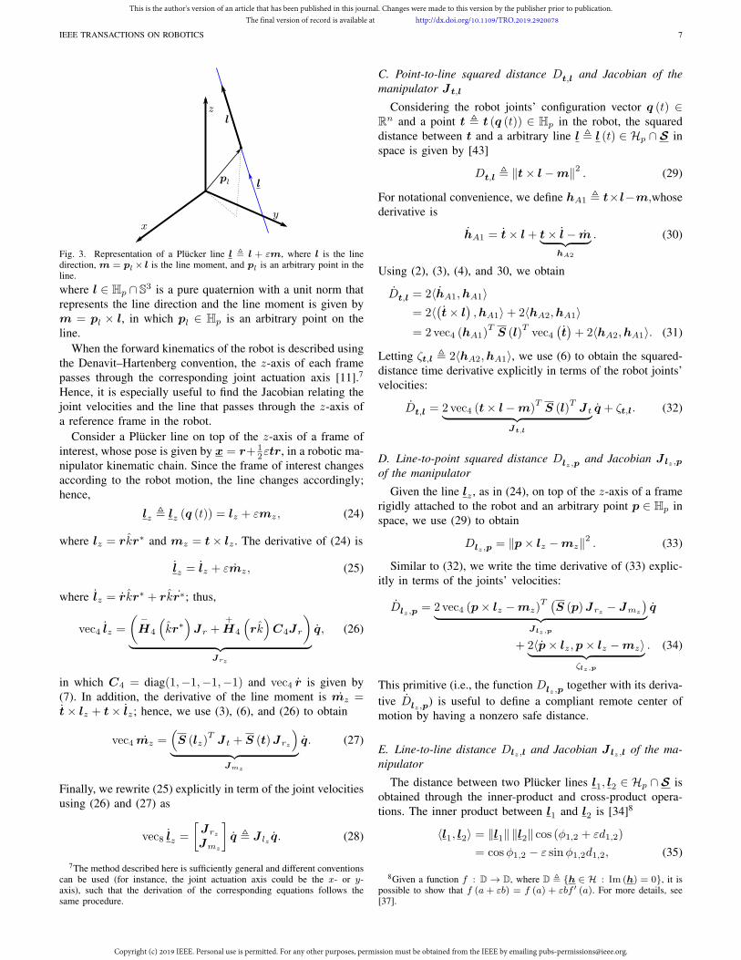
pl l
z
xy
l
Fig. 3. Representation of a Plücker line l , l + εm, where l is the linedirection, m = pl× l is the line moment, and pl is an arbitrary point in theline.
where l ∈ Hp ∩ S3 is a pure quaternion with a unit norm that
represents the line direction and the line moment is given by
m = pl × l, in which pl ∈ Hp is an arbitrary point on the
line.
When the forward kinematics of the robot is described using
the Denavit–Hartenberg convention, the z-axis of each frame
passes through the corresponding joint actuation axis [11].7
Hence, it is especially useful to find the Jacobian relating the
joint velocities and the line that passes through the z-axis of
a reference frame in the robot.
Consider a Plücker line on top of the z-axis of a frame of
interest, whose pose is given by x = r+ 12εtr, in a robotic ma-
nipulator kinematic chain. Since the frame of interest changes
according to the robot motion, the line changes accordingly;
hence,
lz , lz (q (t)) = lz + εmz, (24)
where lz = rkr∗ and mz = t× lz . The derivative of (24) is
lz = lz + εmz, (25)
where lz = rkr∗ + rkr∗; thus,
vec4 lz =
(−
H4
(
kr∗)
Jr ++
H4
(
rk)
C4Jr
)
︸ ︷︷ ︸
Jrz
q, (26)
in which C4 = diag(1,−1,−1,−1) and vec4 r is given by
(7). In addition, the derivative of the line moment is mz =t× lz + t× lz; hence, we use (3), (6), and (26) to obtain
vec4 mz =(
S (lz)TJ t + S (t)Jrz
)
︸ ︷︷ ︸
Jmz
q. (27)
Finally, we rewrite (25) explicitly in term of the joint velocities
using (26) and (27) as
vec8 lz =
[Jrz
Jmz
]
q , J lz q. (28)
7The method described here is sufficiently general and different conventionscan be used (for instance, the joint actuation axis could be the x- or y-axis), such that the derivation of the corresponding equations follows thesame procedure.
C. Point-to-line squared distance Dt,l and Jacobian of the
manipulator Jt,l
Considering the robot joints’ configuration vector q (t) ∈R
n and a point t , t (q (t)) ∈ Hp in the robot, the squared
distance between t and a arbitrary line l , l (t) ∈ Hp ∩ S in
space is given by [43]
Dt,l , ‖t× l−m‖2. (29)
For notational convenience, we define hA1 , t×l−m,whose
derivative is
hA1 = t× l+ t× l− m︸ ︷︷ ︸
hA2
. (30)
Using (2), (3), (4), and 30, we obtain
Dt,l = 2〈hA1,hA1〉
= 2〈(t× l
),hA1〉+ 2〈hA2,hA1〉
= 2vec4 (hA1)TS (l)
Tvec4
(t)+ 2〈hA2,hA1〉. (31)
Letting ζt,l , 2〈hA2,hA1〉, we use (6) to obtain the squared-
distance time derivative explicitly in terms of the robot joints’
velocities:
Dt,l = 2vec4 (t× l−m)TS (l)
TJ t
︸ ︷︷ ︸
Jt,l
q + ζt,l. (32)
D. Line-to-point squared distance Dlz,pand Jacobian J lz,p
of the manipulator
Given the line lz , as in (24), on top of the z-axis of a frame
rigidly attached to the robot and an arbitrary point p ∈ Hp in
space, we use (29) to obtain
Dlz,p= ‖p× lz −mz‖
2. (33)
Similar to (32), we write the time derivative of (33) explic-
itly in terms of the joints’ velocities:
Dlz,p= 2vec4 (p× lz −mz)
T (S (p)Jrz − Jmz
)
︸ ︷︷ ︸
Jlz,p
q
+ 2〈p× lz,p× lz −mz〉︸ ︷︷ ︸
ζlz,p
. (34)
This primitive (i.e., the function Dlz,ptogether with its deriva-
tive Dlz,p) is useful to define a compliant remote center of
motion by having a nonzero safe distance.
E. Line-to-line distance Dlz,l and Jacobian J lz,l of the ma-
nipulator
The distance between two Plücker lines l1, l2 ∈ Hp ∩ S is
obtained through the inner-product and cross-product opera-
tions. The inner product between l1 and l2 is [34]8
〈l1, l2〉 = ‖l1‖ ‖l2‖ cos (φ1,2 + εd1,2)
= cosφ1,2 − ε sinφ1,2d1,2, (35)
8Given a function f : D→ D, where D , h ∈ H : Im (h) = 0, it ispossible to show that f (a+ εb) = f (a) + εbf ′ (a). For more details, see[37].
This is the author's version of an article that has been published in this journal. Changes were made to this version by the publisher prior to publication.The final version of record is available at http://dx.doi.org/10.1109/TRO.2019.2920078
Copyright (c) 2019 IEEE. Personal use is permitted. For any other purposes, permission must be obtained from the IEEE by emailing [email protected].
IEEE TRANSACTIONS ON ROBOTICS 8
where d1,2 ∈ [0,∞) and φ1,2 ∈ [0, 2π) are the distance and
the angle between l1 and l2, respectively. Moreover, given
s1,2 ∈ Hp∩S—the line perpendicular to both l1 and l2—such
that s1,2 , s1,2 + εms1,2 , the cross product between l1 and
l2 is [34]
l1 × l2 = ‖l1‖ ‖l2‖ s1,2 sin (φ1,2 + εd1,2)
=(s1,2 + εms1,2
)(sinφ1,2 + ε cosφ1,2d1,2)
= s1,2 sinφ1,2+ε(ms1,2 sinφ1,2+s1,2 cosφ1,2d1,2
).
(36)
The squared distance between l1 and l2 when they are not
parallel (i.e., φ1,2 ∈ (0, 2π) \ π) is obtained using (35) and
(36):
D1,26‖ =‖D (〈l1, l2〉)‖
2
‖P (l1 × l2)‖2 =
‖d1,2 sinφ1,2‖2
‖s1,2 sinφ1,2‖2 = d21,2, (37)
The squared distance between l1 and l2 when they are parallel
(i.e., φ1,2 ∈ 0, π) is obtained as
D1,2‖ , ‖D (l1 × l2)‖2= ‖s1,2d1,2‖
2= d21,2. (38)
To find the distance Jacobian and residual between a line lzin the robot and an arbitrary line l in space, we begin by find-
ing the inner-product Jacobian and residual in Section IV-E1
and the cross product Jacobian and residual in Section IV-E2.
Those are used in Section IV-E3 to find the derivative of (37),
and in Section IV-E4 to find the derivative of (38). Finally,
they are unified in the final form of the distance Jacobian and
residual in Section IV-E5.
1) Inner-product Jacobian, J 〈lz,l〉: The time derivative of
the inner product between lz, l ∈ Hp ∩ S is given by
d
dt(〈lz, l〉) = 〈lz, l〉+ 〈lz, l〉 = −
1
2
(
lzl+ llz
)
+ 〈lz, l〉︸ ︷︷ ︸
ζ〈lz,l〉
.
Hence, using (28) we obtain
vec8d
dt(〈lz, l〉)=
J〈lz,l〉
︷ ︸︸ ︷
−1
2
(−
H8 (l)++
H8 (l)
)
J lz q+vec8 ζ〈lz,l〉,
which can be explicitly written in terms of the primary and
dual parts as
[vec4 P (〈lz, l〉)
vec4 D (〈lz, l〉)
]
=
[JP(〈lz,l〉)JD(〈lz,l〉)
]
q +
vec4 P
(
ζ〈lz,l〉
)
vec4 D(
ζ〈lz,l〉
)
.
(39)
2) Cross-product Jacobian, J lz×l: The time derivative of
the cross product between lz, l ∈ Hp ∩ S is given by
d
dt(lz × l) = lz × l+ lz × l =
1
2
(
lzl− llz
)
+ lz × l︸ ︷︷ ︸
ζlz×l
.
Using (28), we obtain
vec8d
dt(lz × l)=
Jlz×l
︷ ︸︸ ︷
1
2
(−
H8 (l)−+
H8 (l)
)
J lz q+vec8 ζlz×l,
which can be explicitly written in terms of the primary and
dual parts as
[vec4 P (lz × l)
vec4 D (lz × l)
]
=
[JP(lz×l)JD(lz×l)
]
q +
vec4 P
(
ζlz×l
)
vec4 D(
ζlz×l
)
(40)
3) Nonparallel distance Jacobian, J lz,l 6‖: From (37), the
squared distance between two nonparallel lines lz, l ∈ Hp∩S
is
Dlz,l 6‖ =‖D (〈lz, l〉)‖
2
‖P (lz × l)‖2 , (41)
with time derivative given by
Dlz,l 6‖ =
a︷ ︸︸ ︷
1
‖P (lz × l)‖2
d
dt
(
‖D (〈lz, l〉)‖2)
−‖D (〈lz, l〉)‖
2
‖P (lz × l)‖4
︸ ︷︷ ︸
b
d
dt
(
‖P (lz × l)‖2)
. (42)
We use (4) and (39) to obtain
d
dt
(
‖D (〈lz, l〉)‖2)
=
J‖D(〈lz,l〉)‖2
︷ ︸︸ ︷
2 vec4 D (〈lz, l〉)TJD(〈lz,l〉)
q
+ 2vec4 D (〈lz, l〉)Tvec4 D
(
ζ〈lz,l〉
)
︸ ︷︷ ︸
ζ‖D(〈lz,l〉)‖2
. (43)
Similarly, we use (4) and (40) to obtain
d
dt
(
‖P (lz × l)‖2)
=
J‖P(lz×l)‖2
︷ ︸︸ ︷
2 vec4 P (lz × l)TJP(lz×l)q
+ 2vec4 P (lz × l)Tvec4 P
(
ζlz×l
)
︸ ︷︷ ︸
ζ‖P(lz×l)‖2
. (44)
Finally, replacing (43) and (44) in (42) yields
Dlz,l 6‖ =
Jlz,l 6‖
︷ ︸︸ ︷(
aJ‖D(〈lz,l〉)‖2 + bJ‖P(lz×l)‖
2
)
q
+ aζ‖D(〈lz,l〉)‖
2 + bζ‖P(lz×l)‖
2
︸ ︷︷ ︸
ζlz,l 6‖
. (45)
4) Parallel distance Jacobian, J lz,l‖: In the degenerate
case where lz and l are parallel, the squared distance Dlz,l‖
is given by (38); that is,
Dlz,l‖= ‖D (lz × l)‖
2. (46)
Using (4) and (40), the derivative of (46) is given by
Dlz,l‖=
Jlz,l‖
︷ ︸︸ ︷
2 vec4 (D (lz × l))TJD(lz×l)q
+ 2vec4 (D (lz × l))Tvec4 D
(
ζlz×l
)
︸ ︷︷ ︸
ζlz,l‖
. (47)
This is the author's version of an article that has been published in this journal. Changes were made to this version by the publisher prior to publication.The final version of record is available at http://dx.doi.org/10.1109/TRO.2019.2920078
Copyright (c) 2019 IEEE. Personal use is permitted. For any other purposes, permission must be obtained from the IEEE by emailing [email protected].
IEEE TRANSACTIONS ON ROBOTICS 9
5) Line-to-line distance Jacobian, J lz,l of the manipulator:
The line-to-line distance Jacobian and residual are given by
taking into account both (45) and (47) as
J lz,l =
J lz,l 6‖ φ ∈ (0, 2π) \ π
J lz,l‖ φ ∈ 0, π, (48)
ζlz,l =
ζlz,l 6‖ φ ∈ (0, 2π) \ π
ζlz,l‖ φ ∈ 0, π, (49)
in which φ = arccosP (〈l, lz〉).Similarly, the distance between lines is given by taking into
account both (41) and (46) as
Dlz,l =
Dlz,l 6‖ φ ∈ (0, 2π) \ π
Dlz,l‖ φ ∈ 0, π. (50)
F. Plane-to-point distance dπzπz,p
and Jacobian Jπz,p of the
manipulator
pπ
nπ
dπ
π
z
x
y
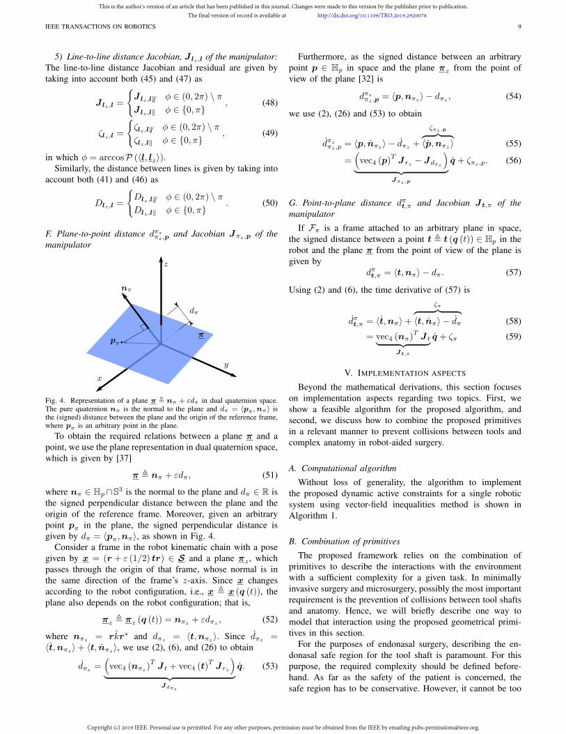
Fig. 4. Representation of a plane π , nπ + εdπ in dual quaternion space.The pure quaternion nπ is the normal to the plane and dπ = 〈pπ ,nπ〉 isthe (signed) distance between the plane and the origin of the reference frame,where pπ is an arbitrary point in the plane.
To obtain the required relations between a plane π and a
point, we use the plane representation in dual quaternion space,
which is given by [37]
π , nπ + εdπ, (51)
where nπ ∈ Hp∩S3 is the normal to the plane and dπ ∈ R is
the signed perpendicular distance between the plane and the
origin of the reference frame. Moreover, given an arbitrary
point pπ in the plane, the signed perpendicular distance is
given by dπ = 〈pπ,nπ〉, as shown in Fig. 4.
Consider a frame in the robot kinematic chain with a pose
given by x = (r + ε (1/2) tr) ∈ S and a plane πz , which
passes through the origin of that frame, whose normal is in
the same direction of the frame’s z-axis. Since x changes
according to the robot configuration, i.e., x , x (q (t)), the
plane also depends on the robot configuration; that is,
πz , πz (q (t)) = nπz+ εdπz
, (52)
where nπz= rkr∗ and dπz
= 〈t,nπz〉. Since dπz
=〈t,nπz
〉+ 〈t, nπz〉, we use (2), (6), and (26) to obtain
dπz=
(
vec4 (nπz)TJ t + vec4 (t)
TJrz
)
︸ ︷︷ ︸
Jdπz
q. (53)
Furthermore, as the signed distance between an arbitrary
point p ∈ Hp in space and the plane πz from the point of
view of the plane [32] is
dπzπz,p
= 〈p,nπz〉 − dπz
, (54)
we use (2), (26) and (53) to obtain
dπzπz,p
= 〈p, nπz〉 − dπz
+
ζπz,p
︷ ︸︸ ︷
〈p,nπz〉 (55)
=(
vec4 (p)TJrz − Jdπz
)
︸ ︷︷ ︸
Jπz,p
q + ζπz,p. (56)
G. Point-to-plane distance dπt,π and Jacobian Jt,π of the
manipulator
If Fπ is a frame attached to an arbitrary plane in space,
the signed distance between a point t , t (q (t)) ∈ Hp in the
robot and the plane π from the point of view of the plane is
given by
dπt,π = 〈t,nπ〉 − dπ. (57)
Using (2) and (6), the time derivative of (57) is
dπt,π = 〈t,nπ〉+
ζπ︷ ︸︸ ︷
〈t, nπ〉 − dπ (58)
= vec4 (nπ)TJ t
︸ ︷︷ ︸
Jt,π
q + ζπ (59)
V. IMPLEMENTATION ASPECTS
Beyond the mathematical derivations, this section focuses
on implementation aspects regarding two topics. First, we
show a feasible algorithm for the proposed algorithm, and
second, we discuss how to combine the proposed primitives
in a relevant manner to prevent collisions between tools and
complex anatomy in robot-aided surgery.
A. Computational algorithm
Without loss of generality, the algorithm to implement
the proposed dynamic active constraints for a single robotic
system using vector-field inequalities method is shown in
Algorithm 1.
B. Combination of primitives
The proposed framework relies on the combination of
primitives to describe the interactions with the environment
with a sufficient complexity for a given task. In minimally
invasive surgery and microsurgery, possibly the most important
requirement is the prevention of collisions between tool shafts
and anatomy. Hence, we will briefly describe one way to
model that interaction using the proposed geometrical primi-
tives in this section.
For the purposes of endonasal surgery, describing the en-
donasal safe region for the tool shaft is paramount. For this
purpose, the required complexity should be defined before-
hand. As far as the safety of the patient is concerned, the
safe region has to be conservative. However, it cannot be too
This is the author's version of an article that has been published in this journal. Changes were made to this version by the publisher prior to publication.The final version of record is available at http://dx.doi.org/10.1109/TRO.2019.2920078
Copyright (c) 2019 IEEE. Personal use is permitted. For any other purposes, permission must be obtained from the IEEE by emailing [email protected].
IEEE TRANSACTIONS ON ROBOTICS 10
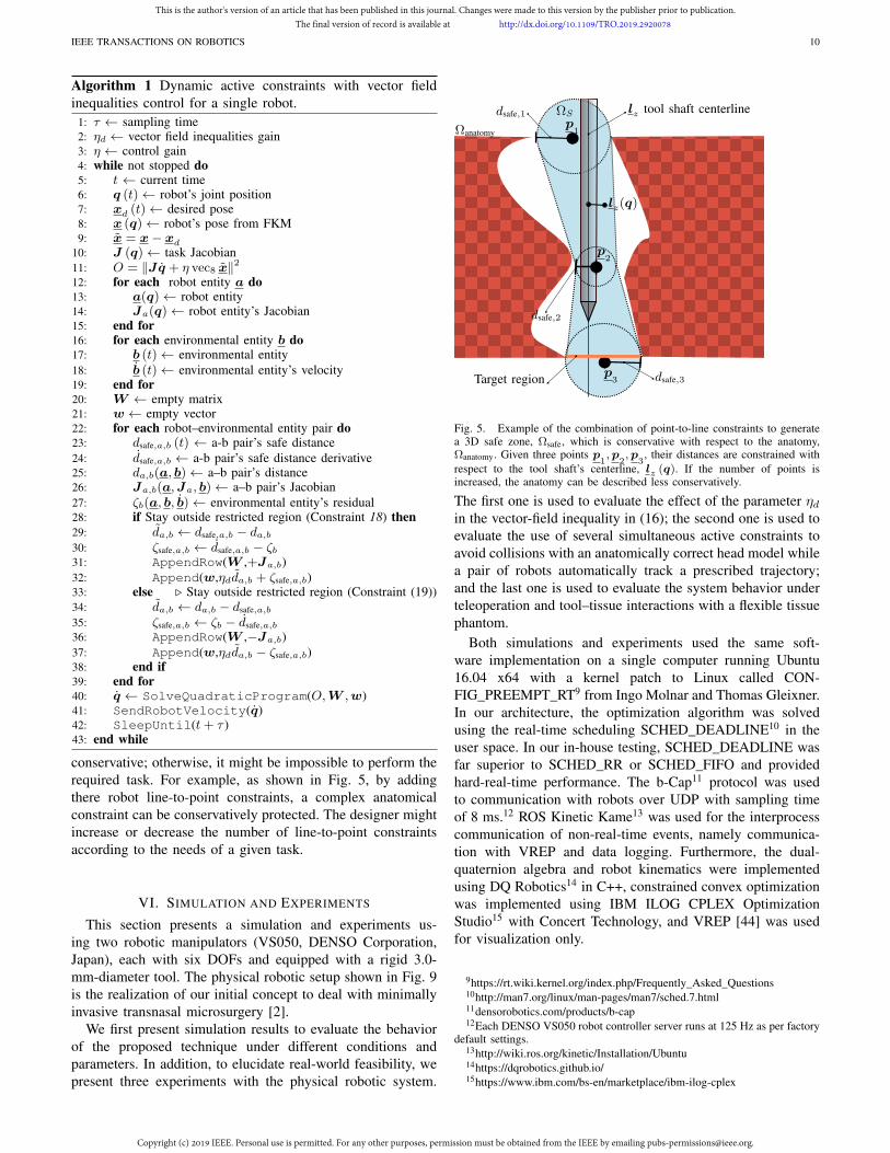
Algorithm 1 Dynamic active constraints with vector field
inequalities control for a single robot.
1: τ ← sampling time2: ηd ← vector field inequalities gain3: η ← control gain4: while not stopped do5: t ← current time6: q (t)← robot’s joint position7: xd (t)← desired pose8: x (q)← robot’s pose from FKM9: x = x− xd
10: J (q)← task Jacobian
11: O = ‖Jq + η vec8 x‖2
12: for each robot entity a do13: a(q)← robot entity14: Ja(q)← robot entity’s Jacobian15: end for16: for each environmental entity b do17: b (t)← environmental entity
18: b (t)← environmental entity’s velocity19: end for20: W ← empty matrix21: w ← empty vector22: for each robot–environmental entity pair do23: dsafe,a,b (t) ← a-b pair’s safe distance
24: dsafe,a,b ← a-b pair’s safe distance derivative25: da,b(a, b)← a–b pair’s distance26: Ja,b(a,Ja, b)← a–b pair’s Jacobian
27: ζb(a, b, b)← environmental entity’s residual28: if Stay outside restricted region (Constraint 18) then
29: da,b ← dsafe,a,b − da,b30: ζsafe,a,b ← dsafe,a,b − ζb31: AppendRow(W ,+Ja,b)
32: Append(w,ηdda,b + ζsafe,a,b)33: else ⊲ Stay outside restricted region (Constraint (19))
34: da,b ← da,b − dsafe,a,b
35: ζsafe,a,b ← ζb − dsafe,a,b
36: AppendRow(W ,−Ja,b)
37: Append(w,ηdda,b − ζsafe,a,b)38: end if39: end for40: q ← SolveQuadraticProgram(O,W ,w)41: SendRobotVelocity(q)42: SleepUntil(t+ τ )43: end while
conservative; otherwise, it might be impossible to perform the
required task. For example, as shown in Fig. 5, by adding
there robot line-to-point constraints, a complex anatomical
constraint can be conservatively protected. The designer might
increase or decrease the number of line-to-point constraints
according to the needs of a given task.
VI. SIMULATION AND EXPERIMENTS
This section presents a simulation and experiments us-
ing two robotic manipulators (VS050, DENSO Corporation,
Japan), each with six DOFs and equipped with a rigid 3.0-
mm-diameter tool. The physical robotic setup shown in Fig. 9
is the realization of our initial concept to deal with minimally
invasive transnasal microsurgery [2].
We first present simulation results to evaluate the behavior
of the proposed technique under different conditions and
parameters. In addition, to elucidate real-world feasibility, we
present three experiments with the physical robotic system.
dsafe,1
p2
lz(q)
dsafe,3
dsafe,2
Ωanatomy
p3
p1
ΩS lz tool shaft centerline
Target region
Fig. 5. Example of the combination of point-to-line constraints to generatea 3D safe zone, Ωsafe, which is conservative with respect to the anatomy,Ωanatomy. Given three points p
1,p
2,p
3, their distances are constrained with
respect to the tool shaft’s centerline, lz (q). If the number of points isincreased, the anatomy can be described less conservatively.
The first one is used to evaluate the effect of the parameter ηdin the vector-field inequality in (16); the second one is used to
evaluate the use of several simultaneous active constraints to
avoid collisions with an anatomically correct head model while
a pair of robots automatically track a prescribed trajectory;
and the last one is used to evaluate the system behavior under
teleoperation and tool–tissue interactions with a flexible tissue
phantom.
Both simulations and experiments used the same soft-
ware implementation on a single computer running Ubuntu
16.04 x64 with a kernel patch to Linux called CON-
FIG_PREEMPT_RT9 from Ingo Molnar and Thomas Gleixner.
In our architecture, the optimization algorithm was solved
using the real-time scheduling SCHED_DEADLINE10 in the
user space. In our in-house testing, SCHED_DEADLINE was
far superior to SCHED_RR or SCHED_FIFO and provided
hard-real-time performance. The b-Cap11 protocol was used
to communication with robots over UDP with sampling time
of 8 ms.12 ROS Kinetic Kame13 was used for the interprocess
communication of non-real-time events, namely communica-
tion with VREP and data logging. Furthermore, the dual-
quaternion algebra and robot kinematics were implemented
using DQ Robotics14 in C++, constrained convex optimization
was implemented using IBM ILOG CPLEX Optimization
Studio15 with Concert Technology, and VREP [44] was used
for visualization only.
9https://rt.wiki.kernel.org/index.php/Frequently_Asked_Questions10http://man7.org/linux/man-pages/man7/sched.7.html11densorobotics.com/products/b-cap12Each DENSO VS050 robot controller server runs at 125 Hz as per factory
default settings.13http://wiki.ros.org/kinetic/Installation/Ubuntu14https://dqrobotics.github.io/15https://www.ibm.com/bs-en/marketplace/ibm-ilog-cplex
This is the author's version of an article that has been published in this journal. Changes were made to this version by the publisher prior to publication.The final version of record is available at http://dx.doi.org/10.1109/TRO.2019.2920078
Copyright (c) 2019 IEEE. Personal use is permitted. For any other purposes, permission must be obtained from the IEEE by emailing [email protected].
IEEE TRANSACTIONS ON ROBOTICS 11
In the experiments, the tool-tip position with respect to the
robot end effector was calibrated by using a visual tracking
system (Polaris Spectra, NDI, Canada) through a pivoting pro-
cess.16 The visual tracking system was also used to calibrate
one robot base with respect to the other.
A. Simulation: Shaft–shaft active constraint
In the first simulation, two robots (R1 and R2) were
positioned on opposite sides of the workspace. The robots
were initially positioned so that their tool shafts cross when
viewed from the xz-plane. Both robots were commanded to
simultaneously move their tools along the y-axis. The tools
first moved along the same trajectory along the negative y-
axis direction such that R1 followed R2 with a slight offset
during t ∈ [0, 2 s); then, both robots maintained simultaneous
motion but changed their direction along the y-axis so that R2
followed R1 during t ∈ [2 s, 4 s), moved toward each other
during t ∈ [4 s, 6 s), and finally moved away from each other
during t ∈ [6 s, 8 s]. The reference trajectory required the tool
orientations to remain constant. The tools were simulated as
3.0-mm-diameter cylindrical shafts.
In order to study the dynamic active constraint to prevent
collision a between shafts, we consider three different ways of
generating the control inputs. In the first one, the control input
is generated by the solution of Problem 8; therefore, as the
robot does not take into account any obstacle and is unaware
of its surroundings, we say it is oblivious. In the second and
third ones, the control input is generated by the solution of
Problem 10 with Constraint 18 and (48), (49), and (50). How-
ever, in the second one, the residual is not used; thus, it is a
static-aware robot. That is, the robot considers its surroundings
but does not take into account obstacle kinematics. In the third
one, a robot controlled with the full proposed dynamic active
constraints including the residual is called a kinematics-aware
robot. If both robots are kinematics-aware, the centralized
Problem 12 was used to solve for both robots simultaneously.
With these definitions, we examine every unique combination
of states between robots for a convergence rate η = 50,
an approach gain ηd ∈ 0, 1, 2, 3, 4, 5, 6, 7, 8.5, 10, and a
sampling time τ = 8 ms. A static-aware robot is what could
be achieved without using the proposed residuals; therefore, it
is equivalent to [32]. Hence, the results of these simulations
are appropriate to compare our initial results presented in [32]
to the ones reported in this paper.
The design parameter ηd corresponds to the fastest distance
decay allowed between two moving robotic systems; therefore,
in a system where both robots are kinematics-aware, have the
same approach gain ηd, and move directly towards each other,
the result of the optimization will assign a gain of ηd/2 for
each robot in the most restrictive case. Thus, to provide a fair
comparison in the same scenario, when both robots are static-
aware, the approach gain ηd was divided in half.
1) Results and discussion: The performance for ηd = 2 in
terms of the trajectory tracking error and minimum separation
16The pivoting process consists in adding a marker to the tool, then pivotingthe tool tip about a divot and recording the marker coordinates to obtain therelative translation between marker and tool tip. This process is available inthe manufacturer’s software.
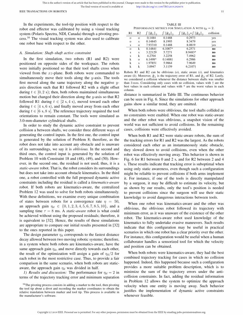
TABLE IIIPERFORMANCE METRICS FOR SIMULATION A WITH ηd = 2.
R1 R2∫‖x1‖2
∫‖x2‖2
∫‖x1‖2+
∫‖x2‖2 collision
o o 0.1484 0.1488 0.2973 yeso s 0.14845 8.1995 8.3479 yess o 7.93310 0.1488 8.0819 yes
o k 0.1484† 6.1087* 6.2571 no
s s 3.22129 5.7271 8.9483* no
s k 4.2704 3.2258 7.4962 no
k o 6.1498* 0.1488† 6.2986 no
k s 1.97851 5.9864 7.9649 no
k k 3.0947 3.1159 6.2107† no
Robots R1 and R2 can be oblivious (o), static aware (s), and kinematicsaware (k). Moreover, x1 is the trajectory error of R1, and x2 of R2. Lastly,we considered a collision whenever the distance between shafts was smallerthan 3mm. Considering only cases with no collision, values with † are thebest values in each column and values with * are the worst values in eachcolumn.
distance is summarized in Table III. The continuous behavior
can be seen in Fig. 6. Since the simulations for other approach
gains show a similar trend, they are omitted.
When both robots were oblivious, the tool shafts collided as
no constraints were enabled. When one robot was static-aware
and the other robot was oblivious, a snapshot vision of the
world was not sufficient to avoid collisions. In the remaining
cases, collisions were effectively avoided.
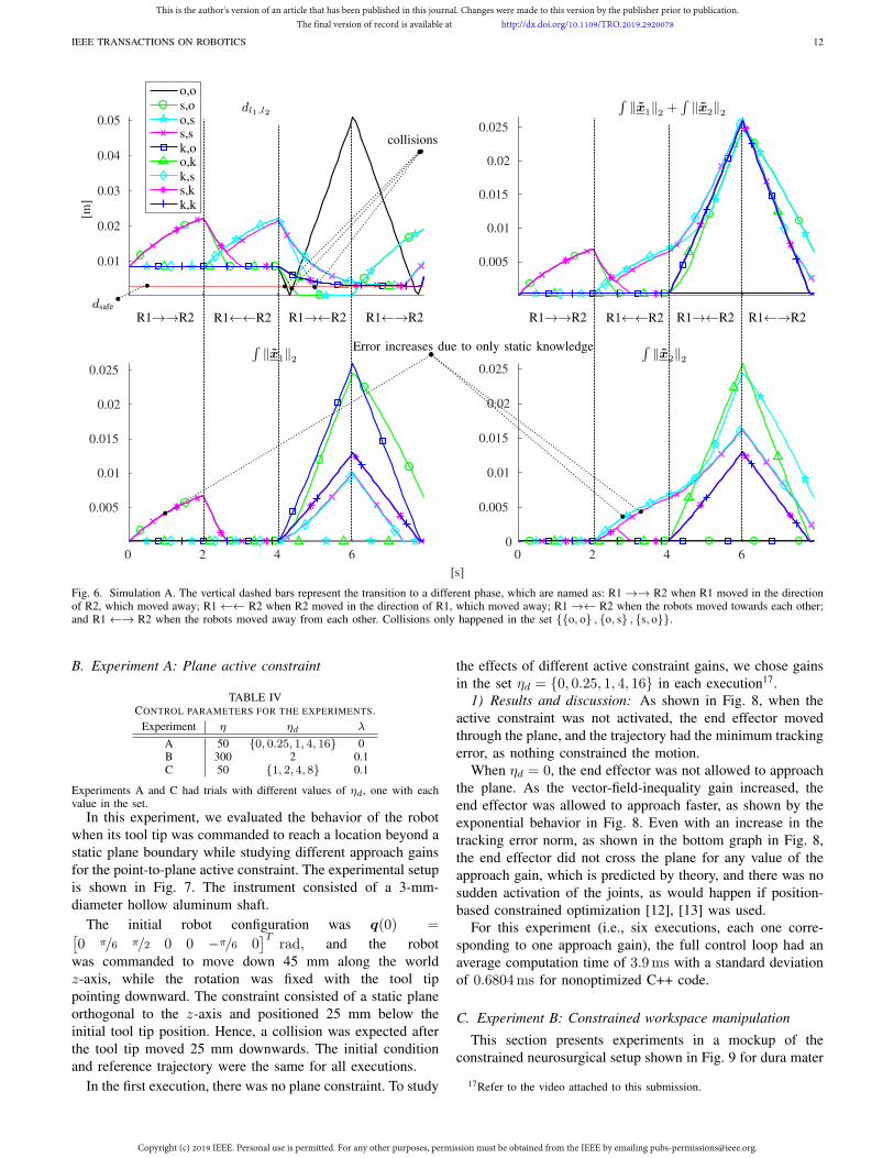
When both R1 and R2 were static-aware robots, the sum of
the tracking errors for R1 and R2 was the largest. As the robots
considered each other as an instantaneously static obstacle,
they slowed down to avoid collisions, even when the other
robot was effectively moving away. This behavior is shown in
Fig. 6 for R1 between 0 and 2 s, and for R2 between 2 and 4
s. These results indicate that tracking error is suboptimal when
using only static awareness, even though such a configuration
might be reliable to prevent collisions if both arms implement
it. For instance, if one of the tools is directly manipulated
by a surgeon, it may be difficult to estimate its velocity, but
as shown by our results, only the tool’s position is needed
to prevent collisions since the surgeon will use their static
knowledge to avoid dangerous interactions between tools.
When one robot was kinematics-aware and the other was
oblivious, the oblivious robot followed its trajectory with
minimum error, as it was unaware of the existence of the other
robot. The kinematics-aware robot used knowledge of the
kinematics to fully undertake evasive maneuvers. Such results
indicate that this configuration may be useful in practical
scenarios in which one robot has a clear priority over the other.
For instance, this configuration would be useful when a human
collaborator handles a sensorized tool for which the velocity
and position can be obtained.
When both robots were kinematics-aware, they had the best
combined trajectory tracking for cases in which no collision
happened. Indeed, this happened because such a configuration
provides a more suitable problem description, which is to
minimize the sum of the trajectory errors under the anti-
collision constraints. In fact, adding the residual information
in Problem 12 allows the system to optimize the approach
velocity when one entity is moving away. Such behavior
justifies the implementation of dynamic active constraints
whenever feasible.
This is the author's version of an article that has been published in this journal. Changes were made to this version by the publisher prior to publication.The final version of record is available at http://dx.doi.org/10.1109/TRO.2019.2920078
Copyright (c) 2019 IEEE. Personal use is permitted. For any other purposes, permission must be obtained from the IEEE by emailing [email protected].
IEEE TRANSACTIONS ON ROBOTICS 12
0.01
0.02
0.03
0.04
0.05
[m]
dl1,l2
0.005
0.01
0.015
0.02
0.025
∫‖x1‖2 +
∫‖x2‖2
0 2 4 6
[s]
0.005
0.01
0.015
0.02
0.025
∫‖x1‖2
0 2 4 60
0.005
0.01
0.015
0.02
0.025
∫‖x2‖2
o,os,oo,ss,sk,oo,kk,ss,kk,k
R1→→R2 R1←←R2 R1←→R2R1→←R2dsafe
collisions
Error increases due to only static knowledge
R1→→R2 R1←←R2 R1←→R2R1→←R2
Fig. 6. Simulation A. The vertical dashed bars represent the transition to a different phase, which are named as: R1→→ R2 when R1 moved in the directionof R2, which moved away; R1←← R2 when R2 moved in the direction of R1, which moved away; R1→← R2 when the robots moved towards each other;and R1←→ R2 when the robots moved away from each other. Collisions only happened in the set o, o , o, s , s, o.
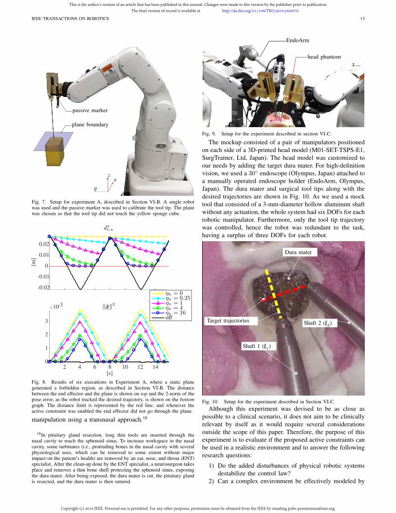
B. Experiment A: Plane active constraint
TABLE IVCONTROL PARAMETERS FOR THE EXPERIMENTS.
Experiment η ηd λ
A 50 0, 0.25, 1, 4, 16 0B 300 2 0.1C 50 1, 2, 4, 8 0.1
Experiments A and C had trials with different values of ηd, one with eachvalue in the set.
In this experiment, we evaluated the behavior of the robot
when its tool tip was commanded to reach a location beyond a
static plane boundary while studying different approach gains
for the point-to-plane active constraint. The experimental setup
is shown in Fig. 7. The instrument consisted of a 3-mm-
diameter hollow aluminum shaft.
The initial robot configuration was q(0) =[0 π/6 π/2 0 0 −π/6 0
]Trad, and the robot
was commanded to move down 45 mm along the world
z-axis, while the rotation was fixed with the tool tip
pointing downward. The constraint consisted of a static plane
orthogonal to the z-axis and positioned 25 mm below the
initial tool tip position. Hence, a collision was expected after
the tool tip moved 25 mm downwards. The initial condition
and reference trajectory were the same for all executions.
In the first execution, there was no plane constraint. To study
the effects of different active constraint gains, we chose gains
in the set ηd = 0, 0.25, 1, 4, 16 in each execution17.
1) Results and discussion: As shown in Fig. 8, when the
active constraint was not activated, the end effector moved
through the plane, and the trajectory had the minimum tracking
error, as nothing constrained the motion.
When ηd = 0, the end effector was not allowed to approach
the plane. As the vector-field-inequality gain increased, the
end effector was allowed to approach faster, as shown by the
exponential behavior in Fig. 8. Even with an increase in the
tracking error norm, as shown in the bottom graph in Fig. 8,
the end effector did not cross the plane for any value of the
approach gain, which is predicted by theory, and there was no
sudden activation of the joints, as would happen if position-
based constrained optimization [12], [13] was used.
For this experiment (i.e., six executions, each one corre-
sponding to one approach gain), the full control loop had an
average computation time of 3.9ms with a standard deviation
of 0.6804ms for nonoptimized C++ code.
C. Experiment B: Constrained workspace manipulation
This section presents experiments in a mockup of the
constrained neurosurgical setup shown in Fig. 9 for dura mater
17Refer to the video attached to this submission.
This is the author's version of an article that has been published in this journal. Changes were made to this version by the publisher prior to publication.The final version of record is available at http://dx.doi.org/10.1109/TRO.2019.2920078
Copyright (c) 2019 IEEE. Personal use is permitted. For any other purposes, permission must be obtained from the IEEE by emailing [email protected].
IEEE TRANSACTIONS ON ROBOTICS 13
plane boundary
passive marker
zx
y
Fig. 7. Setup for experiment A, described in Section VI-B. A single robotwas used and the passive marker was used to calibrate the tool tip. The planewas chosen so that the tool tip did not touch the yellow sponge cube.
-0.02
-0.01
0
0.01
0.02
[m]
dπt,π
2 4 6 8 10 12 14[s]
0
1
2
3
10-3 ‖x‖2
ηπ = 0ηπ = 0.25ηπ = 1ηπ = 4ηπ = 16off
Fig. 8. Results of six executions in Experiment A, where a static planegenerated a forbidden region, as described in Section VI-B. The distancebetween the end effector and the plane is shown on top and the 2-norm of thepose error, as the robot tracked the desired trajectory, is shown on the bottom
graph. The distance limit is represented by the red line, and whenever theactive constraint was enabled the end effector did not go through the plane.
manipulation using a transnasal approach.18
18In pituitary gland resection, long thin tools are inserted through thenasal cavity to reach the sphenoid sinus. To increase workspace in the nasalcavity, some turbinates (i.e., protruding bones in the nasal cavity with severalphysiological uses, which can be removed to some extent without majorimpact on the patient’s health) are removed by an ear, nose, and throat (ENT)specialist. After the clean-up done by the ENT specialist, a neurosurgeon takesplace and removes a thin bone shell protecting the sphenoid sinus, exposingthe dura mater. After being exposed, the dura mater is cut, the pituitary glandis resected, and the dura mater is then sutured.
EndoArm
head phantom
Fig. 9. Setup for the experiment described in section VI-C.
The mockup consisted of a pair of manipulators positioned
on each side of a 3D-printed head model (M01-SET-TSPS-E1,
SurgTrainer, Ltd, Japan). The head model was customized to
our needs by adding the target dura mater. For high-definition
vision, we used a 30 endoscope (Olympus, Japan) attached to
a manually operated endoscope holder (EndoArm, Olympus,
Japan). The dura mater and surgical tool tips along with the
desired trajectories are shown in Fig. 10. As we used a mock
tool that consisted of a 3-mm-diameter hollow aluminum shaft
without any actuation, the whole system had six DOFs for each
robotic manipulator. Furthermore, only the tool tip trajectory
was controlled, hence the robot was redundant to the task,
having a surplus of three DOFs for each robot.
Target trajectories
Dura mater
Shaft 1 (l1)
Shaft 2 (l2)
Fig. 10. Setup for the experiment described in Section VI-C.
Although this experiment was devised to be as close as
possible to a clinical scenario, it does not aim to be clinically
relevant by itself as it would require several considerations
outside the scope of this paper. Therefore, the purpose of this
experiment is to evaluate if the proposed active constraints can
be used in a realistic environment and to answer the following
research questions:
1) Do the added disturbances of physical robotic systems
destabilize the control law?
2) Can a complex environment be effectively modeled by
This is the author's version of an article that has been published in this journal. Changes were made to this version by the publisher prior to publication.The final version of record is available at http://dx.doi.org/10.1109/TRO.2019.2920078
Copyright (c) 2019 IEEE. Personal use is permitted. For any other purposes, permission must be obtained from the IEEE by emailing [email protected].
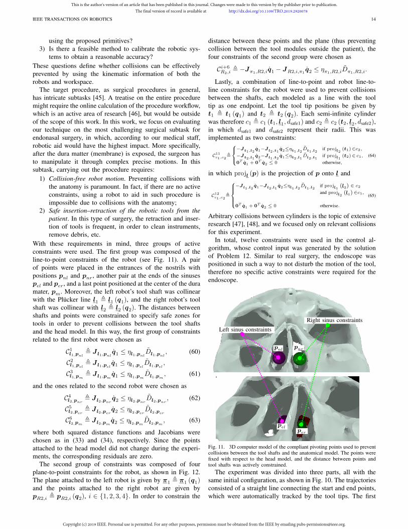
IEEE TRANSACTIONS ON ROBOTICS 14
using the proposed primitives?
3) Is there a feasible method to calibrate the robotic sys-
tems to obtain a reasonable accuracy?
These questions define whether collisions can be effectively
prevented by using the kinematic information of both the
robots and workspace.
The target procedure, as surgical procedures in general,
has intricate subtasks [45]. A treatise on the entire procedure
might require the online calculation of the procedure workflow,
which is an active area of research [46], but would be outside
of the scope of this work. In this work, we focus on evaluating
our technique on the most challenging surgical subtask for
endonasal surgery, in which, according to our medical staff,
robotic aid would have the highest impact. More specifically,
after the dura matter (membrane) is exposed, the surgeon has
to manipulate it through complex precise motions. In this
subtask, carrying out the procedure requires:
1) Collision-free robot motion. Preventing collisions with
the anatomy is paramount. In fact, if there are no active
constraints, using a robot to aid in such procedure is
impossible due to collisions with the anatomy;
2) Safe insertion–retraction of the robotic tools from the
patient. In this type of surgery, the retraction and inser-
tion of tools is frequent, in order to clean instruments,
remove debris, etc.
With these requirements in mind, three groups of active
constraints were used. The first group was composed of the
line-to-point constraints of the robot (see Fig. 11). A pair
of points were placed in the entrances of the nostrils with
positions pnl and pnr, another pair at the ends of the sinuses
pel and per, and a last point positioned at the center of the dura
mater, pm. Moreover, the left robot’s tool shaft was collinear
with the Plücker line l1 , l1 (q1), and the right robot’s tool
shaft was collinear with l2 , l2 (q2). The distances between
shafts and points were constrained to specify safe zones for
tools in order to prevent collisions between the tool shafts
and the head model. In this way, the first group of constraints
related to the first robot were chosen as
C1l1,pnl
, J l1,pnlq1 ≤ ηl1,pnl
Dl1,pnl, (60)
C2l1,pel
, J l1,pelq1 ≤ ηl1,pel
Dl1,pel,
C3l1,pm
, J l1,pmq1 ≤ ηl1,pm
Dl1,pm, (61)
and the ones related to the second robot were chosen as
C4l2,pnr
, J l2,pnrq2 ≤ ηl2,pnr
Dl2,pnr, (62)
C5l2,per
, J l2,perq2 ≤ ηl2,per
Dl2,per
C6l2,pm
, J l2,pmq2 ≤ ηl2,pm
Dl2,pm, (63)
where both squared distance functions and Jacobians were
chosen as in (33) and (34), respectively. Since the points
attached to the head model did not change during the experi-
ments, the corresponding residuals are zero.
The second group of constraints was composed of four
plane-to-point constraints for the robot, as shown in Fig. 12.
The plane attached to the left robot is given by π1 , π1 (q1)and the points attached to the right robot are given by
pR2,i , pR2,i (q2), i ∈ 1, 2, 3, 4. In order to constrain the
distance between these points and the plane (thus preventing
collision between the tool modules outside the patient), the
four constraints of the second group were chosen as
Ci+6R2,i
, −Jπ1,R2,iq1 − JR2,i,π1q2 ≤ ηπ1,R2,iDπ1,R2,i.
Lastly, a combination of line-to-point and robot line-to-
line constraints for the robot were used to prevent collisions
between the shafts, each modeled as a line with the tool
tip as one endpoint. Let the tool tip positions be given by
t1 , t1 (q1) and t2 , t2 (q2). Each semi-infinite cylinder
was therefore c1 , c1 (t1, l1, dsafe1) and c2 , c2 (t2, l2, dsafe2),in which dsafe1 and dsafe2 represent their radii. This was
implemented as two constraints:
C11
c1,c2,
−Jt1,l2q1−Jl2,t1
q2≤ηt1,l2
Dt1,l2if projl2
(t1)∈c2,
−Jt2,l1q2−Jl1,t2
q1≤ηt2,l1
Dl2,t1if projl1
(t2)∈ c1,
0T q
1+ 0
T q2≤ 0 otherwise,
(64)
in which projl (p) is the projection of p onto l and
C12
c1,c2,
−Jl1,l2q1−Jl2,l1
q2≤ηl1,l2
Dl1,l2if projl1
(
l2
)
∈ c2
and projl2
(
l1
)
∈c1,
0T q
1+ 0
T q2≤ 0 otherwise.
(65)
Arbitrary collisions between cylinders is the topic of extensive
research [47], [48], and we focused only on relevant collisions
for this experiment.
In total, twelve constraints were used in the control al-
gorithm, whose control input was generated by the solution
of Problem 12. Similar to real surgery, the endoscope was
positioned in such a way to not disturb the motion of the tool,
therefore no specific active constraints were required for the
endoscope.
Left sinus constraints
Right sinus constraints
pnlpnr
pelper
Fig. 11. 3D computer model of the compliant pivoting points used to preventcollisions between the tool shafts and the anatomical model. The points werefixed with respect to the head model, and the distance between points andtool shafts was actively constrained.
The experiment was divided into three parts, all with the
same initial configuration, as shown in Fig. 10. The trajectories
consisted of a straight line connecting the start and end points,
which were automatically tracked by the tool tips. The first
This is the author's version of an article that has been published in this journal. Changes were made to this version by the publisher prior to publication.The final version of record is available at http://dx.doi.org/10.1109/TRO.2019.2920078
Copyright (c) 2019 IEEE. Personal use is permitted. For any other purposes, permission must be obtained from the IEEE by emailing [email protected].
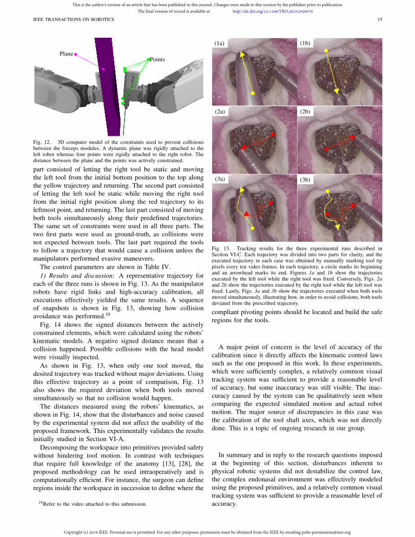
IEEE TRANSACTIONS ON ROBOTICS 15
PointsPlane
Fig. 12. 3D computer model of the constraints used to prevent collisionsbetween the forceps modules. A dynamic plane was rigidly attached to theleft robot whereas four points were rigidly attached to the right robot. Thedistance between the plane and the points was actively constrained.
part consisted of letting the right tool be static and moving
the left tool from the initial bottom position to the top along
the yellow trajectory and returning. The second part consisted
of letting the left tool be static while moving the right tool
from the initial right position along the red trajectory to its
leftmost point, and returning. The last part consisted of moving
both tools simultaneously along their predefined trajectories.
The same set of constraints were used in all three parts. The
two first parts were used as ground-truth, as collisions were
not expected between tools. The last part required the tools
to follow a trajectory that would cause a collision unless the
manipulators performed evasive maneuvers.
The control parameters are shown in Table IV.
1) Results and discussion: A representative trajectory for
each of the three runs is shown in Fig. 13. As the manipulator
robots have rigid links and high-accuracy calibration, all
executions effectively yielded the same results. A sequence
of snapshots is shown in Fig. 13, showing how collision
avoidance was performed.19
Fig. 14 shows the signed distances between the actively
constrained elements, which were calculated using the robots’
kinematic models. A negative signed distance means that a
collision happened. Possible collisions with the head model
were visually inspected.
As shown in Fig. 13, when only one tool moved, the
desired trajectory was tracked without major deviations. Using
this effective trajectory as a point of comparison, Fig. 13
also shows the required deviation when both tools moved
simultaneously so that no collision would happen.
The distances measured using the robots’ kinematics, as
shown in Fig. 14, show that the disturbances and noise caused
by the experimental system did not affect the usability of the
proposed framework. This experimentally validates the results
initially studied in Section VI-A.
Decomposing the workspace into primitives provided safety
without hindering tool motion. In contrast with techniques
that require full knowledge of the anatomy [13], [28], the
proposed methodology can be used intraoperatively and is
computationally efficient. For instance, the surgeon can define
regions inside the workspace in succession to define where the
19Refer to the video attached to this submission.
(1a) (1b)
(2a) (2b)
(3a) (3b)
Fig. 13. Tracking results for the three experimental runs described inSection VI-C. Each trajectory was divided into two parts for clarity, and theexecuted trajectory in each case was obtained by manually marking tool tippixels every ten video frames. In each trajectory, a circle marks its beginningand an arrowhead marks its end. Figures 1a and 1b show the trajectoriesexecuted by the left tool while the right tool was fixed. Conversely, Figs. 2a
and 2b show the trajectories executed by the right tool while the left tool wasfixed. Lastly, Figs. 3a and 3b show the trajectories executed when both toolsmoved simultaneously, illustrating how, in order to avoid collisions, both toolsdeviated from the prescribed trajectory.
compliant pivoting points should be located and build the safe
regions for the tools.
A major point of concern is the level of accuracy of the
calibration since it directly affects the kinematic control laws
such as the one proposed in this work. In these experiments,
which were sufficiently complex, a relatively common visual
tracking system was sufficient to provide a reasonable level
of accuracy, but some inaccuracy was still visible. The inac-
curacy caused by the system can be qualitatively seen when
comparing the expected simulated motion and actual robot
motion. The major source of discrepancies in this case was
the calibration of the tool shaft axes, which was not directly
done. This is a topic of ongoing research in our group.
In summary and in reply to the research questions imposed
at the beginning of this section, disturbances inherent to
physical robotic systems did not destabilize the control law,
the complex endonasal environment was effectively modeled
using the proposed primitives, and a relatively common visual
tracking system was sufficient to provide a reasonable level of
accuracy.
This is the author's version of an article that has been published in this journal. Changes were made to this version by the publisher prior to publication.The final version of record is available at http://dx.doi.org/10.1109/TRO.2019.2920078
Copyright (c) 2019 IEEE. Personal use is permitted. For any other purposes, permission must be obtained from the IEEE by emailing [email protected].
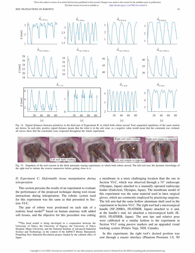
IEEE TRANSACTIONS ON ROBOTICS 16
1
2
3
d[m
m]
1.5
2
2.5
3
1
2
3
1
2
3
18
20
22
24
26
28
d[m
m]
10
12
14
16
18
40
45
50
30
35
40
20 40 60 80
[s]
2
4
6
d[m
m]
20 40 60 80
[s]
0
1
dc1,c2
20 40 60 80
[s]
2
3
4
dl1,pM
20 40 60 80
[s]
3
4
5
dl2,pM
dl1,pNL dl1,pELdl2,pNR
dl2,pER
dπR1,pR2,1dπR1,pR2,2
dπR1,pR2,3dπR1,pR2,4
Fig. 14. Signed distances between primitives in the third part of Experiment B, in which both robots moved. Four sequential repetitions of the same motionare shown. In each plot, positive signed distance means that the robot is in the safe zone; as a negative value would mean that the constraint was violated,all curves show that the constraints were respected throughout the whole experiment.
Left tool starts evading Left tool returns to trajectory
Right tool starts evading Right tool returns to trajectory
Fig. 15. Snapshots of the tool evasion in the third automatic tracing experiment, in which both robots moved. The left tool uses the dynamic knowledge ofthe right tool to initiate the evasive maneuvers before getting close to it.
D. Experiment C: Deformable tissue manipulation during
teleoperation
This section presents the results of an experiment to evaluate
the performance of the proposed technique during tool–tissue
interactions during teleoperation. The robotic system used
for this experiment was the same as that presented in Sec-
tion VI-C.
The pair of robots were positioned on each side of a
realistic head model20 based on human anatomy with added
soft tissues, and the objective for this procedure was cutting
20This head model is being developed in a cooperation between theUniversity of Tokyo, the University of Nagoya, the University of TokyoHospital, Meijo University, and the National Institute of Advanced IndustrialScience and Technology, in the context of the ImPACT Bionic HumanoidsPropelling New Industrial Revolution project funded by the cabined office ofJapan.
a membrane in a more challenging location than the one in
Section VI-C, which was observed through a 70 endoscope
(Olympus, Japan) attached to a manually operated endoscope
holder (EndoArm, Olympus, Japan). The membrane model of
this experiment was the same material used in latex surgical
gloves, which are commonly employed by practicing surgeons.
The left arm had the same hollow aluminum shaft used in the
experiment in Section VI-C. The right tool had a microsurgical
handle (NF-200BA, FEATHER, Japan) attached to it and,
at the handle’s end, we attached a microsurgical knife (K-
6010, FEATHER, Japan). The arm tips and relative pose
were calibrated in a similar fashion to the experiment in
Section VI-C using passive markers and an upgraded visual
tracking system (Polaris Vega, NDI, Canada).
In this experiment, the right tool’s desired position was
sent through a master interface (Phantom Premium 1.0, 3D
This is the author's version of an article that has been published in this journal. Changes were made to this version by the publisher prior to publication.The final version of record is available at http://dx.doi.org/10.1109/TRO.2019.2920078
Copyright (c) 2019 IEEE. Personal use is permitted. For any other purposes, permission must be obtained from the IEEE by emailing [email protected].
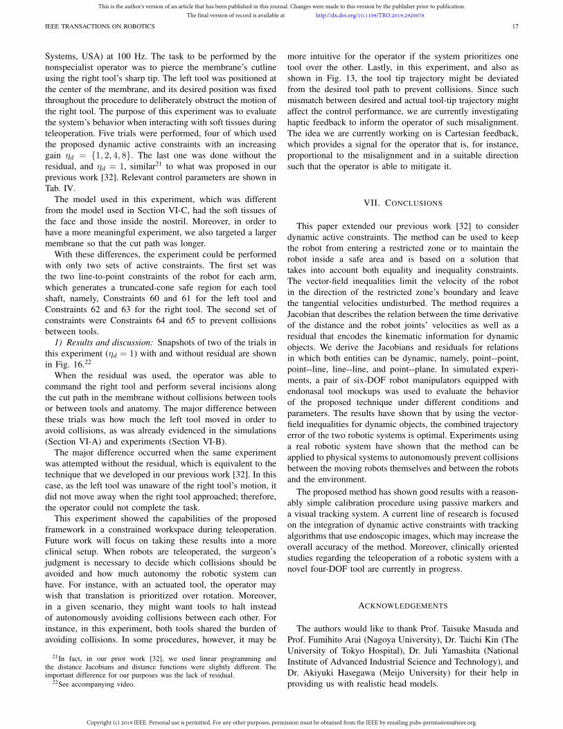
IEEE TRANSACTIONS ON ROBOTICS 17
Systems, USA) at 100 Hz. The task to be performed by the
nonspecialist operator was to pierce the membrane’s cutline
using the right tool’s sharp tip. The left tool was positioned at
the center of the membrane, and its desired position was fixed
throughout the procedure to deliberately obstruct the motion of
the right tool. The purpose of this experiment was to evaluate
the system’s behavior when interacting with soft tissues during
teleoperation. Five trials were performed, four of which used
the proposed dynamic active constraints with an increasing
gain ηd = 1, 2, 4, 8. The last one was done without the
residual, and ηd = 1, similar21 to what was proposed in our
previous work [32]. Relevant control parameters are shown in
Tab. IV.
The model used in this experiment, which was different
from the model used in Section VI-C, had the soft tissues of
the face and those inside the nostril. Moreover, in order to
have a more meaningful experiment, we also targeted a larger
membrane so that the cut path was longer.
With these differences, the experiment could be performed
with only two sets of active constraints. The first set was
the two line-to-point constraints of the robot for each arm,
which generates a truncated-cone safe region for each tool
shaft, namely, Constraints 60 and 61 for the left tool and
Constraints 62 and 63 for the right tool. The second set of
constraints were Constraints 64 and 65 to prevent collisions
between tools.
1) Results and discussion: Snapshots of two of the trials in
this experiment (ηd = 1) with and without residual are shown
in Fig. 16.22
When the residual was used, the operator was able to
command the right tool and perform several incisions along
the cut path in the membrane without collisions between tools
or between tools and anatomy. The major difference between
these trials was how much the left tool moved in order to
avoid collisions, as was already evidenced in the simulations
(Section VI-A) and experiments (Section VI-B).
The major difference occurred when the same experiment
was attempted without the residual, which is equivalent to the
technique that we developed in our previous work [32]. In this
case, as the left tool was unaware of the right tool’s motion, it
did not move away when the right tool approached; therefore,
the operator could not complete the task.
This experiment showed the capabilities of the proposed
framework in a constrained workspace during teleoperation.
Future work will focus on taking these results into a more
clinical setup. When robots are teleoperated, the surgeon’s
judgment is necessary to decide which collisions should be
avoided and how much autonomy the robotic system can
have. For instance, with an actuated tool, the operator may
wish that translation is prioritized over rotation. Moreover,
in a given scenario, they might want tools to halt instead
of autonomously avoiding collisions between each other. For
instance, in this experiment, both tools shared the burden of
avoiding collisions. In some procedures, however, it may be
21In fact, in our prior work [32], we used linear programming andthe distance Jacobians and distance functions were slightly different. Theimportant difference for our purposes was the lack of residual.
22See accompanying video.
more intuitive for the operator if the system prioritizes one
tool over the other. Lastly, in this experiment, and also as
shown in Fig. 13, the tool tip trajectory might be deviated
from the desired tool path to prevent collisions. Since such
mismatch between desired and actual tool-tip trajectory might
affect the control performance, we are currently investigating
haptic feedback to inform the operator of such misalignment.
The idea we are currently working on is Cartesian feedback,
which provides a signal for the operator that is, for instance,
proportional to the misalignment and in a suitable direction
such that the operator is able to mitigate it.
VII. CONCLUSIONS
This paper extended our previous work [32] to consider
dynamic active constraints. The method can be used to keep
the robot from entering a restricted zone or to maintain the
robot inside a safe area and is based on a solution that
takes into account both equality and inequality constraints.
The vector-field inequalities limit the velocity of the robot
in the direction of the restricted zone’s boundary and leave
the tangential velocities undisturbed. The method requires a
Jacobian that describes the relation between the time derivative
of the distance and the robot joints’ velocities as well as a
residual that encodes the kinematic information for dynamic
objects. We derive the Jacobians and residuals for relations
in which both entities can be dynamic, namely, point--point,
point--line, line--line, and point--plane. In simulated experi-
ments, a pair of six-DOF robot manipulators equipped with
endonasal tool mockups was used to evaluate the behavior
of the proposed technique under different conditions and
parameters. The results have shown that by using the vector-
field inequalities for dynamic objects, the combined trajectory
error of the two robotic systems is optimal. Experiments using
a real robotic system have shown that the method can be
applied to physical systems to autonomously prevent collisions
between the moving robots themselves and between the robots
and the environment.
The proposed method has shown good results with a reason-
ably simple calibration procedure using passive markers and
a visual tracking system. A current line of research is focused
on the integration of dynamic active constraints with tracking
algorithms that use endoscopic images, which may increase the
overall accuracy of the method. Moreover, clinically oriented
studies regarding the teleoperation of a robotic system with a
novel four-DOF tool are currently in progress.
ACKNOWLEDGEMENTS
The authors would like to thank Prof. Taisuke Masuda and
Prof. Fumihito Arai (Nagoya University), Dr. Taichi Kin (The
University of Tokyo Hospital), Dr. Juli Yamashita (National
Institute of Advanced Industrial Science and Technology), and
Dr. Akiyuki Hasegawa (Meijo University) for their help in
providing us with realistic head models.
This is the author's version of an article that has been published in this journal. Changes were made to this version by the publisher prior to publication.The final version of record is available at http://dx.doi.org/10.1109/TRO.2019.2920078
Copyright (c) 2019 IEEE. Personal use is permitted. For any other purposes, permission must be obtained from the IEEE by emailing [email protected].
IEEE TRANSACTIONS ON ROBOTICS 18
00:06W
ithout
resi
dual
Wit
hre
sidual
The left tool deviates to avoid collision
The left tool stays in place
00:00 00:45 00:54 Task impossible
00:00 00:42 00:57 01:40 Task completed
Fig. 16. Results of two of the trials described in Section VI-D. The first row shows the trial with no residual and ηd = 1 (equivalent to [32]), in whichthe left tool is unaware of the right tool’s motion and therefore it does not move away, therefore it was impossible to perform the cutting task. The secondrow shows one of the trials in which the residual is used and ηd = 1. By adding the residual, the centralized optimization problem makes the left toolautomatically move away to reduce the overall trajectory tracking error, making it possible to perform the cutting task.
REFERENCES
[1] H. Ueda, R. Suzuki, A. Nakazawa, Y. Kurose, M. M. Marinho, N. Shono,H. Nakatomi, N. Saito, E. Watanabe, A. Morita, K. Harada, N. Sugita,and M. Mitsuishi, “Toward autonomous collision avoidance for roboticneurosurgery in deep and narrow spaces in the brain,” Procedia CIRP,vol. 65, no. Supplement C, pp. 110 – 114, 2017. 3rd CIRP Conferenceon BioManufacturing.
[2] M. Marinho, A. Nakazawa, J. Nakanishi, T. Ueyama, Y. Hasegawa,J. Arata, M. Mitsuishi, and K. Harada, “Conceptual design of a ver-satile robot for minimally invasive transnasal microsurgery,” in Micro-
NanoMechatronics and Human Science (MHS), 2016 International Sym-
posium on, pp. 1–3, IEEE, 2016.
[3] A. Morita, S. Sora, M. Mitsuishi, S. Warisawa, K. Suruman, D. Asai,J. Arata, S. Baba, H. Takahashi, R. Mochizuki, et al., “Microsurgicalrobotic system for the deep surgical field: development of a prototypeand feasibility studies in animal and cadaveric models,” Journal of
neurosurgery, vol. 103, no. 2, pp. 320–327, 2005.
[4] Y. Ida, N. Sugita, T. Ueta, Y. Tamaki, K. Tanimoto, and M. Mitsuishi,“Microsurgical robotic system for vitreoretinal surgery,” International
journal of computer assisted radiology and surgery, vol. 7, no. 1, pp. 27–34, 2012.
[5] M. Mitsuishi, A. Morita, N. Sugita, S. Sora, R. Mochizuki, K. Tanimoto,Y. M. Baek, H. Takahashi, and K. Harada, “Master–slave robotic plat-form and its feasibility study for micro-neurosurgery,” The International
Journal of Medical Robotics and Computer Assisted Surgery, vol. 9,no. 2, pp. 180–189, 2013.
[6] A. Nakazawa, K. Nanri, K. Harada, S. Tanaka, H. Nukariya, Y. Kurose,N. Shono, H. Nakatomi, A. Morita, E. Watanabe, et al., “Feedbackmethods for collision avoidance using virtual fixtures for robotic neu-rosurgery in deep and narrow spaces,” in Biomedical Robotics and
Biomechatronics (BioRob), 2016 6th IEEE International Conference on,pp. 247–252, IEEE, 2016.
[7] L. Wu, S. Song, K. Wu, C. M. Lim, and H. Ren, “Development of acompact continuum tubular robotic system for nasopharyngeal biopsy,”Medical & Biological Engineering & Computing, vol. 55, pp. 403–417,may 2016.
[8] H. Yu, L. Wu, K. Wu, and H. Ren, “Development of a multi-channelconcentric tube robotic system with active vision for transnasal nasopha-ryngeal carcinoma procedures,” IEEE Robotics and Automation Letters,vol. 1, pp. 1172–1178, jul 2016.
[9] R. Taylor, P. Jensen, L. Whitcomb, A. Barnes, R. Kumar, D. Stoianovici,P. Gupta, Z. Wang, E. Dejuan, and L. Kavoussi, “A steady-hand roboticsystem for microsurgical augmentation,” The International Journal of
Robotics Research, vol. 18, no. 12, pp. 1201–1210, 1999.
[10] J. G. Petersen, S. A. Bowyer, and F. R. y Baena, “Mass and frictionoptimization for natural motion in hands-on robotic surgery,” IEEE
Transactions on Robotics, vol. 32, no. 1, pp. 201–213, 2016.
[11] B. Siciliano, L. Sciavicco, L. Villani, and G. Oriolo, Robotics: Mod-
elling, Planning and Control. Advanced Textbooks in Control and SignalProcessing, London: Springer-Verlag London, 2009.
[12] A. Kapoor, M. Li, and R. H. Taylor, “Constrained control for surgicalassistant robots.,” in Robotics and Automation (ICRA), 2006 IEEE
International Conference on, pp. 231–236, 2006.
[13] M. Li, M. Ishii, and R. H. Taylor, “Spatial motion constraints usingvirtual fixtures generated by anatomy,” IEEE Transactions on Robotics,vol. 23, no. 1, pp. 4–19, 2007.
[14] S. A. Bowyer, B. L. Davies, and F. R. y Baena, “Active con-straints/virtual fixtures: A survey,” IEEE Transactions on Robotics,vol. 30, no. 1, pp. 138–157, 2014.
[15] Z. Chen, A. Malpani, P. Chalasani, A. Deguet, S. S. Vedula,P. Kazanzides, and R. H. Taylor, “Virtual fixture assistance for needlepassing and knot tying,” in Intelligent Robots and Systems (IROS), 2016
IEEE/RSJ International Conference on, pp. 2343–2350, IEEE, 2016.
[16] M.-A. Vitrani, C. Poquet, and G. Morel, “Applying virtual fixturesto the distal end of a minimally invasive surgery instrument,” IEEE
Transactions on Robotics, vol. 33, no. 1, pp. 114–123, 2017.
[17] T. L. Gibo, L. N. Verner, D. D. Yuh, and A. M. Okamura, “Designconsiderations and human-machine performance of moving virtual fix-tures,” in Robotics and Automation, 2009. ICRA’09. IEEE International
Conference on, pp. 671–676, IEEE, 2009.
[18] K.-W. Kwok, G. P. Mylonas, L. W. Sun, M. Lerotic, J. Clark, T. Athana-siou, A. Darzi, and G.-Z. Yang, “Dynamic active constraints for hyper-redundant flexible robots,” in International Conference on Medical
Image Computing and Computer-Assisted Intervention, pp. 410–417,Springer, 2009.
[19] N. V. Navkar, Z. Deng, D. J. Shah, K. E. Bekris, and N. V. Tsekos,“Visual and force-feedback guidance for robot-assisted interventionsin the beating heart with real-time mri,” in Robotics and Automation
(ICRA), 2012 IEEE International Conference on, pp. 689–694, IEEE,2012.
[20] F. Rydén and H. J. Chizeck, “Forbidden-region virtual fixtures fromstreaming point clouds: Remotely touching and protecting a beatingheart,” in Intelligent Robots and Systems (IROS), 2012 IEEE/RSJ In-
ternational Conference on, pp. 3308–3313, IEEE, 2012.
[21] J. Ren, R. V. Patel, K. A. McIsaac, G. Guiraudon, and T. M. Peters,“Dynamic 3-d virtual fixtures for minimally invasive beating heartprocedures,” IEEE transactions on medical imaging, vol. 27, no. 8,pp. 1061–1070, 2008.
[22] K.-W. Kwok, K. H. Tsoi, V. Vitiello, J. Clark, G. C. Chow, W. Luk,and G.-Z. Yang, “Dimensionality reduction in controlling articulatedsnake robot for endoscopy under dynamic active constraints,” IEEE
Transactions on Robotics, vol. 29, no. 1, pp. 15–31, 2013.
[23] K.-W. Kwok, V. Vitiello, and G.-Z. Yang, “Control of articulated snakerobot under dynamic active constraints,” Medical Image Computing and
Computer-Assisted Intervention–MICCAI 2010, pp. 229–236, 2010.
[24] B. C. Becker, R. A. MacLachlan, L. A. Lobes, G. D. Hager, and C. N.Riviere, “Vision-based control of a handheld surgical micromanipulatorwith virtual fixtures,” IEEE Transactions on Robotics, vol. 29, no. 3,pp. 674–683, 2013.
[25] J. Burgner, D. C. Rucker, H. B. Gilbert, P. J. Swaney, P. T. Russell, K. D.
This is the author's version of an article that has been published in this journal. Changes were made to this version by the publisher prior to publication.The final version of record is available at http://dx.doi.org/10.1109/TRO.2019.2920078
Copyright (c) 2019 IEEE. Personal use is permitted. For any other purposes, permission must be obtained from the IEEE by emailing [email protected].
IEEE TRANSACTIONS ON ROBOTICS 19
Weaver, and R. J. Webster, “A telerobotic system for transnasal surgery,”IEEE/ASME Transactions on Mechatronics, vol. 19, pp. 996–1006, jun2014.
[26] K. Wu, G. Zhu, L. Wu, W. Gao, S. Song, C. M. Lim, and H. Ren,“Safety-enhanced model-free visual servoing for continuum tubularrobots through singularity avoidance in confined environments,” IEEE
Access, pp. 1–1, 2019.
[27] J. Funda, R. H. Taylor, B. Eldridge, S. Gomory, and K. G. Gruben,“Constrained cartesian motion control for teleoperated surgical robots,”IEEE Transactions on Robotics and Automation, vol. 12, no. 3, pp. 453–465, 1996.
[28] T. Xia, C. Baird, G. Jallo, K. Hayes, N. Nakajima, N. Hata, andP. Kazanzides, “An integrated system for planning, navigation androbotic assistance for skull base surgery,” The International Journal of
Medical Robotics and Computer Assisted Surgery, vol. 4, no. 4, pp. 321–330, 2008.
[29] R. Prada and S. Payandeh, “On study of design and implementation ofvirtual fixtures,” Virtual reality, vol. 13, no. 2, pp. 117–129, 2009.
[30] B. Faverjon and P. Tournassoud, “A local based approach for pathplanning of manipulators with a high number of degrees of freedom,”in Robotics and Automation. Proceedings. 1987 IEEE International
Conference on, vol. 4, pp. 1152–1159, IEEE, 1987.
[31] O. Kanoun, F. Lamiraux, and P.-B. Wieber, “Kinematic control ofredundant manipulators: Generalizing the task-priority framework toinequality task,” IEEE Transactions on Robotics, vol. 27, no. 4, pp. 785–792, 2011.
[32] M. M. Marinho, B. V. Adorno, K. Harada, and M. Mitsuishi, “Activeconstraints using vector field inequalities for surgical robots,” in 2018
IEEE International Conference on Robotics and Automation (ICRA),pp. 5364–5371, May 2018.
[33] B. V. Adorno, Two-arm Manipulation: From Manipulators to Enhanced
Human-Robot Collaboration [Contribution à la manipulation à deux
bras : des manipulateurs à la collaboration homme-robot]. PhDDissertation, Université Montpellier 2, 2011.
[34] A. T. Yang, Application of quaternion algebra and dual numbers to the
analysis of spatial mechanisms. PhD thesis, Columbia University., 1963.
[35] A. Perez and J. M. McCarthy, “Dual Quaternion Synthesis of Con-strained Robotic Systems,” Journal of Mechanical Design, vol. 126,no. 3, pp. 425–435, 2004.
[36] J. J. Quiroz-Omaña and B. V. Adorno, “Whole-Body Kinematic Controlof Nonholonomic Mobile Manipulators Using Linear Programming,”Journal of Intelligent & Robotic Systems, vol. 91, pp. 263–278, 10 2017.
[37] B. V. Adorno, “Robot kinematic modeling and control based on dualquaternion algebra — Part I: Fundamentals,” 2017.
[38] J. M. Selig, Geometric fundamentals of robotics. Springer-Verlag NewYork Inc., 2nd ed., 2005.
[39] B. V. Adorno, P. Fraisse, and S. Druon, “Dual position control strategiesusing the cooperative dual task-space framework,” in Intelligent Robots
and Systems (IROS), 2010 IEEE/RSJ International Conference on,pp. 3955–3960, IEEE, 2010.
[40] S. Boyd and L. Vandenberghe, Convex optimization. Cambridge univer-sity press, 2004.
[41] A. Escande, N. Mansard, and P.-B. Wieber, “Hierarchical quadraticprogramming: Fast online humanoid-robot motion generation,” The
International Journal of Robotics Research, vol. 33, pp. 1006–1028,may 2014.
[42] M. Marinho, L. Figueredo, and B. V. Adorno, “A dual quaternionlinear-quadratic optimal controller for trajectory tracking,” in Intelligent
Robots and Systems (IROS), 2015 IEEE/RSJ International Conference
on, pp. 4047–4052, IEEE, 2015.
[43] T. Brox, B. Rosenhahn, J. Gall, and D. Cremers, “Combined regionand motion-based 3d tracking of rigid and articulated objects,” IEEE
Transactions on Pattern Analysis and Machine Intelligence, vol. 32,no. 3, pp. 402–415, 2010.
[44] E. Rohmer, S. P. Singh, and M. Freese, “V-rep: A versatile and scalablerobot simulation framework,” in Intelligent Robots and Systems (IROS),
2013 IEEE/RSJ International Conference on, pp. 1321–1326, IEEE,2013.
[45] Z. Zador and K. Gnanalingham, “Endoscopic transnasal approach tothe pituitary – operative technique and nuances,” British Journal of
Neurosurgery, vol. 27, pp. 718–726, may 2013.
[46] A. Huaulmé, K. Harada, G. Forestier, M. Mitsuishi, and P. Jannin,“Sequential surgical signatures in micro-suturing task,” Int. J. Computer
Assisted Radiology and Surgery, vol. 13, no. 9, pp. 1419–1428, 2018.
[47] R. G. Chittawadigi and S. K. Saha, “An analytical method to detectcollision between cylinders using dual number algebra,” in Intelligent
Robots and Systems (IROS), 2013 IEEE/RSJ International Conference
on, pp. 5353–5358, IEEE, 2013.[48] S. Agarwal, R. A. Srivatsan, and S. Bandyopadhyay, “Analytical de-
termination of the proximity of two right-circular cylinders in space,”Journal of Mechanisms and Robotics, vol. 8, no. 4, p. 041010, 2016.
Murilo Marques Marinho (GS’13–M’18) receivedthe bachelor’s degree in mechatronics engineeringand the master’s degree in electronic systems and au-tomation engineering from the University of Brasilia,Brasilia, Brazil, in 2012 and 2014, respectively. Hereceived the Ph.D. degree in mechanical engineeringfrom the University of Tokyo, Tokyo, Japan, in2018. In 2018, he was a Visiting Researcher withthe Johns Hopkins University. He is an AssistantProfessor with the University of Tokyo from 2019.His research interests include robotics applied to
medicine, robot control theory, and image processing.
Bruno Vilhena Adorno (GS’09–M’12–SM’17) re-ceived the BS degree (2005) in Mechatronics En-gineering and the MS degree (2008) in ElectricalEngineering, both from the University of Brasilia,Brasilia, Brazil, and the PhD degree (2011) fromUniversity of Montpellier, Montpellier, France. Heis currently a Tenured Assistant Professor with theDepartment of Electrical Engineering at the FederalUniversity of Minas Gerais, Belo Horizonte, Brazil.His current research interests include both practicaland theoretical aspects related to robot kinematics,
dynamics, and control with applications to mobile manipulators, humanoidsand cooperative manipulation systems.
Kanako Harada (M’07) received the B.E. andM.E. degrees from The University of Tokyo, Tokyo,Japan, and the Ph.D. degree in engineering fromWaseda University, Tokyo, in 1999, 2001, and2007, respectively. After working with Hitachi,Ltd.,Waseda University, the National Center forChild Health and Development, the Scuola SuperioreSant’Anna, the University of Tokyo, and the JapanScience and Technology Agency (JST), she wasappointed as a Associate Professor at The Universityof Tokyo in 2015. Her research interests include
medical and surgical robotics.
Mamoru Mitsuishi (M’93) received the master’sand D.E. degrees in mechanical engineering fromthe University of Tokyo, Tokyo, Japan, in 1983and 1986, respectively. In 1986, he was a Lecturerwith the University of Tokyo, where he was alsoan Associate Professor in 1989 and a Professorsince 1999. From 1987 to 1988, he was a VisitingResearcher with the Fraunhofer Institute for Produc-tion Technique and Automation, Stuttgart, Germany.His research interests include computer integratedsurgical systems and manufacturing systems.
This is the author's version of an article that has been published in this journal. Changes were made to this version by the publisher prior to publication.The final version of record is available at http://dx.doi.org/10.1109/TRO.2019.2920078
Copyright (c) 2019 IEEE. Personal use is permitted. For any other purposes, permission must be obtained from the IEEE by emailing [email protected].