Dunne, Timothy, Lucia Foster, John Haltiwanger and Kenneth R ...

National Opinion Research Center

Wage and Productivity Dispersion in United States Manufacturing: The Role of ComputerInvestmentAuthor(s): Timothy Dunne, Lucia Foster, John Haltiwanger, Kenneth R. TroskeSource: Journal of Labor Economics, Vol. 22, No. 2 (Apr., 2004), pp. 397-429Published by: The University of Chicago Press on behalf of the Society of Labor Economists andthe National Opinion Research Center.Stable URL: http://www.jstor.org/stable/3653629Accessed: 06/10/2010 17:18

Your use of the JSTOR archive indicates your acceptance of JSTOR's Terms and Conditions of Use, available athttp://www.jstor.org/page/info/about/policies/terms.jsp. JSTOR's Terms and Conditions of Use provides, in part, that unlessyou have obtained prior permission, you may not download an entire issue of a journal or multiple copies of articles, and youmay use content in the JSTOR archive only for your personal, non-commercial use.

Please contact the publisher regarding any further use of this work. Publisher contact information may be obtained athttp://www.jstor.org/action/showPublisher?publisherCode=ucpress.

Each copy of any part of a JSTOR transmission must contain the same copyright notice that appears on the screen or printedpage of such transmission.

JSTOR is a not-for-profit service that helps scholars, researchers, and students discover, use, and build upon a wide range ofcontent in a trusted digital archive. We use information technology and tools to increase productivity and facilitate new formsof scholarship. For more information about JSTOR, please contact [email protected].

The University of Chicago Press and National Opinion Research Center are collaborating with JSTOR todigitize, preserve and extend access to Journal of Labor Economics.

http://www.jstor.org

http://www.jstor.org/action/showPublisher?publisherCode=ucpress

http://www.jstor.org/action/showPublisher?publisherCode=norc

http://www.jstor.org/stable/3653629?origin=JSTOR-pdf

http://www.jstor.org/page/info/about/policies/terms.jsp

http://www.jstor.org/action/showPublisher?publisherCode=ucpress

Wage and Productivity Dispersion in United States Manufacturing: The Role

of Computer Investment

Timothy Dunne, University of oklahoma

Lucia Foster, U.s. Bureau of the Census

John Haltiwanger, University of Maryland

Kenneth R. Troske, University of Missouri-Columbia

Using establishment-level data, we shed light on the sources of the changes in the structure of production, wages, and employment that have occurred over recent decades. Our findings are: (1) the between- plant component of wage dispersion is an important and growing part of total wage dispersion; (2) much of the between-plant increase in wage dispersion is within industries; (3) the between-plant measures of wage and productivity dispersion have increased substantially over recent decades; and (4) a significant fraction of the rising

We would like to thank Robert Topel, Andrew Hildreth, and seminar partic- ipants at Carnegie-Mellon, the Federal Reserve Bank of Kansas City, Harvard, Institute for the Study of Labor (IZA), Massachusetts Institute of Technology, and University of California, Los Angeles, for helpful comments. All opinions, findings, and conclusions expressed herein are ours and do not in any way reflect the views of the U.S. Census Bureau. The data used in this article were collected under the provisions of Title 13 U.S. Code and are only available at the Center for Economic Studies, U.S. Census Bureau. To obtain access to these data, contact the Center for Economic Studies, U.S. Census Bureau, RM 211/WPII, Washing- ton, DC 20233. Contact the corresponding author, Kenneth R. Troske, at [email protected].

[Journal of Labor Economics, 2004, vol. 22, no. 2] ? 2004 by The University of Chicago. All rights reserved. 0734-306X/2004/2202-0006$10.00

397

398 Dunne et al.

dispersion in wages and productivity is accounted for by changes in the distribution of computer investment across plants.

I. Introduction

It is a well-documented empirical finding that from the mid-1970s through the early 1990s the United States experienced a significant increase in wage inequality. Acemoglu (2002) reports that the difference in wages earned by a worker in the ninetieth percentile of the wage distribution compared to a worker in the tenth percentile increased by 38% in the United States from 1971 to 1995. One hypothesis offered to explain this rise in wage inequality is skill-biased technical change. That is, the introduction of advanced technologies and, in particular, the widespread diffusion of computers has led to a rising demand for skilled workers, which, in turn, has led to a rise in the wages of skilled workers relative to unskilled workers.

This article attempts to shed new light on the skill-biased technical change hypothesis by exploiting establishment-level data to investigate changes in the dispersion of wages and productivity across establishments and the role of technical change in accounting for the observed changes in dispersion. The focus on between-establishment changes in wages and productivity is a novel feature of our analysis. This focus is motivated by recent theoretical papers hypothesizing that technical change occurs through differential technology adoption by plants in the same industry.1 If plants do adopt technologies at different rates, and new technology is skill biased, this should lead to cross-plant changes in the dispersion of wages and productivity. If rising wage dispersion is indeed a between- plant phenomenon, this in turn suggests that we can use differences in technology use across plants to examine the role of skill-biased technical change. Accordingly, we perform three exercises in this article. First, we examine whether the increase in wage dispersion is primarily a between- plant phenomenon. Second, we examine whether plant-level changes in wages and productivity appear to be linked. Finally, we ask whether between-plant changes in wage and productivity dispersion can be ex- plained by differential technology adoption across producers.

Our article attempts to connect several strands of the literature studying wages, productivity, and computers. Many recent studies have sought to understand either the relationship between computer use and wages (e.g., Krueger 1993; Doms, Dunne, and Troske 1997; Autor, Katz, and Krueger 1998) or, alternatively, computer use and productivity (e.g., Oliner and

SKatz and Autor (1999) and Acemoglu (2002) provide comprehensive reviews of the recent theoretical and empirical literature analyzing the link between wages, wage inequality, and technology.

The Role of Computer Investment 399

Sichel 1994; Greenan and Mairesse 1996; Siegel 1997; Bresnahan, Bryn- jolfsson, and Hitt 2002). One of our main objectives is to investigate these relationships simultaneously.

As a starting point, our analysis builds upon the separate literature that exploits plant-level data and finds that the overall increase in wage inequality between workers is closely tied to an increase in the dispersion of wages between establishments (e.g., Davis and Haltiwanger 1991). This research documents that much of the increase in the between-plant dispersion of wages is a within-industry phenomenon so that the full ex- ploration of these differences requires plant-level data as opposed to industry-level data. Moreover, research on plant-level productivity shows that there is also tremendous within-industry variation in productivity across plants and that much of the increase in aggregate (industry-level) productivity is associated with the reallocation of resources from less productive to more productive plants within the same industry (Baily, Hulten, and Campbell 1992; Olley and Pakes 1996; Foster, Haltiwanger, and Krizan 2001). Unlike with wages, however, there has been little analysis of changes in the dispersion of productivity over time and little analysis of the role of advanced technology and computers in accounting for the observed differences in productivity across plants.2

The article proceeds as follows. In Section II we briefly discuss the relevant theoretical literature that helps motivate the subsequent empirical analysis. In Section III we decompose the total dispersion in hourly wages into within and between components over the 1975-92 period. We find that virtually the entire increase in overall dispersion in hourly wages for U.S. manufacturing workers from 1975 to 1992 is accounted for by the between-plant components. This result is quite important as it is at the core of the hypotheses we are investigating.

In Section IV we examine the links between productivity and wages. At the aggregate level, we find that the between-plant dispersion of both wages and productivity increased over the 1975-92 period. At the plant level, we find that wages and productivity are strongly positively correlated in both levels and changes. In Section V we investigate the source of the changes in the dispersion of wages and productivity by examining the role of computer investment in accounting for the across-plant differences in wages and labor productivity. We find that a significant percentage of the observed changes in the dispersion of wages and (to a lesser extent) productivity is accounted for by changes in the distributions of computer investment as well as changes in the wage and productivity

2 One exception is the work of Dwyer (1995), who examines the relationship between productivity and wage dispersion for the textile industry. He finds that plants in the textile industry with higher-than-average total factor productivity residuals also pay higher-than-average wages.

400 Dunne et al.

differentials associated with computer investment. Section VI summarizes the main findings and provides a discussion of alternative interpretations of our findings.

II. Review of Theoretical Literature

Our empirical analysis explores the role of between-plant versus within- plant changes in accounting for changes in wage dispersion, and how the differential use of technology across plants accounts for between-plant changes in wage and productivity dispersion. There are a variety of mech- anisms through which technical change is hypothesized to affect the distribution of wages and the structure of the workforce. Acemoglu (2002) provides a comprehensive review of both the theoretical and empirical literature. Two specific lines of research help frame our empirical analysis. The first line considers the role of skill-biased technological revolutions. This literature emphasizes the role that the introduction of new technologies plays in changing the relative demand for workers. Papers in this line of research include Greenwood, Hercowitz, and Krusell (1997), Greenwood and Yorukoglu (1997), and Caselli (1999). The second line of research examines the relationship between technological change and organizational change. Here, the premise is that technological change can lead to changes in the organizational structure of firms that affect the distribution of wages and the composition of firm workforces. Acemoglu (1999) and Kremer and Maskin (2000) construct models where technological change can lead to increases in plant-level segregation of workers by skill.3 In the remainder of this section, we use the papers by Caselli (1999) and Kremer and Maskin (2000) to illustrate these ideas and to help develop empirical predictions regarding technological change and the distributions of plant-level wages, skill, and productivity.

Caselli (1999) models the effect of a technical revolution on the dispersion of wages and productivity. In the Caselli model there is a distribution of worker types and types of machines. Operating a given type of machine requires a specific type of skill. The cost of learning a given skill varies across workers with the costs being lower for more skilled workers. A technology is a matching of workers of type i who have the appropriate set of skills to operate machines of type i. An important feature of this model for our purposes is that workers are completely segregated by skill across plants. A technological revolution occurs with the development of a new type of machine.4 A revolution is skill biased

3 Papers by Bresnahan (1999) and Autor, Levy, and Murnane (2002) also argue that recent technological changes lead to changes in the organization of production.

4 Examples of new types of machines mentioned by Caselli are the assembly line, the steam engine, and information technologies or computers.


if the skills required to operate the new machine are more costly for workers to acquire than existing skills. Therefore, when a skill-biased revolution occurs, high-skilled workers will be the first to use the new machines since it is less costly for these workers to acquire the new skills. Low-skilled workers will continue to use the old machines because technologies have diminishing marginal returns and all types of machines must have the same rate of return in equilibrium. This model has three implications that are relevant for our analysis. First, since more skilled workers are using more and better capital relative to less skilled workers, a skill- biased technical revolution leads to an increase in the dispersion of wages across plants.5 Second, since skilled workers are using more and better machines, a skill-biased technical revolution also leads to an increase in the dispersion of labor productivity across plants. Third, the relative increases in wages and productivity should be associated with the adoption of new technology.

Kremer and Maskin (2000) also provide a theoretical structure for our empirical analysis. Their model can account for the simultaneous existence of increased wage inequality and increased segregation across plants of workers of different skill. These forces are set in motion by changes in the skill distribution, which can be due to a skill-biased technical change, but need not be. The main features of their model are imperfect substi- tution among workers of different skills, complementary tasks within a plant, differences in worker skill effects that vary by task, and an exog- enous distribution of worker skills.6 Intuitively, there are two competing forces at work in determining the equilibrium matching patterns at plants. The asymmetry of tasks in the production function favors cross-matching (less segregation), but the complementarity between tasks favors self- matching (more segregation). Unequally skilled workers will be cross- matched up to the point at which the differences in skills are so great that the second effect overwhelms the first and the plant moves to self- matching. When the overall distribution of skills is sufficiently com- pressed, high- and low-skilled workers will be matched together in the same plant. When the distribution of skills is sufficiently diffuse, there will be complete segregation of workers by skill across plants. With a diffuse skill distribution, an increase in the mean skill-level exacerbates wage inequality across plants.

The Kremer-Maskin model has three implications relevant for our analysis. First, increases in the cross-worker dispersion of skill result in in-

5 Whether this increase in relative wages persists depends on a number of factors outlined in Caselli (1999).

6 In the Kremer-Maskin model there is a set number of tasks that must be performed in order to produce one unit of output, and overall productivity is a multiplicative function of each task. Tasks are complementary in the sense that the output from any task affects the marginal productivity of all other tasks.

402 Dunne et al.

creased segregation of workers by skill across plants. Second, if the overall distribution of skill is sufficiently dispersed, an increase in the mean level of worker skill will lead to an increase in the dispersion of wages across skill levels and plants. Third, if the overall distribution of skill is sufficiently dispersed, an increase in the mean level of skill leads to an increase in the cross-plant dispersion of productivity.

The hypothesis that skill-biased technical change can affect the demand for skilled workers and the structure of wages and productivity is consistent with a large class of models. We focus on the models of Caselli (1999) and Kremer and Maskin (2000) because both speculate that technical adoption and changes in the distribution of wages and productivity will be a between-plant, as opposed to a within-plant, phenomenon. The general point is that, in principle, the increased demand for skilled workers driven by skill-biased technical change could have occurred within the typical or representative establishment. Accordingly, the rising wage dispersion and/or changes in the skill of workers could be seen within the representative establishment by increases in the within-establishment dispersion of wages. In contrast, the between-plant hypothesis predicts that skill-biased technical change will be associated with greater dispersion in wages and technology across establishments with much smaller changes occurring within the representative establishment. This greater dispersion in wages and productivity results from increased skill segregation, which in turn is the result of differential rates of technical adoption across plants. Our use of establishment-level data provides a basis for evaluating the relevance and validity of these predictions that focus on between-establishment changes.

III. Between-Plant and Within-Plant Components of Wage Dispersion

In this section, we combine data from household and establishment surveys to decompose the variance of hourly wages in manufacturing into between-plant and within-plant components. The decomposition methodology is from Davis and Haltiwanger (1991, 1996); however, we extend their analysis in three ways. First, we use a more comprehensive data set that permits inclusion of auxiliary establishments (e.g., central adminis- trative offices, research facilities, and warehouses). Second, we use a more general version of the decomposition that permits decomposing the wage gap between production and nonproduction workers into within- and between-plant components. Third, we use a more recent time period, 1977-92, while Davis and Haltiwanger considered the period 1973-86. Similar to Davis and Haltiwanger, we decompose the hourly wage variance into production and nonproduction worker components because we feel that workers in these two groups have very different skills. The decom-


position expresses the total variance of hourly wages as the hours- weighted sum of the variances of production and nonproduction workers' wages along with a term reflecting the contribution of differences in the mean wages across production and nonproduction workers. Thus, the variance of hourly wages in the manufacturing sector is decomposed as

V = oVP

+ (1 - a)Vn + (1 - a)(WP - Wn)2,(1)

where ca denotes production workers' share of hours worked, VP denotes the variance of production worker hourly wages, Vn denotes the variance of nonproduction worker hourly wages, WP is the hours-weighted mean of the production worker wage, and Wn is the hours-weighted mean of the nonproduction worker wage. For each worker type, the variance can be further decomposed as

Vi = Vip + V5P for j = p,n, (2)

where Vip represents the between-plant component and V1, the within- plant component for worker type j.

We use household data from the March Current Population Survey (CPS) and establishment data from the Longitudinal Research Database (LRD) to estimate the components of the decomposition for the manufacturing sector.7 From the individual-level wage observations in the CPS files, we calculate cx,V, VP, Vh, WP, We for all workers employed in manufacturing in each of the years under consideration (1975-92). We also generate the production and nonproduction variances at the two-digit SIC industry level. From the plant-level observations in the LRD, we calculate the between-plant component for each worker type for each of the corresponding years at the two-digit level. For each worker type, we generate the within-plant component in equation (2) by taking the difference between the total variance calculated from the CPS and the between-plant variance calculated from the LRD at the two-digit level.s Appropriately aggregating the between-plant and within-plant components across industries yields the decomposition at the total manufacturing level.

As part of the decomposition, we decompose the overall between-plant component for each worker type

(Vr,) into a between-plant, within-in-

dustry component (VApi)

and a between-industry component (VA). De- composing wage variation into a between-plant, within-industry com-

7 The data appendix provides a detailed discussion of the issues that arise when combining information from household and establishment surveys. These measurement difficulties suggest that the results in Sec. III must be interpreted with appropriate caution. However, these measurement difficulties should primarily affect levels rather than time series changes.

8 Summary statistics for the CPS and LRD wage data are presented in table Al of the data appendix.

404 Dunne et al.

ponent and a between-industry component allows us to distinguish between changes that are due to the movement of workers between industries and changes that are due to shifts between plants in the same industry. Presumably, the former movement is related to product demand shifts, while the latter movement is more closely tied to productivity changes among producers of similar products. In this analysis, industries are defined at the two-digit level.

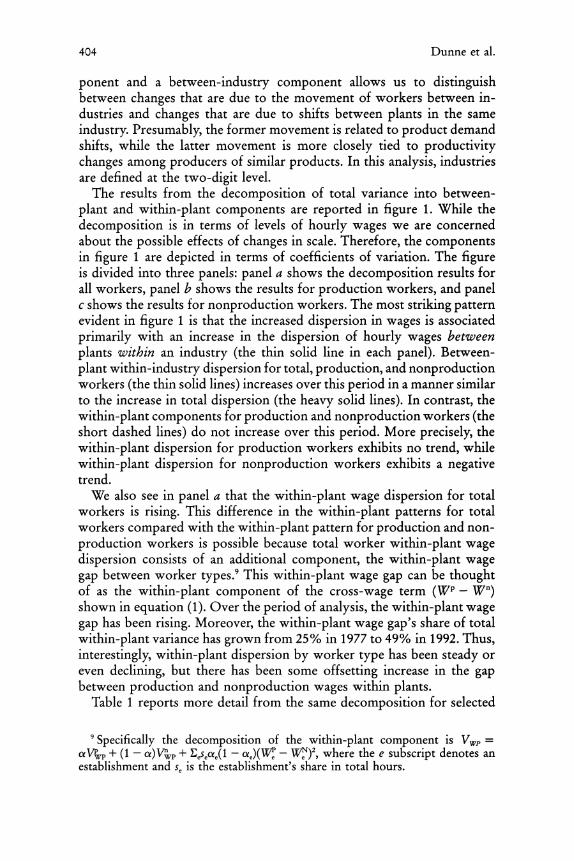
The results from the decomposition of total variance into between- plant and within-plant components are reported in figure 1. While the decomposition is in terms of levels of hourly wages we are concerned about the possible effects of changes in scale. Therefore, the components in figure 1 are depicted in terms of coefficients of variation. The figure is divided into three panels: panel a shows the decomposition results for all workers, panel b shows the results for production workers, and panel c shows the results for nonproduction workers. The most striking pattern evident in figure 1 is that the increased dispersion in wages is associated primarily with an increase in the dispersion of hourly wages between plants within an industry (the thin solid line in each panel). Between- plant within-industry dispersion for total, production, and nonproduction workers (the thin solid lines) increases over this period in a manner similar to the increase in total dispersion (the heavy solid lines). In contrast, the within-plant components for production and nonproduction workers (the short dashed lines) do not increase over this period. More precisely, the within-plant dispersion for production workers exhibits no trend, while within-plant dispersion for nonproduction workers exhibits a negative trend.

We also see in panel a that the within-plant wage dispersion for total workers is rising. This difference in the within-plant patterns for total workers compared with the within-plant pattern for production and nonproduction workers is possible because total worker within-plant wage dispersion consists of an additional component, the within-plant wage gap between worker types.9 This within-plant wage gap can be thought of as the within-plant component of the cross-wage term (WP - Wn) shown in equation (1). Over the period of analysis, the within-plant wage gap has been rising. Moreover, the within-plant wage gap's share of total within-plant variance has grown from 25% in 1977 to 49% in 1992. Thus, interestingly, within-plant dispersion by worker type has been steady or even declining, but there has been some offsetting increase in the gap between production and nonproduction wages within plants.

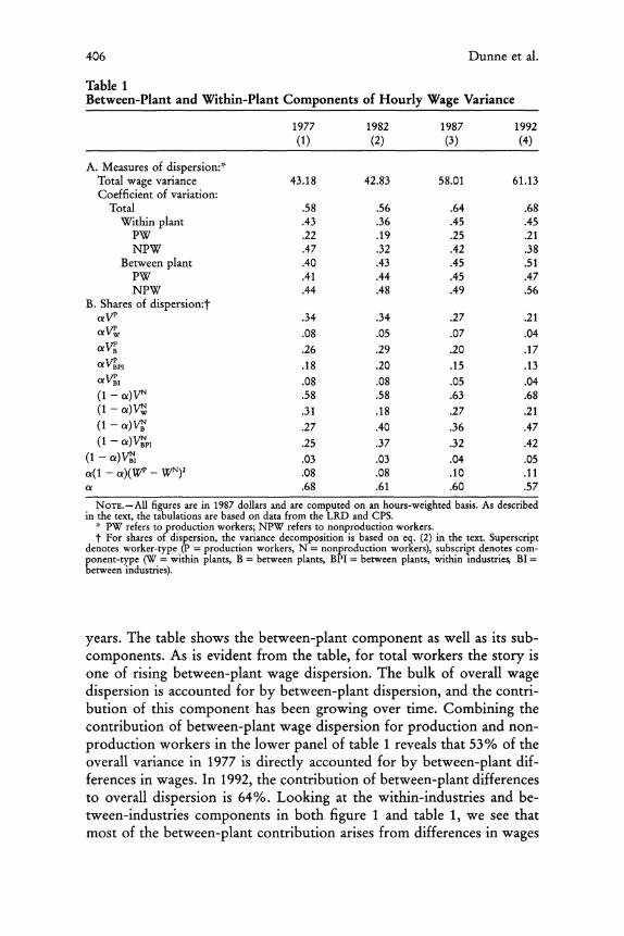
Table 1 reports more detail from the same decomposition for selected

SSpecifically the decomposition of the within-plant component is Vw =

aVp + (1 - a) Vypn

+ LeSeQe(1 - ae)(W - WN)2, where the e subscript denotes an

establishment and s~e is the establishment's share in total hours.

a = 0.7

0.6

S0.5

f30.4 - + .8 0.3

Cc 0.2- -- - -- -----

S0.1 75 76 77 78 79 80 81 82 83 84 85 86 87 88 89 90 91 92

Year

b o 0.7

. 0.6

• 0.5 o 0.4

., 0.3- S0.2- _.---

-U

O0.1

75 76 77 78 79 80 81 82 83 84 85 86 87 88 89 90 91 92

Year

C

= 0.7

S0.6

; 0.5- ,, 0.4

.• 0.3

•02-- u 0 .1 I , i , , , I , i t , , ..

75 76 77 78 79 80 81 82 83 84 85 86 87 88 89 90 91 92

Year __ Total - Between Plant,

Within Industry

. Within Plant - - Between Industry

FIG. 1.-Coefficient of variation for hourly wages. a, Total workers; b, production workers; c, nonproduction workers.

406 Dunne et al.

Table 1 Between-Plant and Within-Plant Components of Hourly Wage Variance

1977 1982 1987 1992 (1) (2) (3) (4)

A. Measures of dispersion:*' Total wage variance 43.18 42.83 58.01 61.13 Coefficient of variation:

Total .58 .56 .64 .68 Within plant .43 .36 .45 .45

PW .22 .19 .25 .21 NPW .47 .32 .42 .38

Between plant .40 .43 .45 .51 PW .41 .44 .45 .47 NPW .44 .48 .49 .56

B. Shares of dispersion:t aVP .34 .34 .27 .21

oV• .08 .05 .07 .04

o!V• .26 .29 .20 .17 aVC PI .18 .20 .15 .13 a V1 .08 .08 .05 .04 (1 - a)VN .58 .58 .63 .68 (1 - a)V" .31 .18 .27 .21 (1 - a)VN .27 .40 .36 .47 (1 - a))V~1 .25 .37 .32 .42

(1 - e) V" .03 .03 .04 .05 Ca(1 - a)(Wp - WN)2 .08 .08 .10 .11 a .68 .61 .60 .57

NOTE.--AI1 figures are in 1987 dollars and are computed on an hours-weighted basis. As described in the text, the tabulations are based on data from the LRD and CPS.

* PW refers to production workers; NPW refers to nonproduction workers. t For shares of dispersion, the variance decomposition is based on eq. (2) in the text. Superscript

denotes worker-type (P = production workers, N = nonproduction workers), subscript denotes component-type (W = within plants, B = between plants, BPI = between plants, within industries, BI = between industries).

years. The table shows the between-plant component as well as its sub- components. As is evident from the table, for total workers the story is one of rising between-plant wage dispersion. The bulk of overall wage dispersion is accounted for by between-plant dispersion, and the contribution of this component has been growing over time. Combining the contribution of between-plant wage dispersion for production and nonproduction workers in the lower panel of table 1 reveals that 53% of the overall variance in 1977 is directly accounted for by between-plant differences in wages. In 1992, the contribution of between-plant differences to overall dispersion is 64%. Looking at the within-industries and between-industries components in both figure 1 and table 1, we see that most of the between-plant contribution arises from differences in wages


between plants within the same industry.10 The result that much of the increase is due to an increase in the between-plant dispersion within industries indicates that explanations that rely on shifts between industries (e.g., simple product demand shifts across industries) cannot account for the rising dispersion.

There is greater wage dispersion among nonproduction workers than among production workers. This fact combined with an increased nonproduction worker labor share over this time period has yielded an increasing share of overall dispersion being accounted for by differences in wages among nonproduction workers. Another contributing factor to overall increases in wage dispersion is a widening gap between production and nonproduction worker wages. The gap between production and nonproduction worker wages accounts for 8% of overall dispersion in 1977 and 11% of overall dispersion in 1992.

While it is not the focus of our analysis, there is also a distinct cyclical pattern evident in table 1 in the respective components of the decomposition, especially for the within-plant components. For production and especially nonproduction workers, the within-plant dispersion of wages falls between 1977 and 1982 and then rebounds somewhat by 1987. The cyclical decrease in the within-plant components is sufficiently large that the overall variance of wages falls slightly between 1977 and 1982. The overall variance increases strongly from 1982 to 1987, reflecting the com- bination of the cyclical rebound of the within-plant components and the secular increase in the between-plant component. The overall variance continues to increase from 1987 and 1992, reflecting the secular increase in the between-plant component."

We feel that the primary source of the observed movements between 1977 and 1982 and 1982 and 1987 in the within-plant component is cyclical fluctuation in the labor market (e.g., low wage workers being laid off at plants during a recession and the movement of workers into and out of the labor market over the business cycle) and has relatively little to do with the adoption of new technologies on the part of the plant. One piece

'o In earlier versions of the article, we also document that the increase in the between-plant wage dispersion is a within-industry phenomenon at the four-digit industry level. The results in this section only consider the two-digit industry level, since this is the level of aggregation at which the LRD and CPS statistics can be readily matched. See Dunne et al. (2000).

" Note that the between-plant component rises throughout this period. The different cyclical patterns imply that the fraction of the overall variance accounted for by the between-plant component actually peaks in 1982. However, as noted in the discussion, this is due to cyclical factors that actually cause the overall variance to fall between 1977 and 1982. These cyclical factors are not the focus of our analysis. The secular trend is for the between-plant component to rise over the period and the fraction accounted for by the between-plant component to rise.

408 Dunne et al.

of the evidence supportive of this view is that the between-plant component of the variance of wages rises monotonically over the entire period. As we argued in Section II, recent models predict that if the changing technology is skill biased then its adoption will be associated with rising between-plant dispersion, and the steady increase in between-plant dispersion is consistent with such long run changes in technology. Therefore, we focus most of our attention on the overall increase in dispersion that occurs between 1977 and 1992, which we believe is the result of secular changes such as the introduction of new technology.

In summary, we find that the between-plant components of dispersion are an important fraction of overall wage dispersion and account for much of the increase in overall dispersion in the 1975-92 period. These results parallel and extend similar findings in Davis and Haltiwanger (1991, 1996) and in Kremer and Maskin (2000). Moreover, we believe the evidence in this section makes a strong case that accounting for the sources of the increase in overall wage dispersion necessitates accounting for the sources of the increase in between-plant wage dispersion.

IV. Linking Productivity and Wages

In this section, we provide a basic description of the relationship between wages and productivity at the sector and plant level. Panel a of figure 2 presents two different wage dispersion series. Using data from the March Current Population Survey (CPS), the heavy line in panel a depicts the 90-10 differential of log hourly wages for 1975-92.2 As is now well known, there has been a sustained increase in the dispersion of wages among workers over this period of time. Somewhat less well known is that the increase in dispersion among all workers is mimicked by an increase in dispersion among manufacturing workers. Again, using the CPS, the thin line in the panel a shows that the pattern for manufacturing workers closely tracks that for all workers.

Panel b of figure 2 depicts the between-plant hours-weighted 90-10 differential of log productivity across U.S. manufacturing plants (the heavy line) and the between-plant 90-10 differential of plant-level log average hourly wages (the thin line). We measure productivity as the log of output per hour worked, defined as the log of the total value of ship- ments from the plant, measured in constant 1987 dollars, divided by total

12 The 90-10 differential is measured as the difference between the hourly log wage for the worker at the ninetieth percentile of the hourly log wage distribution for a given year and the hourly log wage of the worker at the tenth percentile of this distribution. In this and subsequent analysis using 90-10 differentials, the respective distributions are the total hours weighted distributions across plants or workers. Details of measurement of wages and productivity from the CPS and LRD are discussed in the data appendix.

a

1 .6 - -

1 .5

-~1.4

1.3 -

o 1.2

1.1

74 76 78 80 82 84 86 88 90 92 94

Year

..... -AII ---- .

M anuf.

b 2

1.9

1.8

1.7 "a .,-1.6-

1.3

1.2 -

1.1

74 76 78 80 82 84 86 88 90 92 94

Year

- --- P ro d u c tivity ......- ..

W age

FIG. 2.-Dispersion in log worker wages and productivity. a, Wage dispersion; b, between- plant productivity and wage dispersion.

410 Dunne et al.

plant hours.13 The output data are deflated using the four-digit industry price deflators found in the Bartelsman and Gray (1996) productivity data set. As is the case for wages, productivity dispersion also exhibits a sustained increase over this time period.

Comparing the movements in the two dispersions series suggests that it may be possible to identify common factors underlying the secular increases in wage and productivity dispersion. Both dispersion series de- cline slightly between 1981 and 1982 and between 1984 and 1986, while rising steadily between 1986 and 1992. However, there are some notable differences in the timing of the secular changes. While most of the increase in between-plant wage dispersion occurs between 1979 and 1987, productivity dispersion increases steadily only after the early 1980s recession, with most of the increase occurring between 1986 and 1992. The differing cyclical fluctuations of dispersion of wages and productivity may reflect a variety of factors such as cyclical variation in capacity utilization and/ or factors relevant for the cyclicality of wages. If new information technology (IT) is at the core of the shifts in these distributions, then the timing of the shifts in the distribution may not be synchronized. Stiroh (2002) argues that the effect of IT on productivity becomes stronger over time because the technology obtained a critical mass in the mid- to late 1990s. Bresnahan et al. (2002, p. 346) argue that the complementary factors of IT investment, organization change, and human capital will have "different adjustment costs and adjustment speeds." Differential learning and adjustment costs imply that changes in the actual distribution of the workforce may precede changes in the distribution of productivity. While these high-frequency timing issues are clearly of interest, we have chosen to focus on long-run changes in this article because we feel it is important to understand the causes of the secular changes in these variables, and because we feel these are the changes that we are best able to examine given our data. As such, in what follows when we analyze the factors driving wages and productivity dispersion, we will primarily focus on the long-run change from 1977 to 1992.

13 We measure labor productivity using gross output rather than value-added because gross output is measured more accurately than value-added and value- added at the establishment level is negative (as it can be) in a nontrivial number of cases, making it difficult to use the log of plant-level productivity to compute a dispersion measure. We believe that the 90-10 differentials in log productivity and log wages are more robust measures of dispersion than raw productivity and wages. Note, however, that many studies using the LRD have found a very high correlation between labor productivity measured using gross output or value added (see, e.g., Baily, Bartelsman, and Haltiwanger 1996, 2001). As in the previous section, we estimate the number of hours for nonproduction workers based on the CPS average annual hours worked per nonproduction worker for each two- digit industry and apply these two-digit aggregate average hours worked for a nonproduction worker to the plant-level nonproduction worker variable.


A comparison of the aggregate data series suggest that there may be a link between changes in wage dispersion and changes in productivity dispersion in the manufacturing sector. However, for the analysis we are undertaking, it is also important to establish that there is a link between productivity and wages at the plant level. The simple cross-sectional correlation between plant-level wages and labor productivity averages .55, indicating that plants that have higher wages also tend to have higher levels of labor productivity. This correlation is almost constant over time, varying between .52 and .57 for all years between 1975 and 1992, and is statistically significant at the .005 level in all years. We also construct the correlation between plant-level changes in wages and plant-level changes in productivity by using data on 12,904 plants that appear in our data in the four census years: 1977, 1982, 1987, and 1992.'4 The correlations are .35 for the 1977-82 period, .36 for the 1982-87 period, and .39 for the 1987-92 period, and all are statistically significant at the .005 level.

We interpret the simple correlations as demonstrating that there exists a positive cross-plant relationship in the level of wages and productivity and a positive cross-plant relationship in the changes in wages and productivity. We interpret the aggregate time series presented in figure 2 as evidence that both cross-plant changes in wage and productivity dispersion are moving in a similar manner over the long run. In the remainder of the article, we examine more closely the changes in cross-plant wage and productivity distributions and relate these changes to the differential adoption patterns of new computing technology across producers.

V. Computer Investment and the Dispersion of Wages and Productivity

In this section we investigate the relationship between changes in technology and changes in wage and productivity dispersion. Clearly, one important technological change that occurred over the last 3 decades has been the diffusion of computing technologies throughout the economy. This widespread diffusion is observed in manufacturing as well. Figure 3 depicts the frequency of computer investment in plants over the period. In 1977, only 10% of reporting plants indicated purchases of computing equipment as part of their overall investment. By 1992, this number had risen to over 60%.5 In the remainder of this section, we will explore the link between the changes in the distribution of computer investment ob-

14 Census years are the only years for which we can measure changes for all of the surviving plants in our data.

15 Every 5 years, the Annual Survey of Manufactures (ASM) asks manufacturing plants about their investment expenditures on computers and transportation equipment. In each year, roughly 60% of plants respond to this part of the survey form. However, these responding plants account for almost 90% of machinery investment in a given year.

412 Dunne et al.

0.7

0.6

0.5

0.4

0

0

0.3

0.2

0.1

1977 1982 1987 1992

Year

FIG. 3.-Proportion of plants investing in computers

served in figure 3 and changes in the dispersion of wages and productivity reported earlier in the article.

Our approach will follow Juhn, Murphy, and Pierce (1993), and, in particular, Davis and Haltiwanger (1991, 1996), who utilize the Juhn et al. full distribution accounting methodology in a similar setting. The analysis starts with the specification of a basic regression model of the following form:

Yit = Xitt + cit, (3)

where our plant-level variable of interest, y,, is wages, productivity, or workforce structure for plant i in period t, X;, is a matrix of observable plant characteristics, f, is a parameter vector, and I, is the residual of the regression.

The estimated parameters from this model do not have a direct structural interpretation, rather they are measures of the covariance structure in the data between measures of outcomes and plant characteristics. For example, the coefficients may reflect unobserved technology effects that


are correlated with computer investment. In our setting, it is explicitly hypothesized that such unobserved technology effects may be correlated with observables like computer intensity. Moreover, the theories we are investigating suggest that the nature of these unobserved technology effects may have changed over time (e.g., skill-biased technical change that is embodied in observable indicators of technology like computer intensity) so that the covariance between measures of outcomes, like productivity, and measures of technology, such as computer investment, may have changed over time.

Our approach is to decompose the change in the dispersion of the dependent variable

(yi,) into three components based on the regression

model-changes in the distribution of observable plant characteristics (changes in the X's), changes in the differentials associated with the effect of the observables on the dependent variable (changes in the P's), and changes in the distribution of the unobservables (changes in the

/'s). That

is, consider the following version of equation (3):

Yi, = X

it

+ Xi,(t,

- f) + i;,,

(4)

where 3 is the average effect of the observables on the dependent variable over the whole period. Using equation (4) as a starting point, we decompose the change in the 90-10 differential of y, between 1977 and 1992 into three components. First, using the actual distribution of the left-hand side variable in equation (4) for 1977 and 1992, we compute the change in the 90-10 differential of y;, from 1977 to 1992. Next, we compute the predicted change using the first term on the right-hand side of equation (4) to generate the 90-10 differential in 1977 and the 90-10 differential in 1992 to compute the predicted change from the X's alone. Comparing the predicted to the actual change in the 90-10 differential yields a measure of the change in the dispersion of y, attributable to the change in the distribution of observable characteristics (the X's). Next we compute the predicted change using both the first and second terms of equation (4). This latter predicted change captures the impact of both changes in the distribution of the X's and changes in the j's. To obtain the marginal contribution of just the f's, we compare this change with the change in the overall distribution attributable to the change in the distribution of the X's.'6 The marginal contribution of changes in the distribution of the residuals is then just the total change in the 90-10 differential of the actual distribution minus the change due to changes in both the X's and the f's.

16 We should note that it is possible to get different results depending on the order of the decomposition as well as which year serves as the base year. We deliberately chose to put observable quantities first to give them the greatest opportunity to account for the changes in dispersion.

414 Dunne et al.

A. The Data

The data used to examine the between-plant changes in the dispersion of productivity, wages, and workforce composition come from the same source as the plant-level wage data employed in the prior section. Our analysis focuses on explaining the changes in dispersion in five plant-level variables: the log of average plant hourly wages, the log of average plant production worker hourly wages, the log of average plant nonproduction worker hourly wages, the nonproduction labor share of employment, and the log of output per hour. The wage and productivity variables are measured in the same fashion as in the preceding section. The nonproduction labor share variable is our attempt to capture changes in the composition of the workforce in manufacturing establishments. It is measured as the total wages paid to nonproduction workers divided by the total wages paid to all workers in the plant. In papers such as Berman, Bound, and Griliches (1994), Dunne, Haltiwanger, and Troske (1997), Autor et al. (1998), Caselli (1999), and Kremer and Maskin (2000), this variable is interpreted as representing a measure of workforce skill.17

The observable plant characteristics contained in the X matrix in equation (4) include four-digit SIC industry controls, nine census region dummies, nine size class dummies, a multiunit dummy variable, capital intensity, and computer investment as a fraction of total investment. In what follows, we permit the coefficients on each of the plant measures (i.e., size dummies, multiunit dummy, capital intensity, and computer investment) to vary by two-digit industry.

The computer investment variable is constructed as the ratio of computer investment in a plant to total investment in a plant. While we would prefer to have a measure of the stock of the computing equipment at each point in time, this information is simply unavailable.18 Berman et al. (1994) and Autor et al. (1998) use this same variable as their measure of computer use (though at the industry level).19 While our measure does not capture

17 Both Berman et al. (1994) and Dunne et al. (1997) discuss at considerable length the strengths and weaknesses of using nonproduction labor share as a measure of skill. It is well documented that nonproduction workers are generally more educated than production workers as a group. However, it is also the case that the nonproduction worker group includes both workers that would be considered more skilled than the typical production workers (engineers, managers, programmers) and also a set of workers that may be less skilled (janitors, guards).

18 We also experimented with using a zero-one dummy variable indicating whether or not a plant was currently investing in computing equipment in place of the ratio variable. The regression and Juhn et al. decomposition results that follow are, in general, qualitatively similar across these definitions.

19 See Troske (1996) for a detailed discussion of the computer investment question on the ASM. The use of the computer investment variable restricts our analysis to census years (the only years the computer investment question is asked) and reduces the sample size because of the lower response rate to this question.


Table 2 Descriptive Statistics of LRD Data Set

1977 1992

90-10 90-10 Mean Differential Mean Differential

(1) (2) (3) (4)

Log hourly wage 2.46 .90 2.42 1.02 Log production worker hourly

wage 2.36 .98 2.29 1.07 Log nonproduction worker

hourly wage 2.69 .90 2.67 1.03 Nonproduction labor share .27 .46 .32 .58 Log output per hour 3.82 1.71 4.12 1.88 Computer investment

to total investment ratio .04 .08 .14 .42

NOTE.--The restricted sample includes only plants that report detailed investment data.

the stock of computing capital at a plant, we believe it is a reasonable (though imperfectly measured) indicator of plants that have advanced technology on site.

Table 2 presents some basic descriptive statistics for each of the variables for the years 1977 and 1992. The statistics are hours-weighted means and 90-10 differentials. The data used in the analysis include all plants that report detailed investment data and represent about 60% of all plants in the ASM in each year (between 30,000 and 35,000 plants each year). The basic statistics show that the between-plant dispersion in wage, productivity, and nonproduction labor share has increased over the 15-year period. These patterns for productivity and wages were noted earlier in the article. The bottom row reports the summary statistics for the computer investment variable. Both the mean and 90-10 differential in the computer investment variable have increased over time. The sharp rise in the mean of computer investment as a fraction of total investment represents two forces at work. First, the percentage of plants that report positive investment expenditures on computing equipment rises sharply over the period. Second, the mean computer investment as a fraction of total investment for plants with positive spending on computer investment increased over the period as well.

B. Regression Results

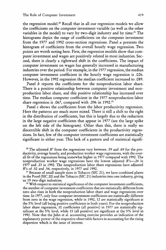
Before proceeding to the Juhn et al. full distribution accounting exercises, we present summary information regarding the effect of computer investment on our main variables of interest. Figure 4 has three panels and in each panel is a plot of the computer investment coefficients from

P '

0\

a 7

6

5

0 "1977"

E l "1l992" z

-0.2 -0.175 -0.15 -0.125 -0.1 -0.075 -0.05 -0.025 0 0.025 0.05 0.075 0.1 0.125 0.15 0.175 0.2

Coefficient Values

FIG. 4.-Computer investment coefficients. a, Overall hourly wage coefficients.

-P r V

b 6

5

4

0 "1977" ii

:3

=• "1992" z

2

0

.. .11•, I .[LII -0.2 -0.175 -0.15 -0.125 -0.1 -0.075 -0.05 -0.025 0 0.025 0.05 0.075 0.1 0.125 0.15 0.175 0.2

Coefficient Values

FIG. 4.-b, Nonproduction labor share coefficients

C 8

7

6

?-0 "1977" 4

I "1992" E

Z3

2

0 -0.2 -0.18 -0.15 -0.13 -0.1 -0.08 -0.05 -0.03 0 0.025 0.05 0.075 0.1 0.125 0.15 0.175 0.2

Coefficient Values

FIG. 4.-c, Labor productivity coefficients


the regression model.20 Recall that in all our regression models we allow the coefficients on the computer investment variable (as well as the other variables in the model) to vary by two-digit industry and by time.21 The histograms depict the range of coefficients on the computer investment from the 1977 and 1992 cross-section regressions. Panel a presents the histogram of coefficients from the overall hourly wage regression. Two points are worth noting here. First, the regression models show that computer investment and wages are positively related in most industries. Sec- ond, there is clearly a rightward shift in the coefficients. The impact of computer investment on wages has generally increased in manufacturing industries over the period. For example, in the 1977 regression, the median computer investment coefficient in the hourly wage regression is .026. However, in the 1992 regression the median coefficient increased to .089.

Panel b reports the coefficients for the nonproduction labor share. There is a positive relationship between computer investment and nonproduction labor share, and this positive relationship has increased over time. The median computer coefficient in the 1977 nonproduction labor share regression is .067, compared with .096 in 1992.22

Panel c shows the coefficients from the labor productivity regression. Here the patterns are much more mixed. There is still a shift to the right in the distribution of coefficients, but this is largely due to the reduction in the large negative coefficients that appear in 1977 (see the large spike on the left side of the histogram). Other than this, there is really no discernible shift in the computer coefficients in the productivity regressions. In fact, few of the computer investment coefficients are statistically significant in either year. This lack of a pattern and of statistical signifi-

20 The adjusted R2 from the regressions vary between .59 and .69 for the productivity, average hourly, and production worker wage regressions, with the overall fit of the regressions being somewhat higher in 1977 compared with 1992. The nonproduction worker wage regressions have the lowest adjusted R2s-.24 in 1977 and .23 in 1992. The nonproduction labor share regressions have adjusted R2s of .52 and .54, respectively, in 1977 and 1992.

21 Because of small sample sizes in Tobacco (SIC 21), we have combined plants in the Food (SIC 20) and the Tobacco (SIC 21) industries into one industry, giving us 19 two-digit industries.

22 With respect to statistical significance of the computer investment coefficients, the number of computer investment coefficients that are statistically different from zero also rises in both the nonproduction labor share and wage regressions over time. In 1977, only four computer investment coefficients are statistically different from zero in the wage regression, while in 1992, 12 are statistically significant at the 5% level (all being positive coefficients in both years). For the nonproduction labor share regression, 10 coefficients (all positive) in 1977 are statistically significant at the 5% level, while 15 (all positive) are significant at the 5% level in 1992. Note that the Juhn et al. accounting exercise provides an indication of the explanatory power of the respective observable factors in accounting for the rising dispersion which is the issue of interest.

420 Dunne et al.

cance in the coefficients is consistent with the finding in other studies that look at the relationship between computers and productivity using data from the late 1970s and 1980s. For example, the paper by Berndt and Morrison (1995), which uses capital stock data on office and computing equipment as their measure of advanced technology, also reports widely varying correlations between computers and productivity at the two-digit level.

A more recent study by Brynjolfsson and Hitt (2003) finds a relatively strong positive relationship between the stock computer equipment and productivity.23 One particular strength of the Brynjolfsson and Hitt study is in their measure of computer capital. Brynjolfsson and Hitt have constructed data on computer stocks based on detailed information on the composition of machines used by a firm. This is clearly superior to the measure that we have available. However, by doing so, they focus on a much smaller set of very large firms. In contrast, our data contains both small and large establishments and in each year includes more than 30,000 manufacturing plants. Our data differ from their data in other ways as well, and these differences also account for the different findings. First, our data include a large number of producers that are making no investments in computer equipment in a year. This is especially true in 1977, when investment in computing equipment is relatively rare. Second, our data cover a key 15-year period and allow us to observe the diffusion in computer equipment. Given our focus on the changing nature of the between-plant distribution of computers, it is important that we capture the diffusion process in our analysis. Finally, Brynjolfsson and Hitt's data come from the period 1987-94, whereas our data come from the late 1970s and early 1990s. Studies that use data from the mid- to late 1990s tend to find a much stronger relationship between productivity and computer capital. For example, a recent industry-level study by Stiroh (2002) shows that the impact of information technology on labor productivity is strongly positive in the mid- to late 1990s but is weak in the 1970s up through the early 1990s.

It is important to note that while we do not observe strong and consistent relationships between computers and productivity across all our industries, we do find systematic and consistent relationships between computers and our variables measuring worker skill. Plants investing in computing equipment pay higher average hourly wages and employ a greater share of nonproduction labor. Hence, we believe that our com-

23 Brynjolfsson and Yang (1996) provide an overview of the IT productivity literature. In general, they report that earlier studies based on data from the 1970s and 1980s find a much weaker relationship between IT and productivity than studies using data from the 1990s.


Table 3 Decomposing Changes in the Dispersion of Wages, Skill, and Productivity

Nonproduc- Hourly Production Nonproduc- tion Labor Labor Pro- Wage Wages tion Wages Share ductivity

(1) (2) (3) (4) (5)

Total 1977-92 change .118 .093 .128 .111 .161 Marginal contribution of

computer investment: Observables .033 .020 .025 .041 .033 Betas .012 .013 .014 .003 -.010 Unobservables .073 .060 .090 .068 .137

puter measure is picking up systematic differences in plant operations that are associated with technological change.24

Of course, caution must be used in translating these changes in average industry coefficients into the implied changes in wage and productivity dispersion, since ultimately we need to consider the interaction between the changes in the coefficients for every industry and the changes in the dispersion in computer intensities in each industry. Indeed, it is via the Juhn et al. decomposition exercises that we consider this interaction, since the Juhn et al. methodology itself provides the appropriate weighting and aggregation of the changes in characteristics and the changes in differentials associated with these characteristics.

C. Full Distribution Accounting Results

Utilizing the information from the regressions, we examine changes in the dispersion of the between-plant wages, labor productivity, and workforce structure using the Juhn et al. decomposition analysis discussed above. We focus our attention here on the role of computer investments; however, we have examined the role of capital and plant size in earlier versions of the article.25 The first row of table 3 reports the overall changes in the 90-10 differentials for our five variables that occurred between 1977 and 1992. For all five variables there was an increase in the 90-10 differ-

24 These results are similar to results found in Wolff (2002), who uses industry data from the 1960s through the 1980s and finds that computerization is relatively uncorrelated with productivity but is positively correlated with occupational re- structuring in industries.

25 See Dunne et al. (2000) for the Juhn et al. decomposition analysis of changes in dispersion for the three subperiods 1977-82, 1982-87, and 1987-92 and for detailed analysis of the role of capital intensity and size. The marginal contributions of both of the latter variables are positive and significant in a manner that is consistent with the skill-biased technical change hypothesis. For example, the marginal contribution of changes in the distribution of capital intensity plus the changes in the 3's for capital intensity help account for rising wage and productivity dispersion.

422 Dunne et al.

entials. The next three rows provide an accounting of the marginal contribution of computer investment for our five variables. We construct the marginal contribution of computer investment in the following manner. We set all other right-hand side variables at their sample means and use the pooled coefficients for all other variables and then consider the marginal contribution of the computer investment variable to the changes in dispersion. That is, we consider the contribution of the change in the distribution of computer investment and its differential in isolation, having controlled for the influence of all of the other variables. Note that this

implies that the contribution of unobservables reported when we conduct one of the marginal exercises includes the influence of time variation in the distribution of the other observable variables and their differentials

(3's). The results for hourly wages, production wages, and nonproduction

wages all show that rising wage dispersion is accounted for by increases in the dispersion of computer investment. Both the changes in the dispersion in the computer investment variable and the influence of the change in the 3's help account for the changes in the observed wage dispersion. These patterns hold true when we disaggregate wages by production and nonproduction labor (table 3, cols. 2 and 3). Column 4 reports the results for the nonproduction labor share (our measure of workforce skill), and it is again the case that both the shift in the 3's and the increasing dispersion of computer investment help account for the increase in dispersion in workforce structure, though most of the contribution comes from the observables category.

The results on labor productivity are more mixed (table 3, col. 5). The rise in dispersion in computer investment (holding the 3's fixed) certainly helps explain the rise in between-plant productivity dispersion. However, the 3's work in the opposite direction; the shift in the 3's on the computer variables that occurred between 1977 and 1992 actually leads to a lower dispersion in labor productivity. On balance, however, the net effect (the effect of both the observables and the 3's) of computer investment on productivity dispersion is to increase dispersion.

These results document the fact that differences in technology use across plants are closely related to rising wage and productivity dispersion in manufacturing. It is important to emphasize that the finding of an important role for computer investment is based on an analysis that controls for many other factors as well. Among these other factors are size and capital intensity. The covariation in the direct measures of technology, wages, and productivity across plants is consistent with the earlier theoretical discussion that identifies rising wage and productivity dispersion as potentially due to differential adoption of advanced technology across plants.


VI. Summary and Interpretation of Findings

This article has documented and analyzed changes in the dispersion in wages and productivity for the manufacturing sector. Our main findings are that (1) the between-plant component of wage dispersion is an important and growing part of total wage dispersion, (2) much of the between-plant increase in wage dispersion is within industries, (3) the between-plant measures of wage and productivity dispersion have increased substantially over the last few decades, and (4) rising dispersion in wages and (to a lesser extent) productivity is accounted for by changes in the distribution of computer investment across plants.

The results are broadly consistent with models like that of Kremer and Maskin (2000) regarding skill segregation across plants and that of Caselli (1999) regarding the role of differential technology adoption across plants in an environment with skill segregation and skill-biased technical change. These models predict rising between-plant wage and productivity dispersion, which is consistent with our findings. Moreover, the Kremer and Maskin model predicts an increase in segregation by worker skill across plants, which is also consistent with our findings. In addition, the Caselli model predicts that the rising wage and productivity dispersion across plants will be associated with differences in technology adoption across plants in response to a skill-biased technological revolution. Our findings support this latter prediction in the sense that we find that a substantial fraction of the rising wage and productivity dispersion is accounted for by rising wage and productivity differentials across plants with different computer intensities.

While the results are broadly consistent with the hypothesis that differential technology adoption across plants accounts for the rising dispersion in wages and productivity, there are other possible explanations that are also consistent with these results. For example, consider a shift in demand between products classified in the same four-digit industry (due to, say, changing trade patterns), where these products are produced in different plants in the industry, and where these plants differ syste- matically in the skill of workers. A shift toward the products produced in plants employing high-skilled workers and away from products produced in plants employing low-skilled workers could yield rising wage dispersion across plants in the same industry and rising measured productivity dispersion. The latter effect could occur because four-digit price deflators would not capture the relative price change within the industry, resulting in systematic productivity mismeasurement across plants in the same industry. However, even under this scenario one would still have to account for the observed pattern of rising wage and productivity dispersion resulting from changes in computer investment across plants. And while there might be a systematic relationship between product mix, skill

424 Dunne et al.

mix, and technology used at the plant, such a systematic relationship would begin to make this scenario resemble a broadly defined notion of skill-biased technical change.

One could likewise argue that changes in institutions could yield a pattern of within-industry, between-plant increases in wage and productivity dispersion. Consider the possible impact of deunionization. De- unionization may have produced less wage compression and a relaxation of work rule constraints that resulted in an increase in wage and productivity dispersion across plants. However, one would again need to account for the fact that this rising wage and productivity dispersion is associated with changes in the distribution of computer investment across plants.

To conclude, we have documented that the rising overall wage dispersion in the U.S. economy is associated with rising wage and productivity dispersion across plants within the same narrowly defined industries. Moreover, a substantial fraction of this rising wage and productivity dispersion is accounted for by changes in the distribution of computer investment. Such findings are consistent with models of increased segregation by skill across plants and rising wage and productivity dispersion from skill-biased technical change that involves differential adoption of new technologies across plants. It may be that there are other models/ hypotheses consistent with these findings, but they will have to account for both the dominant role of between-plant effects and the important role of computer investment across plants.

Data Appendix

Combining Household and Establishment Survey Data: Measurements Issues

Several measurement error issues arise in combining information from household and establishment surveys. Since Davis and Haltiwanger (1991) provide an extensive discussion of these issues in this context, we review only the most salient issues here. First, unlike Davis and Haltiwanger (1991), we incorporate auxiliary establishments into our analysis using data from the Standard Statistical Establishment List (SSEL), which includes the universe of all establishments in each year. Therefore, our establishment-level data contain wage information for all manufacturing workers.

Second, like Davis and Haltiwanger (1991, 1996), we must confront the difficulties associated with the fact that we have hours data only for production workers. We impute hours per worker for nonproduction workers in our augmented LRD as follows. Using the CPS, we calculate the ratio of hours per worker for production and nonproduction workers at the two-digit level. Using this ratio, and the measured hours per worker for production workers at the plant level in the LRD, we impute the hours per worker for nonproduction workers in a plant by requiring that


Table Al Mean and Standard Deviation of Worker Wages (1987 Dollars)

LRD with Auxiliary Establish- Augmented

CPS LRD ment LRD*

Mean SD Mean SD Mean SD Mean SD Year (1) (2) (3) (4) (5) (6) (7) (8)

A. All workers: 1977 11.24 6.57 11.76 4.11 12.14 4.61 11.96 4.49 1982 11.62 6.54 12.07 4.45 12.59 5.21 12.30 5.01 1987 11.88 7.62 12.45 4.69 12.95 5.55 12.67 5.38 1992 11.49 7.82 11.87 4.81 12.55 5.96 12.31 5.86

B. Nonproduction workers:

1977 13.97 8.93 15.04 5.98 15.58 6.35 14.96 6.10 1982 13.96 8.00 14.95 6.28 15.78 6.97 14.95 6.65 1987 14.78 9.55 16.01 6.63 16.69 7.53 15.97 7.23 1992 14.47 9.82 15.25 7.16 16.35 8.30 15.80 8.17

C. Production workers:

1977 9.98 4.62 10.68 4.06 10.68 4.06 10.68 4.06 1982 10.13 4.88 10.83 4.48 10.83 4.48 10.83 4.48 1987 9.92 5.11 10.67 4.45 10.67 4.45 10.67 4.45 1992 9.23 4.76 9.91 4.33 9.91 4.33 9.91 4.33 * For Augmented LRD, the LRD wages for nonproduction workers have been adjusted so that the

ratio of hourly wages for production and nonproduction workers in the LRD is the same as that in the CPS at the two-digit industry level.

the ratios be the same in the CPS and the LRD.26 Since this is at best a crude procedure, we further adjust the LRD means and variances of hourly wages for nonproduction workers so that the ratio of the LRD to CPS mean of hourly wages for nonproduction workers equals the corresponding ratio for production workers.27 We carry out this latter adjustment at the two-digit industry level (i.e., we do not require this ratio to hold at the plant level).

While this methodology for combining household- and establishment- level data may be imprecise in a given year (especially for nonproduction workers), the time series changes in the respective contributions should be robust as long as the measurement error problems are stable over time. As will become clear, there is considerable evidence in favor of this argument.

Table Al presents summary statistics for hourly wages for all workers, nonproduction workers, and production workers for selected years. The first two columns are based upon the CPS, the second two columns are

26 For auxiliary establishments that, by definition, contain no production workers, we use the average number of hours worked by production workers in a given two-digit industry in the CPS to impute hours worked in these establishments.

27 This adjustment imposes no restrictions on the ratios of the variances of wages of production and nonproduction workers.

426 Dunne et al.

from the LRD, the next two columns are from the LRD supplemented with auxiliary establishments, and the last two columns are from the LRD augmented to incorporate the comparability adjustment described above (and also including the auxiliary establishments).28 All statistics are in 1987 dollars and are on an hours-weighted basis so that CPS and LRD tabulations are in principle directly comparable.

It is apparent from table Al that the LRD yields higher average hourly wages for all workers in each year and that this is primarily driven by substantially higher average hourly wages for nonproduction workers (e.g., the LRD with auxiliary establishments included has average nonproduction wages that are more than 10% higher than those in the CPS).29 However, the time series patterns in the mean wages across the different data sets are quite similar. The 5-year growth rates are similar across the CPS and the LRD for all manufacturing workers, nonproduction workers, and particularly for production workers. In addition, the time series patterns for average hourly wages for the different versions of the LRD exhibit similar patterns. The close correspondence in the time series patterns across the CPS and LRD provides further support for the argument that one can compare the CPS and the LRD to learn about the sources of time series changes in the patterns of wages.

While the means should in principle match up across the CPS and the

28 The between-within decompositions use the augmented LRD (cols. 7-8); the Juhn et al. decompositions use the raw LRD (table Al, cols. 3-4).

29 Note that Davis and Haltiwanger (1991, 1996) also found higher average hourly earnings in the LRD and that this was driven primarily from nonproduction workers. One important factor is likely the crude imputation procedure for hours for nonproduction workers, which motivates the further adjustment of nonproduction hourly wages in the LRD. Note that we have also discovered some differences between the results reported here and those in Davis and Haltiwanger (1991, 1996). Davis and Haltiwanger (1996) also augmented the LRD with auxiliary establishments for an analysis of wage dispersion in 1982. Their tabulations of wages from the CPS and the LRD for 1982 yield a substantially smaller gap between CPS and LRD hourly wages. The sources of these differences likely reflect some other differences between the data files used in the respective analyses. Davis and Haltiwanger use public-use CPS files with top-coded wages and adjust for top coding in the manner developed by Katz and Murphy (1992). In contrast, we are using internal CPS files without top-coded wages. Interestingly, we find somewhat lower average wages using the internal CPS files than the public-use files adjusted for top coding. Another source of difference is the auxiliary establishment files. Davis and Haltiwanger use auxiliary establishment files processed during the economic censuses, while we use auxiliary establishment files directly from the SSEL. The files from the economic censuses have been more thoroughly edited, which may be important. In practice, we find higher average wages in our auxiliary establishment files from the SSELs than the auxiliary establishment files from the economic censuses. We created our auxiliary establishment files from the SSELs as opposed to the economic censuses, since the latter are available only every 5 years. We decided not to mix census-based auxiliary establishment files and SSEL-based auxiliary establishment files in noncensus years to avoid changes in measurement methodology over time.


LRD, the standard deviations of hourly wages may exhibit quite different patterns. The CPS standard deviation will reflect both within-plant and between-plant differences in wages across workers, while the LRD standard deviation will only reflect between-plant differences in wages across workers. Accordingly, the CPS standard deviation exceeds the LRD standard deviation in each year for all workers and for each worker type. Interest- ingly, however, the time series increase in the CPS standard deviation of hourly wages over the 1977-92 period is mimicked by similar time series increases in the LRD standard deviation. Further, the fourth column in table Al indicates that the increase in between-plant wage dispersion for all manufacturing plants is associated with an increase in between-plant wage dispersion for operating manufacturing establishments.

References

Acemoglu, Daron. 1999. Changes in unemployment and wage inequality: An alternative theory and some evidence. American Economic Review 89:1259-78.

- . 2002. Technical change, inequality and the labor market. Journal of Economic Literature 40 (March): 7-72.

Autor, David, Lawrence Katz, and Alan Krueger. 1998. Computing inequality: Have computers changed the labor market? Quarterly Journal of Economics 113 (November): 1169-1214.

Autor, David, Frank Levy, and Richard Murnane. 2002. Upstairs, down- stairs: Computers and skills on two floors of a large bank. Industrial and Labor Relations Review 55 (April): 432-47.

Baily, Martin N., Eric Bartelsman, and John Haltiwanger. 1996. Down- sizing and productivity growth: Myth or reality? In Sources of productivity growth, ed. David G. Mayes. Cambridge: Cambridge Uni- versity Press.

-. 2001. Labor productivity: structural change and cyclical dynamics. Review of Economics and Statistics 83 (August): 420-33.

Baily, Martin N., Charles Hulten, and David Campbell. 1992. Productivity dynamics in manufacturing plants. Brookings Papers: Microeconomics, pp. 187-268.

Bartelsman, Eric J., and Wayne Gray. 1996. The NBER manufacturing productivity database. NBER Technical Working Paper no. 205, Na- tional Bureau of Economic Research, Cambridge, MA (October).

Berman, Eli, John Bound, and Zvi Griliches. 1994. Changes in the demand for skilled labor within U.S. manufacturing industries: Evidence from the annual survey of manufacturing. Quarterly Journal of Economics 109 (May): 367-98.

Berndt, Ernst R., and Catherine J. Morrison. 1995. High-tech capital formation and aggregate economic performance in U.S. manufacturing industries: An exploratory analysis. Journal of Econometrics 65 (Jan- uary): 9-43.

Bresnahan, Timothy. 1999. Computerization and wage dispersion: An analytical reinterpretation. Economic Journal 109 (June): 390-415.

428 Dunne et al.

Bresnahan, Timothy, Erik Brynjolfsson, and Lorin Hitt. 2002. Informa- tion technology, workplace organization and the demand for skilled labor: Firm-level evidence. Quarterly Journal of Economics 118 (Feb- ruary): 339-76.

Brynjolfsson, Erik, and Lorin Hitt. 2003. Computing productivity: Firm- level evidence. Review of Economics and Statistics 85 (November): 793-808.

Brynjolfsson, Erik, and Shinkyu Yang. 1996. Information technology and productivity: A review of the literature. Advances in Computers 43: 179-214.

Caselli, Francesco. 1999. Technological revolutions. American Economic Review 89 (March): 78-102.

Davis, Steve J., and John Haltiwanger. 1991. Wage dispersion between and within U.S. manufacturing plants, 1963-1986. Brookings Papers on Economic Activity: Microeconomics, pp. 115-200.

~-. 1996. Employer size and the wage structure in U.S. manufacturing. Annales d'Economie et Statistique, no. 41/42:323-67.

Doms, Mark, Timothy Dunne, and Kenneth Troske. 1997. Workers, wages, and technology. Quarterly Journal of Economics 112 (February): 253-90.

Dunne, Timothy, Lucia Foster, John Haltiwanger, and Kenneth R. Troske. 2000. Wage and productivity dispersion in U.S. manufacturing: The role of computer investments. NBER Working Paper no. 7465, National Bureau of Economic Research, Cambridge, MA (January).

Dunne, Timothy, John Haltiwanger, and Kenneth R. Troske. 1997. Tech- nology and jobs: Secular change and cyclical dynamics. Carnegie-Roch- ester Public Policy Conference Series 46 (June): 107-78.

Dwyer, Douglas. 1995. Whittling away at productivity dispersion. Center for Economic Studies Working Paper no. 95-5, Center for Economic Studies, Washington, DC.

Foster, Lucia, John Haltiwanger, and C. J. Krizan. 2001. Aggregate productivity growth: Lessons from microeconomic evidence. In New de- velopments in productivity analysis, ed. Ed Dean, Michael Harper, and Charles Hulten. Chicago: University of Chicago Press.

Greenan, Nathalie, and Jacques Mairesse. 1996. Computers and productivity in France: Some evidence. NBER Working Paper no. 5836, Na- tional Bureau of Economic Research, Cambridge, MA (November).

Greenwood, Jeremy, Zvi Hercowitz, and Per Krusell. 1997. Long-run implications of investment-specific technological change. American Economic Review 87:342-62.

Greenwood, Jeremy, and Mehmet Yorukoglu. 1997. "1974." Carnegie- Rochester Conference Series on Public Policy 46 (June): 49-95.

Juhn, Chinhui, Kevin M. Murphy, and Brooks Pierce. 1993. Wage inequality and the rise in returns to skill. Journal of Political Economy 101 (June): 410-42.

Katz, Lawrence, and David Autor. 1999. Changes in the wage structure and earnings inequality. In Handbook of labor economics, vol. 3A, ed.


Orley C. Ashenfelter and David Card, pp. 1463-1558. Amsterdam: Elsevier Science.

Katz, Lawrence E, and Kevin M. Murphy. 1992. Changes in relative wages, 1963-1987: Supply and demand factors. Quarterly Journal of Economics 107 (February): 35-78.

Kremer, Michael, and Eric Maskin. 2000. Wage inequality and segregation by skill. Photocopy, Harvard University, Department of Economics (March).

Krueger, Alan. 1993. How computers changed the wage structure: Evi- dence from microdata, 1984-89. Quarterly Journal of Economics 108 (February): 33-60.

Oliner, Stephen, and Daniel Sichel. 1994. Computers and output growth revisited: How big is the puzzle? Brookings Paper on EconomicActivity, no. 2:273-317.

Olley, Steven, and Ariel Pakes. 1996. The dynamics of productivity in the telecommunications equipment industry. Econometrica 64 (Novem- ber): 1263-97.

Siegel, Donald. 1997. The impact of computers on manufacturing productivity growth: A multiple-indicators, multiple-causes approach. Re- view of Economic Statistics 79 (February): 68-78.

Stiroh, Kevin. 2002. Information technology and the U.S. productivity revival: What do the industry data say? American Economic Review 92 (December): 1559-76.

Troske, Kenneth R. 1996. A note on computer investment in U.S. manufacturing. Photocopy, Center for Economic Studies, U.S. Bureau of the Census, Washington, DC.

Wolff, Edward N. 2002. Productivity, computerization and skill change. NBER Working Paper no. 8743, National Bureau of Economic Re- search, Cambridge, MA (January).

Dunne, Timothy, Lucia Foster, John Haltiwanger and Kenneth R ...

Documents

Transcript of Dunne, Timothy, Lucia Foster, John Haltiwanger and Kenneth R ...