
Duisburg Test Case: Post-Panamax Container Ship for ... · Post-Panamax Container Ship for...
15
Duisburg Test Case: Post-Panamax Container Ship for Benchmarking By Ould el Moctar 1, * , Vladimir Shigunov 2 & Tobias Zorn 2 ABSTRACT Duisburg Test Case (DTC) is a hull design of a typical 14000 TEU container ship, developed at the Institute of Ship Technology, Ocean Engineering and Transport Systems (ISMT) for benchmarking and validation of numerical methods. Hull geometry and model test results of resistance, propulsion and roll damping are publicly available. The paper presents existing data from model tests and computations. Key words: Container Ship, Resistance, Seakeeping 1 Introduction Benchmarking exercises provide a common basis for validation of numerical methods. Several container vessels and corresponding measurement data are publicly available: S175, Kriso Container Ship (KCS) and Hamburg Test Case (HTC). Due to rapid developments in the hull form design of container vessels, there is a need for a typical modern container vessel for benchmarking. Duisburg Test Case (DTC) is a hull design of a modern 14000 TEU post-panamax container carrier, developed at the Institute of Ship Technology, Ocean Engineering and Transport Systems (ISMT). Although the hull form exists only as a virtual CAD model and as two models in different scales, the lines of the hull represent a typical hull form for modern post-panamax container vessels. This paper describes available data from model tests in scale 1 : 59 .407 , conducted in the model test basins SVA Potsdam (resistance and propulsion tests), Nietzschmann (2010), and HSVA (roll decay tests), Schumacher (2011). Some computation results are also presented. 2 Geometry and Main Particulars DTC is a single-screw vessel with a bulbous bow, large bow flare, large stern overhang and a transom. Figure 1 shows hull sections of the vessel; IGES-model is available upon request, ISMT (2012). 1 University of Duisburg-Essen, Duisburg, Germany 2 Germanischer Lloyd SE, Hamburg, Germany * Corresponding author. Present address: [email protected] 50
Transcript of Duisburg Test Case: Post-Panamax Container Ship for ... · Post-Panamax Container Ship for...
Duisburg Test Case:Post-Panamax Container Shipfor BenchmarkingBy Ould el Moctar1,*, Vladimir Shigunov2 & Tobias Zorn2
ABSTRACTDuisburg Test Case (DTC) is a hull design of a typical 14000 TEU container ship, developed at the Instituteof Ship Technology, Ocean Engineering and Transport Systems (ISMT) for benchmarking and validation ofnumerical methods. Hull geometry and model test results of resistance, propulsion and roll damping are publiclyavailable. The paper presents existing data from model tests and computations.
Key words: Container Ship, Resistance, Seakeeping
1 Introduction
Benchmarking exercises provide a common basis for validation of numerical methods. Severalcontainer vessels and corresponding measurement data are publicly available: S175, Kriso ContainerShip (KCS) and Hamburg Test Case (HTC). Due to rapid developments in the hull form design ofcontainer vessels, there is a need for a typical modern container vessel for benchmarking. DuisburgTest Case (DTC) is a hull design of a modern 14000 TEU post-panamax container carrier, developedat the Institute of Ship Technology, Ocean Engineering and Transport Systems (ISMT). Although thehull form exists only as a virtual CAD model and as two models in different scales, the lines of thehull represent a typical hull form for modern post-panamax container vessels. This paper describesavailable data from model tests in scale 1 : 59 .407 , conducted in the model test basins SVA Potsdam(resistance and propulsion tests), Nietzschmann (2010), and HSVA (roll decay tests), Schumacher(2011). Some computation results are also presented.
2 Geometry and Main Particulars
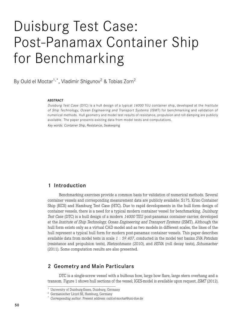
DTC is a single-screw vessel with a bulbous bow, large bow flare, large stern overhang and atransom. Figure 1 shows hull sections of the vessel; IGES-model is available upon request, ISMT (2012).
1 University of Duisburg-Essen, Duisburg, Germany2 Germanischer Lloyd SE, Hamburg, Germany* Corresponding author. Present address: [email protected]
50
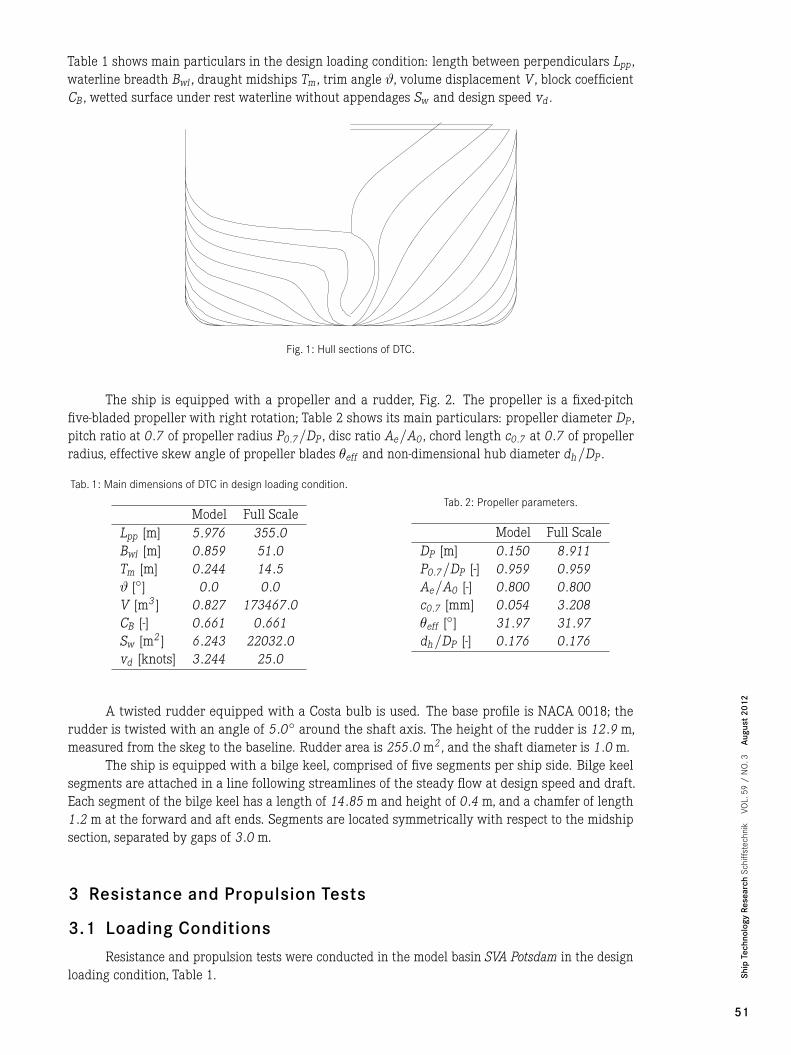
Table 1 shows main particulars in the design loading condition: length between perpendiculars Lpp ,waterline breadth Bwl , draught midships Tm , trim angle ϑ, volume displacement V , block coefficientCB , wetted surface under rest waterline without appendages Sw and design speed vd .
Fig. 1: Hull sections of DTC.
The ship is equipped with a propeller and a rudder, Fig. 2. The propeller is a fixed-pitchfive-bladed propeller with right rotation; Table 2 shows its main particulars: propeller diameter DP ,pitch ratio at 0 .7 of propeller radius P0 .7/DP , disc ratio Ae/A0 , chord length c0 .7 at 0 .7 of propellerradius, effective skew angle of propeller blades θeff and non-dimensional hub diameter dh/DP .
Tab. 1: Main dimensions of DTC in design loading condition.
Model Full ScaleLpp [m] 5 .976 355 .0Bwl [m] 0 .859 51 .0Tm [m] 0 .244 14 .5ϑ [◦] 0 .0 0 .0V [m3 ] 0 .827 173467 .0CB [-] 0 .661 0 .661Sw [m2 ] 6 .243 22032 .0vd [knots] 3 .244 25 .0
Tab. 2: Propeller parameters.
Model Full ScaleDP [m] 0 .150 8 .911P0 .7/DP [-] 0 .959 0 .959Ae/A0 [-] 0 .800 0 .800c0 .7 [mm] 0 .054 3 .208θeff [◦] 31 .97 31 .97dh/DP [-] 0 .176 0 .176
A twisted rudder equipped with a Costa bulb is used. The base profile is NACA 0018; therudder is twisted with an angle of 5 .0◦ around the shaft axis. The height of the rudder is 12 .9 m,measured from the skeg to the baseline. Rudder area is 255 .0 m2 , and the shaft diameter is 1 .0 m.
The ship is equipped with a bilge keel, comprised of five segments per ship side. Bilge keelsegments are attached in a line following streamlines of the steady flow at design speed and draft.Each segment of the bilge keel has a length of 14 .85 m and height of 0 .4 m, and a chamfer of length1 .2 m at the forward and aft ends. Segments are located symmetrically with respect to the midshipsection, separated by gaps of 3 .0 m.
3 Resistance and Propulsion Tests
3.1 Loading Conditions
Resistance and propulsion tests were conducted in the model basin SVA Potsdam in the designloading condition, Table 1.
51
Ship
Tech
nolo
gyRe
sear
chSc
hiff
stec
hnik
VOL.
59/
NO
.3Au
gust
2012
Fig. 2: Ship stern with rudder and propeller.
3.2 Open-Water Propeller Tests
Open-water propeller tests were performed at water kinematic viscosity 1 .044 · 10−6 m2 /sand density 998 .47 kg/m3 . Table 3 shows results, including non-dimensional thrust coefficient
KT = T/(ρD 4P n2 ) (1)
non-dimensional torque coefficientKQ = Q/(ρD 5
P n2 ) (2)
propeller efficiencyη0 = PT/PD (3)
and thrust loading coefficientCTh = 2T/(ρv2
a A0 ) (4)
The following definitions are used: T [N] is the propeller thrust, n [1/s] propeller rotationrate, Q [Nm] propeller torque, ρ [kg/m3 ] water density, PT = Tva [W] thrust power, PD = Qω [W]delivered power, va [m/s] propeller advance speed, A0 [m2 ] propeller disc area, ω = 2πn [rad/s]circular frequency of propeller rotation, and J = va/(nDP ) propeller advance ratio.
3.3 Resistance Tests
Resistance was measured at six forward speeds, corresponding to Froude numbers Fr =v/√
gLpp from 0 .172 to 0 .214 and full-scale advance speeds v from about 20 .0 to 25 .0 knots. Thehull was ballasted at the design draft 14 .5 m with zero trim, and was free in trim and sinkage. Testswere carried out at water kinematic viscosity νM = 1 .090 · 10−6 m2 /s and density 998 .8 kg/m3 .
Table 4 shows results referring to the model scale, including model speed vm [m/s], Froudenumber, Reynolds number Re = νM LppM/νM , total resistance RT [N] and its non-dimensional co-efficient CT = RT/(0 .5ρSwv2 ), frictional resistance RF [N] and its non-dimensional coefficientCF = RF/(0 .5ρSwv2 ), and non-dimensional wave resistance coefficient CW = RW/(0 .5ρSwv2 ).
The frictional resistance coefficient CF in Table 4 was calculated according to ITTC 1957 as
CF = 0 .075/(log10 Re − 2 .0)2 (5)
and the wave resistance coefficient was estimated as
CW = CT − (1 + k)CF (6)
52

Tab. 3: Results of open-water propeller tests.
J [-] KT [-] 10KQ [-] η0 [-] CTh [-]0 .00 0 .509 0 .713 0 .000 −0 .05 0 .492 0 .691 0 .057 500 .70 .10 0 .472 0 .667 0 .113 120 .10 .15 0 .450 0 .640 0 .168 50 .910 .20 0 .427 0 .613 0 .222 27 .170 .25 0 .403 0 .584 0 .275 16 .410 .30 0 .378 0 .554 0 .326 10 .690 .35 0 .353 0 .524 0 .375 7 .3330 .40 0 .327 0 .493 0 .423 5 .2100 .45 0 .302 0 .462 0 .468 3 .7940 .50 0 .276 0 .430 0 .511 2 .8120 .55 0 .250 0 .398 0 .551 2 .1070 .60 0 .225 0 .366 0 .586 1 .5880 .65 0 .199 0 .333 0 .617 1 .1960 .70 0 .172 0 .299 0 .642 0 .8940 .75 0 .145 0 .264 0 .657 0 .6570 .80 0 .118 0 .228 0 .656 0 .4670 .85 0 .089 0 .191 0 .630 0 .3120 .90 0 .058 0 .151 0 .553 0 .1830 .95 0 .026 0 .109 0 .361 0 .0741 .00 −0 .009 0 .065 −0 .209 −0 .022
The form factor k was found from a RANSE-CFD simulation for a double-body flow at the modelscale as k = 0 .094 (for reference, RANSE-CFD computed form factor for the full scale is k = 0 .145 ).
Tab. 4: Results of resistance model tests.
vM [m/s] Fr [-] Re × 10−6 [-] RT [N] RF [N] CT × 10 3 [-] CF × 10 3 [-] CW × 10 4 [-]1 .335 0 .174 7 .319 20 .34 17 .611 3 .661 3 .170 1 .9321 .401 0 .183 7 .681 22 .06 19 .229 3 .605 3 .142 1 .6721 .469 0 .192 8 .054 24 .14 20 .964 3 .588 3 .116 1 .7911 .535 0 .200 8 .415 26 .46 22 .713 3 .602 3 .092 2 .1941 .602 0 .209 8 .783 28 .99 24 .554 3 .623 3 .069 2 .6601 .668 0 .218 9 .145 31 .83 26 .431 3 .670 3 .047 3 .360
3.4 Propulsion Tests
Propulsion tests were carried out at the design draught with zero static trim, at the sameadvance speeds as the resistance tests described above. The model was free in trim and sinkage. Testswere conducted at water temperature 16 .8 ◦C , kinematic viscosity of water νM = 1 .090 · 10−6 m2 /sand water density ρM = 998 .8 kg/m3 .
The British method was used for friction deduction. The model was towed with various forwardspeeds; for each given forward speed, the propeller rotation rate was varied, and the residual forceacting from the carriage on the model (equal to the difference between the propeller thrust and hullresistance including suction force) was measured.
The self-propulsion point of the model, corresponding to the full scale, was found as the rotationrate at which this residual force is equal to the pre-defined difference of two forces: the total model
53
Ship
Tech
nolo
gyRe
sear
chSc
hiff
stec
hnik
VOL.
59/
NO
.3Au
gust
2012
resistance and the predicted total full-scale resistance, scaled to the model. This difference, called thefriction deduction, was calculated in model scale as
FD = 0 .5ρM SwM v2M (CTM − CT ) (7)
where index M denotes model scale. The total resistance coefficient CT is defined at the correspondingtemperature.
The values of the thrust and torque at the full scale self-propulsion point were defined byinterpolation over measurement results at the different rotation rates.
With the thus defined thrust T , torque Q and rotation rate n at the self-propulsion point, thrustand torque coefficients are calculated using equations (1) and (2), respectively. Starting with thusdefined KT , the corresponding advance ratio JT and the torque coefficient KQT are found from theopen-water propeller characteristics, Table 3, and then the effective wake fraction with respect tothrust can be calculated as
wT = 1 − JT DP/v (8)
as well as the relative rotative efficiency
ηR = KQT/KQ (9)
In a similar way, starting with the KQ value following from the interpolated torque Q , thecorresponding advance ratio JQ can be found from the open-water propeller characteristics, and theeffective wake fraction with respect to torque can be found as
wQ = 1 − JQ DP/v (10)
In addition to wT , wQ and ηR , Table 5 shows thrust deduction fraction t , hull efficiency ηH ,propulsive efficiency ηD , propeller efficiency η0 and the friction deduction FD [N], calculated usingeq. (7).
The thrust deduction fraction is calculated as
t = 1 − RT/T (11)
where RT is the predicted total resistance corresponding to the full scale.The hull efficiency is defined as
ηH = PE/PT = (1 − t)/(1 − w) (12)
where PE = Rv is the effective power.The propulsive efficiency is defined as
ηD = PE/PD (13)
Tab. 5: Results of propulsion model tests.
vM [m/s] t [-] wT [-] wQ [-] ηH [-] ηR [-] ηD [-] η0 [-] FDM [N]1 .335 0 .081 0 .264 0 .291 1 .249 0 .959 0 .720 0 .602 9 .4191 .401 0 .101 0 .279 0 .293 1 .247 0 .980 0 .729 0 .596 10 .2561 .469 0 .093 0 .277 0 .291 1 .255 0 .978 0 .734 0 .598 11 .1461 .535 0 .089 0 .281 0 .294 1 .266 0 .979 0 .739 0 .596 12 .0471 .602 0 .101 0 .277 0 .284 1 .245 0 .989 0 .730 0 .593 12 .9851 .668 0 .090 0 .275 0 .279 1 .255 0 .993 0 .738 0 .592 13 .947
54
4 Roll Damping Tests
4.1 Loading Conditions
Roll decay tests were carried out at HSVA with the same model. Two loading conditions wererealised, corresponding to the full-scale draughts of 12 .0 and 14 .0 m. Table 6 shows main parameters,including, in addition to those parameters shown in Table 1, the height KMt of the transversemetacentre above the keel, transverse metacentric height GMt , height KG of the centre of gravityabove the keel, natural period of small roll oscillations Tϕ, and dry longitudinal kxx , transversal kyy
and vertical kzz radii of inertia with respect to the centre of gravity.
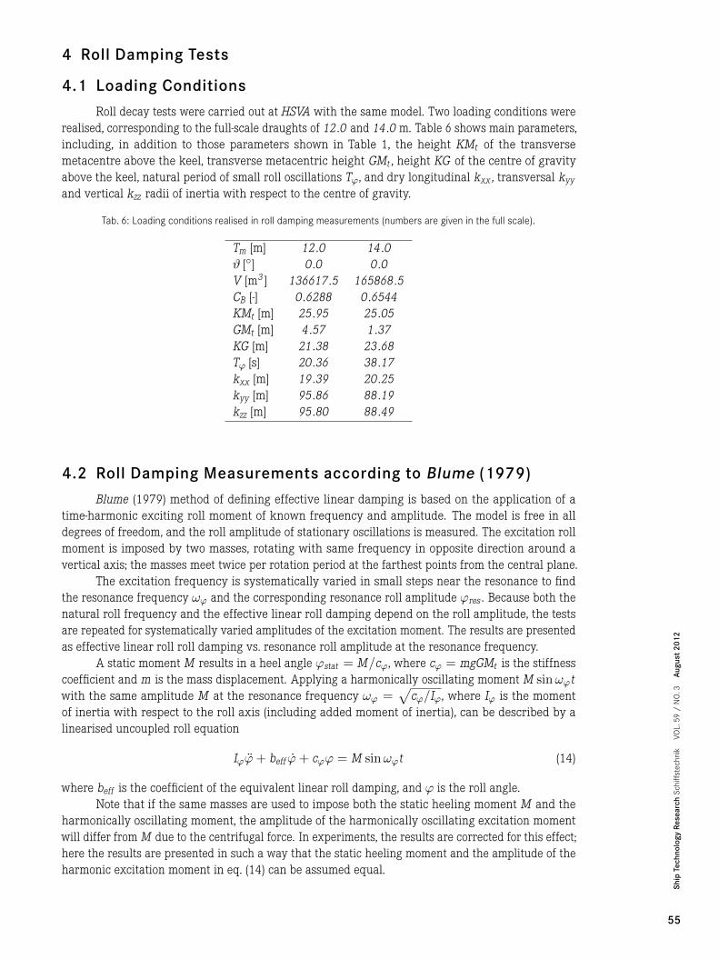
Tab. 6: Loading conditions realised in roll damping measurements (numbers are given in the full scale).
Tm [m] 12 .0 14 .0ϑ [◦] 0 .0 0 .0V [m3 ] 136617 .5 165868 .5CB [-] 0 .6288 0 .6544KMt [m] 25 .95 25 .05GMt [m] 4 .57 1 .37KG [m] 21 .38 23 .68Tϕ [s] 20 .36 38 .17kxx [m] 19 .39 20 .25kyy [m] 95 .86 88 .19kzz [m] 95 .80 88 .49
4.2 Roll Damping Measurements according to Blume (1979)
Blume (1979) method of defining effective linear damping is based on the application of atime-harmonic exciting roll moment of known frequency and amplitude. The model is free in alldegrees of freedom, and the roll amplitude of stationary oscillations is measured. The excitation rollmoment is imposed by two masses, rotating with same frequency in opposite direction around avertical axis; the masses meet twice per rotation period at the farthest points from the central plane.
The excitation frequency is systematically varied in small steps near the resonance to findthe resonance frequency ωϕ and the corresponding resonance roll amplitude ϕres . Because both thenatural roll frequency and the effective linear roll damping depend on the roll amplitude, the testsare repeated for systematically varied amplitudes of the excitation moment. The results are presentedas effective linear roll roll damping vs. resonance roll amplitude at the resonance frequency.
A static moment M results in a heel angle ϕstat = M/cϕ, where cϕ = mgGMt is the stiffnesscoefficient and m is the mass displacement. Applying a harmonically oscillating moment M sinωϕtwith the same amplitude M at the resonance frequency ωϕ =
√cϕ/Iϕ, where Iϕ is the moment
of inertia with respect to the roll axis (including added moment of inertia), can be described by alinearised uncoupled roll equation
Iϕϕ̈+ beff ϕ̇+ cϕϕ = M sinωϕt (14)
where beff is the coefficient of the equivalent linear roll damping, and ϕ is the roll angle.Note that if the same masses are used to impose both the static heeling moment M and the
harmonically oscillating moment, the amplitude of the harmonically oscillating excitation momentwill differ from M due to the centrifugal force. In experiments, the results are corrected for this effect;here the results are presented in such a way that the static heeling moment and the amplitude of theharmonic excitation moment in eq. (14) can be assumed equal.
55
Ship
Tech
nolo
gyRe
sear
chSc
hiff
stec
hnik
VOL.
59/
NO
.3Au
gust
2012
The resonance roll amplitude corresponding to eq. (14) is
ϕres =Mbeff
√Iϕcϕ
(15)
and thereforeϕstat/ϕres = beff/
√Iϕcϕ (16)
orbeff =
ϕstat
ϕres
cϕωϕ
(17)
thus the ratio ϕstat/ϕres can also be used to describe the effective linear damping coefficient.Roll damping was measured at three forward speeds of the model, 0 .0 , 0 .8 and 1 .47 m/s,
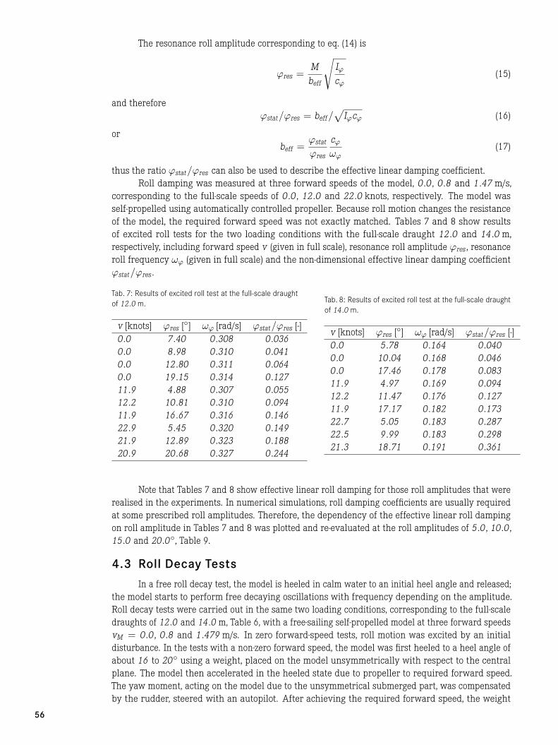
corresponding to the full-scale speeds of 0 .0 , 12 .0 and 22 .0 knots, respectively. The model wasself-propelled using automatically controlled propeller. Because roll motion changes the resistanceof the model, the required forward speed was not exactly matched. Tables 7 and 8 show resultsof excited roll tests for the two loading conditions with the full-scale draught 12 .0 and 14 .0 m,respectively, including forward speed v (given in full scale), resonance roll amplitude ϕres , resonanceroll frequency ωϕ (given in full scale) and the non-dimensional effective linear damping coefficientϕstat/ϕres .
Tab. 7: Results of excited roll test at the full-scale draughtof 12 .0 m.
v [knots] ϕres [◦] ωϕ [rad/s] ϕstat/ϕres [-]0 .0 7 .40 0 .308 0 .0360 .0 8 .98 0 .310 0 .0410 .0 12 .80 0 .311 0 .0640 .0 19 .15 0 .314 0 .12711 .9 4 .88 0 .307 0 .05512 .2 10 .81 0 .310 0 .09411 .9 16 .67 0 .316 0 .14622 .9 5 .45 0 .320 0 .14921 .9 12 .89 0 .323 0 .18820 .9 20 .68 0 .327 0 .244
Tab. 8: Results of excited roll test at the full-scale draughtof 14 .0 m.
v [knots] ϕres [◦] ωϕ [rad/s] ϕstat/ϕres [-]0 .0 5 .78 0 .164 0 .0400 .0 10 .04 0 .168 0 .0460 .0 17 .46 0 .178 0 .08311 .9 4 .97 0 .169 0 .09412 .2 11 .47 0 .176 0 .12711 .9 17 .17 0 .182 0 .17322 .7 5 .05 0 .183 0 .28722 .5 9 .99 0 .183 0 .29821 .3 18 .71 0 .191 0 .361
Note that Tables 7 and 8 show effective linear roll damping for those roll amplitudes that wererealised in the experiments. In numerical simulations, roll damping coefficients are usually requiredat some prescribed roll amplitudes. Therefore, the dependency of the effective linear roll dampingon roll amplitude in Tables 7 and 8 was plotted and re-evaluated at the roll amplitudes of 5 .0 , 10 .0 ,15 .0 and 20 .0◦, Table 9.
4.3 Roll Decay Tests
In a free roll decay test, the model is heeled in calm water to an initial heel angle and released;the model starts to perform free decaying oscillations with frequency depending on the amplitude.Roll decay tests were carried out in the same two loading conditions, corresponding to the full-scaledraughts of 12 .0 and 14 .0 m, Table 6, with a free-sailing self-propelled model at three forward speedsvM = 0 .0 , 0 .8 and 1 .479 m/s. In zero forward-speed tests, roll motion was excited by an initialdisturbance. In the tests with a non-zero forward speed, the model was first heeled to a heel angle ofabout 16 to 20◦ using a weight, placed on the model unsymmetrically with respect to the centralplane. The model then accelerated in the heeled state due to propeller to required forward speed.The yaw moment, acting on the model due to the unsymmetrical submerged part, was compensatedby the rudder, steered with an autopilot. After achieving the required forward speed, the weight
56

Tab. 9: Coefficients ϕstat/ϕres of equivalent linear roll damping vs. roll amplitude and forward speed.
ϕres [◦] Tm = 12 .0 m Tm = 14 .0 mFr [-] ϕstat/ϕres [-] Fr [-] ϕstat/ϕres [-]
5 .0 0 .000 0 .030 0 .000 0 .0395 .0 0 .104 0 .055 0 .104 0 .0945 .0 0 .200 0 .147 0 .198 0 .19810 .0 0 .000 0 .046 0 .000 0 .04710 .0 0 .106 0 .088 0 .106 0 .11710 .0 0 .194 0 .171 0 .196 0 .29915 .0 0 .000 0 .081 0 .000 0 .06815 .0 0 .105 0 .130 0 .105 0 .15415 .0 0 .189 0 .202 0 .191 0 .32920 .0 0 .000 0 .137 0 .000 0 .10120 .0 0 .101 0 .181 0 .104 0 .20320 .0 0 .183 0 .238 0 .183 0 .374
was removed using a rope system, attached to the carriage, following the model, and the modelstarted free decaying oscillations. Yaw oscillations, excited due to yaw coupling with roll motion, werecontrolled with the rudder, and the forward speed was adjusted by controlling the propeller rotationrate. Both the rudder and propeller were steered with an autopilot.
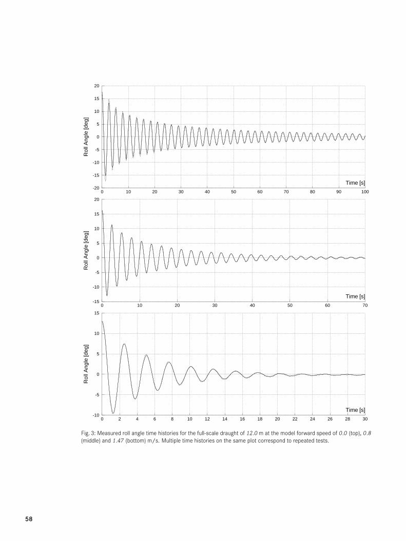
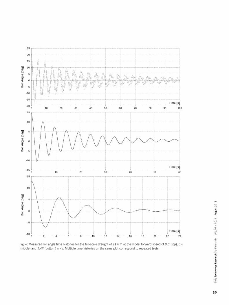
Figures 3 and 4 show measured roll decay time histories for the loading conditions with thefull-scale draughts 12 .0 and 14 .0 m, respectively.
For a homogeneous linearised decoupled roll equation
Iϕϕ̈+ beff ϕ̇+ cϕϕ = 0 (18)
with non-zero initial conditions, oscillatory solutions exist if the effective linear roll damping coefficientbeff is less than the critical roll damping bcr = 2
√Iϕcϕ. For ships, beff � bcr , and the solution is
a decaying oscillation, for which the influence of damping on the natural roll frequency ωϕ can beneglected, thus ωϕ =
√cϕ/Iϕ.
Different quantities can be used to describe roll decay, for example, roll decrement of nthorder, defined as
∆n = ϕa ,i/ϕa ,i+n (19)
i.e. the ratio of roll amplitudes ϕa separated by n roll periods. Most often, the first-order decrement∆1 (or simply ∆) is used, ∆ = ϕa ,i/ϕa ,i+1 ; from the solution of eq. (18),
∆ = exp [πbeff/(ωϕIϕ)] (20)
Natural logarithm of the first-order decrement ln∆, called logarithmic decrement, is alsofrequently used. Note that according to eq. (20),
δ ≡ ln∆ = πbeff/(ωϕIϕ) (21)
Another frequently used measure is the ratio of the effective linear roll damping coefficientbeff to the critical damping bcr ,
ζ ≡ beff/bcr = δ/(2π) (22)
often expressed as percentage. Remembering eq. (17), we can relate roll damping characteristics fromforced roll and free roll decay tests as
ζ = δ/(2π) = 0 .5ϕstat/ϕres = 0 .5beff/√
Iϕcϕ (23)
57
Ship
Tech
nolo
gyRe
sear
chSc
hiff
stec
hnik
VOL.
59/
NO
.3Au
gust
2012
Time [s]
Rol
lAng
le[d
eg]
0 10 20 30 40 50 60 70 80 90 100-20
-15
-10
-5
0
5
10
15
20
Time [s]
Rol
lAng
le[d
eg]
0 10 20 30 40 50 60 70-15
-10
-5
0
5
10
15
20
Time [s]
Rol
lAng
le[d
eg]
0 2 4 6 8 10 12 14 16 18 20 22 24 26 28 30-10
-5
0
5
10
15
Fig. 3: Measured roll angle time histories for the full-scale draught of 12 .0 m at the model forward speed of 0 .0 (top), 0 .8(middle) and 1 .47 (bottom) m/s. Multiple time histories on the same plot correspond to repeated tests.
58
Time [s]
Rol
lAng
le[d
eg]
0 10 20 30 40 50 60 70 80 90 100-20
-15
-10
-5
0
5
10
15
20
25
Time [s]
Rol
lAng
le[d
eg]
0 10 20 30 40 50 60-15
-10
-5
0
5
10
15
Time [s]
Rol
lAng
le[d
eg]
0 2 4 6 8 10 12 14 16 18 20 22 24-10
-5
0
5
10
15
Fig. 4: Measured roll angle time histories for the full-scale draught of 14 .0 m at the model forward speed of 0 .0 (top), 0 .8(middle) and 1 .47 (bottom) m/s. Multiple time histories on the same plot correspond to repeated tests.
59
Ship
Tech
nolo
gyRe
sear
chSc
hiff
stec
hnik
VOL.
59/
NO
.3Au
gust
2012
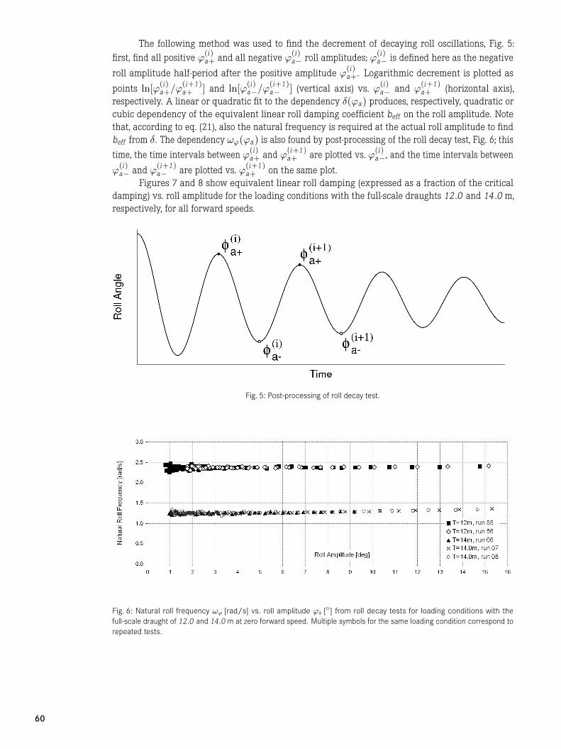
The following method was used to find the decrement of decaying roll oscillations, Fig. 5:first, find all positive ϕ(i)
a+ and all negative ϕ(i)a− roll amplitudes; ϕ(i)
a− is defined here as the negative
roll amplitude half-period after the positive amplitude ϕ(i)a+. Logarithmic decrement is plotted as
points ln[ϕ(i)a+/ϕ
(i+1)a+ ] and ln[ϕ
(i)a−/ϕ
(i+1)a− ] (vertical axis) vs. ϕ(i)
a− and ϕ(i+1)a+ (horizontal axis),
respectively. A linear or quadratic fit to the dependency δ(ϕa) produces, respectively, quadratic orcubic dependency of the equivalent linear roll damping coefficient beff on the roll amplitude. Notethat, according to eq. (21), also the natural frequency is required at the actual roll amplitude to findbeff from δ. The dependency ωϕ(ϕa) is also found by post-processing of the roll decay test, Fig. 6; this
time, the time intervals between ϕ(i)a+ and ϕ(i+1)
a+ are plotted vs. ϕ(i)a−, and the time intervals between
ϕ(i)a− and ϕ(i+1)
a− are plotted vs. ϕ(i+1)a+ on the same plot.
Figures 7 and 8 show equivalent linear roll damping (expressed as a fraction of the criticaldamping) vs. roll amplitude for the loading conditions with the full-scale draughts 12 .0 and 14 .0 m,respectively, for all forward speeds.
Fig. 5: Post-processing of roll decay test.
Fig. 6: Natural roll frequency ωϕ [rad/s] vs. roll amplitude ϕa [◦] from roll decay tests for loading conditions with thefull-scale draught of 12 .0 and 14 .0 m at zero forward speed. Multiple symbols for the same loading condition correspond torepeated tests.
60

Fig. 7: Equivalent linear roll damping as percentage of critical damping from model tests for loading condition with thefull-scale draught of 12 .0 m at model forward speeds of 0 .0 (top), 0 .8 (middle) and 1 .47 (bottom) m/s. Different symbolson one plot correspond to repeated tests.
61
Ship
Tech
nolo
gyRe
sear
chSc
hiff
stec
hnik
VOL.
59/
NO
.3Au
gust
2012

Fig. 8: Equivalent linear roll damping as percentage of critical damping from model tests for loading condition with thefull-scale draught of 14 .0 m at model forward speeds of 0 .0 (top), 0 .8 (middle) and 1 .47 (bottom) m/s. Different symbolson the same plot correspond to repeated runs.
62
5 Examples of Numerical Results
5.1 Resistance
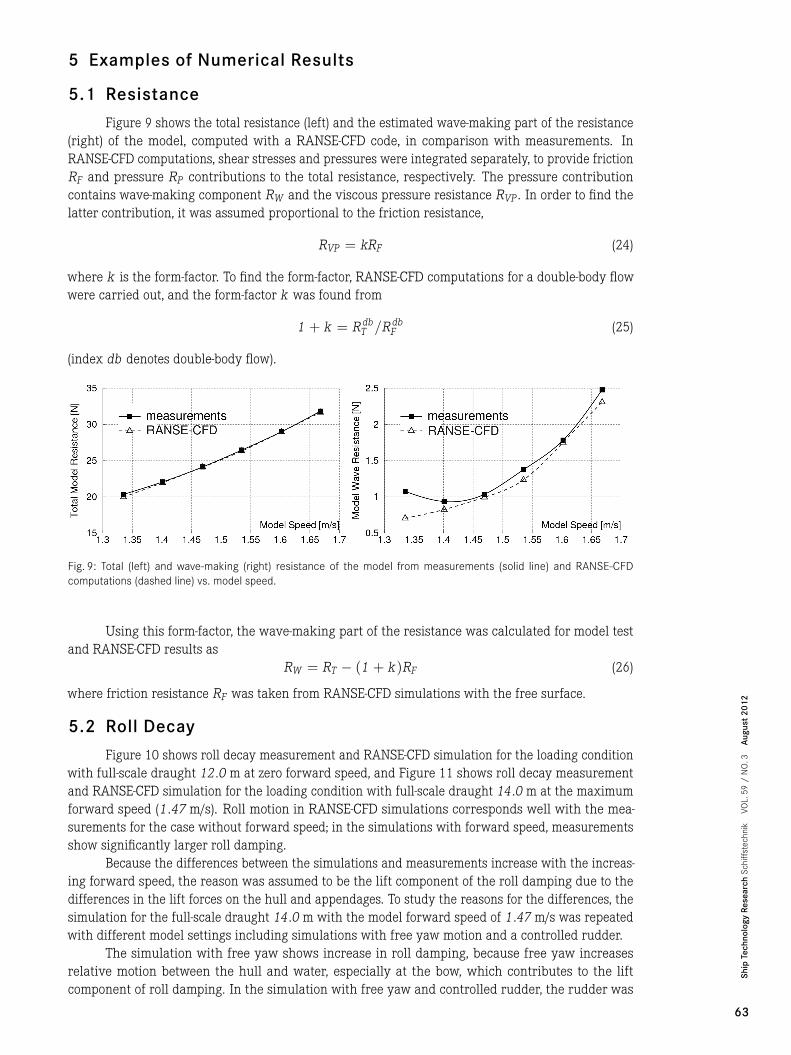
Figure 9 shows the total resistance (left) and the estimated wave-making part of the resistance(right) of the model, computed with a RANSE-CFD code, in comparison with measurements. InRANSE-CFD computations, shear stresses and pressures were integrated separately, to provide frictionRF and pressure RP contributions to the total resistance, respectively. The pressure contributioncontains wave-making component RW and the viscous pressure resistance RVP . In order to find thelatter contribution, it was assumed proportional to the friction resistance,
RVP = kRF (24)
where k is the form-factor. To find the form-factor, RANSE-CFD computations for a double-body flowwere carried out, and the form-factor k was found from
1 + k = R dbT /R db
F (25)
(index db denotes double-body flow).
Fig. 9: Total (left) and wave-making (right) resistance of the model from measurements (solid line) and RANSE-CFDcomputations (dashed line) vs. model speed.
Using this form-factor, the wave-making part of the resistance was calculated for model testand RANSE-CFD results as
RW = RT − (1 + k)RF (26)
where friction resistance RF was taken from RANSE-CFD simulations with the free surface.
5.2 Roll Decay
Figure 10 shows roll decay measurement and RANSE-CFD simulation for the loading conditionwith full-scale draught 12 .0 m at zero forward speed, and Figure 11 shows roll decay measurementand RANSE-CFD simulation for the loading condition with full-scale draught 14 .0 m at the maximumforward speed (1 .47 m/s). Roll motion in RANSE-CFD simulations corresponds well with the mea-surements for the case without forward speed; in the simulations with forward speed, measurementsshow significantly larger roll damping.
Because the differences between the simulations and measurements increase with the increas-ing forward speed, the reason was assumed to be the lift component of the roll damping due to thedifferences in the lift forces on the hull and appendages. To study the reasons for the differences, thesimulation for the full-scale draught 14 .0 m with the model forward speed of 1 .47 m/s was repeatedwith different model settings including simulations with free yaw motion and a controlled rudder.
The simulation with free yaw shows increase in roll damping, because free yaw increasesrelative motion between the hull and water, especially at the bow, which contributes to the liftcomponent of roll damping. In the simulation with free yaw and controlled rudder, the rudder was
63
Ship
Tech
nolo
gyRe
sear
chSc
hiff
stec
hnik
VOL.
59/
NO
.3Au
gust
2012

geometrically modelled and able to move. To simulate rudder forces accurately, propeller race wasalso modelled by longitudinal momentum sources, distributed in the propeller disc. The steeringof the rudder angle was done according to the rudder angle time history from the model test. Thissimulation shows significantly larger roll damping than in the simulation without rudder and withrestrained yaw.
This study shows that lift forces on the hull and especially on the rudder can produce asignificant contribution to roll damping with forward speed. The remaining differences between thesimulations and model tests require further study.
Fig. 10: Roll decay measurement and RANSE-CFD simulation for the loading condition with full-scale draught 12 .0 m at zeroforward speed.
Fig. 11: Roll decay measurement and RANSE-CFD simulation for the loading condition with full-scale draught 14 .0 m at themaximum model forward speed (1 .47 m/s).
ReferencesBlume, P. (1979). Experimentelle Bestimmung von Koeffizienten der wirksamen Rolldämpfung und ihre Anwendung zu Abschätzung
extremer Rollwinkel. Schiffstechnik, 26ISMT (2012). http://www.uni-due.de/ISMT/. Institute of Ship Technology, Ocean Engineering Project BestRollTransport Systems,
University Duisburg-EssenNietzschmann, T. (2010). Widerstands- und Propulsionsversuch für das Modell eines Containerschiffes. SVA Potsdam Model BasinSchumacher, A. (2011). Rolldämpfungsversuche mit dem Modell eines groß en Containerschiffes. The Hamburg Ship Model Basin
64