Dual-probe decoherence microscopy: probing pockets of coherence in a decohering

environment

This article has been downloaded from IOPscience. Please scroll down to see the full text article.

2012 New J. Phys. 14 023013

(http://iopscience.iop.org/1367-2630/14/2/023013)

Download details:

IP Address: 132.210.204.228

The article was downloaded on 08/02/2012 at 20:27

Please note that terms and conditions apply.

View the table of contents for this issue, or go to the journal homepage for more

Home Search Collections Journals About Contact us My IOPscience

T h e o p e n – a c c e s s j o u r n a l f o r p h y s i c s

New Journal of Physics

Dual-probe decoherence microscopy: probingpockets of coherence in a decohering environment

Jan Jeske1,2,3,6, Jared H Cole1,2,3,6, Clemens Muller4,5,Michael Marthaler2,3 and Gerd Schon2,3

1 Chemical and Quantum Physics, School of Applied Sciences,RMIT University, Melbourne 3001, Australia2 Institut fur Theoretische Festkorperphysik, Karlsruhe Institute of Technology,D-76128 Karlsruhe, Germany3 DFG-Center for Functional Nanostructures (CFN), D-76128 Karlsruhe,Germany4 Institut fur Theorie der Kondensierten Materie, Karlsruhe Institute ofTechnology, D-76128 Karlsruhe, Germany5 Departement de Physique, Universite de Sherbrooke, Sherbrooke, Quebec,J1K 2R1, CanadaE-mail: jan.jeske@rmit.edu.au and jared.cole@rmit.edu.au

New Journal of Physics 14 (2012) 023013 (26pp)Received 10 October 2011Published 6 February 2012Online at http://www.njp.org/doi:10.1088/1367-2630/14/2/023013

Abstract. We study the use of a pair of qubits as a decoherence probe of anontrivial environment. This dual-probe configuration is modelled by three two-level systems (TLSs), which are coupled in a chain in which the middle systemrepresents an environmental TLS. This TLS resides within the environment of thequbits and therefore its coupling to perturbing fluctuations (i.e. its decoherence)is assumed much stronger than the decoherence acting on the probe qubits. Westudy the evolution of such a tripartite system including the appearance of adecoherence-free state (dark state) and non-Markovian behaviour. We find thatall parameters of this TLS can be obtained from measurements of one of theprobe qubits. Furthermore, we show the advantages of two qubits in probingenvironments and the new dynamics imposed by a TLS that couples to two qubitsat once.

6 Authors to whom any correspondence should be addressed.

New Journal of Physics 14 (2012) 0230131367-2630/12/023013+26$33.00 © IOP Publishing Ltd and Deutsche Physikalische Gesellschaft

2

Contents

1. Introduction 22. The model and methods 43. Dynamics 7

3.1. A single qubit coupled to a two-level system . . . . . . . . . . . . . . . . . . . 73.2. Two qubits coupled to a two-level system . . . . . . . . . . . . . . . . . . . . 9

4. Probing a single two-level system with two qubits: parameter extraction 154.1. Weak decoherence regime—oscillating behaviour . . . . . . . . . . . . . . . . 154.2. Strong decoherence regime—decaying behaviour . . . . . . . . . . . . . . . . 17

5. Experimental realizations 176. Conclusion 18Acknowledgments 19Appendix A. Analytical understanding of the expectation values and their

Fourier transforms 19Appendix B. Calculation of the effective decay rate of a sum of decaying oscillations 22Appendix C. Hamiltonian eigenstates of the system 23References 24

1. Introduction

The loss of coherence (decoherence) of quantum bits (qubits) due to environmentalperturbations is an important obstacle on the way to large-scale quantum electronics andquantum computation. Such perturbations, at the same time, contain information about thesurrounding environment, which generates them. The idea of using qubits as probes oftheir environment has recently attracted interest [1–5] as an alternative application of qubittechnology where the effects of decoherence are used, rather than suppressed.

In general, when an environment acts on a qubit as a weakly coupled, fluctuating bath, theenvironmental effects can be simply expressed as a relaxation and an excitation rate as well asa pure dephasing rate. The decoherence process becomes much more complex when a qubitcouples to any component of an environment strongly enough such that quantum mechanicallevels within the environment need to be taken into account. In many systems, such partiallycoherent ‘pockets’ are observed in the environment. Examples include two-level fluctuators insuperconducting devices [6–11], impurity spins in semiconductors [12–16] and single-moleculemagnets [17–19] such as 8Fe and ferritin. Valuable information about the quantum mechanicalnature of the environment may be obtained using qubits as a direct environmental probe, withpotentially high sensitivity and high spatial resolution [2].

The concept of qubit probes has already been used to realize a nano-magnetometer usingnitrogen-vacancy (NV) centres in diamond attached to the end of atomic force microscopecantilevers [20–24]. In this case, the Zeeman splitting of electronic levels within the NVcentre is optically probed to provide a direct measure of the local magnetic field to nanometreresolution [24]. Additional information that one may obtain from the decoherence processes hasalso been studied [25, 26] in this context of classically fluctuating fields.

New Journal of Physics 14 (2012) 023013 (http://www.njp.org/)

3

Qubit 1 Qubit 2

2ωq

2ωt = 2ωq + 2δTLS

g1 g2

2ωq

coupling to bath

y

A

B

∝ Γ1 ∝ Γϕ

∝ (g1 − g2) or (g21 − g22)

3ωq + δ

ωq +√δ2 + 4g2

ωq + δωq −

√δ2 + 4g2

− ωq +√δ2 + 4g2

− ωq − δ− ωq −

√δ2 + 4g2

− 3ωq − δ

energy

|8〉

|7〉|6〉|5〉|4〉|3〉|2〉

|1〉

C

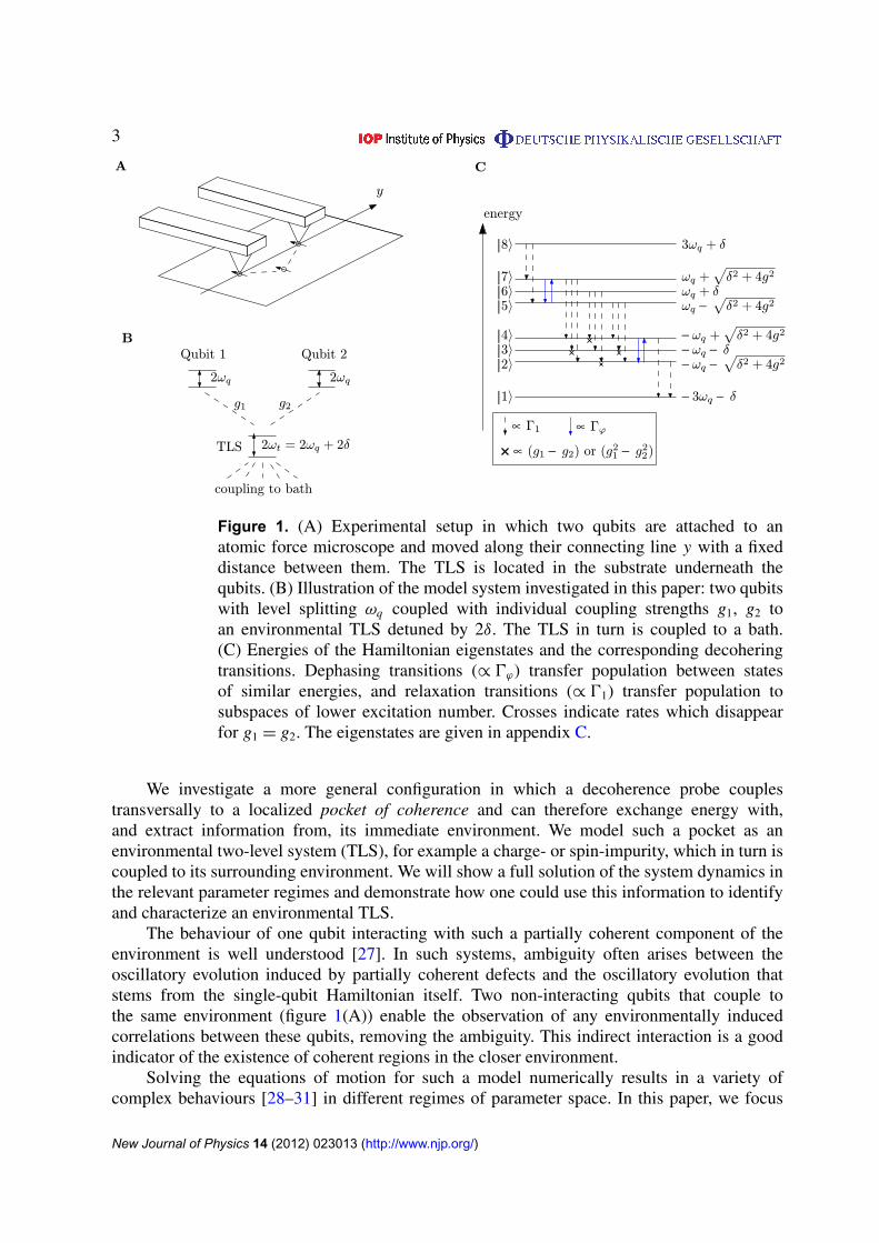
Figure 1. (A) Experimental setup in which two qubits are attached to anatomic force microscope and moved along their connecting line y with a fixeddistance between them. The TLS is located in the substrate underneath thequbits. (B) Illustration of the model system investigated in this paper: two qubitswith level splitting ωq coupled with individual coupling strengths g1, g2 toan environmental TLS detuned by 2δ. The TLS in turn is coupled to a bath.(C) Energies of the Hamiltonian eigenstates and the corresponding decoheringtransitions. Dephasing transitions (∝ 0ϕ) transfer population between statesof similar energies, and relaxation transitions (∝ 01) transfer population tosubspaces of lower excitation number. Crosses indicate rates which disappearfor g1 = g2. The eigenstates are given in appendix C.

We investigate a more general configuration in which a decoherence probe couplestransversally to a localized pocket of coherence and can therefore exchange energy with,and extract information from, its immediate environment. We model such a pocket as anenvironmental two-level system (TLS), for example a charge- or spin-impurity, which in turn iscoupled to its surrounding environment. We will show a full solution of the system dynamics inthe relevant parameter regimes and demonstrate how one could use this information to identifyand characterize an environmental TLS.

The behaviour of one qubit interacting with such a partially coherent component of theenvironment is well understood [27]. In such systems, ambiguity often arises between theoscillatory evolution induced by partially coherent defects and the oscillatory evolution thatstems from the single-qubit Hamiltonian itself. Two non-interacting qubits that couple tothe same environment (figure 1(A)) enable the observation of any environmentally inducedcorrelations between these qubits, removing the ambiguity. This indirect interaction is a goodindicator of the existence of coherent regions in the closer environment.

Solving the equations of motion for such a model numerically results in a variety ofcomplex behaviours [28–31] in different regimes of parameter space. In this paper, we focus

New Journal of Physics 14 (2012) 023013 (http://www.njp.org/)

4

on solving the system analytically in key regimes and then use these analytical solutions tounderstand the more general behaviour numerically.

Our model of two qubits coupled to a common environmental TLS has many similaritiesto the well-studied problem of two qubits coupled to a quantum harmonic oscillator.This classic Tavis–Cummings model has been widely investigated for its use in quantuminformation processing and studying atom–photon interactions. Interpreted in this context, ourresults complement a variety of physical effects that appear in the Tavis–Cummings model,including dispersive coupling [32–37], ultra-strong coupling [38–40] and entanglement birthand death [41–44]. It is natural that similar effects appear in both systems due to their formalequivalence within the single-excitation subspace. There are, however, important physicaldifferences, as an environmental TLS is typically more localized in space than a quantumharmonic oscillator and the symmetry of the TLS allows a more general coupling to itsenvironment.

After introducing the theoretical model in section 2, we present a general analysis of thesystem in section 3: in the weak decoherence regime, we find an oscillation of energy betweenthe qubits, i.e. an environmentally mediated coupling. We find a decoherence-free state (darkstate), which leads to the formation of stray entanglement between the qubits in the decoherenceprocess independent of the decoherence strength of the TLS. In our analytical solutions wefind a clear threshold between oscillations and decay. In order to clarify what constitutes anenvironmental pocket of coherence it is shown that the same threshold divides Markovian fromnon-Markovian system dynamics. We define an effective decay rate of the qubit dynamics,which turns out to have a linear dependence on the decoherence rates of the TLS in the weakdecoherence regime and a roughly inverse dependence in the strong decoherence regime. Insection 4, we interpret our results in the context of dual-probe microscopy and we find that inthe weak decoherence regime an environmental TLS can be fully characterized and located ina substrate. In the strong decoherence regime the TLS can only be located. Section 5 puts thetheoretical model in the context of present experimental qubit realizations.

2. The model and methods

In order to study how a qubit probe pair interacts with an environmental TLS, we constructa simplified model. Consider an experimental setup in which the two qubits are attached toan atomic force microscope such that they can be positioned precisely (with a fixed distancebetween them) on top of a scanned substrate which contains the TLS (figure 1(A)). At severalpositions the population of the excited state of the qubit is measured as a function of time. Ineach position of the cantilever the coupling strengths between the qubits and the TLS, g1 and g2,vary due to their relative position. We will give a detailed model of this variation in section 4.The full system Hamiltonian can be written as

Hsys = ωqσQ1z + ωqσ

Q2z + (ωq + δ)σ TLS

z + g1(σQ1x σ TLS

x + σ Q1y σ TLS

y )

+ g2(σQ2x σ TLS

x + σ Q2y σ TLS

y ), (1)

where σx , σy and σz are the respective Pauli operators which act on qubit 1 (Q1), qubit 2 (Q2) orthe TLS (TLS). The first two terms describe the two qubits which have the same level splittingof 2ωq , whereas the third term describes the TLS with a level splitting of 2(ωq + δ). Here, δ isthe relative detuning between qubits and TLS. The last two terms in equation (1) are transversalcoupling terms between each of the qubits and the TLS with the respective coupling strengths

New Journal of Physics 14 (2012) 023013 (http://www.njp.org/)

5

g1 and g2 and we introduce g =√

g21 + g2

2 for later simplicity. We focus on the specific caseof transversal coupling as we are particularly interested in direct energy exchange between thequbits and the TLS. Throughout this discussion, we use the terminology ‘qubit’ and ‘TLS’ todifferentiate between the fabricated and controllable two-state probes and the environmentalTLS of interest. For ease of notation, we will use the convention h = kB = 1.

As the system Hamiltonian Hsys is block-diagonal, the coherent evolution is limited tothe subspace states with equal excitation number. For the time evolution, we choose the statein which qubit 1 is in its excited state and the other two subsystems are in their ground state|Q1, Q2, TLS〉 = | ↑↓↓〉 as the system’s initial state. This is a state with a single excitationand therefore we can neglect the subspaces of higher excitation numbers in the followingcalculations.

A key advantage of probe qubits attached to a cantilever is that they can be calibrated whilelifted away from the sample. This allows the intrinsic decoherence of the probes themselves tobe accurately characterized. Once the probes are brought close to the sample, this intrinsicdecoherence defines a limit in the sensitivity for detecting features within the sample. For ourpurposes, an ideal qubit probe is one with a very long intrinsic decoherence time, as this providesa large dynamic range for sensing. We assume the intrinsic contribution to decoherence to besmall compared to the dynamics induced by the environmental TLS. Then we can ignore thiscontribution in what follows, i.e. assume that only the TLS is coupled to a fluctuating bath. Forits coupling to the environment, we take the operator

Hint = s B = (v⊥σ TLSx + v‖σ

TLSz )B, (2)

where v⊥ and v‖ are the transversal and longitudinal coupling strengths, respectively, and B isan operator acting on the bath. We assume a low-temperature bath ωq � T .

In most qubit architectures, the qubit’s level splitting is significantly larger than the otherenergy scales in the problem. Typically this is a requirement to obtain coherence over long timescales as well as adequate control over the quantum system. We therefore assume throughoutthis discussion that ωq � δ, g1, g2, T . Under this assumption we can neglect subspaces withmore than one excitation. A large ωq guarantees a clear separation of these subspaces in energywhile a low-temperature bath guarantees the absence of spontaneous excitations from the bath.In the limit of large ωq , one can often make an additional secular approximation, which wediscuss in detail later on. Breaking the assumption that the qubit’s level splitting is the largestenergy leads to the ultrastrong coupling regime, which is studied elsewhere [45].

We model the time evolution of the system’s reduced density matrix ρ using theBloch–Redfield equations [46, 47]. Using the eigenvectors |1〉 to |8〉 (given in appendix C)of Hsys as basis states, the Bloch–Redfield equations read element-wise:

ρnm = −iωnmρnm +∑n′m′

Rnmn′m′ρn′m′ (3)

with the Redfield tensor:

Rnmn′m′ := 3m′mnn′ + 3nn′m′m −

∑k

(3nkkn′δmm′ + 3kmm′kδnn′),

3nmn′m′ := snm sn′m′12C(ω = ωm′n′),

3nmn′m′ := snm sn′m′12C(ω = ωn′m′).

(4)

Here ρnm = 〈n|ρ|m〉 denotes the density matrix element at position n, m and ωnm := ωn − ωm

is the energy difference of the Hamiltonian eigenstates |n〉 and |m〉 of the system. The system

New Journal of Physics 14 (2012) 023013 (http://www.njp.org/)

6

operator that couples to the environment s is defined in Hint. In this approach the environmentis solely characterized through its spectral function

C(ω) :=∫

∞

−∞

dτ eiωτ〈B(τ )B(0)〉, (5)

where the bath operator B is taken in the interaction picture defined with respect to Hint. Thisspectral function, equation (5), is assumed to change slowly such that it does not change on thesmall scale of δ and g (but only on the much larger scale of 2ωq).

The transversal coupling to the low-temperature bath leads to unidirectional populationtransfers to states with lower excitation numbers, i.e. relaxation. These transfers appear in theBloch–Redfield equations as linear dependences of the time derivatives of certain diagonalelements of the system’s density matrix on other diagonal elements, each with a coefficient.These coefficients (i.e. relaxation transition rates) are all proportional to v2

⊥C(2ωq). For later

use we define a general relaxation rate due to the coupling of the TLS to the environment:

01 := v2⊥

C(2ωq). (6)

The longitudinal bath coupling leads to two processes: firstly, a loss of phase coherencebetween the states of the system, i.e. dephasing, which is mathematically represented bythe decay of off-diagonal elements in the density matrix; and secondly, a mutual populationtransfer between certain eigenstates [48] with the same excitation number: |2〉, |4〉 and |5〉, |7〉

(figure 1(C)). The corresponding decay rates and transition rates are all similarly proportionalto

0ϕ := v2‖C(0). (7)

An energy diagram of the eigenstates is depicted in figure 1(C) and all transitions are shown byarrows.

When the TLS is decoupled from the qubits (g1 = g2 = 0), 01 is the decay rate of thepopulation of its excited state and 20ϕ is the additional decay rate of its two off-diagonalelements, i.e. its relaxation and pure dephasing rates, respectively.

Comparing the resulting Bloch–Redfield equations with an approach assuming theLindblad equations [49, 50] with a phenomenological relaxation rate and dephasing rate onthe TLS, we find that the two sets of differential equations are equivalent when the followingtwo conditions are met. First the spectral function should not change on the scale of δ and g.As the second condition, one of the following three requirements has to be fulfilled: (i) the fullsecular approximation (explained in the next paragraph) is applied to both the Lindblad and theBloch–Redfield equations or (ii) we take only longitudinal TLS–bath coupling, i.e. v⊥ = 0, or(iii) we assume only transversal TLS–bath coupling, v‖ = 0, and choose an initial state which isconfined to the single-excitation subspace. In the case of equivalence, the two phenomenologicalrates in the Lindblad equations can be identified as our definitions 01 and 0ϕ .

The full secular approximation neglects all dependences between different elements ofthe system’s density matrix if at least one of them is an off-diagonal element. The necessaryand sufficient condition for this approximation is that the system’s level splittings and theirdifferences are large compared to the decoherence rates. Physically, this means assumingωq � g � 01, 0ϕ and ωq � |δ|, i.e. the TLS is somewhat coherent.

In the following sections, analytical solutions to the Bloch–Redfield equations in differentregimes are discussed. For δ = 0 these solutions are given in appendix A. The first solution weshow (appendix A.2) is obtained using the full secular approximation and is valid for what we

New Journal of Physics 14 (2012) 023013 (http://www.njp.org/)

7

call the weak decoherence regime, when the resulting decoherence rates are smaller than thecoupling strength g between the qubits and the TLS. We obtain two further analytical solutionsfor purely transversal (appendix A.3), i.e. v‖ = 0, and purely longitudinal (appendix A.4),i.e. v⊥ = 0, TLS–environment coupling. The combination of our particular initial state, the largeωq limit and v⊥v‖ = 0 allows us to solve the master equation without the secular approximation.This means that no assumption about the relative sizes of g and 01, 02 has to be made. Theselast two solutions are therefore also valid for strong decoherence, i.e. when the decoherencerates are bigger than the coupling strength g.

3. Dynamics

In this section we present the analytical solutions to the Bloch–Redfield equations for oursystem. We start the section by summarizing the results for a single qubit coupled to a TLS forlater comparison. Following this, in section 3.2 we study the behaviour of two qubits coupled toa TLS in detail.

3.1. A single qubit coupled to a two-level system

Before we study the more complicated case of two qubits, the dynamics of a single qubit coupledto an environmental TLS (see figure 2(A)) provides a clear overview of the relevant physics. Thisspecial case can be obtained from all solutions by setting g2 = 0 and tracing out the second qubit.Performing this on the Hamiltonian, equation (1), yields (for the corresponding eigenstates, seeappendix C)

H1q = ωqσQ1z + (ωq + δ)σ TLS

z + g1(σQ1x σ TLS

x + σ Q1y σ TLS

y ). (8)

A comparison with the results in this section will later allow us to distinguish phenomenawhich depend purely on the existence of two qubits and those which are due to qubit–TLScoupling in general. This section strongly depends on previous work [27], which is reproducedin our notation. As is observable, we consider the expectation value 〈σ Q1

z 〉 (which is proportionalto the qubit’s energy). Equivalently, one could use the probability of finding the qubit in theexcited state, Pexc =

12(〈σ

Q1z 〉 + 1).

Assuming weak decoherence (i.e. we take the full secular approximation in theBloch–Redfield equations) and no detuning δ = 0, one finds the expectation values as a functionof time:

〈σ Q1z 〉(t) = −1 + e−

012 t + e(−

012 −0ϕ)t cos [4g1 t] , (9)

〈σ TLSz 〉(t) = −1 + e−

012 t

− e(−012 −0ϕ)t cos [4g1 t] . (10)

The population oscillates between the qubit and the TLS (cf figure 2(B)) with the oscillationfrequency proportional to their transversal coupling strength. The oscillations decay on the timescale corresponding to the decoherence rates of the TLS.

Equivalently, we can consider the evolution in Fourier space, where the frequency and thedecay rate are equal to the position and width, respectively, of the corresponding frequency peak(for details see appendix A.5). In figure 2(C) the real part of the one-sided Fourier transformof 〈σ Q1

z 〉(t) is plotted as a function of detuning between the qubit and the TLS. The peak thatstarts at frequency 4g1 diminishes with increasing detuning, indicating a shift from oscillatory

New Journal of Physics 14 (2012) 023013 (http://www.njp.org/)

8

2ωq

2ωt = 2ωq + 2δTLS

coupling to bath

γ1

Qubit 1

A

B

C

Figure 2. (A) Illustration of the simplified model system of one qubit withlevel splitting ωq coupled with coupling strength g1 to an environmental TLSdetuned by δ. The TLS in turn is coupled to a bath. This system follows fromfigure 1(A) by setting g2 = 0. (B) Expectation values for the case of a singlequbit coupled to a TLS as a function of time for 01 = 0ϕ = 0.1g1; g2 = 0;δ = 0. (C) Real part of the one-sided Fourier transform of 〈σ Q1

z 〉(t) as a functionof detuning δ with 01 = 0ϕ = 0.1g1; g2 = 0. This is a numerical solution ofeither the Bloch–Redfield equations, where 01 and 0ϕ are the definitions givenby equations (6) and (7), or a numerical solution of the Lindblad equationswith phenomenological rates. Analytically we find the angular frequency of theoscillation: ωosc = 2

√δ2 + 4g2

1 , which is drawn as a dashed line. For details ofthe calculation, see section 3.1.

behaviour to pure exponential decay. The analytical solution for 〈σ Q1z 〉(t) with δ 6= 0 contains

complicated coefficients [27], but the frequency of the oscillation is simply ωosc = 2√

δ2 + 4g21 .

This corresponds to the level splitting between the hybridized states |2〉1q and |4〉1q (given inappendix C) and is plotted as a dashed line in figure 2(C). The oscillatory behaviour is describedby this one frequency, which corresponds to the standard ‘generalized Rabi frequency’ [51] from

New Journal of Physics 14 (2012) 023013 (http://www.njp.org/)

9

quantum optics. For large detuning δ the expectation value 〈σ Q1z 〉(t) is dominated by one purely

decaying term. A Taylor expansion for small g/δ on the corresponding decay rate shows thatthe rate vanishes with increasing δ/g as (01 + 40ϕ)g2/δ2

→ 0.So far, only weak decoherence on the TLS has been considered. We also wish to consider

the limit where the decoherence is stronger than the qubit–TLS coupling. Simplifying theequations to purely transversal bath coupling (v‖ = 0 ⇒ 0ϕ = 0), one finds analytical solutionsfor the system dynamics without the use of the secular approximation and therefore valid forstronger decoherence:

〈σ Q1z 〉(t) = −1 +

−64g21

µ2e−

t012 + 2 e−

t012

(−32g2

1 + 021

µ2cosh

[tµ

2

]+

01

µsinh

[tµ

2

]), (11)

where µ :=√

021 − 64g2

1 . From this expression, we see that as the decoherence rate 01 increasesrelative to the qubit–TLS coupling strength g1, the dynamics changes from oscillations to pureexponential decay. This becomes obvious by rewriting the hyperbolic cosine as

cosh

(1

2

√02

1 − 64g21 t

)=

cos(

12

√64g2

1 − 021 t

)for 8g1 > 01,

12

(e+··· + e−···

)for 8g1 < 01

(12)

and similarly for the hyperbolic sine functions. Therefore, we can identify the threshold betweenoscillations and decay in our approximations as precisely 01 = 8g1.

3.2. Two qubits coupled to a two-level system

Having reviewed the behaviour of a single qubit coupling to an environmental TLS, we nowconsider the behaviour of a dual-probe configuration. Such a system is of particular interestwhen there is no direct coupling between the qubits. This situation allows us to probe what wecall coherent pockets of the environment. When such a pocket is present in the environment,probing simultaneously with two qubits shows qualitatively different behaviour to the standardweakly coupled, Markovian environment, which would affect each qubit independently.

3.2.1. Mediated coupling between the qubits in the weak decoherence regime. We will firstshow how the coupling between qubits and TLS will mediate an effective interaction betweenthe two qubits themselves. For simplicity we initially consider δ = 0, i.e. both qubits areresonant with the TLS. In this case, and for the initial state chosen in section 2, the energy fromqubit 1 coherently oscillates between the two qubits via the excitation of the TLS (figure 3(A)).In contrast to the simpler case presented in section 3.1, the oscillations now show two distinctfrequencies, namely 4g and 2g. The smaller of the two frequencies corresponds to the oscillationof energy between the two qubits. The full analytical expression for 〈σ Q1

z 〉 can be found inappendix A.

Again the change in the system dynamics due to detuning δ 6= 0 can be understood bestby regarding the Fourier transform of the expectation value 〈σ Q1

z 〉(t). This yields a peak foreach term located at the corresponding frequency whose half-width at half-maximum (HWHM)is equal to the decay rate of the corresponding oscillatory component. Figure 3(B) shows theresult of a numerical solution of the Bloch–Redfield equations, with dashed lines indicating theanalytical expressions for the frequency shifts due to the detuning. With increasing detuningδ, the peak at frequency 2g splits into two different frequency peaks. The amplitude of the

New Journal of Physics 14 (2012) 023013 (http://www.njp.org/)

10

B

A

C

Figure 3. (A) Expectation values of both qubits and the TLS. The excitation isshifted from one qubit via the TLS to the other qubit and back. The parametersare chosen as: 01 = 0ϕ = 0.1g; g1 = g2; δ = 0. (B) Real part of the one-sidedFourier transform of 〈σ Q1

z 〉(t) as a function of detuning δ. Analytically wefind the three oscillation frequencies −δ +

√δ2 + 4g2, δ +

√δ2 + 4g2, 2

√δ2 + 4g2,

which are given by the dashed lines in the plot. The parameters are: 01 = 0ϕ =

0.1g; g1 = g2. (C) Time evolution of the expectation values for strong detuningδ = 5g; 01 = 0ϕ = 0.1g; g1 = g2. Even though the TLS is only minimallyexcited, the effective coupling mediated by it still leads to coherent exchangeof energy between the two qubits.

two high-frequency contributions diminishes with stronger detuning δ, while the amplitudeof the lower frequency peak increases. This means that for stronger detuning δ > g, theenergy oscillates between the qubits mainly at the lower frequency ωlow = |δ| −

√δ2 − 4g2. For

sufficiently strong detuning, the TLS is largely unpopulated during this process (figure 3(C)).This kind of off-resonant interaction with the TLS leads to an effective transversal coupling

between the qubits. This is the usual dispersive coupling term [32–35, 52], in this casedue to virtual excitation of the TLS. Performing a Taylor expansion for g/δ � 1 on boththe lower oscillation frequency ωlow and the decay rate of this oscillating term in the weakdecoherence solution with detuning yields ωlow ≈ 2g2/|δ| and γlow ≈ g2(01 + 120ϕ)/6δ2. Thelower frequency can here be interpreted as the effective coupling strength between the qubits

New Journal of Physics 14 (2012) 023013 (http://www.njp.org/)

11

ωlow = geff. This effective coupling approaches zero more slowly than the decay rate γlow as themagnitude of the detuning increases. The strongly detuned TLS therefore mediates an effectivetransversal coupling between the qubits with a weakened influence of the TLS’ decoherencerates. However, ultimately the effective coupling strength (i.e. the frequency of the oscillation)approaches zero for δ/g → ∞.

Here we see a fundamentally different behaviour as compared to a single qubit coupled to aTLS. The oscillations do not change to a pure decay for strong (but not yet infinite) detuning δ.Additionally, the frequency of these oscillations approaches zero much more slowly (∝ g/δ)than the decay rate of the single qubit (∝g2/δ2).

This result has important implications for future experimental designs involving severalqubits in a closely confined space. There the occurrence of an environmental TLS, whichcouples to two qubits at once, might have a realistic probability, especially in solid-state qubits.In that case the qubits are affected by the TLS over a wide range of detuning, causing effectivecoupling between the qubits.

3.2.2. Formation of stray entanglement. As we can see in figure 3(A), the steady state ofboth qubits is not their respective ground state. Rather, they decay into a state with a finiteprobability of finding them excited. This behaviour can be attributed to the existence of a so-called dark state in our system. The state |3〉 =

g2

g |↑↓↓〉−g1

g |↓↑↓〉 (appendix C) is an entangledstate of both qubits with the TLS in its ground state. The amplitudes of the two states (with therespective qubit excited) have a relative complex phase of π in the time evolution, which leads toa cancellation of the qubits’ influence on the TLS. In our system, this state is thus not influencedby decoherence and the system will remain in it for a long time (i.e. for the intrinsic decoherencetime of the qubits). This is simply a manifestation of the physics of super- and sub-radiance [53]due to the interfering pathways from the qubits to the TLS. Since our chosen initial state is astatistical mixture including the eigenstate |3〉, the steady state of the system will still includethis fraction of the dark state. The entanglement of the two qubits in the steady state depends onthe interplay of two things: the ‘concurrence’ [54] of the dark state by itself which is given byC = 2g1g2/g2 (i.e. a Bell state for g1 = g2) and the fraction of the dark state in the mixed steadystate. Taking both into consideration, we find the maximal ‘entanglement of formation’ [54] ofthe final state as E = 53%, which is reached for g1 = g2/

√3.

3.2.3. Threshold between weak and strong decoherence. When the decoherence rates of theTLS are stronger than the qubits–TLS coupling 01, 0ϕ > g the secular approximation (section 2)can no longer be fully applied. With increasing decoherence rates the dynamics of the threesubsystems changes from an oscillating behaviour to a pure decay. This behaviour is analogousto a single qubit coupled to a strongly decoherent TLS. In section 3.1 we saw that in this case thecrossover was defined by the point 01 = 8g1. For two qubits, the crossover between the weakand strong decoherence regimes is investigated numerically. For oscillations to occur betweenthe qubits and the environmental TLS there needs to be an instant in time in which the populationof the TLS is larger than both qubits combined. We therefore define the maximum value in theevolution:

M= maxt

{〈σ TLS

z 〉(t) −[〈σ Q1

z 〉(t) + 〈σ Q2z 〉(t)

]}(13)

as a measure of the strength of the oscillation. In the regime of strong decoherence, the energy ofthe qubits decays via the TLS to the environment and our defined measure is always zero. In the

New Journal of Physics 14 (2012) 023013 (http://www.njp.org/)

12

Figure 4. log10 of the oscillation strength M (equation (13)) as a function ofthe decoherence rates 01 and 0ϕ . The threshold between oscillations and decaycan be seen as a drop in the oscillation strength by four orders of magnitude.We solved the full Bloch–Redfield equations numerically (without the secularapproximation) and for simplicity we set g1 = g2 and δ = 0. The level splittingwas ωq = 1000g.

weak decoherence (i.e. oscillating) regime, the energy leaves the qubits and then partially returnsvia coherent oscillations from the TLS. This gives a positive value for the defined measure.Figure 4 is a logarithmic plot of this measure as a function of the two decoherence rates 01

and 0ϕ . There is a sudden drop in the oscillation strength to negligible values, marking a clearthreshold between the oscillating (weak decoherence) and the decaying (strong decoherence)regime. The oscillating regime (dark area) also marks precisely the parameter regime in whichthe full secular approximation is valid.

For purely transversal (respectively purely longitudinal) TLS–bath coupling v‖ = 0 ⇒

0ϕ = 0 (respectively v⊥ = 0 ⇒ 01 = 0) an analytical solution can be found. Analogous toequations (11) and (12), we find the analytical threshold between the strong and the weakdecoherence regime at the two points:

01 = 8g, 0ϕ = 0 and0ϕ = 4g, 01 = 0.

(14)

This corresponds to the point where the threshold in figure 4 crosses the two axes. The factor oftwo between 01 and 0ϕ stems directly from the definition of the rates (equations (6) and (7) asthey appear in the master equations, i.e. the off-diagonal elements of the uncoupled TLS-densitymatrix decay with a rate 20ϕ).

3.2.4. Markovianity. The coherent coupling to environmental states usually leads to non-Markovian [49, 55] dynamics in the system (excluding the environmental states). Using ourmodel, we can choose where to draw the system/environment boundary (see figure 5) andtherefore explore this behaviour in a systematic fashion. Regarding the TLS as part of thesystem, Markovian dynamics is assumed by default as this is a necessary condition to applythe Bloch–Redfield equations. However, tracing out the TLS we investigate the Markovianityof the two-qubit system.

New Journal of Physics 14 (2012) 023013 (http://www.njp.org/)

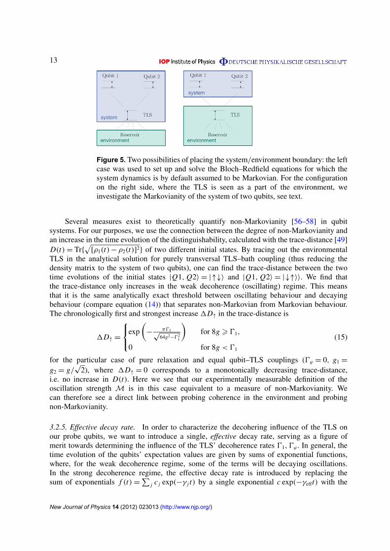
13

Figure 5. Two possibilities of placing the system/environment boundary: the leftcase was used to set up and solve the Bloch–Redfield equations for which thesystem dynamics is by default assumed to be Markovian. For the configurationon the right side, where the TLS is seen as a part of the environment, weinvestigate the Markovianity of the system of two qubits, see text.

Several measures exist to theoretically quantify non-Markovianity [56–58] in qubitsystems. For our purposes, we use the connection between the degree of non-Markovianity andan increase in the time evolution of the distinguishability, calculated with the trace-distance [49]D(t) = Tr{

√[ρ1(t) − ρ2(t)]2} of two different initial states. By tracing out the environmental

TLS in the analytical solution for purely transversal TLS–bath coupling (thus reducing thedensity matrix to the system of two qubits), one can find the trace-distance between the twotime evolutions of the initial states |Q1, Q2〉 = |↑↓〉 and |Q1, Q2〉 = |↓↑〉〉. We find thatthe trace-distance only increases in the weak decoherence (oscillating) regime. This meansthat it is the same analytically exact threshold between oscillating behaviour and decayingbehaviour (compare equation (14)) that separates non-Markovian from Markovian behaviour.The chronologically first and strongest increase 1D↑ in the trace-distance is

1D↑ =

exp

(−

π01√64g2−02

1

)for 8g > 01,

0 for 8g < 01

(15)

for the particular case of pure relaxation and equal qubit–TLS couplings (0ϕ = 0, g1 =

g2 = g/√

2), where 1D↑ = 0 corresponds to a monotonically decreasing trace-distance,i.e. no increase in D(t). Here we see that our experimentally measurable definition of theoscillation strength M is in this case equivalent to a measure of non-Markovianity. Wecan therefore see a direct link between probing coherence in the environment and probingnon-Markovianity.

3.2.5. Effective decay rate. In order to characterize the decohering influence of the TLS onour probe qubits, we want to introduce a single, effective decay rate, serving as a figure ofmerit towards determining the influence of the TLS’ decoherence rates 01, 0ϕ . In general, thetime evolution of the qubits’ expectation values are given by sums of exponential functions,where, for the weak decoherence regime, some of the terms will be decaying oscillations.In the strong decoherence regime, the effective decay rate is introduced by replacing thesum of exponentials f (t) =

∑j c j exp(−γ j t) by a single exponential c exp(−γefft) with the

New Journal of Physics 14 (2012) 023013 (http://www.njp.org/)

14

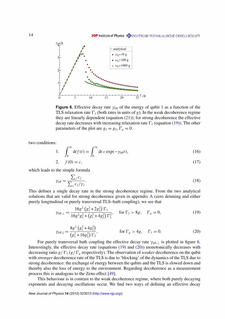
Figure 6. Effective decay rate γeff of the energy of qubit 1 as a function of theTLS relaxation rate 01 (both rates in units of g). In the weak decoherence regimethey are linearly dependent (equation (21)); for strong decoherence the effectivedecay rate decreases with increasing relaxation rate 01 (equation (19)). The otherparameters of the plot are g1 = g2, 0ϕ = 0.

two conditions:

1.

∫∞

0dt f (t) =

∫∞

0dt c exp(−γefft), (16)

2. f (0) = c, (17)

which leads to the simple formula

γeff =

∑j c j∑

j c j/γ j. (18)

This defines a single decay rate in the strong decoherence regime. From the two analyticalsolutions that are valid for strong decoherence given in appendix A (zero detuning and eitherpurely longitudinal or purely transversal TLS–bath coupling), we see that

γeff,⊥ =16g2

(g2

1 + 2g22

)01

16g2g21 +

(g2

1 + 4g22

)02

1

, for 01 > 8g, 0ϕ = 0, (19)

γeff,‖ =8g2

(g2

1 + 4g22

)(g2

1 + 16g22

)02

, for 0ϕ > 4g, 01 = 0. (20)

For purely transversal bath coupling the effective decay rate γeff,⊥ is plotted in figure 6.Interestingly, the effective decay rate (equations (19) and (20)) monotonically decreases withdecreasing ratio g/01 (g/0ϕ respectively). The observation of weaker decoherence on the qubitwith stronger decoherence rate of the TLS is due to ‘blocking’ of the dynamics of the TLS due tostrong decoherence: the exchange of energy between the qubits and the TLS is slowed down andthereby also the loss of energy to the environment. Regarding decoherence as a measurementprocess this is analogous to the Zeno effect [49].

This behaviour is in contrast to the weak decoherence regime, where both purely decayingexponents and decaying oscillations occur. We find two ways of defining an effective decay

New Journal of Physics 14 (2012) 023013 (http://www.njp.org/)

15

rate: describe either the decay of the envelope of the oscillations or the effective decay of theiraverage. For details, see [27] and appendix B. Here we use the decay of the average and find theeffective decay rate γeff to be linearly dependent on the relaxation rate 01:

γeff =1201 for 01 < 8g, 0ϕ < 4g. (21)

In the intermediate regime 2. 01/g < 8 and 1. 0ϕ/g < 4, where the lower bound is foundempirically, the oscillations are slow on the time scale of the decay. In this case, the first halfoscillation, the transmission of energy from the qubit into the TLS, dominates the behaviour,and the average decay rate does not reproduce the behaviour well. An effective decay rate isnot a good description of the dynamics in this regime and the apparent discontinuity in figure 6actually appears as a smooth transition in the time evolution of the qubits’ expectation value. Wehave also plotted three numerical calculations in figure 6 for different level splittings ωq (whileδ is always zero). As stated in section 2, the analytical result is obtained in the single-excitationsubspace which requires ωq � g1, g2, δ. We see excellent agreement between the analyticalsolution and the numerical solution of the full Bloch–Redfield equations for ωq & 1000g.

4. Probing a single two-level system with two qubits: parameter extraction

After studying the system and its dynamics in the previous sections, we now interpret the resultsin the context of decoherence microscopy. In particular, we focus on the ability to obtain the TLSparameters with a dual probe and compare it with a single-qubit probe. For this purpose, we onlyconsider the Fourier transform of the evolution of the qubits’ excited state population, as thisconveniently represents the parameters of interest.

Now we will give a more concrete form to the theoretical coupling parameters g1 andg2 from equation (1). If we assume that the coupling strengths depend on the distances d1

and d2 between the qubits and the TLS, as g j ∝ 1/d2j , and the qubits are moved along their

connecting line above the TLS in the substrate (see figure 1), then the coupling strengths behavecharacteristically as a function of the position y (figure 7).

4.1. Weak decoherence regime—oscillating behaviour

From an experimental point of view, the parameters δ, 01, 0ϕ of the environmental TLSand even the coupling strengths g1, g2 are in general unknown. We first consider the weakdecoherence regime when the qubits are close enough to the TLS (so that g � 01, 0ϕ). Thenthe obtained information of a measurement of 〈σ Q1

z 〉(t) is equivalent to a horizontal line infigure 3(B). The positions of the three peaks give the three frequencies in figure 3(B), i.e. thenecessary information to obtain the level splitting of the TLS δ and the qubits–TLS couplingstrength g uniquely. Measuring g at several positions above the sample allows the position ofthe environmental TLS to be obtained from the local minimum of g in figure 7, i.e. a single TLSin the substrate can be located.

The widths and heights of the peaks provide further parameters although they have verycomplicated dependences. In the case of resonance (δ = 0), however, we find three peaks thatallow an enormously simplified parameter extraction shown in figure 8. Experimentally, onesuch plot provides enough information to obtain all system parameters: g from the position ofthe peaks, 01 and 0ϕ from the HWHM and (having obtained these three parameters) g1 and g2

New Journal of Physics 14 (2012) 023013 (http://www.njp.org/)

16

Figure 7. Characteristic behaviour of the coupling strengths to the TLS in thesubstrate as a function of the position of the two qubits y (compare figure 1(A)).The distance between the peaks is controlled by the distance between the qubitsdqq . The width of the peaks is controlled by the height h above the sample.Here we chose dqq = 3h. The coupling strengths are normalized such that themaximum value is 1.

position HWHM heightpeak 1: 0 Γ1

2g41Γ1g4

peak 2: 2g Γ14 + Γϕ

2g21g22

(Γ14 +Γϕ)g4

peak 3: 4g Γ12 + Γϕ

g41(Γ1+2Γϕ)g4

⇒ g Γ1,Γϕ g1, g2

height

position

HWHM

Figure 8. Top: real part of the one-sided Fourier transform of 〈σ Q1z 〉(t) in the

weak decoherence regime (equation (A.4)) for δ = 0. Bottom: the table showshow the parameters could be obtained from a measurement of the plot above.

from the heights of the peaks. All system parameters can be obtained from one measurement ofthe time evolution of the excited state population of one of the probe qubits on resonance withthe TLS. To reach resonance experimentally the qubits could always be tuned to resonance withthe TLS, once δ is obtained as explained in the previous paragraph.

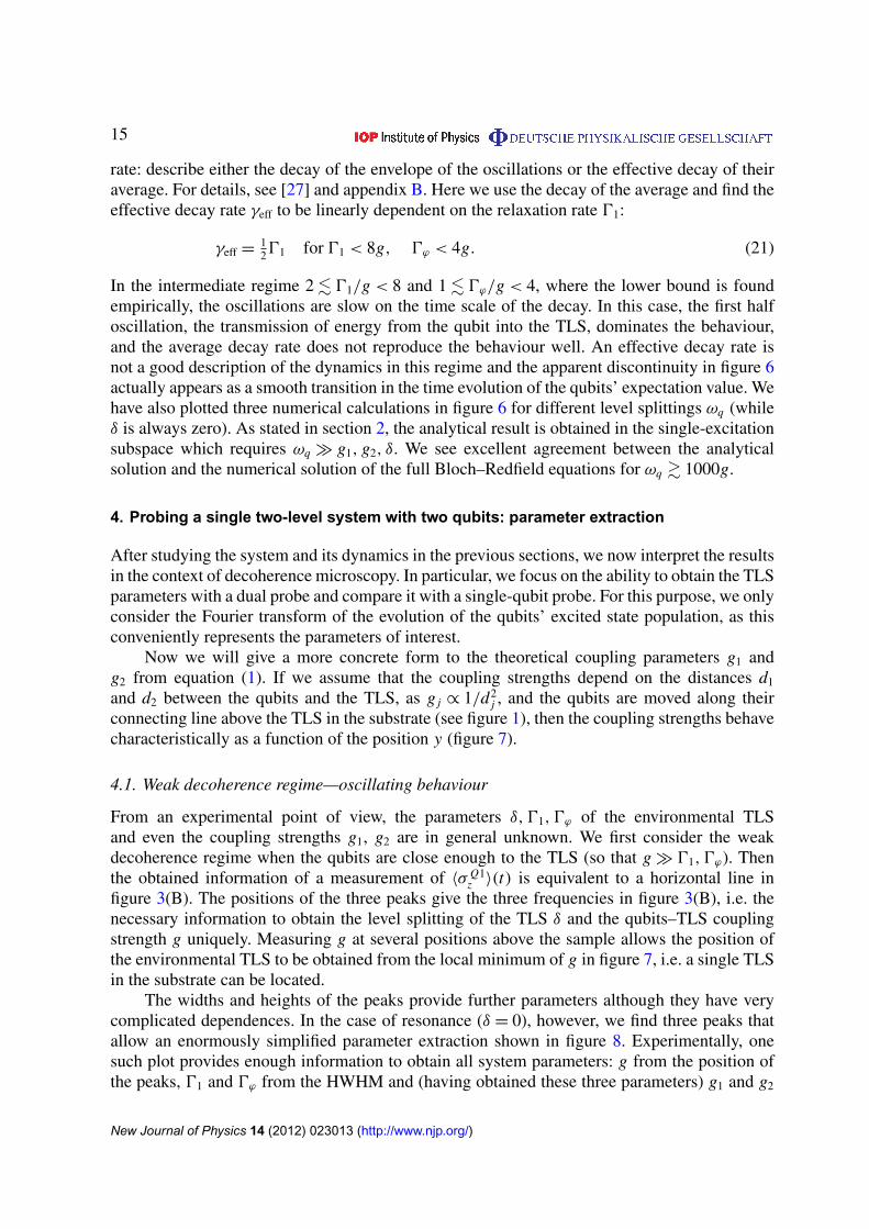
The major difference between the two qubits and a single qubit is the behaviour fordetuning to the TLS. While the single qubit is effectively decoupled by detuning, the addition ofa second qubit maintains an oscillating signal via the TLS-induced effective coupling betweenthe qubits. As a result, strong detuning and weak qubit–TLS coupling show two fundamentallydifferent behaviours and can be distinguished with two qubits (figure 9). The system is alsosensitive to TLS over a wider frequency range as the TLS-induced coupling decreases moreslowly with detuning.

New Journal of Physics 14 (2012) 023013 (http://www.njp.org/)

17

Figure 9. Expectation value of qubit 1 for the case of two qubits coupled to a TLSand g1 = g2 (top) and a single qubit coupled to a TLS (g2 = 0, bottom). Bothplots show two different cases: large detuning δ = 4.8g and weak qubit–TLScoupling g = 0.0501. For all plots 0ϕ = 0. These two different cases can only beclearly distinguished with two qubits.

Furthermore, the additional two lower frequencies in figure 3(B) that correspond tooscillations between the two qubits make it possible to obtain the detuning without changingthe level splitting of the qubits.

4.2. Strong decoherence regime—decaying behaviour

Scanning a substrate for isolated TLS one might find very different decoherence strengths foreach TLS, some of which might be fluctuating so strongly (or coupled so weakly) that nocoherent oscillations will occur even when the qubits are directly above it. In that case theabove technique of parameter extraction is no longer applicable. However, the TLS can still belocated (both with a single and two qubits) by monitoring the decay rate of the qubit at differentlocations along the y-axis in figure 1(A).

For pure relaxation the position dependence of the effective decay rate is shown infigures 10(A) (single-qubit probe) and 10(B) (two-qubit probes). The characteristic behaviourprovides the position of the TLS.

5. Experimental realizations

Although, in principle, any qubit architecture can be adapted for performing decoherencemicroscopy, in order to study microscopic pockets of coherence, atomic scale qubits withlong coherence times are ideal. In the solid state, this implies spin donors or defects, such assemiconductor donors [16, 59, 60] or colour centres in diamond [15, 20, 24].

As the NV centre in diamond is an experimentally established and well-investigatedsystem, we discuss the requirements to use these centres in a dual-probe configuration. Inrecent experiments the intrinsic decoherence of the NV centre is weak and dominated bythe dephasing [15, 20], which sets the sensitivity limit for probing environmental pockets ofcoherence. Isotopic purification of the diamond lattice [24] is currently being investigated forquantum computation and sensing purposes and will result in much longer coherence times,leading to a corresponding increase in sensitivity.

New Journal of Physics 14 (2012) 023013 (http://www.njp.org/)

18

A B

Figure 10. (A) Characteristic behaviour of the effective decay rate of the energyof a single qubit (g2 = 0) as a function of the position y. This plot is in thedecaying regime 01 = 10g1 and 0ϕ = 0. (B) Characteristic behaviour of theeffective decay rate of the energies of two qubits as a function of the positiony. This plot is in the decaying regime 01 = 10g1 and 0ϕ = 0.

In order to unambiguously identify coupling via the environment, we need to minimizeor eliminate coupling between the probes. This can be achieved in two configurations. Usingthe nuclear spin states of nitrogen within each NV centre as the qubit probes provides astrong electron–nuclear coupling to electron spins in the environment while minimizing theinter-qubit (nuclear–nuclear) coupling. For both a probe–TLS distance and probe separation of5 nm, we require T2 > 20 ms to reach the probe–TLS oscillation limit. Using current estimates[24, 61] for the dephasing channels due to 13C spins in the diamond lattice, this requires a 13Cconcentration below 0.03%. For this probe separation, the inter-probe coupling is a factor of1000 times smaller than the probe–TLS coupling and therefore provides no extra complicationto the analysis.

A second method of achieving strong probe–TLS coupling is to use a pair of NV centreswhose crystallographic orientation is such that the natural NV–NV coupling is eliminateddue to the angular dependence of the dipolar interaction. Although there are more seriousfabrication challenges with this configuration, the maximum dephasing required (T2 > 20 µs)is considerably less due to the strength of the electron–electron interaction. Such dephasingtimes are well within the range currently seen in experiments using NV centres [24].

In either of these configurations, detecting sample impurities with large magneticmoments such as single-molecule magnets (8Fe, ferritin) [17–19] is considerably easier,even with currently available intrinsic decoherence times. Depending on the backgroundfield configuration and qubit operating mode, these impurities will induce either dephasing-dominated or energy-exchange processes.

6. Conclusion

In this paper, we have investigated the concept of a dual-probe decoherence microscope. Usinga general model, we have studied the key characteristics of such a system analytically andnumerically. Mapping out the temporal dynamics of the qubit probes provides detailed informa-tion about a TLS, the simplest example of a pocket of coherence contained within the sample.

New Journal of Physics 14 (2012) 023013 (http://www.njp.org/)

19

In addition to the TLS’ level splitting and the coupling strengths to the probes, one can obtainits dephasing and relaxation rate, which implies the coupling strength to its surroundingenvironment and that environment’s constitution. A dual-probe configuration simplifies themeasurement process and increases sensitivity to detuned TLS. Furthermore, we have shownhow the oscillation amplitude of the environmentally mediated coupling between two probes islargely unaffected by detuning and decoherence of the mediating TLS, although the frequencyof oscillation still depends on detuning. The close relationship between environmentallymediated coupling and non-Markovian dynamics makes a dual-probe configuration ideal forprobing an environment’s potential to induce non-Markovian dynamics in a system as well asfor detecting the spatial extent and interrogate pockets of coherence which sit within a morecomplex environment.

Acknowledgments

We thank N Oxtoby, S Huelga and N Vogt for helpful discussions. This work was supportedby the CFN of Deutsche Forschungsgemeinschaft (DFG), the EU project SOLID and the USARO under contract no. W911NF-09-1-0336. We acknowledge support from DFG and the OpenAccess Publishing Fund of Karlsruhe Institute of Technology.

Appendix A. Analytical understanding of the expectation values and theirFourier transforms

In this appendix, we give the three analytical solutions each for no detuning δ = 0 (i.e. δ � g).As mentioned before, all three solutions were obtained in the subspace of one excitationplus the ground state with the assumption ωq � g1, g2. Furthermore, a low-temperature bathωq � T was assumed. First the secular approximation is explained, and then the three solutionsare given.

A.1. Matrix form of the master equation and the secular approximation

The Bloch–Refield equations, equation (3), can always be rewritten as a matrix multiplication.To do so, the elements of the density matrix need to be written in a vector. Here wechoose the particular order: all diagonal elements first and then all off-diagonal elements.To solve the equations the resulting Redfield tensor R, which is now a matrix, needs to bediagonalized.

The secular approximation means that for this diagonalization process, one can neglectoff-diagonal elements in the Redfield tensor R when there is a large difference between thecorresponding diagonal elements. In our chosen order we can regard separate blocks in theRedfield tensor (see below). The diagonal elements in the lower right block each have aterm −iω jk , whose magnitude is given by the energy difference of the two system states jand k. If these level splittings are large compared to the decoherence rates, then the two blockslinking diagonal and off-diagonal density matrix elements can be set to zero, i.e. the upper rightblock and the lower left block. If the differences of the energy differences ω jk − ωlm are alsolarge compared to the decoherence rates, then all off-diagonal Redfield tensor elements in thelower right block can also be set to zero. This is what we call the full secular approximation.

New Journal of Physics 14 (2012) 023013 (http://www.njp.org/)

20

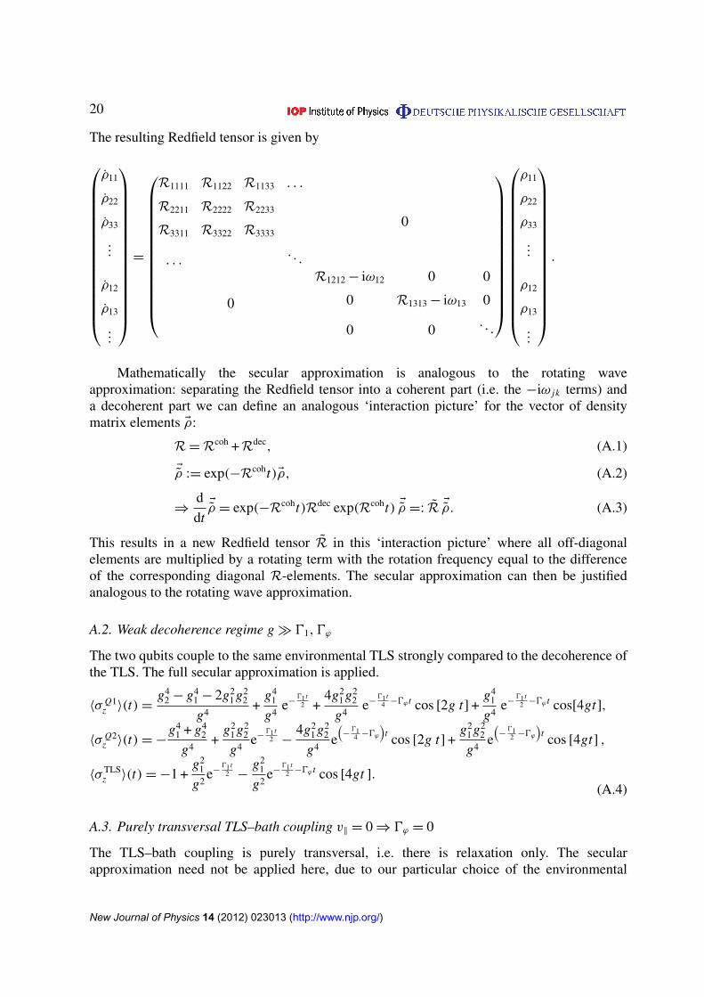
The resulting Redfield tensor is given by

ρ11

ρ22

ρ33

...

ρ12

ρ13

...

=

R1111 R1122 R1133 . . .

R2211 R2222 R2233

R3311 R3322 R3333

. . .. . .

0

0

R1212 − iω12 0 0

0 R1313 − iω13 0

0 0. . .

ρ11

ρ22

ρ33

...

ρ12

ρ13

...

.

Mathematically the secular approximation is analogous to the rotating waveapproximation: separating the Redfield tensor into a coherent part (i.e. the −iω jk terms) anda decoherent part we can define an analogous ‘interaction picture’ for the vector of densitymatrix elements Eρ:

R=Rcoh +Rdec, (A.1)

Eρ := exp(−Rcoht)Eρ, (A.2)

⇒d

dtEρ = exp(−Rcoht)Rdec exp(Rcoht) Eρ =: R Eρ. (A.3)

This results in a new Redfield tensor R in this ‘interaction picture’ where all off-diagonalelements are multiplied by a rotating term with the rotation frequency equal to the differenceof the corresponding diagonal R-elements. The secular approximation can then be justifiedanalogous to the rotating wave approximation.

A.2. Weak decoherence regime g � 01, 0ϕ

The two qubits couple to the same environmental TLS strongly compared to the decoherence ofthe TLS. The full secular approximation is applied.

〈σ Q1z 〉(t) =

g42 − g4

1 − 2g21g2

2

g4+

g41

g4e−

01t2 +

4g21g2

2

g4e−

01t4 −0ϕ t cos [2g t] +

g41

g4e−

01t2 −0ϕ t cos[4gt],

〈σ Q2z 〉(t) = −

g41 + g4

2

g4+

g21g2

2

g4e−

01t2 −

4g21g2

2

g4e

(−

014 −0ϕ

)t cos [2g t] +

g21g2

2

g4e

(−

012 −0ϕ

)t cos [4gt] ,

〈σ TLSz 〉(t) = −1 +

g21

g2e−

01t2 −

g21

g2e−

01t2 −0ϕ t cos [4gt ].

(A.4)

A.3. Purely transversal TLS–bath coupling v‖ = 0 ⇒ 0ϕ = 0

The TLS–bath coupling is purely transversal, i.e. there is relaxation only. The secularapproximation need not be applied here, due to our particular choice of the environmental

New Journal of Physics 14 (2012) 023013 (http://www.njp.org/)

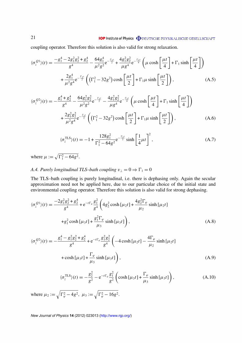
21

coupling operator. Therefore this solution is also valid for strong relaxation.

〈σ Q1z 〉(t) =

−g41 − 2g2

1g22 + g4

2

g4−

64g41

µ2g2e−

01t2 +

4g21g2

2

µg4e−

01t4

(µ cosh

[µt

4

]+ 01 sinh

[µt

4

])

+2g4

1

µ2g4e−

01t2

((02

1 − 32g2)

cosh

[µt

2

]+ 01µ sinh

[µt

2

]), (A.5)

〈σ Q2z 〉(t) = −

g41 + g4

2

g4−

64g21g2

2

µ2g2e−

01t2 −

4g21g2

2

µg4e−

01t4

(µ cosh

[µt

4

]+ 01 sinh

[µt

4

])

+2g2

1g22

µ2g4e−

01t2

((02

1 − 32g2)

cosh

[µt

2

]+ 01µ sinh

[µt

2

]), (A.6)

〈σ TLSz 〉(t) = −1 +

128g21

021 − 64g2

e−01t

2 sinh

[1

4µt

]2

, (A.7)

where µ :=√

021 − 64g2.

A.4. Purely longitudinal TLS–bath coupling v⊥ = 0 ⇒ 01 = 0

The TLS–bath coupling is purely longitudinal, i.e. there is dephasing only. Again the secularapproximation need not be applied here, due to our particular choice of the initial state andenvironmental coupling operator. Therefore this solution is also valid for strong dephasing.

〈σ Q1z 〉(t) =

−2g21g2

2 + g42

g4+ e−t0ϕ

g21

g4

(4g2

2 cosh [µ2t] +4g2

20ϕ

µ2sinh [µ2t]

+g21 cosh [µ3t] +

g210ϕ

µ3sinh [µ3t]

), (A.8)

〈σ Q2z 〉(t) = −

g41 − g2

1g22 + g4

2

g4+ e−t0ϕ

g21g2

2

g4

(−4 cosh [µ2t] −

40ϕ

µ2sinh [µ2t]

+ cosh [µ3t] +0ϕ

µ3sinh [µ3t]

), (A.9)

〈σ TLSz 〉(t) = −

g22

g2− e−t0ϕ

g21

g2

(cosh [µ3t] +

0ϕ

µ3sinh [µ3t]

), (A.10)

where µ2 :=√

02ϕ − 4g2, µ3 :=

√02

ϕ − 16g2.

New Journal of Physics 14 (2012) 023013 (http://www.njp.org/)

22

A.5. Fourier transform

The expressions in all expectation values contain constant and oscillating terms, with associateddecay rates. Terms of this form are more easily understood in the Fourier domain.

For measured signals of the form e−atcos[bt] the real part of its one-sided Fourier transformyields two Lorentzian peaks at the position of plus and minus the frequency b and with anHWHM which equals the decay rate a:

<

{∫∞

0e−iωt

[e−at cos(bt)

]dt

}=

a

2(a2 + (ω − b)2

) +a

2(a2 + (ω + b)2

) . (A.11)

Fitting such peaks allows us to experimentally obtain the frequency and decay rate in aprecise and simple way, as displayed in figure 8. Additionally, the close correspondence tothe parameters in the Fourier domain helps us to depict frequencies and decay rates at the sametime in figures 2(C) and 3(B).

Appendix B. Calculation of the effective decay rate of a sum of decaying oscillations

In the strong decoherence regime the oscillations are a sum of several exponentials∑j c j exp(−γ j t). To find one effective decay rate we can simply use equation (18). This

procedure is sensible when the different decay rates are not too far (i.e. not orders of magnitude)apart. Note that equation (18) can also be calculated from an integration:

c

γeff=

∑j c j

γeff=

∫∞

0

∑j

c j exp(−γ j t) dt =

∑j

c j

γ j. (B.1)

In the weak decoherence regime, on the other hand, we have additional oscillations forseveral terms, i.e. an expression of the form∑

j

c j exp(−γ j t) cos(ω j t), (B.2)

where some ω j might be zero and the cosine function might be replaced by a sine function forsome terms. In such a case (as, for example, displayed in figure 2(B) or 3(A)), one needs todecide to take either the average or the envelope of the oscillations. The effective decay rate ofthe average neglects the oscillating terms completely and can therefore become zero when thereare no purely decaying terms in the expression. On the other hand, the average is unambiguouswhile the upper envelope and the lower envelope can lead to different effective decay rates. Thisis the reason why the average was chosen in figure 6 for the weak decoherence (oscillating)regime.

The calculation of the average is performed by neglecting all oscillating terms andcalculating equation (18) from the rest. Numerically that is easily done by rewritingall oscillations in equation (B.2) as exponentials, which yields an expression of theform ∑

j

c j exp((−γ j + iω j)t). (B.3)

New Journal of Physics 14 (2012) 023013 (http://www.njp.org/)

23

Then all terms with a non-zero imaginary part in the exponential rate can be neglected and theeffective decay rate can be calculated as

average : γeff =

∑k ck∑

k ck/γk︸ ︷︷ ︸puredecays

, (B.4)

where k sums over all purely decaying terms.The calculation of the envelope is performed by setting all oscillations (including the

algebraic sign) to 1 (upper envelope) or −1 (lower envelope). Afterwards, equation (18) canbe applied to all terms. Numerically, that can easily be performed by taking the magnitude ofthe coefficients and real parts of the rates for all oscillating terms:

Upper envelope : γeff =

∑k ck +

∑l |cl |∑

k ck/γk +∑

l |cl |/γl, (B.5)

Lower envelope : γeff =

∑k ck −

∑l |cl |∑

k ck/γk −∑

l |cl |/γl, (B.6)

where k sums over all purely decaying terms and l sums over all oscillating terms. For the purelydecaying terms it is important not to take the magnitude of the coefficients in case negativecoefficients ck < 0 occur.

In principle, all terms with a non-zero imaginary part of the exponential rate areoscillations. However, when this imaginary part (which is the angular frequency of theoscillation) is smaller than the real part (which is the decay rate), this term decays stronglybefore the time period of one oscillation, i.e. the term looks like a pure (non-exponential) decay.For a numerical criterion whether a term should be categorized as oscillating or purely decaying,one could therefore measure the imaginary part relative to the real part for each individual term.However, for simplicity of the criterion we categorize, all terms with an imaginary part of theexponential rate below 0.1 (where g = 1) as purely decaying terms in our numerical calculationsfor figure 6. This is about one order of magnitude less than the decay rates plotted in figure 6.

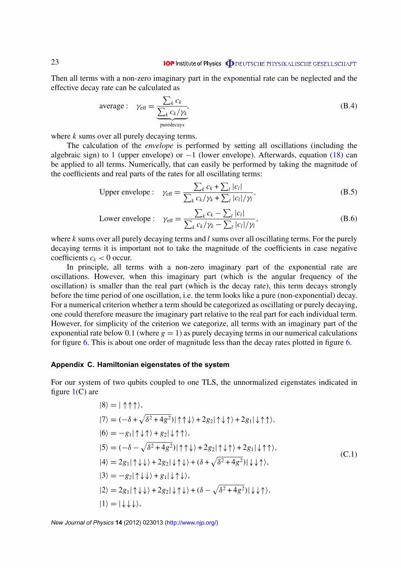
Appendix C. Hamiltonian eigenstates of the system

For our system of two qubits coupled to one TLS, the unnormalized eigenstates indicated infigure 1(C) are

|8〉 = | ↑↑↑〉,

|7〉 = (−δ +√

δ2 + 4g2)|↑↑↓〉 + 2g2|↑↓↑〉 + 2g1|↓↑↑〉,

|6〉 = −g1|↑↓↑〉 + g2|↓↑↑〉,

|5〉 = (−δ −√

δ2 + 4g2)|↑↑↓〉 + 2g2|↑↓↑〉 + 2g1|↓↑↑〉,

|4〉 = 2g1|↑↓↓〉 + 2g2|↓↑↓〉 + (δ +√

δ2 + 4g2)|↓↓↑〉,

|3〉 = −g2|↑↓↓〉 + g1|↓↑↓〉,

|2〉 = 2g1|↑↓↓〉 + 2g2|↓↑↓〉 + (δ −√

δ2 + 4g2)|↓↓↑〉,

|1〉 = |↓↓↓〉,

(C.1)

New Journal of Physics 14 (2012) 023013 (http://www.njp.org/)

24

where ↑ indicates an excited state and ↓ a ground state of the two qubits and the TLS in theorder |Q1, Q2, TLS〉.

Setting g2 = 0 and tracing out the second qubit yields the system of only one qubit coupledto a TLS discussed in section 3.1. Performing these operations on the above states, we find

|8〉 → |8〉1q = |↑↑〉,

|7〉 → |7〉1q = (−δ +√

δ2 + 4g2)|↑↓〉 + 2g1| ↓↑〉,

|6〉 → |6〉1q = −g1|↑↑〉,

|5〉 → |5〉1q = (−δ −√

δ2 + 4g2)|↑↓〉 + 2g1|↓↑〉,

|4〉 → |4〉1q = 2g1|↑↓〉 + (δ +√

δ2 + 4g2)|↓↑〉,

|3〉 → |3〉1q = g1|↓↓〉,

|2〉 → |2〉1q = 2g1|↑↓〉 + (δ −√

δ2 + 4g2)|↓↑〉,

|1〉 → |1〉1q = |↓↓〉.

(C.2)

Several states become equivalent:

|3〉1q = g1|1〉1q, (C.3)

|4〉1q =2g1

−δ +√

δ2 + 4g2|7〉1q, (C.4)

|5〉1q =−δ −

√δ2 + 4g2

1

2g1|2〉1q, (C.5)

|6〉1q = −g1|8〉1q . (C.6)

We therefore need (as one should expect) only four states to describe this reduced system.

References

[1] Shnirman A, Schon G, Martin I and Makhlin Y 2007 Josephson qubits as probes of 1/f noise ElectronCorrelation in New Materials and Nanosystems (NATO Science Series, number 241) (Berlin: Springer)pp 343–56

[2] Cole J H and Lloyd Hollenberg C L 2009 Scanning quantum decoherence microscopy Nanotechnology20 495401

[3] Chernobrod B M and Berman G P 2005 Spin microscope based on optically detected magnetic resonanceJ. Appl. Phys. 97 014903

[4] Weber J, Weis J, Hauser M and Von Klitzing K 2008 Fabrication of an array of single-electron transistors fora scanning probe microscope sensor Nanotechnology 19 375301

[5] de Sousa R 2009 Electron spin as a spectrometer of nuclear-spin noise and other fluctuations Electron SpinResonance and Related Phenomena in Low-Dimensional Structures (Topics in Applied Physics vol 115)ed M Fanciulli (Berlin: Springer) pp 183–220

[6] Martinis J M et al 2005 Decoherence in Josephson qubits from dielectric loss Phys. Rev. Lett. 95 210503[7] Neeley M, Ansmann M, Bialczak R C, Hofheinz M, Katz N, Lucero E, O’Connell A, Wang H, Cleland A N

and Martinis J M 2008 Process tomography of quantum memory in a Josephson-phase qubit coupled to atwo-level state Nature Phys. 4 523–6

New Journal of Physics 14 (2012) 023013 (http://www.njp.org/)

25

[8] Martin I, Bulaevskii L and Shnirman A 2005 Tunneling spectroscopy of two-level systems inside a Josephsonjunction Phys. Rev. Lett. 95 127002

[9] Bushev P, Mueller C, Lisenfeld J, Cole J H, Lukashenko A, Shnirman A and Ustinov A V 2010 Multiphotonspectroscopy of a hybrid quantum system Phys. Rev. B 82 134530

[10] Cole J H, Muller C, Bushev P, Grabovskij G J, Lisenfeld J, Lukashenko A, Ustinov A V and Shnirman A 2010Quantitative evaluation of defect-models in superconducting phase qubits Appl. Phys. Lett. 97 252501

[11] Lisenfeld J, Muller C, Cole J H, Bushev P, Lukashenko A, Shnirman A and Ustinov A V 2010 Rabispectroscopy of a qubit–fluctuator system Phys. Rev. B 81 100511

[12] Jelezko F, Gaebel T, Popa I, Gruber A and Wrachtrup J 2004 Observation of coherent oscillations in a singleelectron spin Phys. Rev. Lett. 92 076401

[13] Jelezko F, Gaebel T, Popa I, Domhan M, Gruber A and Wrachtrup J 2004 Observation of coherent oscillationof a single nuclear spin and realization of a two-qubit conditional quantum gate Phys. Rev. Lett. 93 130501

[14] Gaebel T et al 2006 Room-temperature coherent coupling of single spins in diamond Nature Phys. 2 408–13[15] Childress L, Gurudev Dutt M V, Taylor J M, Zibrov A S, Jelezko F, Wrachtrup J, Hemmer P R and Lukin M

D 2006 Coherent dynamics of coupled electron and nuclear spin qubits in diamond Science 314 281–5[16] Morello A et al 2010 Single-shot readout of an electron spin in silicon Nature 467 687–91[17] del Barco E, Hernandez J M, Tejada J, Biskup N, Achey R, Rutel I, Dalal N and Brooks J 2000 High-frequency

resonant experiments in f e8 molecular clusters Phys. Rev. B 62 3018–21[18] Awschalom D D, Smyth J F, Grinstein G, DiVincenzo D P and Loss D 1992 Macroscopic quantum tunneling

in magnetic proteins Phys. Rev. Lett. 68 3092–5[19] Tejada J, Zhang X X, del Barco E, Hernandez J M and Chudnovsky E M 1997 Macroscopic resonant tunneling

of magnetization in ferritin Phys. Rev. Lett. 79 1754–7[20] Balasubramanian G et al 2008 Nanoscale imaging magnetometry with diamond spins under ambient

conditions Nature 455 648–51[21] Maze J R et al 2008 Nanoscale magnetic sensing with an individual electronic spin in diamond Nature

455 644–7[22] Degen C L 2008 Scanning magnetic field microscope with a diamond single-spin sensor Appl. Phys. Lett.

92 243111[23] Taylor J M, Cappellaro P, Childress L, Jiang L, Budker D, Hemmer P R, Yacoby A, Walsworth R and Lukin

M D 2008 High-sensitivity diamond magnetometer with nanoscale resolution Nature Phys. 4 810–6[24] Balasubramanian G et al 2009 Ultralong spin coherence time in isotopically engineered diamond Nat. Mater.

8 383–7[25] Hall L T, Cole J H, Hill C D and Hollenberg L C L 2009 Sensing of fluctuating nanoscale magnetic fields

using nitrogen-vacancy centers in diamond Phys. Rev. Lett. 103 220802[26] Hall L T, Hill C D, Cole J H, Staedler B, Caruso F, Mulvaney P, Wrachtrup J and Lloyd Hollenberg C L

2010 Monitoring ion-channel function in real time through quantum decoherence Proc. Natl Acad. Sci.USA 107 18777–82

[27] Mueller C, Shnirman A and Makhlin Y 2009 Relaxation of Josephson qubits due to strong coupling to two-level systems Phys. Rev. B 80 94

[28] Oxtoby N P, Rivas A, Huelga S F and Fazio R 2009 Probing a composite spin-boson environment 2009 NewJ. Phys. 11 063028

[29] Yuan S, Katsnelson M I and De Raedt H 2008 Decoherence by a spin thermal bath: role of spin–spininteractions and initial state of the bath Phys. Rev. B 77 184301

[30] Emary C 2008 Quantum dynamics in nonequilibrium environments Phys. Rev. A 78 032105[31] Paladino E, Sassetti M, Falci G and Weiss U 2008 Characterization of coherent impurity effects in solid-state

qubits Phys. Rev. B 77 041303[32] Raimond J M, Brune M and Haroche S 2001 Manipulating quantum entanglement with atoms and photons in

a cavity Rev. Mod. Phys. 73 565–82[33] Sørensen A and Mølmer K 1999 Quantum computation with ions in thermal motion Phys. Rev. Lett.

82 1971–4

New Journal of Physics 14 (2012) 023013 (http://www.njp.org/)

26

[34] Zheng S-B and Guo G-C 2000 Efficient scheme for two-atom entanglement and quantum informationprocessing in cavity qed Phys. Rev. Lett. 85 2392–5

[35] Majer J et al 2007 Coupling superconducting qubits via a cavity bus Nature 449 443–7[36] Filipp S et al 2009 Two-qubit state tomography using a joint dispersive readout Phys. Rev. Lett. 102 200402[37] Niskanen A O, Nakamura Y and Tsai J-S 2006 Tunable coupling scheme for flux qubits at the optimal point

Phys. Rev. B 73 094506[38] Niemczyk T et al 2010 Circuit quantum electrodynamics in the ultrastrong-coupling regime Nature Phys.

6 772–6[39] Fink J M, Bianchetti R, Baur M, Goppl M, Steffen L, Filipp S, Leek P J, Blais A and Wallraff A 2009 Dressed

collective qubit states and the Tavis–Cummings model in circuit qed Phys. Rev. Lett. 103 083601[40] Casanova J, Romero G, Lizuain I, Garcıa-Ripoll J J and Solano E 2010 Deep strong coupling regime of the

Jaynes–Cummings model Phys. Rev. Lett. 105 263603[41] Yu T and Eberly J H 2009 Sudden death of entanglement Science 323 598–601[42] Yonac M, Yu T and Eberly J H 2006 Sudden death of entanglement of two Jaynes–Cummings atoms J. Phys.

B: At. Mol. Opt. Phys. 39 S621[43] Yu T and Eberly J H 2007 Negative entanglement measure, and what it implies J. Mod. Opt. 54 2289[44] Cole J H 2010 Understanding entanglement sudden death through multipartite entanglement and quantum

correlations J. Phys. A: Math. Theor. 43 135301[45] Ashhab S and Nori F 2010 Qubit-oscillator systems in the ultrastrong-coupling regime and their potential for

preparing nonclassical states Phys. Rev. A 81 042311[46] Bloch F 1957 Generalized theory of relaxation Phys. Rev. 105 1206–22[47] Redfield A G 1957 On the theory of relaxation processes IBM J. Res. Dev. 1 19–31[48] Boissonneault M, Gambetta J M and Blais A 2009 Dispersive regime of circuit QED: photon-dependent qubit

dephasing and relaxation rates Phys. Rev. A 79 013819[49] Breuer H-P and Petruccione F 2003 The Theory of Open Quantum Systems (Oxford: Oxford University Press)[50] Lindblad G 1976 On the generators of quantum dynamical semigroups Commun. Math. Phys. 48 119–30[51] Scully M O and Suhail Zubairy M 1999 Quantum Optics (Cambridge: Cambridge University Press)[52] Gerry C C and Knight P L 2005 Introductory Quantum Optics (Cambridge: Cambridge University Press)[53] Crubellier A, Liberman S, Pavolini D and Pillet P 1985 Superradiance and subradiance. I. Interatomic

interference and symmetry properties in three-level systems J. Phys. B: At. Mol. Phys. 18 3811[54] Wootters W K 1998 Entanglement of formation of an arbitrary state of two qubits Phys. Rev. Lett. 80 2245–8[55] Cui W, Rong Xi Z and Pan Y 2008 Optimal decoherence control in non-Markovian open dissipative quantum

systems Phys. Rev. A 77 032117[56] Breuer H-P, Laine E-M and Piilo J 2009 Measure for the degree of non-Markovian behavior of quantum

processes in open systems Phys. Rev. Lett. 103 210401[57] Rivas A, Huelga S F and Plenio M B 2010 Entanglement and non-Markovianity of quantum evolutions Phys.

Rev. Lett. 105 050403[58] Lu X-M, Wang X and Sun C P 2010 Quantum fisher information flow and non-Markovian processes of open

systems Phys. Rev. A 82 042103[59] Kane B E 1998 A silicon-based nuclear spin quantum computer Nature 393 133–7[60] de Sousa R, Delgado J D and Das Sarma S 2004 Silicon quantum computation based on magnetic dipolar

coupling Phys. Rev. A 70 052304[61] Mizuochi N et al 2009 Coherence of single spins coupled to a nuclear spin bath of varying density Phys. Rev.

B 80 041201

New Journal of Physics 14 (2012) 023013 (http://www.njp.org/)