Dual-Listed Shares and Trading

Clark Liu Mark S. Seasholes

HKUST HKUST

This Version: 15-Dec-2011∗

Abstract

We study companies with dual-listed shares in China (mainland) and Hong Kong. When China

has a short-sale ban, Chinese stock prices are 1.8× as high as Hong Kong prices (on average).

Stock pairs with higher fundamental volatilities or more volatile order flows have higher price

disparities (on average). The average stock pair’s return difference is volatile and has a standard

deviation of 8.8% per week. This paper shows that order flows can affect both a company’s

fundamental price and/or its transitory prices. In Hong Kong, transitory variance accounts

for 39% of a stock’s total variance. These results are surprising because the average market

capitalization is over USD 8 billion for the Hong Kong-listed shares and the turnover is over 2.5×per annum. We exploit a quasi-natural experiment in which the short-sale ban is lifted for some

Chinese stocks but not others. After the ban is lifted, the affected shares trade at parity. We

estimate that lifting the short-sale ban in China (mainland) reduces weekly transitory volatility

in Hong Kong by 49 bp per week because it enables a hedging mechanism.

Keywords: Dual-Listed Shares, Trading Imbalances, Cost of a Short-Sale Ban

JEL Number: G12, G14

Note: All referenced appendices are in the associated Internet Appendix.

Please see: http://dl.dropbox.com/u/6555606/AHpremXsecAppendix.pdf

∗We thank Yakov Amihud, Craig Doidge, Michael Lemmon, Sunny X. Li, Mathijs Van Dijk, Baolian Wang,and Gunther Wuyts for helpful comments and suggestions. Also, we thank seminar participants at the Erasmus2011 Liquidity Conference Doctoral Symposium, HEC Paris, Korea University, and University of Technology Syd-ney. Seasholes gratefully acknowledges support of the RGC in Hong Kong and Grant #644611. Contact author’sinformation: Mark S. Seasholes, HKUST Dept of Finance (Rm 2413), Clear Water Bay, Kowloon Hong Kong,HK Tel: +852.2358.7668, USA Tel: +1.510.931.7531, Email: Mark.Seasholes@gmail.com

Dual-Listed Shares and Trading

This Version: 15-Dec-2011

Abstract

We study companies with dual-listed shares in China (mainland) and Hong Kong. When China

has a short-sale ban, Chinese stock prices are 1.8× as high as Hong Kong prices (on average).

Stock pairs with higher fundamental volatilities or more volatile order flows have higher price

disparities (on average). The average stock pair’s return difference is volatile and has a standard

deviation of 8.8% per week. This paper shows that order flows can affect both a company’s

fundamental price and/or its transitory prices. In Hong Kong, transitory variance accounts

for 39% of a stock’s total variance. These results are surprising because the average market

capitalization is over USD 8 billion for the Hong Kong-listed shares and the turnover is over 2.5×per annum. We exploit a quasi-natural experiment in which the short-sale ban is lifted for some

Chinese stocks but not others. After the ban is lifted, the affected shares trade at parity. We

estimate that lifting the short-sale ban in China (mainland) reduces weekly transitory volatility

in Hong Kong by 49 bp per week because it enables a hedging mechanism.

Keywords: Dual-Listed Shares, Trading Imbalances, Cost of a Short-Sale Ban

JEL Number: G12, G14

Note: All referenced appendices are in the associated Internet Appendix.

Please see: http://dl.dropbox.com/u/6555606/AHpremXsecAppendix.pdf

1 Introduction

Consider a company with shares listed in two markets/countries. How do the relative

prices of the shares behave? When are the share prices at parity? A central focus of this

paper is the interaction of trading behavior and market frictions (such as a short-sale ban

and limited risk bearing capacity). Do the frictions cause the company’s prices to deviate in

a predictable fashion? What are the relations between stock-level order flows and relative

prices in both the time-series and cross-sectional dimensions? How volatile are the relative

prices and associated returns? Finally, how can we use our research design along with a

quasi-natural experiment to estimate the cost of a short-sale ban?

To answer the above questions, we study a sample of 43 companies with dual-listed shares

in China (mainland) and Hong Kong.1 The companies are chosen because they have been, at

some point in time, part of a well-publicized index that tracks stock price disparities across

the two markets. The companies are large, highly visible, and have high turnovers. In fact,

the average company’s total market capitalization is USD 32.6 billion, of which USD 8.2

billion is listed in Hong Kong. Throughout this paper we follow convention and refer to

China (mainland) as the a-share market and Hong Kong as the h-share market.2

We propose a parsimonious theoretical framework to give structure to the questions in

the opening paragraph. We consider a single company with two non-fungible securities that

trade in two separate markets. The securities are otherwise identical and have claims on

exactly the same dividends. Each market is populated by informed traders and noise traders

that are specific to the market. In addition, there are arbitrageurs who can trade in both

1We use the term “dual-listed shares” to differentiate these shares from cross-listed shares (which are typicallyfungible), dual-listed companies (which refer to a specific corporate structure), and dual-class shares (which typicallyhave different voting or dividend rights). Our shares have none of these features.

2Our sample of 43 companies has recently been studied by Seasholes and Liu (2011). Comparisons and contrastsbetween their paper and the current manuscript are in Section 1.1 and Appendix Q.

1

markets. The arbitrageurs are risk-averse and face a short-sale constraint in one of the

markets only. The two main frictions studied in this paper are limited risk-bearing capacity

and a short-sale constraint in one market (only).

The theoretical framework produces seven testable implications. For example, when

there is no short-sale constraint, we expect prices to trade at parity (P at = P h

t ) because

arbitrageurs have a perfect way to hedge any position. When there is a short-sale constraint

in the a-market, we expect a-shares to trade at a premium to h-shares (P at ≥ P h

t ) because

arbitrageurs can easily trade against upward movements in P ht but not in P a

t . In our data,

we see the price of the average company’s a-shares typically sell for 1.8× the price of its

h-shares. At times, prices in China (mainland) can be 2×, 3×, or even 4× prices in Hong

Kong. Following market convention, we refer to the ratio of a company’s a-share to h-share

prices (times 100) as its “AH Premium” and a value of 100 indicates that a share pair is

trading at parity. An AH Premium of 182.1 indicates a-share prices are 1.8× as high as

h-share prices.

More surprisingly (and perhaps more interestingly), the relative prices of a dual-listed

share pair are far from constant. In other words, a given company’s share price difference

varies considerably over time. For the average company, the AH Premium has a volatility

of 39.5 per week. If the company’s AH Premium starts a week with a value of 182.1, a one

standard-deviation upward movement leads the AH Premium to end the week with a value

of 221.6 (indicating prices in the a-market are 2.2× prices in the h-market). A one standard-

deviation downward movement leads the AH Premium to end the week with a value of 142.6,

indicating that prices in the a-market are 1.4× prices in the h-market.

As mentioned in the opening paragraph, a central focus of this paper is the interaction

2

between trading behavior and market frictions. Our theoretical framework produces testable

implications regarding order imbalances and prices. For example, in a market with limited

risk-bearing capacity, order flows are positively correlated with price movements—a result

seen in papers such as Grossman and Miller (1988). If order flows are uncorrelated across

markets, the log change in a company’s AH Premium (i.e., the difference in a company’s two

returns across markets) is positively correlated with the difference in order flows. Seasholes

and Liu (2011) empirically study this relation at the index level. Our paper focuses on the

stock-pair level and our model predicts the level of a company’s AH Premium is positively

correlated with the amount of trading volatility and a company’s fundamental volatility.

To refine our empirical analysis, we estimate a state-space model. Our estimation

methodology starts with the standard assumption that a stock’s observed price consists

of two unobservable components. The first component is called the stock’s “efficient price”

(or fundamental price) and is assumed to follow a random walk with drift. The second

component is the “transitory price” and is assumed to be stationary. One can think of the

second component as a (temporary) deviation from fundamental price. A key feature of

dual-listed stocks is that they share the same fundamental price.

We estimate relations between order flows and the unobserved components of stock

prices. A one standard-deviation shock to order flow in China (Hong Kong) leads to a 150

basis points or “bp” (112 bp) change in the associated transitory price. We next decompose

a stock’s total variance into a part coming from the efficient component and a part coming

from the transitory component. Focusing on Hong Kong (the developed market), we find

that transitory variance represents 39.2% of total variance at a weekly frequency. Our

results provide support for findings in Hendershott et al. (2010), who find that the transitory

variance is 25% of the monthly idiosyncratic variance. If the idiosyncratic variance is half

3

the total variance, then the magnitude of transitory variance in Hong Kong is roughly 3×

larger than the magnitude reported in Hendershott et al. (2010).

The state-space model allows us to test cross-sectional predictions from our theoreti-

cal framework. Specifically, we show that a company’s average AH Premium is positively

correlated with its fundamental volatility (a quantity that is only observable after our esti-

mation procedure.) Companies with fundamental volatilities one standard deviation above

(below) the mean have AH Premiums of 274.6 (83.34), indicating the result is economically

significant. The premium is also positively correlated with the volatility of order flows.

We end the paper by exploiting a quasi-natural experiment that allows us to estimate

the cost of a short-sale ban. Starting on 31-Mar-2010, Chinese authorities allowed 21 of our

43 companies’ a-shares to be shortable. The other 22 a-shares remained non-shortable and

serve as a control group. After the ban was lifted, affected shares traded at parity while

the AH Premium of the non-shortable shares was near 150. We find the weekly h-share

transitory volatility of the shortable group fell 49 basis points (bp) around the lifting of the

ban, while the h-share transitory volatility of the non-shortable group rose slightly. Our

paper provides theoretical and empirical evidence of a friction in one market affecting prices

in other markets by limiting the hedging options of arbitrageurs. In our case, the friction in

an emerging market (China mainland) is shown to affect prices in the world’s fifth largest

stock market (Hong Kong).

1.1 Literature Review

Our study of Chinese dual-listed shares adds to a substantial group of empirical papers

documenting transitory price movements (please see Appendix A). Our paper also comple-

4

ments a number of other literature strands. First, there is a large strand of literature about

cross-listed shares. Karolyi (2010) surveys corporate finance issues relating to cross-listing.

Gagnon and Karolyi (2010a) review recent papers on international cross-listings. There are

also three relatively new papers on multi-market trading that include Baruch, Karolyi, and

Lemmon (2007), Gagnon and Karolyi (2010b), and Halling, Moulton, and Panayides (2011).

The second one is most similar to our paper except that the authors study intra-day prices

and quotes and they find small deviations from price parity. Our paper, on the other hand,

studies large and volatile price deviations at a weekly frequency.

The second strand studies dual-listed companies such as Royal Dutch and Shell—see

Rosenthal and Young (1990). Froot and Dabora (1999) find that differences between share

prices appear to be correlated with the markets on which the shares are traded most. Chan,

Hameed, and Lau (2003) expand our understanding of location-of-trade effects using Jardine

Group stocks. DeJong, Rosenthal, and Van Dijk (2009) evaluate trading strategies designed

to profit from the price discrepancies of dual-listed companies. Our paper complements these

papers by linking trading imbalances to high levels of relative-price volatility.

A third strand of literature studies dual-listed shares that trade only within China (main-

land). A-shares were initially designated for local Chinese citizens while b-shares were for

foreign investors. Chan, Menkveld, and Yang (2007) show that, prior to Feb-2001, most price

discovery used to happen in the a-share market. Chan, Menkveld, and Yang (2008) construct

a measure of information asymmetry to explain the b-share discount. Mei, Scheinkman, and

Xiong (2009) find that speculative trading motives help explain the a-share premium over b-

shares. Fourth, state-space statistical models have been used to study round-the-clock price

discovery for cross-listed stocks by Menkveld, Koopman, and Lucas (2007). The models have

also been used to look at price pressure at a daily frequency by Hendershott and Menkveld

5

(2010) and at a monthly frequency by Hendershott et al. (2010). More detailed comparisons

and contrasts between our paper and Hendershott et al. (2010) can be found in Appendix R.

Froot and Ramadorai (2008) study cross-border equity flows, closed-end funds’ NAVs,

and price returns. They find cross-border flows are linked to fundamentals, while closed-

end fund flows are a source of price pressure. Scruggs (2007) studies Siamese twin stocks

and Chan, Kot, and Yang (2010) study a- and h-share prices, neither makes use of trading

imbalances. Likewise, Lauterbach and Wohl (2001) study price deviations of equal-payoff

government bonds from Israel. These bonds have a mean absolute spread of 20.5 bp with

a 22.7 bp standard deviation. These magnitudes are far smaller than what we document in

Hong Kong. Finally, in a recent paper, Seasholes and Liu (2011) study trading and the index

of AH prices. Our paper differs from the earlier work in six main dimensions: i) We present

an economic model. ii) Our paper focuses on the stock level. iii) The use of dual-listed shares

represents a new identification strategy for better understanding transitory price. iv) We

exploit a quasi-natural experiment to estimate the cost of a short-sale ban. v) We use a

state-space model to estimate unobserved fundamental and transitory price series. vi) We

have cross-sectional predictions and tests about the size of a stock pair’s AH premium. More

detailed comparisons and contrasts between our paper and Seasholes and Liu (2011) can be

found in Appendix Q.

2 Theoretical Framework

We model an economy with a single firm that has two claims to its dividends (i.e., two

types of shares). The claims are equal in all respects except that they are non-fungible and

trade in two separate markets (denoted “a” and “h”). Please see Appendix B for proofs and

additional details.

6

The Economy: There are four dates t = {0, 1, 2, 3} and two risky assets that each pay

D3 units of the consumption good at t=3. The cashflow can be written asD3 = D+ε1+ε2+ε3,

where εt ∼ N [0, σ2t ]. We denote P a

t and P ht as the prices of the stocks in these two markets

at time t, with P a3 = P h

3 = D3 on the final date. There is a single riskless asset. Without

loss of generality, the price of the riskless asset is normalized to one each period.

Investors Specific to Market a: There are two groups of investors specific to market a.

Informed investors are labeled “ι(a)” and adjust their demands in response to information

releases. Noise traders are labeled “η(a)” and have inelastic demands at each date. Each

group is assumed to have a mass of one and an initial endowment of W0. Holdings of the

two groups at time t are denoted Xι(a)t and X

η(a)t .

Investors Specific to Market h: There are two parallel groups in market h denoted

“ι(h)” and “η(h)” with holdings Xι(h)t and X

η(h)t .

Arbitrageurs and a Short-Sale Constraint: A separate group of informed investors

is labeled “α” and are free to trade in both markets. The group has a mass of one and an

initial endowment of W0. Since these “arbitrageurs” can hold both types of shares, their

holdings at time t are denoted {Xα(a)t , X

α(h)t }. Group α’s holdings in market a are constrained

to be nonnegative, so that Xα(a)t ≥ 0 for all time t. This assumption captures situations

in which one of the markets has a short-sale constraint. There are no such constraints in

market h.

Timing of the Model and Shocks: Part of the assets’ final dividends (ε1) is revealed

to all informed investors at t=1, a second part (ε2) is revealed at t=2, and a third part (ε3) is

revealed at t=3. Noise trader holdings are subject to exogenous shocks at time t and denoted

∆Xη(a)t and ∆X

η(h)t with ∆X

η(a)t ∼ N [0, σ2

a] in market a and ∆Xη(h)t ∼ N [0, σ2

h] in market h.

7

Shocks are independently and identically distributed across time and across markets.

Agents’ Maximization Problems: Informed traders maximize their expected utility

of wealth at t=3, which is denoted as E[U(W3)

]. We assume all agents have exponential

utility functions of the form −e−λW3 , where the λ coefficient of risk aversion could be different

for each group of investors.3

Equilibrium Prices and Holdings: Using backward induction, we solve for prices,

holdings, changes in prices (returns), and changes in holdings (order imbalances) at each

date. Agents at date t take expectations of prices and quantities at date t+1. We also solve

for a contemporaneous price disparity across the markets and call this quantity a company’s

“AH Premium” or “AH Premi,t” for a given company i. Positive (negative) values indicate

that the share price in market a is above (below) the price in market h.4 Appendix B

provides analytical expressions for all quantities. Appendix C provides a numerical analysis

of our model.

Testable Implications: The ability to calculate prices, returns, holdings, and order

imbalances at each date allow us to produce seven testable implications.

Implication #1: Relative Prices. With no short-sale constraint, P at = Pht since arbitrageurscan perfectly hedge any position. When a short-sale ban is in place, P at ≥ Pht . In the model,the short-sale constraint only applies in market a. Therefore, the arbitrageurs can easily tradeagainst mispricings when P at < Pht , but are limited in their actions when P at > Pht .

Implication #2: Mean Reversion. Our model has limited risk-bearing capacity and both of acompany’s stock prices are mean reverting, similar to Grossman and Miller (1988). If a givencompany’s order imbalances are uncorrelated across markets, the company’s AH Premi,t is also

3Solutions become unwieldy if three λs are used. Therefore, we impose a restriction on the λs. Specifically, we setλ = λι(a) = 0.5λι(h) = 0.5λα. This assumptions captures the idea that investors in market a are more risk-tolerantthan both those in market h and the arbitrageurs. The notion that investors in market a are more risk-tolerant thanthose in market h carries through to our numerical analysis in Appendix C (which gives additional insights into ourmodel). The risk tolerance of the noise traders plays no role in this framework since these investors have inelasticdemands.

4In a CARA-normal framework, and due to issues related to taking the ratio of two normal variables, the theo-retically calculated AH Premium is based on price differences. In Section 3, and in practice, the premium is basedon the price ratio. Note that using differences vs. ratios is the same if parameters are chosen such that Pht = 1.

8

mean reverting.

Implication #3: Cross-Market Return Correlations. A given company’s stock returns are posi-tively, contemporaneously correlated across the two markets because the stocks have the samefundamental component.

Implication #4: Price Pressure. Trades in a given market are positively correlated with returnsin that market. If trades are uncorrelated across markets, cross-market differences in tradingare positively correlated with cross-market return differences (i.e., changes in AH Premi,t). Thisimplication is a stock-level analog to the index-level findings in Seasholes and Liu (2011).

Implication #5: Trading and Returns. The correlation of returns with order imbalances isstronger in market a than in market h. This implication comes from the fact that arbitrageurscannot easily trade against upward price movements in market a.

Implication #6: Fundamental Volatility and AH Premiums. The average level of a company’sAH Premium increases with underlying (fundamental) volatility. This result comes from fun-damental volatility causing risk to arbitrageurs, who then trade less aggressively and demandgreater compensation for taking on a position.

Implication #7: Trading Volatility and AH Premiums. The average level of a company’s AH Pre-mium increases with the amount of trading volatility in either market. This result comes fromarbitrageurs being more reluctant to take positions when there is a greater chance of sufferinglosses.

3 Data and Overview Statistics

3.1 Sample Selection

We study companies with dual-listed shares in Hong Kong and China (mainland). All

companies have been, at some time, part of a well-publicized index that tracks the price

discrepancies of dual-listed shares. Our sample of 43 companies begins on 03-Jan-2006 and

ends on 30-Apr-2009. Throughout this paper, we report trading and price variables at

a weekly frequency, with 173 weeks of total data.5 Weeks run from the close-of-market

Wednesday through the close-of-market the following Wednesday.

[ Insert Table I About Here ]

5Our sample of 43 companies is the same as that studied in Seasholes and Liu (2011). Columns 1, 2, 3, and 6 inour Table I highlight this fact. Background on the China (mainland) and Hong Kong markets can be found in theirpaper. More information about the AH Premium Index can also found in their paper. Our sample start date is thestart of the published index data. The end date is when we downloaded the trading data. Section 5 focuses only onprices and extends the sample period through 2010 in order to exploit a quasi-natural experiment.

9

Table I, Panel A shows the names and tickers of the 43 companies in our sample. We

report market capitalizations in millions of USD and as of 30-Apr-2009. The average com-

pany’s total market capitalization is USD 32.7 billion and the median is USD 9.5 billion. For

the Hong Kong-listed shares (only), the average market capitalization is USD 8.2 billion. We

provide each company’s industry based on Global Industry Classification Standard (GICS)

codes and weeks of available data. As part of our robustness checks, we repeat all tests after

restricting our sample to the 27 companies with 87 or more weeks of data.

3.2 Stock Market Data and Stock-Level AH Premiums

We obtain daily stock prices and returns from Datastream. Returns are compounded

to a weekly frequency. All monetary values in this paper are converted to United States

dollars (USD) because Hong Kong-listed stocks are quoted in Hong Kong dollars (HKD)

and Chinese (mainland)-listed stocks are quoted in renminbi (RMB). Datastream provides

HKD-USD and RMB-USD exchange rates.

The price ratio of a company’s a-shares and its h-shares is called the company’s “AH Pre-

mium.” Below, P ai,t is Wednesday’s closing price in China (mainland) after converting to

USD. P hi,t is Wednesday’s closing price in Hong Kong, also after converting to USD. A value

of 100 indicates that shares are selling for the same price on the two exchanges. A value

greater than 100 indicates that the price in China (mainland) is higher than the price in

Hong Kong.

AH Premi,t =P ai,t

P hi,t

× 100 (1)

10

Table I, Panel B gives overview statistics related to companies’ AH Premiums. The

average company has a share price in China (mainland) that is 1.8× as high as its Hong

Kong share price. More importantly, the average company has a standard deviation of

AH Premi,t that is 39.5 per week. Understanding these high levels of variation is one goal of

this paper.

[ Insert Figures 1 and 2 About Here ]

Figure 1 graphs the 25%, 50%, and 75% percentiles of AH Premi,t over time. While

premiums are relatively low in the first part of our sample, they grow noticeably in the

latter part. The median firm ends the sample with a value just under 200, indicating that

its China (mainland) shares are selling for almost double the price of its Hong Kong shares.

The interquartile range also grows over time. In the first part of the sample, the range is

approximately 50, while it is well over 100 in the latter part. Finally, we note that Figure 1

shows the high level of volatility associated with AH Premiums.

Figure 2 plots three companies’ AH Premiums over time and we again see high levels

of relative-price volatility. These companies represent the 25%, 50%, and 75% percentiles

of average AH Premi,t over our sample period. For one of the companies, Jiangxi Copper,

in early 2008, the price of its Chinese (mainland) shares is almost 4× the price of its Hong

Kong-listed shares.

Table I, Panel B gives evidence supporting Implication #1 from Section 2. In the third

column of numbers we see that P a ≤ P h for only 8% of stock-weeks. The fourth column

supports Implication #2, because the average AH Premi,t has a 0.84 AR(1) coefficient. We

are measuring the variable’s level, so a coefficient 0 ≤ AR(1) < 1 indicates mean reversion

11

with no overshooting. A first-order autocorrelation coefficient of 0.85 implies that shocks

have half-lives of 4.3 weeks. Consistent with Implication #3, the final column of numbers

shows that rai,t and rhi,t are positively correlated for all 43 stock pairs. The average correlation

is 0.47, while the correlation is 0.50 for the median company.

3.3 Order Imbalance Data

Order imbalance data come from the Thomson Reuters Tick History (TRTH) database.

The database contains trades and quotes for stocks listed around the world. Data fields

include a ticker code, local date, local time, and a variable indicating whether the record

pertains to a trade or a quote. For each trade, the database provides a transaction price in

local currency and number of shares traded. For each quote, there is a bid price and bid size

or an ask price and ask size.

To compute the order imbalance for a given stock over a given day, we employ a trade-

signing algorithm like the one proposed by Lee and Ready (1991). Trades that take place

above the current midpoint of the bid and ask prices are classified as buyer-initiated. Trades

below the midpoint are classified as seller-initiated.

For the 43 stocks in our sample, and during our 2006 to 2009 sample period, the TRTH

database contains over 563 million trades of a shares and over 61 million trades of h shares.

For each stock i, each day k, and each market (a or h), we calculate buyer-initiated volume

and seller-initiated volume. In China (mainland) these quantities are denoted Buyai,k and

Sellai,k. Appendix D contains notes on the steps to calculate the order imbalance numbers.

Table I, Panel C provides an overview of the order imbalance data. Columns 2 and 3

show the free floats in each market (as fractions of shares outstanding). The average company

12

has 24% of its China-listed shares available for trading in China. Of shares listed in Hong

Kong, 89% of shares are available for trading on average.

Panel C also shows each company’s average turnover in each market. Each week, we

calculate a stock’s turnover as the number of shares bought divided by the number of shares

available to trade (free float). Low free floats and high volumes of trading in China (main-

land) lead to a very large average turnover of 0.13. By comparison, the average turnover in

Hong Kong is 0.05 per week, which is over 2.5× per annum.

Finally, Panel C shows the correlation of each company’s order imbalances. For the

average company, the correlation of OIBai,t and OIBh

i,t is 0.01, while the median value is 0.04.

The low correlation is consistent with our model’s assumption that noise trader shocks are

uncorrelated across markets.6

4 State-Space Model and Empirical Results

We estimate a state-space model (SSM) using the assumption that stock i’s observable

price can be decomposed into two unobservable components. The first component is called

the stock’s “efficient price” and is denoted mi,t. The second component is called the “tran-

sitory price” and is denoted si,t. The efficient price is assumed to follow a random walk with

drift, while the transitory price is assumed to be stationary.7 Here, pi,t denotes the natural

log of stock i’s price as of week t.

6We note that Seasholes and Liu (2011) show a positive and contemporaneous relationship between changes in theAH Premium Index and the difference in aggregate order imbalances (from market-a minus market-h). Their paperis focused on relations at the index level. Please see Table 2 on p.134 of their paper. We take the existing results asa starting point of our analysis. Please see Appendix Q for a complete description on how our analysis is differentfrom theirs.

7Appendix F outlines an alternative estimation methodology based on an ARMA (statistical) model. We havethought about, but decided against, also presenting estimates from a VAR. Such work would be motivated by paperssuch as Hasbrouck (1993). Expanded materials are available from the authors upon request.

13

In the case of dual-listed shares, there are two observable stock prices, which are denoted

pai,t and phi,t. Economically, we assume a given company has a single fundamental value at

each point in time, but any observable price can deviate from this fundamental value. The

system of equations below represents our state-space (statistical) model:

pai,t = mi,t + sai,t + ci

phi,t = mi,t + shi,t

mi,t = mi,t−1 + δi,t + wi,t (2)

wi,t = κaOIBai,t + κhOIBh

i,t + ui,t

sai,t = φasai,t−1 + γaOIBai,t + εai,t

shi,t = φhshi,t−1 + γhOIBhi,t + εhi,t

In Equation (2), ci is a constant that captures average price differences between com-

pany i’s two stocks. One can think of ci as a company-specific fixed effect. It can capture

unobserved differences in a company’s a-share and h-share prices. Alternatively, in segmented

markets, two otherwise identical shares may sell for different prices due to differences in risk-

aversion across markets. The ci can capture such an effect as well. Next, δi,t is the required

rate of return, including a market component of the efficient stock price increases. It is

defined as: δi,t = rf,t + βi(1.08152 − 1) + βift. Here, rf,t is the riskless rate over week t, β

comes from a regression of stock i’s returns on the market’s returns in market h, and ft is

the demeaned return of the MSCI Broad China Index, defined as ft = rm,t − rm.

OIBai,t and OIBh

i,t are defined in Section 3.3. OIBai,t is a residual from a regression of

OIBai,t on four of its own lags. This captures the surprise component of order imbalances,

because this is the part that affects the efficient price. OIBhi,t is an analogous measure for

14

market h.

4.1 Parameter Estimates

We estimate the system of equations shown in Equation (2) on a stock-by-stock basis. Es-

timation is by maximum likelihood using statistical software called Ox along with an add-on

pack called ssfpack. See Koopman, Shephard, and Doornik (1999) for additional informa-

tion about related estimation procedures. Appendix E has information about implementing

the estimation, and Hendershott et al. (2010) discuss the advantages of using a state-space

model in a setting related to studying dual-listed shares.

For two of the 43 stocks in our sample, we do not have enough observations to estimate the

state-space model. Therefore, Table II reports cross-sectional average parameter estimates

and standard errors across 41 stocks.8

[ Insert Table II About Here ]

In Table II, the estimates of κa, κh, and σu are from the efficient price equations. The

κa coefficient of 0.0022 and standard error of 0.0005 show that order imbalances in market a

(China) have a statistically significant influence on a company’s efficient price. In other

words, fundamental information appears to be incorporated into prices via trading in the a-

share market. The result is consistent with Chan, Menkveld, and Yang (2007).

The second set of estimates are from the transitory price equations. The φa and φh es-

timates are 0.8524 and 0.8430 respectively, showing that the two transitory components are

highly autocorrelated. A first-order autocorrelation coefficient of 0.85 implies that shocks

8Appendix G reports results similar to those shown in Table II, but the sample is restricted to the 27 companieswith at least 87 weeks of data.

15

have half-lives of 4.3 weeks. The γ coefficients of 0.0052 and 0.0038 indicate that order

imbalances affect the transitory prices in both the a and h markets. This finding is con-

sistent with Implications #4 and #5. Both γ coefficients are statistically significant at all

conventional levels.

4.2 Economic Magnitudes

To better understand economic magnitudes, we multiply the estimated coefficients by the

standard deviations of our trading variables. Results are reported in basis points per week.

[ Insert Table III About Here ]

In Table III, Panel A, we can see that a one standard-deviation change in Chinese OIBa

is associated with a 62 bp change in a stock’s efficient price and a 150 bp change in a

stock’s transitory price. Likewise, a one standard-deviation change in the Hong Kong OIBh

is associated with essentially no change in a stock’s efficient price and a 112 bp change in

a stock’s transitory price. The finding that γa · σ(OIBa) is larger than γh · σ(OIBh) is

consistent with Implication #5.

4.3 Variance Decomposition

To further understand economic magnitudes, we decompose the variances of stock returns.

The first step is to rewrite the fundamental expression for prices from Equation (2). The first

expression below, starts with the expressions for phi,t and for phi,t−1 and then takes differences.

16

As we are using log prices, the first difference represents a stock’s return.

∆phi,t = ∆mi,t + ∆shi,t (3)

σ2(rhi,t) = σ2(∆mi,t) + σ2(∆shi,t) + 2Cov(∆mi,t,∆shi,t) (4)

We use a smoother to estimate the changes of transitory and efficient prices shown in

Equation (3). We then decompose the variance of stock i’s returns to those parts shown

in Equation (4). Appendix H shows the standard deviation of the stock returns for each

company in our sample.

In Table III, Panel B, and for Hong Kong, efficient price variance accounts for 47.5% of

the average stock’s total variance. Transitory variance accounts for 39.2% of total variance.

While σu and σε are orthogonal by design, there is no such requirement for mi,t and si,t.

The table shows, mi,t and si,t are slightly positively correlated such that the covariance term

accounts for 13.3% of total return variance.

The finding that transitory variance accounts for 39.2% of total variance is a contribution

of this paper and supports earlier results in Hendershott et al. (2010). One difference between

the two papers is that we report a fraction of total variance while the earlier paper reports

a fraction of idiosyncratic variance. If, as Appendix H suggests, idiosyncratic variance is

half of total variance, the amount of transitory variance in our study is approximately three

times as large as that reported in Hendershott et al. (2010).

17

4.4 Back-of-the-Envelope Calculations

For readers who are new to, or skeptical of, state-space estimation, we provide two addi-

tional calculations. These so-called “back-of-the-envelope calculations” are possible because

our research design focuses on dual-listed shares. We are able to combine readily observable

summary statistics (variances and correlations) with a few assumptions. These calculations

help set our research apart from existing papers.

Transitory Variance: We provide a quick and easy way to estimate the ratio of

transitory variance to a stock’s total variance. From Appendix H we see that the variance of

the typical a-share is (7.73%)2 and the variance of the typical h-share is (9.24%)2. Although

not reported, the variance of the average company’s log-change in AH Premi,t is (8.82%)2.

Using these three numbers, and two rather weak assumptions, Appendix N shows how we

can we estimate the ratio of transitory variance to total variance. We estimate this ratio

is 45.6%, which is not too different from the 39.2% estimated from the state-space model.

Appendix N provides details of the associated calculations.

Autocorrelation: We provide a quick estimate of the transitory component’s first-

order autocorrelation coefficient. For this calculation, we need an estimate of the average

stock pair’s first-order autocorrelation. Table I, Panel B shows this number is 0.84 for

the typical stock pair. Under some fairly strong assumptions, we estimate the first-order

autocorrelation of transitory prices is 0.84, which exactly matches the 0.84 estimated by the

state-space model. Appendix O provides details of the calculations.

18

4.5 Cross-Sectional Predictions

We test the cross-sectional predictions from our model. Implication #6 suggests that

AH Premiums are cross-sectionally related to fundamental volatility. Such a test highlights

the power of the state-space model. Fundamental volatility is unobservable. Stock price

volatility may not be a good proxy for fundamental volatility in markets with limited risk-

bearing capacity (since trading shocks also affect stock volatility).

We use the Kalman filter to extract estimates of fundamental volatility, σ(w), from our

SSM. Note that σ(w) is a function of κa · σ(OIBa), κh · σ(OIBh), and σ(u). We regress each

stock’s average AH Premi,t on a constant and on its σi(w). As shown in Table IV, Panel A,

Reg1 the regression coefficient on σ(w) is 0.30 with a 2.98 t-statistic. Economically, our

results are also significant. Companies with fundamental volatilities one standard deviation

above (below) the mean have AH Premiums of 274.6 (83.34). The regression result is consis-

tent with Implication #6 and represents one of the more novel contributions of our model.

Reg2 confirms results by controlling for the natural log of a stock’s market capitalization.

Reg3 uses AH Premi,t at a single point of time.

[ Insert Table IV About Here ]

Our model suggests that AH Premiums are cross-sectionally related to trading volatility

in both markets. Note that our order imbalance measures (OIBai,t and OIBh

i,t) have been

normalized so we do not include them directly in the tests. Instead, we regress each stock’s

average AH Premi,t on a constant and 1,000 times its γa and γh coefficients.9 The γ co-

9Because OIBai,t and OIBhi,t have been normalized, it does not make sense to include the variables in a cross-sectional regression. Also, our single stock model is technically suited to presenting comparative statics. Therefore,and under certain assumptions, we can use γa and γh in a comparative static (cross-sectional) analysis of the tradingvolatility risks faced by an arbitrageur.

19

efficients come from our state-space model. Results from nine regression specifications are

shown in Table IV, Panel B. In Reg1, the regression coefficient on 1,000·γa is 8.68 with a

3.27 t-statistic.

The economic significance in Table IV, Panel B is less than that shown in Panel A.

Companies with trading volatilities one standard deviation above (below) the mean have

AH Premiums of 210.0 (148.0). The regression result is consistent with Implication #7 and

represents another novel contribution of our model. Reg2 uses γa ·σ(OIBa) as the main RHS

variable and in place of 1,000·γa.

In Reg5, the regression coefficient on 1,000·γh is 5.39 with a 2.11 t-statistic. Reg3, Reg4,

Reg7, and Reg8 include the natural log of a company’s market capitalization as a control

variable. Reg9 tests both 1,000·γa and 1,000·γh together. We see that, while both coefficients

are positive, only γa remains statistically significant.

4.6 Robustness Checks

Longer Data Histories: Appendix G reports average state-space parameter estimates

using only those companies with 87 or more weeks of data (i.e., at least half of the 173 possible

weeks). Results are quantitatively and qualitatively similar to those presented in the main

paper. For example, for this subsample, we estimate that 42.7% of a Hong Kong stock’s

observed variance is due to transitory price movements.

ARMA Estimates: Appendix F reports parameter estimates based on an ARMA

(statistical) model. We find that a one standard-deviation shock to order imbalances is

associated with a 134 bp change in a stock’s transitory price at a weekly frequency. The

value of 134 bp is greater than the 112 bp estimate from our state-space model.

20

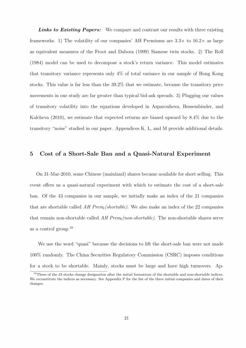
Links to Existing Papers: We compare and contrast our results with three existing

frameworks. 1) The volatility of our companies’ AH Premiums are 3.3× to 16.2× as large

as equivalent measures of the Froot and Dabora (1999) Siamese twin stocks. 2) The Roll

(1984) model can be used to decompose a stock’s return variance. This model estimates

that transitory variance represents only 4% of total variance in our sample of Hong Kong

stocks. This value is far less than the 39.2% that we estimate, because the transitory price

movements in our study are far greater than typical bid-ask spreads. 3) Plugging our values

of transitory volatility into the equations developed in Asparouhova, Bessembinder, and

Kalcheva (2010), we estimate that expected returns are biased upward by 8.4% due to the

transitory “noise” studied in our paper. Appendices K, L, and M provide additional details.

5 Cost of a Short-Sale Ban and a Quasi-Natural Experiment

On 31-Mar-2010, some Chinese (mainland) shares became available for short selling. This

event offers us a quasi-natural experiment with which to estimate the cost of a short-sale

ban. Of the 43 companies in our sample, we initially make an index of the 21 companies

that are shortable called AH Premt(shortable). We also make an index of the 22 companies

that remain non-shortable called AH Premt(non-shortable). The non-shortable shares serve

as a control group.10

We use the word “quasi” because the decisions to lift the short-sale ban were not made

100% randomly. The China Securities Regulatory Commission (CSRC) imposes conditions

for a stock to be shortable. Mainly, stocks must be large and have high turnovers. Ap-

10Three of the 43 stocks change designation after the initial formations of the shortable and non-shortable indices.We reconstitute the indices as necessary. See Appendix P for the list of the three initial companies and dates of theirchanges.

21

pendix P provides a list of CSRC conditions. It turns out that most shortable stocks are

included in one of two well-followed indices (the Shanghai 50 Index or the Shenzhen Com-

ponent Index of 40 stocks).

Appendix P provides overview statistics for the shortable and non-shortable shares. Not

surprisingly, the companies with shortable shares are larger than the companies with non-

shortable shares since size is one criterion used by the CSRC. Both share types have similar

turnovers in both the a- and h-share markets. Order imbalances are slightly more correlated

(across markets) for the non-shortable companies.

Other differences between the shortable and non-shortable companies are controlled for

by our research design. We look at changes to price behaviors around a specific event (a

difference-in-difference methodology). In addition, we look at changes to relative share price

differences (by stock pair) around the specific event. We focus on two time periods. The

“pre-period” is nine months before the ban (from Jul-2009 to Mar-2010). The “post-period”

is nine months after the ban (from Apr-2010 to Dec-2010).

Index Levels: The AH Premium of the shortable index falls from a pre-period average

of 119.0 to a post-period average of 97.7, which represents a drop of 17.9%. During the

pre-period, the shortable index had a standard deviation of 9.2 per week, which fell to 5.9

in the post-period.

The AH Premium of the non-shortable index (our control group) experienced only a

slight decline during the same periods. The pre-period average was 155.9 and the post-

period average was 145.5, which represents a drop of only 6.7%. During the pre-period, the

non-shortable index had a standard deviation of 7.4 per week, which actually rose to 8.1 in

the post-period.

22

Volatilities of Index Changes (Returns) and Transitory Prices: We use the back-

of-the envelope methodology described in Section 4.4 to decompose prices and calculate Hong

Kong transitory volatilities. As can been seen in Table V, Panel A, the h-share volatility

of the shortable group drops from 3.63% to 2.78% per week around the lifting of the ban.

The h-share volatility of AH Premt(shortable) drops too. Most importantly, the h-share

transitory volatility drops from 2.30% to 1.81% during this period.

[ Insert Table V About Here ]

Using the non-shortable shares as a control group, we see that the total volatility of these

h-share returns goes up during the same period, as does AH Premt(non-shortable). Most

importantly, the transitory volatility these h-shares goes up by 0.53%.

We conclude that lifting the short-sale ban has two effects. First, dual-listed share

price discrepancies can disappear.11 Second, decreasing frictions in one market can decrease

transitory volatility in other markets by enabling hedging mechanisms. Our results show

that lifting the short-sale ban in China (mainland) reduces transitory volatility of affected

Hong-Kong shares by 49 bp per week. No such reduction happens for the dual-listed h-shares

with the ban still in place.

6 Conclusions

This paper studies a sample of 43 large, high-profile, high-turnover companies with

dual-listed shares in China (mainland) and Hong Kong. One goal is to answer the question:

11Appendix I looks at the eight companies in our sample that have shares listed in both New York City and inHong Kong. Neither market has a short-sale ban. Dual-listed shares in New York and Hong Kong trade at parity.These findings provide additional strong support for the conclusions reached in this paper.

23

Why do the relative prices of two very similar securities exhibit large and volatile price

differences? On average, prices in China are 1.8× prices in Hong Kong. More importantly,

a given company’s price difference is very volatile.

We focus on two main frictions. The first is a short-sale ban in China. The second

is the limited risk-bearing capacity of arbitrageurs. To structure our study, we provide a

parsimonious theoretical framework that produces seven testable implications. We are able

to make predictions about the level and dynamics of a company’s AH Premium, which is

the ratio of its China a-share price to its Hong Kong h-share price.

Many of this paper’s empirical results come from estimating a state-space model (SSM).

The statistical model assumes that a stock’s observable price is composed of two unobservable

components. For dual-listed shares, we assume a given company has a single efficient price

at each point in time and two transitory prices. Using order flows from each market, we

have a new method of identifying a company’s unobservable components. In addition, our

research design allows us to carry out two back-of-the-envelope calculations that confirm the

SSM estimates. Finally, an ARMA estimation also confirms our findings. Our paper offers

a number of results:

• A one standard-deviation shock to order flow in China (mainland) leads to a 150 bp

change in transitory prices in China.

• A one standard-deviation shock to order flow in Hong Kong leads to a 112 bp change

in transitory prices in Hong Kong.

• Cross-sectionally, companies with fundamental volatilities one standard deviation above

the mean have average AH Premiums of 274.6, while companies one standard deviation

below the mean have average AH Premiums of 83.34.

24

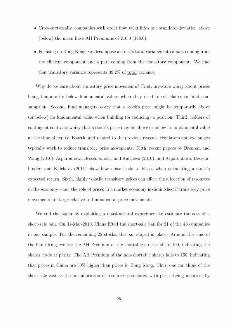
• Cross-sectionally, companies with order flow volatilities one standard deviation above

(below) the mean have AH Premiums of 210.0 (148.0).

• Focusing on Hong Kong, we decompose a stock’s total variance into a part coming from

the efficient component and a part coming from the transitory component. We find

that transitory variance represents 39.2% of total variance.

Why do we care about transitory price movements? First, investors worry about prices

being temporarily below fundamental values when they need to sell shares to fund con-

sumption. Second, fund managers worry that a stock’s price might be temporarily above

(or below) its fundamental value when building (or reducing) a position. Third, holders of

contingent contracts worry that a stock’s price may be above or below its fundamental value

at the time of expiry. Fourth, and related to the previous reasons, regulators and exchanges

typically work to reduce transitory price movements. Fifth, recent papers by Brennan and

Wang (2010), Asparouhova, Bessembinder, and Kalcheva (2010), and Asparouhova, Bessem-

binder, and Kalcheva (2011) show how noise leads to biases when calculating a stock’s

expected return. Sixth, highly volatile transitory prices can affect the allocation of resources

in the economy—i.e., the role of prices in a market economy is diminished if transitory price

movements are large relative to fundamental price movements.

We end the paper by exploiting a quasi-natural experiment to estimate the cost of a

short-sale ban. On 31-Mar-2010, China lifted the short-sale ban for 21 of the 43 companies

in our sample. For the remaining 22 stocks, the ban stayed in place. Around the time of

the ban lifting, we see the AH Premium of the shortable stocks fall to 100, indicating the

shares trade at parity. The AH Premium of the non-shortable shares falls to 150, indicating

that prices in China are 50% higher than prices in Hong Kong. Thus, one can think of the

short-sale cost as the mis-allocation of resources associated with prices being incorrect by

25

50%.

Alternatively, we show that lifting of the short-sale constraint in China reduces the

transitory volatility of the associated Hong Kong shares by 49 bp. There is no reduction in

transitory volatility for the shares that remain non-shortable (our control group). In fact, the

transitory volatility of the control group actually goes up. The results show that a friction

in an emerging stock market can affect prices in a developed market by restricting access to

hedging instruments.

There are a number of research agendas that follow naturally from our paper:

• One could incorporate brokerage account data into our state-space estimation. With

such data, one might be able to construct order imbalance measures for relatively naive

individuals and for relatively sophisticated institutions. Estimates that incorporate

these order imbalances may lead to additional insights into the movements of a stock’s

transitory and fundamental components.

• Economists may want to investigate whether large price impacts associated with order

imbalances indicate a need to attract more capital into the market-making (arbitrage)

sector of the economy. One might be able to show a decrease in transitory price

movements after an increase in market-making capital.

• There may be a link between our findings and investment industry practices. Future

work could ask: How do fund managers build (or reduce) a position in markets with

high levels of transitory price movements? Since a stock’s transitory component (si,t)

is not observable, one never knows if a price is temporarily high or low. Waiting incurs

opportunity costs. If investors are risk-averse, it may make sense to dollar-cost average

over a given period of time (presumably related to the half-life of the transitory shocks).

26

• Finally, it would be interesting to link the degree of transitory price movements doc-

umented in this paper to welfare losses stemming from the inefficient allocation of

resources in the economy. To accomplish this goal, one needs a general equilibrium

model that allows prices to have non-zero transitory components.

The above list of projects is potentially interesting to finance professionals, economists,

and policy makers. Each project builds on the fundamental result of our paper—there is

substantial “noise” in prices. This noise is relevant for large stocks in developed markets.

The noise is not short lived and may affect prices for weeks and even months.

27

References

Asparouhova, E., H. Bessembinder, and I. Kalcheva. 2010. “Liquidity biases in asset pricing

tests.” Journal of Financial Economics 96:215–237.

. 2011. “Noisy prices and inference regarding returns.” Forthcoming Journal of

Finance.

Baruch, S., G.A. Karolyi, and M.L. Lemmon. 2007. “Multimarket trading and liquidity:

Theory and evidence.” Journal of Finance 62(5):2169–2200.

Brennan, M.J., and A.W. Wang. 2010. “The Mispricing Return Premium.” 23(9):3437–

3468.

Chan, K., A. Hameed, and S.T. Lau. 2003. “What if trading locations is different from

business location? Evidence from the Jardine Group.” Journal of Finance 58(3):1221–

1246.

Chan, K., H.W. Kot, and Z. Yang. 2010. “Effects of short-sale constraints on stock prices

and trading activity: Evidence from Hong Kong and mainland China.” Working Paper.

Chan, K., A.J. Menkveld, and Z. Yang. 2007. “The informativeness of domestic and foreign

investors’ stock trades: Evidence from the perfectly segmented Chinese market.” Journal

of Financial Markets 10:391–415.

. 2008. “Information asymmetry and asset prices: Evidence from the China foreign

share discount.” Journal of Finance 63(1):159–196.

DeJong, A., L. Rosenthal, and M.A. Van Dijk. 2009. “The risk and return of arbitrage in

dual-listed companies.” Review of Finance 13:495–520.

Froot, K.A., and E.M. Dabora. 1999. “How are stocks prices affected by the location of

trade?” Journal of Financial Economics 53:189–216.

28

Froot, K.A., and Tarun Ramadorai. 2008. “Institutional portfolio flows and international

investments.” Review of Financial Studies 21(2):937–971.

Gagnon, L., and G.A. Karolyi. 2010a. “Do international cross-listings still matter?” Evi-

dence of Financial Globalization and Crises.

. 2010b. “Multi-market trading and arbitrage.” Journal of Financial Economics

97:53–80.

Grossman, S.J., and M.H. Miller. 1988. “Liquidity and market structure.” Journal of

Finance 43(3):617–637.

Halling, M., P.C. Moulton, and M. Panayides. 2011. “Volume dynamics and multimarket

trading.” Working Paper.

Hasbrouck, J. 1993. “Assessing the quality of a security market: A new approach to

transaction cost measurement.” Review of Financial Studies 6(1):191–212.

Hendershott, T., S.X. Li, A.J. Menkveld, and M.S. Seasholes. 2010. “Risk sharing, costly

participation, and monthly returns.” Working Paper.

Hendershott, T., and A.J. Menkveld. 2010. “Price pressures.” Working Paper.

Karolyi, G.A. 2010. “Corporate governance, agency problems and international cross-

listings: A defense of the bonding hypothesis.” Working Paper.

Koopman, S.J., N. Shephard, and J.A. Doornik. 1999. “Statistical algorithms for models

in state space using ssfpack 2.2.” Econometrics Journal 2:113–166.

Lauterbach, B., and A. Wohl. 2001. “A note on price noises and their correction process:

Evidence from two equal-payooff government bonds.” Journal of Banking & Finance

25:597–612.

Mei, J.P., J.A. Scheinkman, and W. Xiong. 2009. “Speculative trading and stock prices:

29

Evidence from Chinese A-B share premia.” Annals of Economics and Finance 10(2):225–

255.

Menkveld, A.J., S.J. Koopman, and A. Lucas. 2007. “Modeling around-the-clock price dis-

covery for cross-listed stocks using state space models.” Journal of Business & Economic

Statistics 25:213–225.

Roll, R. 1984. “A simple implicit measure of the effective bid-ask spread in an efficient

market.” Journal of Finance 39:1127–1140.

Rosenthal, L., and C. Young. 1990. “The seemingly anomalous price behavior of Royal

Dutch Shell and Unilever N.V. PLC.” Journal of Financial Economics 26:123–141.

Scruggs, J.T. 2007. “Noise trader risk: Evidence from Siamese twins.” Journal of Financial

Markets 10:76–105.

Seasholes, M.S., and C. Liu. 2011. “Trading imbalances and the law of one price.” Economic

Letters 112:132–134.

30

Table I — Panel A

Overview of Companies in Our Sample

The table shows the 43 companies in our data sample. A-shares trade in China (mainland). H-shares trade in Hong

Kong. Market capitalizations are in millions of US dollars. Industries are based on Global Industry Classification

Standard (GICS) codes. The final column shows the number of weeks a company is in our sample.

A H Tot Mkt Cap HK Mkt Cap Industry # of Wks

Name Ticker Ticker (US$ mil) (US$ mil) (GICS Codes) of Data

Air China 601111 0753 9,537 2,046 Airlines 140

Anhui Conch 600585 0914 10,644 2,663 Construction Mat. 173

Anhui Expressway 600012 0995 1,106 244 Transport Infra. 165

Bank of China 601988 3988 119,676 27,759 Comm. Banks 147

Bankcomm 601328 3328 44,041 18,183 Comm. Banks 102

Beijing N Star 601588 0588 1,918 150 Real Estate 132

CCB 601939 0939 133,111 127,272 Comm. Banks 82

CHALCO 601600 2600 17,320 2,926 Metals & Mining 104

China Coal 601898 1898 17,451 3,460 Oil, Gas & Fuels 60

China COSCO 601919 1919 15,787 2,068 Marine 96

China East Air 600115 0670 2,531 265 Airlines 60

China Life 601628 2628 97,611 25,587 Insurance 120

China Oilfield 601808 2883 7,712 1,166 Energy Equip. 82

China Rail Cons 601186 1186 17,257 2,877 Constr & Engin. 34

China Railway 601390 0390 17,153 2,861 Constr & Engin. 60

China Shenhua 601088 1088 68,952 9,209 Oil, Gas & Fuels 78

China Ship Dev 600026 1138 5,333 1,440 Marine 173

China South Air 600029 1055 4,249 418 Airlines 86

Chongqing Iron 601005 1053 987 159 Metals & Mining 86

CITIC Bank 601998 0998 24,897 5,633 Comm. Banks 86

CM Bank 600036 3968 32,930 4,850 Comm. Banks 135

CSCL 601866 2866 5,748 881 Marine 69

CSR 601766 1766 7,312 930 Machinery 8

Datang Power 601991 0991 10,441 1,591 Indep Power 123

Dongfang Elec 600875 1072 4,586 418 Elec. Equip. 173

Guangshen Rail 601333 0525 4,643 621 Road & Rail 122

Guangzhou Pharm 600332 0874 786 84 Pharmaceut 173

Guangzhou Ship 600685 0317 1,300 199 Machinery 86

Huadian Power 600027 1071 3,652 379 Indep Power 173

Huaneng Power 600011 0902 12,162 2,093 Indep Power 173

ICBC 601398 1398 197,229 46,189 Comm. Banks 130

Jiangsu Express 600377 0177 4,147 856 Transportation 173

Jiangxi Copper 600362 0358 7,233 1,565 Metals & Mining 173

Maanshan Iron 600808 0323 4,109 666 Metals & Mining 173

PetroChina 601857 0857 293,150 18,104 Oil, Gas & Fuels 73

Ping An 601318 2318 42,977 15,467 Insurance 112

SH Electric 601727 2727 12,568 994 Elec. Equip. 17

ShenzhenExpress 600548 0548 1,391 283 Transportation 173

Sinopec Corp 600028 0386 111,978 12,558 Oil, Gas & Fuels 173

Tianjin Capital 600874 1065 1,040 64 Comm Svcs 173

Tsingtao Brew 600600 0168 3,809 1,521 Beverages 173

Yanzhou Coal 600188 1171 7,980 1,769 Oil, Gas & Fuels 173

Zijin Mining 601899 2899 16,667 3,122 Metals & Mining 52

Average 32,677 8,176 118

Median 9,537 1,591 122

31

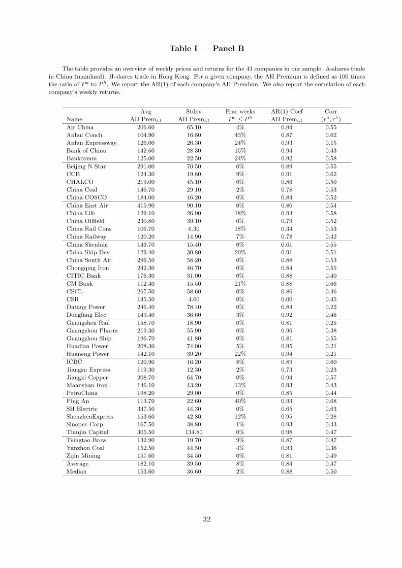
Table I — Panel B

The table provides an overview of weekly prices and returns for the 43 companies in our sample. A-shares trade

in China (mainland). H-shares trade in Hong Kong. For a given company, the AH Premium is defined as 100 times

the ratio of P a to Ph. We report the AR(1) of each company’s AH Premium. We also report the correlation of each

company’s weekly returns.

Avg Stdev Frac weeks AR(1) Coef Corr

Name AH Premi,t AH Premi,t P a ≤ Ph AH Premi,t (ra, rh)

Air China 206.60 65.10 4% 0.94 0.55

Anhui Conch 104.90 16.80 43% 0.87 0.62

Anhui Expressway 126.00 26.30 24% 0.93 0.15

Bank of China 142.60 28.30 15% 0.94 0.43

Bankcomm 125.00 22.50 24% 0.92 0.58

Beijing N Star 291.00 70.50 0% 0.89 0.55

CCB 124.30 19.80 9% 0.91 0.62

CHALCO 219.00 45.10 0% 0.86 0.50

China Coal 146.70 29.10 2% 0.78 0.53

China COSCO 184.00 46.20 0% 0.84 0.52

China East Air 415.90 90.10 0% 0.86 0.54

China Life 129.10 26.90 18% 0.94 0.58

China Oilfield 230.80 39.10 0% 0.79 0.52

China Rail Cons 106.70 6.30 18% 0.34 0.53

China Railway 120.20 14.90 7% 0.78 0.42

China Shenhua 143.70 15.40 0% 0.61 0.55

China Ship Dev 129.40 30.80 20% 0.91 0.51

China South Air 296.50 58.20 0% 0.88 0.53

Chongqing Iron 242.30 46.70 0% 0.84 0.55

CITIC Bank 176.30 31.00 0% 0.88 0.40

CM Bank 112.40 15.50 21% 0.88 0.66

CSCL 267.50 58.60 0% 0.86 0.46

CSR 145.50 4.60 0% 0.00 0.45

Datang Power 246.40 78.40 0% 0.84 0.22

Dongfang Elec 149.40 36.60 3% 0.92 0.46

Guangshen Rail 158.70 18.90 0% 0.81 0.25

Guangzhou Pharm 219.30 55.90 0% 0.96 0.38

Guangzhou Ship 196.70 41.80 0% 0.81 0.55

Huadian Power 208.30 74.00 5% 0.95 0.21

Huaneng Power 142.10 39.20 22% 0.94 0.21

ICBC 120.90 16.20 8% 0.89 0.60

Jiangsu Express 119.30 12.30 2% 0.73 0.23

Jiangxi Copper 208.70 64.70 0% 0.94 0.57

Maanshan Iron 146.10 43.20 13% 0.93 0.43

PetroChina 198.20 29.00 0% 0.85 0.44

Ping An 113.70 22.60 40% 0.93 0.68

SH Electric 347.50 44.30 0% 0.65 0.63

ShenzhenExpress 153.60 42.80 12% 0.95 0.28

Sinopec Corp 167.50 38.80 1% 0.93 0.43

Tianjin Capital 305.50 134.80 0% 0.98 0.47

Tsingtao Brew 132.90 19.70 9% 0.87 0.47

Yanzhou Coal 152.50 44.50 4% 0.93 0.36

Zijin Mining 157.60 34.50 0% 0.81 0.49

Average 182.10 39.50 8% 0.84 0.47

Median 153.60 36.60 2% 0.88 0.50

32

Table I — Panel C

The table provides an overview of weekly trading variables for the 43 companies in our sample. A-shares trade

in China (mainland). H-shares trade in Hong Kong. Columns 2 and 3 report free floats as percentages of shares

listed. Columns 4 and 5 report average weekly turnover, by company, as percentages of shares available to trade (free

floats). We also report each company’s correlation of weekly order imbalances.

Free Float Free Float Avg Avg Corr

Name Mkt a Mkt h Turn(a) Turn(h) (OIBa, OIBh)

Air China 0.16 0.54 0.17 0.07 0.20

Anhui Conch 0.26 1.00 0.07 0.04 0.12

Anhui Expressway 0.33 1.00 0.10 0.02 0.09

Bank of China 0.03 0.39 0.11 0.07 0.07

Bankcomm 0.25 0.62 0.10 0.03 -0.09

Beijing N Star 0.43 1.00 0.24 0.05 0.11

CCB 0.92 0.20 0.07 0.04 -0.25

CHALCO 0.21 1.00 0.11 0.07 0.12

China Coal 0.18 0.98 0.13 0.05 -0.11

China COSCO 0.20 0.96 0.15 0.10 0.09

China East Air 0.15 1.00 0.13 0.06 -0.11

China Life 0.05 1.00 0.12 0.07 0.07

China Oilfield 0.19 1.00 0.09 0.04 -0.32

China Rail Cons 0.25 0.85 0.11 0.05 -0.08

China Railway 0.26 0.91 0.11 0.05 0.02

China Shenhua 0.11 1.00 0.07 0.05 -0.20

China Ship Dev 0.26 1.00 0.14 0.04 0.11

China South Air 0.35 0.95 0.15 0.07 -0.10

Chongqing Iron 0.30 1.00 0.12 0.05 0.30

CITIC Bank 0.07 0.41 0.07 0.05 0.33

CM Bank 0.46 1.00 0.06 0.07 0.02

CSCL 0.27 0.96 0.09 0.10 0.10

CSR 0.35 0.90 0.21 0.06 -0.06

Datang Power 0.30 1.00 0.15 0.06 -0.07

Dongfang Elec 0.29 1.00 0.11 0.04 -0.09

Guangshen Rail 0.39 1.00 0.14 0.03 0.07

Guangzhou Pharm 0.23 1.00 0.15 0.03 -0.04

Guangzhou Ship 0.50 1.00 0.15 0.06 0.09

Huadian Power 0.21 1.00 0.11 0.05 0.06

Huaneng Power 0.21 1.00 0.08 0.04 -0.03

ICBC 0.04 0.48 0.12 0.06 -0.22

Jiangsu Express 0.09 1.00 0.11 0.03 -0.10

Jiangxi Copper 0.20 1.00 0.21 0.11 0.04

Maanshan Iron 0.22 1.00 0.17 0.10 0.15

PetroChina 0.02 1.00 0.06 0.04 -0.23

Ping An 0.35 0.54 0.09 0.06 0.05

SH Electric 0.07 1.00 0.35 0.07 0.09

ShenzhenExpress 0.20 1.00 0.12 0.02 -0.03

Sinopec Corp 0.06 1.00 0.10 0.05 0.10

Tianjin Capital 0.25 1.00 0.24 0.05 0.04

Tsingtao Brew 0.40 0.50 0.07 0.03 -0.07

Yanzhou Coal 0.15 1.00 0.16 0.07 0.02

Zijin Mining 0.11 1.00 0.34 0.05 0.28

Average 0.24 0.89 0.13 0.05 0.01

Median 0.22 1.00 0.12 0.05 0.04

33

Table II

Parameter Estimates

This table shows parameter estimates for the state-space model shown in Equation (2) and directly

below. We estimate the equations on a stock-by-stock basis and report average coefficients. There is sufficient

data to estimate parameters for 41 of the 43 stocks in our sample.

pai,t = mi,t + sai,t + ci

phi,t = mi,t + shi,t

mi,t = mi,t−1 + δi,t + wi,t

wi,t = κaOIBai,t + κhOIBhi,t + ui,t

sai,t = φasai,t−1 + γaOIBai,t + εai,t

shi,t = φhshi,t−1 + γhOIBhi,t + εhi,t

κa κh σu

Param 0.0022 -0.0002 0.0274

Stderr (0.0005) (0.0004) (0.0021)

φa φh γa γh σε(a) σε(h)

Param 0.8524 0.8430 0.0052 0.0038 0.0582 0.0585

Stderr (0.0067) (0.0124) (0.0006) (0.0006) (0.0024) (0.0023)

34

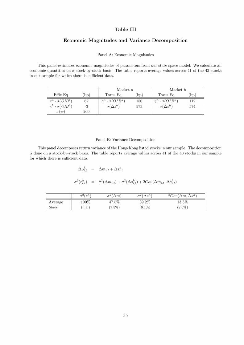
Table III

Economic Magnitudes and Variance Decomposition

Panel A: Economic Magnitudes

This panel estimates economic magnitudes of parameters from our state-space model. We calculate all

economic quantities on a stock-by-stock basis. The table reports average values across 41 of the 43 stocks

in our sample for which there is sufficient data.

Market a Market h

Effic Eq (bp) Trans Eq (bp) Trans Eq (bp)

κa · σ(OIBa) 62 γa · σ(OIBa) 150 γh · σ(OIBh) 112

κh · σ(OIBh) -3 σ(∆sa) 573 σ(∆sh) 574

σ(w) 200

Panel B: Variance Decomposition

This panel decomposes return variance of the Hong-Kong listed stocks in our sample. The decomposition

is done on a stock-by-stock basis. The table reports average values across 41 of the 43 stocks in our sample

for which there is sufficient data.

∆phi,t = ∆mi,t + ∆shi,t

σ2(rhi,t) = σ2(∆mi,t) + σ2(∆shi,t) + 2Cov(∆mi,t,∆shi,t)

σ2(rh) σ2(∆m) σ2(∆sh) 2Cov(∆m,∆sh)

Average 100% 47.5% 39.2% 13.3%

Stderr (n.a.) (7.5%) (6.1%) (2.0%)

35

Table IV

Cross-Sectional Implications for AH Prem i,t

Panel A: Fundamental Volatility and AH Premi,t

This panel shows cross-sectional regression results of AH Premi on fundamental volatility. In Reg1, the

LHS variable is a company’s average AH Premi,t over our sample period. In Reg2, we include the natural

log of a company’s market capitalization as a control variable. In Reg3, the LHS variable is a company’s

final value of AH Premi,t. Each company’s σi(w) comes from our state-space model.

AH Premi = β0 + β1σi(w) + β2ln(MktCapi) + εi

Coef Reg1 Reg2 Reg3

β0 118.60 266.11 137.15

(t-stat) (5.30) (4.01) (4.57)

β1 0.30 0.23 0.32

(t-stat) (2.98) (2.31) (2.36)

β2 -14.42

(t-stat) (-2.34)

Obs 41 41 41

LHS Variable Average Average Final

AH Premi,t AH Premi,t AH Premi,t

36

Table IV — Panel B

Panel B: Trading Volatility and AH Premi,t

This panel shows cross-sectional regression results of AH Premi on trading volatility. In Reg1 - Reg4

we use RHS variables related to order imbalances in market a. In Reg5 - Reg8 we use RHS variables related

to order imbalances in market h. In Reg9 we use trading variables from both markets. The RHS variables

tested are either 1,000·γai , 1,000·γhi , γai ·σ(OIBa), or γhi ·σ(OIBh), where γai and γhi are from our state-space

model.

AH Premi = β0 + βa1 (1000 · γai ) + βh1(1000 · γhi

)+ β2ln(MktCapi) + εi

Coef Reg1 Reg2 Reg3 Reg4

β0 133.82 117.43 274.24 217.14

(t-stat) (8.02) (7.93) (4.46) (3.67)

βa1 8.68 0.41 6.95 0.35

(t-stat) (3.27) (5.01) (2.66) (4.09)

βh1(t-stat)

β2 -14.19 -9.84

(t-stat) (-2.36) (-1.74)

Obs 41 41 41 41

Main RHS

Variable 1,000·γai γai · σ(OIBa) 1,000·γai γai · σ(OIBa)

Coef Reg5 Reg6 Reg7 Reg8 Reg9

β0 158.73 156.69 313.85 305.82 124.12

(t-stat) (11.43) (11.49) (4.95) (4.80) (7.12)

βa1 7.75

(t-stat) (2.91)

βh1 5.39 0.20 3.55 0.13 3.88

(t-stat) (2.11) (2.37) (1.41) (1.61) (1.61)

β2 -16.00 -15.33

(t-stat) (-2.50) (-2.39)

Obs 41 41 41 41 41

Main RHS 1,000·γhi γhi · σ(OIBh) 1,000·γhi γhi · σ(OIBh) 1,000·γaiVariable(s) and

1,000·γhi

37

Table V

Quasi Natural Experiment

Panel A: Index of Shortable Shares

This panel shows results related to an index of shortable share pairs. The index is initially formed

using the same methodology as the AH Premium Index but only considers the 21 companies for which the

short-sale ban was lifted in China (mainland). We consider two periods: nine months before the short-sale

ban is lifted (Jul-2009 to Mar-2010) and nine months after (Apr-2010 to Dec-2010). The column with rh

shows the standard deviation of the Hong Kong shares (only). The column with rah shows the standard

deviation of log changes to the AH Premium Index. The column with sh shows the transitory volatility of

Hong Kong shares (only). Transitory volatility is estimated using the back-of-the-envelope method described

in Section 4.4.

Start End Stdev(rh) Stdev(rah) Stdev(sh)

01-Jul-2009 31-Mar-2010 0.0363 0.0325 0.0230

01-Apr-2010 31-Dec-2010 0.0278 0.0256 0.0181

Diff -0.0049

Panel B: Index of Non-Shortable Shares

This panel mirrors the panel above, but shows results related an index of non-shortable share pairs.

The index is initially formed using the same methodology as the AH Premium Index but only considers the

22 companies for which the short-sale ban was not lifted in China (mainland).

Start End Stdev(rh) Stdev(rah) Stdev(sh)

01-Jul-2009 31-Mar-2010 0.0416 0.0351 0.0248

01-Apr-2010 31-Dec-2010 0.0425 0.0426 0.0301

Diff 0.0053

38

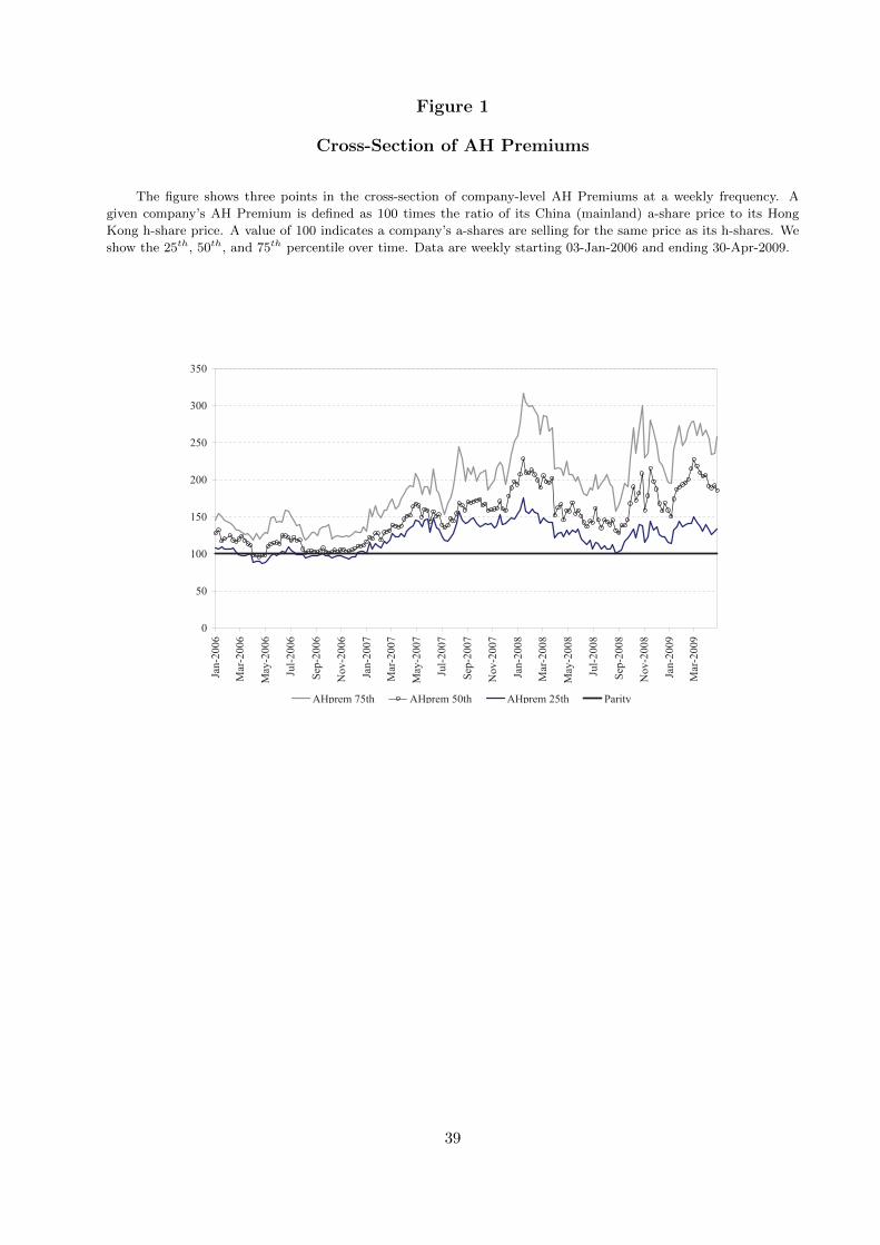
Figure 1

Cross-Section of AH Premiums

The figure shows three points in the cross-section of company-level AH Premiums at a weekly frequency. A

given company’s AH Premium is defined as 100 times the ratio of its China (mainland) a-share price to its Hong

Kong h-share price. A value of 100 indicates a company’s a-shares are selling for the same price as its h-shares. We

show the 25th, 50th, and 75th percentile over time. Data are weekly starting 03-Jan-2006 and ending 30-Apr-2009.

0

50

100

150

200

250

300

350

Jan

-20

06

Mar

-20

06

May

-20

06

Jul-

20

06

Sep

-20

06

No

v-2

00

6

Jan

-20

07

Mar

-20

07

May

-20

07

Jul-

20

07

Sep

-20

07

No

v-2

00

7

Jan

-20

08

Mar

-20

08

May

-20

08

Jul-

20

08

Sep

-20

08

No

v-2

00

8

Jan

-20

09

Mar

-20

09

AHprem 75th AHprem 50th AHprem 25th Parity

39

Figure 2

AH Premiums for Three Companies

The figure shows the time-series of AH Premiums for three companies at a weekly frequency. A given company’s

AH Premium is defined as 100 times the ratio of its China (mainland) a-share price to its Hong Kong h-share price.

A value of 100 indicates a company’s a-shares are selling for the same price as its h-shares. The first company is

Jiangxi Copper. The second company is Shenzhen Expressway. The third company is China Shipping. Data are

weekly starting 03-Jan-2006 and ending 30-Apr-2009.

0

50

100

150

200

250

300

350

400

450

Jan

-20

06

Mar

-20

06

May

-20

06

Jul-

20

06

Sep

-20

06

No

v-2

00

6

Jan

-20

07

Mar

-20

07

May

-20

07

Jul-

20

07

Sep

-20

07

No

v-2

00

7

Jan

-20

08

Mar

-20

08

May

-20

08

Jul-

20

08

Sep

-20

08

No

v-2

00

8

Jan

-20

09

Mar

-20

09

Jiangxi Copper Shenzhen Expressway China Ship Parity

40