Dsp manual print

1. TO STUDY THE ARCHITECTURE OF DSP CHIPS -TMS 320C SX/6X INSTRUCTIONS.

The C6711™ DSK builds on TI's industry-leading line of low cost, easy-to-use DSP Starter

Kit (DSK) development boards. The high-performance board features the

TMS320C6711 floating-point DSP. Capable of performing 900 million floating-point

operations per second (MFLOPS), the C6711 DSP makes the C6711 DSK the most

powerful DSK development board on the market.

The DSK is a parallel port interfaced platform that allows TI, its customers, and thirdparties,

to efficiently develop and test applications for the C6711. The DSK consists of a C6711-

based printed circuit board that will serve as a hardware reference design for TI’s

customers’ products. With extensive host PC and target DSP software support,

including bundled TI tools, the DSK provides ease-of-use and capabilities that are

attractive to DSP engineers.

TMS320C6711 DSK Block Diagram

The basic function block diagram and interfaces of the C6711 DSK are displayed

below.

Many of the parts of the block diagram are linked to specific topics.

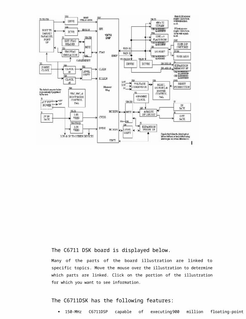
The C6711 DSK board is displayed below.

Many of the parts of the board illustration are linked to specific topics. Move the mouse

over the illustration to determine which parts are linked. Click on the portion of the illustration

for which you want to see information.

The C6711DSK has the following features:

150-MHz C6711DSP capable of executing 900 million floating-point

operations per second (MFLOPS)

Dual clock support; CPU at 150MHz and external memory interface (EMIF) at

100MHz

Parallel port controller (PPC) interface to standard parallel port on a host PC

(EEP or bi-directional SPP support)

16M Bytes of 100 MHz synchronous dynamic random access memory

(SDRAM)

128K Bytes of flash programmable and erasable read only memory (ROM)

8-bit memory-mapped I/O port

Embedded JTAG emulation via the parallel port and external XDS510 support

Host port interface (HPI) access to all DSP memory via the parallel port

16-bit audio codec

Onboard switching voltage regulators for 1.8 volts direct current (VDC) and

3.3 VDC

The C6711 DSK has approximate dimensions of 5.02 inches wide, 8.08 inches long

and 0.7 inches high. The C6711 DSK is intended for desktop operation while

connected to the parallel port of your PC or using an XDS510 emulator. The DSK

requires that the external power supply be connected in either mode of operation (an

external power supply and a parallel cable are provided in the kit).

The C6711 DSK has a TMS320C6711 DSP onboard that allows full-speed

verification of code with Code Composer Studio. The C6711 DSK provides:

a parallel peripheral interface

SDRAM and ROM

a 16-bit analog interface circuit (AIC)

an I/O port

embedded JTAG emulation support

Connectors on the C6711 DSK provide DSP external memory interface (EMIF) and

peripheral signals that enable its functionality to be expanded with custom or third party

daughter boards.

The DSK provides a C6711 hardware reference design that can assist you in the

development of your own C6711-based products. In addition to providing a reference for

interfacing the DSP to various types of memories and peripherals, the design also

addresses power, clock, JTAG, and parallel peripheral interfaces.

Top Side of the Board:

Bottom Side of the Board:

TMS320C6711 DSP Features:

VelociTI advanced very long instruction word (VLIW) architecture

Load-store architecture

Instruction packaging for reduced code size

100% conditional instructions for faster execution

Intuitive, reduced instruction set computing with RISC-like instruction set

CPU

Eight highly independent functional units (including six ALUs and twomultipliers)

32 32-bit general-purpose registers

900 million floating-point operations per second (MIPS)

6.7-ns cycle time

Up to eight 32-bit instructions per cycle

Byte-addressable (8-, 16-, 32-bit data)

32-bit address range

8-bit overflow protection

Little- and big-endian support

Saturation

Normalization

Bit-field instructions (extract, set, clear)

Bit-counting

Memory/peripherals

L1/L2 memory architecture:

32K-bit (4-K byte) L1P program cache (direct mapped)

32K-bit (4K-byte) L1D data cache (2-way set-associative)

512K-bit (64K byte) L2 unified map RAM/cache (flexible data/program allocation) 32-bit

external memory interface (EMIF):

Glue less interface to synchronous memories: SDRAM and SBSRAM Glue

less interface to asynchronous memories: SDRAM and EPROM Enhanced

direct-memory-access (EDMA) controller

16-bit host-port interface (HPI) (access to entire memory map) Two

multi-channel buffered serial ports (McBSPs)

Two 32-bit general-purpose timers

Flexible phase-locked-loop (PLL) clock generator

Miscellaneous

IEEE-1149.1 (JTAG) boundary-scan-compatible for emulation and test support 256-

lead ball grid array (BGA) package (GFN suffix)

0.18-mm/5-level metal process with CMOS technology

3.3-V I/Os, 1/8-V internal

C67x (Specific) Floating-Point Instructions:

Alphabetical Listing of 'C67x (Specific) Floating-Point Instructions A - F

G - L M - R S - Z

ABSDP INTDP MPYDP SPDP

ABSSP INTDPU MPYI SPINT

ADDAD INTSP MPYID SPTRUNC

ADDDP INTSPU MPYSP SUBDP

ADDSP LDDW RCPDP SUBSP

CMPEQDP RCPSP

CMPEQSP RSQRDP

CMPGTDP RSQRSP

CMPGTSP

CMPLTDP

CMPLTSP

DPINT

DPSP

DPTRUNC

2. TO VERIFY LINEAR CONVOLUTION

Aim: To compute the linear convolution of two discrete sequences.

Theory: Consider two finite duration sequences x (n) and h (n), the duration of x

(n) is n1 samples in the interval 0 n (n1 1). The duration of h (n) is n2 samples;

that is h (n) is non - zero only in the interval 0 n (n2 1) . The linear or a periodicconvolution of x (n) and h (n) yields the sequence y (n) defined as,

n

Y (n) = ∑h(m)x(n m)m0

Clearly, y (n) is a finite duration sequence of duration (n1+n2 -1) samples. The convolution sum of two sequences can be found by using following steps

Step1: Choose an initial value of n, the starting time for evaluating the output sequence y (n). If x (n) starts at n=n1 and h (n) starts at n= n2 then n = n1+ n2-1 is a good choice.

Step2: Express both sequences in terms of the index m.

Step3: Fold h (m) about m=0 to obtain h (-m) and shift by n to the right if n is positive and left if n is negative to obtain h (n-m).

Step4: Multiply two sequences x (n-m) and h (m) element by element and sum the products to get y (n).

Step5: Increment the index n, shift the sequence x (n-m) to right by one sample and repeat step4.

Step6: Repeat step5 until the sum of products is zero for all remaining values of n.

Program:

%Linear convolution of two sequences

a=input('enter the input sequence1=');

b=input('enter the input sequence2=');

n1=length (a)

n2=length (b)

x=0:1:n1-1;

Subplot (2, 2, 1), stem(x, a); title

('INPUT SEQUENCE1'); xlabel

('---->n');

ylabel ('---->a (n)');

y=0:1:n2-1;

subplot (2, 2, 2), stem(y, b); title

('INPUT SEQUENCE2'); xlabel

('---->n');

ylabel('---->b(n)');

c=conv (a, b)

n3=0:1:n1+n2-2;

subplot (2, 1, 2), stem (n3, c);

title ('CONVOLUTION OF TWO SEQUENCES');

xlabel ('---->n');

ylabel ('---->c (n)');

Output:

Enter the input sequence1=


C=



n1 =

n2 =

c =

Result:

Inference: The length of the Linear convolved sequence is n1+n2-1 where n1and n2

are lengths of sequences.

VIVA Questions

1. What do you understand by Linear Convolution.

2. What are the properties of convolution.

3. TO VERIFY CIRCULAR CONVOLUTION

Aim: To compute the circular convolution of two discrete sequences.

Theory: Two real N-periodic sequences x(n) and h(n) and their circular or periodic

convolution sequence y(n) is also an N- periodic and given by,

N

y(n) 1∑h(m)x((n m))N , for n=0 to N-1.m0

Circular convolution is some thing different from ordinary linear convolution

operation, as this involves the index ((n-m))N, which stands for a ‘modula-N’

operation. Basically both type of convolution involve same six steps. But the

difference between the two types of convolution is that in circular convolution the

folding and shifting (rotating) operations are performed in a circular fassion by

computing the index of one of the sequences with ‘modulo-N’ operation. Either one of the

two sequences may be folded and rotated without changing the result of circular

convolution. That is,

N

y(n) 1∑x(m)h((nm))N , for n=0 to (N-1).m0

If x (n) contain L no of samples and h (n) has M no of samples and that L > M, then

perform circular convolution between the two using N=max (L,M), by adding (L-M) no

of zero samples to the sequence h (n), so that both sequences are periodic with

number.

Two sequences x (n) and h (n), the circular convolution of these two sequences

can be found by using the following steps.

1. Graph N samples of h (n) as equally spaced points around an outer circle in counterclockwise direction.

2. Start at the same point as h (n) graph N samples of x (n) as equally spaced points around an inner circle in clock wise direction.

3. Multiply corresponding samples on the two circles and sum the products to produce output.

4. Rotate the inner circle one sample at a time in counter clock wise direction and go to step 3 to obtain the next value of output.

5. Repeat step No.4 until the inner circle first sample lines up with first sample of the exterior circle once again.

Program:

%circular convolution

a=input('enter the input sequence1=');

b=input('enter the input sequence2=');

n1=length (a)

n2=length (b)

n3=n1-n2

N=max (n1, n2);

if (n3>0)

b= [b, zeros (1, n1-n2)]

n2=length (b);

else

a= [a, zeros (1, N-n1)]

n1=length (a);

end;

k=max (n1, n2);

a=a';

b=b';

c=b;

for i=1: k-1

b=circshift (b, 1);

c=[c, b];

end;

disp(c);

z=c*a;

disp ('z=')

disp (z)

subplot (2, 2, 1);

stem (a,'filled');

title ('INPUT SEQUENCE1');

xlabel ('---->n');

ylabel ('---->Amplitude')

subplot (2, 2, 2);

stem (b,'filled');

title ('INPUT SEQUENCE2'); xlabel ('---->n');

ylabel ('---->Amplitude');

subplot (2, 1, 2);

stem (z,'filled');

title ('CONVOLUTION OF TWO SEQUENCES');

xlabel ('---->n');


Output:



n1 =

n2 =

n3 =

b =

z=

Result:

Inference: The length of the circularly convolved sequence is max (n1, n2) where n1

and n2 are the lengths of given sequences.

Questions & Answers

1. Define circular convolution?

2. What do you understand by periodic convolution?

4. DESIGN FIR FILTER (LP/HP) USING WINDOWING TECHNIQUE

a) USING RECTANGULAR WINDOW

Aim: To design FIR high pass filter using rectangular window.

Theory: The design frequency response Hd (ejw) of a filter is periodic in frequency and

can be expanded in a Fourier series. The resultant series is given by

jwn

Hd (ejw) =

Where

Hd(n) =

∑ hd

(n)en

j

1/2∫ H(e )e

jnd

and known as fourier coefficients having infinite length. One possible way of obtaining FIR filter is to truncate the infinite fourier series at n = +/- [N-1/2], Where N is the length of the desired sequence. But abrupt truncation of the Fourier series results in oscillation in the passband and stopband. These oscillations are due to slow convergence of the fourier series and this effect is known as the Gibbs phenomenon. To reduce these oscillations, the Fourier coefficients of the filter are modified by multiplying the infinite impulse response with a finite weighing sequence (n) called a window.

where

(n) = (-n) ≠ 0 for |n| [ (N-1/2]/2]

=0 for |n|> (N-1/2]/2] After multiplying window sequence (n) with hd (n), we get a finite durationsequence h (n) that satisfies the desired magnitude response.

h (n) = hd(n) (n) for all |n|[N-1/2]

=0 for |n|> [N-1/2] The frequency response H (ejw) so the filter can be obtained by convolution of Hd(eJW) and W (ejw) given by

H(ejw) = 1/ 2∫ H d(e

Hd(ejw) * W (ejw)

j j ())W(e d

Because both Hd (ejw) and W (ejw) are periodic function, the operation often called as periodic convolution.

The rectangular window sequence is given by

WR (n) = 1 for - (N-1/2 n (n-1)/2

= 0 otherwise

Program:

%Design of high pass filter using rectangular window

WC=0.5*pi;

N=25;

b=fir1 (N-1, wc/pi,'high', rectwin (N)); disp

('b=');

disp (b)

w=0:0.01: pi;

h=freqz (b, 1, w);

plot (w/pi, abs (h));

xlabel ('Normalised Frequency');

ylabel ('Gain in dB')

title ('FREQUENCY RESPONSE OF HIGHPASS FILTER USING

RECTANGULAR WINDOW');

Output:

Result: FIR high pass filter is designed by using rectangular window.

Inference: Magnitude response of FIR high pass filter designed using Rectangular window as significant sidelobes.

Questions & Answers 1. What are "FIR filters"?

2. What does "FIR" mean?

3. Why is the impulse response "finite"?

4. How do you pronounce "FIR"?

5. What is the alternative to FIR filters?

6. How do FIR filters compare to IIR filters?

7. What are the advantages of FIR Filters (compared to IIR filters)?

8. What are the disadvantages of FIR Filters (compared to IIR filters)?

9. What terms are used in describing FIR filters?

b) USING KAISER WINDOW

Aim: To design FIR low pass filter using Kaiser Window for different values of Beeta and verify its characteristics.

Theory: The Kaiser window is given by

2

Wk (n) = Io [ (1(2n/ N1) )/ I0()] for |n| N-1/2=0 otherwise

Where is an independent parameter.

Io (x) is the zeroth order Bessel function of the first kind

k 2

I0(x) = 1+ ∑ [1/k! (x/2)]k1

Advantages of Kaiser Window

1. It provides flexibility for the designer to select the side lobe level and N.

2. It has the attractive property that the side lobe level can be varied

continuously from the low value in the Blackman window to the high value

in the rectangular window.

Program:

%Design of FIR lowpass filter using Kaiser Window

WC=0.5*pi;

N=25;

b=fir1 (N, wc/pi, kaiser (N+1, 0.5))

w=0:0.01: pi;

h=freqz (b, 1, w);

plot (w/pi, 20*log10 (abs (h)));

hold on


w=0:0.01: pi;

h=freqz (b, 1, w);


hold on


w=0:0.01: pi;

h=freqz (b, 1, w);



ylabel ('Magnitude in dB');

title ('FREQUENCY RESPONSE OF LOWPASS FILTER USING

KAISER WINDOW');

hold off

Output:

Result:

Inference: The response of stop band improves as beeta increases.

Questions & Answers

1. What are the design techniques of designing FIR filters?

2. What is the reason that FIR filter is always stable?

3. What are the properties of FIR filter?

5. DESIGN IIR FILTER (LP/HP)

a)

Aim: To design IIR Butterworth low pass filter and verify its characteristics.

Theory: The most common technique used for designing IIR digital filters known

as indirect method, involves first designing an analog prototype filter and then

transforming the prototype to a digital filter. For the given specifications of a digital

filter, the derivation of the digital filter transfer function requires three steps.

1. Map the desired digital filter specifications into those for an equivalent

analog filter.

2. Derive the analog transfer function for the analog prototype.

3. Transform the transfer function of the analog prototype into an equivalent

digital filter transfer function.

There are several methods that can be used to design digital filters having an infinite during

unit sample response. The techniques described are all based on converting an analog

filter into digital filter. If the conversion technique is to be effective, it should posses

the following desirable properties.

1. The jΩ-axis in the s-plane should map into the unit circle in the z-plane.

Thus there will be a direct relationship between the two frequency

variables in the two domains.

2. The left-half plane of the s-plane should map into the inside of the unit

circle in the z-plane. Thus a stable analog filter will be converted to a

stable digital filter.

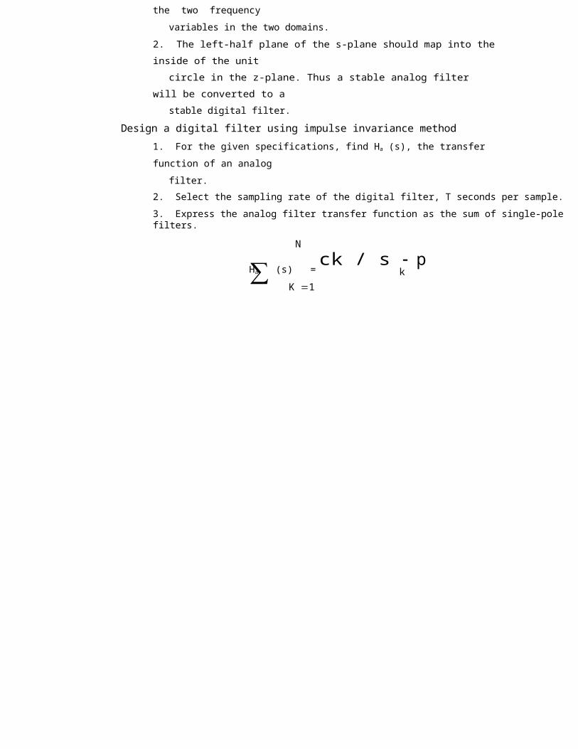
Design a digital filter using impulse invariance method

1. For the given specifications, find Ha (s), the transfer function of an analog

filter.

2. Select the sampling rate of the digital filter, T seconds per sample.

3. Express the analog filter transfer function as the sum of single-pole filters.

N

Ha (s) = ∑ K 1

ck / s pk

4. Compute the z-transform of the digital filter by using the formula

N

H (z) = ∑K 1

For high sampling rates use

N

c /1k

Tc

pkT 1e z

pkT 1/1 e z

H (z) = ∑ k K 1

Design digital filter using bilinear transform technique.

1. From the given specifications, find prewarping analog frequencies using formula Ω=

2/T tan w/2.

2. Using the analog frequencies find H (s) of the analog filter.

3. Select the sampling rate of the digital filter, call it T seconds per sample.

4. Substitute s= 2/T (1-z-1/1+ z-1) into the transfer function found in step2.

Program:

%Design of IIR Butterworth lowpass filter

alphap=input ('enter the pass band attenuation=');

alphas=input ('enter the stop band attenuation=');

fp=input ('enter the passband frequency=');

fs=input ('enter the stop band frequency=');

F=input ('enter the sampling frequency=');

omp=2*fp/F;

oms=2*fs/F;

[n, wn]=buttord (omp, oms, alphap, alphas) [b,

a]=butter (n, wn)

w=0:0.1: pi;

[h, ph]=freqz (b, a, w);

m=20*log (abs (h));

an=angle (h);

subplot (2, 1, 1);

plot (ph/pi, m);

grid on;

ylabel ('Gain in dB');


title (‘FREQUENCY RESPONSE OF BUTTERWORTH LOWPASS

subplot (2, 1, 2);

title (‘PHASE RESPONSE OF BUTTERWORTH LOWPASS FILTER’); plot

(ph/pi, an);

grid on;

ylabel ('Phase in Radians');


Output: Enter the pass band attenuation=

Enter the stop band attenuation=

Enter the pass band frequency=

Enter the stop band frequency=

Enter the sampling frequency=

n =

Wn =

b =

a =

Result:

Inference: There are no ripples in the passband and stopband.

Questions & Answers

1. What are the advantages of IIR filters (compared to FIR filters)? What are IIR

filters? What does "IIR" mean?

2. Why is the impulse response "infinite"?

3. What is the alternative to IIR filters?

4. What are the disadvantages of IIR filters (compared to FIR filters)?

b)

Aim: To design IIR Chebyshew type I high pass filter.

Program:

%Design of IIR Chebyshew type I high pass filter



fp=input ('enter the pass band frequency=');



omp=2*fp/F;

oms=2*fs/F;

[n, wn]=cheb1ord (omp, oms, alphap, alphas) [b,

a]=cheby1 (n, wn, high)

w=0:0.1: pi;


m=20*log (abs (h));

an=angle (h);

subplot (2, 1, 1);

plot (ph/pi, m);

grid on;



title (‘FREQUENCY RESPONSE OF CHEBYSHEW TYPE I HIGH PASS FILTER’);

subplot (2, 1, 2);

plot (ph/pi, an);

grid on;



title (‘PHASE RESPONSE OF CHEBYSHEW TYPE I HIGH PASS FILTER’);

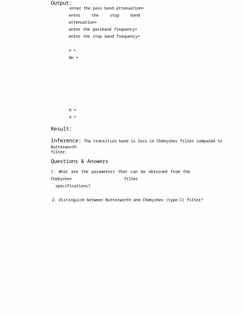
Output: enter the pass band attenuation=

enter the stop band attenuation=

enter the passband frequency=

enter the stop band frequency=

n =

Wn =

b =

a =

Result:

Inference: The transition band is less in Chebyshev filter compared to Butterworthfilter.

Questions & Answers

1. What are the parameters that can be obtained from the Chebyshev filter

specifications?

2. Distinguish between Butterworth and Chebyshev (type-I) filter?

6. N-POINT FFT ALGORITHM

Aim: To determine the N-point FFT of a given sequence.

Theory: The Fast Fourier transform is a highly efficient procedure for computing

the DFT of a finite series and requires less no of computations than that of direct

evaluation of DFT. It reduces the computations by taking the advantage of the fact

that the calculation of the coefficients of the DFT can be carried out iteratively. Due to

this, FFT computation technique is used in digital spectral analysis, filter simulation,

autocorrelation and pattern recognition. The FFT is based on decomposition and

breaking the transform into smaller transforms and combining them to get the total

transform. FFT reduces the computation time required to compute a discrete Fourier

transform and improves the performance by a factor 100 or more over direct

evaluation of the DFT. The fast fourier transform algorithms exploit the two basic

properties of the twiddle factor

k N

k N / 2(symmetry property: w N

k

w k N ,

periodicity property: w N w N ) and reduces the number of complex

multiplications required to perform DFT from N2 to N/2 log2N. In other words, for

N=1024, this implies about 5000 instead of 106 multiplications - a reduction factor of

200. FFT algorithms are based on the fundamental principal of decomposing the

computation of discrete fourier transform of a sequence of length N into successively

smaller discrete fourier transform of a sequence of length N into successively smaller

discrete fourier transforms. There are basically two classes of FFT algorithms. They

are decimation-in-time and decimation-in-frequency. In decimation-in-time, the

sequence for which we need the DFT is successively divided into smaller sequences

and the DFTs of these subsequences are combined in a certain pattern to obtain the

required DFT of the entire sequence. In the decimation-in-frequency approach, the

frequency samples of the DFT are decomposed into smaller and smaller

subsequences in a similar manner.

Radix - 2 DIT - FFT algorithm

1. The number of input samples N=2M , where, M is an integer.

2. The input sequence is shuffled through bit-reversal.

3. The number of stages in the flow graph is given by M=log2 N.

4. Each stage consists of N/2 butterflies.

5. Inputs/outputs for each butterfly are separated by 2m-1 samples, where m

represents the stage index, i.e., for first stage m=1 and for second stage m=2

so on.

6. The no of complex multiplications is given by N/2 log2 N.

7. The no of complex additions is given by N log2 N.

8. The twiddle factor exponents are a function of the stage index m and is given

by k Nt

mt 0,1,2,...2 m1

1. 2

9. The no of sets or sections of butterflies in each stage is given by the formula

2M-m.

10. The exponent repeat factor (ERF), which is the number of times the exponent

sequence associated with m is repeated is given by 2M-m.

Radix - 2 DIF - FFT Algorithm

1. The number of input samples N=2M, where M is number of stages.

2. The input sequence is in natural order.



5. Inputs/outputs for each butterfly are separated by 2M-m samples, Where m

represents the stage index i.e., for first stage m=1 and for second stage m=2

so on.

6. The number of complex multiplications is given by N/2 log2 N.

7. The number of complex additions is given by N log2 N.


by k 2

N t M m 1

mm,t 0,1,2,...2 1.

9. The number of sets or sections of butterflies in each stage is given by the

formula 2m-1.

10. The exponent repeat factor (ERF), which is the number of times the

exponent sequence associated with m repeated is given by 2m-1.

For decimation-in-time (DIT), the input is bit-reversed while the output is in natural order.

Whereas, for decimation-in-frequency the input is in natural order while the output is bit

reversed order.

The DFT butterfly is slightly different from the DIT wherein DIF the complex

multiplication takes place after the add-subtract operation.

Both algorithms require N log2 N operations to compute the DFT. Both algorithms

can be done in-place and both need to perform bit reversal at some place during the

computation.

Program: % N-point FFT algorithm

N=input ('enter N value=');

Xn=input ('type input sequence=');

k=0:1: N-1;

L=length (xn)

if (N<L)

error ('N MUST BE>=L');

end;

x1= [xn zeros (1, N-L)] for

c=0:1:N-1;

for n=0:1:N-1;

p=exp (-i*2*pi*n*C/N);

x2(c+1, n+1) =p;

end;

Xk=x1*x2';

end;

MagXk=abs (Xk);

angXk=angle (Xk);

subplot (2, 1, 1);

stem (k, magXk);

title ('MAGNITUDE OF DFT SAMPLES');

xlabel ('---->k');

ylabel ('-->Amplitude');

subplot (2, 1, 2);

stem (k, angXk);

title ('PHASE OF DFT SAMPLES');

xlabel ('---->k');

ylabel ('-->Phase');

disp (‘abs (Xk) =');

disp (magXk)

disp ('angle=');

disp (angXk)

Output: enter N value=

type input sequence=

L=

x1 =

abs (Xk) =

angle=

Result:

Inference: FFT reduces the computation time required to compute discreteFourier transform

Questions & Answers

1. What are the applications of FFT algorithms?

2. What is meant by radix-2 FFT?

3. What is an FFT "radix"?

4. What are "twiddle factors"?

5. What is an "in place" FFT?

6. What is "bit reversal"?

7. What is "decimation in time" versus "decimation in frequency"?

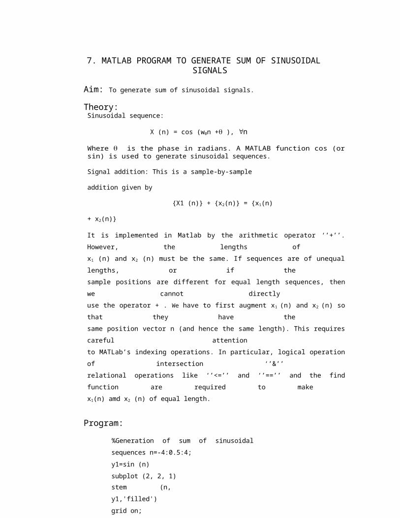
7. MATLAB PROGRAM TO GENERATE SUM OF SINUSOIDAL SIGNALS

Aim: To generate sum of sinusoidal signals.

Theory: Sinusoidal sequence:

X (n) = cos (w0n + ), n

Where is the phase in radians. A MATLAB function cos (or sin) is used to generate sinusoidal sequences.

Signal addition: This is a sample-by-sample addition given by

X1 (n) + x2(n) = x1(n) + x2(n)

It is implemented in Matlab by the arithmetic operator ‘’+’’. However, the lengths of

x1 (n) and x2 (n) must be the same. If sequences are of unequal lengths, or if the

sample positions are different for equal length sequences, then we cannot directly

use the operator + . We have to first augment x1 (n) and x2 (n) so that they have the

same position vector n (and hence the same length). This requires careful attention

to MATLab’s indexing operations. In particular, logical operation of intersection ‘’&’’

relational operations like ‘’<=’’ and ‘’==’’ and the find function are required to make

x1(n) amd x2 (n) of equal length.

Program:

%Generation of sum of sinusoidal sequences n=-

4:0.5:4;

y1=sin (n)

subplot (2, 2, 1)

stem (n, y1,'filled')

grid on;

xlabel ('-->Samples');

ylabel ('--->Magnitude');

title ('SINUSOIDAL SIGNAL1');

y2=sin (2*n)

subplot (2, 2, 2)

stem (n, y2,'filled')

grid on;



title ('SINUSOIDAL SIGNAL2');

y3=y1+y2

subplot (2, 1, 2);

stem (n, y3,'filled');



title ('SUM OF SINUSOIDAL SIGNALS');

Output:

Result:

Inference: The lengths of x1 (n) and x2 (n) must be the same for sample-by-sample addition.

Questions & Answers

1. What is deterministic signal? Give example.

2. Define a periodic signal?

8. MATLAB PROGRAM TO FIND FREQUENCY RESPONSE OF ANALOG LP/HP FILTERS.

a)

Aim: To find frequency response of Butterworth analog low pass filter.

Theory: The magnitude function of the butterworth lowpass filter is given by

H( j) 1/[1(/c2N 1/2

) ] N = 1, 2, 3, Where N is the order of the filter and Ωc is the cutoff frequency.The following expression is used for the order of the filter.

logN

10

10

log

0.1S

10.1P

1 S

P

Two properties of Butterworth lowpass filter

1. The magnitude response of the butterworth filter decreases

monotonically as the frequency Ω increases from 0 to ∞.

2. The magnitude response of the butterworth filter closely approximates

the ideal response as the order N increases.

3. The poles of the Butterworth filter lies on a circle.

Steps to design an analog butterworth lowpass filter

1. From the given specifications find the order of the filter N.

2. Round off it to the next higher integer.

3. Find the transfer function H (s) for Ωc = 1 rad/sec for the value of N.

4. Calculate the value of cutoff frequency Ωc.

5. Find the transfer function Ha (s) for the above value of Ωc by substituting

s s/Ωc in H(s).

Program:

%Design of Butterworth lowpass filter



fp=input ('enter the passband frequency=');



omp=2*fp/F;

oms=2*fs/F;

[N, wn]=buttord (omp, oms, alphap, alphas,'s') [b,

a]=butter (n, wn)

w=0:0.01: pi;


m=20*log (abs (h));

an=angle (h);

subplot (2, 1, 1);

plot (ph/pi, m);

grid on;


xlabel ('Normalised Frquency');

title ('FREQUENCY RESPONSE OF BUTTERWORTH LOWPASS FILTER');

subplot (2, 1, 2);

plot (ph/pi, an);

grid on;


xlabel ('Normalisd Frequency');

title ('PHASE RESPONSE OF BUTTERWORTH LOWPASS FILTER');

Output:

Enter the pass band attenuation=




Enter the sampling frequency=

n =

Wn =

b =

a =

Result:

Inference: The magnitude response of the butterworth filter decreases monotonically as the frequency increases.

Questions & Answers

1. Give any two properties of Butterworth lowpass filters?

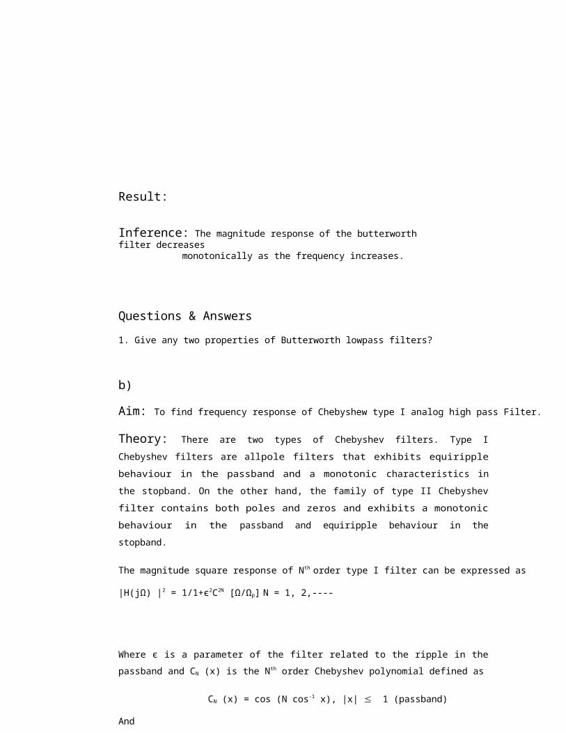
b)

Aim: To find frequency response of Chebyshew type I analog high pass Filter.

Theory: There are two types of Chebyshev filters. Type I Chebyshev filters are allpole

filters that exhibits equiripple behaviour in the passband and a monotonic

characteristics in the stopband. On the other hand, the family of type II Chebyshev filter

contains both poles and zeros and exhibits a monotonic behaviour in the passband

and equiripple behaviour in the stopband.

The magnitude square response of Nth order type I filter can be expressed as

|H(jΩ) |2 = 1/1+є2C2N [Ω/Ωp] N = 1, 2,----

Where є is a parameter of the filter related to the ripple in the passband and CN (x) is the Nth

order Chebyshev polynomial defined as

CN (x) = cos (N cos-1 x), |x| 1 (passband)

And CN (x) = cosh (N cosh-1 x), |x| > 1 (stopband)

Steps to design an analog Chebyshev lowpass filter

1. From the given specifications find the order of the filter N.

2. Round off it to the next higher integer.

3. Using the following formulas find the value of a and b, which are minor and

major axis of the ellipse respectively.

a = Ωp [µ1/N - µ-1/N]

2 ;

b=Ωp [µ1/N - µ-1/N]

2

Where µ = є-1 + є-2 + 1

Є = 100.1 p - 1

Ωp = passband frequency

p= Maximum allowable attenuation in the passband

(For normalized Chebyshev filter Ωp = 1 rad/sec)

4. Calculate the poles of Chebyshev filter which lies on an ellipse by using the formula.

Sk = a cosФk + jb sin Фk k= 1, 2, .N

Where Фk = /2 + [2k-1/2N] k= 1, 2, .N

5. Find the denominator polynominal of the transfer function using above poles.

6. The numerator of the transfer function depends on the value of N.

a) For N odd substitute s = 0 in the denominator polynominal and find

the value. This value is equal to the numerator of the transfer

function.

(For N odd the magnitude response |H(jΩ)| starts at 1.)

b) For N even substitute s=0 in the denominator polynominal and divide

the result by 1+ Є2. This value is equal to the numerator.

The order N of Chebyshev filter is given by

N= cos h-1 [(100.1 s -1)/ (100.1 p -1)]/cos h-1 ( s/ p)

s and p

Where s is stopband attenuation at stopband frequency is passbandattenuation at passband frequency p . The major minor axis of the ellipse is givenby

b= p [(µ1/N + µ-1/N )/2] and a = p [ (µ1/N - µ-1/N )/2]

Where µ = Є-1 + 1+ Є-2

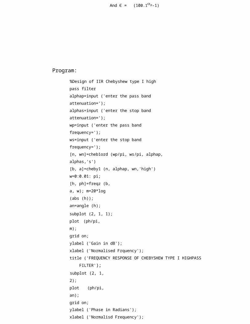
And Є = (100.1 p-1)

Program:

%Design of IIR Chebyshew type I high pass filter



wp=input ('enter the pass band frequency=');

ws=input ('enter the stop band frequency=');

[n, wn]=cheb1ord (wp/pi, ws/pi, alphap, alphas,'s')

[b, a]=cheby1 (n, alphap, wn,'high')

w=0:0.01: pi;


m=20*log (abs (h));

an=angle (h);

subplot (2, 1, 1);

plot (ph/pi, m);

grid on;


xlabel ('Normalised Frquency');

title ('FREQUENCY RESPONSE OF CHEBYSHEW TYPE I HIGHPASS

FILTER');

subplot (2, 1, 2);

plot (ph/pi, an);

grid on;


xlabel ('Normalisd Frequency');

title ('PHASE RESPONSE OF CHEBYSHEW TYPE I HIGHPASS FILTER');

Output:

Enter the pass band attenuation=




n =

wn =

b =

a =

Result:

Inference: Chebyshev approximation provides better characteristics near the cutoff frequency and near the stop band edge.

Questions & Answers

1. How one can design digital filters from analog filters?

2. What are the properties of Chebyshev filter?

9. POWER DENSITY SPECTRUM OF A SEQUENCE

Aim: To compute power density spectrum of a sequence.

Theory: PSD Power Spectral Density estimate.

Pxx = PSD(X, NFFT, Fs, WINDOW) estimates the Power Spectral Density of

a discrete-time signal vector X using Welch's averaged, modifiedperiodogram

method.X is divided into overlapping sections, each of which is detrended (according

to the detrending flag, if specified), then windowed by the WINDOW parameter, then

zero-padded to length NFFT. The magnitude squared of the length NFFT DFTs of

the sections are averaged to form Pxx. Pxx is length NFFT/2+1 for NFFT even,

(NFFT+1)/2 for NFFT odd, or NFFT if the signal X is complex. If you specify a scalar

for WINDOW, a Hanning window of that length is used. Fs is the sampling frequency

which doesn't affect the spectrum estimate but is used for scaling the X-axis of the

plots. [Pxx, F] = PSD(X, NFFT, Fs, WINDOW, NOVERLAP) returns a vector of

frequencies the same size as Pxx at which the PSD is estimated, and overlaps

the sections of X by NOVERLAP samples. [Pxx, Pxxc, F] = PSD(X, NFFT, Fs,

WINDOW, NOVERLAP, P) where P is a scalar between 0 and 1, returns the P*100%

confidence interval for Pxx. PSD(X, DFLAG), where DFLAG can be 'linear', 'mean' or

'none', specifies a detrending mode for the prewindowed sections of X. DFLAG can

take the place of any parameter in the parameter list (besides X) as long as it is last,

e.g. PSD(X,'mean'); PSD with no output arguments plots the PSD in the current

figure window, with confidence intervals if you provide the P parameter. The default

values for the parameters are NFFT = 256 (or LENGTH(X), whichever is smaller),

NOVERLAP = 0, WINDOW = HANNING (NFFT), Fs = 2, P = .95, and DFLAG =

'none'. You can obtain a default parameter by leaving it off or inserting an empty

matrix [], e.g. PSD(X, [], 10000).

Program: %Power density spectrum of a sequence

x=input ('enter the length of the sequence=');

y=input ('enter the sequence=');

fs=input ('enter sampling frequency=');

N=input ('enter the value of N=');

q=input ('enter the window name1=');

m=input ('enter the window name2=');

s=input ('enter the window name3=');

pxx1=psd(y, N, fs, q)

plot (pxx1,'c');

hold on;

grid on;

pxx2=psd(y, N, fs, m)

plot (pxx2,'k');

hold on;

pxx3=psd(y, N, fs, s)

plot (pxx3,'b');

hold on;

xlabel ('-->Frequency');

ylabel ('-->Magnitude');

title ('POWER SPECTRAL DENSITY OF A SEQUENCE');

hold off;

Output: Enter the length of the sequence=

Enter the sequence=

Enter sampling frequency=

Enter the value of N=

Enter the window name1=



pxx1 =

pxx2 =

pxx3 =

Result:

Inference: Power spectral density does not have any phase information.

Questions & Answers

1. Define power spectral density?

2. What is window function? What are the applications of window functions?

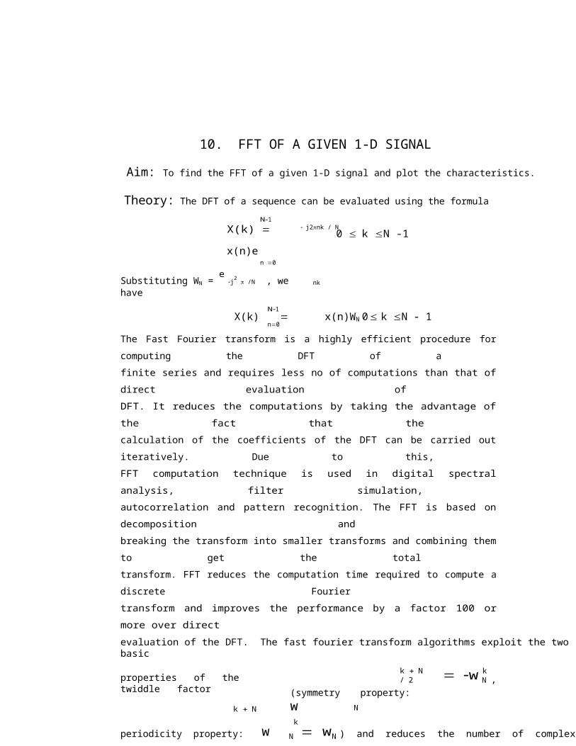
10. FFT OF A GIVEN 1-D SIGNAL

Aim: To find the FFT of a given 1-D signal and plot the characteristics.

Theory: The DFT of a sequence can be evaluated using the formula

N1

X(k) x(n)en 0

Substituting WN = e

j2 /N , we have

N1

j2nk / N0 k N -1

nk X(k) x(n)WN 0 k N - 1

n0

The Fast Fourier transform is a highly efficient procedure for computing the DFT of a

finite series and requires less no of computations than that of direct evaluation of

DFT. It reduces the computations by taking the advantage of the fact that the

calculation of the coefficients of the DFT can be carried out iteratively. Due to this,

FFT computation technique is used in digital spectral analysis, filter simulation,

autocorrelation and pattern recognition. The FFT is based on decomposition and

breaking the transform into smaller transforms and combining them to get the total

transform. FFT reduces the computation time required to compute a discrete Fourier

transform and improves the performance by a factor 100 or more over direct

evaluation of the DFT. The fast fourier transform algorithms exploit the two basic

properties of the twiddle factor

k N

k N / 2

(symmetry property: w N

k

w k N ,

periodicity property: w N w N ) and reduces the number of complex

multiplications required to perform DFT from N2 to N/2 log2N. In other words, for

N=1024, this implies about 5000 instead of 106 multiplications - a reduction factor of

200. FFT algorithms are based on the fundamental principal of decomposing the

computation of discrete fourier transform of a sequence of length N into successively

smaller discrete fourier transform of a sequence of length N into successively smaller

discrete fourier transforms. There are basically two classes of FFT algorithms. They

are decimation-in-time and decimation-in-frequency. In decimation-in-time, the

sequence for which we need the DFT is successively divided into smaller sequences

and the DFTs of these subsequences are combined in a certain pattern to obtain the

required DFT of the entire sequence. In the decimation-in-frequency approach, the

frequency samples of the DFT are decomposed into smaller and smaller

subsequences in a similar manner.

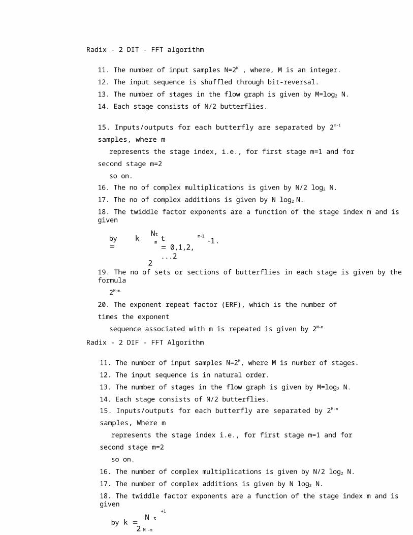
Radix - 2 DIT - FFT algorithm

11. The number of input samples N=2M , where, M is an integer.

12. The input sequence is shuffled through bit-reversal.



15. Inputs/outputs for each butterfly are separated by 2m-1 samples, where m

represents the stage index, i.e., for first stage m=1 and for second stage m=2

so on.

16. The no of complex multiplications is given by N/2 log2 N.

17. The no of complex additions is given by N log2 N.


by k Nt

mt 0,1,2,...2 m1

1. 2

19. The no of sets or sections of butterflies in each stage is given by the formula

2M-m.

20. The exponent repeat factor (ERF), which is the number of times the exponent

sequence associated with m is repeated is given by 2M-m.

Radix - 2 DIF - FFT Algorithm

11. The number of input samples N=2M, where M is number of stages.

12. The input sequence is in natural order.



15. Inputs/outputs for each butterfly are separated by 2M-m samples, Where m

represents the stage index i.e., for first stage m=1 and for second stage m=2

so on.

16. The number of complex multiplications is given by N/2 log2 N.

17. The number of complex additions is given by N log2 N.


by k 2

N t M m 1

mm,t 0,1,2,...2 1.

19. The number of sets or sections of butterflies in each stage is given by the

formula 2m-1.

20. The exponent repeat factor (ERF),Which is the number of times the exponent

sequence associated with m repeated is given by 2m-1.

Program:

%To find the FFT of a given 1-D signal and plot

N=input ('enter the length of the sequence=');

M=input ('enter the length of the DFT=');

u=input ('enter the sequence u (n) =');

U=fft (u, M)

A=length (U)

t=0:1: N-1;

subplot (2, 2, 1);

stem (t, u);

title ('ORIGINAL TIME DOMAIN SEQUENCE');

xlabel ('---->n');


subplot (2, 2, 2);

k=0:1:A-1;

stem (k, abs (U));

disp (‘abs (U) =');

disp (abs (U))

title ('MAGNITUDE OF DFT SAMPLES');

xlabel ('---->k');


subplot (2, 1, 2);

stem (k, angle (U));

disp (‘angle (U) =')

disp (angle (U))

title ('PHASE OF DFT SAMPLES');

xlabel ('---->k');

ylabel ('-->phase');

Output: Enter the length of the sequence=

Enter the length of the DFT=

Enter the sequence u (n) =

U =

A =

abs (U) =

angle (U) =

Result:

Inference: FFT reduces the computation time required to compute discrete Fourier transform.

Questions & Answers

1. What is the FFT?

2. How does the FFT work?

3. How efficient is the FFT?

4. Are FFT's limited to sizes that are powers of 2?

OTHER EXPERIMENTS

1. GENERATION OF BASIC SEQUENCES

Aim: To generate impulse, step and sinusoidal sequences.

Program:

%Generation of basic sequences

%generation of impulse sequence

t=-2:1:2;

v= [zeros (1, 2), ones (1, 1), zeros (1, 2)]

subplot (2, 2, 1);

stem (t, v,'m','filled');

grid on;


xlabel ('--->n');

title (' IMPULSE SEQUENCE');

%generation of step sequence

t=0:1:5;

m= [ones (1, 6)]

subplot (2, 2, 2);

stem (t, m,'m','filled');

grid on;


xlabel ('--->n');

title (' STEP SEQUENCE');

%generation of sinusoidal sequence

t=-4:1:4;

y=sin (t)

subplot (2, 1, 2);

stem (t, y,'m','filled');

grid on;


xlabel ('--->n');

title ('SINUSOIDAL SEQUENCE');

Output: v =

m =

y=

Result:

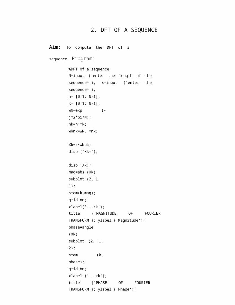
2. DFT OF A SEQUENCE

Aim: To compute the DFT of a sequence.

Program:

%DFT of a sequence

N=input ('enter the length of the sequence=');

x=input ('enter the sequence=');

n= [0:1: N-1];

k= [0:1: N-1];

wN=exp (-j*2*pi/N);

nk=n'*k;

wNnk=wN. ^nk;

Xk=x*wNnk;

disp ('Xk=');

disp (Xk);

mag=abs (Xk)

subplot (2, 1, 1);

stem(k,mag);

grid on;

xlabel('--->k');

title ('MAGNITUDE OF FOURIER TRANSFORM');

ylabel ('Magnitude');

phase=angle (Xk)

subplot (2, 1, 2);

stem (k, phase);

grid on;

xlabel ('--->k');

title ('PHASE OF FOURIER TRANSFORM');

ylabel ('Phase');

Output:

Enter the length of the sequence=

Enter the sequence=

Xk=

mag =

phase =

Result:

3. IDFT OF A SEQUENCE

Aim: To compute the IDFT of a sequence.

Program:

%IDFT of a sequence

Xk=input (‘enter X (K) ='); [N,

M]=size (Xk);

if M~=1;

Xk=Xk.';

N=M;

end;

xn=zeros (N, 1);

k=0: N-1;

for n=0: N-1;

xn (n+1) =exp (j*2*pi*k*n/N)*Xk;

end;

xn=xn/N;

disp (‘x (n) = ');

disp (xn);

plot (xn);

grid on;

plot(xn);

stem(k,xn);

xlabel ('--->n');

ylabel ('-->magnitude');

title (‘IDFT OF A SEQUENCE’);

Output:

Enter the dft of X (K) =

x (n) =

Result:

CODE COMPOSER STUDIO

TEXAS INSTRUMENT DSP STARTER KIT 6711DSK A BRIEF INTRODUCTION

1 Introduction

The purpose of this documentation is to give a very brief overview of the structure of the

6711DSK. Included is also a mini tutorial on how to program the DSP, download programs

and debug it using the Code Composer Studio software.

2 The DSP starter kit

The Texas Instrument 6711DSK is a DSP starter kit for the TMS320C6711 DSP chip. The kit

contains:

• An emulator board which contains:

- DSP chip, memory and control circuitry.

- Input/output capabilities in the form of

_ An audio codec (ADC and DAC) which provides 1 input and 1 output

channel sampled at 8 kHz.

_ Digital inputs and outputs

_ A connector for adding external evaluation modules, like the PCM3003

Audio daughter card which has 2 analog in and 2 analog out sampled at

48 kHz.

- A parallel port for interface to a host computer used for program

development, program download and debugging.

• The Code Composer Studio (CCS) software which is an integrated development

environment (IDE) for editing programs, compiling, linking, download to target

(i.e., to the DSK board) and debugging. The CCS also includes the DSP/BIOS

real-time operating system. The DSP/BIOS code considerably simplifies the code

development for real-time applications which include interrupt driven and time

scheduled tasks.

3 Usage overview

Working with the DSK involves the following steps:

• The first step is the algorithm development and programming in C/C++ or

assembler. We will only consider coding in C in this document. The program is typed using

the editor capabilities of the CCS. Also the DSP/BIOS configuration is performed in a

special configuration window.

• When the code is finished it is time to compile and link the different code parts

together. This is all done automatically in CCS after pressing the Build button. If

the compilation and linking succeeded the finished program is downloaded to the

DSK board.

• The operation of DSK board can be controlled using CCS, i.e., CCS also works as a

debugger. The program can be started and stopped and single-step. Variables in the

program can be inspected with the “Watch” functionality. Breakpoints can be inserted in

the code.

4 Getting started with the 6711DSK and CCS

In this section you will be introduced to the programming environment and will

download and execute a simple program on the DSK.

4.1 Connecting the PC and DSK

The DSK is communicating with the host PC using the parallel-port interface.

1. Start Code Composer Studio (CCS) by clicking on the “CCStudio 3.01” icon on the workspace.

2. Check that the DSK is powered up. If not, power up the DSK by inserting the AC power cable (mains) to the black AC/DC converter. Note: Never unplug the power cable from the DSK card.

3. Make a connection between CCS and the DSK by selecting menu command Debug! Connect. If connection fails perform following steps:

(a) Select menu command Debug! Reset Emulator

(b) Power cycle the DSK by removing the AC power cord from the AC/DC converter, wait about a second and then reinsert.

(c) Select menu command Debug! Connect.

4.2 Getting familiar with CCS

CCS arranges its operation around a project and the “Project view” window is

displayed to the left. Here you can find all files which are related to a certain project. At the

bottom of the CCS window is the status output view in which status information will be

displayed such as compile or link errors as well as other types of information. Note that the

window will have several tabs for different types of output.

4.3 Loading programs from CCS

One setting might need to be changed in CCS in order to automatically download the

program after compilation and linking (a build). You find the setting under menu

command Options! Customize and tab Program Load Options. Tick the box Load

Program after Build.

4.3.1 Project view and building an application

You open an existing project by right-clicking on the project folder and select the

desired “.pjt” file or select the command from the menu Project! Open...........

• Open the project “intro.pjt” which you find in the “intro”folder.

• Press the “+” sign to expand the view. Several folders appear which contain all the

project specific files.

• Open up the Source folder. Here you will find all the files with source code which

belongs to the project.

• Double click on the “intro.c” file to open up an editor window with the file “intro.c” file

loaded.

• Look around in the file. The code calculates the inner product between two integer

vectors of length “COUNT” by calling the function “dotp” and then prints the result using

the “LOG printf” command.

• Compile, link and download the code selecting the Project! Build command or use

the associated button. If the download fails. Power cycle the DSK and retry Project!

Build.

4.3.2 Running the code after a successful build command (compile, link and

download) the program is now resident in the DSK and ready for execution. A

disassembly window will appear showing the Assembly language instructions

produced by the compiler. You can minimize the window for now. At the bottom left

you will see the status “CPU HALTED” indicating that the CPU is not executing any

code. A few options are available depending on if you want to debug or just run the

code.

To simply run the code does:

• Select Debug! Run to start the execution. At the bottom left you will see the status “CPU

RUNNING” indicating that the program is executed.

• To stop the DSP select Debug! Halt.

• If you want the restart the program do Debug! Restart followed by Debug! Run

Try to run the code in the intro project. To see the output from the LOG printf

commands you must enable the view of the Message Log Window. Do DSP/BIOS!

Message Log and select LOG0 in the pull-down menu.

4.3.3 CCS Debug

Single stepping for debugging the code do the following:

• Select Debug! Go Main. This will run DSP/BIOS part of the code until the start

of the “main” function. A yellow arrow will appear to the left of the start of the

“main” function in the edit window for the “intro.c” file. The arrow indicates where

the program execution has halted.

• Now you can step the code one line at the time. Three commands are available:

- Debug! Step Into will execute the marked line if it is composed of simple

instructions or if the line has a function call, will step in to the called function.

- Debug! Step Over will execute the marked line and step to the next line.

- Debug! Step Out will conclude the execution of the present function and halt

the execution at the next line of the calling function. Try to step through the code

using the step functions. View variables if you want to know the value of a particular

variable just put the cursor on top of the variable in the source window. The value will

after a short delay pop up next to the variable. Note that local variables in functions

only have defined values when the execution is located inside the function. Variables

can also be added to the “Watch window” which enables a concurrent view of several

variables. Mark the “y” variable in source code, right-click and select Add to Watch

Window. The watch window

will then add variable “y” to the view and show its contents. Also add the “a” variable (which

is a array) to the watch window. Since “a” is an array the value of “a” is an address. Click

on the “+”. This will show the individual values of the array. The watch window will update

its contents whenever the DSP is halted. It is also possible to change the value of a

variable in the DSK from the Watch window. Simply select the numerical value you want to

change and type in a new value. CCS will send the new value to the DSK before starting the

execution.

Break points Break points can also be used to halt the execution at a particular point

in the source code. To illustrate its use consider the “intro”. Place the cursor at the

line which has the “return (sum);” instruction in the “dotp” function. Right-click and

select Toggle breakpoint. A red dot will appear at that line indicating that a breakpoint

is set at that line. Try it out. First do Debug! Restart and then Debug! Run The

execution will halt at the line and we can investigate variables etc. To resume

execution simply issue Debug! Run command again. Shortcut buttons CCS offers a

number of shortcut buttons both for the build process as well as the debugging.

Browse around with the mouse pointer to find them. The balloon help function will

show what command a particular button is associated with, i.e., move the mouse

pointer over a button and wait for the balloon help to show up. Loading the values in

a vector into Matlab In the Lab you will need to load the coefficients of a FIR filter into

Matlab for further analysis. The filter coefficients are stored in vectors. Use the

following procedure:

1. Run the DSP program on the DSK.

2. Halt the execution when it is time to upload the vector.

3. In the File menu you find File! Data! Save In the file dialog assign a name to the

data file and select ”Float” as ”Save as type”.

4. In the next dialog enter the name of the vector in the address field. When you tab away

from it it will change to the absolute memory address of the vector. In the length box

you enter the length of the variable. Note that you need to remove the 0x prefix if you give

the length using decimals numbers. The notation with 0x in the beginning indicates

that the number is a Hexadecimal number, i.e. it is based on a base of 16 instead of the

normal base of 10 in the decimal system.

5. Open the file in an editor and remove the first line and save again

6. In Matlab use the ”load” command to load the saved file. The vector will get the same

name as the file name without the extension.

5 Debugging - limitations

The debugging features of the CCS are very handy during the code development.

However, several limitations are present.

• Since the compiler will optimize the code, all lines in the C-code cannot be used as

breakpoints. Since the architecture has several parallel processing units the final code

might execute several lines of C in one clock cycle.

• The processor also has memory cache which speeds up normal operations. This

means that when the DSP loads a particular memory location it will copy it into

the cache memory and then perform the operations (faster) using the cache. After some

time the cache will be written back again to the memory. This can sometimes confuse CCS

and variables in the Watch window can be erroneous.

• The third important issue is when debugging code which is dependent on external

events, e.g., interrupt driven code. When halting such a code by a break point

several features are important to consider. Firstly, since the code is stopped all realtime

deadlines will be broken so future sampled inputs will be lost. Hence a restart from the

point of the break might cause unpredicted behavior.

• Sometimes the code in the DSK which communicates with the CCS stops working.

When this happens it is necessary to power cycle, the DSK board in order to restart

the operation. Sometimes it is also necessary at the same time to restart CCS.

PROCEDURE TO WORK ON CODE COMPOSER STUDIO

To create the new project Project new (File name.pjt, eg: vectors.pjt)

To create a source file File new type the code (save &give file name, eg: sum.c

To add source files to project Project add files to project sum.c

To add rts.lib file&hello.cmd: Project add files to project rts6700.lib

Libraryfiles: rts6700.lib (path:c:\ti\c6000\cgtools\lib\rts6700.lib) Note: select object&library in (*.o,*.1) in type of files

Project add files to projects hello.cmd

Cmd file - which is common for all non real time programs. (path:c\ti\tutorials\dsk6711\hello.1\hello.cmd)

Note: select linker command file (*.cmd) in type of files

Compile:

To compile: project compile

To rebuild: project rebuild

Which will create the final.outexecutablefile (eg.vectors.out)

Procedure to load and run program:

Load the program to DSK: file load program vectors. Out To

execute project: Debug run

C PROGRAMS (USING64XX, 67XX SIMULATORS)


Aim: Write a C program for linear convolution of two discrete sequences and

compute using code composer studio V2 (using simulators 64xx, 67xx, 6711)

software.

Program: #include<stdio.h>

#include<math.h>

main ()

int x[20],h[20],y[20],N1,N2,n,m;

printf ("enter the length of the sequence x (n) :");

scanf ("%d", &N1);

printf ("enter the length of the sequence h (n) :");

scanf ("%d", &N2);

printf ("enter the sequence x (n) :"); for

(n=0; n<N1; n++)

scanf ("%d", &x[n]);

printf ("enter the sequence h (n) :"); for

(n=0; n<N2; n++)

scanf ("%d", &h[n]);

for (n=0; n<N1+N2-1; n++)

if (n>N1-1)

y[n]=0; for(m=n-(N1-1);m<=(N1-1);m++) y[n] =y[n] +x[m]*h [n-m];

else

y[n] =0; for (m=0; m<=n; m++)y[n] =y[n] +x[m]*h [n-m];

printf ("convolution of two sequences is y (n) :"); for (n=0; n<N1+N2-1; n++) printf ("%d\t", y[n]);

Input:

Enter the length of the sequence x (n):

Enter the length of the sequence h (n):

Enter the sequence x (n):

Enter the sequence h (n):

Output:

Convolution of two sequences is y (n):

Result:


Aim: Write a C program for circular convolution of two discrete sequences and

compute using code composer studio V2 (using simulators 64xx, 67xx, 6711)

software.

Program:

#include<math.h>

#define pi 3.14

main ()

int x[20],h[20],y[20],N1,N2,N,n,m,k;


scanf ("%d", &N1);


scanf ("%d", &N2);

printf ("enter the %d samples of sequence x (n):” N1); for

(n=0; n<N1; n++)


printf ("enter the %d samples of sequence h (n):” N2); for

(n=0; n<N2; n++)

scanf ("%d", &h[n]); if

(N1>N2)

N=N1;

for (n=N2; n<N; n++)

h[n]=0;

else

N=N2;

for(n=N1;n<N1;n++)

y[n]=0;

for(k=0;k<N;k++)

y[k]=0;

for (m=N-1; m>=0; m--)

if ((N+k-m)>=N)

y[k] =y[k] +x[m]*h [k-m];

else

y[k] =y[k] +x[m]*h [N+k-m];

printf ("\response is y (n) :"); for

(n=0; n<N; n++)

printf ("\t%d", y[n]);

Input:



Enter the 4 samples of sequence x (n):

Enter the 4 samples of sequence h (n):

Output:

Response is y (n):

Result:

3. DFT OF A SEQUENCE

Aim: Write a C program for DFT of a sequence and compute using code composer

studio V2 (using simulators 64xx, 67xx, 6711) software.

Program:

%DISCRETE FOURIER TRANSFORM OF THE GIVEN SEQUENCE

#include<stdio.h>

#include<math.h>

#define pi 3.14

main ()

int x [20], N, n, k;

float Xre[20],Xim[20],Msx[20],Psx[20];


scanf ("%d", &N);

printf ("enter the %d samples of discrete sequence x (n):” N); for

(n=0; n<N; n++)


for(k=0;k<N;k++)

Xre[k]=0;

Xim[k]=0;

for(n=0;n<N;n++)

Xre[k]=Xre[k]+x[n]*cos(2*pi*n*k/N);

Xim[k]=Xim[k]+x[n]*sin(2*pi*n*k/N);

Msx[k]=sqrt(Xre[k]*Xre[k]+Xim[k]*Xim[k]);

Xim[k]=-Xim[k];

Psx[k]=atan(Xim[k]/Xre[k]);

printf ("discrete sequence is");

for (n=0; n<N; n++)

printf ("\nx(%d) =%d", n,x[n]);

printf ("\nDFT sequence is :");

for(k=0;k<N;k++)

printf("\nx(%d)=%f+i%f",k,Xre[k],Xim[k]);

printf("\nmagnitude is:");

for (k=0; k<N; k++)

printf ("\n%f",Msx[k]);

printf ("\nphase spectrum is");

for(k=0;k<n;k++)

printf("\n%f",Psx[k]);

Input: Enter the length of the sequence x (n):

Enter the 4 samples of discrete sequence x (n):

Output:

Discrete sequence is:

x (0) =

x(1) =

x(2) =

x (3) =

DFT sequence is :

x(0)=

x(1)=

x(2)=

x (3) =

Magnitude is: Phase spectrum is:

Result:

4. IDFT OF A SEQUENCE

Aim: Write a C program for IDFT of a sequence and compute using code composer studio

V2 (using simulators 64xx, 67xx, 6711) software.

Program:

% Inverse Discrete Foureir Transform

#include<stdio.h>

#include<math.h>

#define pi 3.1428

main()

int j, k, N, n;

float XKr[10],XKi[10],xni[10],xnr[10],t;

printf (" enter seq length: \n");

scanf ("%d", &N);

printf ("enter the real & imaginary terms of the sequence: \n"); for

(j=0; j<N; j++)

scanf ("%f%f", &XKr[j], &XKi[j]);

for (n=0; n<N; n++)

xnr[n] =0; xni[n] =0; for(k=0;k<N;k++)

t=2*pi*k*n/N;

xnr[n]=( xnr[n]+XKr[k]*cos(t) - XKi[k]*sin(t)) ;

xni[n]=( xni[n]+XKr[k]*sin(t) + XKi[k]*cos(t)) ;

xnr[n]=xnr[n]/N;

xni[n]=xni[n]/N;

printf("IDFT seq:");

for(j=0;j<N;j++)

printf("%f + (%f) i\n",xnr[j],xni[j]);

Input:

Enter seq length:

Enter the real & imaginary terms of the sequence:

Output:

IDFT seq:

Result:

5. N - POINT DISCRETE FOUREIR TRANSFORM

Aim: Write a C program for N - Point Discrete Foureir Transform of a sequence

and compute using code composer studio V2( using simulators 64xx,67xx,6711)

software.

Program:

% N - Point Discrete Foureir Transform

#include<stdio.h>

#include<math.h>

#define pi 3.142857

main ()

int j, k, n, N, l;



scanf ("%d", &l);


(j=0; j<l; j++)

scanf ("%f%f", &xnr[j], &xni[j]);

printf (" enter required length: \n");

scanf ("%d", &N);

if (l<N)

for(j=l;j<N;j++)

xnr[j]=xni[j]=0;

for(k=0;k<N;k++)

XKr[k]=0; XKi[k]=0;

for(n=0;n<N;n++)

t=2*pi*k*n/N;

XKr[k]=( XKr[k]+xnr[n]*cos(t) + xni[n]*sin(t)) ;

XKi[k]=( XKi[k]+ xni[n]*cos(t) - xnr[n]*sin(t)) ;

printf (" The %d Point DFT seq:” N);

for(j=0;j<N;j++)

printf("%3.3f + (%3.3f) i\n",XKr[j],XKi[j]);

Input:

Enter seq length:


enter required length:

Out put:

The 4 Point DFT seq:

Result:

6. TO GENERATE SUM OF SINUSOIDAL SIGNALS

Aim: Write a C program to generate sum of sinusoidal signals and compute using code

composer studio V2 (using simulators 64xx, 67xx, 6711) software.

Program:

%SUM OF TWO SINUSOIDALS

#include<stdio.h>

#include<math.h>

main ()

int w1, w2, t;

float a, b, c;

printf ("enter the w1 value:");

scanf ("%d", &w1);

printf ("enter the w2 value:");

scanf ("%d", &w2);

printf ("sum of two sinusoidal :");

for(t=-5;t<5;t++)

b=sin(w1*t);

c=sin (w2*t);

a=b+c;

printf ("\n%f", a);

Input: Enter the w1 value:

Enter the w2 value:

Output:

Sum of two sinusoidal:

Result:

PROGRAMS USING TMS 320C 6711 DSK


Aim: Write a C program for linear convolution of two discrete sequences and

compute using TMS 320C 6711 DSK.

Program: #include<stdio.h>

#include<math.h>

main ()

int x[20],h[20],y[20],N1,N2,n,m;


scanf ("%d", &N1);


scanf ("%d", &N2);

printf ("enter the sequence x (n) :"); for

(n=0; n<N1; n++)


printf ("enter the sequence h (n) :"); for

(n=0; n<N2; n++)

scanf ("%d", &h[n]);

for (n=0; n<N1+N2-1; n++)

if (n>N1-1)

y[n]=0;

for(m=n-(N1-1);m<=(N1-1);m++) y[n]

=y[n] +x[m]*h [n-m];

else

y[n] =0;

for (m=0; m<=n; m++)

y[n] =y[n] +x[m]*h [n-m];

printf ("convolution of two sequences is y (n) :");

for (n=0; n<N1+N2-1; n++)

printf ("%d\t", y[n]);

Input:



Enter the sequence x (n):

Enter the sequence h (n):

Output:

Convolution of two sequences is y (n):

Result:


Aim: Write a C program for circular convolution of two discrete sequences and

compute using using TMS 320C 6711 DSK.

Program:

#include<math.h>

#define pi 3.14

main ()

int x[20],h[20],y[20],N1,N2,N,n,m,k;


scanf ("%d", &N1);


scanf ("%d", &N2);

printf ("enter the %d samples of sequence x (n):", N1); for

(n=0; n<N1; n++)


printf ("enter the %d samples of sequence h (n):” N2); for

(n=0; n<N2; n++)

scanf ("%d", &h[n]); if

(N1>N2)

N=N1;

for (n=N2; n<N; n++)

h[n]=0;

else

N=N2;

for(n=N1;n<N1;n++)

y[n]=0;

for(k=0;k<N;k++)

y[k]=0;

for (m=N-1; m>=0; m--)

if ((N+k-m)>=N)

y[k] =y[k] +x[m]*h [k-m];

else

y[k] =y[k] +x[m]*h [N+k-m];

printf ("\response is y (n) :"); for

(n=0; n<N; n++)

printf ("\t%d", y[n]);

Input:



Enter the 4 samples of sequence x (n):

Enter the 4 samples of sequence h (n):

Output:

Response is y (n):

Result:

3. FINDING DFT OF A SEQUENCE

Aim: Write a C program for DFT of a sequence and compute using TMS 320C 6711

DSK.

Program:

%DISCRETE FOURIER TRANSFORM OF THE GIVEN SEQUENCE

#include<stdio.h>

#include<math.h>

#define pi 3.14

main ()

int x [20], N, n, k;

float Xre[20],Xim[20],Msx[20],Psx[20];


scanf ("%d", &N);

printf ("enter the %d samples of discrete sequence x (n):” N); for

(n=0; n<N; n++)


for(k=0;k<N;k++)

Xre[k]=0;

Xim[k]=0;

for(n=0;n<N;n++)

Xre[k]=Xre[k]+x[n]*cos(2*pi*n*k/N);

Xim[k]=Xim[k]+x[n]*sin(2*pi*n*k/N);

Msx[k]=sqrt(Xre[k]*Xre[k]+Xim[k]*Xim[k]);

Xim[k]=-Xim[k];

Psx[k]=atan(Xim[k]/Xre[k]);

printf ("discrete sequence is:");

for (n=0; n<N; n++)

DIGITAL SIGNAL PROCESSING LAB 113

ELECTRONICS & COMMUNICATION ENGINEERING

printf ("\nx (%d) =%d", n, x[n]);

printf ("\nDFT sequence is :");

for(k=0;k<N;k++)

printf("\nx(%d)=%f+i%f",k,Xre[k],Xim[k]);

printf ("\nmagnitude is:");

for (k=0; k<N; k++)

printf ("\n%f", Msx[k]);

printf ("\nphase spectrum is:");

for(k=0;k<n;k++)

printf("\n%f",Psx[k]);

Input: Enter the length of the sequence x (n):

Enter the 4 samples of discrete sequence x (n):

Output:

Discrete sequence is:

x (0) =

x(1)=

x(2)=

x (3) =

DFT sequence is :

x(0)=

x(1)=

x(2)=

x (3) =

Magnitude is: Phase spectrum is:

Result:

4. FINDING IDFT OF A SEQUENCE

Aim: Write a C program for IDFT of a sequence and compute using TMS 320C 6711

DSK.

Program: % Inverse Discrete Foureir Transform

#include<stdio.h>

#include<math.h>

#define pi 3.1428

main ()

int j, k, N, n; float XKr[10],XKi[10],xni[10],xnr[10],t; printf (" enter seq length: \n"); scanf ("%d", &N); printf ("enter the real & imaginary terms of the sequence: \n");

for (j=0; j<N; j++)

scanf ("%f%f", &XKr[j], &XKi[j]);

for (n=0; n<N; n++)

xnr[n] =0; xni[n] =0; for(k=0;k<N;k++)

t=2*pi*k*n/N; xnr[n]=( xnr[n]+XKr[k]*cos(t) - XKi[k]*sin(t)) ;

xni[n]=( xni[n]+XKr[k]*sin(t) + XKi[k]*cos(t)) ;

xnr[n]=xnr[n]/N;

xni[n]=xni[n]/N;

printf("IDFT seq:");

for(j=0;j<N;j++)

printf("%f + (%f) i\n",xnr[j],xni[j]);

Input:

Enter seq length:


Output:

IDFT seq:

Result:

5. N - POINT DISCRETE FOUREIR TRANSFORM

Aim: Write a C program for N - Point Discrete Foureir Transform of a sequence and

compute using TMS 320C 6711 DSK.

Program:

% N - Point Discrete Foureir Transform

#include<stdio.h>

#include<math.h>

#define pi 3.142857

main ()

int j, k, n, N, l;



scanf ("%d", &l);


(j=0; j<l; j++)

scanf ("%f%f", &xnr[j], &xni[j]);

Printf (" enter required length: \n");

Scanf ("%d", &N);

if (l<N)

for(j=l;j<N;j++)

xnr[j]=xni[j]=0;

for(k=0;k<N;k++)

XKr[k]=0; XKi[k]=0;

for(n=0;n<N;n++)

t=2*pi*k*n/N;

XKr[k]=( XKr[k]+xnr[n]*cos(t) + xni[n]*sin(t)) ;

XKi[k]=( XKi[k]+ xni[n]*cos(t) - xnr[n]*sin(t)) ;

Printf (" The %d Point DFT seq:” N);

for(j=0;j<N;j++)

printf("%3.3f + (%3.3f) i\n",XKr[j],XKi[j]);

Input:

Enter seq length:


Enter required length:

Out put:

The 4 Point DFT seq:

Result:

6. TO GENERATE SUM OF SINUSOIDAL SIGNALS

Aim: Write a C program to generate sum of sinusoidal signals and compute using TMS

320C 6711 DSK.

Program: %SUM OF TWO SINUSOIDALS

#include<stdio.h>

#include<math.h>

main ()

int w1, w2, t;

float a, b, c;

printf ("enter the w1 value :");

scanf ("%d", &w1);

printf ("enter the w2 value :");

scanf ("%d", &w2);

printf ("sum of two sinusoidal :");

for(t=-5;t<5;t++)

b=sin(w1*t);

c=sin (w2*t);

a=b+c;

printf ("\n%f", a);

Input:

Enter the w1 value:

Enter the w2 value:

Output:

Sum of two sinusoidal:

Result:

Dsp manual print

Documents

Transcript of Dsp manual print