Mohamed Yossef

Good Modelling Practice for Rivers

Practical notes

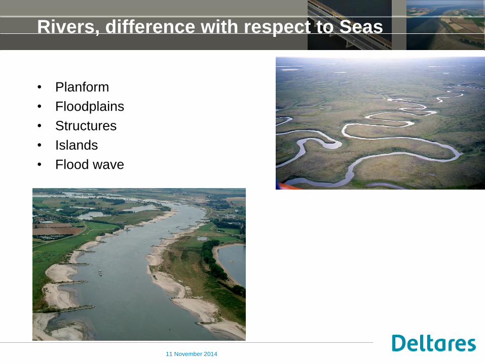
Rivers, difference with respect to Seas

• Planform

• Floodplains

• Structures

• Islands

• Flood wave

11 November 2014

Modelling – general overview good modelling practice D

efin

e m

od

elli

ng

stra

tegy

construct the model

construct grid

create topography

hydraulic structures

hydraulic model

define numerical parameters (e.g. Dt)

define physical parameters

roughness

eddy viscosity & closure model

initial condtions define boundary conditions

define outputs

morphological model

define fixed layers (sediment thickness)

define parameters

sediment size

sediment transport formula

morphological boundaries

morphological acceleration factor

other models (e.g. WAQ)

analysis absolute

comparative

Data for modelling

• Model Construction data make a model

• e.g. land boundaries, bed levels, etc.

• Boundaries (forcing) run the model

• Needed to run the model

• e.g. river discharge

• Observations confidence in the model

• Needed to calibrate and validate

• e.g. water level at stations

4

Modelling strategy

• Models to mimic reality think why!

• Models to answer a question/group of questions

• Make a strategy make your model fit for purpose

• Define area to model

• Define boundaries

• Define important processes

• Define time-scale

• Define analysis scenarios

• Make your model …

• Attention to grid construction

• Boundary conditions

• Settings

• Analyse and present results

11 November 2014

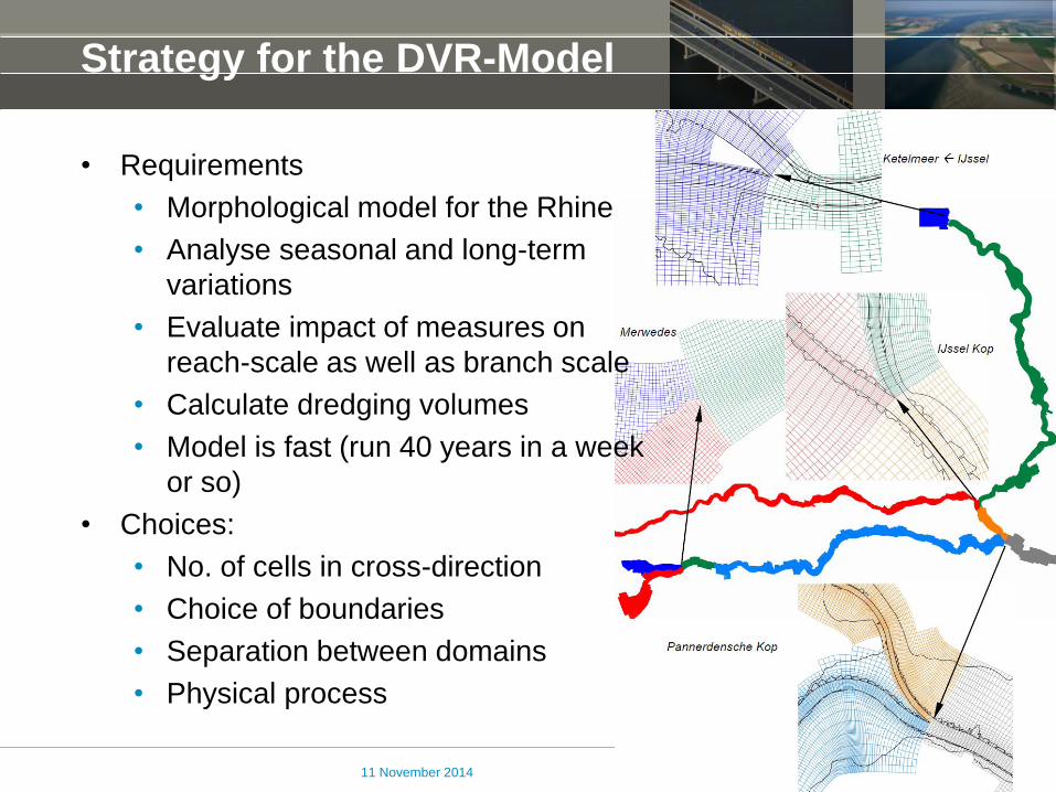
Strategy for the DVR-Model

• Requirements

• Morphological model for the Rhine

• Analyse seasonal and long-term

variations

• Evaluate impact of measures on

reach-scale as well as branch scale

• Calculate dredging volumes

• Model is fast (run 40 years in a week

or so)

• Choices:

• No. of cells in cross-direction

• Choice of boundaries

• Separation between domains

• Physical process

11 November 2014

7

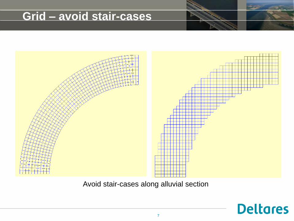
Grid – avoid stair-cases

Avoid stair-cases along alluvial section

Grid construction – bifurcation

11 November 2014

Delft3D-FLOW: Structured grid D-Flow FM: Flexible Mesh

Delft3D 4 Delft3D Flexible Mesh

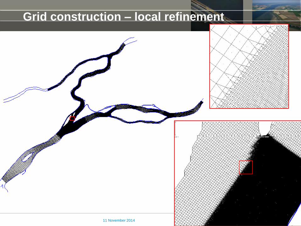
Grid construction – local refinement

11 November 2014

Grid construction – floodplains

11 November 2014

Mesh A B C D

Cells in cross-section

~ 13 8 16 32

active points 122,328 22,881 59,331 187,955

A

B

C

D

Delft3D-FLOW: structured

Delft3D-FLOW: structured

D-Flow FM

D-Flow FM

a) Delft3D-FLOW: Structured mesh

b) D-Flow FM

Number of net nodes: 331082

Number of net links: 660523

Maximum orthogonality:0.35 (poor)

General smoothness: 1 (good)

Maximum local smoothness:8 (poor)

Number of net nodes: 80860 (4.1 times less)

Number of net links: 177659 (3.7 times less)

Maximum orthohonality:0.014 (good)

General smoothness:1 (good)

Maximum local smoothness:10 (poor)

Grid construction – optimisation 1

Source: Damir Bekić et al. (Water Resources Department University of Zagreb, Croatia)

a) Structured grid (Delft3D-FLOW) does not follow the river -> requires dense mesh

b) Unstructured mesh (D-Flow FM) Follows the river -> Coarser mesh

c) D-Flow FM allows weir schematization Coarser mesh

Levees

In (a) and (b) levees and groynes are modelled within bathymetry, while in (c) mesh is more

coarse as there is no need for longitudinal elements to be covered in bathymetry

Source: Damir Bekić et al. (Water Resources Department University of Zagreb, Croatia)

Grid construction – optimisation 2

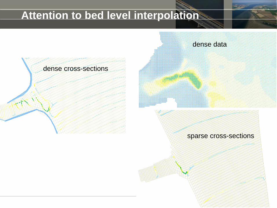
Attention to bed level interpolation

dense data

sparse cross-sections

dense cross-sections

September 7, 2012 River Flow 2012 Mohamed F.M. Yossef 14

Boundary condition: quasi-steady discharge for river morphology

0

1000

2000

3000

4000

5000

6000

7000

8000

1993 1994 1995 1996

Time

Q (

m3/s

)

0

1000

2000

3000

4000

5000

6000

7000

8000

1993 1994 1995 1996

Time

Q (

m3/s

)

Q1 Q3

Q2

0

1000

2000

3000

4000

5000

6000

7000

8000

1993 1994 1995 1996

Time

Q (m

3/s)

morfac

• Repeat a yearly schematised hydrograph using a sequence of

steady discharges

• Apply a “morphological factor” to speed up morphology (same

morphological changes in shorter flow period): factor 50 to 200

September 7, 2012 River Flow 2012 Mohamed F.M. Yossef 15

Boundary condition – discharge schematisation

0

2000

4000

6000

8000

10000

12000

14000

16000

2000 2001 2002 2003 2004 2005 2006 2007 2008 2009 2010 2011 2012 2013 2014 2015 2016 2017 2018 2019 2020 2021 2022 2023 2024 2025 2026 2027 2028 2029 2030 2031 2032 2033 2034 2035

Date

Q (

m3

/s)

11 November 2014

Boundary condition – flood attenuation

Q@x1

Q@x2

t

Q@x1

Q@x2

t

x1 = location x1 upstream

x2 = location x2 downstream

Q

Q

Dynamic simulation

QH relation at

downstream boundary

Quasi steady

Water level time-series at

downstream boundary

Parameter settings

Choice of sediment transport formula

Choice of 2D parameters

Analysis of results

2D-behaviour (40-years)

2D-behaviour (detail)

1D-behaviour (40-years)

Dune heights

Thank you

Source: Herman Kernekamp (Deltares)

Questions

11 November 2014