Drums and Bass Interlocking

i

Drums and Bass Interlocking

Pere Calopa Piedra

MASTER THESIS UPF / 2016 Master in Sound and Music Computing

Master thesis supervisors: Dr. Sergi Jordà i Dr. Perfecto Herrera

Department of Information and Communication Technologies Universitat Pompeu Fabra, Barcelona

iii

Agraïments Gràcies a tothom qui ha fet possible aquesta tesi. Agraeixo especialment als meus supervisors l’ajuda rebuda i la confiança en el meu treball. A més, m’agradaria agrair la col·laboració d’en Josep Aymí Martínez en la transcripció de un dels corpus. Tampoc m’agradaria oblidar-me de la resta de membres del grup Giant Steps i resta de membres del MTG.

v

Abstract This thesis presents the technical and theoretical details of a generative system that considers the stylistic rhythmic interaction (interlocking) between bass and drums in the context of Electronic Dance Music (EDM). The concept of rhythmic interlocking, commonly known as groove, has been vaguely studied and is still an open research field. Before designing the generative system it has been necessary to materialize a rhythmic analysis algorithm that allows to study the rhythmic interlocking between instruments. The proposed rhythmic analysis extends recent work on rhythmic similarity that computes syncopation in a rhythmic pattern based on techniques derived from rhythm perception and cognition literature. The outcome of the analysis makes possible to visualize rhythmic patterns in a low-dimensional space defined by rhythmic features relevant to groove conception (i.e. syncopation and density). In addition, we model both temporal and interlocking context of a given corpus using Markov Chains. Taking advantage of the low-dimensional “cognitive-based” representation of rhythmic patterns, the system is parametrized by global syncopation and density controls for pattern generation. The most relevant contributions of this work are the compilation of literature on the topics of groove and stylistic algorithmic composition, the comparison between different generative approaches, and the software implementation of the proposed methods for analysis, visualization and generation. Results show that our proposals are useful for stylistic modelling and give better comprehension of the problem of rhythmic interlocking. Moreover, the generative system has been implemented and partially evaluated with promising results that encourage further research on the topic. Keywords: rhythm, groove, interlocking, generative system, algorithmic composition

Index

Pg. Abstract .................................................................................................. v 1. INTRODUCTION…... ....................................................................... 1 2. STATE OF THE ART………………….…………………………… 3 2.1. Algorithmic composition ................................................................. 3 a) Algorithmic composition overview..................................................... 3 b) Interactive algorithmic composition….…………………………….. 4 c) Algorithmic composition in EDM…….……………………………. 5 d) Discussion…………………………………………………………… 6 2.2. Rhythm conceptualization ............................................................... 7 a) Interlocking and groove……………………………………………... 10 3. METHOD…………………………………………………………… 13 3.1. Dataset……………………………………………………………. 13 a) Corpus description……….................................................................. 14 3.2. Rhythm analysis………................................................................... 14 a) Representation of rhythm in a low-dimensional space....................... 18 b) Instantaneous rhythmic visualization.................................................. 19 3.3. Results……….................................................................................. 20 a) Instrument rhythmic analysis……………………………………….. 20 b) Discussion…………………………………………………………... 23 4. GENERATIVE SYSTEM BASED ON TEMPORAL AND INTERLOCKING CONTEXT………………………………………...

25

4.1. Corpus computational representation……………………………... 25 4.2. Temporal context model (TCM)………………………………….. 26 4.3. Interlocking context model (ICM)………………………………... 28 4.4. Model combination: temporal + interlocking context (TICM)...…. 29 4.5. Generation control model…………………………………………. 30 5. EVALUATION……………………………………………………… 31 5.1 Participants………………………………………………………….. 31 5.2 Design………………………………………………………………. 31 5.3 Materials…………………………………………………………….. 31 5.4 Procedure…………………………………………………………… 32 5.5 Results………………………………………………………………. 33 5.6 Discussion…………………………………………………………… 34 6. CONCLUSIONS……………………………………………………. 35 Bibliography.............................................................................................. 37 Appendix………………………………………………………………… 41

1

1. INTRODUCTION This work is inspired by the need to develop new musical tools based on how instrument rhythmic patterns interact together in a stylistic context. This thesis has been developed in the context of the Giant Steps EU Project1 (FP7-610591). The Giant Steps goals we focus on are the creation of expert systems to guide users in composition and the development of methods for music analysis in the context of Electronic Dance Music (EDM). Specifically, our interest is to model the rhythmic interaction (interlocking) between drums and bassline in the context of Electronic Dance Music. We refer as interlocking to the rhythmic interaction between simultaneous instruments to create a composite musical texture. In EDM, drums and bass are the foundation of a track. It is inconceivable an EDM track without drums and a bassline. Drums and bass conform a musical entity commonly known as Beats. Moreover, drums and bass encode most of the rhythmic information of the track. Consequently, the rhythmic interlocking between them is crucial to compose a “good Beat”. For almost thirteen years I’ve been DJing and producing different EDM styles. I thinks it is remarkable to say I haven’t formally studied music in any institution. However, together with my passion for music and technology (and specially its combination), this lack of formal musical knowledge motivated me to explore and research around “how to make good dance music”. In the EDM scene it is very common that one person composes, produces and mixes a track (in EDM, songs are called tracks). In a rock band, for instance, the process tends to be very different; someone will write the lyrics, the drummer will play a drum beat and then the bass player will start playing on top to find a nice bassline. Each member performs on his instrument according to what other members are playing, both when they are performing a pre-composed song or improvising they are constrained by stylistic rules, musical knowledge and performing expertise (e.g. play in the same key, follow a determined phrase structure, accentuate other instruments, create fills and ghost notes among others). Let’s now consider an example of an EDM producer that is making a track; the producer starts programming a drum loop, then he/she adds a bassline, then he/she plays some chords on top and he/she starts experimenting with these basic elements to create a nice danceable track. Opposed to the rock band situation, the producer needs to “know” how to “play or program” all the instruments within the track and make them work together. Even if you are a super-skilled musician, you are not always inspired, or you can get stuck looking for that “perfect” bassline, or you want to explore a new style you are not familiar, or many other situations can happen when composing music that “kill” the creative workflow. Expert systems can be a useful tool to guide users in certain parts of the composition workflow empowering creativity and inspiration. Specifically, we propose a system that guides the user in the composition of rhythmic bass patterns based on a drum-loop within a determined style. Moreover, we want the generative system to be parametrized by high-level rhythmic controls. The high-level controls manipulate syncopation and density, rhythmic features related to how we create and conceive rhythm. 1 htttp://www.giantsteps-project.eu

2

Our starting point will be the review of literature on rhythm perception and cognition to understand how rhythm is conceived within a metrical context. The idea is to take advantage of literature to materialize tools and techniques for rhythmic analysis that help to approach the comprehension of rhythmic interlocking. The methodology used to analyse the corpus extends the method proposed by Gómez-Marín for the computation of syncopation in a rhythmic pattern (Gómez-Marín et.al., 2015a, 2015b). Algorithmic composition and expert systems are not a novel trend so we will review the state of the art in this field, specifically focusing on those systems that imitate styles and those that provide user control in the generative process. Proposed analysis and generation algorithms in this thesis are implemented in prototype software tools using Max2 and Python3 programming languages.

2 http://www.cycling74.com/products/max 3 http://www.python.org

3

2. STATE OF THE ART 2.1 Algorithmic composition As we will see throughout this section, composing music using algorithmic techniques is not a recent trend, so we will briefly make a historical chronology. This section will start briefly explaining the origins of algorithmic compositions using computers and the usage of Markov Chains (MC) for stylistic modelling. After presenting some of the pioneer approaches to Algorithmic Composition we will review two current approaches for stylistic Algorithmic Composition. First, interactive generative systems based on MC. Then, EDM generative systems that generate full-tracks based on a pre-analysed stylistic corpus. a) Algorithmic composition overview Algorithmic composition (AC) is not a recent research topic and has been quite broadly explored. By algorithmic composition we will refer to the computational implementation of algorithms to compose music. Previous to the existence of computers, musicians already used algorithms to compose music (e.g. Mozart, Cage), and these could obviously also be implemented with computers. We must difference between using algorithms to compose a complete music piece and using algorithms to provide support to the user during the composition or performance of music. This thesis will focus in the former approach, also known as computer-aided algorithmic composition (CAAC) or expert user-agents. CAAC area keeps active either for research or commercial software development (e.g. graphical tools, programming languages, software plugins) (Fernández and Vico, 2013). This review of the state of the art will only take advantage of open-knowledge, as commercial algorithms are less accessible. Literature related to algorithmic composition relies in a broad set of areas going from art to computational engineering. This sparse location of the information makes difficult to take into account previous achievements, which causes many authors to “reinvent the wheel” (Fernández and Vico, 2013). This fact makes very relevant to build a scheme relating previous work on the topic of interest. Fernandez and Vico in 2013 published a survey about the Artificial Intelligence (AI) methods used in algorithmic composition (Fernández and Vico, 2013). The survey by Fernández and Vico captures the state of the art in 2013 and older approaches grouped depending on the methods used. Since AC is an ‘old’ trend it’s interesting to review the most relevant historical approaches focusing on those using Markov models for stylistic AC. As algorithmic composition relies on computers, the technologies available become a key constraint. Earliest use of computers to compose music dates back in mid-1950, concurring with the concept of AI. In those times, computers were expensive, slow and more important, difficult to use. If we compare with the current technological context, we realise that the conditions have completely turned around; now technology is not a key constraint anymore. The most cited example of early algorithmic composition is Hiller and Isaacson’s (1958) Illiac Suite, a composition generated using rule systems and Markov chains in 1956. This work inspired in the next decade an experimentation environment that resulted in standard implementations of the various methods used by Hiller and others. Another early relevant example is Iannis Xenakis, that used stochastic

4

approaches within computers since early 60s, being a pioneer (Ames, 1989). Charles Ames reviews AC between 1956 and 1986, also covering other less-cited approaches (Ames, 1989). Previous cited works rely on custom programmed stochastic models, where probabilities and rules were manually implemented. A less known work, Push Button Bertha (1956), by mathematicians Martin Klein and Douglas Bolitho at Burroughs Corporation, sets the historical starting point for the idea this thesis is based on. In this work the song was composed using a previously analysed corpus to set the rules of the generation system automatically. The methods implied where based on Markov Chain and Charles Ames explain them in his AC review (Ames, 1989). Markov Chains in AC research are based on probability matrices that establish the transition between musical objects (e.g. notes, chords, music sections…). As commented before, we will focus on those models using a pre-analysed corpus. A limitation of Markov Chains that soon became apparent is that they can only model local statistical similarities. Models using high order chains tend to replicate the corpus while low order ones produce strange and unmusical compositions (Moorer, 1972). Literature reviews show (Ames, 2011) how the combination between Markov models and other techniques produce better results than using them on its own. After considering this ‘classical’ literature we are going to focus on recent work that inspires our system. Between the classical reviewed systems and the ones presented in next sections there is a remarkable time gap of almost 30 years. Markov-based systems in this gap are variations of the reviewed classical systems, and don’t represent relevant milestones in stylistic AC. Most of the Markov-based systems are combined with other techniques (e.g. fitness functions, Petri nets, grammar hierarchies among others) most focusing on melody generation (North, 1991; Lyon, 1995; Werner and Todd, 1997). However, Ames and Domino presented the Cybernetic Composer that models rhythmic patterns in Jazz and Rock using Markov Chains (Ames and Domino, 1992). b) Interactive algorithmic composition

François Pachet published The Continuator (Pachet, 2002) in 2002. The system proposed is novel in the way it combines interactive musical systems and imitation systems, which are not interactive. The system is based on a variable-order Markov model extracted from MIDI data, with the possibility of managing in real-time musical issues such as rhythm, harmony or imprecision. The input MIDI notes sequences generate a prefix tree to build the transition probabilities between notes. The tree model is used to allow a variable-length Markovian process to create continuations based on a target sequence. The system allows polyphony in the sense that it allows chords, but not different instruments. To handle the rhythmic pattern generation, the author used four different modes to choose from. The first refers to ‘natural rhythm’ as it replicates the temporal structure used in the training process. The second mode is ‘linear rhythm’, generating a note every 8th note measure given a specified tempo. The third mode is to replicate the rhythm of a real-time input phrase. This mode allows creating rhythmically similar sequences. Last mode, ‘fixed metrical structure’, is to use a metrical structure, quantizing the generation process. The novelty of this work is to design a tractable system with stylistic consistency with satisfying results.

5

Later work by Pachet et al. (Pachet, Roy and Barbieri, 2011) go further in the evolution of Markov processes and presents a mathematical framework for using finite-order Markov models with control constraints. The described process allows the user to constrain the generation in real-time, e.g. melodic contour, keeping the initial statistical distribution. This is not possible using only MC, as control constraints induce long-term dependencies that can’t be handled without violating the Markov hypothesis of limited memory (Pachet, Roy and Barbieri, 2011). Generating sequences by a simple random walk algorithm and applying control constraints in real-time, can yield undesirable consequences. For instance, the so-called zero-frequency problem occurs when an item with no continuation is chosen (Pachet, Roy and Barbieri, 2011).

Most approaches before Pachet et al. (Pachet, Roy and Barbieri, 2011) proposed heuristic search solutions to solve the constraint related issues (e.g. case-based reasoning generate-and-test (Dubnov et al., 2003)). Heuristic approaches do not offer any guarantee to find a solution, and are not consistent with the initial probabilities or are computationally expensive. Pachet et al. propose a more efficient approach to handle Markov models and constraints; to generate a new model that combined with constraints is still, probability-wise, equivalent to the initial Markov model. Authors show that when control constraints remain within the Markov scope, not violating Markov hypothesis, a model can be created with a low complexity (Pachet, Roy and Barbieri, 2011). The algorithm is based on arc-consistency and renormalization. This ensures that any choice made during the generation process by a random walk will lead to a sequence, without search. Moreover, the resulting sequence will satisfy the constraints and the initial Markov model. Authors apply this method to create, given a target sequence, musically valid continuations, variations or answers, setting the appropriate restrictions given a stylistic knowledge (e.g. jazz scales). This approach was tested with users getting control over the generation constraints using gesture sensors for real-time generation. c) Algorithmic composition in EDM

In 2013, Eigenfeldt and Pasquier published a set of papers in the context of a generative system based on style (Eigenfeldt and Pasquier, 2013; Andersson, Eigenfeldt and Pasquier, 2013). Their first system, called GESMI (Generative Electronica Statistical Modelling Instrument), generates EDM tracks through corpus modelling using Markov models. Their idea was to create an autonomous system able to play in an event resulting artistically satisfying for the audience (Eigenfeldt and Pasquier, 2013). In the context of their research they manually-annotated a corpus containing transcriptions for four genres: Breaks, House, Dubstep and Drum and Bass. Authors do also consider aspects like form that are not in the scope of our thesis.

The interesting fact of their approach is that they consider both the horizontal context (i.e. time) and the vertical one (i.e. polyphony, different instruments). For this purpose, they use Pachet et al. method (Pachet, Roy and Barbieri, 2011) (see previous paragraph). In contrast to Pachet, the authors are not interested in preserving the initial

6

model probabilities for the sake of variety and surprise (Eigenfeldt and Pasquier, 2013). Their system use MC for temporal dependencies and vertical dependencies. The vertical dependency between the instruments (interlocking), takes the drum patterns generated as reference. In their generation algorithm is generated first the drum pattern, and then the other instruments based on their concurrency.

Drum patterns consist of 4 different instruments (i.e. Kick, Snare, Closed Hihat, Open Hihat). Patterns are generated using three different methods; zero and first-order Markov on individual instruments and first-order Markov on combined instruments. Their patterns are generated within a sixteenth-note resolution for each beat measure, resulting in four onsets per beat. Authors point that EDM rarely, if ever, ventures outside of sixteenth-note subdivisions per beat (Eigenfeldt and Pasquier, 2013).

For Bassline generation they designed a two-step process, based on determining the onsets and overlaying the pitches. Bassline onsets are represented by three states: note onset, held note and rests. The bassline patterns are determined based on the concurrency with the drums and the overlaid pitch using different transition matrices. The system adds different constraints for bassline generation that will be combined with the Markov models. Those constraints are: density (i.e. number of onsets), straightness (i.e. favour or not syncopation), dryness (i.e. favour held versus rests notes), jaggedness (i.e. favour greater or lesser differentiation between consecutive pitch classes). Authors discuss that, by targeting different parameters, it is possible to create divergent results within a same style in long performances but not how they are applied in the generation process (Eigenfeldt and Pasquier, 2013).

The second system in the same context of research involved the same authors and Christopher Anderson (Anderson, Eigenfeldt and Pasquier, 2013). It is called GEDMAS (Generative Electronic Dance Music Algorithmic System) and is like GESMI. It is implemented in Max and integrated in Live. In further publications, the authors added Genetic Algorithms (GA) to increase the variability of the system while combining them with the analysed dataset of an EDM style. It is relevant to point that authors used a manually annotated dataset instead of using Signal Processing techniques to transcribe the instances of the dataset because of its difficulty.

d) Discussion

Most systems for stylistic algorithmic composition use processes based on Markov Chains to build a statistical model of the seed corpus. Previous approaches of EDM generation have already considered the interlocking between bass and drums (Eigenfeldt and Pasquier, 2013; Andersson, Eigenfeldt and Pasquier, 2013). The later, approach the generation of stylistic full-tracks based on a pre-analysed corpus (Andersson, Eigenfeldt and Pasquier, 2013). While their system is able to play for hours as a standalone system, we are interested in a tool that can guide the musician during the composition. Opposite to a parametrized standalone system, we are interested in providing musically meaningful controls to the user. Other approaches have already defined generative models with real-time controls (Pachet, 2002), but they tend not consider style in the sense of a corpus, using a MIDI keyboard real-time input instead, and neither the interaction between instruments.

7

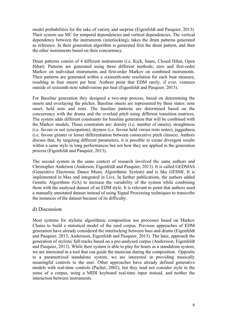
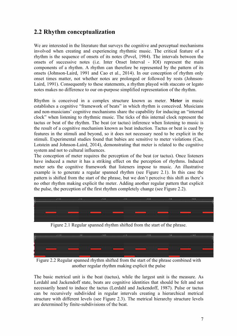
2.2 Rhythm conceptualization We are interested in the literature that surveys the cognitive and perceptual mechanisms involved when creating and experiencing rhythmic music. The critical feature of a rhythm is the sequence of onsets of its notes (Povel, 1984). The intervals between the onsets of successive notes (i.e. Inter Onset Interval - IOI) represent the main components of a rhythm. A rhythm can therefore be represented by the pattern of its onsets (Johnson-Laird, 1991 and Cao et al., 2014). In our conception of rhythm only onset times matter, not whether notes are prolonged or followed by rests (Johnson-Laird, 1991). Consequently to these statements, a rhythm played with staccato or legato notes makes no difference to our on-purpose simplified representation of the rhythm. Rhythm is conceived in a complex structure known as meter. Meter in music establishes a cognitive “framework of beats” in which rhythm is conceived. Musicians and non-musicians’ cognitive mechanisms share the capability for inducing an “internal clock” when listening to rhythmic music. The ticks of this internal clock represent the tactus or beat of the rhythm. The beat (or tactus) inference when listening to music is the result of a cognitive mechanism known as beat induction. Tactus or beat is cued by features in the stimuli and beyond, so it does not necessary need to be explicit in the stimuli. Experimental studies found that babies are sensitive to meter violations (Cao, Lotstein and Johnson-Laird, 2014), demonstrating that meter is related to the cognitive system and not to cultural influences. The conception of meter requires the perception of the beat (or tactus). Once listeners have induced a meter it has a striking effect on the perception of rhythms. Induced meter sets the cognitive framework that listeners impose to music. An illustrative example is to generate a regular spanned rhythm (see Figure 2.1). In this case the pattern is shifted from the start of the phrase, but we don’t perceive this shift as there’s no other rhythm making explicit the meter. Adding another regular pattern that explicit the pulse, the perception of the first rhythm completely change (see Figure 2.2).

Figure 2.1 Regular spanned rhythm shifted from the start of the phrase.

Figure 2.2 Regular spanned rhythm shifted from the start of the phrase combined with another regular rhythm making explicit the pulse

The basic metrical unit is the beat (tactus), while the largest unit is the measure. As Lerdahl and Jackendoff state, beats are cognitive identities that should be felt and not necessarily heard to induce the tactus (Lerdahl and Jackendoff, 1987). Pulse or tactus can be recursively subdivided in regular intervals creating a hierarchical metrical structure with different levels (see Figure 2.3). The metrical hierarchy structure levels are determined by finite-subdivisions of the beat.

8

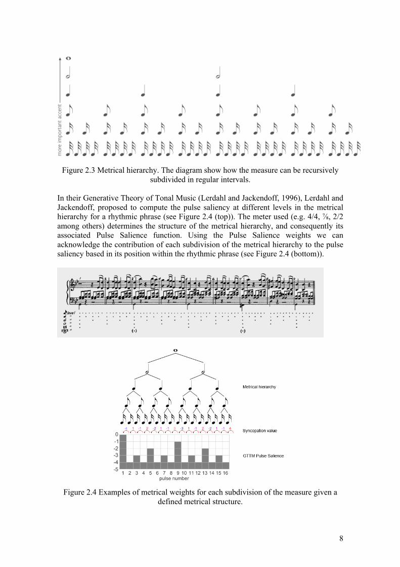
Figure 2.3 Metrical hierarchy. The diagram show how the measure can be recursively subdivided in regular intervals.

In their Generative Theory of Tonal Music (Lerdahl and Jackendoff, 1996), Lerdahl and Jackendoff, proposed to compute the pulse saliency at different levels in the metrical hierarchy for a rhythmic phrase (see Figure 2.4 (top)). The meter used (e.g. 4/4, ⅞, 2/2 among others) determines the structure of the metrical hierarchy, and consequently its associated Pulse Salience function. Using the Pulse Salience weights we can acknowledge the contribution of each subdivision of the metrical hierarchy to the pulse saliency based in its position within the rhythmic phrase (see Figure 2.4 (bottom)).

Figure 2.4 Examples of metrical weights for each subdivision of the measure given a

defined metrical structure.

9

In a metrical context, notes with onsets on units of metrical importance will reinforce the meter perception, while those with onsets in units with “less” metrical importance will disturb the meter (Volk, 2008). This phenomena of meter disturbance is known as syncopation. Opposite to Volk, Temperley argues that some kinds of syncopation actually reinforce the meter rather than disturbing it (Butler, 2006). Syncopation is a fundamental rhythmic property “manipulated” by musicians and is completely dependent on the conception of meter. Without meter the perception of syncopation is not possible. The perceptions of rhythm and meter are mutually interdependent. The cognitive system infers meter from a rhythm, but the nature of the rhythm itself depends on the meter (Essens, 1995). According to Johnson-Laird: “different rhythms vary in the degree to which they resemble one another” (Johnson-Laird, 1991). Some rhythms tend to be perceived as similar while others are clearly perceived as different. Johnson-Laird states that rhythms are perceived and created under cognitive prototypes. The different prototype rhythms are distinguished by its pattern of onsets. All patterns of onsets that belong to the same underlying prototype are grouped under the same rhythmic family. Rhythmic families are determined by the theory of rhythmic families initially proposed by Johnson-Laird (Johnson-Laird, 1991) and extended by Cao, Lotstein and Johnson-Laird (Cao, Lotstein and Johnson-Laird, 2014). The theory of rhythmic families by Cao, Lotstein and Johnson-Laird stipulates that there are only three types of musical events that matter with respect to the meter (Cao, Lotstein and Johnson-Laird, 2014). By order of importance we can find the following categories:

• Syncopations (S) • Notes on the beat (N) • Other like rests or ties (O)

Each beat in any metrical rhythm can be categorized as an instance of one, and only one, of the three categories. This way we can represent a rhythm based on the category of each beat conforming the phrase. The family theory makes five principal predictions (Cao, Lotstein and Johnson-Laird, 2014):

• If two rhythms share the same pattern of onsets, then they should tend to be judged similar.

• If two rhythms are from the same family, with other parameters being equal, they should be judged as more similar than two rhythms from different families.

• If individuals try to reproduce a rhythm, their errors should tend to yield rhythms in the same family as the original target as opposed to rhythms in a different family.

• Errors in reproduction should be more likely to occur in the case of syncopation. • The fewer the notes in a rhythm, the easier it should be to be reproduced.

Recently Gómez-Marín proposed a new family categorization extending the theory of rhythmic families by Cao, Lotstein and Johnson-Laird (Gómez-Marín et.al., 2015a, 2015b). Instead of considering the three categories previously proposed, Gómez-Marín method discriminates between 3 types of syncopation, 3 types of reinforcement and a

10

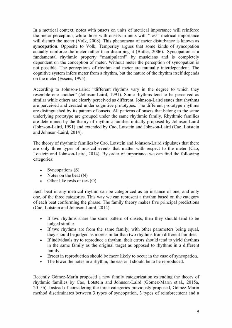
category that mixes reinforcement and syncopation, preserving the category for other events. The categorization now clusters all possible beat patterns in 8 rhythmic families (see Table 2.1).

Table 2.1. Relation between syncopation group (rhythmic family), syncopation value and beat patterns. Symbol ‘x’ denote the presence of an onset in the next beat while

symbol ‘_’ denotes its absence.

a) Interlocking and groove We refer as rhythmic interlocking to the interaction between simultaneous rhythms for creating a composite one. In the context of Dance Music (e.g. House, Techno, Soul, African music among others), rhythmic patterns are presented in a repetitive pattern exploiting the cyclical nature of rhythm. As music is conceived in cycles within a metrical context, it is possible to create systematic rhythmic variations to induce body motion (i.e. dance) and musical interest to the whole music piece. The interlocking between bass and drums in EDM has been vaguely studied (Butler, 2006). However, interlocking in Dance Music is commonly known as groove. In literature, groove has been studied and operationally defined as “the property of rhythm that induce wanting to move a part of the body “(Madison, 2006). It’s important to emphasize that we are referring to a psychological experience dependent on the listener. Groove in Dance Music is also a common word to describe a good danceable rhythm (Butler, 2006). Groove can be induced both by a monotimbral pattern or by a complex rhythmic texture. In monophonic rhythms, experimental studies reveal a relationship between groove and rhythmic features (Holm and Isaksson, 2010 and Madison, 2014). Authors asked musicians to create a groovier version and a less groovy version of a given target monophonic melody, while preserving similarity to the target. Results showed a positive correlation between syncopation and density when creating groovier performances. That means that musicians tend to add syncopated notes when creating groovy variations of a monophonic melody (Holm and Isaksson, 2010 and Madison, 2014). While this is a good starting point, the combination between syncopation and density for inducing groove is still not clear. However, in an EDM track, we find multiple rhythmic layers that we perceive blended together into a composite entity known as beats. Literature focused on groove in EDM determines that the perception of the composite rhythm is something more than just the sum of the independent layers (Butler, 2006; Holm and Isaksson, 2010). Each of the

11

individual instruments is part of a network of interrelated patterns, what we call rhythmic interlocking. According to Holm and Isaakson: “groove may not be solely explained as specific parts of the music, but is something that comes out of the picture, the sum is more than all the parts” (Holm and Isaksson, 2010). While an independent rhythm can be perceived as highly syncopated, the composite rhythm tends to reinforce the meter when listened together with the other elements (Butler, 2006).

13

3. METHOD The main objectives to be developed are, first to define and implement a rhythmic analysis methodology to model rhythm interlocking in a stylistic corpus, materializing existing literature on rhythmic perception and cognition. Second, to develop tools for visualization of rhythmic interlocking in a low-dimensional space. Third, to develop a generative system, based on the proposed analysis, that will be able to create basslines and drums loops stylistically-consistent with the user controls on syncopation and density. We start by discussing the corpus creation process and its requirements. We follow up detailing the proposed methodology, and we conclude explaining both the software implementation and its fundamental concepts. Our interest is to build a model being able to characterize the rhythmic properties of a certain musical style. Onsets are the critical feature of rhythm perception and cognition, so we are only interested in the binary representation of onsets of bass and drums instruments. 3.1 Dataset The most straightforward approach is to extract symbolic information from MIDI files (i.e. using ‘Note On’ events). We can find a considerable amount of MIDI collections of drums and bass patterns in Internet, but they are either found in different collections (stylistically inconsistent) or the files are not matched (it is not possible to extract interlocking information between instruments). Another issue retrieving data directly from MIDI files is that they are a score-like representation, we need to synthesize them to listen them, so it becomes difficult to evaluate its quality and style. We need a corpus of tracks stylistically consistent that contain matched bass and drums MIDI-like files. To ensure the stylistic consistency we decided to manually select audio tracks composed by the same artist, chosen because of its idiomatic style. The selected artists are the German duet Booka Shade4 and the British DJ and producer Mr.Scruff5. Booka Shade are founders of Get Physical, one of the most successful EDM labels. Their music is mainly based on melodic basslines and synths supported by electronic drum beats. Mr.Scruff is well-known for his marathon DJ sessions exploiting his eclectic style. As a producer he released albums and single EPs with Ninja Tune6, one of the most important independent music record labels. As both the bass and drums are main instruments in both styles, we can attempt to decode the rhythmic relationship between them by capturing the Booka Shade-ish style and the Mr.Scruff-ish style. Decoding bass and drums patterns from an audio signal requires processing the audio tracks to represent the rhythmic information in a symbolic representation. This process is known as “transcription”, and its automation it's an ongoing research in the MIR community (Goto, 2004; Salamon and Gomez, 2009; Salamon, 2013). The case of automatically transcribing a monotimbral audio signal can be achieved with accuracy (de Chevigné and Kawahara, 2002). But, when trying to transcribe different instruments

4 htttp://www.bookashade.com 5 http://www.mrscruff.com 6 http://www.ninjatune.net

14

from a mixed and mastered audio track the problem becomes much more difficult. The complexity of the transcription relies on the source separation process required. Moreover, in EDM production it is very common to “glue” the different instruments using analog or DSP techniques (e.g. compression, EQ), which makes transcription even more difficult. a) Corpus description The first corpus is conformed by 23 audio tracks by Booka Shade, manually selected from its discography. The second is conformed by 24 audio tracks by Mr.Scruff also manually selected. The selection was made based on the stylistic consistency of the tracks within each corpus. We are only interested in the main section of each of the tracks, all 8-bars long. According to literature, 8 bars is a common measure for sections in EDM (Butler, 2006). This decision was taken to avoid retrieving structural-independent information. So the corpus is stylistically consistent and, moreover, it refers to musical phrases with the same musical intention. The audio tracks need to be transcribed to obtain separate bassline and drums symbolic representations (e.g. MIDI tracks). After exploring different automatic transcription methods (such as Ableton Live7 tools and Essentia8 using MELODIA9 for bass transcription, see Appendix) we decided to build the corpus using manual transcription aided by some semi-automatic tools such as Celemony’s Melodyne10. Transcriptions were exported as MIDI files, quantized to a 1/16 bars resolution grid. The process is time-consuming and not scalable, so automatic transcription tools and sound sources need to be further improved. The use of STEMS11, as Native Instruments is promoting, could be an alternative strategy in the future . 3.2 Rhythm analysis In this section we extend previous computational approaches to measure syncopation of a rhythm in a metrical context. We use the method recently proposed by (Gómez-Marín et.al., 2015a, 2015b) and used for rhythmic similarity, extending the “family theory” proposed by (Johnson-Laird, 1991) and later by (Cao, Lotstein and Johnson-Laird, 2014). Instead of using Gòmez-Marín’s methodology to measure rhythmic similarity, we propose a generalisation of the method to obtain a cognitive-based representation of rhythm. This method assigns a syncopation value to a beat pattern, based on a beat profile to later cluster all possible beat onset patterns into 8 rhythmic families (Gómez-Marín et.al., 2015a, 2015b). In addition to Gómez-Marín’s method, we propose to compute the

7 https://www.ableton.com/en/live/ 8 http://essentia.upf.edu/ 9 http://mtg.upf.edu/technologies/melodia 10 http://www.celemony.com/en/melodyne/what-is-melodyne 11 ttps://www.native-instruments.com/es/specials/stems/

15

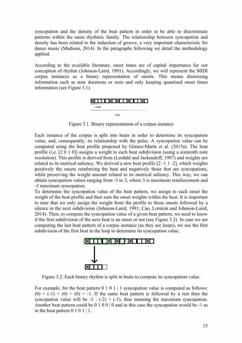
syncopation and the density of the beat pattern in order to be able to discriminate patterns within the same rhythmic family. The relationship between syncopation and density has been related to the induction of groove, a very important characteristic for dance music (Madison, 2014). In the paragraphs following we detail the methodology applied. According to the available literature, onset times are of capital importance for our conception of rhythm (Johnson-Laird, 1991). Accordingly, we will represent the MIDI corpus instances as a binary representation of onsets. This means dismissing information such as note durations or rests and only keeping quantized onset times information (see Figure 3.1).

Figure 3.1. Binary representation of a corpus instance

Each instance of the corpus is split into beats in order to determine its syncopation value, and, consequently, its relationship with the pulse. A syncopation value can be computed using the beat profile proposed by Gòmez-Marín et al. (2015a). The beat profile (i.e. [2 0 1 0]) assigns a weight to each beat subdivision (using a sixteenth note resolution). This profile is derived from (Lerdahl and Jackendoff, 1987) and weights are related to its metrical saliency. We derived a new beat profile [2 -1 1 -2], which weights positively the onsets reinforcing the beat and negatively those that are syncopations, while preserving the weight amount related to its metrical saliency. This way, we can obtain syncopation values ranging from -3 to 3, where 3 is maximum reinforcement and -3 maximum syncopation. To determine the syncopation value of the beat pattern, we assign to each onset the weight of the beat profile and then sum the onset weights within the beat. It is important to note that we only assign the weight from the profile to those onsets followed by a silence in the next subdivision (Johnson-Laird, 1991; Cao, Lotstein and Johnson-Laird, 2014). Then, to compute the syncopation value of a given beat pattern, we need to know if the first subdivision of the next beat is an onset or not (see Figure 3.2). In case we are computing the last beat pattern of a corpus instance (as they are loops), we use the first subdivision of the first beat in the loop to determine its syncopation value.

Figure 3.2. Each binary rhythm is split in beats to compute its syncopation value.

For example, for the beat pattern 0 1 0 1 | 1 syncopation value is computed as follows: (0) + (-1) + (0) + (0) = -1. If the same beat pattern is followed by a rest then the syncopation value will be -3 : (-2) + (-1), thus meaning the maximum syncopation. Another beat pattern could be 0 1 0 0 | 0 and in this case the syncopation would be -1 as in the beat pattern 0 1 0 1 | 1.

16

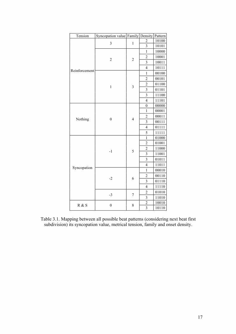
Beat patterns sharing the same syncopation values are clustered into the same rhythmic family. Gómez-Marín proposes this method to cluster beat patterns, thus extending the family theory. The main idea behind this clustering is that “families of rhythms” are cognitive prototypes. That means that beat patterns within the same family are more similar between them than with beat patterns belonging to other “families”, as they are created and perceived as the same cognitive prototype (Johnson-Laird, 1994; Cao et al., 2014). Reinforcement(R) and syncopation(S) families are split in three categories respectively. A new family is added considering reinforcement and syncopation (R & S), while preserving a family for patterns not relevant to the meter (N). Beat patterns within R&S and N families have a syncopation value of 0, but the combination of reinforcement and syncopation in the same beat, should be considered as a special case (Gómez-Marín et.al., 2015a, 2015b). Given this methodology, we can categorize all possible beat patterns into 8 groups. Those groups represent cognitive prototypes. Beat patterns within the same group share the same syncopation value. Moreover, we can compute the onset density of the patterns. (see Table 3.1).

17

Tension Syncopation value Family Density Pattern

Reinforcement

3 1 2 10100 3 10101

2 2

1 10000 2 10001 3 10011 4 10111

1 3

1 00100 2 00101 2 01100 3 01101 3 11100 4 11101

Nothing 0 4

0 00000 1 00001 2 00011 3 00111 4 01111 5 11111

Syncopation

-1 5

1 01000 2 01001 2 11000 3 11001 3 01011 4 11011

-2 6

1 00010 2 00110 3 01110 4 11110

-3 7 2 01010 3 11010

R & S 0 8 2 10010 3 10110

Table 3.1. Mapping between all possible beat patterns (considering next beat first

subdivision) its syncopation value, metrical tension, family and onset density.

18

a) Representation of rhythm in a low-dimensional space The proposed rhythm analysis extracts syncopation values and density of each beat, and is used to represent rhythmic patterns in a low-dimensional geometrical space. As we are interested in the study of rhythmic relationships between bass and drums, we propose a rhythmic space in which different instruments rhythmic representations can be studied together. This rhythmic relationship, which we will call interlocking, is fundamental in EDM and is commonly known as groove. Experiments showed that when asked to increase or decrease groove to a target rhythm pattern, musicians do mostly alter syncopation and density (Holm and Isaksson, 2010). More specifically, when asked to add groove, musicians incremented the syncopation and the density of the rhythmic pattern. In the case of performing the pattern with less groove, results were not that clear, but musicians predominantly decreased syncopation and density. These experiments were carried out using monophonic melodies. When considering groove in polyphonic rhythms we refer to the perception of the textural layers created by the mix of the rhythmic elements (Butler, 2006). Literature referring to groove in EDM states that each of the drum instruments within a polyphonic drum pattern has a specific “rhythm function”. For instance, in styles like Techno, House or Trance, the Kick drum makes explicit the meter, while hi-hats are played in a lower metrical hierarchy (e.g. 1/8th or 1/16th notes). Applying the proposed rhythmic analysis to each of the instruments within a corpus track, we can analyse their rhythmic properties and how they interact. We propose a rhythmic space where beat patterns are mapped to a discrete 2D space by a non-bijective mapping. The dimensions of the space are determined by the syncopation and density values. As previously stated, the relationship between syncopation and density is not formally defined, so we will consider them as orthogonal and independent dimensions (see Figure 3.3). A beat pattern can then be located in this space, according to its syncopation value and density. It is important to point out that the non-bijective mapping arises from the fact that there can be more than one pattern with the same syncopation and density values (e.g. beat patterns 0100|1 and 1100|0 have syncopation value -1 and density is 2). The non-bijectivity of the mapping function makes not possible to use this space for directly generating stylistic rhythmic patterns, but it can be useful for visualization applications.

Figure 3.3. Beat patterns mapping in the Rhythmic Space

19

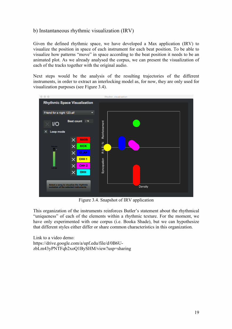
b) Instantaneous rhythmic visualization (IRV) Given the defined rhythmic space, we have developed a Max application (IRV) to visualize the position in space of each instrument for each beat position. To be able to visualize how patterns “move” in space according to the beat position it needs to be an animated plot. As we already analysed the corpus, we can present the visualization of each of the tracks together with the original audio. Next steps would be the analysis of the resulting trajectories of the different instruments, in order to extract an interlocking model as, for now, they are only used for visualization purposes (see Figure 3.4).

Figure 3.4. Snapshot of IRV application

This organization of the instruments reinforces Butler’s statement about the rhythmical “uniqueness” of each of the elements within a rhythmic texture. For the moment, we have only experimented with one corpus (i.e. Booka Shade), but we can hypothesize that different styles either differ or share common characteristics in this organization. Link to a video demo: https://drive.google.com/a/upf.edu/file/d/0B6U-zbLm43yPNTFqb2xoQ1BySHM/view?usp=sharing

20

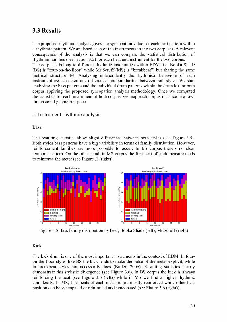
3.3 Results The proposed rhythmic analysis gives the syncopation value for each beat pattern within a rhythmic pattern. We analysed each of the instruments in the two corpuses. A relevant consequence of the analysis is that we can compare the statistical distribution of rhythmic families (see section 3.2) for each beat and instrument for the two corpus. The corpuses belong to different rhythmic taxonomies within EDM (i.e. Booka Shade (BS) is “four-on-the-floor” while Mr.Scruff (MS) is “breakbeat”) but sharing the same metrical structure 4/4. Analysing independently the rhythmical behaviour of each instrument we can determine differences and similarities between both styles. We start analysing the bass patterns and the individual drum patterns within the drum kit for both corpus applying the proposed syncopation analysis methodology. Once we computed the statistics for each instrument of both corpus, we map each corpus instance in a low-dimensional geometric space. a) Instrument rhythmic analysis Bass: The resulting statistics show slight differences between both styles (see Figure 3.5). Both styles bass patterns have a big variability in terms of family distribution. However, reinforcement families are more probable to occur. In BS corpus there’s no clear temporal pattern. On the other hand, in MS corpus the first beat of each measure tends to reinforce the meter (see Figure .1 (right)).

Figure 3.5 Bass family distribution by beat; Booka Shade (left), Mr.Scruff (right)

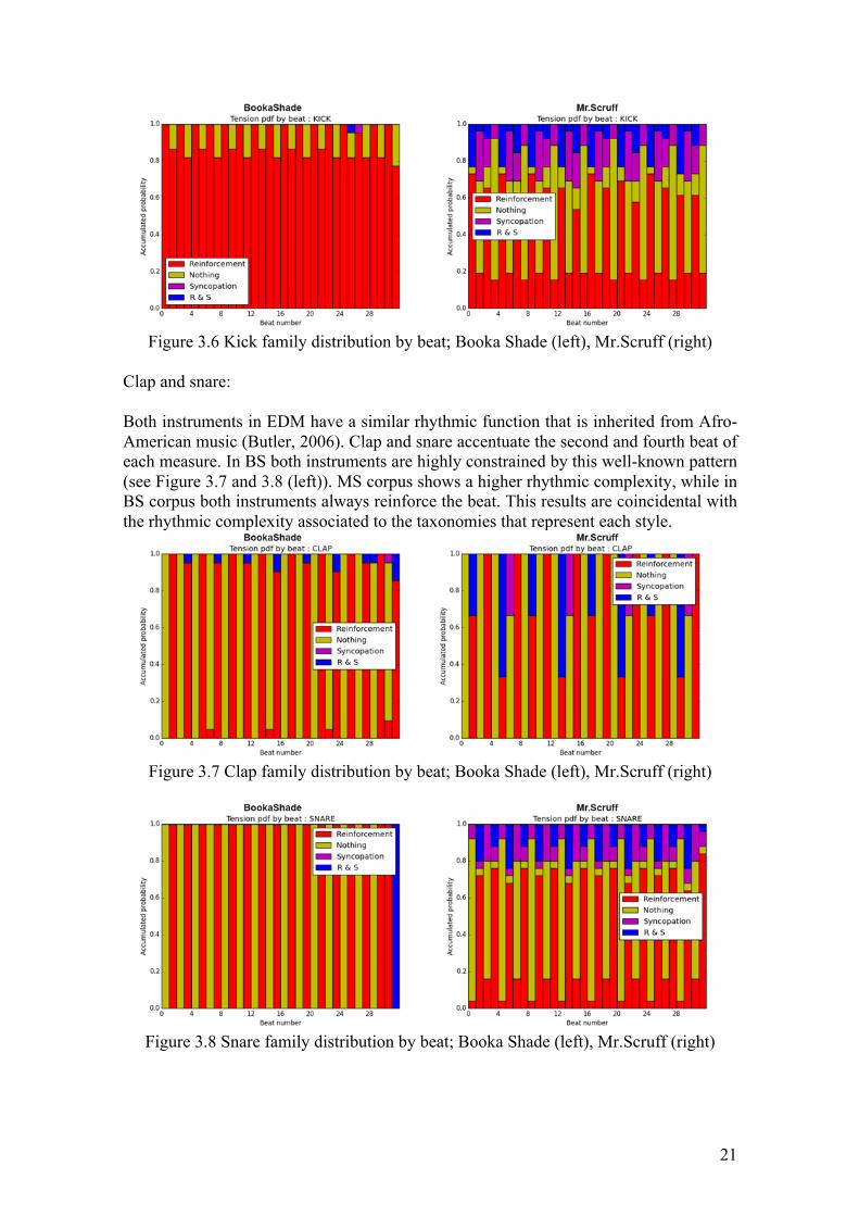
Kick: The kick drum is one of the most important instruments in the context of EDM. In four-on-the-floor styles like BS the kick tends to make the pulse of the meter explicit, while in breakbeat styles not necessarily does (Butler, 2006). Resulting statistics clearly demonstrate this stylistic divergence (see Figure 3.6). In BS corpus the kick is always reinforcing the beat (see Figure 3.6 (left)) while in MS we find a higher rhythmic complexity. In MS, first beats of each measure are mostly reinforced while other beat position can be syncopated or reinforced and syncopated (see Figure 3.6 (right)).

21

Figure 3.6 Kick family distribution by beat; Booka Shade (left), Mr.Scruff (right)

Clap and snare: Both instruments in EDM have a similar rhythmic function that is inherited from Afro-American music (Butler, 2006). Clap and snare accentuate the second and fourth beat of each measure. In BS both instruments are highly constrained by this well-known pattern (see Figure 3.7 and 3.8 (left)). MS corpus shows a higher rhythmic complexity, while in BS corpus both instruments always reinforce the beat. This results are coincidental with the rhythmic complexity associated to the taxonomies that represent each style.

Figure 3.7 Clap family distribution by beat; Booka Shade (left), Mr.Scruff (right)

Figure 3.8 Snare family distribution by beat; Booka Shade (left), Mr.Scruff (right)

22

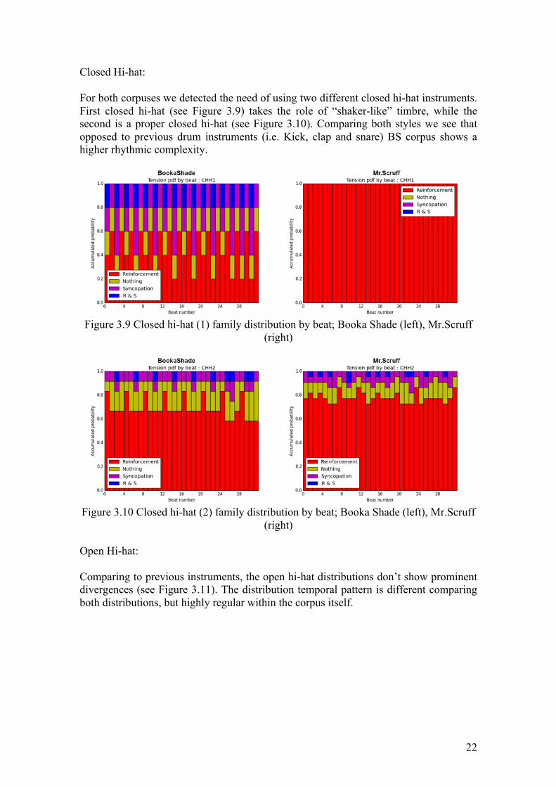
Closed Hi-hat: For both corpuses we detected the need of using two different closed hi-hat instruments. First closed hi-hat (see Figure 3.9) takes the role of “shaker-like” timbre, while the second is a proper closed hi-hat (see Figure 3.10). Comparing both styles we see that opposed to previous drum instruments (i.e. Kick, clap and snare) BS corpus shows a higher rhythmic complexity.

Figure 3.9 Closed hi-hat (1) family distribution by beat; Booka Shade (left), Mr.Scruff

(right)

Figure 3.10 Closed hi-hat (2) family distribution by beat; Booka Shade (left), Mr.Scruff

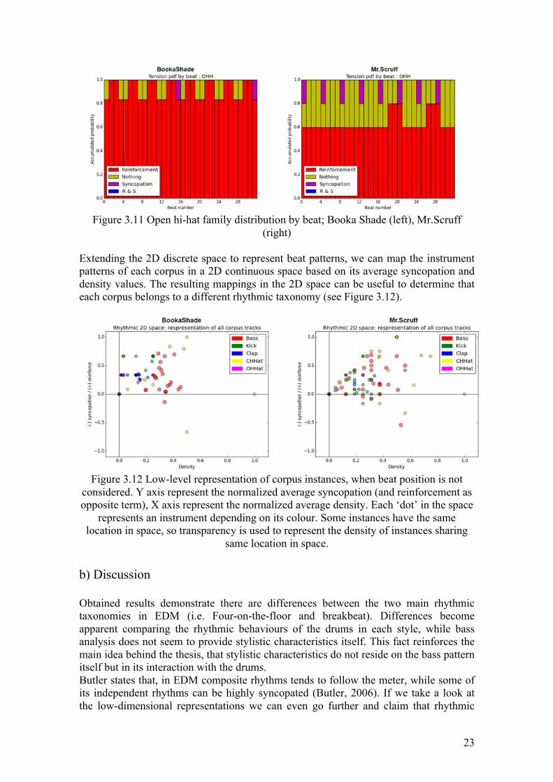
(right) Open Hi-hat: Comparing to previous instruments, the open hi-hat distributions don’t show prominent divergences (see Figure 3.11). The distribution temporal pattern is different comparing both distributions, but highly regular within the corpus itself.

23

Figure 3.11 Open hi-hat family distribution by beat; Booka Shade (left), Mr.Scruff

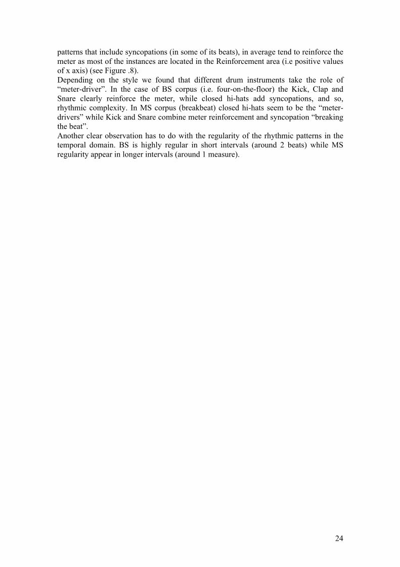
(right) Extending the 2D discrete space to represent beat patterns, we can map the instrument patterns of each corpus in a 2D continuous space based on its average syncopation and density values. The resulting mappings in the 2D space can be useful to determine that each corpus belongs to a different rhythmic taxonomy (see Figure 3.12).

Figure 3.12 Low-level representation of corpus instances, when beat position is not

considered. Y axis represent the normalized average syncopation (and reinforcement as opposite term), X axis represent the normalized average density. Each ‘dot’ in the space

represents an instrument depending on its colour. Some instances have the same location in space, so transparency is used to represent the density of instances sharing

same location in space. b) Discussion Obtained results demonstrate there are differences between the two main rhythmic taxonomies in EDM (i.e. Four-on-the-floor and breakbeat). Differences become apparent comparing the rhythmic behaviours of the drums in each style, while bass analysis does not seem to provide stylistic characteristics itself. This fact reinforces the main idea behind the thesis, that stylistic characteristics do not reside on the bass pattern itself but in its interaction with the drums. Butler states that, in EDM composite rhythms tends to follow the meter, while some of its independent rhythms can be highly syncopated (Butler, 2006). If we take a look at the low-dimensional representations we can even go further and claim that rhythmic

24

patterns that include syncopations (in some of its beats), in average tend to reinforce the meter as most of the instances are located in the Reinforcement area (i.e positive values of x axis) (see Figure .8). Depending on the style we found that different drum instruments take the role of “meter-driver”. In the case of BS corpus (i.e. four-on-the-floor) the Kick, Clap and Snare clearly reinforce the meter, while closed hi-hats add syncopations, and so, rhythmic complexity. In MS corpus (breakbeat) closed hi-hats seem to be the “meter-drivers” while Kick and Snare combine meter reinforcement and syncopation “breaking the beat”. Another clear observation has to do with the regularity of the rhythmic patterns in the temporal domain. BS is highly regular in short intervals (around 2 beats) while MS regularity appear in longer intervals (around 1 measure).

25

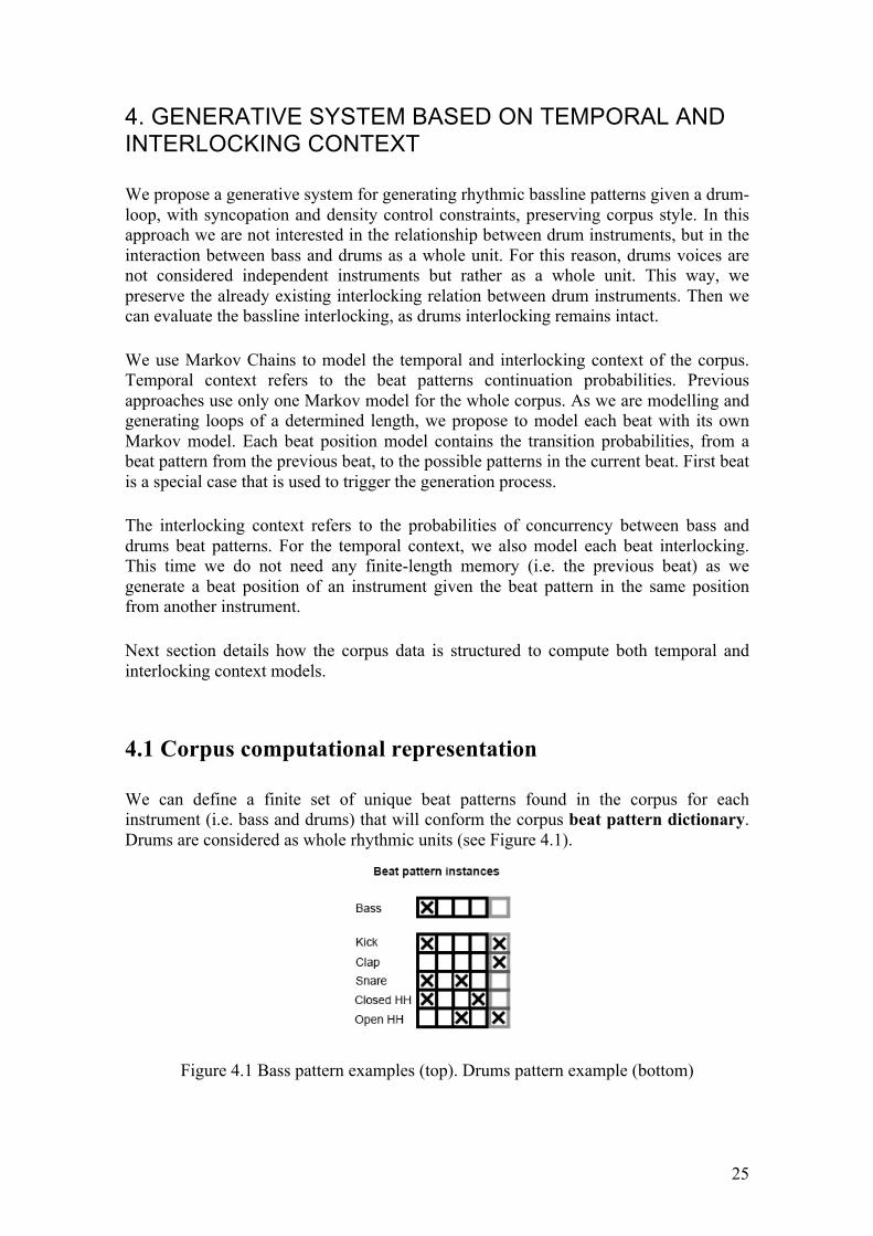
4. GENERATIVE SYSTEM BASED ON TEMPORAL AND INTERLOCKING CONTEXT We propose a generative system for generating rhythmic bassline patterns given a drum-loop, with syncopation and density control constraints, preserving corpus style. In this approach we are not interested in the relationship between drum instruments, but in the interaction between bass and drums as a whole unit. For this reason, drums voices are not considered independent instruments but rather as a whole unit. This way, we preserve the already existing interlocking relation between drum instruments. Then we can evaluate the bassline interlocking, as drums interlocking remains intact. We use Markov Chains to model the temporal and interlocking context of the corpus. Temporal context refers to the beat patterns continuation probabilities. Previous approaches use only one Markov model for the whole corpus. As we are modelling and generating loops of a determined length, we propose to model each beat with its own Markov model. Each beat position model contains the transition probabilities, from a beat pattern from the previous beat, to the possible patterns in the current beat. First beat is a special case that is used to trigger the generation process. The interlocking context refers to the probabilities of concurrency between bass and drums beat patterns. For the temporal context, we also model each beat interlocking. This time we do not need any finite-length memory (i.e. the previous beat) as we generate a beat position of an instrument given the beat pattern in the same position from another instrument. Next section details how the corpus data is structured to compute both temporal and interlocking context models. 4.1 Corpus computational representation We can define a finite set of unique beat patterns found in the corpus for each instrument (i.e. bass and drums) that will conform the corpus beat pattern dictionary. Drums are considered as whole rhythmic units (see Figure 4.1).

Figure 4.1 Bass pattern examples (top). Drums pattern example (bottom)

26

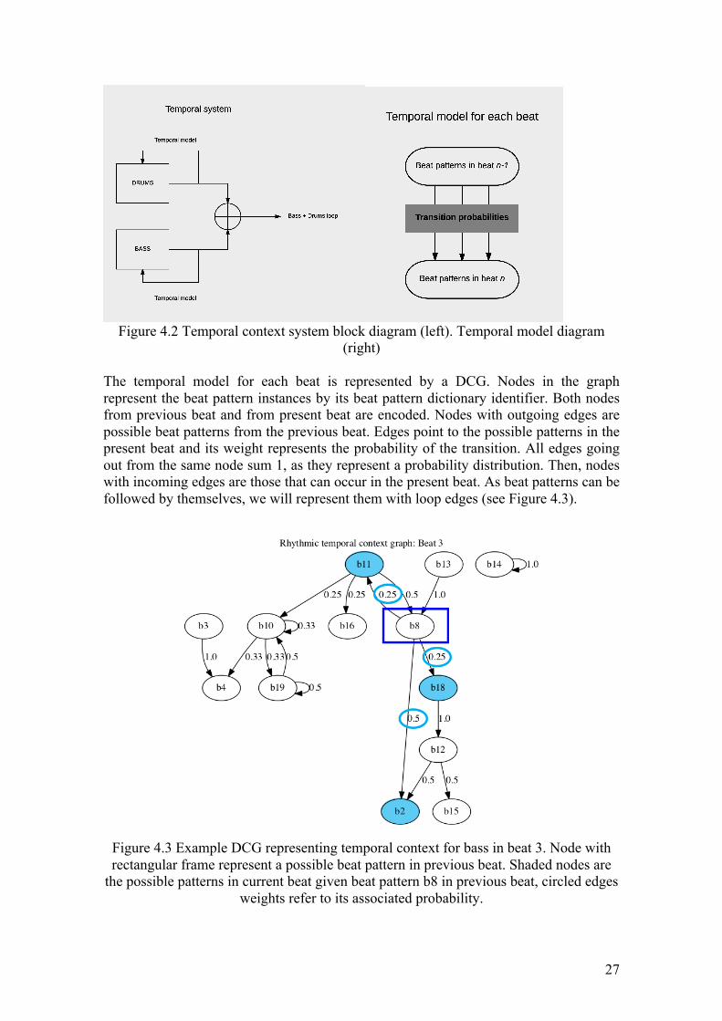
The maximum size of the dictionary is determined either by the time resolution and/or by the number of drum instruments. Each of the dictionary instances (unique patterns) and its associated information is encoded in a beat pattern class instance. The pattern class stores the following data structure: Beat pattern class: Beat location: Beat positions where the pattern was found (for each track) Track: Tracks where the pattern was found Pattern: Binary array representing onsets Syncopation value: Syncopation value for the given pattern Density: number of onsets in the pattern Once the dictionary for each instrument is built, we can re-encode the onset representation arrays, as arrays of indexes of pattern class instances. ‘Beat location’ and ‘track’ attributes are used to retrieve temporal and interlocking transition probabilities. Both temporal and interlocking models are represented using Directed Cyclic Graphs (DCG). Graphs provide a comprehensive representation of Markov chains; it is possible to visualize them and they are computationally simple. Each model will thus consist of L graphs, where L is the number of beats to model. Graph nodes are equivalent to MC states and represent pattern instances from the beat pattern dictionary previously computed. Edges represent pattern transition probabilities within the same instrument, or concurrency probabilities of patterns between instruments. We use the NetworkX12 python package to implement the models and to visualize them. 4.2 Temporal context model (TCM) The temporal model is computed independently for bass and drums. As mentioned, we model each beat position with its own model, in order to preserve the global temporal context. The local temporal context is then modelled by computing the transition probabilities between patterns from previous beat, and the patterns in the present (see Figure 4.2). A special case is the generation of the first beat, where we use the initial beat pattern probabilities from the corpus without any temporal constraints. As we are generating loops, it is necessary to generate the last beat, taking into account the first beat.

12 http:/newtworkx.github.io

27

Figure 4.2 Temporal context system block diagram (left). Temporal model diagram

(right) The temporal model for each beat is represented by a DCG. Nodes in the graph represent the beat pattern instances by its beat pattern dictionary identifier. Both nodes from previous beat and from present beat are encoded. Nodes with outgoing edges are possible beat patterns from the previous beat. Edges point to the possible patterns in the present beat and its weight represents the probability of the transition. All edges going out from the same node sum 1, as they represent a probability distribution. Then, nodes with incoming edges are those that can occur in the present beat. As beat patterns can be followed by themselves, we will represent them with loop edges (see Figure 4.3).

Figure 4.3 Example DCG representing temporal context for bass in beat 3. Node with rectangular frame represent a possible beat pattern in previous beat. Shaded nodes are

the possible patterns in current beat given beat pattern b8 in previous beat, circled edges weights refer to its associated probability.

28

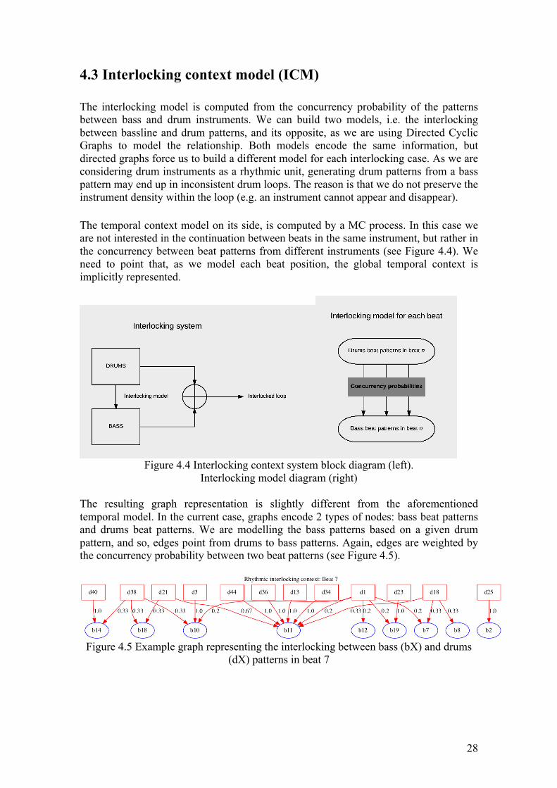
4.3 Interlocking context model (ICM) The interlocking model is computed from the concurrency probability of the patterns between bass and drum instruments. We can build two models, i.e. the interlocking between bassline and drum patterns, and its opposite, as we are using Directed Cyclic Graphs to model the relationship. Both models encode the same information, but directed graphs force us to build a different model for each interlocking case. As we are considering drum instruments as a rhythmic unit, generating drum patterns from a bass pattern may end up in inconsistent drum loops. The reason is that we do not preserve the instrument density within the loop (e.g. an instrument cannot appear and disappear). The temporal context model on its side, is computed by a MC process. In this case we are not interested in the continuation between beats in the same instrument, but rather in the concurrency between beat patterns from different instruments (see Figure 4.4). We need to point that, as we model each beat position, the global temporal context is implicitly represented.

Figure 4.4 Interlocking context system block diagram (left).

Interlocking model diagram (right) The resulting graph representation is slightly different from the aforementioned temporal model. In the current case, graphs encode 2 types of nodes: bass beat patterns and drums beat patterns. We are modelling the bass patterns based on a given drum pattern, and so, edges point from drums to bass patterns. Again, edges are weighted by the concurrency probability between two beat patterns (see Figure 4.5).

Figure 4.5 Example graph representing the interlocking between bass (bX) and drums

(dX) patterns in beat 7

29

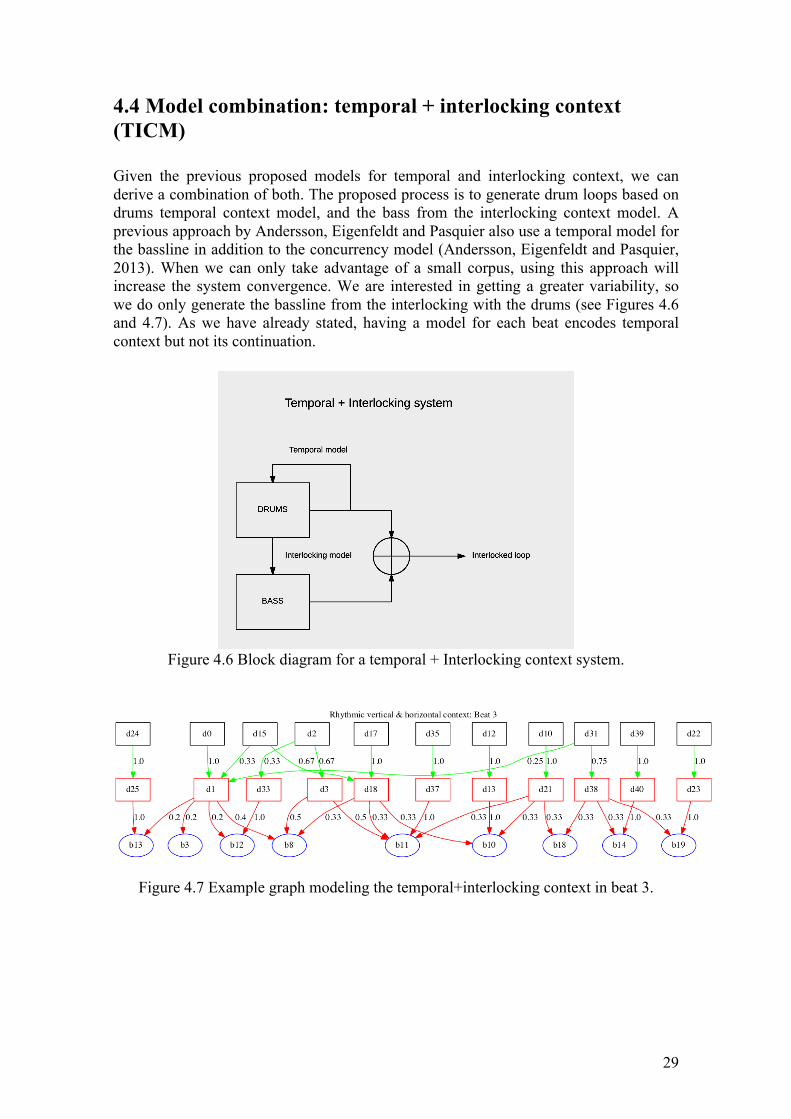
4.4 Model combination: temporal + interlocking context (TICM) Given the previous proposed models for temporal and interlocking context, we can derive a combination of both. The proposed process is to generate drum loops based on drums temporal context model, and the bass from the interlocking context model. A previous approach by Andersson, Eigenfeldt and Pasquier also use a temporal model for the bassline in addition to the concurrency model (Andersson, Eigenfeldt and Pasquier, 2013). When we can only take advantage of a small corpus, using this approach will increase the system convergence. We are interested in getting a greater variability, so we do only generate the bassline from the interlocking with the drums (see Figures 4.6 and 4.7). As we have already stated, having a model for each beat encodes temporal context but not its continuation.

Figure 4.6 Block diagram for a temporal + Interlocking context system.

Figure 4.7 Example graph modeling the temporal+interlocking context in beat 3.

30

4.5 Generation control model We propose a control model based on the knowledge extracted from the corpus. For each of the beat patterns in the collection, we know each syncopation and density values. In both models, the interlocking and temporal contexts encode the probability distribution between graph nodes. In other words, given a node with outgoing edges, we can “decide” between those nodes the edges point to. This “decision” is commonly driven by random sampling of the probability distribution. We propose to take advantage of the rhythmic information of “possible” nodes, so that we can drive the decision by high-level controls (e.g., to enhance syncopation, minimum density, etc.). Literature relates both syncopation and density to the induction of groove, but since this relation still requires a deeper understanding, we propose, for the moment, two independent controls for syncopation and density.

31

5. SYSTEM EVALUATION 5.1 Participants The experiment presented is a prototype of an ongoing experiment proposal. We carried out the experiment with 4 “test” users to evaluate the clarity of the instructions. The four “test” users have a musical background (i.e. play an instrument, interested in music), but only two of them are professional musicians. All the participants are in more or less grade familiar with EDM. 5.2 Design We want to test if there is a differential effect on the grooviness of a pattern, depending on the generation algorithm used. Then we test generated patters using ICM, TCM and, as a control condition to ensure that any of the algorithms truly provides an "improvement", random generation. This requires to fix a drum pattern and generate a bassline pattern using the three methods. The drum pattern is generated using the temporal context model (TCM) of a given corpus. The density and syncopation control parameters are not considered in this first experiment. The rating will be based on the grooviness perceived by the user using a Likert scale. Scale : 1-Not groovy at all! 2- Hardly groovy 3-Neutral 4-Danceable 5-Wanna dance! As the system is trained with dance music, generated results must preserve the feeling of groove. It is a subjective measure that will probably be affected by factors such as listening conditions, mental state, musical preferences, personality among others. However, literature state that groove perception relies on the cognitive system and not in cultural influence, so divergences between participants are expected to be minimized by means of cultural factors (e.g. age, genre preferences, country, and others). The system will be trained with both provided corpus: Booka Shade and Mr.Scruff. Both styles are considerably different when listening the original tracks. We hypothesize the output will preserve stylistic consistency, and so rhythm can be enough to discriminate music styles. While the two corpus styles use different tempo, instrument timbres and cues for stylistic differentiation, we fix both tempo and instrument timbres to synthesize both corpus’ outputs. 5.3 Materials For each style we generate 4 drum patterns using the TCM. For the same drum pattern, we generate three basslines using different generation methods. The first one is generated by the Interlocking context model (ICM), while the second is generated using bass TCM and so rhythmically independent of the drum loops. Third, a random rhythmic pattern to use as control. Taking into account we are evaluating two corpuses and we need 3 different bass patterns for a drum loop, we need to generate 24 instances.

32

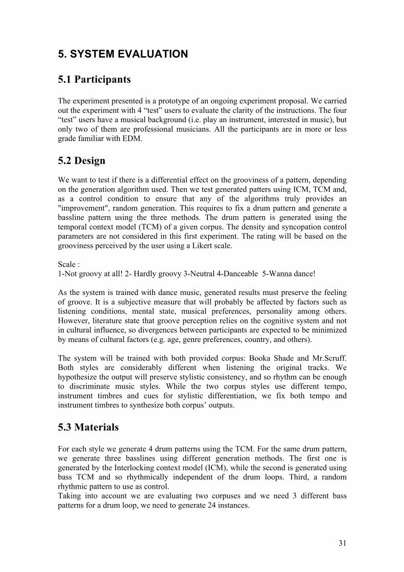
Drum patterns and its corresponding bass patterns will be synthesized and mixed using Ableton Live. The length of the loops will be 4 bars. 5.4 Procedure The experiment is presented as a google form and a set of audio files to evaluate. The following text is the introductory text presented to the user, exposing recommended conditions and the instructions to execute the experiment. Thanks for participating in this experiment, Before starting with the experiment instructions we recommend the following conditions: - Be in a quiet room - Use headphones - Use a media player application with "loop mode" - Enjoy! If you are not familiar with the term GROOVE: it is the property of rhythm that makes you want to dance - Download the audio files in the following link: https://drive.google.com/file/d/0B6U-zbLm43yPUXhMYTZXNjRfd1k/view?usp=sharing The experiment is divided in two sections: - First, fill in the initial questionnaire - Then, listen to each one of the provided audio files and rate its grooviness (see section after the initial questionnaire). Feel free to listen the audio files in loop and as many times as you want. It can also be helpful to stand up and dance if needed.

The initial questionnaire retrieves personal information of the subject to contextualize the results of the experiment. We ask for first for age and sex, to follow with a set of questions with a 5 point Likert scale. We are interested in:

• Familiarity of the subject with a set of EDM and non-EDM music genres (i.e EDM: House, Techno, Drum and bass, Hip-Hop)

• Experience composing rhythmic loops. • Preference for listening dance music. • Preference for dancing when listening to music • Preference for attending to dance music clubs/concerts/festivals?

Loops are presented as audio files in a downloadable folder. For this experiment we will use three different playlist permutations, randomizing the two variables in the experiment (i.e. generation method and style). Each loop need to be rated using the

33

proposed Likert scale associated to grooviness (see Figure 4.8). Listeners can listen (and ideally loop) each of the audio files multiple times, and so, change its rating.

Figure 4.8 Likert scale for rating grooviness of each audio file

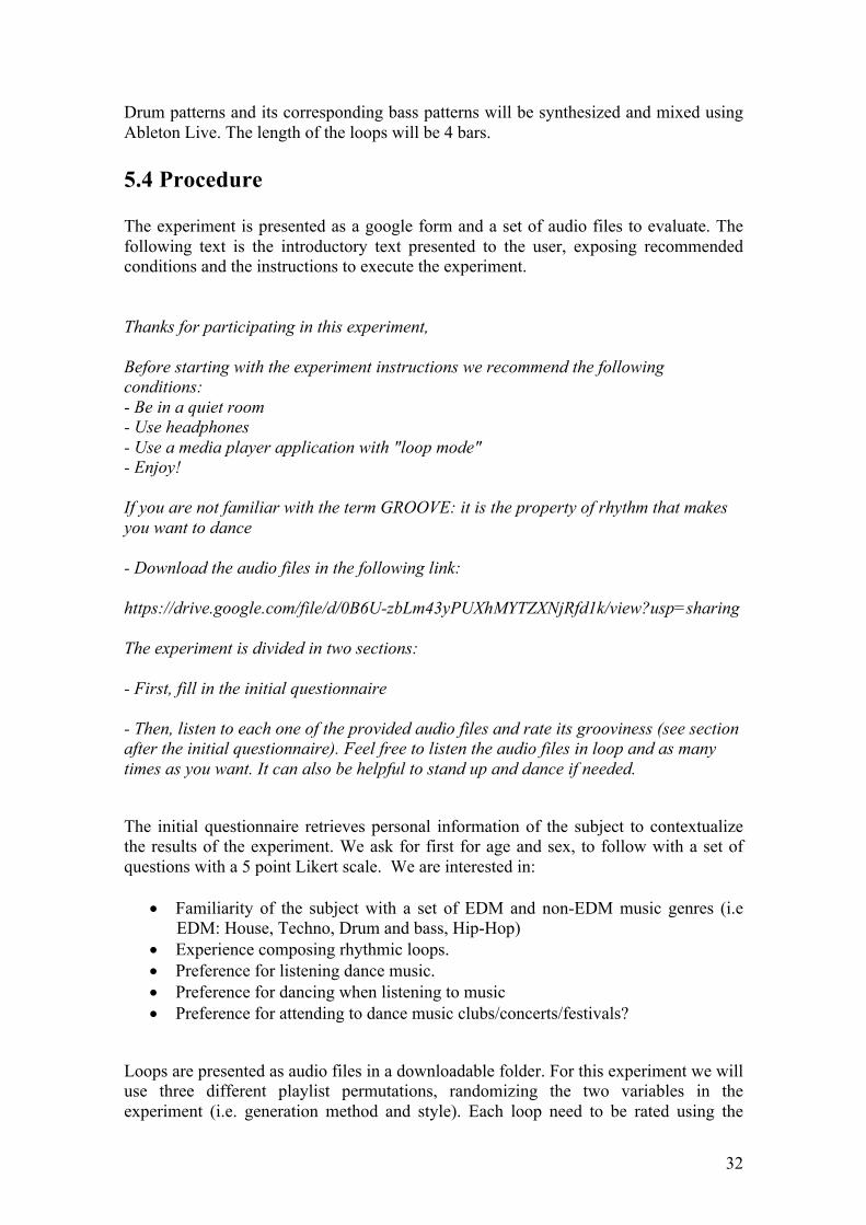
5.5 Results As a first result of the analysis we can compute the statistic of the ratings for each of the generation methods (see Figure 4.9). For now, as we are concerned of evaluating the clarity of the experiment results are not as important as the feedback provided by users. Results are not statistically relevant (only 5 users) but set the baseline for next evaluations. The interlocking method that we are interested to evaluate has a prominent grading of “Danceable”, however the random method gives a similar grading distribution.

Figure 4.9 Statistics of grooviness rating for each generation method

34

5.6 Discussion Most users found it was a difficult task to rate the grooviness of the loops. While the concept of grooviness was clear to them, most point out that all the loops having the same timbre was confusing (and boring). The “professional musicians” also pointed that it was noticeable a lack of swing in the drums, feature they consider crucial for groove induction. Obtained results encourage further experimentation improving the current experimentation proposal.

35

6. CONCLUSIONS As seen in chapter 3, the proposed analysis methodology makes possible to represent rhythmic patterns of different instruments in the same geometrical space. In addition to provide a graphical representation of the problem, the geometrical mapping of rhythmic patterns allows to study each of the instruments to determine its “function” within each style. Resulting analysis for each of the corpus revealed clearly that they belong to different rhythmic taxonomies (i.e. four-on-the-floor and breakbeat). We found that most relevant differences occur in the Kick and Clap/Snare rhythmic patterns; while in the Book Shade corpus (four-on-the-floor) they are regular and clearly reinforce the meter, in the Mr.Scruff corpus (breakbeat) they are significantly less regular and with higher rhythmic complexity. These observations coincide with the definition of the rhythmic taxonomy that represent each style. In chapter 4 we present three methodologies for bass and drum pattern generation within a given style determined by the seed corpus. Even though the evaluation of the system methodologies is still in development, we consider a satisfactory achievement the accomplishment of a tractable generative system for rhythmic interlocking with parametrical controls. Previous approaches using Markov Chains methods didn’t exploit the idea of modelling each of the beats independently to preserve the global temporal context of the style. This contribution helps to attenuate the “short-memory” of order-1 Markov processes that in practice drive into the generation of incoherent rhythmic phrases. Moreover, getting rid of previous approaches that encode MC as matrices, we took advantage of graphs to propose an optimal computational model that can be also visualized. Throughout this thesis we established a self-contained framework for analysis, visualization and generation of rhythmic interlocking that can be the starting point for future research on the topic. As mentioned before, this thesis only grasps the surface of theorizing the rhythmic interactions between instruments in different music styles. Presented achievements encourage the study of rhythmic interlocking using more styles, each represented with bigger datasets, to demonstrate that the proof-of-concept exposed in this thesis can be generalized to other music styles. The obtention of new datasets will require an automatic transcription methodology able to build datasets without human intervention. The proposed generative system has been implemented as an offline system for fast prototyping, however it can be extended to a real-time implementation where the controls are not global anymore, but controlled in real-time. As shown in section 4.6 the evaluation of a system that generates “musical” output using user-centered experiments is not an easy task. New experiment methodologies should be designed to experimentally validate the results of the proposed generative methodologies. In addition, the proposed 2D rhythmic space can be useful for applying topological analysis techniques, opposed to analyse rhythms as binary streams of onsets, giving a more comprehensive approach.

37

BIBLIOGRAPHY

Ames, C. (2011). Automated Composition in Retrospect: 1956-1986, 20(2), 169–185.

Ames, C. (1989). The Markov Process as a Compositional Model : A Survey and Tutorial. Leonardo, 22(2), 175–187.

Ames, C., & Domino, M. (1992). Understanding music with AI, chap. Cybernetic composer: an overview, pp. 186–205. The MIT Press, Cambridge.

Anderson, C., Eigenfeldt, A., & Pasquier, P. (2013). The Generative Electronic Dance Music Algorithmic System (GEDMAS). Proceedings of the Second International Workshop on Musical Metacreation (MUME-2013), in Conjunction with the Ninth Annual AAAI Conference on Artificial Intelligence and Interactive Digital Entertainment (AIIDE-13), 5–8.

Butler, M. J. (2006). Unlocking the Groove.

Cao, E., Lotstein, M., & Johnson-Laird, P. N. (2014). similarity and families of musical rhythms. Music Perception: An Interdisciplinary Journal, 31(5), 444–469.

de Cheveigné, A., & Kawahara, H. (2002). YIN, a fundamental frequency estimator for speech and music. The Journal of the Acoustical Society of America, 111(4), 1917–1930. http://doi.org/10.1121/1.1458024

Cont, A., Dubnov, S., & Assayag, G. (2007). Anticipatory model of musical style imitation using collaborative and competitive reinforcement learning. Lecture Notes in Computer Science, 4520, 285–306. http://doi.org/10.1007/978-3-540-74262-3_16

Dubnov, S., Assayag, G., Lartillot, O., & Bejerano, G. (2003). Using machine-learning methods for musical style modeling. Computer, 36(10), 73–80. http://doi.org/10.1109/MC.2003.1236474

Eigenfeldt, A., & Pasquier, P. (2013). Considering Vertical and Horizontal Context in Corpus-based Generative Electronic Dance Music. Creativity, 72–78.

Essens, P. (1995). Structuring temporal sequences: Comparison of models and factors of complexity. Perception and Psychophysics, 57, 519-532.

Fernández, J. D., & Vico, F. (2013). Ai methods in algorithmic composition: A comprehensive survey. Journal of Artificial Intelligence Research. http://doi.org/10.1613/jair.3908

Gómez-Marín, D., Jordà, S., and Herrera, P. (2015a). Pad and Sad: Two awareness-Weighted rhythmic similarity distances. In 16th International Society for Music Information Retrieval Conf. ISMIR.

38

Gómez-Marín, D., Jordà, S., and Herrera, P. (2015b). Strictly Rhythm: Exploring the effects of identical regions and meter induction in rhythmic similarity perception. In 11th International Symposium on Computer Music Multidisciplinary Research (CMMR), Plymouth.

Goto, M. (2004). A real-time music-scene-description system: predominant-F0 estimation for detecting melody and bass lines in real-world audio signals. Speech Communication, 43(4), 311–329. http://doi.org/10.1016/j.specom.2004.07.001

Holm, T., & Isaksson, T. (2010). Syncopes, duration and timing properties used to affect groove in monophonic melodies. Umu.Diva-Portal.Org. Retrieved from http://umu.diva-portal.org/smash/get/diva2:346179/FULLTEXT01

Johnson-Laird, P. N. (1991). Rhythm and meter: A theory at the computational level. Psychomusicology: A Journal of Research in Music Cognition, 10(2), 88–106. http://doi.org/10.1037/h0094139

Lerdahl, F., & Jackendoff, R. S. (1996). A Generative Theory of Tonal Music MIT Press Series On Cognitive Theory and Mental Representation. MIT Press.

Longuet-Higgins, H. C., & Lee, C. S. (1984). The Rhythmic Interpretation of Monophonic Music. Music Perception: An Interdisciplinary Journal, 1(4), 424–441. http://doi.org/10.2307/40285271

Lyon, D. (1995). Using stochastic Petri nets for real-time Nth-order stochastic composition. Computer Music Journal, 19(4), 13–22.

Moorer, J. A. (1972). Music and computer composition. Communications of the ACM, 15(2), 104–113.

North, T. (1991). A technical explanation of theme and variations: A computer music work utilizing network compositional algorithms. Ex Tempore, 5(2).

Pachet, F. (2002). The Continuator: Musical Interaction With Style. Journal of New Music Research, 31(1), 333–341. http://doi.org/10.1076/jnmr.32.3.333.16861

Pachet, F., Roy, P., & Barbieri, G. (2011). Finite-length Markov processes with constraints. IJCAI International Joint Conference on Artificial Intelligence, 635–642. http://doi.org/10.5591/978-1-57735-516-8/IJCAI11-113

Povel, D-J. (1984). A theoretical framework for rhythm perception. Psychological Research, 45, 315-337.

Salamon, J., & Gomez, E. (2009). A Chroma-based Salience Function for Melody and Bass Line Estimation from Music Audio Signals. Sound and Music Computing, (July), 331–336. Retrieved from http://www.mtg.upf.edu/node/1329

Salamon, J. (2013). Melody Extraction from Polyphonic Music Signals, 20(6), 1759–1770.

39

Volk, A. (2008). The study of syncopation using inner metric analysis: Linking theoretical and experimental analysis of metre in music. Journal of New Music Research, 37, 259-273. Werner, M., & Todd, P. M. (1997). Too many love songs: Sexual selection and the evolution of communication. In Proceedings of the European Conference on Artificial Life.

41

APPENDIX

42

SOFTWARE We deliver the current Python package that is still under development. It provides a simple GUI-based application example and some examples of usage. The main package contains two sub-packages that implement the corpus analysis and the generation methods.

This first prototype consists of two main modules:

• The analysis module extracts rhythmic features and computes the temporal and interlocking context models of an input corpus. It can export the computed graph model as an image ( *.png ) or as a Yaml13 file. The extracted data is also stored using the Pickle14 library to serialize python objects, so that the data can be shared with the generation module.

• The generation module provides a first approach of a graph-constrained model. It takes its input from the graph representation computed by the analysis module.

We also provide the transcribed datasets and the RIV Max application. Source code: https://drive.google.com/open?id=0B0inSllIuGQUMFJnWjdJNWxteGs

• Rhythm_Visualization.zip : RIV Max application • BookaShade_Interlocking_dataset.zip: Transcribed dataset • MrScruff_Interlocking_dataset.zip: Transcribed dataset • GS_Bass_Drums_Interlocking-v1.zip: Pyhton package for rhythmic analysis

and generation

13 http://yaml.org 14 https://docs.python.org/2/library/pickle.html

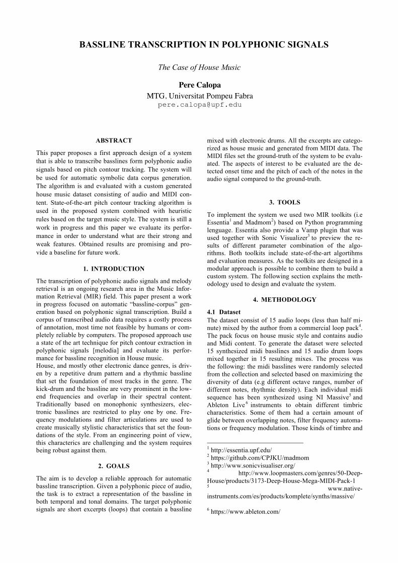
BASSLINE TRANSCRIPTION IN POLYPHONIC SIGNALS

The Case of House Music

Pere Calopa MTG, Universitat Pompeu Fabra

[email protected]

ABSTRACT

This paper proposes a first approach design of a system that is able to transcribe basslines form polyphonic audio signals based on pitch contour tracking. The system will be used for automatic symbolic data corpus generation. The algorithm is and evaluated with a custom generated house music dataset consisting of audio and MIDI con-tent. State-of-the-art pitch contour tracking algorithm is used in the proposed system combined with heuristic rules based on the target music style. The system is still a work in progress and this paper we evaluate its perfor-mance in order to understand what are their strong and weak features. Obtained results are promising and pro-vide a baseline for future work.

1. INTRODUCTION

The transcription of polyphonic audio signals and melody retrieval is an ongoing research area in the Music Infor-mation Retrieval (MIR) field. This paper present a work in progress focused on automatic “bassline-corpus” gen-eration based on polyphonic signal transcription. Build a corpus of transcribed audio data requires a costly process of annotation, most time not feasible by humans or com-pletely reliable by computers. The proposed approach use a state of the art technique for pitch contour extraction in polyphonic signals [melodia] and evaluate its perfor-mance for bassline recognition in House music. House, and mostly other electronic dance genres, is driv-en by a repetitive drum pattern and a rhythmic bassline that set the foundation of most tracks in the genre. The kick-drum and the bassline are very prominent in the low-end frequencies and overlap in their spectral content. Traditionally based on monophonic synthesizers, elec-tronic basslines are restricted to play one by one. Fre-quency modulations and filter articulations are used to create musically stylistic characteristics that set the foun-dations of the style. From an engineering point of view, this characterics are challenging and the system requires being robust against them.

2. GOALS

The aim is to develop a reliable approach for automatic bassline transcription. Given a polyphonic piece of audio, the task is to extract a representation of the bassline in both temporal and tonal domains. The target polyphonic signals are short excerpts (loops) that contain a bassline

mixed with electronic drums. All the excerpts are catego-rized as house music and generated from MIDI data. The MIDI files set the ground-truth of the system to be evalu-ated. The aspects of interest to be evaluated are the de-tected onset time and the pitch of each of the notes in the audio signal compared to the ground-truth.

3. TOOLS

To implement the system we used two MIR toolkits (i.e Essentia1 and Madmom2) based on Python programming lenguage. Essentia also provide a Vamp plugin that was used together with Sonic Visualizer3 to preview the re-sults of different parameter combination of the algo-rithms. Both toolkits include state-of-the-art algortihms and evaluation measures. As the toolkits are designed in a modular approach is possible to combine them to build a custom system. The following section explains the meth-odology used to design and evaluate the system.

4. METHODOLOGY

4.1 Dataset The dataset consist of 15 audio loops (less than half mi-nute) mixed by the author from a commercial loop pack4. The pack focus on house music style and contains audio and Midi content. To generate the dataset were selected 15 synthesized midi basslines and 15 audio drum loops mixed together in 15 resulting mixes. The process was the following: the midi basslines were randomly selected from the collection and selected based on maximizing the diversity of data (e.g different octave ranges, number of different notes, rhythmic density). Each individual midi sequence has been synthesized using NI Massive5 and Ableton Live 6 instruments to obtain different timbric characteristics. Some of them had a certain amount of glide between overlapping notes, filter frequency automa-tions or frequency modulation. Those kinds of timbre and

1 http://essentia.upf.edu/ 2 https://github.com/CPJKU/madmom 3 http://www.sonicvisualiser.org/ 4 http://www.loopmasters.com/genres/50-Deep-House/products/3173-Deep-House-Mega-MIDI-Pack-1 5 www.native-instruments.com/es/products/komplete/synths/massive/ 6 https://www.ableton.com/

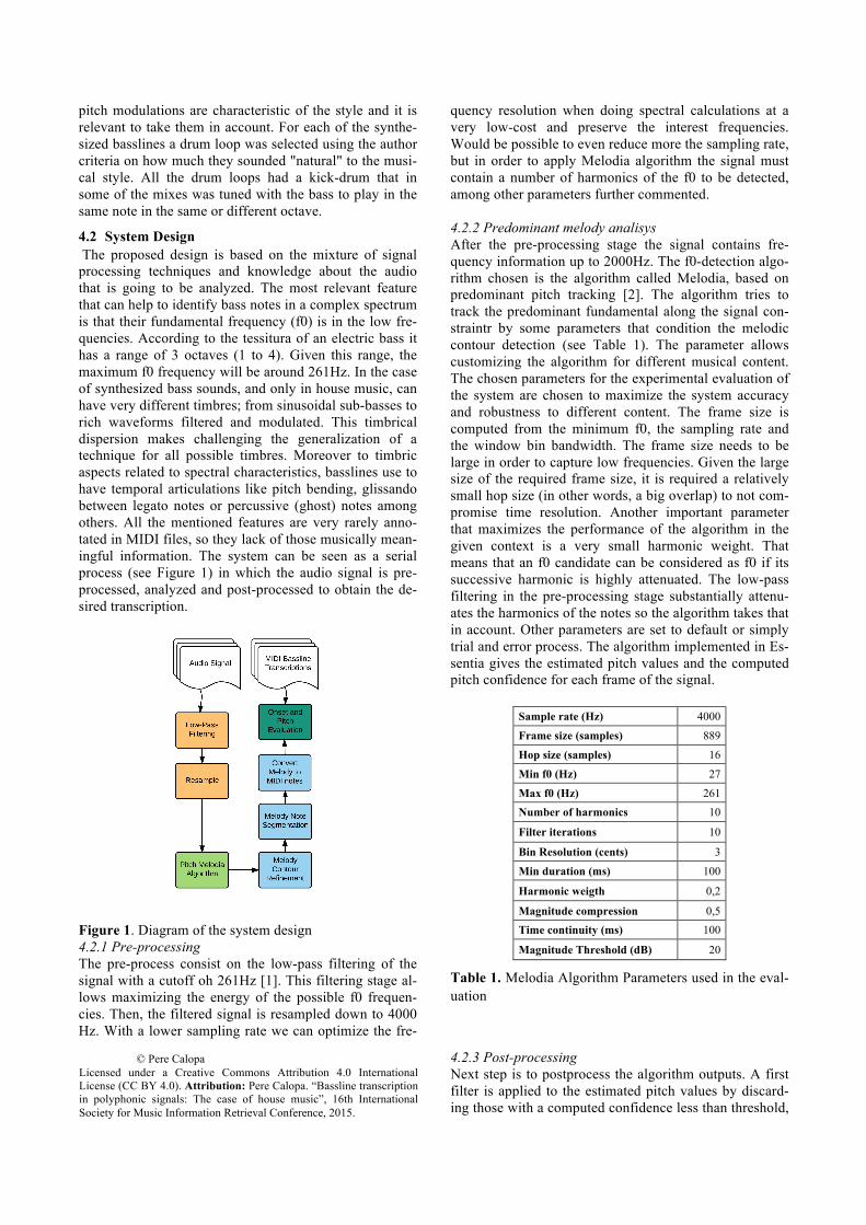
pitch modulations are characteristic of the style and it is relevant to take them in account. For each of the synthe-sized basslines a drum loop was selected using the author criteria on how much they sounded "natural" to the musi-cal style. All the drum loops had a kick-drum that in some of the mixes was tuned with the bass to play in the same note in the same or different octave.

4.2 System Design The proposed design is based on the mixture of signal processing techniques and knowledge about the audio that is going to be analyzed. The most relevant feature that can help to identify bass notes in a complex spectrum is that their fundamental frequency (f0) is in the low fre-quencies. According to the tessitura of an electric bass it has a range of 3 octaves (1 to 4). Given this range, the maximum f0 frequency will be around 261Hz. In the case of synthesized bass sounds, and only in house music, can have very different timbres; from sinusoidal sub-basses to rich waveforms filtered and modulated. This timbrical dispersion makes challenging the generalization of a technique for all possible timbres. Moreover to timbric aspects related to spectral characteristics, basslines use to have temporal articulations like pitch bending, glissando between legato notes or percussive (ghost) notes among others. All the mentioned features are very rarely anno-tated in MIDI files, so they lack of those musically mean-ingful information. The system can be seen as a serial process (see Figure 1) in which the audio signal is pre-processed, analyzed and post-processed to obtain the de-sired transcription.

Figure 1. Diagram of the system design 4.2.1 Pre-processing The pre-process consist on the low-pass filtering of the signal with a cutoff oh 261Hz [1]. This filtering stage al-lows maximizing the energy of the possible f0 frequen-cies. Then, the filtered signal is resampled down to 4000 Hz. With a lower sampling rate we can optimize the fre-

quency resolution when doing spectral calculations at a very low-cost and preserve the interest frequencies. Would be possible to even reduce more the sampling rate, but in order to apply Melodia algorithm the signal must contain a number of harmonics of the f0 to be detected, among other parameters further commented. 4.2.2 Predominant melody analisys After the pre-processing stage the signal contains fre-quency information up to 2000Hz. The f0-detection algo-rithm chosen is the algorithm called Melodia, based on predominant pitch tracking [2]. The algorithm tries to track the predominant fundamental along the signal con-straintr by some parameters that condition the melodic contour detection (see Table 1). The parameter allows customizing the algorithm for different musical content. The chosen parameters for the experimental evaluation of the system are chosen to maximize the system accuracy and robustness to different content. The frame size is computed from the minimum f0, the sampling rate and the window bin bandwidth. The frame size needs to be large in order to capture low frequencies. Given the large size of the required frame size, it is required a relatively small hop size (in other words, a big overlap) to not com-promise time resolution. Another important parameter that maximizes the performance of the algorithm in the given context is a very small harmonic weight. That means that an f0 candidate can be considered as f0 if its successive harmonic is highly attenuated. The low-pass filtering in the pre-processing stage substantially attenu-ates the harmonics of the notes so the algorithm takes that in account. Other parameters are set to default or simply trial and error process. The algorithm implemented in Es-sentia gives the estimated pitch values and the computed pitch confidence for each frame of the signal.

Sample rate (Hz) 4000

Frame size (samples) 889

Hop size (samples) 16

Min f0 (Hz) 27

Max f0 (Hz) 261 Number of harmonics 10

Filter iterations 10

Bin Resolution (cents) 3

Min duration (ms) 100

Harmonic weigth 0,2

Magnitude compression 0,5 Time continuity (ms) 100

Magnitude Threshold (dB) 20

Table 1. Melodia Algorithm Parameters used in the eval-uation

4.2.3 Post-processing Next step is to postprocess the algorithm outputs. A first filter is applied to the estimated pitch values by discard-ing those with a computed confidence less than threshold,

© Pere Calopa Licensed under a Creative Commons Attribution 4.0 International License (CC BY 4.0). Attribution: Pere Calopa. “Bassline transcription in polyphonic signals: The case of house music”, 16th International Society for Music Information Retrieval Conference, 2015.

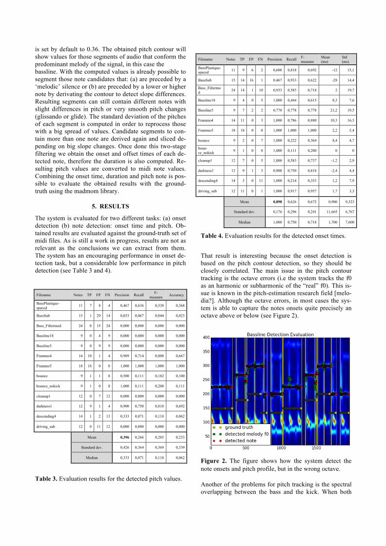
is set by default to 0.36. The obtained pitch contour will show values for those segments of audio that conform the predominant melody of the signal, in this case the bassline. With the computed values is already possible to segment those note candidates that: (a) are preceded by a ‘melodic’ silence or (b) are preceded by a lower or higher note by derivating the contour to detect slope differences. Resulting segments can still contain different notes with slight differences in pitch or very smooth pitch changes (glissando or glide). The standard deviation of the pitches of each segment is computed in order to reprocess those with a big spread of values. Candidate segments to con-tain more than one note are derived again and sliced de-pending on big slope changes. Once done this two-stage filtering we obtain the onset and offset times of each de-tected note, therefore the duration is also computed. Re-sulting pitch values are converted to midi note values. Combining the onset time, duration and pitch note is pos-sible to evaluate the obtained results with the ground-truth using the madmom library.

5. RESULTS

The system is evaluated for two different tasks: (a) onset detection (b) note detection: onset time and pitch. Ob-tained results are evaluated against the ground-truth set of midi files. As is still a work in progress, results are not as relevant as the conclusions we can extract from them. The system has an encouraging performance in onset de-tection task, but a considerable low performance in pitch detection (see Table 3 and 4). Filename Notes TP FP FN Precision Recall F-

measure Accuracy

BassPlastique-spaced 11 7 8 4 0,467 0,636 0,538 0,368

BassSub 15 1 29 14 0,033 0,067 0,044 0,023

Bass_Filtermod 24 0 15 24 0,000 0,000 0,000 0,000

Bassline18 9 0 4 9 0,000 0,000 0,000 0,000

Bassline5 9 0 9 9 0,000 0,000 0,000 0,000

Frammo4 14 10 1 4 0,909 0,714 0,800 0,667

Frammo5 18 18 0 0 1,000 1,000 1,000 1,000

bounce 9 1 1 8 0,500 0,111 0,182 0,100

bounce_nokick 9 1 0 8 1,000 0,111 0,200 0,111

cleanup1 12 0 7 12 0,000 0,000 0,000 0,000

darkness1 12 9 1 4 0,900 0,750 0,818 0,692

descending4 14 1 2 13 0,333 0,071 0,118 0,062

driving_sub 12 0 11 12 0,000 0,000 0,000 0,000

Mean 0,396 0,266 0,285 0,233

Standard dev. 0,426 0,364 0,369 0,339

Median 0,333 0,071 0,118 0,062

Table 3. Evaluation results for the detected pitch values.

Filename Notes TP FP FN Precision Recall F-

measure Mean (ms)

Std (ms)

BassPlastique-spaced 11 9 6 2 0,600 0,818 0,692 -12 15,1

BassSub 15 14 16 1 0,467 0,933 0,622 -28 14,4

Bass_Filtermod 24 14 1 10 0,933 0,583 0,718 2 19,7

Bassline18 9 4 0 5 1,000 0,444 0,615 8,3 7,6

Bassline5 9 7 2 2 0,778 0,778 0,778 21,2 19,5

Frammo4 14 11 0 3 1,000 0,786 0,880 10,3 16,3

Frammo5 18 18 0 0 1,000 1,000 1,000 2,2 5,4

bounce 9 2 0 7 1,000 0,222 0,364 8,4 4,7

boun-ce_nokick 9 1 0 8 1,000 0,111 0,200 0 0

cleanup1 12 7 0 5 1,000 0,583 0,737 -1,2 2,9

darkness1 12 9 1 3 0,900 0,750 0,818 -2,4 4,4

descending4 14 3 0 11 1,000 0,214 0,353 1,2 7,9

driving_sub 12 11 0 1 1,000 0,917 0,957 1,7 3,3

Mean 0,898 0,626 0,672 0,900 9,323

Standard dev. 0,176 0,296 0,241 11,665 6,767

Median 1,000 0,750 0,718 1,700 7,600

Table 4. Evaluation results for the detected onset times.

That result is interesting because the onset detection is based on the pitch contour detection, so they should be closely correlated. The main issue in the pitch contour tracking is the octave errors (i.e the system tracks the f0 as an harmonic or subharmonic of the “real” f0). This is-sue is known in the pitch-estimation research field [melo-dia?]. Although the octave errors, in most cases the sys-tem is able to capture the notes onsets quite precisely an octave above or below (see Figure 2).

Figure 2. The figure shows how the system detect the note onsets and pitch profile, but in the wrong octave. Another of the problems for pitch tracking is the spectral overlapping between the bass and the kick. When both

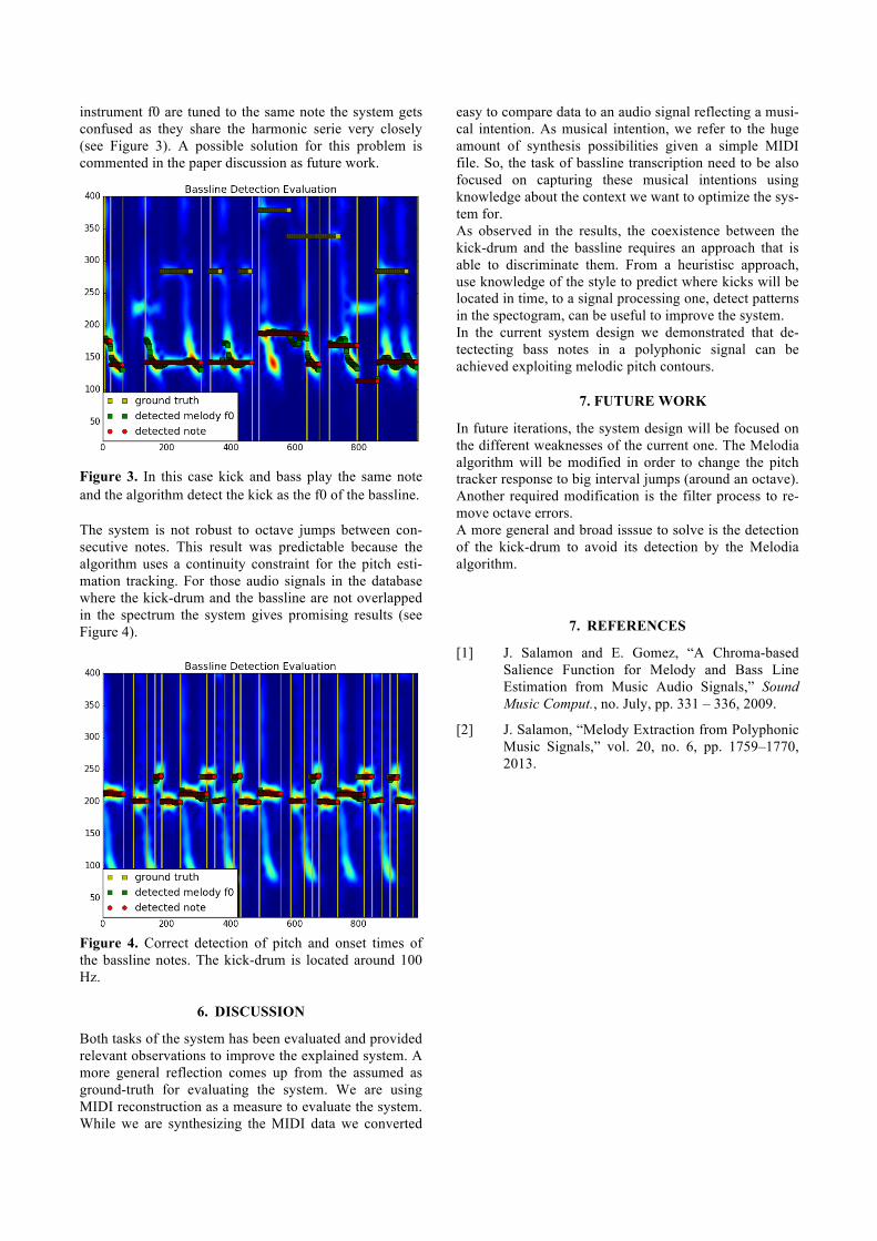
instrument f0 are tuned to the same note the system gets confused as they share the harmonic serie very closely (see Figure 3). A possible solution for this problem is commented in the paper discussion as future work.

Figure 3. In this case kick and bass play the same note and the algorithm detect the kick as the f0 of the bassline. The system is not robust to octave jumps between con-secutive notes. This result was predictable because the algorithm uses a continuity constraint for the pitch esti-mation tracking. For those audio signals in the database where the kick-drum and the bassline are not overlapped in the spectrum the system gives promising results (see Figure 4).

Figure 4. Correct detection of pitch and onset times of the bassline notes. The kick-drum is located around 100 Hz.

6. DISCUSSION

Both tasks of the system has been evaluated and provided relevant observations to improve the explained system. A more general reflection comes up from the assumed as ground-truth for evaluating the system. We are using MIDI reconstruction as a measure to evaluate the system. While we are synthesizing the MIDI data we converted

easy to compare data to an audio signal reflecting a musi-cal intention. As musical intention, we refer to the huge amount of synthesis possibilities given a simple MIDI file. So, the task of bassline transcription need to be also focused on capturing these musical intentions using knowledge about the context we want to optimize the sys-tem for. As observed in the results, the coexistence between the kick-drum and the bassline requires an approach that is able to discriminate them. From a heuristisc approach, use knowledge of the style to predict where kicks will be located in time, to a signal processing one, detect patterns in the spectogram, can be useful to improve the system. In the current system design we demonstrated that de-tectecting bass notes in a polyphonic signal can be achieved exploiting melodic pitch contours.

7. FUTURE WORK

In future iterations, the system design will be focused on the different weaknesses of the current one. The Melodia algorithm will be modified in order to change the pitch tracker response to big interval jumps (around an octave). Another required modification is the filter process to re-move octave errors. A more general and broad isssue to solve is the detection of the kick-drum to avoid its detection by the Melodia algorithm.

7. REFERENCES

[1] J. Salamon and E. Gomez, “A Chroma-based Salience Function for Melody and Bass Line Estimation from Music Audio Signals,” Sound Music Comput., no. July, pp. 331 – 336, 2009.

[2] J. Salamon, “Melody Extraction from Polyphonic Music Signals,” vol. 20, no. 6, pp. 1759–1770, 2013.

Drums and Bass Interlocking

Documents

Transcript of Drums and Bass Interlocking