1

Drogue Dynamic Model under Bow Wave inProbe-and-drogue Refueling

Zi-Bo Wei, Xunhua Dai, Quan Quan, and Kai-Yuan Cai

Abstract—Probe-and-drogue refueling (PDR) is widelyadopted owing to its simple requirement of equipment andflexibility, but it has an apparent drawback that the drogueposition is susceptible to disturbances. There are threetypes of disturbances: atmospheric turbulence, trailingvortex of the tanker, and bow wave effect caused by thereceiver. The former two disturbances are independent ofthe receiver, whereas the bow wave effect, which dependson the state of the receiver, influences the docking greatlywithin a close distance. As far as authors know, littleattention was paid to the bow wave effect on dockingcontrol in existing literature. The existing literature relatedto the bow wave focuses on either qualitative static resultsobtained from experiments, or lookup tables based oncomputational fluid dynamics (CFD) analysis. These areinapplicable to the PDR docking controller design directly.For such a reason, this paper proposes a lower-orderdynamic model to describe drogue dynamics under thebow wave effect. The model consists of two components:one is a 2nd-order transfer function matrix to describe thedrogue dynamics, and the other is a nonlinear functionvector to describe the bow wave effect model. A closed-loop simulation including the two components shows thatthe generated drogue dynamics are similar to those of areal experiment reported in an existing literature.

Index Terms—Aerial refueling, probe-and-drogue, bowwave, towed cable system, dynamic model.

NOMENCLATURE

oi − xiyizi = inertial frame with axes(xi, yi, zi)

ot − xtytzt = frame fixed to the conjunctivepoint between the tanker andthe hosewith axes (xt, yt, zt)

or − xryrzr = frame fixed to the mass centerof the receiver with axes(xr, yr, zr)

This work was supported by the National Natural Science Foun-dation of China under Grant 61473012.

The authors are with School of Automation Science and ElectricalEngineering, Beihang University, Beijing 100191, China (e-mail:whisper@buaa.edu.cn; dai@buaa.edu.cn; qq buaa@buaa.edu.cn; ky-cai@buaa.edu.cn)

of − xfyfzf = frame fixed to the cockpitof the receiver with axes(xf , yf , zf ) and used ina CFD software

θr/t = Euler angle vector describingthe rotation from ot − xtytztto or − xryrzr, deg

θr/i = Euler angle vector describingthe rotation from oi − xiyizito or − xryrzr, deg

vt = velocity vector of the tanker, m/sv = refueling velocity, m/sh = refueling altitude, mLj = the jth linklj = length of Lj , mldr = length of the drogue, mpLj

= position vector of the end of Lj , mpr = position vector of the mass center

of the receiver, mpd = position vector of the center of

the drogue canopy, mpp = position vector of the probe’s

fore-end, mpf = position vector of the origin of

the CFD frame, mpn = position vector of the nose’s

fore-end of the receiver, mf b = force vector of the bow wave

effect acting on the drogue, Nfa = force vector of atmospheric

turbulence, Nf v = force vector of the trailing

vortex of the tanker, NR2 = coefficient of determinationαj, βj = orientation angles of Lj , degCFD = Computational Fluid DynamicsGBN = Generalized Binary NoiseNASA = National Aeronautics and

Space AdministrationNATO = North Atlantic Treaty OrganizationPDR = Probe-and-drogue Refueling

2

I. INTRODUCTION

Air to air refuelling is an effective method ofincreasing the endurance and range of aircraft by re-fuelling them in flight [1]. In addition, by refueling,aircraft are able to carry their maximum payloadwithout reducing their range [2]. There are twomajor aerial refueling systems in operation today:the Boeing’s “Flying Boom” system and the Cob-ham’s “Probe-and-drogue” system [3]. The probe-and-drogue system is widely adopted owing to itssimple requirement of equipment and flexibility.In the probe-and-drogue system, a tanker aircraftreleases a flexible hose which terminates in a conicalshaped drogue and trails behind the tanker aircraft[3]. A receiver aircraft is equipped with a probeprotruding from its nose. The probe is requiredto dock into the drogue precisely to establish thecontact for fuel transfer.

Compared with the flying boom system, theprobe-and-drogue system has an apparent drawback:the drogue position is susceptible to disturbances. P-DR is mainly subject to three types of disturbances:atmospheric turbulence, trailing vortex of the tanker,and bow wave effect. The former two disturbancesare independent of the receiver, whereas the bowwave effect depends on the state of the receiver.These make the docking very difficult. The bowwave effect should be taken into consideration whentwo aircraft are very close to each other [4]. In PDR,the phenomenon of the bow wave effect acting onthe drogue is that the drogue will escape once thereceiver is following the drogue at a close distance.This is a major difficulty of docking control by theprobe-and-drogue system. In the ATP-56(B) issuedby NATO [5], two rules are emphasized to deal withthe bow wave effect during a PDR procedure: i) arapid approach should be avoided as it may causethe hose to whip and further a potential damageto the refueling equipment; ii) on the other hand,since a slow approach will make drogue oscillateunder the receiver’s bow wave, the receiver pilotmust resist a late attempt to capture. Compared withthe rapid approach, the slow approach is much saferbut with the control difficulty brought by the bowwave effect.

Many controller and machine vision sensor aredesigned for air to air refuelling [6][7], but littleattention was paid to the bow wave effect in existingliterature on docking control. In [8], two types of

flight test experiments were performed by NASAto study the area of influence (AOI) of the bowwave effect. In [9], another NASA flight test ex-periment was made to reveal the bow wave effectonce capture attempts. In [10], the bow wave effectof the receiver aircraft was incorporated into thehose and drogue model in terms of drag forces.CFD methods were used to generate a flow fieldsolution for a nose similar to that of F-16 aircraft.In recent years, several papers on aerial refuelingwere published in which the bow wave effect wasdiscussed specifically. The bow wave in boom re-fueling was analyzed in [11], while the bow waveeffect in PDR was modeled as a lookup table [3]. Atrajectory of approaching the drogue in the complexflow field include bow wave has been analyzed in[12]. As mentioned above, existing literature relatedto the bow wave focus on either qualitative staticresults obtained from the experiments, or lookuptables based on CFD analysis. These are not directlyapplicable to the PDR docking controller design.

These considerations above motivate us to pro-pose a lower-order dynamic model to describedrogue dynamics under the bow wave effect. Themodel has two components: a drogue dynamic mod-el and a bow wave effect model. In order to build thedrogue dynamic model, the hose-drogue dynamicmodel [13] is established as a higher-order link-connected system first. It is then simplified to beonly a 2nd-order linear drogue dynamic model at thereference equilibrium by parameter identification.On the other hand, in order to build the bow waveeffect model, training data within the bow waveeffect working area are first obtained by a CFDsoftware. Based on profiles of these training data,the bow wave effect is figured out in the formof a nonlinear function vector with undeterminedparameters. Finally, based on these training data, theparameters are determined by nonlinear regression.The proposed dynamic model can i) facilitate thePDR docking controller design and simulation; ii)facilitate the qualitative analysis of a drogue dynam-ics while a receiver is capturing the drogue.

This paper distinguishes from a conference paperin Chinese of ours [14] which proposed the droguedynamic model. There are significant differencesbetween the work presented in this paper and thesepresented in [14]: i) the bow wave effect model isproposed additionally (Sec. IV); ii) a new and com-prehensive simulation including the drogue dynamic

3

model and bow wave effect model is performedand then compared with the experiment in [9] (Sec.V); iii) the part of the drogue dynamic model isrephrased in detail (Sec. II.A) including the reasonto simplify the hose-drogue dynamic model (Sec.II.B).

II. PROBLEM FORMULATION

A. Frames and Notations

As shown in Figure 1, in PDR, a tanker releasesa flexible hose which terminates in a conical shapeddrogue. A receiver aircraft is equipped with a probeprotruding from its nose. In order to model droguedynamics under the bow wave effect, four majorframes are used in this paper: the inertial frame, thetanker frame, the receiver frame and the CFD frame.

i) Inertial frame (oi − xiyizi): this frame is anonaccelerating flat Earth. The axis oixi is alignedwith the projection of the velocity of the tanker onxioiyi for convenience.

ii) Tanker frame (ot − xtytzt): the origin of thethis frame is fixed to the conjunctive point betweenthe tanker and the hose. The frame axes (xt, yt, zt)are aligned with the wind frame forward-right-downdirections of the tanker, namely the direction of otxt

is identical with the velocity of the tanker vt ∈ R3.iii) Receiver frame (or − xryrzr): the origin of

this frame is fixed to its mass center pr. The frameaxes (xr, yr, zr) are aligned with the body frameforward-right-down directions of the receiver.

iv) CFD frame (of − xfyfzf ): the origin of thisframe is fixed to xrorzr plane, and its height isthe same as the probe. The frame axes (xf , yf , zf )are aligned with the receiver frame. This framedescribed in detail in Sec. IV is used to model thebow wave effect force acting on the drogue.

In this paper, the rules of defining notations in[15] are followed:

i) A right subscript of a vector is used to designatetwo points for a position vector, or a point fora velocity, acceleration or force vector. A “/” insubscript will mean “with respect to”.

ii) A right superscript of a vector is used tospecify a frame. It will therefore denote all elementsof that vector in the specified frame.

iii) The Euler angle vector between two framesis denoted by θ·/·.

iv) The elements of a position vector are denotedby x, y, z.

For example, pir/t = [xi

r/t, yir/t, z

ir/t]

T denotes thatthe position vector of the receiver with respect tothe tanker in the inertial frame, and θr/i denotesthe Euler angle vector of or − xryrzr with respectto oi − xiyizi, namely it is the attitude angle vectorof the receiver.

The following assumptions are made in this pa-per,

Assumption 1: θt/i = θr/t = θf/r = 0.Assumption 2: v ≡ v0, h ≡ h0.Remark 1: According to the definition of the

frames mentioned above, θt/i = θf/r = 0. Inaddition, the receiver is assumed to keep a verysmall attitude angle to approach the drogue in thedocking stage. Therefore, orxr is aligned with vt,which implies θr/t = 0. On the other hand, therefueling velocity and altitude are denoted by v, h,respectively. In general, v = ∥vt∥. In the dockingstage, since v, h change little compared with v0, h0,they are treated as constant parameters. Thus, As-sumption 2 is reasonable.

According to Assumption 1, the orientations ofthe frames used in this paper are identical, so thesuperscripts of the notations are omitted and onlysubscript is used to express the relative relationbetween two points. For example, since pi

r/t =

ptr/t = pr

r/t = pfr/t, they are expressed as pr/t

uniformly by omitting their superscripts for conve-nience. The distance unit is meter, and the force unitis Newton. These units are omitted except in Sec. Vfor convenience. In order to compare our simulationresults with the experiments in [9], feet is used inpart of Sec. V.

B. Drogue Dynamic Model

A flexible hose-drogue dynamic model is oftenexpressed by a series of rigid links according tothe finite element method, which is called the link-connected model [13]. As shown in Figure 2, theorientation of each link Lj with the length lj isdescribed by its orientation angles αj ∈ R, βj ∈R, j = 1, 2, ..., N , where N ∈ Z+ is the numberof rigid links. Then, each lumped mass positionpLj/t

∈ R3 and velocity pLj/t∈ R3 are expressed

by αj, βj, αj, βj, lj .Let x =

[xT1 ,x

T2 , . . . ,x

TN

]T ∈ R4N and xj =[αj, βj, αj, βj

]T∈ R4. Then the hose-drogue dy-

4

Fig. 1. Frames used in this paper

Fig. 2. Flexible hose-drogue dynamic model expressed by a seriesof rigid links

namic model is expressed by xh = Fh0 (xh,xd,v, h,fa,f v)xd = Fd0 (xh,xd,v, h,fa,f v,f b)pd/t = Fy (xh, xd)

, (1)

where xh =[xT1 ,x

T2 , . . . ,x

TN−1

]T ∈ R4(N−1) is thehose state and xd = xN is the drogue state. Asshown in Figure 2, the drogue position is denotedby pd/t = pLN/t − [ldr, 0, 0]

T, where ldr is thelength of the drogue. The external forces actingon the hose and drogue are fa ∈ R3, f v ∈ R3,f b ∈ R3, representing the atmospheric turbulenceforce, trailing vortex force of the tanker, and bowwave force caused by the receiver, respectively.Since f b works only within a close range (fewmeters) before the receiver nose, it is assumedto affect only on the drogue. As far as authorsknow, little attention was paid on the bow waveeffect f b, whereas the disturbances fa and f v have

been studied extensively [16][17][18][19][20]. If theeffect of fa,f v on pd/t are superposed with f b, thenthe final effect will be achieved. For simplicity, onlythe effect of f b on pd/t is taken into account here,leaving fa = 0 and f v = 0. Then, Eq. (1) is writtenas

xh = Fh (xh,xd)xd = Fd (xh,xd,f b)pd/t = Fy (xh,xd)

, (2)

where Fh (xh,xd) , Fh0 (xh,xd,v0, h0,0,0),Fd (xh,xd,f b) , Fd0 (xh,xd,v0, h0,0,0,f b). Underdifferent flight conditions (v, h), the hose and thedrogue have different steady states (when the hose-drogue device is not influenced by any disturbance,it will reach a steady position in the tanker frame,and the corresponding states in this position are thesteady states). For a given flight condition (v0, h0),the steady states satisfy

x∗h = Fh (x

∗h,x

∗d)

x∗d = Fd (x

∗h,x

∗d,0)

p∗d/t = Fy (x

∗h,x

∗d)

. (3)

In order to analyze the major hose-drogue dynamics,a linear time-invariant system in the state-spaceform is obtained by linearizing the hose-droguedynamic model (2) at the reference equilibrium

5

condition (xh = x∗h,xd = x∗

d,f b = 0) as follows,

[∆xh

∆xd

]=

[A11 A12

A21 A22

]︸ ︷︷ ︸

A

[∆xh

∆xd

]

+

[0B2

]︸ ︷︷ ︸

B

f b

+

[o (∆xh,∆xd)o (∆xh,∆xd,f b)

]∆pd/t =

[C1 C2

]︸ ︷︷ ︸C

[∆xh

∆xd

]+ o (∆xh,∆xd)

, (4)

where

A11 = ∂Fh

∂xh|xh=x∗

hxd=x∗

d

, A12 = ∂Fh

∂xd|xh=x∗

hxd=x∗

d

,

A21 = ∂Fd

∂xh|xh=x∗

hxd=x∗

dfb=0

, A22 = ∂Fdr

∂xd|xh=x∗

hxd=x∗

dfb=0

,

B2 = ∂Fd

∂fb|xh=x∗

hxd=x∗

dfb=0

,

C1 = ∂Fy

∂xh|xh=x∗

hxd=x∗

d

, C2 = ∂Fy

∂xd|xh=x∗

hxd=x∗

d

,

(5)and ∆pd/t = pd/t − p∗

d/t, ∆xh = xh − x∗h,

∆xd = xd − x∗d, and o (·) is the higher order

term resulting from the linearization. By ignoringthe higher order infinitesimal, Eq. (4) is a linearsystem. By the Laplace transform, the output vector∆pd/t (s) is

∆pd/t (s) = C (sI−A)−1 B︸ ︷︷ ︸Gd(s)

f b (s) , (6)

which is called the drogue dynamic model.Many links are required to describe the flexible

hose dynamics. Thus, the state space Eq. (4) iscomplex and not easy to obtain. So, Gd (s) in Eq.(6) is used to describe the drogue dynamics directly.For such a purpose, our objective is to establish anacceptable model for the drogue dynamics. Sec. IIIdemonstrates the procedures in detail, and Gd (s)is approximated by a 2nd-order transfer functionmatrix.

C. Bow Wave Effect Model

The bow wave effect is related to the relativeposition pd/r ∈ R3, relative velocity vd/r ∈ R3 and

relative attitude θr/t ∈ R3. The receiver is supposedto adopt a slow approach to catch the drogue asemphasized in [3], namely

∥∥vd/r

∥∥ ≈ 0, so thecontribution in the bow wave effect from vd/r isignored. Based on these considerations, f b is takenas the following form

f b= R(θt/r

)Fb0

(pd/r, v, h

), (7)

where R(θt/r

)∈ R3×3 is the rotation matrix

from the receiver frame to the tanker frame. Sincethe aerodynamic force f b is calculated by a CFDsoftware, pd/r is rewritten as

pd/r = pd/f + pf/r

where pd/f ∈ R3 is the drogue position with respectto the origin of the CFD frame pf . Consequently,Eq. (7) is replaced by

f b= R(θt/r

)Fb0

(pd/f + pf/r, v, h

), (8)

where pf/r ∈ R3 is a constant vector. Moreover,according to Assumptions 1-2, Eq. (8) is simplifiedas

f b= Fb

(pd/f

), (9)

where Fb

(pd/f

), Fb0

(pd/f + pf/r, v0, h0

). Eq.

(9) is called the bow wave model.Our objective is to establish the form of nonlinear

function vector Fb (·) with undetermined parametersfirst. The parameters are then estimated throughtraining data from a CFD software. Sec. IV demon-strates the procedures in detail.

D. The Outline of the Remainder PaperThe following sections are to build Gd (s) and

Fb (·) under v = v0, h = h0. The dynamicdrogue position pd/t driven by f b is expressedby ∆pd/t (s) = Gd (s)f b (s) , while the relationbetween f b and pd/r is expressed by f b= Fb

(pd/f

).

The combination of the two models together candescribe the drogue dynamics under the bow wave.In Sec. III, the link-connected model is establishedfirst to describe the hose-drogue dynamics. Then,system identification is employed to get the linearpart of the link-connected model, namely the droguedynamic model Gd (s). In Sec. IV, CFD methodis used to calculate the bow wave force acting onthe drogue by setting the receiver and the droguein different relative positions. The form of Fb (·) isfirst inferred through the profiles of the training data.

6

++

+

+-

-

Fig. 3. A closed-loop simulation including Gd (s) and Fb (·)

Then, parameters of Fb (·) are further estimated byemploying nonlinear regression. In Sec. V, as shownin Figure 3, a closed-loop simulation includingGd (s) and Fb (·) is established. It is used to simu-late the drogue dynamics as a receiver approaches it.Then, the simulation results are compared with theexperiment results from [9]. In Sec. VI, conclusionsand the future works are reported.

III. SECOND-ORDER DROGUE DYNAMIC MODEL

The hose-drogue dynamics are described by alink-connected model in [13]. However, this modelis too complicated to be used for controller designdirectly. Moreover, it also makes the simulationtime-consuming. In fact, in order to catch the droguein a close distance, only the drogue dynamics arerequired to take into consideration in controllerdesign, rather than the whole hose-drogue dynam-ics. According to this, the major drogue dynamicswithout the hose are modeled. The procedures toobtain the drogue dynamic model Gd (s) in Eq. (6)are shown in Table I. The simulation parameters arelisted in Table II.

TABLE IPROCEDURES TO OBTAIN THE DROGUE DYNAMICS Gd (s)

Step 1: Establish the hose-drogue dynamic model based onReference [13].

Step 2: Infer the form of Gd (s) from the hose-droguedynamic model by analyzing the drogue dynamicsdriven by selected disturbance forces.

Step 3: Identify the parameters of Gd (s) from thehose-drogue dynamic model by using generalizedbinary noise (GBN).

Step 4: Verify the identified model.

Step 1 is to obtain the hose-drogue dynamics.Steps 2-3 are to simplify the hose-drogue dynamicsand obtain the drogue dynamic model. The realiza-tion and the reason to choose the form of Gd (s)are given in Appendix A in detail. By following the

procedures in Table I, Gd (s) is obtained as follows

∆pd/t (s)

=

m11 0 m13

0 m22 0m31 0 m33

︸ ︷︷ ︸

Gd(s)

f b (s) , (10)

where

m11 =0.002185

s2 + 0.3071s+ 2.682

m13 =0.006169

s2 + 0.3013s+ 2.689

m22 =0.01712

s2 + 0.2422s+ 2.081

m31 =0.005824

s2 + 0.3223s+ 2.687

m33 =0.01782

s2 + 0.3391s+ 2.687

. (11)

From Eq. (10), channel x is coupled with channelz, whereas channel y is independent because thecorresponding cross-terms in Gd (s) are zero. Achirp signal is employed to illustrate that the droguedynamics generated by the simplified model (10) isclose to those in the hose-drogue dynamics model(3) in the neighbourhood of p∗

d/t. The verificationprocess is shown in Appendix A.

Remark 2: The drogue dynamic model is simpli-fied from the hose-drogue dynamic model and mustsacrifice some accuracy. So, the drogue dynamicmodel is applicable to controller design, while thehose-drogue dynamic model is suitable for simula-tions.

TABLE IISIMULATION PARAMETERS OF HOSE-DROGUE DYNAMIC MODEL

Parameter Value UnitHose length 15 mHose radius 33.6 mm

Hose linear density 4.1 kg/mDrogue weight 29.5 kgDrogue radius 0.305 m

Refueling altitude h0 3000 mRefueling speed v0 120 m/s

IV. BOW WAVE EFFECT MODEL

According to Eq. (9), the bow wave effect modelFb (·) is used to describe the relation between f b

and pd/f . In order to build Fb (·), its form should befixed first with undetermined parameters estimatedsequently by the training data acquired from a CFD

7

software latter. The training data consists of theinput data pd/f and their corresponding output dataf b. However, it is not easy to determine the form ofFb (·) in theory as it depends on the structure andshape of the drogue, nose and cockpit. On the otherhand, it is not easy to infer the form of functionFb (·) from the training data directly as the inputspd/f are three-dimensional. In order to visualizeFb (·), the profiles of the training data is employedto infer the form of Fb (·). Finally, the parametersin Fb (·) are optimized by nonlinear regression. Theprocedures are shown in Table III.

TABLE IIIPROCEDURES TO OBTAIN THE BOW WAVE EFFECT MODEL

Fb

(pd/f

)Step 1: Setup the CFD environment and establish the Fluent

frame (of − xfyfzf ).Step 2: Generate training data whose inputs are from an

area where the bow wave mainly works.Step 3: Infer the form of Fb (·) based on the different profiles

of the training data.Step 4: Estimate the parameters of Fb (·) by applying nonlinear

regressionStep 5: Check regression performance

Figure 4 shows the three views of drogue andthe receiver nose used in the tests. Figure 5 exhibitsthe geometry of the drogue. Since the objective ofthis paper is to analyze the main dynamics of bowwave rather than to obtain a precise model, the CFDcalculations are simplified to some extent: i) thecanopy is shaped as a solid circular ring withoutgore space on it; ii) the afterbody of the receiver isomitted including the wings, because the bow waveis mainly induced by the nose of the receiver, andthe influence of the afterbody is much smaller. If aprecise geometry of the drogue is needed, readersare suggested to refer to [21]. The fluid zone issimilar to the Deforming Zone in [21] and thedetail of the computational setup is demonstratedin Appendix B. Set v0 = 120, h0 = 3000, whichare the same as those in the simulation environmentused in Sec. III. During the CFD calculations, thedrogue and the forebody of the receiver are takeninto consideration simultaneously, shown in Figure4.

By following the procedures in Table III, Fb (·)

is established as follows

Fb

(pd/f

)=

fbx nose + fbx cockpit

fbyfbz

. (12)

Here, pd/f = [xd, yd, zd]T and

fbx nose = 91.6170[1− 0.3220(xd − 3.8870)2

]·e

−y2d2.7395 e

zd2.4838 s (5.6493− xd)

fbx cockpit = 309.7709 (1− 0.3237xd)

·e−y2d

0.3851 ezd

1.1471 s (3.0893− xd)fby = 223.3210 (1− 0.2082xd)

·yde−y2d

0.8102 ezd

0.6555 s (4.8031− xd)fbz = −173.2021 (1− 0.2141xd)

·e−y2d

0.5697 ezd

0.7038 s (4.6707− xd)

.

(13)where s (x) is a step function as

s (x) =

{1 when x > 00 when x < 0

. (14)

The choice of the form of Fb (·) and the detailedprocedures are given in Appendix B. From Eq.(13), the following conclusions are obtained: i) fbxis contributed by both the nose and the cockpit,denoted by fbx nose and fbx cockpit, respectively; ii)these functions about yd are either odd or even,because the nose is symmetry about xfofzf .

Remark 3: The training data are confined to(xd, yd, zd) ∈ [2, 6] × [−2, 2] × [−0.5, 0.1] accord-ing to Step 2 in Appendix B. Therefore, Eq. (13)describes the bow wave effect more accurately inthis box and it still works in the neighbourhood ofthe box. When xd > 6, the bow wave does notinfluence the drogue actually, and Fb is zero in thiscase according to Eq. (13). Thus, Eq. (13) also fitsthe box xd > 6. In the docking process, the bowwave effect mainly works in this box.

V. NUMERICAL SIMULATION

In this section, to demonstrate the effectiveness,the model proposed in this paper will be comparedwith the experiment in [9]. Reference [9] shows thefirst phase of the Autonomous Airborne RefuelingDemonstration (AARD) project completed on Au-gust 30, 2006, where 6 docking experiments wereperformed.

8

Top View

Left View

0.65m

0.3m

2.2m

4.25m

0.86m

0.54m

Rear View

The Geometry in Fluent

Fig. 4. Three views of drogue and the receiver nose used in the tests

Fig. 5. The geometry of the drogue

A. Simulation Setting

The experimental details are not provided by[9]. Therefore, some unknown parameters of theexperiment are assumed in the simulation. Thestructure of the simulation is shown in Figure 6,where pr/t (0) ∈ R3 is the initial position of thereceiver, and the band-limited white noise blockand the low filter block are employed to simulatethe atmospheric turbulence. For convenience, theorigin of the tanker frame ot is moved to the steadyposition of the drogue p∗

d/t, namely p∗d/t = [0, 0, 0]T.

The parameters used in this simulation are shownin Table IV. The relative position between thereceiver and the tanker is calculated by pr/t (t) =pr/t (0) + ∆pr/t (t), where ∆pr/t (t) is a trajectorywith respect to the initial position of the receiver

pr/t (0). The probe is set to align with the drogue,so pr/t (0) is chosen as [−12,−0.54, 0.86]T. Then,let the receiver approach the drogue directly, whichmeans there is no movement in ytotzt plane, so∆pr/t =

[∆xr/t, 0, 0

]T, where ∆xr/t is set asfollows,

∆...x r/t (t) =

0 when t = 0, t > 160.047 when 0 < t 6 4,

12 < t 6 16−0.047 when 4 < t 6 12

∆xr/t (0) = 0

.

(15)The purpose of choosing this trajectory is to makethe trajectory of probe in the simulation similar tothe experiment in [9] (see Figure 7).

TABLE IVTHE PARAMETERS USED IN THE SIMULATION ENVIRONMENT

h0 = 3000 mp∗d/t = [0, 0, 0] mpf/r = [3.86, 0,−0.86] mv0 = 120 m/spr/t (0) = [−12,−0.5, 0.86] mpp/r = [6.06, 0.54,−0.86] mNoise Power of the White Noise= 1Low Pass Filter= 20

20s+1

B. Simulation ResultsOne of the experiments in [9] is used to compare

with the simulation results in this paper. To compare

9

-

White

Noise

LowPass

Filter

+

+

+

+

+

+

+

+

+

+

+

in (10)in (11)

Fig. 6. Detailed structure of the closed-loop simulation

with [9], the distance unit is converted into feet(ft)in Figure 7. Figure 7(a)(c)(e) are from [9], whileFigure 7(b)(d)(f) are our simulation results. Thecorresponding video is available at [22], and thescreenshot is shown in Figure 8. As shown in thedash lines of Figure 7, the drogue dynamics in thesimulation are similar to those in the experiment.Concretely, some conclusions are summarized asfollows:

i) As shown in Figure 7, during 0 ∼ 8s, thedrogue is not influenced by the bow wave effectwhen the receiver nose is far from it.

ii) As shown in Figure 7(e)(f), during 8 ∼ 10s,the drogue drops from its steady position when thereceiver nose is close to it.

iii) As shown in Figure 7(c)(d)(e)(f), during 10 ∼tXMISS

, the drogue drifts upward and right at thesame time as the receiver nose passes it, wheretXMISS

is the moment when the distance betweenthe probe and drogue is XMISS in the experiment.

iv) The drogue dynamics have the property of2nd-order dynamics, so the three-dimensional tra-jectory of the drogue will be a helix in the fi-nal stage. In other words, the drogue will have aback swing if the receiver cannot catch the drogue.Furthermore, if the receiver does not draw backimmediately, then the drogue will have a back swingand may knock the receiver.

Remark 4: After tXMISS, the receiver has touched

the drogue in the experiment. Thus, this part isunavailable for comparison. Before tXMISS

, there arestill some small differences between the experimentand our simulation. The reasons are listed as fol-lows:

i) The environments and the parameters (for ex-ample the shape of nose of the receiver, the relativeposition of the drogue with respect to the receiver

and so on) of the simulation and the experimentare not the same, because the experimental detailsare not provided by [9]. Moreover, because there isnot a feedback docking controller designed in oursimulation, unlike the trajectories in the experiment,the trajectory of the probe does not approach thatof the drogue.

ii) There are time shifts between the experimentand the simulation on the trajectories of the lat-eral position and the vertical position as Figure7(c)(d)(e)(f) shown, because the receiver in theexperiment approached the drogue earlier as Figure7(a)(b) shown.

iii) The drop of vertical position of the simulationis lower than the experiment (in the left dash linesof Figure 7(e)(f)). It is caused by fbx nose whosescope is within 5.5749 as Eq. (13) shown. However,there is a hose-drum unit (HDU) at the front end ofthe hose in the actual refueling [10]. It retracts thehose when the hose tension drops, which is mainlycaused by the longitudinal force. This implies thatthe effect of fbx nose is weakened by the HDU. Asa result, the drop is not remarkable in the exper-iment, while the raise is in turn more remarkablecorrespondingly.

iv) As shown in the dashed rectangle box ofFigure 7(c)(d), the lateral positions are different.This will be explained in the following. In theexperiment, a feedback docking controller attemptsto make the probe and drogue align. As a result, asthe receiver is close to the drogue, the trajectory ofthe drogue does not drop down. On the other hand,in our simulation, there is not a feedback dockingcontroller, so when the bow wave starts to work, thereceiver dose not approach the drogue in the lateraldirection. Thus, the trajectory of the drogue dropsdown after the climbing up in the dashed elliptical

10

( )a

( )b

( )c

( )d

( )e

( )f

Experiment

Simulation

Experiment

Simulation

Experiment

Simulation

Fig. 7. Comparison between our simulation with the experiment in [9] (The symbol XMISS means the longitudinal distance that the probetouches the plane of the canopy of the drogue and XCAP means the longitudinal distance that the probe captures the drogue. The verticalposition used here is height, which is equal to −zd.)

box. From them, the behaviour in the experiment isalso consistent with the proposed model, althoughthe curves in the dashed rectangle box are different.

VI. CONCLUSION AND FUTURE WORK

It is very important to consider the bow waveeffect for a successful aerial refueling. This paperemploys the “mechanism modeling + system iden-tification” method to obtain the drogue dynamicmodel in the form of a transfer function matrix,and employs the “CFD + nonlinear regression”method to obtain the bow wave effect model inthe form of a nonlinear function vector. The re-sulting drogue dynamics under bow wave effectin probe-and-drogue aerial refueling is similar tothose in a real experiment. The contributions ofthe proposed model and method are i) the proposedmodel is applicable to a docking controller design

to overcome the bow wave effect actively; ii) theproposed model can describe the drogue dynamicsduring the docking stage; iii) the proposed modelcan reduce the workload of wind tunnel experimentsor real experiments to build a better bow wave effectmodel.

The future work will include:

i) The PDR docking controller for the receiverwill be designed based on the proposed model.

ii) The quantitative relation between the parame-ters in the bow wave effect model and the shape ofthe receiver nose will be further analyzed.

iii) The effect of HDU will be involved in themodel.

11

View1

View2

View3

View4

Fig. 8. The screenshot of the video (View1 is from the pilot view, View2 is from the tanker view and View3 is from the side view, whileView4 shows the relation between the probe and the drogue in xtotyt.)

APPENDIX

A. Detailed Procedures of Table I to EstablishGd (s)

Steps 1-4 have been finished in our previous work[14] in Chinese. In order to make this paper self-contained, the main process and results in [14] arealso presented.

Step1. Establish the hose-drogue dynamic model:The hose-drogue dynamics are described by a link-connected model in [13], where the hose is modeledby a series of ball-and-socket connected rigid links.Each link is subject to gravitational and fluid dy-namic loads. The link masses and all external forcesare lumped at the connecting joints, as shown inFigure 2. The position of the hose and the drogue aredescribed by a set of orientation angles measuredrelative to the tanker frame. Each lumped massposition pLj/t

is expressed by two angles αj, βj andthe length lj of the link. The structure of the hose-drogue dynamic model is shown in Figure 9, wherethe dashed box represents the dynamic system (2).Readers are suggested to refer to [13][23] for detail-s. This model is used to derive a simplified modelwhich is as Eq. (16) shown, and verify the effect ofthe simplification in Step 4.

Step 2. Infer the form of Gd (s): Five simula-tions are executed, and the inputs f b of them areset as fx+,f y+,f y−,f z+,f z− ∈ R3 respective-ly, where fx+ = [50, 0, 0]T, f y+ = [0, 50, 0]T,

f y− = [0,−50, 0]T, f z+ = [0, 0, 50]T, and f z− =

[0, 0,−50]T. These axial forces are used to stimulatethe system (2) to confirm the coupling in Gd (s).As shown in Table V, the drogue’s max drift posi-tion ∆(·)max and the final drift position ∆(·)finalwith respect to the steady position are recorded.According to Table V, the following conclusions aremade: i) channel x is coupled with channel z; ii)channel y is regarded as an independent channel,because the effects caused by f y+ and f y− on∆xd/t and ∆zd/t are much smaller than those byfx+,f z+,f z−. Therefore, Gd (s) in Eq. (6) has thefollowing simple form

∆pd/t (s) =

Gxx (s) 0 Gxz (s)0 Gyy (s) 0

Gzx (s) 0 Gzz (s)

f b (s) .

(16)

TABLE VDROGUE DRIFT POSITION CAUSED BY f b FROM DIFFERENT

DIRECTION

f b fx+ fy+ fy− fz+ fz−∆

(xd/t

)max

0.070 0.015 0.015 0.204 0.177∆

(xd/t

)final

0.040 0.005 0.005 0.109 0.105∆

(yd/t

)max

0 0.724 -0.724 0 0∆

(yd/t

)final

0 0.410 -0.410 0 0∆

(zd/t

)max

0.199 -0.012 -0.012 0.560 -0.588∆

(zd/t

)final

0.115 -0.004 -0.004 0.324 -0.337

12

Links Drag

Forces

Drogue Drag

Force

Links and Drogue

Gravity

System

Motion

Hose-Drogue Dynamic Model

Atmospheric

Density

and

Viscosity

r

Refueling Altitude

u

Drogue Position

Bow Wave Effect

Force on Drogue

Refueling Speed

Fig. 9. The structure of the hose-drogue dynamic model [14]

Identified System:

Drogue Dynamic

Model (9)

Original System:

Hose-Drogue Dynamic

Model (3)

c(t) Figure 11(b)Figure 11(a)

+

-

Fig. 10. The verification test of the identified system

(a) Response of the sweep signal (b) Error of the sweep signal

0 40 80 120 160 200

0 40 80 120 160 200

0.4

0

-0.4

0.05 0.15 0.25 0.35 0.45

1

0

-1

0.05 0.15 0.25 0.35 0.45

0 40 80 120 160 200

1

0

-1

0.05 0.15 0.25 0.35 0.45

0

-0.1

0.05 0.15 0.25 0.35 0.45

0 40 80 120 160 200-0.2

0.1

0

-0.1

0.05 0.15 0.25 0.35 0.45

0 40 80 120 160 200

0.1

0.05

0

0 40 80 120 160 200

0.05 0.15 0.25 0.35 0.45

Fig. 11. Performance of system identification [14]

Step 3. Identify the parameters of Gd (s): GBN istaken as input to stimulate the hose-drogue dynamicmodel. Output-Error (OE) model [24] is employedto identify the parameters of Gd (s). The model isshown as in Eq. (10).

Step 4. Verify the identified model: In order toverify the identified model, a chirp signal is selectedas the input signal to stimulate both the identifieddrogue dynamic model Gd (s) and the originalsystem (2) at the same time, as shown in Figure

10. The chirp signal is given by

c (t) = 50 sin

[2π

(f0 +

fT − f0T

t

)t

](17)

where f0 = 0.05, fT = 0.05, T = 200. As shownin Figure 11, the drogue dynamics generated by theidentified drogue dynamic model Gd (s) in Eq. (10)is similar to the those of the hose-drogue dynamicmodel (2) in the low frequency band.

13

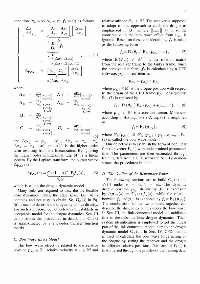
Fig. 12. The grid of the cuboid zone

B. Detailed Procedures of Table III to EstablishFb (·)

Step 1. Setup CFD Environment and Establishthe CFD frame (of − xfyfzf ): Two 3D geometricmodels of the forebody of receiver and the drogueare built in Gambit as shown in Figures 5 and 4. Thecomputational domain is cuboid zone with the sizeof 10×6×6, and the mesh used has about 2.6 millionmixed cells, as shown in Figure 12. To achieve ahigher density, the grid with length about 0.005 isused around the surface of the drogue. The gridlength is 20 times smaller than that near boundaryregion. Standard k-epsilon model is used for airviscous model and the pressure based formulationwith implicit algorithm for the solver. Under thissetting, the pressure on the drogue is acquired byusing the commercial software Fluent.

Then, establish the CFD frame of − xfyfzf forthe CFD tests. In this paper, Fluent is chosen asthe CFD software. As shown in Figure 1, the CFDreference point pf is fixed in xrorzr, and pf withrespect to receiver position pr is denoted by pf/r =[xf/r, yf/r, zf/r

]T. Choose xf/r = xp/r−2.2, yf/r =

0, zf/r = zp/r, where pp/r =[xp/r, yp/r, zp/r

]T ∈ R3

is the probe position with respect to pr. The reasonsto choose such a pf/r are: i) xf/r is at the positionof the cockpit, shown in Figure 1; ii) since yf/r = 0,the element of Fb

(pd/f

)will be either an odd or

an even function about yd/f thanks to the symmetryof the nose; iii) since zf/r = zp/r, the probe alignswith the drogue. Let pf be the original point of ofthe coordinate system in the tests. In the remainderpart of this section, all related variables are definedin the CFD frame. Therefore, for convenience, thesubscript f of the variables measured in of−xfyfzfis omitted. For example, pd = pd/f , xd = xd/f , and

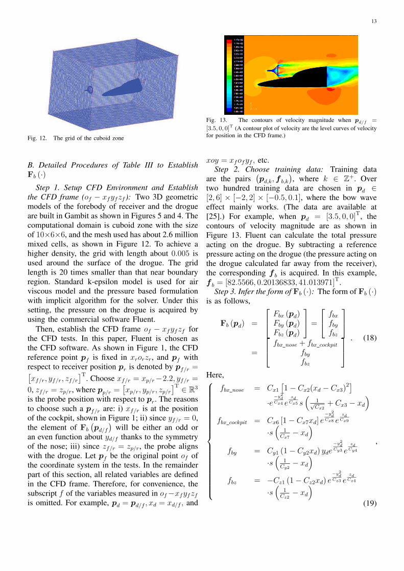
Fig. 13. The contours of velocity magnitude when pd/f =

[3.5, 0, 0]T (A contour plot of velocity are the level curves of velocityfor position in the CFD frame.)

xoy = xfofyf , etc.Step 2. Choose training data: Training data

are the pairs(pd,k,f b,k

), where k ∈ Z+. Over

two hundred training data are chosen in pd ∈[2, 6] × [−2, 2] × [−0.5, 0.1], where the bow waveeffect mainly works. (The data are available at[25].) For example, when pd = [3.5, 0, 0]T, thecontours of velocity magnitude are as shown inFigure 13. Fluent can calculate the total pressureacting on the drogue. By subtracting a referencepressure acting on the drogue (the pressure acting onthe drogue calculated far away from the receiver),the corresponding f b is acquired. In this example,f b = [82.5566, 0.20136833, 41.013971]T.

Step 3. Infer the form of Fb (·): The form of Fb (·)is as follows,

Fb (pd) =

Fbx (pd)Fby (pd)Fbz (pd)

=

fbxfbyfbz

=

fbx nose + fbx cockpit

fbyfbz

. (18)

Here,

fbx nose = Cx1

[1− Cx2(xd − Cx3)

2]·e

−y2dCx4 e

zdCx5 s

(1√Cx2

+ Cx3 − xd

)fbx cockpit = Cx6 [1− Cx7xd] e

−y2dCx8 e

zdCx9

·s(

1Cx7

− xd

)fby = Cy1 (1− Cy2xd) yde

−y2dCy3 e

zdCy4

·s(

1Cy2

− xd

)fbz = −Cz1 (1− Cz2xd) e

−y2dCz3 e

zdCz4

·s(

1Cz2

− xd

)

,

(19)

14

where C(·) > 0 denotes a parameter, and s (·) isdefined in Eq. (14). The process to obtain Eq. (18)is illustrated as follows.

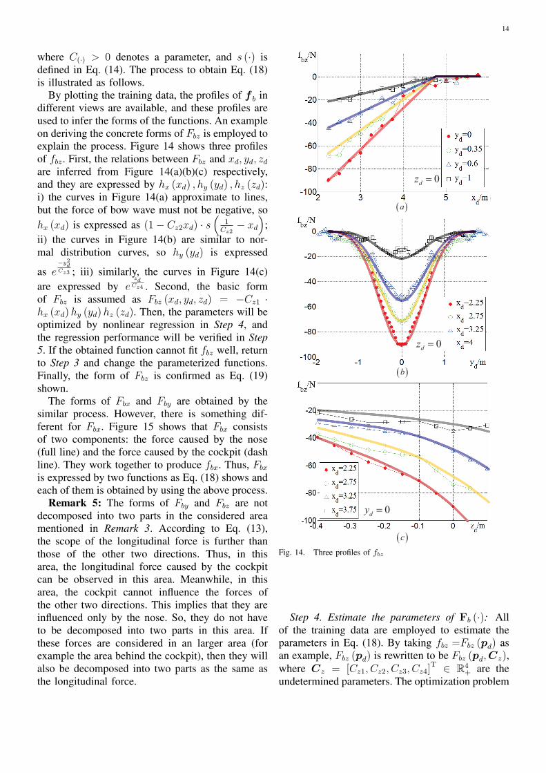
By plotting the training data, the profiles of f b indifferent views are available, and these profiles areused to infer the forms of the functions. An exampleon deriving the concrete forms of Fbz is employed toexplain the process. Figure 14 shows three profilesof fbz. First, the relations between Fbz and xd, yd, zdare inferred from Figure 14(a)(b)(c) respectively,and they are expressed by hx (xd) , hy (yd) , hz (zd):i) the curves in Figure 14(a) approximate to lines,but the force of bow wave must not be negative, sohx (xd) is expressed as (1− Cz2xd) · s

(1

Cz2− xd

);

ii) the curves in Figure 14(b) are similar to nor-mal distribution curves, so hy (yd) is expressed

as e−y2dCz3 ; iii) similarly, the curves in Figure 14(c)

are expressed by ezdCz4 . Second, the basic form

of Fbz is assumed as Fbz (xd, yd, zd) = −Cz1 ·hx (xd)hy (yd)hz (zd). Then, the parameters will beoptimized by nonlinear regression in Step 4, andthe regression performance will be verified in Step5. If the obtained function cannot fit fbz well, returnto Step 3 and change the parameterized functions.Finally, the form of Fbz is confirmed as Eq. (19)shown.

The forms of Fbx and Fby are obtained by thesimilar process. However, there is something dif-ferent for Fbx. Figure 15 shows that Fbx consistsof two components: the force caused by the nose(full line) and the force caused by the cockpit (dashline). They work together to produce fbx. Thus, Fbx

is expressed by two functions as Eq. (18) shows andeach of them is obtained by using the above process.

Remark 5: The forms of Fby and Fbz are notdecomposed into two parts in the considered areamentioned in Remark 3. According to Eq. (13),the scope of the longitudinal force is further thanthose of the other two directions. Thus, in thisarea, the longitudinal force caused by the cockpitcan be observed in this area. Meanwhile, in thisarea, the cockpit cannot influence the forces ofthe other two directions. This implies that they areinfluenced only by the nose. So, they do not haveto be decomposed into two parts in this area. Ifthese forces are considered in an larger area (forexample the area behind the cockpit), then they willalso be decomposed into two parts as the same asthe longitudinal force.

0dz =

0dz =

0dy =

( )a

( )b

( )c

Fig. 14. Three profiles of fbz

Step 4. Estimate the parameters of Fb (·): Allof the training data are employed to estimate theparameters in Eq. (18). By taking fbz =Fbz (pd) asan example, Fbz (pd) is rewritten to be Fbz (pd,Cz),where Cz = [Cz1, Cz2, Cz3, Cz4]

T ∈ R4+ are the

undetermined parameters. The optimization problem

15

Fig. 15. The two components of fbx: the full line caused by thenose and the dash line caused by the cockpit

to find Cz is formulated as follows,

C∗z = argmin

Cz∈R4+

∑N

k=1

[fbz,k − Fbz

(pd,k,Cz

)]2 ,

(20)where N is the number of the training data.The constraint is that all the elements of Cz arepositive. The initial value of Cz is chosen as[170, 0.2, 0.5, 0.6]T, which be estimated by curvefitting in the profiles. As a result, Fbz (pd) =F ′bz (pd,C

∗z). Similarly, the other parameters in Eq.

(18) are determined. The results are shown in Eq.(13).

Step 5. Check regression performance: To checkthe regression performance, the coefficient of de-termination of the regression index R2 is employed[26]. By taking fbz as an example, it follows SSEz =

∑Nk=1

(fbz,k − Fbz

(pd,k,C

∗z

))2SSTz =

∑Nk=1

(fbz,k − 1

N

∑Nk=1 fbz,k

)2 ,

(21)and R2

z = 1 − SSEz

SSTz. By using the training data,

R2x = 0.8866, R2

y = 0.9536, R2z = 0.9671. In gener-

al, if R2 > 0.7, then the regression performance issatisfied. Therefore, it is concluded that the obtainedFb (·) approximates the bow wave force nicely.

REFERENCES

[1] Thomas, P. R., Bhandari U., Bullock S., Richardson, T. S.,du Bois, J. L., “Advances in air to air refuelling”, Progressin Aerospace Sciences, Vol. 71, 2014, pp. 14-35. DOI:10.1016/j.paerosci.2014.07.001

[2] Nalepka, J. P., and Hinchman, J. L., “Automated Aerial Refu-eling: Extending the Effectiveness of Unmanned Air Vehicles,”AIAA Modeling and Simulation Technologies Conference andExhibit, AIAA Paper 2005-6005, San Francisco, Aug. 2005.

[3] Bhandari, U., Thomas, P. R., Bullock, S., Richardson, T. S.,and du Bois, J. K., “Bow Wave Effect in probe-and-drogueAerial Refuelling,” AIAA Guidance, Navigation, and ControlConference, AIAA Paper 2013-4695, Boston, Aug. 2013.

[4] Dogan, A., and Blake, W., “Modeling of Bow Wave Effectin Aerial Refueling,” AIAA Atmospheric Flight MechanicsConference, AIAA Paper 2010-7926, Toronto, Aug. 2010.

[5] NATO, “ATP-56(B) Air-to-Air Refuelling,” Tech. rep., NATO,2010.

[6] Campa, G., Napolitano, M. R., and Fravolini, M. L., “Sim-ulation Environment for Machine Vision Based Aerial Refu-eling for UAVs,” IEEE Transactions on Aerospace and Elec-tronic Systems, Vol. 71, No. 1, 2009, pp. 138-151. DOI:10.1109/TAES.2009.4805269

[7] Khansari-Zadeh, S. M., and Saghafi, F., “Vision-Based Naviga-tion in Autonomous Close Proximity Operations using Neu-ral Networks,” IEEE Transactions on Aerospace and Elec-tronic Systems, Vol. 47, No. 2, 2011, pp. 864-883. DOI:10.1109/TAES.2011.5751231

[8] Hansen, J. L., Murray, J. E., and Campos, N. V., “The NASADryden AAR Project: A Flight Test Approach to an AerialRefueling System,” AIAA Atmospheric Flight Mechanics Con-ference and Exhibit, AIAA Paper 2004-4939, Providence, Aug.2004.

[9] Dibley, R. P., Michael J. Allen, and Dr. Nassib Nabaa, “Au-tonomous Airborne Refueling Demonstration Phase I Flight-Test Results,” AIAA Atmospheric Flight Mechanics Conferenceand Exhibit, AIAA Paper 2007-6639, Hilton Head, Aug. 2007.

[10] Ro, K., Kuk, T., and Kamman, J. W., “Active Control of AerialRefueling Hose-Drogue Systems,” AIAA Guidance, Navigation,and Control Conference, AIAA Paper 2010-8400, Toronto,Aug. 2010.

[11] Dogan, A., Blake, W., and Haag, C., “Bow Wave Effectin Aerial Refueling: Computational Analysis and Modeling,”Journal of Aircraft, Vol. 50, No. 6, 2013, pp. 1856-1868. DOI:10.2514/1.C032165

[12] Khan, O., and Masud, J., “Trajectory Analysis of Basket En-gagement during Aerial Refueling”, AIAA Atmospheric FlightMechanics Conference, AIAA Paper 2014-0190, Maryland,2014.

[13] Ro, K., and Kamman J. W., “Modeling and Simulation of Hose-Paradrogue Aerial Refueling Systems,” Journal of Guidance,Control, and Dynamics, Vol. 33, No. 1, 2010, pp. 53-63. DOI:10.2514/1.45482

[14] Wei, Z.-B., Quan, Q., and Cai, K.-Y., “Research on relationbetween drogue position and interference force for probe-drogue aerial refueling system based on link-connected model,”The 31st Chinese Control Conference, IEEE Paper, Hefei, Jul.2012, pp. 1777-1782. (in Chinese)

[15] Stevens, B. L., Lewis, F. L., Aircraft control and simulation,2nd ed., Wiley, New York, 2003, pp. 4-5.

[16] Dogan, A., Timothy L., and William B., “Wake-Vortex InducedWind with Turbulence in Aerial Refueling—Part A: Flight DataAnalysis,” AIAA Atmospheric Flight Mechanics Conference andExhibit, AIAA Paper 2008-6696, Honolulu, Aug. 2008.

[17] Dogan, A., Timothy L., and William B., “Wake-Vortex InducedWind with Turbulence in Aerial Refueling—Part B: Model andSimulation Validation,” AIAA Atmospheric Flight MechanicsConference and Exhibit, AIAA Paper 2008-6697, Honolulu,Aug. 2008.

[18] Venkataramanan, S., and Dogan, A., “Dynamic effect of trailingvortex with turbulence & time-varying inertia in aerial refu-eling,” AIAA Atmospheric Flight Mechanics Conference andExhibit, AIAA Paper 2004-4945, Providence, Aug. 2004.

[19] Fravolini, M. L., Ficola, A., Napolitano, M. R., Campa G., and

16

Perhinschi, M. G., “Development of modeling and control toolsfor aerial refueling for UAVs,” AIAA Guidance, Navigation,and Control Conference and Exhibit, AIAA Paper 2003-5798,Austin, Aug. 2003.

[20] Tandale, Monish D., Roshawn Bowers, and John Valasek. “Tra-jectory tracking controller for vision-based probe-and-drogueautonomous aerial refueling,” Journal of Guidance, Control,and Dynamics, Vol. 29, No. 4, 2006, pp. 846-857. DOI:10.2514/1.19694

[21] Ro, K., Basaran, E., and Kamman, J. W., “Aerodynamic Char-acteristics of Paradrogue Assembly in an Aerial RefuelingSystem,” Journal of Aircraft, Vol. 44, No. 3, 2007, pp. 963-970. DOI: 10.2514/1.26489

[22] The drogue dynamics under receiver’s bow wave,http://youtu.be/xkWkAlfhUX0.

[23] Vassberg, J. C., Yeh, D. T., Blair, A. J., and Evert, J. M., “Nu-merical Simulations of KC-10 Wing-Mount Aerial RefuelingHose-Drogue Dynamics With A Reel Take-Up System,” 21stApplied Aerodynamics Conference, AIAA Paper 2003-3508,Orlando, Jun. 2003.

[24] Klein, V., Morelli, E. A., Aircraft System Identification: Theoryand Practice, AIAA, Reston, 2006, pp. 395-399.

[25] Wei, Z.-B., Dai, X., Quan, Q., and Cai, K.-Y., “Datasetand Analysis of Bow Wave Effect Based on Fluent”,http://rfly.buaa.edu.cn/resources/#DatasetBowWaveCFD.

[26] Weisberg, S., Applied Linear Regression, 4th ed., Wiley, NewYork, 2005, pp. 33-35.

Zi-Bo Wei is a Ph.D. candidate of School ofAutomation Science and Electrical Engineer-ing at Beihang University (Beijing Universityof Aeronautics and Astronautics). His mainresearch interests are aerial refueling, iterativelearning control and accurate flight control.

Xunhua Dai received the B.S. and M.S. de-grees from School of Automation Science andElectrical Engineering at Beihang Universityin 2013 and 2016, respectively. His main re-search interests are aerial refueling and flyingcontrol.

Quan Quan received the B.S. and Ph.D. de-grees from Beihang University, Beijing, China,in 2004 and 2010, respectively. He has beenan associate professor in Beihang Universitysince 2013. His main research interests includevision-based navigation and reliable flight con-trol.

Kai-Yuan Cai received the B.S., M.S., andPh.D. degrees from Beihang University, Bei-jing, China, in 1984, 1987, and 1991, respec-tively. He has been a full professor at BeihangUniversity since 1995. He is a Cheung KongScholar (chair professor), jointly appointed bythe Ministry of Education of China and the LiKa Shing Foundation of Hong Kong in 1999.His main research interests include software

testing, software reliability, reliable flight control, and software cy-bernetics.