Drawing Game Trees with TikZ - Simon Fraser Universityhaiyunc/notes/Game_Trees_with_TikZ.pdf · 1An...

Drawing Game Trees with TikZ

Haiyun K. Chen∗

Department of Economics, Simon Fraser University

January 7, 2013

Abstract

Game trees, also known as extensive form games, are commonly used to represent

situations of strategic interactions. This document provides examples on how to

produce nice looking game trees in LATEX with the TikZ package.1

Contents

1 Preliminaries 2

2 Drawing Game Trees with TikZ 2

2.1 The tikzpicture Environment . . . . . . . . . . . . . . . . . . . . . . . . . . 2

2.2 Trees in TikZ . . . . . . . . . . . . . . . . . . . . . . . . . . . . . . . . . . . . . 3

2.3 Formatting Nodes . . . . . . . . . . . . . . . . . . . . . . . . . . . . . . . . . . 4

2.4 Information Sets . . . . . . . . . . . . . . . . . . . . . . . . . . . . . . . . . . . 5

2.5 Adding Texts . . . . . . . . . . . . . . . . . . . . . . . . . . . . . . . . . . . . 7

2.6 Formatting Branches . . . . . . . . . . . . . . . . . . . . . . . . . . . . . . . . 8

2.7 Sibling and Level Distances . . . . . . . . . . . . . . . . . . . . . . . . . . . . 9

2.8 Miscellaneous Issues . . . . . . . . . . . . . . . . . . . . . . . . . . . . . . . . 11

2.8.1 Directions of “Growth” . . . . . . . . . . . . . . . . . . . . . . . . . . 11

2.8.2 Automating Text Input . . . . . . . . . . . . . . . . . . . . . . . . . . . 11

∗Comments and suggestions are welcome. Please send them to [email protected] alternative way to draw game trees in LATEX is to use the PSTricks package, and Martin Osborne

has created a style for this purpose (see its documentation for detail).

of 28

http://www.economics.utoronto.ca/osborne/latex/egameps.pdf

http://www.economics.utoronto.ca/osborne/

mailto:[email protected]

http://www.sfu.ca/~haiyunc/

3 Examples 14

3.1 A 2 × 2 Tree with Information Set . . . . . . . . . . . . . . . . . . . . . . . . 14

3.2 Asymmetric Tree . . . . . . . . . . . . . . . . . . . . . . . . . . . . . . . . . . 16

3.3 Sequential-Move Game . . . . . . . . . . . . . . . . . . . . . . . . . . . . . . . 17

3.4 Market Entry Game . . . . . . . . . . . . . . . . . . . . . . . . . . . . . . . . . 19

3.5 Large Information Set . . . . . . . . . . . . . . . . . . . . . . . . . . . . . . . 21

3.6 Centipede Game . . . . . . . . . . . . . . . . . . . . . . . . . . . . . . . . . . 23

3.7 Curved Information Set . . . . . . . . . . . . . . . . . . . . . . . . . . . . . . 25

3.8 Colored and Hybrid Game Tree . . . . . . . . . . . . . . . . . . . . . . . . . . 27

1 Preliminaries

The TikZ package, which comes with standard LATEX distributions. In the preamble, load

the package with:

\usepackage{tikz}

It will be helpful also to use the calc library in TikZ for calculations of coordinates:

\usetikzlibrary{calc}

The coloring of the figures is done through the xcolor package:

\usepackage[dvipsnames]{xcolor}

2 Drawing Game Trees with TikZ

2.1 The tikzpicture Environment

The TikZ commands take effect in the TikZ environment. While there are numerous ways

to introduce the TikZ environment,2 in this article we focus mainly on the tikzpicture

environment, which can be introduced, as other environments in LATEX, with the follow-

ing syntax:

\begin{tikzpicture}[options]

\command_name [options] ... ; % This is a ‘path’ in TikZ.

\end{tikzpicture}

2See the TikZ & PGF Manual for detail.

of 28

http://ctan.mirror.rafal.ca/graphics/pgf/base/doc/generic/pgf/pgfmanual.pdf

A typical path in TikZ generally starts with \command_name, and ends with a semicolon

(;). It is permissible to have multiple commands (or operations, as they are called in the

manual) within a given path. Note, however, for the nested commands (e.g. the second

to fourth node{} command in Figure 1), the “\” sign must be omitted.

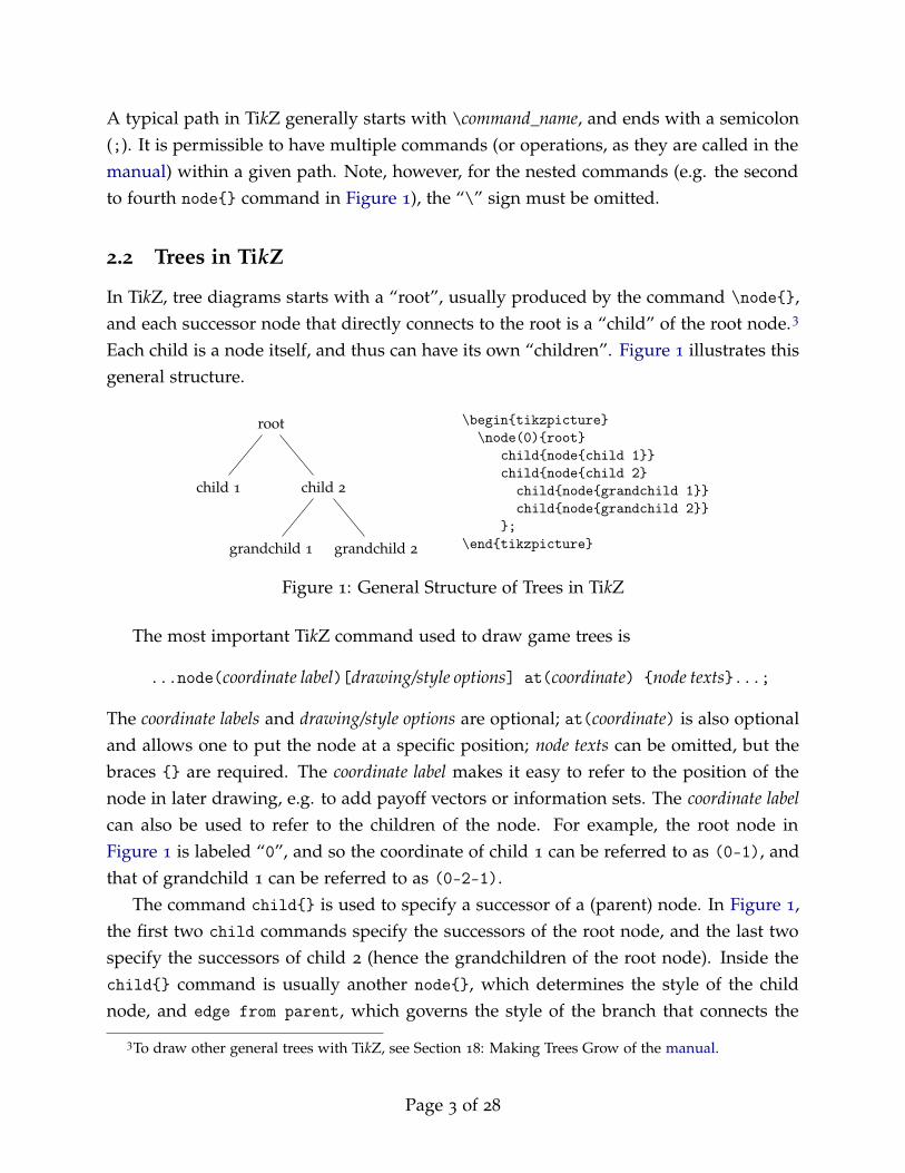
2.2 Trees in TikZ

In TikZ, tree diagrams starts with a “root”, usually produced by the command \node{},

and each successor node that directly connects to the root is a “child” of the root node.3

Each child is a node itself, and thus can have its own “children”. Figure 1 illustrates this

general structure.

root

child 1 child 2

grandchild 1 grandchild 2

\begin{tikzpicture}\node(0){root}

child{node{child 1}}child{node{child 2}child{node{grandchild 1}}child{node{grandchild 2}}

};\end{tikzpicture}

Figure 1: General Structure of Trees in TikZ

The most important TikZ command used to draw game trees is

...node(coordinate label)[drawing/style options] at(coordinate) {node texts}...;

The coordinate labels and drawing/style options are optional; at(coordinate) is also optional

and allows one to put the node at a specific position; node texts can be omitted, but the

braces {} are required. The coordinate label makes it easy to refer to the position of the

node in later drawing, e.g. to add payoff vectors or information sets. The coordinate label

can also be used to refer to the children of the node. For example, the root node in

Figure 1 is labeled “0”, and so the coordinate of child 1 can be referred to as (0-1), and

that of grandchild 1 can be referred to as (0-2-1).

The command child{} is used to specify a successor of a (parent) node. In Figure 1,

the first two child commands specify the successors of the root node, and the last two

specify the successors of child 2 (hence the grandchildren of the root node). Inside the

child{} command is usually another node{}, which determines the style of the child

node, and edge from parent, which governs the style of the branch that connects the

3To draw other general trees with TikZ, see Section 18: Making Trees Grow of the manual.

of 28



child to its parent. Note that if the style of a particular branch needs to be modified,

such as adding texts to the branch or changing its color, edge from parent must be put

after node{} and all of its children.

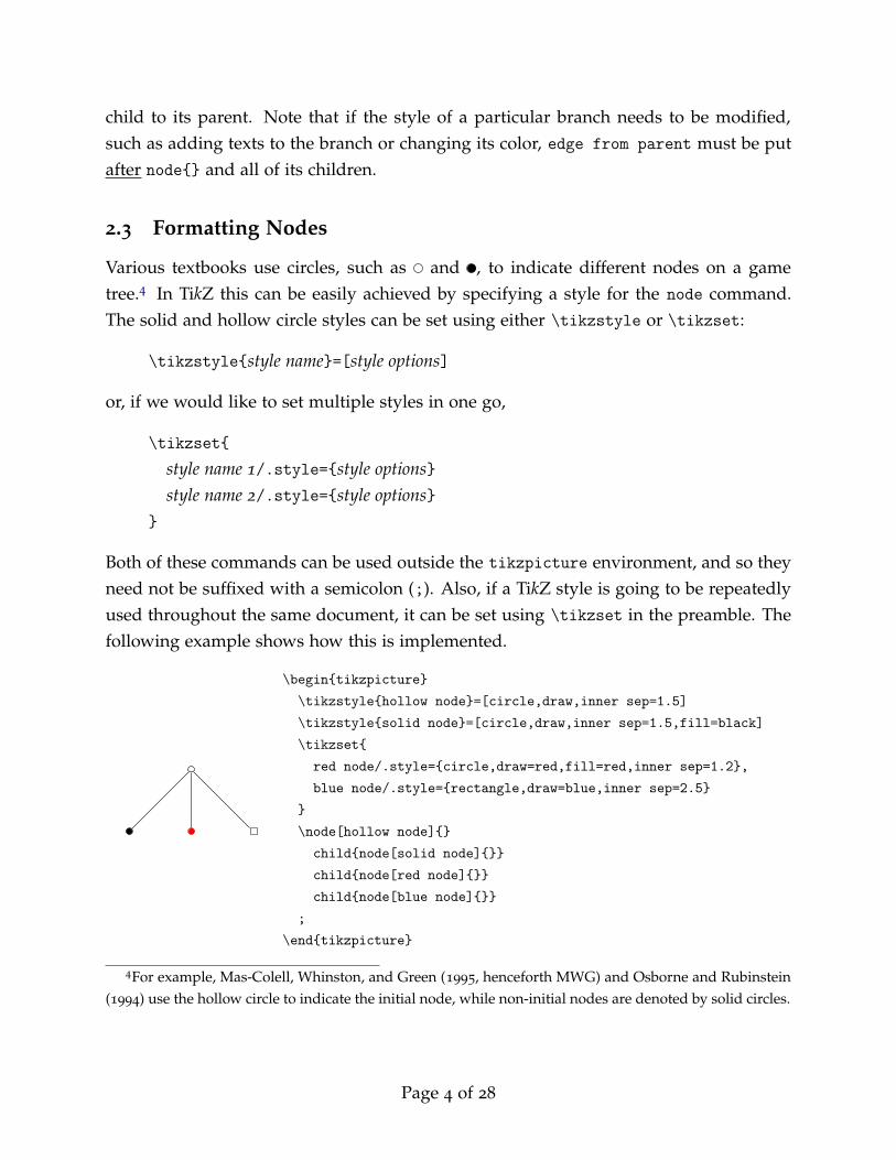
2.3 Formatting Nodes

Various textbooks use circles, such as and , to indicate different nodes on a game

tree.4 In TikZ this can be easily achieved by specifying a style for the node command.

The solid and hollow circle styles can be set using either \tikzstyle or \tikzset:

\tikzstyle{style name}=[style options]

or, if we would like to set multiple styles in one go,

\tikzset{

style name 1/.style={style options}

style name 2/.style={style options}

}

Both of these commands can be used outside the tikzpicture environment, and so they

need not be suffixed with a semicolon (;). Also, if a TikZ style is going to be repeatedly

used throughout the same document, it can be set using \tikzset in the preamble. The

following example shows how this is implemented.

\begin{tikzpicture}

\tikzstyle{hollow node}=[circle,draw,inner sep=1.5]

\tikzstyle{solid node}=[circle,draw,inner sep=1.5,fill=black]

\tikzset{

red node/.style={circle,draw=red,fill=red,inner sep=1.2},

blue node/.style={rectangle,draw=blue,inner sep=2.5}

}

\node[hollow node]{}

child{node[solid node]{}}

child{node[red node]{}}

child{node[blue node]{}}

;

\end{tikzpicture}

4For example, Mas-Colell, Whinston, and Green (1995, henceforth MWG) and Osborne and Rubinstein

(1994) use the hollow circle to indicate the initial node, while non-initial nodes are denoted by solid circles.

of 28

In the code, circle (and rectangle) specifies the shape of a node; draw=color asks TikZ

to draw the boundary of the node with color;5 inner sep=parameter determines—for the

purpose of this article—the size of the node;6 and fill=color fills the interior of a node

with color.

2.4 Information Sets

Information sets in game trees are usually represented as either dashed lines joining

the nodes in an information set ( ), or elongated circles encompassing those nodes

( ). To implement these drawings in TikZ, we can use the \draw command:

\draw[drawing options](coordinate_1) path operation (coordinate_2)

path operation (coordinate_3) ... ;

The coordinates can be referred to using coordinate labels of the node{} command; path

operation allows us to draw, for example, straight lines and curves from one coordinate

to the next (with the operation to), or rectangles with two diagonal angles at coordinate_1

and coordinate_2 (with the rectangle operation). In the following examples, let the initial

node be labeled “0”, so that the coordinate of its ith child (from the left) can be referred

to as (0-i). Here is a simple dash-line information set:

\draw[dashed](0-1)to(0-2)to(0-3);

A curved, dash-line information set:

\draw[dashed,bend right](0-1)to(0-3);

To have more flexible curvature, use the [out=angle,in=angle] option to specify the de-

grees at which the line starts and ends:

5The default color is black, when color is not specified.6In fact, inner sep specifies the space between the texts within a node and its boundary. In the

examples presented in this article, most nodes within a tree will not have textual content. Therefore

inner sep is primarily used to determine the node sizes.

of 28

\draw[dashed,out=45,in=300](0-1)to(0-3);

Color and line style options can easily be added as well:

\draw[dashed,draw=red,line width=2pt]

(0-1)to(0-2)to[out=45,in=300](0-3);

Drawing a “circled” information set is more involved. The idea is to draw a rectangle

(with rounded corners) that encloses the nodes in the same information set. In the \draw

command, we use rectangle as the path operation. Suppose there are two nodes, left and

right, in an information set, with coordinate labels (0-1) and (0-2), respectively. We

want the northwest corner of the rectangle placed above and to the left of the left node,

and the southeast corner placed below and to the right of the right node.7 The positions

of the northwest and southeast corners, to be used as coordinate_1 and coordinate_2 in

the \draw syntax, are relative to the positions of the two nodes. Hence, they can be

calculated as relative coordinates to (0-1) and (0-2).

The calc library provides a method for calculating relative coordinates. Suppose the

position (a1, a2) of a coordinate labeled (A) is known. Then the coordinate (a1 + x, a2 + y)

is given by the syntax: ($(A)+(x,y)$), where x and y are any real numbers.

Therefore, a circled information set can be drawn as follows:

\draw[dashed,rounded corners=7]($(0-1)+(-.25,.25)$)rectangle($(0-2)+(.25,-.25)$);

Figure 2: Game Tree with a Circled Information Set

Here, the rounded corners=parameter determines how “rounded” the corner is.8 Other

drawing options can be added as usual.

Sometimes we may want to circle a single node, e.g. node 0 in Figure 2, to indicate

that it is a singleton (or trivial) information set. This is more easily done using circle as

7Alternatively, we could have the southwest corner of the rectangle positioned below and to the left of

the left node, and the northeast corner above and to the right of the right node.8Depending on the size of the rectangle, the parameter value may have to be manually adjusted.

of 28

the path operation for the \draw command. When drawing a circle, coordinate_1 indicates

the center of the circle and coordinate_2 specifies its radius:

\draw[dashed](0)circle(.25cm);

\draw[dashed,rounded corners=7]

($(0-1)+(-.25,.25)$)rectangle($(0-2)+(.25,-.25)$);

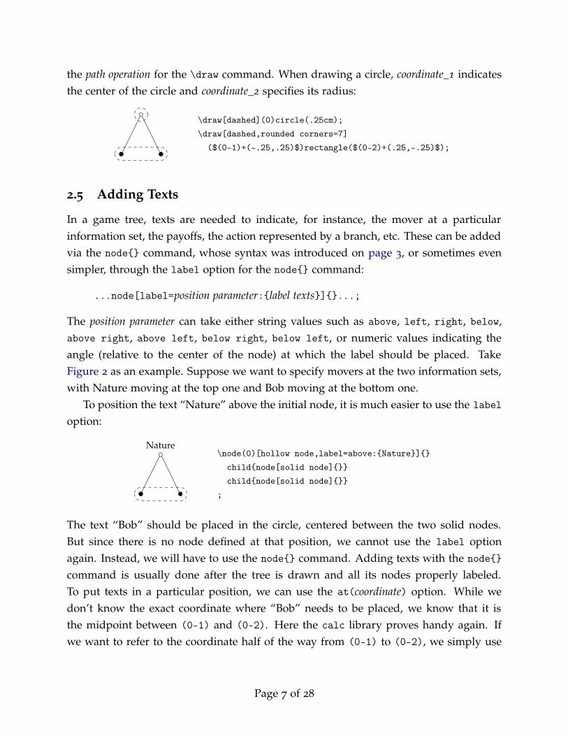
2.5 Adding Texts

In a game tree, texts are needed to indicate, for instance, the mover at a particular

information set, the payoffs, the action represented by a branch, etc. These can be added

via the node{} command, whose syntax was introduced on page 3, or sometimes even

simpler, through the label option for the node{} command:

...node[label=position parameter:{label texts}]{}...;

The position parameter can take either string values such as above, left, right, below,

above right, above left, below right, below left, or numeric values indicating the

angle (relative to the center of the node) at which the label should be placed. Take

Figure 2 as an example. Suppose we want to specify movers at the two information sets,

with Nature moving at the top one and Bob moving at the bottom one.

To position the text “Nature” above the initial node, it is much easier to use the label

option:

Nature\node(0)[hollow node,label=above:{Nature}]{}



;

The text “Bob” should be placed in the circle, centered between the two solid nodes.

But since there is no node defined at that position, we cannot use the label option

again. Instead, we will have to use the node{} command. Adding texts with the node{}

command is usually done after the tree is drawn and all its nodes properly labeled.

To put texts in a particular position, we can use the at(coordinate) option. While we

don’t know the exact coordinate where “Bob” needs to be placed, we know that it is

the midpoint between (0-1) and (0-2). Here the calc library proves handy again. If

we want to refer to the coordinate half of the way from (0-1) to (0-2), we simply use

of 28

($(0-1)!.5!(0-2)$).9 As an aside, we can also see how “Nature” can be added using

node{}:

Nature

Bob

\node(0)[hollow node]{}



;

\node[above]at(0){Nature};

\node at($(0-1)!.5!(0-2)$){Bob};

Notice that the option [above] is given to indicate that “Nature” is above point (0).

Other position options are similar to those used in the label option. Two very useful

position options are worth mentioning: xshift=parameter and yshift=parameter. These

options allows one to shift the node position horizontally and vertically by any unit, and

so are particularly useful when fine-tuning the figure.

Other texts such as payoff vectors can be added similarly. The next subsection goes

over how to format and to add texts to the branches.

2.6 Formatting Branches

The style/formatting of the branches is controlled through edge from parent[options],

which should be put as a second operation of child{}—the first operation should be

node{}.10 The basic options are more or less the same as those for \draw. Texts are

added using a second node{} command, after edge from parent.11 The next example

illustrates how branches can be decorated:9The !.5! in the example could be replaced with other numbers as well. For instance, !.75!

would give the coordinate three quarters on the way from (0-1) to (0-2). To find the mid-

point between two coordinates, we could alternatively use ($.5*(0-1)+.5*(0-2)$), a syntax con-

sistent with the one used in Figure 2. Still another method is to use the [midway] option of

node{} in conjunction with \draw. To put “Bob” in the right place, we could instead have used

\draw[draw=none](0-1)to(0-2) node[midway]{Bob};. The [draw=none] option basically tells TikZ to

draw an invisible line, and the [midway] option puts a node in the middle of this invisible path.10Note that it is not necessary to separate the two operations with anything.11Unfortunately the label option does not work with edge from parent. So branch texts must be

added using node{}.

of 28

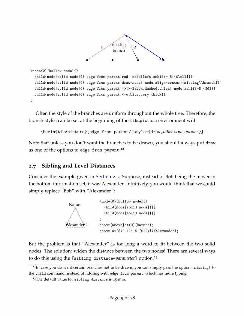
`missing

branchd


child{node[solid node]{} edge from parent[red] node[left,xshift=-5]{$\ell$}}

child{node[solid node]{} edge from parent[draw=none] node[align=center]{missing\\branch}}

child{node[solid node]{} edge from parent[->,>=latex,dashed,thick] node[xshift=8]{$d$}}

child{node[solid node]{} edge from parent[<-o,blue,very thick]}

;

Often the style of the branches are uniform throughout the whole tree. Therefore, the

branch styles can be set at the beginning of the tikzpicture environment with

\begin{tikzpicture}[edge from parent/.style={draw,other style options}]

Note that unless you don’t want the branches to be drawn, you should always put draw

as one of the options to edge from parent.12

2.7 Sibling and Level Distances

Consider the example given in Section 2.5. Suppose, instead of Bob being the mover in

the bottom information set, it was Alexander. Intuitively, you would think that we could

simply replace “Bob” with “Alexander”:

Nature

Alexander




;


\node at($(0-1)!.5!(0-2)$){Alexander};

But the problem is that “Alexander” is too long a word to fit between the two solid

nodes. The solution: widen the distance between the two nodes! There are several ways

to do this using the [sibling distance=parameter] option.13

12In case you do want certain branches not to be drawn, you can simply pass the option [missing] to

the child command, instead of fiddling with edge from parent, which has more typing.13The default value for sibling distance is 15 mm.

of 28

Method 1. Give the [sibling distance=parameter] option to each child{}:

Nature

Alexander


child[sibling distance=25mm]{node[solid node]{}}

child[sibling distance=25mm]{node[solid node]{}}

;



Method 2. Use the option before the first child{} command:

Nature

Alexander


[sibling distance=25mm]



;



Method 3. Specify a level style:

Nature

Alexander

\tikzstyle{level 1}=[sibling distance=25mm]




;



A level style applies to all nodes in a particular level. Using the language in Figure 1,

all children of the root node are level 1 nodes, and all grandchildren are level 2 nodes.

Using the third method is, personally speaking, preferred, as it maintains a uniformity

of style across all nodes in the same level. Moreover, one can always override the level

style by giving options to any particular child{}, as exemplified in Method 1.

In addition to sibling distance, one can also specify level distance in a similar

manner.14

14The default for level distance is also 15 mm.

of 28

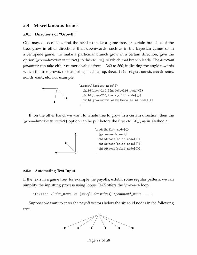
2.8 Miscellaneous Issues

2.8.1 Directions of “Growth”

One may, on occasion, find the need to make a game tree, or certain branches of the

tree, grow in other directions than downwards, such as in the Bayesian games or in

a centipede game. To make a particular branch grow in a certain direction, give the

option [grow=direction parameter] to the child{} to which that branch leads. The direction

parameter can take either numeric values from −360 to 360, indicating the angle towards

which the tree grows, or text strings such as up, down, left, right, north, south west,

north east, etc. For example,


child[grow=left]{node[solid node]{}}

child[grow=260]{node[solid node]{}}

child[grow=south east]{node[solid node]{}}

;

If, on the other hand, we want to whole tree to grow in a certain direction, then the

[grow=direction parameter] option can be put before the first child{}, as in Method 2:

\node[hollow node]{}

[grow=north west]




;

2.8.2 Automating Text Input

If the texts in a game tree, for example the payoffs, exhibit some regular pattern, we can

simplify the inputting process using loops. TikZ offers the \foreach loop:

\foreach \index_name in {set of index values} \command_name ... ;

Suppose we want to enter the payoff vectors below the six solid nodes in the following

tree:

of 28

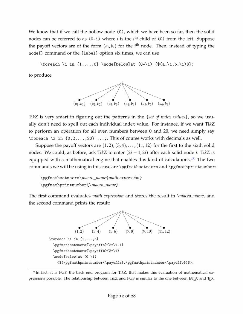
We know that if we call the hollow node (0), which we have been so far, then the solid

nodes can be referred to as (0-i) where i is the ith child of (0) from the left. Suppose

the payoff vectors are of the form (ai, bi) for the ith node. Then, instead of typing the

node{} command or the [label] option six times, we can use

\foreach \i in {1,...,6} \node[below]at (0-\i) {$(a_\i,b_\i)$};

to produce

(a1, b1) (a2, b2) (a3, b3) (a4, b4) (a5, b5) (a6, b6)

TikZ is very smart in figuring out the patterns in the {set of index values}, so we usu-

ally don’t need to spell out each individual index value. For instance, if we want TikZ

to perform an operation for all even numbers between 0 and 20, we need simply say

\foreach \x in {0,2,...,20} ...;. This of course works with decimals as well.

Suppose the payoff vectors are (1, 2), (3, 4), . . . , (11, 12) for the first to the sixth solid

nodes. We could, as before, ask TikZ to enter (2i − 1, 2i) after each solid node i. TikZ is

equipped with a mathematical engine that enables this kind of calculations.15 The two

commands we will be using in this case are \pgfmathsetmacro and \pgfmathprintnumber:

\pgfmathsetmacro\macro_name{math expression}

\pgfmathprintnumber{\macro_name}

The first command evaluates math expression and stores the result in \macro_name, and

the second command prints the result:

(1, 2) (3, 4) (5, 6) (7, 8) (9, 10) (11, 12)

\foreach \i in {1,...,6}

\pgfmathsetmacro{\payoffa}{2*\i-1}

\pgfmathsetmacro{\payoffb}{2*\i}

\node[below]at (0-\i)

{$(\pgfmathprintnumber{\payoffa},\pgfmathprintnumber{\payoffb})$};

15In fact, it is PGF, the back end program for TikZ, that makes this evaluation of mathematical ex-

pressions possible. The relationship between TikZ and PGF is similar to the one between LATEX and TEX.

of 28

Alternatively, we can use the counter function in LATEX to accomplish the same goal:

(1, 2) (3, 4) (5, 6) (7, 8) (9, 10) (11, 12)

\newcounter{payoff}


\node[below]at (0-\i){

$(\stepcounter{payoff}\arabic{payoff},\stepcounter{payoff}\arabic{payoff})$

};

The first line of the code initiates a new counter called payoff.16 In the fourth line,

\stepcounter{payoff} increases the counter payoff by one, and \arabic{payoff} prints

the counter value in Arabic numerals. Instead of numbers, one could also use \alph{}

or \Alph{} to print lower- and upper-case latin alphabets:

(a, B) (c, D) (e, F) (g, H) (i, J) (k, L)

\newcounter{alphpay}


\node[below]at (0-\i){

$(\stepcounter{alphpay}\alph{alphpay},\stepcounter{alphpay}\Alph{alphpay})$

};

16The initial value of all new counters is automatically set to zero. To change this initial value to some

other value, use \setcounter{counter_name}{new_value}.

of 28

3 Examples

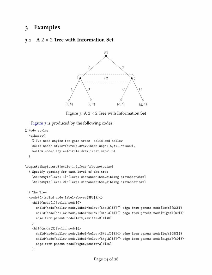
3.1 A 2 × 2 Tree with Information Set

P1

(a, b)

C

(c, d)

D

A

(e, f )

C

(g, h)

D

B

P2

Figure 3: A 2 × 2 Tree with Information Set

Figure 3 is produced by the following codes:

% Node styles

\tikzset{

% Two node styles for game trees: solid and hollow

solid node/.style={circle,draw,inner sep=1.5,fill=black},

hollow node/.style={circle,draw,inner sep=1.5}

}

\begin{tikzpicture}[scale=1.5,font=\footnotesize]

% Specify spacing for each level of the tree

\tikzstyle{level 1}=[level distance=15mm,sibling distance=35mm]


% The Tree

\node(0)[solid node,label=above:{$P1$}]{}

child{node(1)[solid node]{}

child{node[hollow node,label=below:{$(a,b)$}]{} edge from parent node[left]{$C$}}

child{node[hollow node,label=below:{$(c,d)$}]{} edge from parent node[right]{$D$}}

edge from parent node[left,xshift=-3]{$A$}

}


child{node[hollow node,label=below:{$(e,f)$}]{} edge from parent node[left]{$C$}}

child{node[hollow node,label=below:{$(g,h)$}]{} edge from parent node[right]{$D$}}

edge from parent node[right,xshift=3]{$B$}

};

of 28

% information set

\draw[dashed,rounded corners=10]($(1) + (-.2,.25)$)rectangle($(2) +(.2,-.25)$);

% specify mover at 2nd information set

\node at ($(1)!.5!(2)$) {$P2$};

\end{tikzpicture}

This example exhibits several features:

1. It shows how node styles can be set outside of a tikzpicture environment.

2. A TikZ picture can be scaled by giving the option scale=factor to the tikzpicture

environment.

3. Fonts within a TikZ picture can be changed using the font={attribute 1, attribute

2, ...} option. When there is only one attribute, the braces {} are not required.

of 28

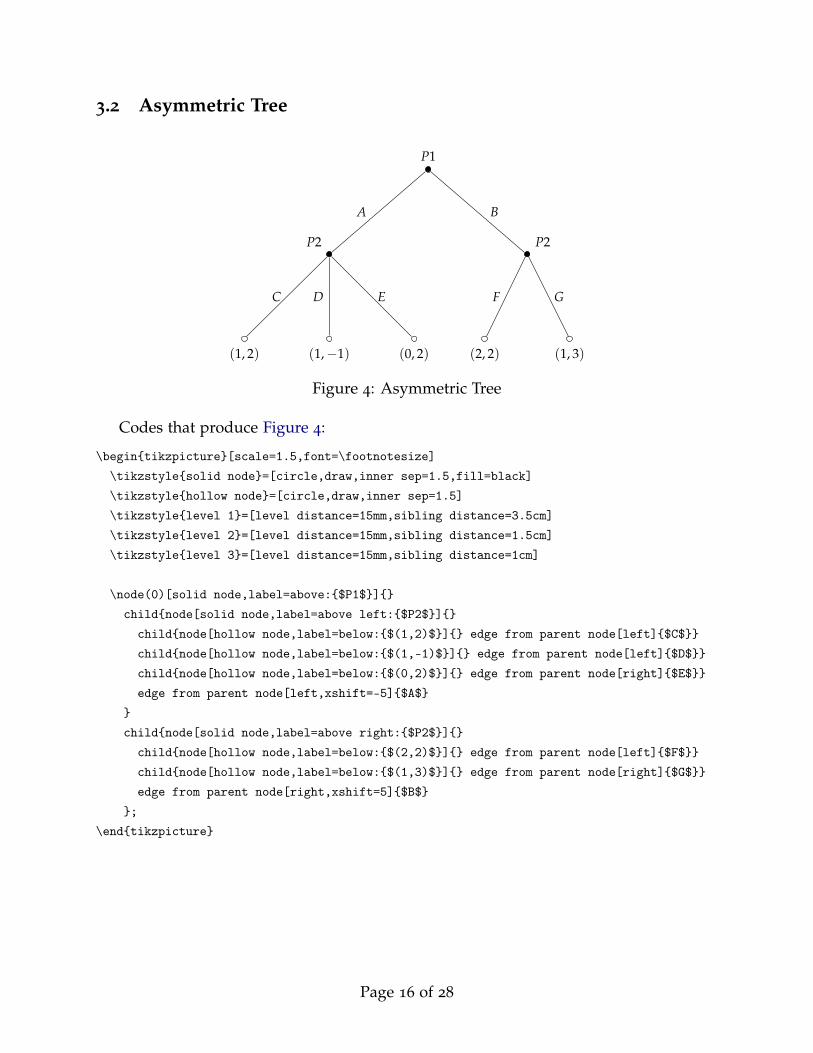
3.2 Asymmetric Tree

P1

P2

(1, 2)

C

(1,−1)

D

(0, 2)

E

A

P2

(2, 2)

F

(1, 3)

G

B

Figure 4: Asymmetric Tree

Codes that produce Figure 4:

\begin{tikzpicture}[scale=1.5,font=\footnotesize]

\tikzstyle{solid node}=[circle,draw,inner sep=1.5,fill=black]

\tikzstyle{hollow node}=[circle,draw,inner sep=1.5]

\tikzstyle{level 1}=[level distance=15mm,sibling distance=3.5cm]

\tikzstyle{level 2}=[level distance=15mm,sibling distance=1.5cm]

\tikzstyle{level 3}=[level distance=15mm,sibling distance=1cm]

\node(0)[solid node,label=above:{$P1$}]{}

child{node[solid node,label=above left:{$P2$}]{}

child{node[hollow node,label=below:{$(1,2)$}]{} edge from parent node[left]{$C$}}

child{node[hollow node,label=below:{$(1,-1)$}]{} edge from parent node[left]{$D$}}

child{node[hollow node,label=below:{$(0,2)$}]{} edge from parent node[right]{$E$}}

edge from parent node[left,xshift=-5]{$A$}

}

child{node[solid node,label=above right:{$P2$}]{}

child{node[hollow node,label=below:{$(2,2)$}]{} edge from parent node[left]{$F$}}

child{node[hollow node,label=below:{$(1,3)$}]{} edge from parent node[right]{$G$}}

edge from parent node[right,xshift=5]{$B$}

};

\end{tikzpicture}

of 28

3.3 Sequential-Move Game

F G

D

F G

E

A

H I J

B

CP1

P1

P2

P2

(a, b) (c, d) (e, f ) (g, h) (i, j) (k, `) (m, n)

(p, q)

Figure 5: Asymmetric, Sequential-Move Game Tree with Information Set


% macro for inputing payoff vectors

\newcommand{\payoff}[4][below]{\node[#1]at(#2){$(#3,#4)$};}

%

\begin{tikzpicture}[scale=1,font=\footnotesize]

% Two node styles: solid and hollow

\tikzstyle{solid node}=[circle,draw,inner sep=1.2,fill=black];

\tikzstyle{hollow node}=[circle,draw,inner sep=1.2];





% The Tree

\node(0)[solid node]{}


child{node[solid node]{}

child{node[hollow node]{}edge from parent node[left]{$F$}}

child{node[hollow node]{}edge from parent node[right]{$G$}}

edge from parent node[left]{$D$}

}


child{node[hollow node]{}edge from parent node[left]{$F$}}

child{node[hollow node]{}edge from parent node[right]{$G$}}

edge from parent node[right]{$E$}

}

edge from parent node[above left]{$A$}

}

of 28

child[missing]

child[level distance=30mm,sibling distance=25mm]{node[solid node]{}

[every child/.style={sibling distance=11mm}]

child{node[hollow node]{}edge from parent node[left]{$H$}}

child{node[hollow node]{}edge from parent node[left]{$I$}}

child{node[hollow node]{}edge from parent node[right]{$J$}}

edge from parent node[above right]{$B$}

}

child[grow=right,level distance=30mm]{node[hollow node]{}

edge from parent node[above]{$C$}

};

% information set

\draw[dashed,rounded corners=7]($(1-1)+(-.2,.25)$)rectangle($(1-2)+(.2,-.25)$);

% specify movers

\node[above]at(0){$P1$};

\node at ($.5*(1-1)+.5*(1-2)$) {$P1$};

\node[above left]at(1){$P2$};

\node[above right]at(0-3){$P2$};

% payoffs

\payoff{1-1-1}ab

\payoff{1-1-2}cd

\payoff{1-2-1}ef

\payoff{1-2-2}gh

\payoff{0-3-1}ij

\payoff{0-3-2}k{\ell}

\payoff{0-3-3}mn

\payoff[right]{0-4}pq

\end{tikzpicture}

All texts in this example are entered using the \node command after the tree is drawn.

Part of the reason for doing this is to showcase the feature that one can define LATEX

macros that cuts down on the typing.17 Since payoffs in a game tree usually involves

mathematical texts, the macro \payoff in this example saves us the trouble of having to

type, for every payoff vector, the $ signs, the parentheses (), and the comma separating

the players’ payoffs. While this may not seem like a huge reduction in typing, but as

Figure 6 shows, macros can be extremely helpful when the texts to be entered have a

certain pattern.

17See Wikibooks’ introduction on how to define and use LATEX macros.

of 28

http://en.wikibooks.org/wiki/LaTeX/Macros

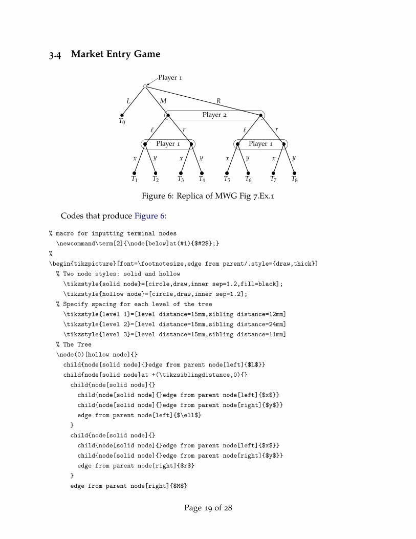
3.4 Market Entry Game

L

x y

`

x y

r

M

x y

`

x y

r

R

Player 1

Player 2

Player 1 Player 1

T0

T1 T2 T3 T4 T5 T6 T7 T8

Figure 6: Replica of MWG Fig 7.Ex.1


% macro for inputting terminal nodes

\newcommand\term[2]{\node[below]at(#1){$#2$};}

%

\begin{tikzpicture}[font=\footnotesize,edge from parent/.style={draw,thick}]








% The Tree


child{node[solid node]{}edge from parent node[left]{$L$}}

child{node[solid node]at +(\tikzsiblingdistance,0){}


child{node[solid node]{}edge from parent node[left]{$x$}}

child{node[solid node]{}edge from parent node[right]{$y$}}

edge from parent node[left]{$\ell$}

}




edge from parent node[right]{$r$}

}

edge from parent node[right]{$M$}

of 28

}

child[sibling distance=5*\tikzsiblingdistance]{node[solid node]{}




edge from parent node[left]{$\ell$}

}




edge from parent node[right]{$r$}

}

edge from parent node[right,xshift=15]{$R$}

};

% information sets

\draw[rounded corners=7]($(0-2)+(-.2,.25)$)rectangle($(0-3)+(.2,-.25)$);

\draw[rounded corners=7]($(0-2-1)+(-.2,.25)$)rectangle($(0-2-2)+(.2,-.25)$);

\draw[rounded corners=7]($(0-3-1)+(-.2,.25)$)rectangle($(0-3-2)+(.2,-.25)$);

% specifying movers

\draw[draw,<-,>=latex](0)--(32:8mm)node[right,inner sep=0]{Player 1};

\node at ($.5*(0-2)+.5*(0-3)$) {Player 2};

\node at ($.5*(0-2-1)+.5*(0-2-2)$) {Player 1};

\node at ($.5*(0-3-1)+.5*(0-3-2)$) {Player 1};

% specifying terminal nodes

\newcounter{tnode}

\setcounter{tnode}{0}

\term{0-1}{T_\arabic{tnode}}

\foreach \x in {2,3}

\foreach \y in {1,2}

\foreach \z in {1,2}

\stepcounter{tnode}

\term{0-\x-\y-\z}{T_\arabic{tnode}};

\end{tikzpicture}

of 28

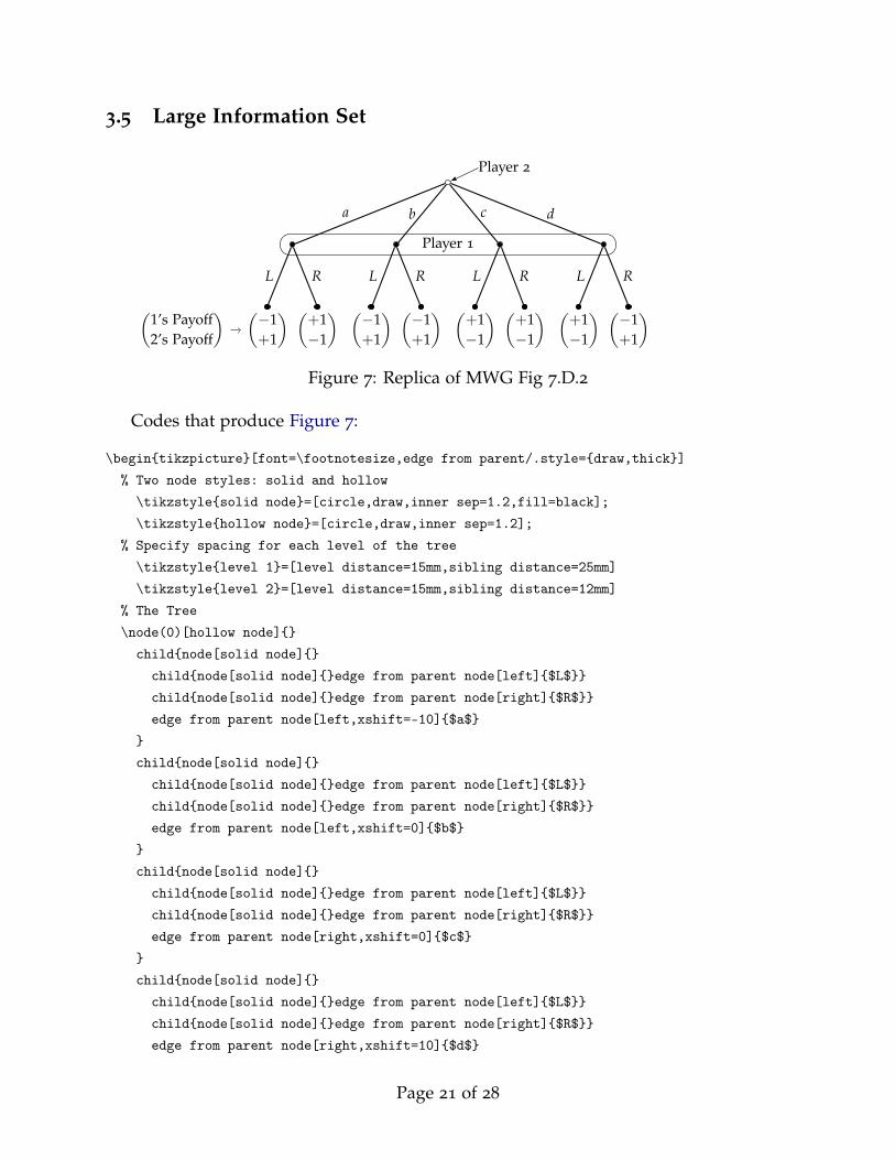
3.5 Large Information Set

L R

a

L R

b

L R

c

L R

d

Player 2

Player 1

(−1+1

) (+1−1

) (−1+1

) (−1+1

) (+1−1

) (+1−1

) (+1−1

) (−1+1

)(1’s Payoff2’s Payoff

)

Figure 7: Replica of MWG Fig 7.D.2









% The Tree




child{node[solid node]{}edge from parent node[right]{$R$}}

edge from parent node[left,xshift=-10]{$a$}

}




edge from parent node[left,xshift=0]{$b$}

}




edge from parent node[right,xshift=0]{$c$}

}




edge from parent node[right,xshift=10]{$d$}

of 28

};

% information set

\draw[rounded corners=7]($(0-1)+(-.3,.25)$)rectangle($(0-4)+(.3,-.25)$);

% specifying movers

\draw[<-,>=latex](0)--(25:8mm)node[inner sep=0,right]{Player 2};

\node at($.5*(0-1)+.5*(0-4)$){Player 1};

% specifying payoffs

\node(payoff)[below]at(0-1-1){$\displaystyle\binom{-1}{+1}$};

\node[below]at(0-1-2){$\displaystyle\binom{+1}{-1}$};

\node[below]at(0-2-1){$\displaystyle\binom{-1}{+1}$};






\draw[<-](payoff)--+(-.9,0)node[left]

{$\displaystyle\binom{\text{$1$’s Payoff}}{\text{$2$’s Payoff}}$};

\end{tikzpicture}

of 28

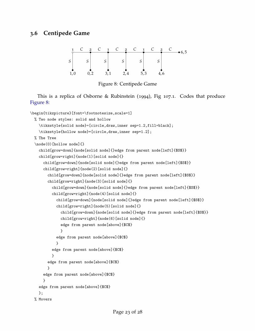
3.6 Centipede Game

S S S S S S

CCCCCC1 1 12 2 2

1, 0 0, 2 3, 1 2, 4 5, 3 4, 6

6, 5

Figure 8: Centipede Game

This is a replica of Osborne & Rubinstein (1994), Fig 107.1. Codes that produceFigure 8:

\begin{tikzpicture}[font=\footnotesize,scale=1]




% The Tree


child[grow=down]{node[solid node]{}edge from parent node[left]{$S$}}

child[grow=right]{node(1)[solid node]{}












}


}


}


}


}


};

% Movers

of 28

\foreach \x in {0,2,4}

\node[above]at(\x){1};

\foreach \x in {1,3,5}

\node[above]at(\x){2};

% payoffs

\node[below]at(0-1){$1,0$};






\node[right]at(6){$6,5$};

\end{tikzpicture}

of 28

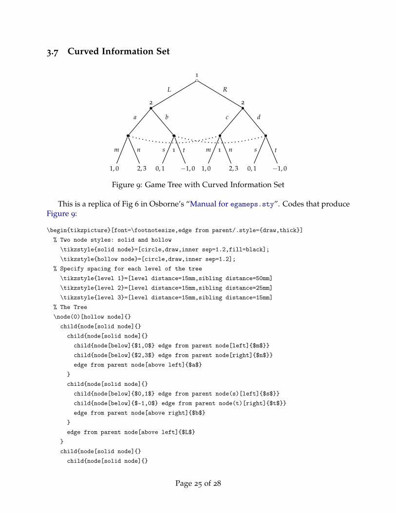
3.7 Curved Information Set

1, 0

m

2, 3

n

a

0, 1

s

−1, 0

t

b

L

1, 0

m

2, 3

n

c

0, 1

s

−1, 0

t

d

R

1

2 2

1 1

Figure 9: Game Tree with Curved Information Set

This is a replica of Fig 6 in Osborne’s “Manual for egameps.sty”. Codes that produceFigure 9:









% The Tree




child{node[below]{$1,0$} edge from parent node[left]{$m$}}

child{node[below]{$2,3$} edge from parent node[right]{$n$}}

edge from parent node[above left]{$a$}

}


child{node[below]{$0,1$} edge from parent node(s)[left]{$s$}}

child{node[below]{$-1,0$} edge from parent node(t)[right]{$t$}}

edge from parent node[above right]{$b$}

}

edge from parent node[above left]{$L$}

}



of 28


child{node[below]{$1,0$} edge from parent node(m)[left]{$m$}}

child{node[below]{$2,3$} edge from parent node(n)[right]{$n$}}

edge from parent node[above left]{$c$}

}


child{node[below]{$0,1$} edge from parent node[left]{$s$}}

child{node[below]{$-1,0$} edge from parent node[right]{$t$}}

edge from parent node[above right]{$d$}

}

edge from parent node[above right]{$R$}

};

% information sets

\draw[loosely dotted,very thick](0-1-1)to[out=-15,in=195](0-2-1);

\draw[loosely dotted,very thick](0-1-2)to[out=-15,in=195](0-2-2);

% movers

\node[above,yshift=2]at(0){1};

\foreach \x in {1,2} \node[above,yshift=2]at(0-\x){2};

\node at($.5*(s)+.5*(t)$){1};

\node at($.5*(m)+.5*(n)$){1};

\end{tikzpicture}

of 28

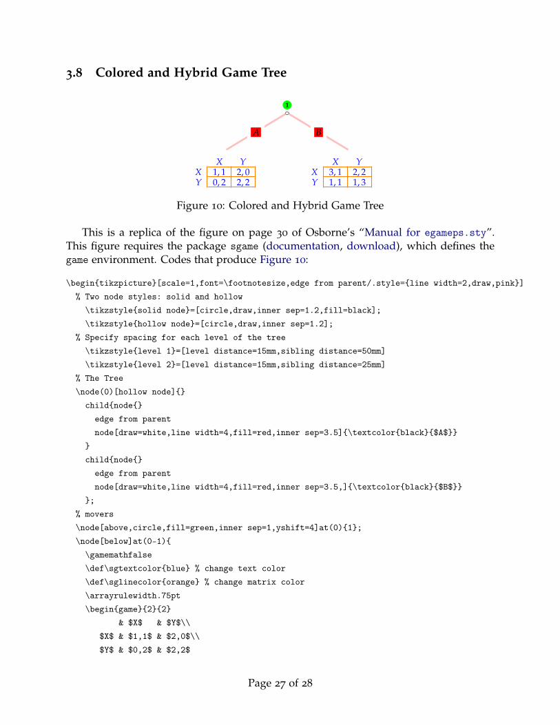
3.8 Colored and Hybrid Game Tree

A B

1

X YX 1, 1 2, 0Y 0, 2 2, 2

X YX 3, 1 2, 2Y 1, 1 1, 3

Figure 10: Colored and Hybrid Game Tree

This is a replica of the figure on page 30 of Osborne’s “Manual for egameps.sty”.This figure requires the package sgame (documentation, download), which defines thegame environment. Codes that produce Figure 10:

\begin{tikzpicture}[scale=1,font=\footnotesize,edge from parent/.style={line width=2,draw,pink}]







% The Tree


child{node{}

edge from parent

node[draw=white,line width=4,fill=red,inner sep=3.5]{\textcolor{black}{$A$}}

}

child{node{}

edge from parent

node[draw=white,line width=4,fill=red,inner sep=3.5,]{\textcolor{black}{$B$}}

};

% movers

\node[above,circle,fill=green,inner sep=1,yshift=4]at(0){1};

\node[below]at(0-1){

\gamemathfalse

\def\sgtextcolor{blue} % change text color

\def\sglinecolor{orange} % change matrix color

\arrayrulewidth.75pt

\begin{game}{2}{2}

& $X$ & $Y$\\

$X$ & $1,1$ & $2,0$\\

$Y$ & $0,2$ & $2,2$

of 28

http://www.economics.utoronto.ca/osborne/latex/sgame.sty

http://www.economics.utoronto.ca/osborne/latex/sgame.pdf


\end{game}

};

\node[below,xshift=-15]at(0-2){

\gamemathfalse

\def\sgtextcolor{blue} % change text color

\def\sglinecolor{orange} % change matrix color

\arrayrulewidth.75pt

\begin{game}{2}{2}

& $X$ & $Y$\\

$X$ & $3,1$ & $2,2$\\

$Y$ & $1,1$ & $1,3$

\end{game}

};

\end{tikzpicture}

of 28

Drawing Game Trees with TikZ - Simon Fraser Universityhaiyunc/notes/Game_Trees_with_TikZ.pdf · 1An...

Documents

Transcript of Drawing Game Trees with TikZ - Simon Fraser Universityhaiyunc/notes/Game_Trees_with_TikZ.pdf · 1An...