Draft Technical Appendix - caiso.com

Flexible Ramping Product

Draft Technical Appendix

June 10, 2015

CAISO/GAA&EMK&CCB June 10, 2015

Table of Contents 1. Introduction ......................................................................................................................... 3

2. Generalized flexible ramping capacity model ...................................................................... 3

3. Flexible ramping product summary ..................................................................................... 5

4. Flexible ramping product objective function ......................................................................... 7

5. Flexible ramping requirement .............................................................................................. 8

5.1 Flexible ramping product total requirement .................................................................. 8

5.2 Flexible ramp requirement due to net demand forecast change ................................... 9

5.3 Flexible ramping requirement due to uncertainty .........................................................10

6. Flexible ramping resource constraints ................................................................................17

6.1 Flexible ramp eligibility constraint ................................................................................17

6.2 Resource ramping capability constraint .......................................................................18

7. Properties of flexible ramping .............................................................................................18

7.1 Upward flexible ramping..............................................................................................19

7.2 Downward flexible ramping .........................................................................................21

8. Settlement ..........................................................................................................................23

9. Cost allocation ...................................................................................................................27

9.1 Proposed movement baseline .....................................................................................27

9.2 Billing determinant of load category ............................................................................29

9.3 Billing determinant of supply category .........................................................................29

9.4 Billing determinant of intertie fixed ramp category .......................................................30

9.5 Monthly re-settlement .................................................................................................30


1. Introduction This technical appendix documents the proposed design for a market-based flexible ramping product (FRP). The ISO is proposing the FRP to maintain power balance in the real-time dispatch and appropriately compensate ramping capability.

The ISO issued a draft final proposal for the FRP on December 4, 2014. Due to stakeholder feedback asking for additional technical details and clarifications, the ISO is issuing this draft technical appendix, which will serve as a supplement to the FRP draft final proposal. The ISO plans to produce a final version of this technical appendix after reviewing with stakeholders. The ISO plans to also revise the draft final proposal that was posted on December 4, 2014 to be consistent.

This draft technical proposal makes the following clarifications and changes to FRP design the December 4, 2014 FRP draft final proposal outlined:

• The ISO will only procure FRP in the real-time market and will not procure FRP in the day-ahead market.

• The portion of FRP the ISO market will procure for uncertainty in the fifteen-minute market will be based on the net load forecast error between the first advisory fifteen-minute market (FMM) interval and the corresponding binding five-minute real-time dispatch (RTD) interval. The portion of FRP the ISO market will procure for uncertainty in RTD will be based on historical net load forecast error between the first advisory RTD interval and the binding RTD interval.

• The ISO made several clarifications and added additional detail to the formulation of the FRP procurement objective function and constraint in the ISO market.

• The ISO made several clarifications and added additional detail to the methodology to procure FRP using a demand curve.

• The ISO will financially settle FRP in the fifteen-minute market and the five-minute market. To reduce implementation complexity, the ISO proposes to simplify its previous proposal for “no-pay” rules that were closely similar to the ancillary services no-pay rules.

2. Generalized flexible ramping capacity model This section gives a brief overview of the flexible ramping capacity model in order to illustrate the flexible ramping procurement concept. For simplicity the ISO does not include any ancillary services below; however, the full model will include ancillary service constraints. Figure 1 shows the potential flexible ramping up and down awards for a resource in time period t that can be procured based on the resource’s ramping capability from t to t+1.


FIGURE 1: SIMPLIFIED FRP ILLUSTRATION OF CONCEPTUAL MODEL

The dashed lines represent the upward and downward ramping capability of the resource from its energy schedule in time period t. The flexible ramping up and down awards are limited by the ramping capability of the resource. The flexible ramping award may also include capacity that is needed to meet the scheduled ramping needs between t and t+1.

Both energy schedules (ENt, ENt+1) and flexible ramp awards (FRUt, FRDt) are calculated simultaneously by the market optimization engine. The only exception is the initial point (EN0) of where the resource is scheduled in t-1, which is a fixed input for the ramp to the resource’s energy schedule in time period t. These control variables are constrained by the following set of capacity and ramp constraints:

max(𝐸𝑁𝑡 + 𝐹𝐹𝐹𝑡,𝐸𝑁𝑡+1) ≤ 𝐹𝐸𝐶𝑡+1min(𝐸𝑁𝑡 + 𝐹𝐹𝐹𝑡,𝐸𝑁𝑡+1) ≥ 𝐶𝐸𝐶𝑡+1𝐹𝐹𝐹(𝐸𝑁𝑡,𝑇) ≤ 𝐹𝐹𝐹𝑡 ≤ 00 ≤ 𝐹𝐹𝐹𝑡 ≤ 𝐹𝐹𝐹(𝐸𝑁𝑡,𝑇)𝐹𝐹𝐹(𝐸𝑁𝑡,𝑇) ≤ 𝐸𝑁𝑡+1 − 𝐸𝑁𝑡 ≤ 𝐹𝐹𝐹(𝐸𝑁𝑡,𝑇)

𝐸𝑁𝑖,𝑡 Energy schedule of Resource i in time period t (positive for supply and negative for demand).

𝐹𝐹𝐹𝑖,𝑡 Flexible Ramp Up award of Resource i in time period t.

𝐹𝐹𝐹𝑖,𝑡 Flexible Ramp Down award (non-positive) of Resource i in time period t.

𝐹𝐸𝐶𝑖,𝑡 Upper Economic Limit of Resource i in time period t.

𝐶𝐸𝐶𝑖,𝑡 Lower Economic Limit of Resource i in time period t.

𝐹𝐹𝐹𝑖(𝐸𝑁,𝑇) Piecewise linear ramp up capability function of Resource i for time interval T.

𝐹𝐹𝐹𝑖(𝐸𝑁,𝑇) Piecewise linear ramp down capability function (non-positive) of Resource i for time interval T.

FRP will help the system to maintain and use dispatchable capacity. It will be dispatched to meet five minute to five minute net system demand changes and will be modeled as a ramping capability constraint. Both the five-minute RTD and fifteen-minute real time unit commitment (RTUC) will schedule FRP throughout their dispatch horizon. Awards will be compensated according to marginal FRP prices in the financially binding RTD interval (the first interval) and in

ENt+1 MW

t t+1

ENt

FRDt

FRUt


the FMM, which is the financially binding RTUC interval (the second interval). Modeling FRP in RTUC enables the market to commit or decommit resources as needed to obtain sufficient upward or downward ramping capability.

3. Flexible ramping product summary The FRP will be procured and dispatched in both the RTD and RTUC using similar methodologies. The FRP is designed with specific constraints and ramping requirements to ensure that there is sufficient ramping capability available in the financially binding five-minute interval to meet the forecasted net load for interval t+5 and cover upwards and downwards forecast error uncertainty. Section 4 – section 6 cover the mathematical representation of these specific constraints and requirements.

In RTD, the FRU and FRD requirements are determined using the forecasted five minute net demand variation. The forecasted net demand variation is made up of (1) the forecasted net load change between the binding and first advisory interval and (2) the highest expected error in the RTD net demand forecast within a 95% confidence interval. Both segments will be procured using a demand curve capped at $247/MW, which is $3/MW less than the ancillary services demand cap. This is described further in section 5.

The probability distribution function for the five minute net demand forecast error is approximated by a histogram constructed from historical observations obtained from consecutive RTD runs over time periods that represents similar real-time conditions. The net load forecast error sample for a given five-minute interval is calculated as the difference between observed net demand for the binding RTD solution for that interval and forecasted net demand for the corresponding advisory interval of the previous RTD run.

Figure 2 illustrates the FRP requirement when net load is ramping upward.

FIGURE 2: FLEXIBLE RAMPING PRODUCT RTD REQUIREMENT ILLUSTATIVE SINGLE INTERVAL EXAMPLE


Figure 3 illustrates how the multi-interval optimization will treat FRP in each subsequent advisory interval in the real-time outlook.1 Each advisory interval will reserve the forecasted net load change between successive advisory intervals and a portion of the predicted net load forecast error uncertainty, using an interval specific demand curve. If the outlook period is within the same hour and therefore the same histogram as the binding interval, the uncertainty portion of the demand curve will be the same in the binding and advisory FRP procurement. Outside the hour, the uncertainty portion of the demand curve may change because the underlying histogram may be different (e.g. the histogram for 8:00am may be different than the histogram for 9:00am.) Therefore, there will be the same uncertainty in each subsequent advisory interval within hour 10:00, but in hour 11:00 the underlying demand curve may change.

The expected net load forecast change will be the difference between each subsequent advisory interval’s and the previous adjacent interval’s net load. The uncertainty for each advisory interval will be calculated using a net demand forecast within a 95% confidence interval procured using a demand curve.

FIGURE 3: FLEXIBLE RAMPING PRODUCT RTD REQUIREMENT ILLUSTATIVE MULTI

INTERVAL EXAMPLE

Figure 4 illustrates RTUC FRP procurement for the binding interval. Similar to RTD, in RTUC the FRU and FRD requirements are determined by the forecasted 15-minute net demand variation. The forecasted net demand variation is made up of (1) the forecasted net load change between the binding and first advisory interval and (2) the highest expected error between the

1 RTD looks out between 9 and 13 intervals.


RTUC first advisory interval and the associated RTD binding interval within a 95% confidence interval.

FIGURE 4: FLEXIBLE RAMPING PRODUCT RTUC REQUIREMENT ILLUSTATIVE EXAMPLE

4. Flexible ramping product objective function This section describes the objective and cost function of the FRP. The FRP will be procured to meet the predicted net demand variation and uncertainty requirements using a demand curve at the cost of expected power balance violations in absence of FRP.

𝐶 = ⋯+ � � 𝐶𝑆𝐹̇ 𝑡(𝐹𝐹𝐹𝑆𝑡) 𝑑𝑟

𝐹𝑅𝑈𝑆𝑡

0

𝑁

𝑡=1

+ � � 𝐶𝑆𝐹̇ 𝑡(𝐹𝐹𝐹𝑆𝑡) 𝑑𝑟

𝐹𝑅𝑃𝑆𝑡

0

𝑁

𝑡=1

A surplus variable is used to determine the expected cost of not procuring a portion of the uncertainty. The FRU/FRD surplus cost function for the flexible ramp requirement due to uncertainty is the expected uncertainty multiplied by the relevant price cap:

𝐶𝑆𝐹𝑡(𝐹𝐹𝐹𝑆𝑡) = 𝑃𝐶 � 𝑟 𝑝𝑡(𝑟) 𝑑𝑟

𝐸𝑈𝑡

𝐸𝑈𝑡−𝐹𝑅𝑈𝑆𝑡

, 0 ≤ 𝐹𝐹𝐹𝑆𝑡 ≤ 𝐹𝐹𝐹𝐹𝑈𝑡

𝐶𝑆𝐹𝑡(𝐹𝐹𝐹𝑆𝑡) = 𝑃𝐹 � 𝑟 𝑝𝑡(𝑟) 𝑑𝑟

𝐸𝑃𝑡−𝐹𝑅𝑃𝑆𝑡

𝐸𝑃𝑡

, 0 ≥ 𝐹𝐹𝐹𝑆𝑡 ≥ 𝐹𝐹𝐹𝐹𝑈𝑡⎭⎪⎪⎬

⎪⎪⎫

, 𝑡 = 1,2, … ,𝑁

And the incremental FRU/FRD surplus cost function is extended to the total flexible ramp


requirement:

𝐶𝑆𝐹̇ 𝑡(𝐹𝐹𝐹𝑆𝑡) = 𝐶𝑆𝐹̇ 𝑡(𝐹𝐹𝐹𝐹𝑈𝑡),𝐹𝐹𝐹𝐹𝑈𝑡 < 𝐹𝐹𝐹𝑆𝑡 ≤ 𝐹𝐹𝐹𝐹𝑡𝐶𝑆𝐹̇ 𝑡(𝐹𝐹𝐹𝑆𝑡) = 𝐶𝑆𝐹̇ 𝑡(𝐹𝐹𝐹𝐹𝑈𝑡),𝐹𝐹𝐹𝐹𝑈𝑡 > 𝐹𝐹𝐹𝑆𝑡 ≥ 𝐹𝐹𝐹𝐹𝑡

� , 𝑡 = 1,2, … ,𝑁

e Average 5min net demand forecast error of portion of uncertainty not procured

𝑝𝑡(𝑟) Probability distribution function for the average 5min net demand forecast error in time period t, approximated by a histogram compiled from historical observations.

𝐹𝐹𝐹𝑆𝑡 Flexible Ramp Up surplus in time period t.

𝐹𝐹𝐹𝑆𝑡 Flexible Ramp Down surplus in time period t.

𝐶𝑆𝐹𝑡(𝐹𝐹𝐹𝑆𝑡) Flexible Ramp Up surplus cost function in time period t.

𝐶𝑆𝐹𝑡(𝐹𝐹𝐹𝑆𝑡) Flexible Ramp Down surplus cost function in time period t.

𝐹𝐹𝐹𝐹𝑈𝑡 Flexible Ramp Up requirement due to uncertainty within specified confidence interval in time period t.

𝐹𝐹𝐹𝐹𝑈𝑡 Flexible Ramp Down requirement due to uncertainty within specified confidence interval in time period t.

C Objective function.

PC Bid Price ceiling, currently $1,000/MWh.

PF Bid Price floor, currently –$150/MWh.

𝐸𝐹𝑡 Flexible Ramp Up uncertainty at the upper confidence level in time period t.

𝐸𝐹𝑡 Flexible Ramp Down uncertainty (negative) at the lower confidence level in time period t.

The cost functions and their derivatives above can be approximated using the relevant histogram compiled from historical observations, leading to a stepwise incremental cost function that must be forced to be monotonically increasing for FRUS and monotonically decreasing for FRDS, as required by market optimization solvers for convergence.

5. Flexible ramping requirement

5.1 Flexible ramping product total requirement The FRP total requirement is calculated as the sum of the net demand forecast change across intervals and an additional amount for uncertainty within a 95% confidence interval. The uncertainty will be determined using historical net demand forecast errors and incorporated into a histogram. The histogram will be used to construct a demand curve that the market will use to procure FRP. The market will enforce FRP requirements in all binding and advisory intervals of the RTD and RTUC runs:

𝐹𝐹𝐹𝐹𝑡 = 𝐹𝐹𝐹𝐹ND𝑡 + 𝐹𝐹𝐹𝐹U𝑡𝐹𝐹𝐹𝐹𝑡 = 𝐹𝐹𝐹𝐹ND𝑡 + 𝐹𝐹𝐹𝐹U𝑡

� , 𝑡 = 1,2, … ,𝑁


𝐹𝐹𝐹𝐹𝑡 Total Flexible Ramp Up requirement in time period t.

𝐹𝐹𝐹𝐹ND𝑡 Flexible Ramp Up requirement due to net demand forecast change in time period t.

𝐹𝐹𝐹𝐹U𝑡 Flexible Ramp Up requirement due to uncertainty within specified confidence interval in time period t.

𝐹𝐹𝐹𝐹𝑡 Total Flexible Ramp Down requirement (non-positive) in time period t.

𝐹𝐹𝐹𝐹ND𝑡 Flexible Ramp Down requirement (non-positive) due to net demand forecast change in time period t.

𝐹𝐹𝐹𝐹U𝑡 Flexible Ramp Down requirement due to uncertainty within specified confidence interval in time period t.

5.2 Flexible ramp requirement due to net demand forecast change The minimum FRP is the forecasted real ramping need between intervals. For each binding interval, the market will use the requirement below to procure enough flexible ramping need to meet the forecasted net demand in the next advisory interval. Below is the mathematical representation of the minimum ramping requirement.

The flexible ramp requirement due to net demand forecast change exists only in the direction the net demand forecast is changing; it is zero in the opposite direction:

𝐹𝐹𝐹𝐹ND𝑡 = max(0,∆𝑁𝐹𝑡)𝐹𝐹𝐹𝐹ND𝑡 = min(0,∆𝑁𝐹𝑡)

� , 𝑡 = 1,2, … ,𝑁

𝐖𝐖𝐖𝐖𝐖: ∆NDt = 𝑁𝐹𝑡+1 − 𝑁𝐹𝑡 and 𝑡 = −1 is the initial condition


𝐹𝐹𝐹𝐹𝑈𝑡 Flexible Ramp Down requirement due to uncertainty within specified confidence interval in time period t.

𝑁𝐹𝑡 Net demand forecast in time period t.

The ISO market will only set a FRU or FRD minimum requirement in the event that the forecasted net demand is moving in the same direction as the up or down requirement. Therefore, when the net demand is ramping upward there will not be a minimum FRD requirement, and vice versa. Figure shows an illustrative example of a minimum FRU requirement. In this situation, there is no minimum FRD requirement.


FIGURE 5: FLEXIBLE RAMPING PRODUCT MINIMUM REQUIREMENTS

5.3 Flexible ramping requirement due to uncertainty The ISO market will procure additional flexible capacity using demand curve based on net demand forecast uncertainty. If the supply price is lower, FRP will be procured closer to the maximum ramping requirement. If the supply price is higher, FRP will be procured closer to the minimum requirement.

The flexible ramp requirement due to uncertainty is calculated as follows:

𝐹𝐹𝐹𝐹𝑈𝑡 = max(0,𝐸𝐹𝑡 + 𝐹𝐹𝐹𝐹ND𝑡)𝐹𝐹𝐹𝐹𝑈𝑡 = min(0,𝐸𝐹𝑡 + 𝐹𝐹𝐹𝐹ND𝑡)

� , 𝑡 = 1,2, … ,𝑁

Where:

𝐸𝐹𝑡 = max(0,𝑃𝐹𝑡)

� 𝑝𝑡(𝜀) 𝑑𝜀

𝑃𝑈𝑡

−∞

= 𝐶𝐶𝐹⎭⎬

⎫, 𝑡 = 1,2, … ,𝑁

𝐸𝐹𝑡 = min(0,𝑃𝐹𝑡)

� 𝑝𝑡(𝜀) 𝑑𝜀

𝑃𝑃𝑡

−∞

= 𝐶𝐶𝐹⎭⎬

⎫, 𝑡 = 1,2, … ,𝑁

𝐹𝐹𝐹𝐹U𝑡 Flexible Ramp Up requirement due to uncertainty within specified confidence interval in time period t.

𝐹𝐹𝐹𝐹U𝑡 Flexible Ramp Down requirement due to uncertainty within specified confidence interval in time period t.



𝐹𝐹𝐹𝐹ND𝑡 Flexible Ramp Down requirement (non-positive) due to net demand forecast change in time period t.

𝐸𝐹𝑡 Flexible Ramp Up uncertainty at the upper confidence level in time period t.

𝐸𝐹𝑡 Flexible Ramp Down uncertainty (negative) at the lower confidence level in time period t.

𝑝𝑡(𝜀) Probability distribution function for the average five minute net demand forecast error in time period t, approximated by a histogram compiled from historical observations.

𝑃𝐹𝑡 Cumulative probability of net demand forecast error at or below the upper confidence level in time period t.

𝑃𝐹𝑡 Cumulative probability of net demand forecast error at or below the lower confidence level in time period t.

𝐶𝐶𝐹 Flexible ramp uncertainty upper confidence level, e.g., 97.5%.

𝐶𝐶𝐹 Flexible ramp uncertainty lower confidence level, e.g., 2.5%.

The above formula is illustrated in Figure 5 and Figure 6.

The following formulization shows that the respective FRU and FRD minimum requirements FRP plus the respective FRU and FRD demand curve requirements will equal the respective FRU and FRD total requirements.

�𝐹𝐹𝐹𝑖,𝑡𝑖

+ 𝐹𝐹𝐹𝑆𝑡 = 𝐹𝐹𝐹𝐹𝑡

�𝐹𝐹𝐹𝑖,𝑡𝑖

+ 𝐹𝐹𝐹𝑆𝑡 = 𝐹𝐹𝐹𝐹𝑡⎭⎪⎬

⎪⎫

, 𝑡 = 1,2, … ,𝑁

The surplus variable, i.e. the amount of FRP procured to meet uncertainty evaluated in the model, will be bounded by 0 and the total FRP requirement.

0 ≤ 𝐹𝐹𝐹𝑆𝑡 ≤ 𝐹𝐹𝐹𝐹𝑡 0 ≥ 𝐹𝐹𝐹𝑆𝑡 ≥ 𝐹𝐹𝐹𝐹𝑡

� , 𝑡 = 1,2, … ,𝑁

𝐹𝐹𝐹𝐹𝑡 Total Flexible Ramp Up requirement in time period t.

𝐹𝐹𝐹𝐹𝑡 Total Flexible Ramp Down requirement (non-positive) in time period t.

𝐹𝐹𝐹𝑆𝑡 Flexible Ramp Up surplus in time period t.

𝐹𝐹𝐹𝑆𝑡 Flexible Ramp Down surplus (non-positive) in time period t.




The market will only procure the uncertainty portion of the FRD requirement if the uncertainty is greater than the FRU requirement due to net demand forecast change.

FIGURE 5: FLEXIBLE RAMPING PRODUCT WITH FLEXIBLE RAMPING DOWN DEMAND CURVE AND NO FRD MINIMUM REQUIREMENT

Figure 5 illustrates an interval where the maximum expected downward forecast error (max {EDt}) is greater than the FRU minimum requirement. The ISO will then procure using a demand curve the portion between the maximum expected forecast error and net load forecast at time t. This is illustrated as the difference between the dashed green line and the dashed orange line.

Figure 6, below, illustrates an interval where the maximum expected downward forecast error (max {EDt}) is less than the FRU minimum requirement. In this situation the ISO will not need additional FRD energy and therefore will not hold back FRD capacity.

FIGURE 6: FLEXIBLE RAMPING PRODUCT WITH NO FLEXIBLE RAMPING DOWN MINIMUM OR DEMAND REQUIREMENT


5.3.1 Histogram construction The ISO will construct histograms as an approximation of the probability distribution of net demand forecast errors. It will construct separate histograms for FRU and FRD for each hour, separately for RTD and RTUC.

For RTD, the ISO will construct the histograms by comparing the net demand the market calculated for a time interval when the time interval was the first advisory RTD interval to the net load the market calculates for this same time interval in the next RTD run when this time interval is the financially binding RTD interval. For example, Figure 7 shows two consecutive RTD 5-minute market runs, RTD1 and RTD2. The ISO will construct the histograms by subtracting the net demand the first market run used for the first advisory interval (A1) from the net demand the second market run used for the binding interval (B₂).

FIGURE 7: RTD HISTOGRAM CONSTRUCTION

For RTUC, the ISO will construct separate histograms for FRU and FRD as follows:

• For FRU, the histograms will be constructed based on the difference of the net demand the market used in the FMM for the first advisory RTUC interval and the maximum net demand the market used for the three corresponding RTD intervals.

• For FRD, the histograms will be constructed based on the difference of the net demand the market used in the FMM for the first advisory RTUC interval and the maximum net demand the market used for the three corresponding RTD intervals.

Figure 8 shows two RTUC intervals: the FMM (i.e. the RTUC binding interval) and the first advisory interval (labeled “A”). It illustrates how the FRU histogram will be constructed by comparing the net demand the FMM used for first advisory RTUC interval to maximum net demand the market used for the corresponding three RTD binding intervals (b₂,b₃,b₄).


FIGURE 8: HISTOGRAM CONSTRUCTION IN RTUC

The FRU histogram will use the observation b3 – A as this represents the maximum ramping need. The variable b₃, represents the maximum net load in the three RTD intervals. The FRD histogram will use observation b1 – A as this is the minimum ramping need. Ultimately in this example, the FRD observation is positive and therefore will not be used directly in the demand curve creation. It will however be used to calculate the 95th percentile load forecast error and therefore needs to be captured in the histogram.

The ISO will use a rolling 30 days, with a separate histogram for weekends and holidays, to evaluate the historical advisory RTUC imbalance energy requirement error pattern for each RTUC hour. The ISO will also evaluate if hours with similar ramping patterns could be combined to increase the sample size used in the historical analysis.


5.3.2 Example of demand curve construction The power balance penalty cost function:

Power Balance MW violation Penalty ($/MWh)

-300 to 0 $-150

0 to 400 $1000

The net load forecast error probability distribution function:

Net Load Forecast Error MW bin

Probability

-300 to -200 1%

-200 to -100 2%

-100 to 0 44.8%

0 to 100 50%

100 - 200 1.4%

200 - 300 0.5%

300 - 400 0.3%

For optimization efficiency, it is better to construct the demand curve as a demand response (requirement reduction) assigned to a surplus variable as shown in the objective function formula above. This is the mirror image of the demand curve across the vertical axis and can be constructed integrating the histogram from its outer edges toward the center.

The cost function for the FRU/FRD surplus is derived from the histogram as follows:


FRD Surplus (MW)

Probability Penalty ($/MWh)

Surplus Cost ($)

Surplus Incremental Cost ($/MWh)

0 0 –150 0

–100 0.01 –150 –100 × 0.01 × (–150) = 150

(150 – 0) / (–100) = –1.5

–200 0.02 –150 150 – 100 × 0.02 × (–150) = 450

(450 – 150) / (–100) = –3

–300 0.448 –150 450 – 100 × 0.448 × (–150) = 7,170

(7170 – 450) / (–100) = –67.2

400 0.5 1,000 2200 + 100 × 0.5 × 1000 =

52,200

(52200 – 2200) / 100 = 500

300 0.014 1,000 800 + 100 × 0.014 × 1000 = 2,200

(2200 – 800) / 100 = 14

200 0.005 1,000 300 + 100 × 0.005 × 1000 = 800

(800 – 300) / 100 = 5

100 0.003 1,000 100 × 0.003 × 1000 = 300

(300 – 0) / 100 = 3

0 0 1,000 0

FRU Surplus (MW)

Probability Penalty ($/MWh)

Surplus Cost ($)

Surplus Incremental Cost

($/MWh)

Combining the two cost curves yields the familiar shape of the U curve for relaxing FRD (negative) and FRU (positive) requirements. The incremental cost curves are extended to cover the flexible ramp capacity requirement due to net demand variation.

The step size that is used to discretize the net load forecast error distribution function and the corresponding flex ramp demand curve may change size depending on the distribution of errors.

In the event the demand curve is non-monotonic, the ISO will set each non-monotonic price segment at the last monotonic segment price.


6. Flexible ramping resource constraints

6.1 Flexible ramp eligibility constraint A resource must have an energy bid to be eligible for FRP. Also, the resource’s schedule must not be in a forbidden operating region or in a state of transition if it is a multi-stage generator.

The relevant capacity constraints for an online resource on regulation are as follows:

max�𝐶𝑂𝐶𝑖,𝑡+1, 𝐶𝐹𝐶𝑖,𝑡+1� ≤ 𝐸𝑁𝑖,𝑡 + 𝐴𝐹 𝐹𝐹𝐹𝑖,𝑡 + 𝐹𝐹𝑖,𝑡+1𝐸𝑁𝑖,𝑡 + 𝐴𝐹 𝐹𝐹𝐹𝑖,𝑡 + 𝑁𝐹𝑖,𝑡+1 + 𝑆𝐹𝑖,𝑡+1 + 𝐹𝐹𝑖,𝑡+1 ≤ min�𝐹𝑂𝐶𝑖,𝑡+1,𝐹𝐹𝐶𝑖,𝑡+1,𝐶𝐶𝑖,𝑡+1�𝐶𝐸𝐶𝑖,𝑡+1–𝐴𝐹 𝐹𝐹𝐹𝑖,𝑡 ≤ 𝐸𝑁𝑖,𝑡 ≤ 𝐹𝐸𝐶𝑖,𝑡+1 − 𝐴𝐹 𝐹𝐹𝐹𝑖,𝑡

� ∀𝑖, 𝑡

= 1,2, … ,𝑁 − 1

The relevant capacity constraints for an online resource not on regulation are as follows: 𝐶𝑂𝐶𝑖,𝑡+1 ≤ 𝐸𝑁𝑖,𝑡 + 𝐴𝐹 𝐹𝐹𝐹𝑖,𝑡𝐸𝑁𝑖,𝑡 + 𝐴𝐹 𝐹𝐹𝐹𝑖,𝑡 + 𝑁𝐹𝑖,𝑡+1 + 𝑆𝐹𝑖,𝑡+1 ≤ min�𝐹𝑂𝐶𝑖,𝑡+1,𝐶𝐶𝑖,𝑡+1�𝐶𝐸𝐶𝑖,𝑡+1–𝐴𝐹 𝐹𝐹𝐹𝑖,𝑡 ≤ 𝐸𝑁𝑖,𝑡 ≤ 𝐹𝐸𝐶𝑖,𝑡+1 − 𝐴𝐹 𝐹𝐹𝐹𝑖,𝑡

� ∀𝑖, 𝑡 = 1,2, … ,𝑁 − 1

AF Averaging factor.

𝐹𝑂𝐶𝑖,𝑡 Upper Operating Limit of Resource i in time period t.

𝐶𝑂𝐶𝑖,𝑡 Lower Operating Limit of Resource i in time period t.

𝐹𝐹𝐶𝑖,𝑡 Upper Regulating Limit of Resource i in time period t.

𝐶𝐹𝐶𝑖,𝑡 Lower Regulating Limit of Resource i in time period t.

𝐹𝐸𝐶𝑖,𝑡 Upper Economic Limit of Resource i in time period t.

𝐶𝐸𝐶𝑖,𝑡 Lower Economic Limit of Resource i in time period t.

𝐶𝐶𝑖,𝑡 Capacity Limit for Resource i in time period t; 𝐶𝑂𝐶𝑖,𝑡 ≤ 𝐶𝐶𝑖,𝑡 ≤ 𝐹𝑂𝐶𝑖,𝑡; it defaults to 𝐹𝑂𝐶𝑖,𝑡.

𝐸𝑁𝑖,𝑡 Energy schedule of Resource i in time period t (positive for supply and negative for demand).

𝐹𝐹𝑖,𝑡 Regulation Up award of Resource i in time period t.

𝐹𝐹𝑖,𝑡 Regulation Down award (non-positive) of Resource i in time period t.

𝑆𝐹𝑖,𝑡 Spinning Reserve award of Resource i in time period t.

𝑁𝐹𝑖,𝑡 Non-Spinning Reserve award of Resource i in time period t.




6.2 Resource ramping capability constraint FRP will be procured based on a constraint by its ramping capability within an interval:

0 ≤ 𝐹𝐹𝐹𝑖,𝑡 ≤ 𝐹𝐹𝐹𝑖(𝐸𝑁𝑡,𝑇5)𝐹𝐹𝐹𝑖(𝐸𝑁𝑡,𝑇5) ≤ 𝐹𝐹𝐹𝑖,𝑡 ≤ 0� ∀𝑖, 𝑡 = 1,2, … ,𝑁 − 1

For implementation, it is advantageous to use the same time domain for the RRU() and RRD() dynamic ramp functions, and since the energy schedules are constrained by cross-interval ramps, the FRU/FRD ramp constraints can be expressed on the same time domain for all market applications as follows:

0 ≤ 𝐴𝐹 𝐹𝐹𝐹𝑖,𝑡 ≤ 𝐹𝐹𝐹𝑖(𝐸𝑁𝑡,𝑇)𝐹𝐹𝐹𝑖(𝐸𝑁𝑡,𝑇) ≤ 𝐴𝐹 𝐹𝐹𝐹𝑖,𝑡 ≤ 0� ∀𝑖, 𝑡 = 1,2, … ,𝑁 − 1

Where T is the relevant market interval duration:

𝑇 = � 𝑇5 in RTD𝑇15 in RTUC

And the averaging factor is defined as follows:

𝐴𝐹 = �1 in RTD𝑇15𝑇5

in RTUC

𝐴𝐹 Averaging factor.



𝐹𝐹𝐹𝑖(𝐸𝑁,𝑇) Piecewise linear ramp up capability function of Resource i for time interval T.

𝐹𝐹𝐹𝑖(𝐸𝑁,𝑇) Piecewise linear ramp down capability function (non-positive) of Resource i for time interval T.

7. Properties of flexible ramping This section presents simple examples of FRP to demonstrate the properties and benefits of flexible ramping under the assumption that net load is accurately predicted.

These examples will show:

• The market’s multi-interval look-ahead optimization currently produces a “composite” energy price, which consists of a pure energy price and a ramping price. The composite energy price may not be consistent with the resource’s energy offer price if only the binding interval is settled, and may trigger bid cost recovery. The composite energy price is also very sensitive to deviations from the expected net system demand level because there is no dispatch margin built in the optimization. The composite energy price can be very volatile.


• FRP can decompose the pure energy price and flexible ramping prices, and provide more transparent and less volatile price signals. These prices are also more consistent with the energy offers, and reduce the need for bid cost recovery. These are advantages of FRP even if net system demand could be predicted with high accuracy.

For simplicity, the examples will only consider the interaction between energy and the flexible ramping product, and ignore ancillary services.

7.1 Upward flexible ramping Assume there are two 500 MW online resources in the system that could provide FRU. The bids and parameters of the two generators are listed in Table 1. G1 has 100 MW/minute ramp rate, and G2 has 10 MW/minute ramp rate. G1 is more economic in energy than G2. They both have zero cost bids for providing flexible ramping.

TABLE 1: RESOURCE BIDS, INITIAL CONDITION AND OPERATIONAL PARAMETERS

Generation Energy Bid Initial Energy Ramp Rate Pmin Pmax

G1 25 MW 400 MW 100 MW 0 500 MW

G2 30 MW 0 10 MW 0 500 MW

Scenario 1: Single interval RTD optimization without upward flexible ramping with load at 420 MW.

In scenario 1, load is met by the most economic resource G1, and G1 sets the LMP at $25.

TABLE 2: SINGLE-INTERVAL RTD DISPATCH WITHOUT UPWARD FLEXIBLE RAMPING

Interval t (LMP=$25)

Generation Energy Flex-ramp

up G1 420 MW - G2 0 MW -

Scenario 2: Single interval RTD optimization with upward flexible ramping with load at 420 MW and an upward flexible ramping requirement at 170 MW.

The solution for scenario 2 is listed in Table 3. In scenario 2, in order to meet 170 MW upward flexible ramping, G1 is not dispatched for as much energy to make room for upward flexible ramping. As a result, G1 does not have extra capacity to meet extra load, and LMP is set by G2 at $30. The upward flexible ramping requirement caused the LMP to increase compared with scenario 1. FRU price is set by G1’s energy opportunity cost $30 – $25= $5.


TABLE 3: SINGLE-INTERVAL RTD DISPATCH WITH UPWARD FLEXIBLE RAMPING

Interval t (LMP=$30, FRUP=$5)

Generation Energy Flex-ramp up

G1 380 MW 120 MW G2 40 MW 50 MW

Scenario 3: Two-interval RTD optimization without upward flexible ramping with load (t) at 420 MW and load (t+5) at 590 MW.

The solution for scenario 3 is listed in Table 4. In scenario 3, there is no flexible ramping requirement. However, the look-ahead optimization projects a 170 MW of upward load ramp from interval t to t+5, which equals the upward flexible ramping requirement in scenario 2. The look-ahead optimization produces the same dispatch for interval t as in scenario 2, but different LMPs. The LMPs are different because there is an interaction between the energy price and flexible ramping price. Without the flexible ramping product, the look-ahead optimization still holds G1 back in interval t to meet the load in interval t+5, but G1 is still the marginal unit in interval t and sets the LMP at $25. G2 is the marginal unit for interval t+5 and sets the non-binding LMP for interval t+5 at $35 ($30 bid cost in interval t+5 plus $5 not bid cost not recovered in interval t).

TABLE 4: LOOK-AHEAD RTD DISPATCH WITHOUT UPWARD FLEXIBLE RAMPING

Interval t (LMP=$25) Interval t+5 (LMP=$35)

Generation Energy Energy

G1 380 MW 500 MW

G2 40 MW 90 MW

Scenario 4: Two-interval RTD optimization with upward flexible ramping with load (t) at 420 MW and load (t+5) at 590 MW. The upward flexible ramping requirement at (t) is 170.01 MW.

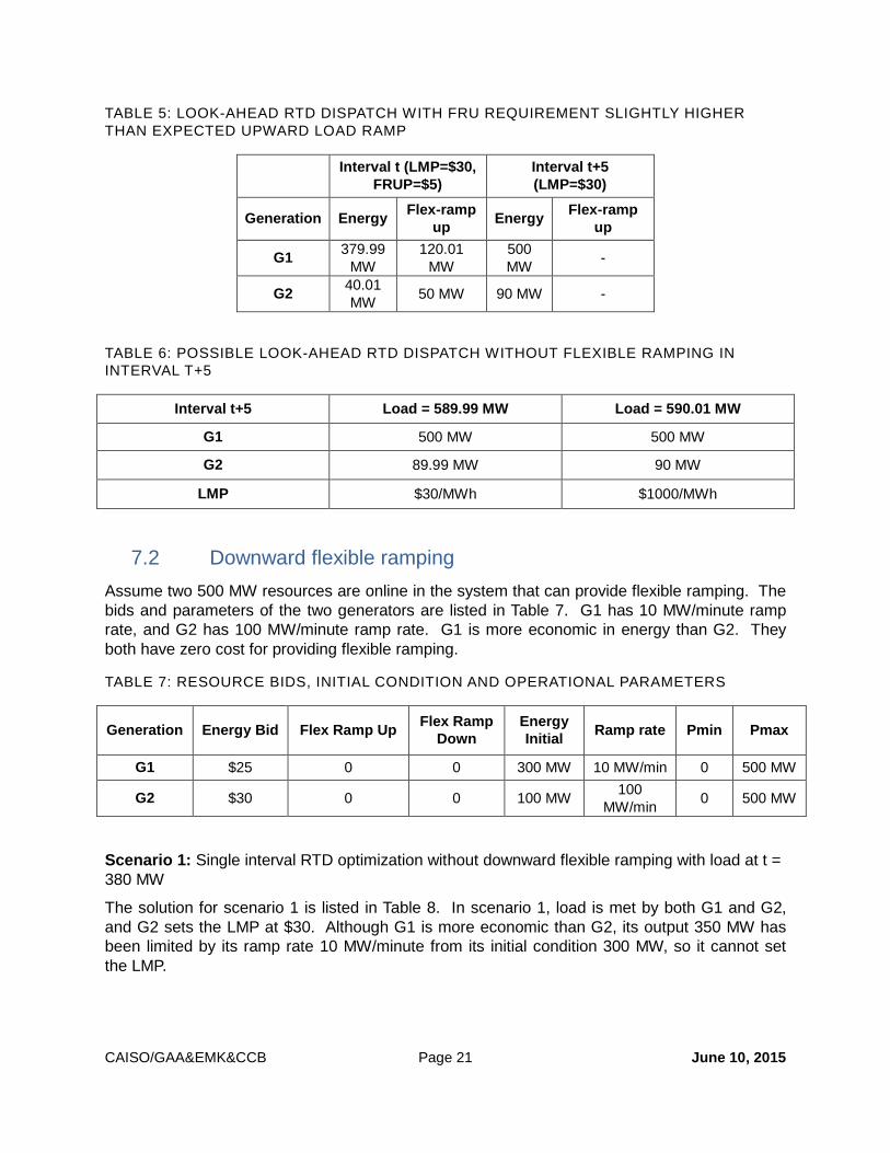
In scenario 4, both flexible ramping and look-ahead are modeled in the optimization. In order to have uniquely determined prices, we set upward flexible ramping requirement slightly higher than expected load ramp 170 MW. The results are listed in Table 5 which converge to scenario 2 in the first interval. If the flexible ramping requirement is slightly lower than the expected load ramp, the solution would converge to scenario 3.


TABLE 5: LOOK-AHEAD RTD DISPATCH WITH FRU REQUIREMENT SLIGHTLY HIGHER THAN EXPECTED UPWARD LOAD RAMP

Interval t (LMP=$30, FRUP=$5)

Interval t+5 (LMP=$30)

Generation Energy Flex-ramp up Energy Flex-ramp

up

G1 379.99 MW

120.01 MW

500 MW -

G2 40.01 MW 50 MW 90 MW -

TABLE 6: POSSIBLE LOOK-AHEAD RTD DISPATCH WITHOUT FLEXIBLE RAMPING IN INTERVAL T+5

Interval t+5 Load = 589.99 MW Load = 590.01 MW

G1 500 MW 500 MW

G2 89.99 MW 90 MW

LMP $30/MWh $1000/MWh

7.2 Downward flexible ramping Assume two 500 MW resources are online in the system that can provide flexible ramping. The bids and parameters of the two generators are listed in Table 7. G1 has 10 MW/minute ramp rate, and G2 has 100 MW/minute ramp rate. G1 is more economic in energy than G2. They both have zero cost for providing flexible ramping.

TABLE 7: RESOURCE BIDS, INITIAL CONDITION AND OPERATIONAL PARAMETERS

Generation Energy Bid Flex Ramp Up Flex Ramp Down

Energy Initial Ramp rate Pmin Pmax

G1 $25 0 0 300 MW 10 MW/min 0 500 MW

G2 $30 0 0 100 MW 100 MW/min 0 500 MW

Scenario 1: Single interval RTD optimization without downward flexible ramping with load at t = 380 MW

The solution for scenario 1 is listed in Table 8. In scenario 1, load is met by both G1 and G2, and G2 sets the LMP at $30. Although G1 is more economic than G2, its output 350 MW has been limited by its ramp rate 10 MW/minute from its initial condition 300 MW, so it cannot set the LMP.


TABLE 8: SINGLE-INTERVAL RTD DISPATCH WITHOUT DOWNWARD FLEXIBLE RAMPING


Generation Energy Flex-ramp down

G1 350 MW - G2 30 MW -

Scenario 2: Single interval RTD optimization with downward flexible ramping with load at t = 380 MW and downward flexible ramping requirement at t = 170 MW

The solution for scenario 2 is listed in Table 9. In scenario 2, in order to meet 170 MW downward flexible ramping, G2 needs to be dispatched up in order to provide downward flexible ramping. As a result, G1’s output will be reduced in order to maintain the power balance, and G1 sets the LMP at $25. Note the downward flexible ramping requirement causes the LMP to decrease compared with scenario 1. The downward flexible ramping price FRDP is set by G2’s energy price deficit $30 – $25= $5. The FRDP price is to compensate G2 such that G2’s revenue including both energy and FRD can cover its energy bid cost $30. As a result, there is no revenue shortage for G2, and no need for bid cost recovery.

TABLE 9: SINGLE-INTERVAL RTD DISPATCH WITH DOWNWARD FLEXIBLE RAMPING

Interval t (LMP=$25, FRDP=$5)

Generation Energy Flex-ramp down

G1 260 MW 50 MW

G2 120 MW 120 MW

Scenario 3: Two-interval RTD optimization without downward flexible ramping with load at t = 380 MW and load at t+5 = 210 MW.

The solution for scenario 3 is listed in Table 10. In scenario 3, there is no FRD requirement. However, the look-ahead optimization projects a 170 MW of downward load ramp from interval t to t+5, which equals the downward flexible ramping requirement in scenario 2. The look-ahead optimization produces the same dispatch for interval t as in scenario 2, but different LMPs. The dispatch is the same because the look-ahead load ramp also requires the same amount of ramping capability as the flexible ramping requirement in interval t. The LMPs are different because there is an interaction between the energy price and flexible ramping price. When net system demand is increasing, which creates more downward ramp need, the look-ahead optimization will increase the energy price in the binding interval (for similar but opposite reasons as described in the FRU example in scenario 3 in the preceding section (7.1).


TABLE 10: LOOK-AHEAD RTD DISPATCH WITHOUT DOWNWARD FLEXIBLE RAMPING


Interval t+5 (LMP=$20)

Generation Energy Flex-ramp down Energy Flex-ramp down

G1 260 MW - 210 MW -

G2 120 MW - 0 -

8. Settlement The ISO will financially settle FRP in the fifteen-minute market and the five-minute market. To reduce implementation complexity, the ISO proposes to drop its previous proposal for “no-pay” rules that were virtually the same as the existing ancillary services no-pay and instead implement real-time economic buy-back rules that will be somewhat similar to uninstructed imbalance energy (UIE) settlement.

The proposed real time economic buy-back rules will prevent resources from receiving an FRP payment if they cannot provide what the real-time market awarded. A resource would pay back unavailable FRP capacity at the RTD FRP price. The ISO is still evaluating how it would measure unavailable FRP capacity. The alternatives are:

• Compare a resource’s metered output, upper and lower economic limits to the FRP award to determine if the resource could provide its awarded FRP (similar to the “undispatchable” and “unavailable” no-pay provisions). Depending on implementation complexity, this alternative could consider the resource’s actual ramping capability, or imply compare the FRU or FRD award to the difference between the metered output and the resource’s upper and lower economic limits, respectively.

• Simply assume any positive UIE makes the corresponding amount of FRU unavailable and any negative UIE makes the corresponding amount of FRD unavailable.

The ISO seeks stakeholder input on these alternatives.

The example shown in Table 11 and Table 12 shows an example of the energy and FRP settlement for a resource that is scheduled for energy and awarded FRU for a time period representing one FMM interval and the corresponding RTD intervals, 7:00 – 7:15.

Table 11 illustrates the real-time market energy settlement for this resource. The top portion, under “Schedule MW,” shows the resource’s market schedules, meter values, as well as instructed imbalance energy (IIE) and UIE quantities. Under “Price ($/MWh), it shows the corresponding energy prices. The bottom portion, labeled “Settlement ($)” shows the calculation and results of the settlement of these imbalance energy quantities (UIE settlement is listed under “Meter”).

In this example, the resource does not have a day-ahead schedule so the full amount of the FMM schedule is settled as FMM IIE. The difference between the RTD dispatch and the FMM


schedule is settled as RTD IIE. The difference between the meter and the RTD dispatch is settled as UIE.

TABLE 11: AN ENERGY SETTLEMENT EXAMPLE

SCHEDULE (MW) PRICE ($/MWH)

TIME 7:00 7:05 7:10 7:00 7:05 7:10

FMM 402 402 402 $30 $30 $30

RTD 302 415 402 $25 $36 $25

METER 420 420 430 $25 $36 $36

FMM IIE (MWH)

33.5 33.5 33.5 $30 $30 $30

RTD IIE (MWH)

-8.33 1.08 0.00 $25 $36 $25

UIE (MWH) 9.83 0.42 2.33 $25 $36 $25

SETTLEMENT ($)

TIME 7:00 7:05 7:10 7:00 7:05 7:10

FMM FMM/12 * FMM PRICE

FMM/12 * FMM PRICE

FMM/12 * FMM PRICE

$1,005 $1,005 $1,005

RTD (RTD IIE)* RTD PRICE

(IIE)* RTD PRICE

(IIE)* RTD PRICE

-$208.33 $39.00 $0.00

METER (UIE) * RTD PRICE

(UIE) * RTD PRICE

(UIE) * RTD PRICE

$245.83 $15.00 $58.33

TOTAL SUM COLUMN

SUM COLUMN

SUM COLUMN

$1,043 $1,059 $1,063


Table 12 is set-up similar to Table 11 but illustrates FRP settlement, showing the FRU settlement for this hypothetical resource.

It shows FRP is settled somewhat similar to imbalance energy, the difference being the settlement for the unavailable FRP (illustrated as “unavailable FRU” in Table 12). Unavailable FRP is roughly analogous to UIE in that it represents the settlement for a quantity that is due to a deviation from the ISO’s dispatch instruction. Unavailable FRP differs from UIE settlement in that the ISO would only settle unavailable FRP so that the resource buys-back FRP that was scheduled or dispatched by FMM or RTD but not available, while UIE can be settlement for energy in addition to that scheduled or dispatched by FMM or RTD

In this example, the unavailable FRU is determined by calculating the available ramping by comparing the resource’s meter to its upper economic limit. In RTD interval 7:10, RTD dispatched the resource for 20 MW of FRU, but because the resource’s meter equates to 430 MW, a deviation from its 402 MW RTD dispatch, it only has 5 MW of remaining capacity. Consequently, 15 MW of its 20 MW RTD FRU dispatch is settled as unavailable FRU at the RTD FRU price. (The unavailable FRU would be the same for any of the alternatives to determine unavailable FRU outlined at the beginning of this section.)


TABLE 12: FRU SETTLEMENT EXAMPLE

Schedule (MW) Price ($/MWh)

Time 7:00 7:05 7:10 7:00 7:05 7:10

FMM 15 15 15 $6.00 $6.00 $6.00

RTD 6 15 20 $5.00 $10.00 $12.00

RTD Delta (MW)

-9 0 5 $5.00 $10.00 $12.00

Upper economic limit

435 435 435

Meter 420 420 430

Available ramping

15 15 5

Unavailable FRU (MW)

0 0 -15 $5.00 $10.00 $12.00

Settlement ($)

Time 7:00 7:05 7:10 7:00 7:05 7:10

FMM FRU FMM/12 * FRU FMM price

FRU FMM/12 * FRU FMM price

FRU FMM/12 * FRU FMM price

$7.50 $7.50 $7.50

RTD RTD Delta FRU / 12* FRU RTD price

RTD Delta FRU / 12* FRU RTD price

RTD Delta FRU / 12* FRU RTD price

-$3.75 $0.00 $5.00

Meter Unavailable FRU /12 * FRU RTD price

Unavailable FRU /12 * FRU RTD price

Unavailable FRU /12 * FRU RTD price

$0.00 $0.00 -$15.00

Total Sum column

Sum column

Sum column $3.75 $7.50 -$2.50


9. Cost allocation

9.1 Proposed movement baseline The ISO will allocate the costs for the flexible ramping product based upon supply and demand “movement” that requires the ISO market to dispatch other resources in the five-minute real-time dispatch.

• Load movement is defined as five-minute changes in forecasted ISO load.

• Intertie movement (fixed ramps) is calculated based upon the netted change in MWhs deemed delivered every five minutes for all imports/exports plus operational adjustments not reflected in the FMM schedule.

• Supply movement (besides interties) is defined as five-minute netted supply imbalance changes that are not the result of an ISO economic five-minute dispatch instruction. This can either be certain dispatched movement (e.g. self-schedule changes, non-economically bidding variable energy resource forecast changes) or uninstructed deviations from ISO dispatch instructions.

The ISO market will procure upward flexible ramping product to address negative movement between dispatch intervals. The ISO market will procure downward flexible ramping product to address positive movement between dispatch intervals.

The following examples show the calculation of movement for each category in interval “RTD 1.” The supply category requires the RTD dispatch to be differentiated between those dispatches that are in response to imbalance needs and those dispatches that create imbalance needs. Table 13 provides an example where load increases 10 MW between the first interval “RTD 1,” and the second interval, “RTD 2.” Because load increases 10 MW, it is allocated 10 MW of FRU. In this example, the intertie moves from 100 MW to 105 MW. This would typically occur such as at the end of the hour when the intertie is ramping up to a different hourly schedule. The five-minute real-time dispatch must dispatch other resources down to account for this movement. Therefore, the intertie is allocated 5 MW of FRD. Finally, this example shows supply being economically dispatched to balance the load and intertie movement. Therefore, supply is not allocated either FRU or FRD.


TABLE 13: PROPOSED MOVEMENT BASELINE

Movement RTD 1 RTD 2 FRU movement

FRD movement

Load: load forecast 1,000 MW 1,010 MW 10 MW 0 MW

Intertie: deemed delivered 100 MW (import)

105 MW (import)

0 MW 5 MW

Supply: multiple resources - economic bids dispatched within bid range

900 MW 905 MW 0 MW 0 MW

Table 14 provides an example where load decreases between the first interval “RTD 1,” and the second interval, “RTD 2.” from 1,100 MW to 1,080 MW and is therefore allocated 20 MW of FRD. The intertie increases its export from 200 MW to 210 MW and the five-minute real-time dispatch must dispatch other resources up to meet the imbalance. Therefore the intertie is allocated 10 MW of FRU.

Table 15 also provides examples of the allocation to several supply resources. Resource A can be thought of as a variable energy resource that is economically bidding, whose forecast to which the five-minute real-time dispatch is dispatching has declined. This resource’s movement requires another resource to be dispatched up 15 MW in RTD 2 to balance the decreased output. If this resource’s forecast had actually increased in RTD 2, it would not be allocated FRD assuming it was economic to dispatch this resource at its forecast. The allocation of FRD to decreased forecast output is the same treatment as a conventional resource which has a de-rate of its PMax between RTD intervals.

Resource B illustrates the similar treatment for changes in the PMin of resources participating economically. A re-rate of a resource’s PMin would require the other resources to be dispatched down to offset the resources increased output.

Resources C and D illustrate resources that are not participating economically but have movement because of changes to their upper or lower economic limit because of changes to Pmax or PMin. In these cases, other resources must be dispatched to meet the changes in output of the resource. If Resource D’s dispatch was caused by a manual dispatch it would receive no allocation because it would otherwise not be dispatched down. Resource D would also receive no allocation if its dispatch was caused because an otherwise flat self-schedule that was reduced via penalty parameters to address a transmission constraint.

The remaining resources provide economic bids and are dispatched within their bid range. Therefore the remaining supply is not allocated any FRU or FRD movement.


TABLE 14: PROPOSED MOVEMENT BASELINE

Movement RTD 1 RTD 2 FRU FRD

Load: load forecast 1,100 MW 1,080 MW 0 MW 20 MW

Intertie: Demand delivered 200 MW (export)

210 MW (export)

10 MW 0 MW

Supply: Res A- No economic bids and dispatch at upper economic limit

150 MW 135 MW 15 MW 0 MW

Supply: Res B- Economic bids and dispatch at lower economic limit

100 MW 110 MW 0 MW 10 MW

Supply: Res C- No economic bids and dispatch at upper economic limit

150 MW 160 MW 0 MW 10 MW

Supply: Res D- No economic bids and dispatch at lower economic limit

100 MW 95 MW 5 MW 0 MW

Supply: multiple resources - economic bids dispatched within bid range

800 MW 790 MW 0 MW 0 MW

9.2 Billing determinant of load category The ISO will use gross uninstructed imbalance energy to determine the share of flexible ramping costs attributable to load. The allocation will be based upon five-minute net uninstructed imbalance energy. It should be noted that in addition to the flexible ramping product allocation, load following MSS are subject to penalties for excessive deviations.

If a load uses five minute metering, such as load following metered sub-systems, then the load would be considered within the supply category.

9.3 Billing determinant of supply category The supply category will be allocated based upon the five minute-resource specific movement. In determining the shares of FRU and FRD to be allocated to the supply category, uninstructed deviations will net against other five-minute movement that otherwise would receive a FRU or FRD allocation.

Conventional supply resources and variable energy resources will have their five-minute resource specific movement. Conventional resources that economically bid into the real-time market will not have any five-minute movement unless the resource has a re-rate of Pmin or Pmax. If a variable energy resource economically bids in the real-time market, the only FRP allocation it will receive will be for FRU. It will be allocated FRU in intervals where its forecast output declines.


9.3.1 Threshold for allocation The ISO will apply a minimum threshold in allocating movement within the supply category. The threshold is as follows:

𝑇ℎ𝑟𝑟𝑟ℎ𝑜𝑜𝑑 = min (𝐸𝐸𝑟𝑟𝐸𝐸 𝑆𝑆ℎ𝑟𝑑𝑒𝑜𝑟 (𝑀𝑀) ∗ .03, 5𝑀𝑀)

A resource will not be allocated FRU or FRD costs for movement less than the threshold. For example, assume a resource has instructed energy of 10 MW in a given settlement interval, if the resource’s five minute movement and is less than 0.3 MW the resource’s would not be allocated FRU or FRD costs. If the five-minute movement and uninstructed is greater than 0.3 MW, the resource would be allocated FRU and FRD costs. A minimum threshold will also apply. The minimum threshold will be the minimum of 3% instruction or 5 MW.

9.4 Billing determinant of intertie fixed ramp category The ISO will not allocate FRP costs to 15-minute schedule changes of imports/exports economically participating in the FMM. The 15-minute schedule changes do have prescribed 10-minute ramps: however, the subsequent FMM run can modify the five-minute ramp at the end of the fifteen-minute interval) to be consistent with changing system conditions in FMM.

In contrast, the ISO market must honor modeled ramps for hourly schedules even if the ramp is counter to existing system conditions. As such, these fixed ramps for hourly intertie schedule changes will be allocated FRU and FRD costs.

However, when the fixed ramp movement is aligned with the load change, the allocation will be for the FRP in the opposite direction of load movement. This should limit the costs allocated since there should be more FRP supply relative to demand in the opposite direction of load movement. For example, in the morning load pull, the ISO will require more FRU. If in this hour, net imports are increasing, intertie’s fixed ramp movement will be positive which results in an allocation of FRD rather than FRU.

9.5 Monthly re-settlement Since the flexible ramping products are procured based upon forecasted movement, when a resource deviates in a specific settlement interval, it is not correct to conclude that the resource’s actual deviation caused the flexible ramping product to be procured for that settlement interval. Consistent with the “synchronization” cost allocation guiding principle,2 the ISO proposes to re-settle costs based upon the monthly rate per deviation for each operating

2 http://www.caiso.com/informed/Pages/StakeholderProcesses/CompletedStakeholderProcesses/CostAllocationGuidingPrinciples.aspx


hour. The monthly rate will be determined by the total costs incurred during the month divided by the sum of positive (or negative for FRU) deviations across all resources within a category for each operating hour. On an hourly basis, scheduling coordinators will be allocated flexible ramping product costs as a share of their deviations. At the end of the month, these hourly charges will be reversed, and the scheduling coordinator will be charged the monthly rate for each of its five minute deviations for each hour of the day.

The monthly re-settlement process is done separately for both the FRU and FRD products. The overall FRU and FRD settlement process, including daily settlement and the monthly resettlement, is as follows:

Step 1 Determine hourly balancing authority area cost for the product. The total cost of all constraints across all markets.

Step 2 Determine the 5-minute gross movement for each category in the hour within the balancing authority area.

Step 3 Calculate costs of each category using its share of 5-minute movement for the relevant product.

Step 4 Allocate the hourly costs within the category according to the rules of that category using 5-minute data from that hour.

Step 5 At the end of the month, reverse all hourly settlements within the balancing authority area.

Step 6 Sum product costs for each hour over the month.

Step 7 Sum the 5-minute gross movement for each category for each hour over the month.

Step 8 Calculate the monthly cost for each hour by using the category’s share of the monthly 5-minute movement of the relevant product.

Step 9 Allocate the monthly costs within the category according to the rules of the category using 5-minute data summed for that hour over the month.

Draft Technical Appendix - caiso.com

Documents

Transcript of Draft Technical Appendix - caiso.com