draft opaqueness income shocks - EFMA ANNUAL MEETINGS/2016-… · income shocks Frederiek Schoubben...

1

The role of an insurer’s opaqueness on the reaction to

income shocks

Frederiek Schoubben, Cynthia Van Hulle*1

(preliminary draft, do not quote without permission)

January, 2016

Abstract

The insurance literature shows that there are many characteristics that influence the ability to

accurately evaluate the financial strength of an insurer going from risk taking over capitalisation

to organisational form. This study is the first to investigate whether these determinants of

insurer opaqueness also influence the efficiency change following an important income shock.

As an insurer can always rely on internal funds to gradually rebuild equity following negative

income events, it is not a priori clear for outsiders like policy holders whether a particular shock

will influence future financial health. Especially the more opaque insurers are pressured to

restore performance more rapidly as they want to avoid that income shocks are perceived as

signals of bad financial soundness causing loss of reputation and customer business. Our

empirical results based on stochastic frontier analysis on a set of European insurers support the

hypothesis that although an income shock always triggers a positive efficiency change in the

following years, insurers that are characterised as more opaque will increase efficiency beyond

simply absorbing the income shock with the solvency buffer.

*Frederiek Schoubben (corresponding author): KU Leuven, Faculty of Economics and Business, Department of

Financial Management, Korte Nieuwstraat 33, 2000 Antwerp, Belgium; email:

[email protected]

Cynthia Van Hulle: KU Leuven, Faculty of Economics and Business, Department of Accountancy, Finance and

Insurance, Naamsestraat 69, 3000 Leuven, Belgium; email: [email protected]

2

Introduction

In corporate finance, a number of studies document the behavior of, and the triggers of change

in, non-financial firms that have met with an important performance decline (e.g., John et al.,

1992; Kang and Shivdasani, 1997; Denis and Kruse, 2000). It has been shown in this literature

that companies can counter poor performance in a variety of ways, from operational changes

over cost or revenue efficiency actions to governance related disciplining of management.

Furthermore, the capacity to engage in successful turnaround strategies proves to depend on the

disciplinary environment of the financial/product markets or the internal governance

mechanisms. All studies show that these action are primarily aimed at cash conservation within

the firm and improvement of efficiency to enhance future cash generation capacity.

For insurance companies, unlike non-financial firms, upfront financing of vast amounts of fixed

assets and working capital are not an issue. Insurers have an inverted production cycle, i.e. they

receive upfront payment from policy holders and only afterwards have to pay out claims.

Furthermore, they need relatively little fixed assets and working capital (i.e. illiquid assets) to

operate but are obliged by law to invest the (fair) value of future claims in mostly tradeable

securities (Dhaene et al., 2015). An important question is therefore whether due to this inverted

cash cycle, insurance companies are truly triggered to react on income declines and are not just

waiting until the situation is restored. This view is certainly in line with the business cycle view

on insurers where insures rely on internal funds to gradually rebuild equity (Weiss, 2007). This

would suggest that no immediate action is taken other than using the solvency buffer in order

to absorb the income shock. However, one important reason why (not all) insurers can’t fully

exploit the flexibility offered by business cycles and would still feel pressured to actively react

upon a setback, is rooted in their relation with their customers (i.e., policy holders). Contrary to

a typical non-financial company, the customers of an insurer become the firm’s debt holders

through their future claims. As a result, an important set back may harm the insurers’ reputation

and soundness, causing customers to walk away (e.g., Eppermans and Harrington, 2006). This

problem is even intensified when an accurate evaluation of default probabilities is more difficult

due to risk taking, capitalization or organizational form (Pottier and Sommer, 2006). More

opaque insurers will want to make sure that the income shock is not perceived as a signal of

bad financial soundness which pressures them to restore performance more rapidly by

increasing efficiency.

This study analyses whether common determinants of insurer opaqueness influence the

efficiency change following an important income shock measured as a strong relative decline

3

in return on assets. As insurance firms generally rely heavily on retained earnings as their main

source of capital (Shim, 2010), profitability shocks will generate attention by the stakeholders

as well as the management of an insurance company. By using stochastic frontier analysis on a

set of 1454 non life insurers in 19 European countries over the period 2003-2013, we find that

insurers confronted with an important profitability shock increase productivity with 3% to 5%

in the following years. A big portion of that increase however is represented by the temporary

reduction in solvency indicating the above mentioned exploitation of flexibility offered by the

insurers’ business model. When the decrease of the solvency buffer is taken into account, an

interesting picture emerges. Only the insurers with high levels of our proxies for opaqueness

(e.g., reinsurance, income and product uncertainty, long tail business,…) increase productivity

significantly compared to matched non shock firms. This strongly indicates that these more

opaque insurers are pressured to restore performance more rapidly by increasing efficiency

beyond the solvency change. Our results therefore prove that the determinants of insurer

opaqueness strongly influence the reaction to an income shock.

Our study contributes to the literature in several ways. First, to our knowledge there is no study

exploring the efficiency effects of performance declines in particular. Few studies address

efficiency changes following particular events like CEO turnovers (He et al., 2011), merger and

acquisitions (Cummins and Xie, 2008) and demutualization (Chen et al., 2011). Second, the use

of efficiency measures contributes to earlier studies that use financial ratio’s, as efficiency

scores are able to capture firm performance in a single measure that controls for differences

among insurers in a multidimensional framework. Third, we contribute to the insurance

literature as well as the corporate finance literature by studying whether the insight from studies

on restructuring still apply to a business model where efficiency increase is not primarily aimed

at the enhancement of future cash generation. Finaly, our study is also relevant from a policy

perspective as the insurance industry plays a vital role in the global economy both in reducing

uncertainties as in providing long term financial resources. In 2013, premiums written

worldwide amounted to approximately 4.6 trillion US dollars while investments in financial

assets represented about 37% of worldwide GDP (Swiss Re, 2014). European insurers even

surpass their US counterparts in terms of worldwide market share with 35% over 30%

(Insurance Europe, 2014). Moreover, as the existing European regulatory framework is in

transition towards the unified regulatory framework of Solvency II, an enhanced understanding

of the link between profitability, solvency and productivity could generate important policy

implication.

4

The article is organized as follows. First, we give an overview of the insurance literature on

firm behaviour following important events as well as studies on both efficiency measurement

and opaqueness in the insurance industry. We then develop the hypotheses concerning the

efficiency change in the years following an important income shock. Next, we discuss the data,

variable definitions and the method employed to analyse the insurers’ reactions to income

shocks depending on opaqueness. Finally we present our empirical evidence and discuss the

results.

2Literature review

Insurer behaviour following performance decline

Several papers study specific aspects of behavior of insurers following a strong change in

performance. In particular, the impact of downgrades on market reaction and premium change

has been extensively studied in the insurance literature. Rating downgrades have been shown

to trigger declines in insurance premiums (Epermanis and Harrington, 2006) as well as

insurance demand (Baranoff and Sager, 2007). Similarly, rating downgrades are usually

accompanied by a negative stock market reaction (Halek and Eckles, 2010). Wang and Carson

(2014) find that rating changes are positively correlated with future rating changes but that this

effect is strongly influenced by the initial rating, where insurers with higher initial ratings suffer

less from a downward spiral of consecutive downgrades.

Besides rating changes, also the impact of income shocks due to catastrophic events on

insurance companies has been studied. Although the overall effect of catastrophes depends on

the nature of the event, most studies show that insurance companies are usually resilient enough

to recuperate from severe catastrophe related income shocks. Insurers tend to recoup

catastrophe losses through adjustments to premiums. However, the recovery of individual

insurance companies strongly depends on the competition within the relevant insurance market

(Hagendorff et al., 2015), the initial financial strength of the insurer (Cummins and Lewis,

2003) as well as the pre-loss leverage (Doherty et al., 2003).

In the same vein, the insurance literature documents the existence of so called underwriting

cycles (e.g. Weis, 2007). Basically, this literature takes the perspective that it is costly for

insurers to issue equity after a loss or negative investment shock due to asymmetric information

and other market imperfections. In turn, because of interactions between financing and business

plans, this temporary lack of equity - that first needs to be rebuild through internal funds - results

5

in higher prices and/or less insurance supply. Although theories about underwriting cycles are

established at the industry level, there is ample empirical evidence of its influence on insurers

at the firm level (e.g. Doherty and Posey, 1997; Cummins and Danzon, 1997; Doherty and

Phillips, 2002; Weiss, 2007; among others). In fact, Weiss (2007) claims that the policy holder’s

demand for safe insurance causes cross sectional differences among insurers depending on the

perceived default probability.

Efficiency measurement in the insurance industry

Measuring the efficiency of the operations of an insurer and the (governance) forces that cause

cross sectional differences in firm efficiency, has also received much research attention in the

insurance literature. Most studies (see Cummins and Weiss, 2013 for an extensive literature

review) consider one (or all) of the following aspects: geographical (i.e., country)

characteristics, regulatory differences, organizational (governance) forms and lines of business.

Although the results tend to differ considerably depending on the sample period and the

methodology used, most studies find an impact of these characteristics on efficiency scores.

Interestingly, considering the vast amount of research on cross sectional differences in

efficiency scores, very few studies address efficiency changes following particular events like

CEO turnovers (He et al., 2011), merger and acquisitions (Cummins and Xie, 2008) and

demutualization (Chen et al., 2011). Moreover, to our knowledge there is no study exploring

the efficiency effects of performance declines in particular.

Cross country studies on European insurance industry (Fenn et al. 2008) generally find

increasing productivity over the last decades due to deregulation and consolidation in the

financial services markets in general. Eling and Luhnen (2010) provide an efficiency

comparison of insurers from 36 countries and report a steady efficiency growth in international

insurance markets from 2002 to 2006. Bertoni and Croce (2011) investigate the drivers of

productivity in the life insurance industries of five European countries (Germany, France, Italy,

Spain, and the United Kingdom). They find increased productivity is mostly due to innovation

in best practices, which is attributable to technological change.

Efficiency changes following particular events has not benefited from much research attention.

The studies that do measure firm performance using efficiency changes generally test whether

the event triggered a particular difference in efficiency measures between the pre and post event

period, and whether firm characteristics affected this change. He et al. (2011) for example show

6

on a set of US non-life insurers that CEO turnovers (especially the non-routine ones) triggered

a performance increase in the years following the event. They conclude that when there is a

forced replacement of a poor managers with a better one, overall efficiency improves. Chen et

al. (2011) show that also a change in organizational form might influence efficiency. They show

that U.S. property-liability insurers improve their efficiency performance when converting from

mutual to stock ownership.

Insurer opaqueness

Opaqueness is inherent to the financial services industry. For outside stakeholders like

customers or regulators, opacity results from information uncertainty that can arise from

incomplete disclosure, disclosure quality or simply the disclosure complexity. Information

about the underlying profitability and risks of the firm or the ability of managers to rapidly

transform assets can therefore be difficult to assess. Easley et al. (2002) and Easley and O’Hara

(2004) show that information risk affects asset returns and the cost of capital. Asset composition

is widely acknowledged in the banking literature as an important determinant of opacity.

Morgan (2002) shows that banks are relatively more opaque than non-banks. Examining dual-

rated debt issued by banks and non-banks over the period 1983–1993, he finds that bank debt

is more likely to be split rated than non-bank debt. More importantly, loans and trading assets,

which increase the likelihood that newly issued bank debt will be split rated, represent

significant sources of opacity for banks.

Within the financial services industry, insurers are considered even more opaque than banks.

The reason for this is that in contrast to banks, insurers encounter information asymmetry in

both assets and liabilities. Morgan (2002) shows that there is more disagreements among rating

agencies concerning the financial health of insurers compared to banks. This opacity among

insurers is not surprising. The insurer underwrites insurance policies whose actuarial loss

estimation is both uncertain and unknown to outsiders. Moreover, a big part of an insurers’

liabilities comprises of a loss reserve which is a prediction of future claim payments. Disclosing

details on the methodology used to value future risks however might be detrimental for the

firm’s competitive position. Therefore, a level of opacity can never be discarded when it comes

to insurers. The permitted, even desirable, information asymmetry between insiders and

outsiders provides manages with considerable discretion about the risk valuation methods and

corresponding technical reserves (Petroni, 1992). Babbel and Merrill (2005) argue that the

inherent complexity and opaqueness of insurance contracts even provides insurance managers

7

with opportunities to manage the disclosed value of loss reserves and surplus. This enables

insurance managers to take advantage of their less-informed customers.

Besides the stochastic nature of the liabilities, also the asset side of tha balance sheet might be

a source of insurer opacity. A large portion of these assets is relatively liquid due to the need to

quickly convert assets to cash in order to meet business demands. Myers and Rajan (1998) claim

that while liquid assets should be highly transparent, the ability to convert such assets to

completely different positions quickly and efficiently brings about another source of potential

opacity for insurers. Zhang et al. (2009) find that insurers underwriting more opaque lines of

business are subject to higher adverse selection costs.

In the insurance literature, opaqueness is usually measured by looking at rating disagreement

among agencies. Several papers try to determine the source of opaqueness by analysing the

impact of insurer characteristics on such disagreement among rating agencies. Pottier and

Sommer (2006) for example find for a cross section of property and casualty insurers that

financial health rating disagreement, and thus opaqueness, depends on insurer characteristics

like size, organisational form, reinsurance use and geographical diversification. Adamson et al.

(2014) extend the work of Pottier and Sommer (2006) by using panel data of both life and non

life insurance companies and use disagreement in bond ratings as a measure of opaqueness.

They find higher levels of opaqueness among mutual insurers. Finally, Zang et al. (2009)

explore the effects of asset and liability opacity from the perspective of the secondary stock

market using bid-ask spreads, controlling for financial factors, the activity of informed traders,

and other trading characteristics. Their results indicate that insurers underwriting more opaque

lines of business are subject to higher adverse selection costs. On the other hand more analyst

coverage seems to reduce information asymmetry and, therefore, insurer opaqueness.

Hypothesis development

A sizeable literature shows that the pressure from different stakeholders/governance

mechanisms shape choices made by insurers (see Boubakri, 2011 and 2013, for an overview of

the literature). Important stakeholders in the context of the insurance industry include

policyholders, insurance agents, regulators and rating agencies, reinsurers and outside board

members (Cole et al., 2011). Recent literature (a.o., Cheng et al., 2015; Eling and Marek, 2014)

shows that these stakeholders play a distinctive role in controlling agency conflicts and

8

monitoring solvency risk depending on the organizational structure (e.g., mutual versus stock

insurance companies), ownership structure (e.g., institutional ownership, insider ownership)

and governance characteristics (e.g., board composition, executive compensation, CEO

duality).

When looking at an income shock in a certain year it is not a priori clear whether and why this

would influence firm performance in the form of efficiency changes in the following years. As

already mentioned in the introduction, insurers are able to use their inverted business cycle in

order to restore performance gradually without increasing actual productivity. The relationship

between an insurer and its policy holders might be of vital importance in understanding firm

behavior following shock events. Policy holders can even be seen as a source of discipline (e.g.,

Epermanis and Harrington, 2006; Baranof and Sager, 2007). Epermanis and Harrington (2006)

show that in a context of downgrades, that insurers tend to lower premiums in order to avoid

losing insurer business. Baranoff and Sager (2007) even find evidence for a decline in insurance

demand in the years following a downgrade. The authors claim that this market discipline

through consumer pressure should be considered as an additional protection against insolvency

besides the external regulatory/rating and internal governance mechanisms. A similar flight to

quality risk is also observed in the context of catastrophe events (Hagendorff et al., 2015).

Policyholders are sensitive to the insolvency risk of their insurance company, especially when

the policyholders are insufficiently protected by the asset portfolio or by a guarantee fund (De

Haan and Kakes, 2010). The income drop might therefore trigger a flight to quality similar to

the behavior documented in the literature on catastrophe events or downgrades. Based on these

arguments we propose the following hypothesis

H1 In order to reduce the threat of losing customer business, insurers react to an income

shock by increasing efficiency.

The actual threat of losing business will strongly depend on the demand elasticity of customers.

It is paramount for good insurers not to be confused with poor performers. Papers studying the

recovery after catastrophes or downgrades already showed that the initial financial strength

plays an important role in the ability of the insurer to recuperate. However, these papers never

question the fact that the financial strength is not equally assessable among insurers. The

opaqueness literature shows that there might be strong disagreement among rating agencies

depending on several characteristics (Pottier and Sommer, 2006). It would even be harder for

9

customers to evaluate the impact of an income shock to overall future financial health. This

would pressure the most opaque insurers to react more rapidly to avoid additional scrutiny by

outsiders in general and costumers in particular. Therefore, opaqueness will limit the flexibility

of insurers to use their business cycle in order to gradually restore performance. This leads to

our second hypothesis.

H2 The impact of an income shock on efficiency will be more pronounced in more

opaque insurers

Data, Sample and methodology

Data and sample selection

We use Bureau van Dijk’s ISIS database to obtain accounting information for initially 1893

European non-life insurers from 2003 to 2013. As this is a cross country data base we also

require a minimum of 10 firm year observations per country to be able to control for the country

fixed effects in the multivariate models. This leads to a final set of maximum 1454 insurers

corresponding to 11489 firm year observations. However, due to the extensive use of lagged

values both in the SFA methodology as in the measurement of certain variables, the effective

sample in the reported univariate and multivariate results is always somewhat smaller. Insurers

are not required to have data for all years but since efficiency changes over at least 3 up to 5

consecutive years are estimated, several insurers that fail this minimum requirement are not

included in the respective estimation models. Additionally, as in Eling and Luhnen (2010), we

only include insurers with positive values for inputs as well as outputs in order to get

meaningfull efficiency scores. Table 1 provides an overview of the maximum number of firm

year observations over the countries (Panel A) and years (Panel B) in our sample. Notice that

our sample comprises of eastern as well as western European countries.

Opaqueness measures

The insurance literature puts forward several firm characteristics that can be associated with

opaqueness. We will use these measures to study whether the difficulty to assess financial

strength forces them to react more strongly to income shocks.

10

A first measure of opaqueness is the intensity with which reinsurance is used by the insurer.

Insurers that rely heavily on reinsurance will be more opaque as their financial soundness no

longer depends solely on their own characteristics but also the financial strength of the reinsurer

firm. Analogue to Sommer and Pottier (2006), we measure reinsurance usage as the difference

between gross claims and net claims divided by premiums written. Insurers with an above

median level of this ratio get the value 1 on the opaqueness dummy.

Another important source of opaqueness is the uncertainty surrounding the insurer’s operations.

Although an insurer is in the business of risk, there are still concerns about the way this risk is

hedged. In other words, if the risk is correctly handled there should be less uncertainty. An

insurer with very high variability of income is obviously harder to evaluate compared to an

insurer with a steady income stream. In line with Eling and Marek (2013), we define two distinct

opaqueness measures depending on the source of the uncertainty. On the one hand we estimate

the standard deviation of return on assets in order to measure the level of income uncertainty.

On the other hand we use the volatility of the loss ratio to measure the product uncertainty an

insurer is faced with. Both measures are transformed into two separate opaqueness dummies

based on the median value. The group with above median measures of uncertainty is considered

more opaque.

Another important source of insurer opaqueness are the lines of business an insurer underwrites.

The longer the duration of the policies written (i.e., long tail lines), the harder it is to assess the

impact on the insurer. Moreover, long tail lines tend to be more risky because their ultimate

profitability will only be revealed long after the contract is written. Results on these lines are

therefore strongly depended on the initial expectations about the claims and future investment

returns. In line with (ref) we use the ratio of technical provisions over net claims as a measure

of exposure to long tail business lines. Insurers in the top quartile of this ratio are considered

more opaque compared with the more short tail lines insurers.

A lot of research on insurance companies has been devoted to the impact of organizational form

on corporate behaviour. As insurers are either organized as mutual companies, where the

policyholder is also owner as well as customer and financier, or stock companies with regular

shareholders, there are important differences in disclosure and disciplining. In particular stock

insurers are forced to reveal more information concerning their operations compared to mutual

companies. This would make the latter more opaque as there is less information available to

assess the financial strength of these companies (Chen et al., 2011). We therefore use the fact

whether an insurer is organized as a mutual or not as an additional opaqueness dummy.

11

Also size can be an important indicator for asymmetric information and therefore insurer

opaqueness (Pottier and Sommer, 2006). Smaller insurers are less publically exposed and attract

less interest from regulators and rating agencies. Therefore, they are likely to disclose less

information about their risks and activities compared to large insurance companies. We assume

that the insurers in the bottom quartile of total assets can be considered most opaque.

The relationship between opaqueness and stock listing follows a similar argument as the size

argument above. However as only a small portion of the insurers is actually publically traded,

this will be a marginal group in our dataset. Nevertheless, we indicate listed insurers as being

the least opaque due to the information demands of the capital market.

A final measure of opaqueness in the insurance industry is the capitalisation of individual

insurers. Weakly capitalized insurers face incentive problems especially when approaching

regulatory thresholds (Petroni, 1992). As the owner’s claim on the insurer can be seen as an

European call option on the assets with strike price equal to the value of the liabilities, there

may be an incentive to engage in risk seeking and risk-shifting as the solvency situation

worsens. It is however very difficult for outsiders to predict how managers will react to such

incentives, and difficult to determine the likely outcome of the decisions managers make in

such circumstances. This increases the level of information asymmetry and thus opaqueness for

insurers at low solvency measures. As De Haan and Kakes (2010) show that insurers only react

as solvency levels approach the regulatory minimum, we take into account the minimum capital

requirements. Insurers with solvency less than 5% above the MCR (see appendix for the

measurement) are considered most opaque.

Measures of income shocks

In order to measure a an income shock, we turn to the restructuring literature (e.g., Denis and

Kruse, 2000). Our objective is to select those insurers that, although financially sound, suffer a

year of poor performance. To achieve this goal we first select each year, from the population of

European insurers, those insurance companies that have either a top quartile or an above median

profitability level for that year depending on the specification. Using this base group of good

performers in a particular year we can select insurers with an operating performance decline in

the following year. A performance decline will be defined as having a profitability level (i.e.,

return on assets) in the bottom quartile of all insurance companies in the year following the base

year. This one-year performance drop either from top quartile to bottom quartile (i.e., Q1 – Q4)

12

or from above median to bottom quartile (i.e., Q1,Q2 – Q4) avoids the bias from including

companies that suffer from an extended period of sustained poor performance. Denis and Kruse

(2000) advocate the use of accounting measures of performance over stock price based

measures on the grounds that stock prices may already incorporate the relationship between

governance mechanisms and the likelihood of firm responses. In a similar vein, we also do not

look at rating downgrades because they do not signify an unexpected one year performance

decline as they are the result of a thorough assessment of financial strength and usually follow

several years of poor profitability. Additionally, similar to stock market prices, financial health

ratings should be forward looking and incorporate managers ability to restore efficiency.

Finally, as the literature on opaqueness shows that financial health ratings become less accurate

as opaqueness increases (Pottier and Sommer, 2006), using ratings would be inappropriate in

our conceptual framework build around opaqueness itself.

Insurers that suffer from an income shock (either Q1-Q4 or Q1,Q2-Q4) are then followed in the

years after the shock in order to see whether efficiency improves relative to non shock firms.

This poses an important question concerning the selection of the control group. Obviously, an

insurer that has encountered an income shock in a certain year cannot be part of the non shock

control group either before or after the event. Therefore the control group consists of all insurers

that never had an income shock during the sample period. This could however still leave some

concern about potential endogeneity between the efficiency change and some characteristics

that led to the income shock in the first place. Therefore, we additionally match each insurer

that encountered an income shock during the sample period with an insurer with no shock but

a shock prediction (i.e., propensity score) closest to the former firm. This propensity score

matching (see appendix) was based on a logit model where the likelihood of an income shock

is measured using the control variables that are used in the performance model. A downturn of

this method however is that a lot of data is lost. That is why we use the matched sample as well

as the full sample* (corrected for non shock firm years of insurers that did encounter shock in

other years) in our regression models late on.

Stochastic frontier analysis (SFA)

The objective of our study is to model and measure technical efficiency in the European

insurance sector using stochastic frontier analysis (SFA) analogue to Fenn et al. (2008).

Changes in this efficiency scores following income shocks depending on the opaqueness

13

measures will then be explored . An important advantage of SFA in the estimation of production

frontiers lies in its potential to discriminate between measurement error (‘‘two-sided’’ error)

and systematic inefficiencies (‘‘one-sided’’ error) in the estimation process. However, the

means by which this is achieved is inevitably sensitive to distributional assumptions, both in

relation to the frontier 2 itself and the stochastic nature of the error terms. Our SFA analysis

follows a two stage estimation (Greene, 2008). We first have to estimate an appropriate

production function with insurer specific input and output measures as discussed below.

Second, we separate the estimated regression error (i.e., the difference between the observed

output given inputs and the theoretical optimum) into a two-sided random error component and

a one-sided inefficiency component. This produces an efficiency score for every insurer in the

sample in a particular year relative to a ‘‘best practice’’ frontier, which is determined by the

most efficient companies in the sample during that year. The efficiency score is standardised

between 0 and 1, with the most (least) efficient firm receiving the value of 1 (0). SFA allows

us to separate between insurers that operate off the efficient frontier due to random error (“bad

luck”) or inefficiency.

Output measures: As insurers produce in essence a guarantee to pay potential future claims

when a loss event occurs, there is no consensus in the literature on an insurers output measure

(see Cummins and Weis, 2010 for an elaborate discussion). Measures that have been used to

capture the present value of future (unknown) claims range from the premium charged to

policyholders over the total claims that were actually incurred during a certain year. While the

former is an ex ante estimate of future claims making it vulnerable to managerial discretion an

competitive pressure, the latter is an ex post measure based on the assumption that current

claims are a good proxy for future claims. As an intermediate solution, some studies augment

the current claims with changes in the loss reserves to reflect changes in expectation about

future claims. All measures have both advantages an disadvantage and since our study focusses

on the results of managerial actions, we choose current gross claims incurred in a certain year

as it is the output measure that is least affected by systematic changes in market power (affecting

premiums) or market cycles (affecting loss reserves).

Input measures: In contrast to the debate on the appropriate outputs that should be used in

efficiency studies, there is less discussion on the use of inputs. However, many differences

2 We estimate the technical efficiency scores using standard methods in STATA to obtain parameter estimates for the production frontiers

14

among studies remain due to either data availability or methodological specifications. In line

with studies like Fenn et al. (2008) and Eling and Luhnen (2010), we use proxies of equity,

liabilities and operation expenses as inputs in our stochastic frontier analysis (SFA). Equity

capital is measured as the surplus at the beginning of the year. In order to proxy for the liability

input we use the gross technical reserves. Finally operating expenses are used to capture the

labor input at the beginning of the year.

Regression models of efficiency change

Based on our first hypothesis we expect a positive sign on the income shock indicator variable

implying that insurers with an income shock in a certain year experience a more favourable

change in performance during the measurement window than firms without such a shock. Our

control variables are in line with previous literature are common determinants of insurance

companies’ performance and are all measured at time t−1. In summary, the multivariate

regression model is specified as follows:

Efficiency change (EC) = f(SOLV, SIZE, GPWTA, RISK, MUTUAL,

SHOCK, COUNTRY DUMMIES, YEAR DUMMIES)

Where,

SOLV = solvency ratio in the year preceding the income shock

SIZE = natural logarithm of total assets

GPWTA = gross premiums written over total assets

RISK = standard deviation of profitability over 3 years preceding the income shock

MUTUAL = whether the insurer is organized as a mutual(1) or stock (0) company

SHOCK = 1 if the insurer experienced a drop in return on assets from either top quartile or

above median to the bottom quartile

Descriptive statistics

15

Panel A of table 1 provides an overview of the mean and median efficiency scores as well as

the proportion of income shocks for the countries in our sample. Efficiency scores vary

considerably across countries similar to the results in Eling and Luhnen (2010). However, as

we are only interested in relative efficiency changes within insurer companies over time, the

cross country analysis falls outside the scope of this study. Panel B shows an overall increase

in efficiency scores over our sample period which is in line with the findings of Fenn et al.

(2008) who already observed a gradual efficiency increase in the European insurance industry.

Also the income shocks follow a certain trend with the highest proportion of shocks, not entirely

unexpected in the year 2008 at the start of the financial crisis. Obviously as the chock is defined

as an return on assets in the bottom quartile while it was in the top quartile the year before, there

are no shock observations in the first year of our sample period. Overall, 1.52% of firm year

observations could be described as an important income drop while 4,23% of observations had

roa in the bottom quartile while it was still above median the year before.

Table 2 provides descriptive statistics of the other variables used in our study. Descriptives for

the SFA variables as well as control variables are similar to other studies on European data

(e.g., Fenn et al., 2008; Eling and Luhnen, 2010). The opaqueness measures are all dummy

variables that separate firms with high opaqueness characteristics (dummy value = 1) from low

opaqueness. Notice that the opaqueness dummies does not always split the sample in two equal

parts as for example only 12% of firm year observations is related to a mutual insurer and 97%

of insurers are not publically listed. Also the other opaqueness measures never lead to eaqual

groups as we either use quartiles (long tail and small insurer) or we apply the median value for

the sample of insurers with an income shock only. This leads the observation that firms with

income shocks over the sample period where somewhat more risky as more than half of the

observations of non shock firms remains below the risk cut-off. Finally, roughly 15% of insurer

observations are years where the minimum capital requirement was approached or surpassed.

Empirical evidence

Univariate results

Table 3 panel A reports the statistics of efficiency change (EC) around income shocks. We use

three different windows to estimate the efficiency change relative to the year of the shock t

where the efficiency score one year before the income drop is subtracted from the efficiency

16

score of respectively one, two and three years after the shock: (ECT+1-T-1), (ECT+2-T-1), (ECT+3-T-

1). Also for the control firms that experienced no drop during the sample period (either matched

or not), similar efficiency score change are measured. Table 3 reveals that both shock and no

shock insurers have experienced efficiency improvement on average over the sample period.

However, firms that experienced an income shock have significantly higher efficiency scores

in the following years compared with all firms or even matched firms that did not suffer a

similar income shock. This is consistent with our first hypothesis that insurers try to restore

performance quickly in order to avoid being scrutinized by policyholders, regulators and rating

agencies. Panel A also shows that a more pronounced performance decline (i.e., Q1-Q4) leads

to an even bigger efficiency change. Although the difference between the 2 shocks (not

reported) is not significant. Interestingly the efficiency change becomes smaller as the time

window increases. After 3 years there isn’t even a significant difference between firms

experiencing a moderate shock (i.e., Q1,Q2-Q4) and their matched non shock counterparts.

Turning to Panel B of Table 3, we further split the efficiency change of shock insurers based

on our measures of opaqueness. In line with our second hypothesis, the insurers who’s financial

health would be harder to assess seem to react more strongly on an income shock. The

difference is most pronounced for the risk measures, lines of business and reinsurance. Other

opaqueness characteristics do not significantly alter the efficiency change at least not on a

univariate basis. Several interesting results in Table 3 are worth mentioning. First, in contrast

to the split sample of low opaqueness (as well as the full sample in Panel A), the efficiency

change in the high opaqueness subsample is not always reducing as the study window increases.

In the low opaqueness subsample the efficiency increase is practically gone 3 years after the

income shock. This could indicate that the latter insurers only manage to increase efficiency on

a temporary basis while the high opaque insurers manage to enforce a permanent efficiency

increase. Second, the opaqueness measures based on the organizational form (e.g., mutual and

listing) generate somewhat counterintuitive results. Listed insurers, and to a lesser extend also

stock insurers, have stronger efficiency changes following the income shock although they are

deemed less opaque. For the mutual insurers this could be the result of the actual disciplining

of managers by shareholders in stock companies substituting for the self regulation caused by

flight to quality risk in mutual companies. For listed insurers, this could similarly signify that

listed firms are arguably more transparent than unlisted insurers but they are also more exposed

to actual market discipline. However, we have to be careful with the preliminary conclusions

as results are based on non significant univariate statistics probably caused by the small

17

subsamples of listed (3%) and mutual insurers (12%). A final result from Table 3 that is

counterintuitive is the low capitalisation characteristic. Here the efficiency change is

significantly larger for high capitalized firms. A potential explanation for this might lay in the

fact that capitalisation of the insurer serves as an input variable in the efficiency scores. Simply

reducing the surplus (keeping the output constant) would increase our efficiency score.

In order to assess whether insurers at least partly react on an income shock by absorbing it with

the buffer we, define a change in solvency (SC) measured over one, two and three years

following an income shock. Table 4 reports the univariate statistics of the solvency change for

the same shock and opaqueness subsamples as in Table 3. Panel A of Table 4 provides evidence

that the efficiency increase following an income shock is at least partly driven by the reduction

in the solvency ratio over the same windows. As expected, insurers will use the flexibility

offered by business cycles and only gradually rebuilt the solvency reduction that was needed to

absorb the income shock. This means however that one of the inputs in the production function

would be temporary reduced which could be correlated with increases in efficiency scores.

However, when turning to Panel B of Table 4, an interesting result emerges. While the

efficiency increase was shown to be significantly higher for many of the opaqueness

dimensions, solvency changes seem significantly smaller for these latter groups of insurers.

This provides some preliminary evidence for our second hypothesis that more opaque insurers

will increase efficiency beyond this solvency channel in order to avoid losing insurance

business. Table 4 also sheds more light on the counterintuitive result concerning low capitalised

insurers. The significantly higher efficiency change in high capitalised firms seems mainly due

to a significantly stronger solvency decline in these insurers following an income shock. For

obvious reasons, insurers that are already approaching minimal capital requirements cannot

afford to let solvency buffers dwindle even further. Performance restoration in this case would

have to come from active efficiency improvement.

Due to the observed relationship between efficiency change and solvency changes described

above, we will control for this effect later on in the multivariate models.

Multivariate Results

Influence of income shocks on efficiency changes

18

In order to control for insurance characteristics that also influence the efficiency change, we

conduct regressions on the impact of an income shock. Table 5 reports the results for both

shocks considered (Q1-Q4 and Q1,Q2-Q4) respectively in pane A and B. In line with the first

hypotheses, and the univariate results from Table 3, an income shock triggers an efficiency

change in the following years. The shock is however not always significant and seems

somewhat smaller when we estimate the regressions on the matched sample of shock and non

shock insurers with similar characteristics. The effect of the income shock seems most

significant for the window where the efficiency score two years after the shock is compared

with the year preceding the shock (i.e., ECT+2-T-1). After that the effect seems to disappear

especially for the matched sample regression. Similar to the univariate results, the impact on

efficiency changes is somewhat more pronounced for the more severe definition of the income

shock.

Looking at the control variables in both panels A and B of Table 5, two interesting results

emerge. First, there is a strong significant impact of the pre shock solvency on the efficiency

changes in the post shock years. This again proves that the recovery strategy strongly depends

on the financial soundness in the years leading up to the income shock. Insurers with larger

capital buffers will be able to absorb the income shock more easily and temporary reduce the

surplus and use the business cycle to build up the reserves using retained future earnings. As

explained above, a reduced solvency could ceteris paribus restore the efficiency levels since the

surplus is one of the inputs used. Second, also the risk variable shows an interesting result.

While it significantly increases the efficiency changes in the full sample models, it is no longer

significance in the matched sample models. This proves that it is important to control for risk

differences among insurers to avoid potential endogeneity problems.

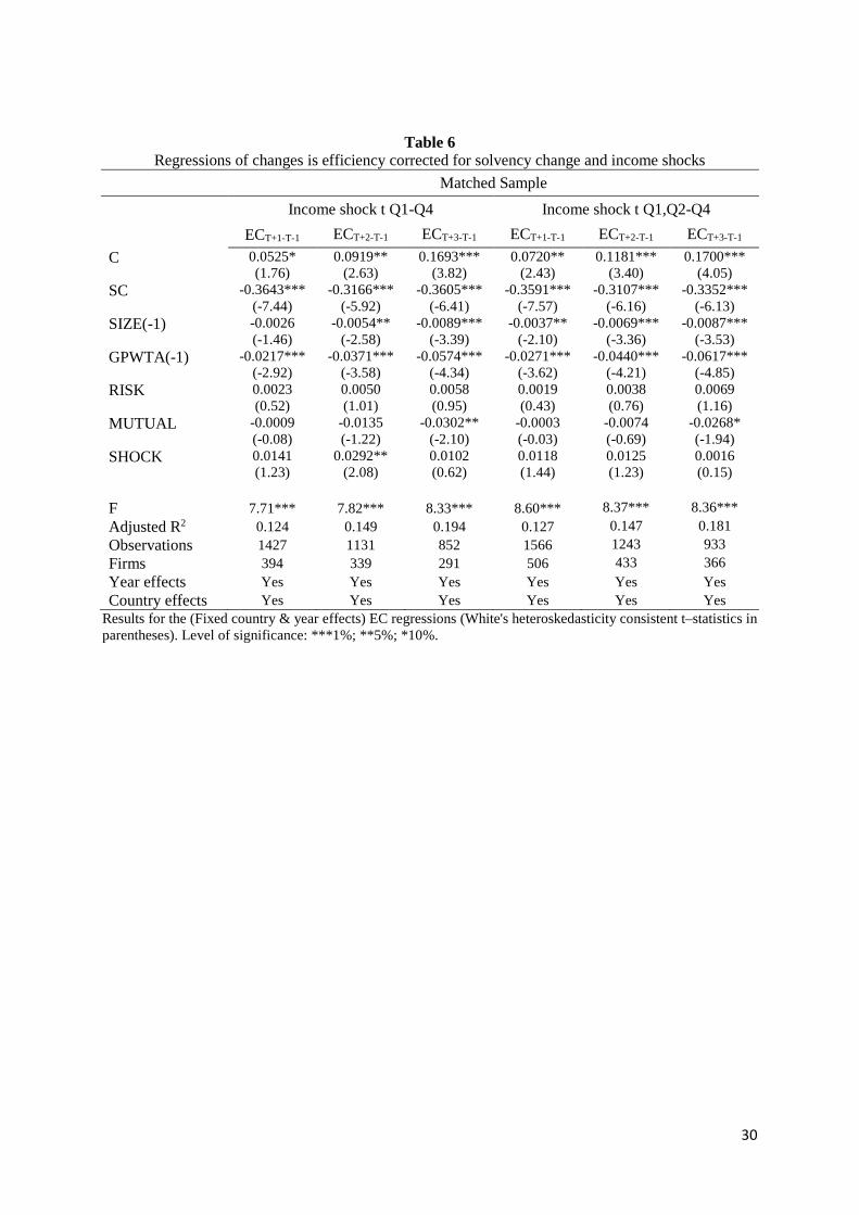
Due to the potential influence of solvency changes on the resulting efficiency change following

an income shock, we re-estimate the basic model again replacing the level of solvency with the

solvency change (SC) over the corresponding window used for the efficiency change. Results

are reported in Table 6 for matched samples only. In line with our expectations based on the

business cycle literature, solvency changes play an important role in the efficiency change

following the shock as the SC coefficient is significantly negative for all models in Table 6.

Strong decreases in surplus, holding the other inputs and outputs constant, would be beneficial

for efficiency increases. This proves that to some extent, all insurers profit from the flexibility

inherent in their business model. As long as profitability restores in the following years, insurers

can slowly rebuilt their capital structure (Weiss, 2007). Therefore in line with our univariate

19

results, the efficiency increase following an income shock can be partly explained by the

resulting drop in solvency. As a result, the coefficient for the income shock itself no longer

seems significant once the solvency change is taken into account. However, not all insurers will

be able to fully exploit this solvency channel because of the risk of losing business. In order to

test our second hypothesis, we split up the coefficient of income shock depending on the

opaqueness dimensions described above.

20

Influence of opaqueness on efficiency changes

In order to test our second hypothesis, we estimate the regression models of Table 6 introducing

the opaqueness measures (OQ). Table 7 and table 8 report the regressions on the impact of our

two income shock measures respectively over the two year window (ECT+2-T-1). Each model has

a different opaqueness dummy (OQ) that separates the shock dummy based on the opaqueness

subsamples. Interestingly, while the effect of the opaqueness dummy itself on efficiency

changes is not always the same across regression models, its interaction with the shock dummy

is consistently positive. This means that our results strongly support the hypothesis that insurers

that are characterised as more opaque, show stronger reactions to income shocks. For the

subsamples where opaqueness is expected to be minor (1-OQ), the income shock did not trigger

significant efficiency change beyond the change in solvency (SC). This proves that insurers that

are deemed more opaque will have to restructure more quickly as they lack the flexibility of

letting the profitability gradually restore the capital buffers. This can also explain why we found

a stronger increase in efficiency for these latter firms but a relatively smaller decrease in

solvency. Profitability would therefore have to be increased to avoid enhanced scrutiny by

policy holders and potential loss of business. Note that even the result based on the

capitalisation measure of opaqueness is no longer counter intuitive. Once controlled for the

opportunities of solvency change, low capitalised forms seem to react more strongly on a shock

in profitability compared to insurers with solvency ratios well above the minimum required

levels. In sum, Tables 7 and 8 provide strong evidence that opaqueness pressures insurers to

restore performance more rapidly in order to avoid that income shocks are perceived as signals

of bad financial soundness causing loss of reputation and customer business.

As a final test of insurance opacity, Table 9 reports results from the regressions where the shock

dummy is split up depending on the organizational characteristics. As explained above, mutual

insurers as well as unlisted insurers are expected to be harder to evaluate due to limited

disclosure rules compared to either stock companies in general or listed companies in particular.

However, as a very limited number of the insurance firms are listed, the subsample of listed

insurers that experience an income shock maybe is too small to generate meaningful results.

Nevertheless, both the unlisted and mutual insurers show an increased reaction to an income

shock which is in line with our opaqueness hypothesis, although the difference is only

significant for mutual insurers.

21

Conclusion

This article examines the reaction of non life insurance companies to an income shock on a

sample of European insurers over the period 2003-2013. We contribute to both the corporate

finance as well as insurance literature by (first) providing evidence on how the difference in

business model between insurers and non financial companies shapes the restructuring process

and (second) evaluate the role of opaqueness which is typical for financial services companies

in general and the insurance industry in particular.

As for insurance companies, unlike non-financial firms, upfront financing of vast amounts of

fixed assets and working capital are not an issue due to the inverse cash cycle, restructuring

following loss events is not aimed at cash conservation and improvement of efficiency to

enhance future cash generation capacity. However, this does not mean that insurers are immune

to income shocks. Although the solvency buffer will partly absorb the income shock (not all)

insurers can’t fully exploit the flexibility offered by business cycles and would still feel

pressured to actively react upon a setback. This is due to the so called flight to quality risk due

to the fact that policy holders are unable to fully assess the impact of a particular shock to future

financial soundness of the insurance company. We show that for this reason insurers experience

an increase in efficiency scores in the years following the income shock.

We find however, that a big portion of the efficiency increase is represented by the temporary

reduction in solvency indicating the above mentioned exploitation of flexibility offered by the

insurers’ business model. When the decrease of the solvency buffer is taken into account, an

interesting picture emerges. Only the insurers with high levels of our proxies for opaqueness

(e.g., reinsurance, income and product uncertainty, long tail business,…) increase productivity

significantly compared to matched non shock firms. This strongly indicates that these more

opaque insurers are pressured to restore performance more rapidly by increasing efficiency

beyond the solvency change. Our results therefore prove that the determinants of insurer

opaqueness strongly influence the reaction to an income shock.

While our results provide compelling evidence on the role of insurer opaqueness on

restructuring in the insurance industry, there is sufficient room for improvement or avenues for

future research. First, our research methodology could be elaborated to include other efficiency

statistics (e.g., data envelopment analysis) and or income shock definitions. Additionally, we

could assess whether the financial health ratings themselves influence our story. Finally, an

22

interesting avenue for further research would be the decomposition of resulting efficiency

scores.

References

Adamson, S. R., Eckles, D. L., & Haggard, K. S. (2014). Insurer Opacity and Ownership Structure. Journal of Insurance Issues, 93-134.

Babbel, D. F., & Merrill, C. (2005). Real and illusory value creation by insurance companies. Journal of Risk and Insurance, 72(1), 1-22.

Baranoff, E. G., and Sager, T. W. (2007), Market Discipline in Life Insurance: Insureds’ Reaction to Rating Downgrades in the Context of Enterprise Risks, Working Paper.

Bertoni, F., & Croce, A. (2011). The productivity of European life insurers: best-practice adoption vs. innovation. The Geneva Papers on Risk and Insurance-Issues and Practice, 36(2), 165-185.

Boubakri, N. (2011). Corporate governance and issues from the insurance industry. Journal of Risk and Insurance, 78(3), 501-518.

Chen, L. R., Lai, G. C., & Wang, J. L. (2011). Conversion and efficiency performance changes: Evidence from the US property-liability insurance industry. The Geneva Risk and Insurance Review, 36(1), 1-35.

Cole, C. R., He, E., McCullough, K. A., Semykina, A., & Sommer, D. W. (2011). An empirical examination of stakeholder groups as monitoring sources in corporate governance. Journal of Risk and Insurance, 78(3), 703-730.

Cummins, J. D., & Lewis, C. M. (2003). Catastrophic events, parameter uncertainty and the breakdown of implicit long-term contracting: The case of terrorism insurance. In The Risks of Terrorism (pp. 55-80). Springer US.

Cummins, J. D., & Weiss, M. A. (2013). Analyzing firm performance in the insurance industry using frontier efficiency and productivity methods. In Handbook of insurance (pp. 795-861). Springer New York.

Cummins, J. D., & Xie, X. (2008). Mergers and acquisitions in the US property-liability insurance industry: Productivity and efficiency effects. Journal of Banking & Finance, 32(1), 30-55.

Cummins, J.D. and Danzon, P.M. (1997) Price, financial quality, and capital flows in insurance markets. Journal of Financial Intermediation 6(1): 3-38.

De Haan, L. and Kakes, J. (2010) Are non-risk based capital requirements for insurance companies binding?. Journal of Banking and Finance 34(7): 1618-1627.

Denis, D. J., & Kruse, T. A. (2000). Managerial discipline and corporate restructuring following performance declines. Journal of Financial Economics, 55(3), 391-424.

Dhaene, J., Van Hulle, C., Wuyts, G., Schoubben, F., & Schoutens, W. (2015). Is the capital structure logic of corporate finance applicable to insurers? Review and analysis. Journal of Economic Surveys. (Article first published online : 22 AUG 2015), 1-21.

Doherty, N.A. and Phillips, R. (2002) Keeping up with the Joneses: changing rating standards and the buildup of capital by U.S. property-liability insurers. Journal of Financial Services Research 21(1-2): 55-76.

23

Doherty, N.A. and Phillips, R. (2002) Keeping up with the Joneses: changing rating standards and the buildup of capital by U.S. property-liability insurers. Journal of Financial Services Research 21(1-2): 55-76.

Doherty, N.A. and Posey, L. (1997) Availability crises in insurance markets: Optimal contracts with asymmetric information and capacity constraints. Journal of Risk and Uncertainty 15(1): 55-80.

Eckles, D. L., & Pottier, S. W. (2011). Is Efficiency an Important Determinant of AM Best Property-Liability Insurer Financial Strength Ratings?. Journal of Insurance Issues, 18-33.

Eling, M. (2012). What do we know about market discipline in insurance?. Risk Management and Insurance Review, 15(2), 185-223.

Eling, M., & Luhnen, M. (2010). Frontier efficiency methodologies to measure performance in the insurance industry: overview, systematization, and recent developments. The Geneva Papers on Risk and Insurance-Issues and Practice, 35(2), 217-265.

Eling, M., & Marek, S. D. (2014). Corporate governance and risk taking: Evidence from the UK and German insurance markets. Journal of Risk and Insurance, 81(3), 653-682.

Eling, M., & Schmit, J. T. (2012). Is There Market Discipline in the European Insurance Industry&quest; An Analysis of the German Insurance Market. The Geneva Risk and Insurance Review, 37(2), 180-207.

Epermanis, K., & Harrington, S. E. (2000, February). Financial Rating Changes and Market Discipline in Property-Liability Insurance. In Risk Theory Society Meeting.

Epermanis, K., & Harrington, S. E. (2006). Market discipline in property/casualty insurance: Evidence from premium growth surrounding changes in financial strength ratings. Journal of Money, Credit and Banking, 1515-1544.

Fenn, P., Vencappa, D., Diacon, S., Klumpes, P., & O’Brien, C. (2008). Market structure and the efficiency of European insurance companies: a stochastic frontier analysis. Journal of Banking & Finance, 32(1), 86-100.

Fenn, P., Vencappa, D., Diacon, S., Klumpes, P., & O’Brien, C. (2008). Market structure and the efficiency of European insurance companies: a stochastic frontier analysis. Journal of Banking & Finance, 32(1), 86-100.

Fields, L. P., Gupta, M., & Prakash, P. (2012). Risk taking and performance of public insurers: An international comparison. Journal of Risk and Insurance, 79(4), 931-962.

Figlewski, S., Frydman, H., & Liang, W. (2012). Modeling the effect of macroeconomic factors on corporate default and credit rating transitions. International Review of Economics & Finance, 21(1), 87-105.

Flannery, M. J. (2001). The faces of “market discipline”. Journal of Financial Services Research, 20(2-3), 107-119.

Hagendorff, B., Hagendorff, J., & Keasey, K. (2015). The Impact of Mega‐Catastrophes on Insurers: An Exposure‐Based Analysis of the US Homeowners’ Insurance Market. Risk Analysis, 35(1), 157-173.

Halek, M., & Eckles, D. L. (2010). Effects of analysts’ ratings on insurer stock returns: evidence of asymmetric responses. Journal of Risk and Insurance, 77(4), 801-827.

Harrington, S. E., & Niehaus, G. (2002). Capital structure decisions in the insurance industry: stocks versus mutuals. Journal of Financial Services Research, 21(1-2), 145-163.

He, E., Sommer, D. W., & Xie, X. (2011). The Impact of CEO Turnover on Property–Liability Insurer Performance. Journal of Risk and Insurance, 78(3), 583-608.

Ho, C. L., Lai, G. C., & Lee, J. P. (2013). Organizational structure, board composition, and risk taking in the US property casualty insurance industry. Journal of Risk and Insurance, 80(1), 169-203.

24

Huang, W., & Eling, M. (2013). An efficiency comparison of the non-life insurance industry in the BRIC countries. European Journal of Operational Research, 226(3), 577-591.

John, K., Lang, L. H., & Netter, J. (1992). The voluntary restructuring of large firms in response to performance decline. The Journal of Finance, 47(3), 891-917.

Kang, J. K., & Shivdasani, A. (1997). Corporate restructuring during performance declines in Japan. Journal of Financial Economics, 46(1), 29-65.

Laeven, L., & Levine, R. (2009). Bank governance, regulation and risk taking. Journal of Financial Economics, 93(2), 259-275.

Morgan, D. P. (2000). Rating banks: Risk and uncertainty in an opaque industry. FRB of New York Staff Report, (105).

Morgan, D. P., 2002, Rating Banks: Risk and Uncertainty in an Opaque Industry, American Economic Review, 92: 874-888.

Ofek, E. (1993). Capital structure and firm response to poor performance: An empirical analysis. Journal of financial economics, 34(1), 3-30.

Pasiouras, F., & Gaganis, C. (2013). Regulations and soundness of insurance firms: International evidence. Journal of Business Research, 66(5), 632-642.

Petroni, K. R., 1992, Optimistic Reporting in the Property–Casualty Insurance Industry, Journal of Accounting and Economics, 15: 485-508. Pottier, S. W., & Sommer, D. W. (2006). Opaqueness in the insurance industry: Why are some

insurers harder to evaluate than others?. Risk Management and Insurance Review, 9(2), 149-163.

Schoenberg, R., Collier, N., & Bowman, C. (2013). Strategies for business turnaround and recovery: a review and synthesis. European Business Review, 25(3), 243-262.

Shim, J. (2010) Capital-based regulation, portfolio risk and capital determination: Empirical evidence from the U.S. property-liability insurers. Journal of Banking and Finance 34(10): 2450-2461.

Shim, J. (2015). AN INVESTIGATION OF MARKET CONCENTRATION AND FINANCIAL STABILITY IN PROPERTY–LIABILITY INSURANCE INDUSTRY. Journal of Risk and Insurance.

Singh, A. K., & Power, M. L. (1992). The effects of Best's rating changes on insurance company stock prices. Journal of Risk and Insurance, 310-317.

Swiss Re Sigma (2014) World insurance in 2013: steering towards recovery. Swiss RE Sigma 3: 1-45.

Vencappa, D., Fenn, P., & Diacon, S. (2013). Productivity Growth in the European Insurance Industry: Evidence from Life and Non-Life Companies. International Journal of the Economics of Business, 20(2), 281-305.

Vencappa, D., Fenn, P., Diacon, S., & Campus, J. (2008). Parametric decomposition of total factor productivity growth in the European insurance industry: evidence from life and non-life companies. working paper, Nottingham University.

Wang, Y., & Carson, J. M. (2014). Rating Drift in Property-Liability Insurer Rating Transitions. The Journal of Insurance ISSUES, 59-76.

Weiss, M. A. (2007). Underwriting cycles: a synthesis and further directions. Journal of Insurance Issues, 31-45.

Zhang, T., Cox, L. A., & Van Ness, R. A. (2009). Adverse selection and the opaqueness of insurers. Journal of Risk and Insurance, 76(2), 295-321.

25

Table 1

Country/yearly differences in efficiency scores and income shocks

Panel A SFA efficiency scores Income shocks

Countries Firm years mean median Q1-Q4 Q1,2-Q4

Austria 137 0.6451 0.6700 0.73% 2.19%

Belgium 339 0.5822 0.6411 0.59% 3.83%

Bulgaria 131 0.5387 0.6160 2.29% 3.05%

Czech Rep. 174 0.4796 0.4989 2.30% 3.45%

Denmark 314 0.6242 0.6622 1.59% 5.41%

France 1117 0.6455 0.6814 0.54% 2.24%

Germany 2444 0.5817 0.6118 1.60% 3.89%

Ireland 340 0.5694 0.6248 2.94% 7.65%

Italy 646 0.5825 0.6444 0.93% 2.48%

Luxembourg 273 0.6245 0.6589 1.47% 2.56%

Netherlands 510 0.6710 0.6828 2.35% 6.47%

Norway 122 0.5633 0.6327 2.46% 4.10%

Poland 131 0.6972 0.7159 0.00% 3.05%

Russia 452 0.6334 0.6963 0.89% 3.54%

Spain 853 0.6724 0.7134 0.82% 1.99%

Sweden 293 0.5806 0.6147 4.44% 11.60%

Switzerland 953 0.6247 0.6678 0.52% 2.83%

Turkey 186 0.6620 0.7049 1.08% 5.38%

UK 2074 0.5854 0.6326 2.36% 6.17%

Full Sample 11489 0.6079 0.6450 1.52% 4.23%

Panel B SFA efficiency scores Income shocks

Years Firms mean median Q1-Q4 Q1,2-Q4

2003 596 / / / /

2004 685 / / 1.46% 3.07%

2005 721 0.6051 0.6341 1.39% 4.99%

2006 834 0.5906 0.6288 1.08% 4.08%

2007 913 0.6005 0.6397 0.88% 2.96%

2008 1137 0.5917 0.6238 3.17% 7.30%

2009 1208 0.6093 0.6416 1.66% 4.88%

2010 1279 0.6105 0.6478 1.02% 2.81%

2011 1402 0.6092 0.6479 2.50% 6.35%

2012 1454 0.6161 0.6512 1.38% 4.13%

2013 1260 0.6273 0.6622 1.11% 3.25%

Full Sample 11489 0.6079 0.6450 1.52% 4.23%

26

Table 2

Summary statistics of variables used

mean median Stdev min max

Inputs & outputs (Millions)

Gross claims 294 46 987 0 24678

Gross technical reserves 779 96 3097 0 65023

Equity capital 391 45 2405 0 87948

Underwriting expenses 553 68 2434 0 89702

Independent variables

SOLV 0.38 0.34 0.22 0.00 1.00

SIZE 11.99 11.95 2.05 5.20 21.65

GPWTA 0.60 0.50 0.50 0.00 2.23

RISK 1.13 1.16 0.90 -7.71 4.52

Opaqueness Measures

Reinsurance 0.55 1.00 0.50 0 1

Income uncertainty 0.33 0.00 0.50 0 1

Business uncertainty 0.31 0.00 0.47 0 1

Long tail business 0.24 0.00 0.46 0 1

Small insurer 0.32 0.00 0.47 0 1

Low capitalization 0.145 0 0.35 0 1

Mutual 0.12 0.00 0.32 0 1

Unlisted insurer 0.97 1 0.17 0 1

27

Table 3

Univariate statistics on efficiency change following income shocks

Panel A Full sample Shock: Q1-Q4

Shock: Q1,Q2-Q4

No shock No shock (matched)

Efficiency change (ECT+1-T-1)

Meana 0.0103 0.0358** 0.0317*** 0.0094 0.0067 Medianb 0.0066 0.0300*** 0.0154*** 0.0065 0.0064

Efficiency change

(ECT+2-T-1) Mean 0.0118 0.0455*** 0.0287** 0.0100 0.0071

Median 0.0056 0.0234*** 0.0164*** 0.0043 0.0028

Efficiency change (ECT+3-T-1)

Mean 0.0160 0.0352* 0.0197 0.0141 0.0133 Median 0.0094 0.0235** 0.0110 0.0086 0.0074

aTest of the mean EC difference between shock and (matched) non shock firms based on student t test bTest of median difference between shock and (matched) non shock firms based on Wilcoxon Mann–Whitney test cTest of the mean EC difference based on opaqueness within shock firms based on student t test *Level of significance: ***1%; **5%; *10%.

Panel B High Opaquenessc Low Opaqueness

ECT+1-T-1 ECT+2-T-1 ECT+3-T-1 ECT+1-T-1 ECT+2-T-1 ECT+3-T-1

Shock: Q1-Q4

Reinsurance 0.0432* 0.0532 0.0464* 0.0170 0.0273 0.0064

Income uncertainty 0.0450** 0.0591** 0.0425* 0.0081 0.0038 0.0183

Business uncertainty 0.0481* 0.0719*** 0.0481** 0.0207 0.0154 0.0188

Long tail business 0.0549* 0.0952*** 0.0805*** 0.0271 0.0229 0.0158

Small insurer 0.0566* 0.0577* 0.0400* 0.0233 0.0380 0.0315

Mutual 0.0343 0.0450 0.0213 0.0363 0.0456 0.0387

Listing 0.0326 0.0435 0.0322 0.1087 0.0935 0.0812

Low capitalization 0.0030* 0.0090** 0.0258 0.0434 0.0543 0.0373

Shock: Q1,Q2-Q4

Reinsurance 0.0328* 0.0283 0.0315** 0.0292 0.0296 -0.0058

Income uncertainty 0.0371* 0.0439* 0.0321** 0.0226 0.0035 0.0018

Business uncertainty 0.0530** 0.0585*** 0.0352*** 0.0143 0.0067 0.0093

Long tail business 0.0539** 0.0469** 0.0963*** 0.0240 0.0230 -0.0010

Small insurer 0.0424 0.0328 0.0081 0.0267 0.0268 0.0256

Mutual 0.0159 0.0265 0.0008 0.0358 0.0294 0.0238

Listing 0.0313 0.0289 0.0192 0.0449 0.0205 0.0403

Low capitalization 0.0089* 0.0109* 0.0091** 0.0344 0.0312 0.0211

28

Table 4

Univariate statistics on solvency change following income shocks

Panel A Full sample Shock: Q1-Q4

Shock: Q1,Q2-Q4

No shock No shock (matched)

Solvency change (SCT+1-T-1)

Meana 0.0024 -0.0292*** -0.0345*** 0.0022 0.0037 Medianb 0.0041 -0.0339*** -0.0290*** 0.0047 0.0036

Solvency change

(SCT+2-T-1) Mean 0.0047 -0.0394*** -0.0325*** 0.0056 0.0066

Median 0.0055 -0.0316*** -0.0211*** 0.0063 0.0056

Solvency change (SCT+3-T-1)

Mean 0.0068 -0.0439*** -0.0344*** 0.0088 0.0090 Median 0.0062 -0.0388*** -0.0251*** 0.0080 0.0056

aTest of the mean SC difference between shock and (matched) non shock firms based on student t test bTest of median difference between shock and (matched) non shock firms based on Wilcoxon Mann–Whitney test cTest of the mean SC difference based on opaqueness within shock firms based on student t test *Level of significance: ***1%; **5%; *10%.

Panel B High Opaquenessc Low Opaqueness

SCT+1-T-1 SCT+2-T-1 SCT+3-T-1 SCT+1-T-1 SCT+2-T-1 SCT+3-T-1

Shock: Q1-Q4

Reinsurance -0.0229 -0.0150** -0.0253* -0.0349 -0.0600 -0.0597

Income uncertainty -0.0244 -0.0291* -0.0346* -0.0433 -0.0732 -0.0712

Business uncertainty -0.0230 -0.0298 -0.0430 -0.0370 -0.0510 -0.0450

Long tail business -0.0030 -0.0074* -0.0469 -0.0398 -0.0520 -0.0427

Small insurer -0.0410 -0.0520 -0.0681 -0.0217 -0.0313 -0.0233

Mutual -0.0249 -0.0124 -0.0748 -0.0304 -0.0488 -0.0364

Listing -0.0261 -0.0368 -0.0405 -0.1385 -0.1413 -0.1382

Low capitalization -0.0252 -0.0125* -0.0298* -0.0298 -0.0435 -0.0461

Shock: Q1,Q2-Q4

Reinsurance -0.0372 -0.0286 -0.0379 -0.0315 -0.0371 -0.0299

Income uncertainty -0.0302 -0.0303 -0.0316 -0.0408 -0.0357 -0.0383

Business uncertainty -0.0360 -0.0307 -0.0415 -0.0332 -0.0341 -0.0277

Long tail business -0.0212 -0.0144 -0.0391 -0.0393 -0.0388 -0.0328

Small insurer -0.0470 -0.0595 -0.0532 -0.0287 -0.0204 -0.0254

Mutual -0.0208 -0.0110 -0.0360 -0.0373 -0.0375 -0.0342

Listing -0.0337 -0.0319 -0.0332 -0.0685 -0.0539 -0.0838

Low capitalization -0.0056* 0.0027** 0.0230*** -0.0387 -0.0376 -0.0431

29

Table 5 Regressions of changes is efficiency and income shocks

Panel A Income shock t Q1-Q4

Full Sample* Matched Sample


C -0.0063 (-0.31)

0.0060 (0.26)

0.0280 (1.00)

-0.0195 (-0.62)

0.0016 (0.05)

0.0564 (1.37)

SOLV(-1) 0.0603*** (5.17)

0.0758*** (5.20)

0.0766*** (3.89)

0.1389*** (5.72)

0.1605*** (5.15)

0.1979*** (5.57)

SIZE(-1) -0.0006 (-0.50)

-0.0020 (-1.53)

-0.0031* (-1.94)

0.0006 (0.30)

-0.0013 (-0.63)

-0.0039 (-1.57)

GPWTA(-1) -0.0247*** (-4.42)

-0.0348*** (-5.76)

-0.0464*** (-5.65)

-0.0233*** (-3.06)

-0.0375*** (-3.74)

-0.0578*** (-4.53)

RISK 0.0044* (1.67)

0.0083** (2.61)

0.0102** (2.39)

-0.0048 (-1.01)

-0.0036 (-0.63)

-0.0048 (-0.68)

MUTUAL -0.0073 (-1.18)

-0.0144** (-2.11)

-0.0178** (-2.11)

-0.0075 (-0.64)

-0.0216* (-1.85)

-0.0407** (-2.66)

SHOCK 0.0255*** (2.54)

0.0360*** (2.95)

0.0218 (1.50)

0.0163* (1.65)

0.0290** (2.10)

0.0083 (0.52)

F 7.93*** 9.90*** 9.15*** 4.59*** 5.84*** 6.18*** Adjusted R2 0.054 0.083 0.096 0.070 0.110 0.145 Observations 3619 2841 2146 1427 1131 852 Firms 918 794 709 394 339 291 Year effects Yes Yes Yes Yes Yes Yes Country effects Yes Yes Yes Yes Yes Yes

Panel B Income shock t Q1,Q2-Q4

Full Sample* Matched Sample


C -0.0021 (-0.11)

0.0118 (0.52)

0.0250 (0.91)

0.0014 (0.05)

0.0285 (0.86)

0.0633 (1.61)

SOLV(-1) 0.0598*** (5.23)

0.0743*** (5.21)

0.0736*** (3.84)

0.1362*** (5.89)

0.1583*** (5.21)

0.1874*** (5.51)

SIZE(-1) -0.0008 (-0.70)

-0.0024* (-1.82)

-0.0028* (-1.76)

-0.0006 (-0.34)

-0.0030 (-1.47)

-0.0040* (-1.68)

GPWTA(-1) -0.0266*** (-4.85)

-0.0372*** (-6.26)

-0.0476*** (-5.91)

-0.0288*** (-3.73)

-0.0438*** (-4.31)

-0.0629*** (-5.01)

RISK 0.0047* (1.79)

0.0088** (2.76)

0.0109** (2.60)

-0.0051 (-1.10)

-0.0044 (-0.77)

-0.0032 (-0.47)

MUTUAL -0.0089 (-1.45)

-0.0142** (-2.08)

-0.0185** (-2.25)

-0.0077 (-0.69)

-0.0162 (-1.41)

-0.0391*** (-2.72)

SHOCK 0.0235*** (3.12)

0.0212** (2.21)

0.0068 (0.69)

0.0163* (1.93)

0.0150* (1.95)

0.0018 (0.17)

F 8.59 10.24 9.53 5.39 6.26 6.44 Adjusted R2 0.057 0.082 0.096 0.078 0.109 0.141 Observations 3791 2981 2248 1566 1243 933 Firms 1061 914 804 506 433 366 Year effects Yes Yes Yes Yes Yes Yes Country effects Yes Yes Yes Yes Yes Yes

Results for the (Fixed country & year effects) EC regressions (White's heteroskedasticity consistent t–statistics in parentheses). Level of significance: ***1%; **5%; *10%.

30

Table 6 Regressions of changes is efficiency corrected for solvency change and income shocks

Matched Sample

Income shock t Q1-Q4 Income shock t Q1,Q2-Q4


C 0.0525* (1.76)

0.0919** (2.63)

0.1693*** (3.82)

0.0720** (2.43)

0.1181*** (3.40)

0.1700*** (4.05)

SC -0.3643*** (-7.44)

-0.3166*** (-5.92)

-0.3605*** (-6.41)

-0.3591*** (-7.57)

-0.3107*** (-6.16)

-0.3352*** (-6.13)

SIZE(-1) -0.0026 (-1.46)

-0.0054** (-2.58)

-0.0089*** (-3.39)

-0.0037** (-2.10)

-0.0069*** (-3.36)

-0.0087*** (-3.53)

GPWTA(-1) -0.0217*** (-2.92)

-0.0371*** (-3.58)

-0.0574*** (-4.34)

-0.0271*** (-3.62)

-0.0440*** (-4.21)

-0.0617*** (-4.85)

RISK 0.0023 (0.52)

0.0050 (1.01)

0.0058 (0.95)

0.0019 (0.43)

0.0038 (0.76)

0.0069 (1.16)

MUTUAL -0.0009 (-0.08)

-0.0135 (-1.22)

-0.0302** (-2.10)

-0.0003 (-0.03)

-0.0074 (-0.69)

-0.0268* (-1.94)

SHOCK 0.0141 (1.23)

0.0292** (2.08)

0.0102 (0.62)

0.0118 (1.44)

0.0125 (1.23)

0.0016 (0.15)



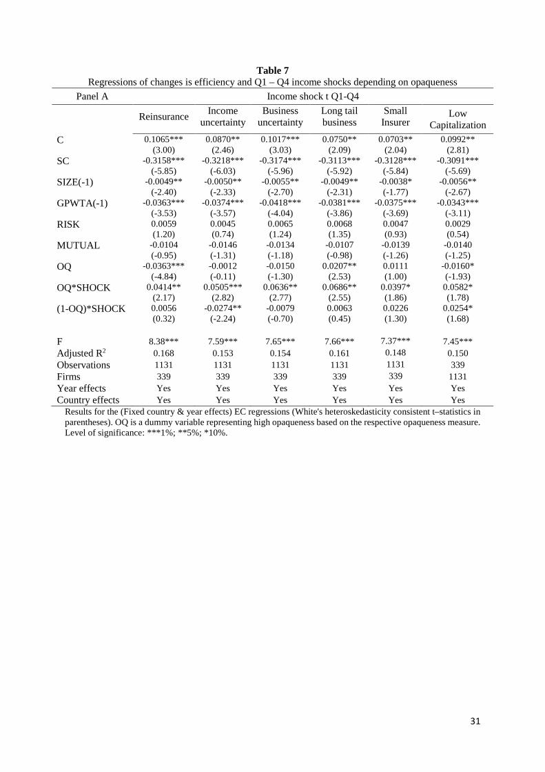
31

Table 7 Regressions of changes is efficiency and Q1 – Q4 income shocks depending on opaqueness

Panel A Income shock t Q1-Q4

Reinsurance Income

uncertainty Business

uncertainty Long tail business

Small Insurer

Low Capitalization

C 0.1065*** (3.00)

0.0870** (2.46)

0.1017*** (3.03)

0.0750** (2.09)

0.0703** (2.04)

0.0992** (2.81)

SC -0.3158*** (-5.85)

-0.3218*** (-6.03)

-0.3174*** (-5.96)

-0.3113*** (-5.92)

-0.3128*** (-5.84)

-0.3091*** (-5.69)

SIZE(-1) -0.0049** (-2.40)

-0.0050** (-2.33)

-0.0055** (-2.70)

-0.0049** (-2.31)

-0.0038* (-1.77)

-0.0056** (-2.67)

GPWTA(-1) -0.0363*** (-3.53)

-0.0374*** (-3.57)

-0.0418*** (-4.04)

-0.0381*** (-3.86)

-0.0375*** (-3.69)

-0.0343*** (-3.11)

RISK 0.0059 (1.20)

0.0045 (0.74)

0.0065 (1.24)

0.0068 (1.35)

0.0047 (0.93)

0.0029 (0.54)

MUTUAL -0.0104 (-0.95)

-0.0146 (-1.31)

-0.0134 (-1.18)

-0.0107 (-0.98)

-0.0139 (-1.26)

-0.0140 (-1.25)

OQ -0.0363*** (-4.84)

-0.0012 (-0.11)

-0.0150 (-1.30)

0.0207** (2.53)

0.0111 (1.00)

-0.0160* (-1.93)

OQ*SHOCK 0.0414** (2.17)

0.0505*** (2.82)

0.0636** (2.77)

0.0686** (2.55)

0.0397* (1.86)

0.0582* (1.78)

(1-OQ)*SHOCK 0.0056 (0.32)

-0.0274** (-2.24)

-0.0079 (-0.70)

0.0063 (0.45)

0.0226 (1.30)

0.0254* (1.68)


Results for the (Fixed country & year effects) EC regressions (White's heteroskedasticity consistent t–statistics in parentheses). OQ is a dummy variable representing high opaqueness based on the respective opaqueness measure. Level of significance: ***1%; **5%; *10%.

32

Table 8 Regressions of changes is efficiency and Q1,Q2 – Q4 income shocks depending on opaqueness

Panel B Income shock t Q1,Q2-Q4

Reinsurance Income

uncertainty Business

uncertainty Long tail business

Small Insurer

Low Capitalization

C 0.1232*** (3.92)

0.1175*** (3.75)

0.1298*** (4.07)

0.1016*** (3.20)

0.1086*** (2.98)

0.1251*** (3.98)

SC -0.3131*** (-10.33)

-0.3105*** (-10.28)

-0.3085*** (-10.24)

-0.3048*** (-10.08)

-0.3089*** (-10.17)

-0.0030*** (-9.87)

SIZE(-1) -0.0068*** (-3.45)

-0.0068*** (-3.39)

-0.0072*** (-3.63)

-0.0065*** (-3.26)

-0.0062** (-2.58)

-0.0072*** (-3.61)

GPWTA(-1) -0.0435*** (-4.91)

-0.0447*** (-4.98)

-0.0495*** (-5.41)

-0.0437*** (-4.97)

-0.0444*** (-4.96)

-0.0394*** (-4.26)

RISK 0.0040 (0.90)

0.0035 (0.60)

0.0052 (1.17)

0.0053 (1.19)

0.0037 (0.84)

0.0016 (0.36)

MUTUAL -0.0069 (-0.63)

-0.0079 (-0.72)

-0.0061 (-0.56)

-0.0046 (-0.42)

-0.0076 (-0.69)

-0.0073 (-0.67)

OQ -0.0111 (-1.55)

-0.0032 (-0.30)

-0.0182** (-2.20)

0.0203** (2.66)

0.0042 (0.37)

-0.0176** (-2.06)

OQ*SHOCK 0.0161* (1.85)

0.0272** (2.22)

0.0459*** (3.33)

0.0263* (1.62)

0.0183 (1.04)

0.0392** (2.15)

(1-OQ)*SHOCK 0.0060 (0.37)

-0.0061 (-0.46)

-0.0101 (-0.87)

0.0066 (0.64)

0.0106 (1.02)

0.0093 (0.99)


Results for the (Fixed country & year effects) EC regressions (White's heteroskedasticity consistent t–statistics in parentheses). OQ is a dummy variable representing high opaqueness based on the respective opaqueness measure. Level of significance: ***1%; **5%; *10%.

33

Table 9 Regressions of changes is efficiency and income shocks depending on ownership

Income shock t Q1-Q4 Income shock t Q1,Q2-Q4

Unlisted Mutual Unlisted Mutual

C 0.0891** (2.57)

0.0927** (2.65)

0.1144*** (3.62)

0.1208*** (3.87)

SC -0.3162*** (-5.89)

-0.3166*** (-5.92)

-0.0031*** (-10.28)

-0.3109*** (-10.29)

SIZE(-1) -0.0051** (-2.46)

-0.0054** (-2.58)

-0.0066*** (-3.26)

-0.0070*** (-3.53)

GPWTA(-1) -0.0369*** (-3.56)

-0.0377*** (-3.62)

-0.0438*** (-4.95)

-0.0450*** (-5.09)

RISK 0.0050 (1.01)

0.0051 (1.01)

0.0038 (0.86)

0.0036 (0.83)

MUTUAL (M) -0.0135 (-1.22)

-0.0178 (-1.50)

-0.0076 (-0.69)

-0.0186 (-1.46)

Unlisted (UL) -0.0099 (-0.73)

/ -0.0112 (-0.62)

/

UL*SHOCK 0.0284* (1.98)

/ 0.0127 (1.36)

/

(1-UL)*SHOCK 0.0504 (0.94)

/ 0.0083 (0.19)

/

M*SHOCK / 0.0477* (1.77)

/ 0.0451**

(2.14) (1-M)*SHOCK /

0.0226 (1.46)

/ 0.0061 (0.62)

F 7.32*** 7.58*** 7.34*** 8.20*** Adjusted R2 0.148 0.101 0.146 0.104 Observations 1131 1131 1243 1243 Firms 339 339 433 433 Year effects Yes Yes Yes Yes Country effects Yes Yes Yes Yes


draft opaqueness income shocks - EFMA ANNUAL MEETINGS/2016-… · income shocks Frederiek Schoubben...

Documents

Transcript of draft opaqueness income shocks - EFMA ANNUAL MEETINGS/2016-… · income shocks Frederiek Schoubben...