DQM: Decentralized Quadratically ApproximatedAlternating Direction Method of Multipliers

Aryan Mokhtari, Wei Shi, Qing Ling, and Alejandro Ribeiro

Abstract—This paper considers decentralized consensus optimiza-tion problems where nodes of a network have access to differentsummands of a global objective function. Nodes cooperate to mini-mize the global objective by exchanging information with neighborsonly. A decentralized version of the alternating directions methodof multipliers (DADMM) is a common method for solving thiscategory of problems. DADMM exhibits linear convergence rate tothe optimal objective but its implementation requires solving a convexoptimization problem at each iteration. This can be computationallycostly and may result in large overall convergence times. Thedecentralized quadratically approximated ADMM algorithm (DQM),which minimizes a quadratic approximation of the objective functionthat DADMM minimizes at each iteration, is proposed here. Theconsequent reduction in computational time is shown to have minimaleffect on convergence properties. Convergence still proceeds at a lin-ear rate with a guaranteed constant that is asymptotically equivalentto the DADMM linear convergence rate constant. Numerical resultsdemonstrate advantages of DQM relative to DADMM and otheralternatives in a logistic regression problem.

Index Terms—Multi-agent network, decentralized optimization,Alternating Direction Method of Multipliers.

I. INTRODUCTION

Decentralized algorithms are used to solve optimization prob-lems where components of the objective are available at differentnodes of a network. Nodes access their local cost functions onlybut try to minimize the aggregate cost by exchanging informationwith their neighbors. Specifically, consider a variable x ∈ Rp anda connected network containing n nodes each of which has accessto a local cost function fi : Rp → R. The nodes’ goal is to findthe optimal argument of the global cost function

∑ni=1 fi(x),

x∗ = argminx

n∑i=1

fi(x). (1)

Problems of this form arise in, e.g., decentralized control [2]–[4], wireless communication [5], [6], sensor networks [7]–[9], andlarge scale machine learning [10]–[12]. In this paper we assumethat the local costs fi are twice differentiable and strongly convex.

There are different algorithms to solve (1) in a decentralizedmanner which can be divided into two major categories. The onesthat operate in the primal domain and the ones that operate inthe dual domain. Among primal domain algorithms, decentralized(sub)gradient descent (DGD) methods are well studied [13]–[15].They can be interpreted as either a mix of local gradient descentsteps with successive averaging or as a penalized version of (1)with a penalty term that encourages agreement between adjacent

Work supported by NSF CAREER CCF-0952867, ONR N00014-12-1-0997,and NSFC 61004137. A. Mokhtari and A. Ribeiro are with the Dept. ofElectrical and Systems Engineering, University of Pennsylvania, 200 S 33rd St.,Philadelphia, PA 19104. Email: {aryanm, aribeiro}@seas.upenn.edu. W. Shi andQ. Ling are with the Dept. of Automation, University of Science and Technologyof China, 96 Jinzhao Rd., Hefei, Anhui, 230026, China. Email: {shiwei00,qingling}@mail.ustc.edu.cn. This paper expands results and presents proofs thatwere preliminarily reported in [1].

nodes. This latter interpretation has been exploited to develop thenetwork Newton (NN) methods that attempt to approximate theNewton step of this penalized objective in a distributed manner[16], [17]. The methods that operate in the dual domain considera constraint that enforces equality between nodes’ variables. Theythen ascend on the dual function to find optimal Lagrange multi-pliers with the solution of (1) obtained as a byproduct [7], [18]–[20]. Among dual descent methods, decentralized implementationof the alternating directions method of multipliers (ADMM),known as DADMM, is proven to be very efficient with respect toconvergence time [7], [18], [19].

A fundamental distinction between primal methods such asDGD and NN and dual domain methods such as DADMM isthat the former compute local gradients and Hessians at eachiteration while the latter minimize local pieces of the Lagrangianat each step – this is necessary since the gradient of the dualfunction is determined by Lagrangian minimizers. Thus, iterationsin dual domain methods are, in general, more costly because theyrequire solution of a convex optimization problem. However, dualmethods also converge in a smaller number of iterations becausethey compute approximations to x∗ instead of descending towardsx∗. Having complementary advantages, the choice between primaland dual methods depends on the relative cost of computation andcommunication for specific problems and platforms. Alternatively,one can think of developing methods that combine the advantagesof ascending in the dual domain without requiring solution of anoptimization problem at each iteration. This can be accomplishedby the decentralized linearized ADMM (DLM) algorithm [21],[22], which replaces the minimization of a convex objectiverequired by ADMM with the minimization of a first order linearapproximation of the objective function. This yields per-iterationproblems that can be solved with a computational cost akin tothe computation of a gradient and a method with convergenceproperties closer to DADMM than DGD.

If a first order approximation of the objective is useful, asecond order approximation should decrease convergence timesfurther. The decentralized quadratically approximated ADMM(DQM) algorithm that we propose here minimizes a quadraticapproximation of the Lagrangian minimization of each ADMMstep. This quadratic approximation requires computation of localHessians but results in an algorithm with convergence propertiesthat are: (i) better than the convergence properties of DLM; (ii)asymptotically identical to the convergence behavior of DADMM.The technical contribution of this paper is to prove that (i) and(ii) are true from both analytical and practical perspectives.

We begin the paper by discussing solution of (1) with DADMMand its linearized version DLM (Section II). Both of thesealgorithms perform updates on dual and primal auxiliary variablesthat are identical and computationally simple. They differ inthe manner in which principal primary variables are updated.DADMM solves a convex optimization problem and DLM solves

2

a regularized linear approximation. We follow with an explanationof DQM that differs from DADMM and DLM in that it minimizesa quadratic approximation of the convex problem that DADMMsolves exactly and DLM approximates linearly (Section III). Wealso explain how DQM can be implemented in a distributedmanner (Proposition 1 and Algorithm 1). Convergence propertiesof DQM are then analyzed (Section IV) where linear convergenceis established (Theorem 1 and Corollary 1). Key in the analysis isthe error incurred when approximating the exact minimization ofDADMM with the quadratic approximation of DQM. This erroris shown to decrease as iterations progress (Proposition 2) fasterthan the rate that the error of DLM approaches zero (Proposi-tion 3). This results in DQM having a guaranteed convergenceconstant strictly smaller than the DLM constant that approachesthe guaranteed constant of DADMM for large iteration index(Section IV-A). We corroborate analytical results with numericalevaluations in a logistic regression problem (Section V). We showthat DQM does outperform DLM and show that convergence pathsof DQM and DADMM are almost identical (Section V-A). Overallcomputational cost of DQM is shown to be smaller, as expected.

Notation. Vectors are written as x ∈ Rn and matrices as A ∈Rn×n. Given n vectors xi, the vector x = [x1; . . . ;xn] representsa stacking of the elements of each individual xi. We use ‖x‖ todenote the Euclidean norm of vector x and ‖A‖ to denote theEuclidean norm of matrix A. The gradient of a function f at pointx is denoted as ∇f(x) and the Hessian is denoted as ∇2f(x).We use σ(B) to denote the singular values of matrix B and λ(A)to denote the eigenvalues of matrix A.

II. DISTRIBUTED ALTERNATING DIRECTIONS METHOD OFMULTIPLIERS

Consider a connected network with n nodes and m edges wherethe set of nodes is V = {1, . . . , n} and the set of ordered edgesE contains pairs (i, j) indicating that i can communicate to j.We restrict attention to symmetric networks in which (i, j) ∈ Eif and only if (j, i) ∈ E and define node i’s neighborhood asthe set Ni = {j | (i, j) ∈ E}. In problem (1) agent i hasaccess to the local objective function fi(x) and agents cooperateto minimize the global cost

∑ni=1 fi(x). This specification is

more naturally formulated by defining variables xi representingthe local copies of the variable x. We also define the auxiliaryvariables zij associated with edge (i, j) ∈ E and rewrite (1) as

{x∗i }ni=1 := argminx

n∑i=1

fi(xi), (2)

s. t. xi = zij , xj = zij , for all (i, j) ∈ E .

The constraints xi = zij and xj = zij enforce that the variable xi

of each node i is equal to the variables xj of its neighbors j ∈ Ni.This condition in association with network connectivity impliesthat a set of variables {x1, . . . ,xn} is feasible for problem (2)if and only if all the variables xi are equal to each other, i.e., ifx1 = · · · = xn. Therefore, problems (1) and (2) are equivalent inthe sense that for all i and j the optimal arguments of (2) satisfyx∗i = x∗ and zij = x∗, where x∗ is the optimal argument of (1).

To write problem (2) in a matrix form, define As ∈ Rmp×np

as the block source matrix which contains m × n square blocks(As)e,i ∈ Rp×p. The block (As)e,i is not identically null ifand only if the edge e corresponds to e = (i, j) ∈ E inwhich case (As)e,i = Ip. Likewise, the block destination matrix

Ad ∈ Rmp×np contains m×n square blocks (Ad)e,i ∈ Rp×p. Thesquare block (Ad)e,i = Ip when e corresponds to e = (j, i) ∈ Eand is null otherwise. Further define x := [x1; . . . ;xn] ∈ Rnp

as a vector concatenating all local variables xi, the vectorz := [z1; . . . ; zm] ∈ Rmp concatenating all auxiliary variablesze = zij , and the aggregate function f : Rnp → R asf(x) :=

∑ni=1 fi(xi). We can then rewrite (2) as

x∗ := argminx

f(x), s. t. Asx− z = 0, Adx− z = 0. (3)

Define now the matrix A = [As;Ad] ∈ R2mp×np whichstacks the source and destination matrices, and the matrix B =[−Imp;−Imp] ∈ R2mp×mp which stacks two negative identitymatrices of size mp to rewrite (3) as

x∗ := argminx

f(x), s. t. Ax + Bz = 0. (4)

DADMM is the application of ADMM to solve (4). To developthis algorithm introduce Lagrange multipliers αe = αij andβe = βij associated with the constraints xi = zij and xj = zij in(2), respectively. Define α := [α1; . . . ;αm] as the concatenationof the multipliers αe which yields the multiplier of the constraintAsx − z = 0 in (3). Likewise, the corresponding Lagrangemultiplier of the constraint Adx−z = 0 in (3) can be obtained bystacking the multipliers βe to define β := [β1; . . . ;βm]. Groupingα and β into λ := [α;β] ∈ R2mp leads to the Lagrange multiplierλ associated with the constraint Ax+Bz = 0 in (4). Using thesedefinitions and introducing a positive constant c > 0 we write theaugmented Lagrangian of (4) as

L(x, z,λ) := f(x) + λT (Ax + Bz) +c

2‖Ax + Bz‖2 . (5)

The idea of ADMM is to minimize the Lagrangian L(x, z,λ)with respect to x, follow by minimizing the updated Lagrangianwith respect to z, and finish each iteration with an update of themultiplier λ using dual ascent. To be more precise, consider thetime index k ∈ N and define xk, zk, and λk as the iterates atstep k. At this step, the augmented Lagrangian is minimized withrespect to x to obtain the iterate

xk+1 = argminx

f(x)+λTk (Ax + Bzk)+

c

2‖Ax + Bzk‖2 . (6)

Then, the augmented Lagrangian is minimized with respect to theauxiliary variable z using the updated variable xk+1 to obtain

zk+1 = argminz

f(xk+1) (7)

+ λTk (Axk+1 + Bz) +

c

2‖Axk+1 + Bz‖2 .

After updating the variables x and z, the Lagrange multiplier λk

is updated through the dual ascent iteration

λk+1 = λk + c (Axk+1 + Bzk+1) . (8)

The DADMM algorithm is obtained by observing that the struc-ture of the matrices A and B is such that (6)-(8) can beimplemented in a distributed manner [7], [18], [19].

The updates for the auxiliary variable z and the Lagrangemultiplier λ are not costly in terms of computation time. However,updating the primal variable x can be expensive as it entails thesolution of an optimization problem [cf. (6)]. The DLM algorithmavoids this cost with an inexact update of the primal variableiterate xk+1. This inexact update relies on approximating theaggregate function value f(xk+1) in (6) through a regularized

3

linearization of the aggregate function f in a neighborhood ofthe current variable xk. This regularized approximation takes theform f(x) ≈ f(xk) +∇f(xk)T (x−xk) + (ρ/2)‖x−xk‖2 for agiven positive constant ρ > 0. Consequently, the update formulafor the primal variable x in DLM replaces the DADMM exactminimization in (6) by the minimization of the quadratic form

xk+1 = argminx

f(xk) +∇f(xk)T (x− xk) +ρ

2‖x− xk‖2

+ λTk (Ax + Bzk) +

c

2‖Ax + Bzk‖2 . (9)

The first order optimality condition for (9) implies that the updatedvariable xk+1 satisfies

∇f(xk) + ρ(xk+1 − xk) + ATλk + cAT (Axk+1 + Bzk) = 0.(10)

According to (10), the updated variable xk+1 can be computedby inverting the positive definite matrix ρI+ cATA. This updatecan also be implemented in a distributed manner.

The sequence of variables xk generated by DLM convergeslinearly to the optimal argument x∗ [21]. Although this is thesame rate of DADMM, linear convergence constant of DLM issmaller than the one for DADMM (see Section IV-A), and canbe much smaller depending on the condition number of the localfunctions fi (see Section V-A). To close the gap between theseconstants we can use a second order approximation of (6). Thisis the idea of DQM that we introduce in the following section.

III. DQM: DECENTRALIZED QUADRATICALLYAPPROXIMATED ADMM

DQM uses a local quadratic approximation of the primal func-tion f(x) around the current iterate xk. If we let Hk := ∇2f(xk)denote the primal function Hessian evaluated at xk the quadraticapproximation of f at xk is f(x) ≈ f(xk)+∇f(xk)T (x−xk)+(1/2)(x−xk)THk(x−xk). Using this approximation in (6) yieldsthe DQM update that we therefore define as

xk+1 := argminx

f(xk) +∇f(xk)T (x− xk) (11)

+1

2(x− xk)THk(x− xk)

+ λTk (Ax + Bzk) +

c

2‖Ax + Bzk‖2 .

Comparison of (9) and (11) shows that in DLM the quadratic term(ρ/2)‖xk+1 − xk‖2 is added to the first-order approximation ofthe primal objective function, while in DQM the second orderapproximation of the primal objective function is used to reach amore accurate approximation for f(x). Since (11) is a quadraticprogram, the first order optimality condition yields a system oflinear equations that can be solved to find xk+1,

∇f(xk) + Hk(xk+1−xk) + ATλk + cAT (Axk+1 + Bzk) = 0.(12)

This update can be solved by inverting the matrix Hk + cATAwhich is invertible if, as we are assuming, f(x) is strongly convex.

The DADMM updates in (7) and (8) are used verbatim inDQM, which is therefore defined by recursive application of(12), (7), and (8). It is customary to consider the first orderoptimality conditions of (7) and to reorder terms in (8) to rewrite

the respective updates as

BTλk + cBT (Axk+1 + Bzk+1) = 0,

λk+1 − λk − c (Axk+1 + Bzk+1) = 0. (13)

DQM is then equivalently defined by recursive solution of thesystem of linear equations in (12) and (13). This system, as is thecase of DADMM and DLM, can be reworked into a simpler formthat reduces communication cost. To derive this simpler form weassume a specific structure for the initial vectors λ0 = [α0;β0],x0, and z0 as introduced in the following assumption.

Assumption 1 Define the oriented incidence matrix as Eo :=As − Ad and the unoriented incidence matrix as Eu := As +Ad. The initial Lagrange multipliers α0 and β0, and the initialvariables x0 and z0 are chosen such that:(a) The multipliers are opposites of each other, α0 = −β0.(b) The initial primal variables satisfy Eux0 = 2z0.(c) The initial multiplier α0 lies in the column space of Eo.

Assumption 1 is minimally restrictive. The only non-elementarycondition is (c) but that can be satisfied by α0 = 0. Nulling allother variables, i.e., making β0 = 0, x0 = 0, and z0 = 0 is atrivial choice to comply with conditions (a) and (b) as well. Animportant consequence of the initialization choice in (1) is that ifthe conditions in Assumption 1 are true at time k = 0 they staytrue for all subsequent iterations k > 0 as we state next.

Lemma 1 Consider the DQM algorithm as defined by (12)-(13).If Assumption 1 holds, then for all k ≥ 0 the Lagrange multipliersαk and βk, and the variables xk and zk satisfy:(a) The multipliers are opposites of each other, αk = −βk.(b) The primal variables satisfy Euxk = 2zk.(c) The multiplier αk lies in the column space of Eo.

Proof: See Appendix A. �

The validity of (c) in Lemma 1 is important for the convergenceanalysis of Section IV. The validity of (a) and (b) means thatmaintaining multipliers αk and βk is redundant because theyare opposites and that maintaining variables zk is also redundantbecause they can be computed as zk = Euxk/2. It is then possibleto replace (12)-(13) by a simpler system of linear equations as weexplain in the following proposition.

Proposition 1 Consider the DQM algorithm as defined by (12)-(13) and define the sequence φk := ET

o αk. Further definethe unoriented Laplacian as Lu := (1/2)ET

uEu, the orientedLaplacian as Lo = (1/2)ET

o Eo, and the degree matrix asD := (Lu +Lo)/2. If Assumption 1 holds true, the DQM iteratesxk can be generated as

xk+1 = (2cD + Hk)−1 [(cLu + Hk)xk −∇f(xk)− φk] ,

φk+1 = φk + cLoxk+1. (14)

Proof: See Appendix B. �

Proposition 1 states that by introducing the sequence of vari-ables φk, the DQM primal iterates xk can be computed throughthe recursive expressions in (14). These recursions are simplerthan (12)-(13) because they eliminate the auxiliary variables zkand reduce the dimensionality of λk – twice the number of edges– to that of φk – the number of nodes. Further observe that if

4

(14) is used for implementation we don’t have to make sure thatthe conditions of Assumption 1 are satisfied. We just need to pickφ0 := ET

o α0 for some α0 in the column space of E0 – which isnot difficult, we can use, e.g., φ0 = 0. The role of Assumption1 is to state conditions for which the expressions in (12)-(13) arean equivalent representation of (14) that we use for convergenceanalyses.

The structure of the primal objective function Hessian Hk, thedegree matrix D, and the oriented and unoriented Laplacians Lo

and Lu make distributed implementation of (14) possible. Indeed,the matrix 2cD+Hk is block diagonal and its i-th diagonal blockis given by 2cdiI +∇2fi(xi) which is locally available for nodei. Likewise, the inverse matrix (2cD + Hk)−1 is block diagonaland locally computable since the i-th diagonal block is (2cdiI +∇2fi(xi))

−1. Computations of the products Luxk and Loxk+1

can be implemented in a decentralized manner as well, since theLaplacian matrices Lu and Lo are block neighbor sparse in thesense that the (i, j)-th block is not null if and only if nodes iand j are neighbors or j = i. Therefore, nodes can compute theirlocal parts for the products Luxk and Loxk+1 by exchanginginformation with their neighbors. By defining components of thevector φk as φk := [φ1,k, . . . ,φn,k], the update formula in (14)for the individual agents can then be written block-wise as

xi,k+1 =(2cdiI +∇2fi(xi,k)

)−1 [cdixi,k + c

∑j∈Ni

xj,k

+∇2fi(xi,k)xi,k −∇fi(xi,k)− φi,k

], (15)

where xi,k corresponds to the iterate of node i at step k.Notice that the defintion Lu := (1/2)ET

uEu = (1/2)(As +Ad)T (As + Ad) is used to simplify the i-th component ofcLuxk as c

∑j∈Ni

(xi,k + xj,k) which is equivalent to cdixi,k +

c∑

j∈Nixj,k. Further, using the definition Lo = (1/2)ET

o Eo =

(1/2)(As −Ad)T (As −Ad), the i-th component of the productcLoxk+1 in (16) can be simplified as c

∑j∈Ni

(xi,k − xj,k).Therefore, the second update formula in (14) can be locallyimplemented at each node i as

φi,k+1 = φi,k + c∑j∈Ni

(xi,k+1 − xj,k+1) . (16)

The proposed DQM method is summarized in Algorithm 1. Theinitial value for the local iterate xi,0 can be any arbitrary vectorin Rp. The initial vector φi,0 should be in column space of ET

o .To guarantee satisfaction of this condition, the initial vector isset as φi,0 = 0. At each iteration k, updates of the primal anddual variables in (15) and (16) are computed in Steps 2 and 4,respectively. Nodes exchange their local variables xi,k with theirneighbors j ∈ Ni in Step 3, since this information is required forthe updates in Steps 2 and 4.

DADMM, DQM, and DLM occupy different points in a tradeoffcurve of computational cost per iteration and number of iterationsneeded to achieve convergence. The computational cost of eachDADMM iteration is large in general because it requires solutionof the optimization problem in (6). The cost of DLM iterationsis minimal because the solution of (10) can be reduced to theinversion of a block diagonal matrix; see [22]. The cost ofDQM iterations is larger than the cost of DLM iterations becausethey require evaluation of local Hessians as well as inversionof the matrices 2cdiI + ∇2fi(xi,k) to implement (15). But thecost is smaller than the cost of DADMM iterations except in

Algorithm 1 DQM method at node iRequire: Initial local iterates xi,0 and φ0.

1: for k = 0, 1, 2, . . . do2: Update the local iterate xi,k+1 as

xi,k+1 =(2cdiI+∇2fi(xi,k)

)−1[cdixi,k + c

∑j∈Ni

xj,k

+∇2fi(xi,k)xi,k −∇fi(xi,k)− φi,k

].

3: Exchange iterates xi,k+1 with neighbors j ∈ Ni.4: Update local dual variable φk+1 as

φi,k+1 = φi,k + c∑j∈Ni

(xi,k+1 − xj,k+1) .

5: end for

cases in which solving (6) is easy. In terms of the number ofiterations required until convergence, DADMM requires the leastand DLM the most. The foremost technical conclusions of theconvergence analysis presented in the following section are: (i)convergence of DQM is strictly faster than convergence of DLM;(ii) asymptotically in the number of iterations, the per iterationimprovements of DADMM and DQM are identical. It followsfrom these observations that DQM achieves target optimality in anumber of iterations similar to DADMM but with iterations thatare computationally cheaper.

IV. CONVERGENCE ANALYSIS

In this section we show that the sequence of iterates xk

generated by DQM converges linearly to the optimal argumentx∗ = [x∗; . . . ; x∗]. As a byproduct of this analysis we alsoobtain a comparison between the linear convergence constants ofDLM, DQM, and DADMM. To derive these results we make thefollowing assumptions.

Assumption 2 The network is such that any singular value ofthe unoriented incidence matrix Eu, defined as σ(Eu), satisfies0 < γu ≤ σ(Eu) ≤ Γu where γu and Γu are constants; thesmallest non-zero singular value of the oriented incidence matrixEo is γo > 0.

Assumption 3 The local objective functions fi(x) are twicedifferentiable and the eigenvalues of their local Hessians ∇2fi(x)are bounded within positive constants m and M where 0 < m ≤M <∞ so that for all x ∈ Rp it holds

mI � ∇2fi(x) � MI. (17)

Assumption 4 The local Hessians ∇2fi(x) are Lipschitz contin-uous with constant L so that for all x, x ∈ Rp it holds∥∥∇2fi(x)−∇2fi(x)

∥∥ ≤ L ‖x− x‖. (18)

The eigenvalue bounds in Assumption 2 are measures ofnetwork connectivity. Note that the assumption that all the sin-gular values of the unoriented incidence matrix Eu are positiveimplies that the graph is non-bipartite. The conditions imposedby assumptions 3 and 4 are typical in the analysis of secondorder methods; see, e.g., [23, Chapter 9]. The lower bound forthe eigenvalues of the local Hessians ∇2fi(x) implies strongconvexity of the local objective functions fi(x) with constantm, while the upper bound M for the eigenvalues of the local

5

Hessians ∇2fi(x) is tantamount to Lipschitz continuity of localgradients ∇fi(x) with Lipschitz constant M . Further note that asper the definition of the aggregate objective f(x) :=

∑ni=1 fi(xi),

the Hessian H(x) := ∇2f(x) ∈ Rnp×np is block diagonal withi-th diagonal block given by the i-th local objective functionHessian ∇2fi(xi). Therefore, the bounds for the local Hessians’eigenvalues in (17) also hold for the aggregate function Hessian.Thus, we have that for any x ∈ Rnp the eigenvalues of the HessianH(x) are uniformly bounded as

mI � H(x) � MI. (19)

Assumption 4 also implies an analogous condition for the aggre-gate function Hessian H(x) as we show in the following lemma.

Lemma 2 Consider the definition of the aggregate functionf(x) :=

∑ni=1 fi(xi). If Assumption 4 holds true, the aggregate

function Hessian H(x) =: ∇2f(x) is Lipschitz continuous withconstant L. I.e., for all x, x ∈ Rnp we can write

‖H(x)−H(x)‖ ≤ L‖x− x‖. (20)

Proof: See Appendix C. �

DQM can be interpreted as an attempt to approximate the pri-mal update of DADMM. Therefore, we evaluate the performanceof DQM by studying a measure of the error of the approximationin the DQM update relative to the DADMM update. In the primalupdate of DQM, the gradient ∇f(xk+1) is estimated by theapproximation ∇f(xk) + Hk(xk+1 − xk). Therefore, we candefine the DQM error vector eDQM

k as

eDQMk := ∇f(xk) + Hk(xk+1 − xk)−∇f(xk+1). (21)

Based on the definition in (21), the approximation error of DQMvanishes when the difference of two consecutive iterates xk+1−xk

approaches zero. This observation is formalized in the followingproposition by introducing an upper bound for the error vectornorm ‖eDQM

k ‖ in terms of the difference norm ‖xk+1 − xk‖.

Proposition 2 Consider the DQM method as introduced in (12)-(13) and the error eDQM

k defined in (21). If Assumptions 1-4 holdtrue, the DQM error norm ‖eDQM

k ‖ is bounded above by∥∥∥eDQMk

∥∥∥ ≤ min

{2M‖xk+1 − xk‖,

L

2‖xk+1 − xk‖2

}. (22)

Proof: See Appendix D. �

Proposition 2 asserts that the error norm ‖eDQMk ‖ is bounded

above by the minimum of a linear and a quadratic term of theiterate difference norm ‖xk+1 − xk‖. Hence, the approximationerror vanishes as the sequence of iterates xk converges. We willshow in Theorem 1 that the sequence ‖xk+1 − xk‖ converges tozero which implies that the error vector eDQM

k converges to thenull vector 0. Notice that after a number of iterations the term(L/2)‖xk+1−xk‖ becomes smaller than 2M , which implies thatthe upper bound in (22) can be simplified as (L/2)‖xk+1−xk‖2for sufficiently large k. This is important because it implies thatthe error vector norm ‖eDQM

k ‖ eventually becomes proportionalto the quadratic term ‖xk+1 − xk‖2 and, as a consequence, itvanishes faster than the term ‖xk+1 − xk‖.

Utilize now the definition in (21) to rewrite the primal variableDQM update in (12) as

∇f(xk+1) + eDQMk + ATλk + cAT (Axk+1+Bzk) = 0. (23)

Comparison of (23) with the optimality condition for theDADMM update in (6) shows that they coincide except forthe gradient approximation error term eDQM

k . The DQM andDADMM updates for the auxiliary variables zk and the dualvariables λk are identical [cf. (7), (8), and (13)], as alreadyobserved.

Further let the pair (x∗, z∗) stand for the unique solution of(2) with uniqueness implied by the strong convexity assumptionand define α∗ as the unique optimal multiplier that lies in thecolumn space of Eo – see Lemma 1 of [21] for a proof that suchoptimal dual variable exists and is unique. To study convergenceproperties of DQM we modify the system of DQM equationsdefined by (13) and (23), which is equivalent to the system (12)– (13), to include terms that involve differences between currentiterates and the optimal arguments x∗, z∗, and α∗. We state thisreformulation in the following lemma.

Lemma 3 Consider the DQM method as defined by (12)-(13) andits equivalent formulation in (13) and (23). If Assumption 1 holdstrue, then the optimal arguments x∗, z∗, and α∗ satisfy

∇f(xk+1)−∇f(x∗) + eDQMk + ET

o (αk+1 −α∗)

−cETu (zk − zk+1) = 0, (24)

2(αk+1 −αk)− cEo(xk+1 − x∗) = 0, (25)Eu(xk − x∗)− 2(zk − z∗) = 0. (26)

Proof: See Appendix E. �

With the preliminary results in Lemmata 2 and 3 and Proposi-tion 2 we can state our convergence results. To do so, define theenergy function V : Rmp×mp → R as

V (z,α) := c‖z− z∗‖2 +1

c‖α−α∗‖2. (27)

The energy function V (z,α) captures the distances of the vari-ables zk and αk to the respective optimal arguments z∗ and α∗.To simplify notation we further define the variable u ∈ R2mp andmatrix C ∈ R2mp×2mp as

u :=

[zα

], C :=

[cImp 0

0 (1/c)Imp

]. (28)

Based on the definitions in (28), the energy function in (27) can bealternatively written V (z,α) = V (u) = ‖u−u∗‖2C, where u∗ =[z∗;α∗]. The energy sequence V (uk) = ‖uk − u∗‖2C convergesto zero at a linear rate as we state in the following theorem.

Theorem 1 Consider the DQM method as defined by (12)-(13),let the constant c be such that c > 4M2/(mγ2u), and define thesequence of non-negative variables ζk as

ζk := min

{L

2‖xk+1 − xk‖, 2M

}. (29)

Further, consider arbitrary constants µ, µ′, and η with µ, µ′ > 1and ηk ∈ (ζk/m, cγ

2u/ζk). If Assumptions 1-4 hold true, then the

sequence ‖uk − u∗‖2C generated by DQM satisfies

‖uk+1 − u∗‖2C ≤1

1 + δk‖uk − u∗‖2C , (30)

where the sequence of positive scalars δk is given by

δk = min

{(µ− 1)(cγ2u − ηkζk)γ2o

µµ′(cΓ2uγ

2u + 4ζ2k/c(µ

′ − 1)),

m− ζk/ηkcΓ2

u/4 + µM2/cγ2o

}.

(31)

6

Proof: See Appendix F. �

Notice that δk is a decreasing function of ζk and that ζk isbounded above by 2M . Therefore, if we substitute ζk by 2M in(31), the inequality in (30) is still valid. This substitution impliesthat the sequence ‖uk − u∗‖2C converges linearly to zero witha coefficient not larger than 1 − δ with δ = δk following from(30) with ζk = 2M . The more generic definition of ζk in (29) isimportant for the rate comparisons in Section IV-A. Observe thatin order to guarantee that δk > 0 for all k ≥ 0, ηk is chosen fromthe interval (ζk/m, cγ

2u/ζk). This interval is non-empty since the

constant c is chosen as c > 4M2/(mγ2u) ≥ ζ2k/(mγ2u).The linear convergence in Theorem 1 is for the vector uk which

includes the auxiliary variable zk and the multipliers αk. Linearconvergence of the primal variables xk to the optimal argumentx∗ follows as a corollary that we establish next.

Corollary 1 Under the assumptions in Theorem 1, the sequenceof squared norms ‖xk − x∗‖2 generated by the DQM algorithmconverges R-linearly to zero, i.e.,

‖xk − x∗‖2 ≤ 4

cγ2u‖uk − u∗‖2C. (32)

Proof : Notice that according to (26) we can write ‖Eu(xk −x∗)‖2 = 4‖zk − z∗‖2. Since γu is the smallest singular value ofEu, we obtain that ‖xk − x∗‖2 ≤ (4/γ2u)‖zk − z∗‖2. Moreover,according to the relation ‖uk−u∗‖2C = c‖zk−z∗‖2+(1/c)‖αk−α∗‖2 we can write c‖zk−z∗‖2 ≤ ‖uk−u∗‖2C. Combining thesetwo inequalities yields the claim in (32). �

As per Corollary 1, convergence of the sequence xk to x∗

is dominated by a linearly decreasing sequence. Notice that thesequence of squared norms ‖xk−x∗‖2 need not be monotonicallydecreasing as the energy sequence ‖uk+1 − u∗‖2C is.

A. Convergence rates comparison

Based on the result in Corollary 1, the sequence of iterates xk

generated by DQM converges. This observation implies that thesequence ‖xk+1 − xk‖ approaches zero. Hence, the sequence ofscalars ζk defined in (29) converges to 0 as time passes, sinceζk is bounded above by (L/2)‖xk+1 − xk‖. Using this fact thatlimk→∞ ζk = 0 to compute the limit of δk in (31) and furthermaking µ′ → 1 in the resulting limit we have that

limk→∞

δk = min

{(µ− 1)γ2oµΓ2

u

,m

cΓ2u/4 + µM2/cγ2o

}. (33)

Notice that the limit of δk in (33) is identical to the constantof linear convergence for DADMM [19]. Therefore, we concludethat as time passes the constant of linear convergence for DQMapproaches the one for DADMM.

To compare the convergence rates of DLM, DQM and DADMMwe define the error of the gradient approximation for DLM as

eDLMk = ∇f(xk) + ρ(xk+1 − xk)−∇f(xk+1), (34)

which is the difference of exact gradient ∇f(xk+1) and the DLMgradient approximation ∇f(xk) + ρ(xk+1 − xk). Similar to theresult in Proposition 2 for DQM we can show that the DLM errorvector norm ‖eDLM

k ‖ is bounded by a factor of ‖xk+1 − xk‖.

Proposition 3 Consider the DLM algorithm with updates in (7)-(9) and the error vector eDLM

k defined in (34). If Assumptions1-4 hold true, the DLM error vector norm ‖eDLM

k ‖ satisfies∥∥eDLMk

∥∥ ≤ (ρ+M)‖xk+1 − xk‖. (35)

Proof: See Appendix D. �

The result in Proposition 3 differs from Proposition 2 in that theDLM error ‖eDLM

k ‖ vanishes at a rate of ‖xk+1−xk‖ whereas theDQM error ‖eDQM

k ‖ eventually becomes proportional to ‖xk+1−xk‖2. This results in DLM failing to approach the convergencebehavior of DADMM as we show in the following theorem.

Theorem 2 Consider the DLM method as introduced in (7)-(9). Assume that the constant c is chosen such that c >(ρ + M)2/(mγ2u). Moreover, consider µ, µ′ > 1 as arbitraryconstants and η as a positive constant chosen from the interval((ρ + M)/m, cγ2u/(ρ+M)). If Assumptions 1-4 hold true, thenthe sequence ‖uk − u∗‖2C generated by DLM satisfies

‖uk+1 − u∗‖2C ≤1

1 + δ‖uk − u∗‖2C , (36)

where the scalar δ is given by

δ=min

{(µ− 1)(cγ2u − ηk(ρ+M))γ2o

µµ′(cΓ2uγ

2u+4(ρ+M)2/c(µ′−1))

,m− (ρ+M)/ηkcΓ2

u/4+µM2/cγ2o

}(37)

Proof: See Appendix F. �

Based on the result in Theorem 2, the sequence ‖uk+1−u∗‖2Cgenerated by DLM converges linearly to 0. This result is similarto the convergence properties of DQM as shown in Theorem 1;however, the constant of linear convergence 1/(1 + δ) in (36) issmaller than the constant 1/(1 + δk) in (33).

V. NUMERICAL ANALYSIS

In this section we compare the performances of DLM, DQMand DADMM in solving a logistic regression problem. Considera training set with points whose classes are known and the goalis finding the classifier that minimizes the loss function. Letq be the number of training points available at each node ofthe network. Therefore, the total number of training points isnq. The training set {sil, yil}ql=1 at node i contains q pairs of(sil, yil), where sil is a feature vector and yil ∈ {−1, 1} isthe corresponding class. The goal is to estimate the probabilityP (y = 1 | s) of having label y = 1 for a given feature vectors whose class is not known. Logistic regression models thisprobability as P (y = 1 | s) = 1/(1 + exp(−sT x)) for a linearclassifier x that is computed based on the training samples. Itfollows from this model that the maximum log-likelihood estimateof the classifier x given the training samples {{sil, yil}ql=1}ni=1 is

x∗ := argminx∈Rp

n∑i=1

q∑l=1

log[1 + exp(−yilsTil x)

]. (38)

The optimization problem in (38) can be written in the form (1).To do so, simply define the local objective functions fi as

fi(x) =

q∑l=1

log[1 + exp(−yilsTil x)

]. (39)

7

0 100 200 300 400 500 600 700 800 900 100010

−10

10−8

10−6

10−4

10−2

100

Number of iterations k

Relativeerror

‖xk−x∗‖

‖x0−x∗‖

DADMMDLMDQM

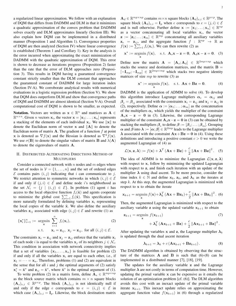
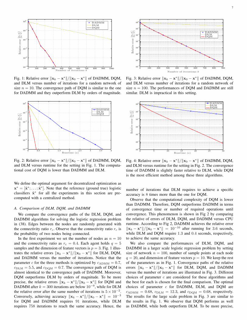
Fig. 1: Relative error ‖xk − x∗‖/‖x0 − x∗‖ of DADMM, DQM,and DLM versus number of iterations for a random network ofsize n = 10. The convergence path of DQM is similar to the onefor DADMM and they outperform DLM by orders of magnitude.

0 0.5 1 1.5 2 2.5 3 3.5 410

−10

10−8

10−6

10−4

10−2

100

Runtime (s)

Relativeerror

‖xk−x∗‖

‖x0−

x∗‖

DADMMDLMDQM

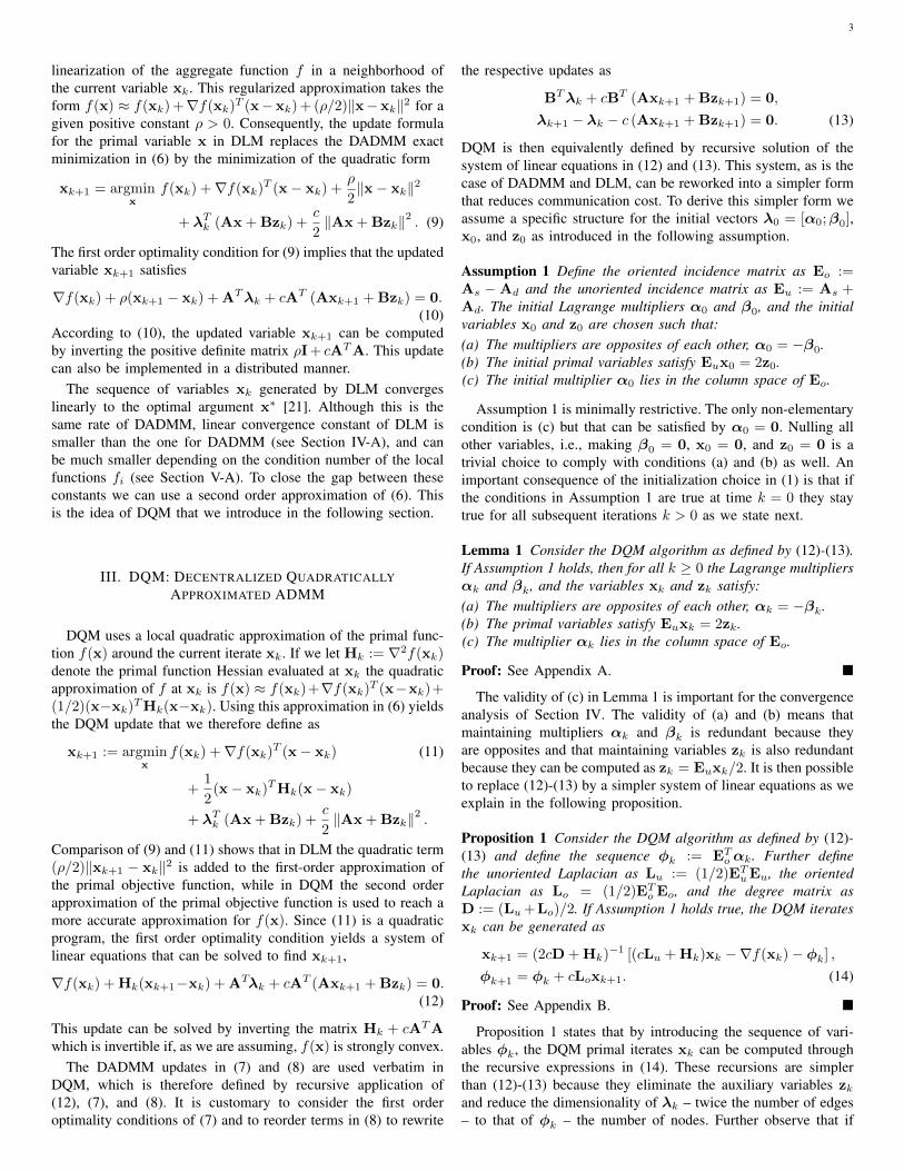
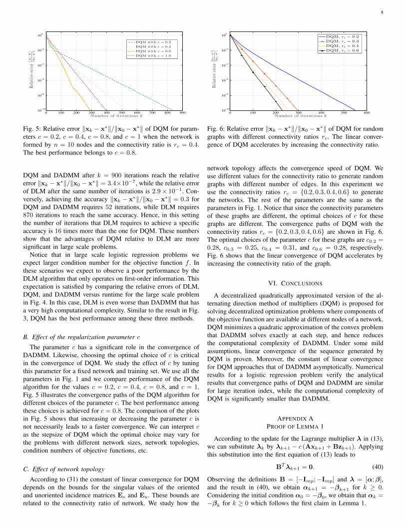
Fig. 2: Relative error ‖xk − x∗‖/‖x0 − x∗‖ of DADMM, DQM,and DLM versus runtime for the setting in Fig. 1. The computa-tional cost of DQM is lower than DADMM and DLM.

We define the optimal argument for decentralized optimization asx∗ = [x∗; . . . ; x∗]. Note that the reference (ground true) logisticclassifiers x∗ for all the experiments in this section are pre-computed with a centralized method.

A. Comparison of DLM, DQM, and DADMM

We compare the convergence paths of the DLM, DQM, andDADMM algorithms for solving the logistic regression problemin (38). Edges between the nodes are randomly generated withthe connectivity ratio rc. Observe that the connectivity ratio rc isthe probability of two nodes being connected.

In the first experiment we set the number of nodes as n = 10and the connectivity ratio as rc = 0.4. Each agent holds q = 5samples and the dimension of feature vectors is p = 3. Fig. 1 illus-trates the relative errors ‖xk − x∗‖/‖x0 − x∗‖ for DLM, DQM,and DADMM versus the number of iterations. Notice that theparameter c for the three methods is optimized by cADMM = 0.7,cDLM = 5.5, and cDQM = 0.7. The convergence path of DQM isalmost identical to the convergence path of DADMM. Moreover,DQM outperforms DLM by orders of magnitude. To be moreprecise, the relative errors ‖xk − x∗‖/‖x0 − x∗‖ for DQM andDADMM after k = 300 iterations are below 10−9, while for DLMthe relative error after the same number of iterations is 5× 10−2.Conversely, achieving accuracy ‖xk − x∗‖/‖x0 − x∗‖ = 10−3

for DQM and DADMM requires 91 iterations, while DLMrequires 758 iterations to reach the same accuracy. Hence, the

0 100 200 300 400 500 600 700 800 90010

−7

10−6

10−5

10−4

10−3

10−2

10−1

100

Number of iterations k

Relativeerror

‖xk−x∗‖

‖x0−x∗‖

DADMMDLMDQM

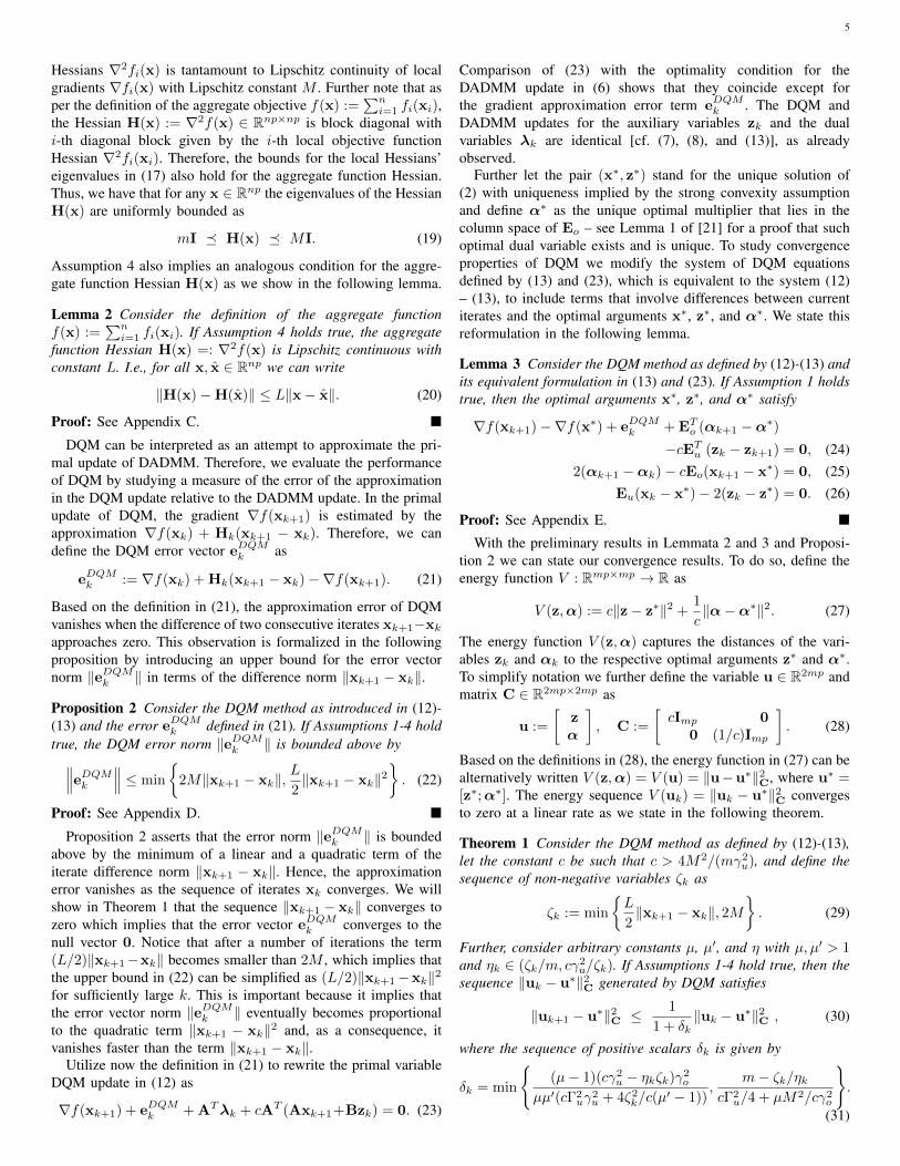
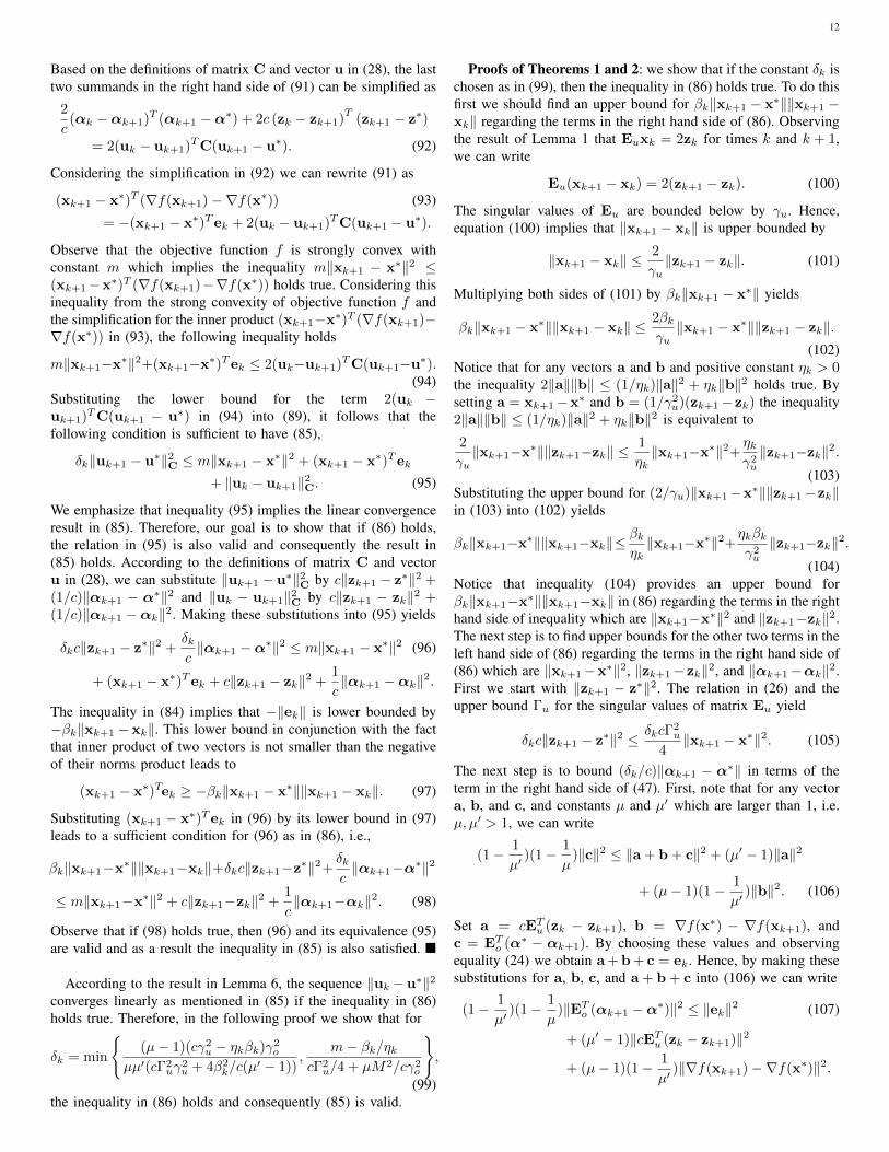
Fig. 3: Relative error ‖xk − x∗‖/‖x0 − x∗‖ of DADMM, DQM,and DLM versus number of iterations for a random network ofsize n = 100. The performances of DQM and DADMM are stillsimilar. DLM is impractical in this setting.

0 5 10 15 20 25 3010

−6

10−5

10−4

10−3

10−2

10−1

100

Runtime (s)

Relativeerror

‖xk−x∗‖

‖x0−

x∗‖

DADMMDLMDQM

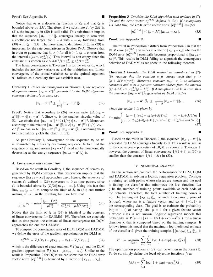
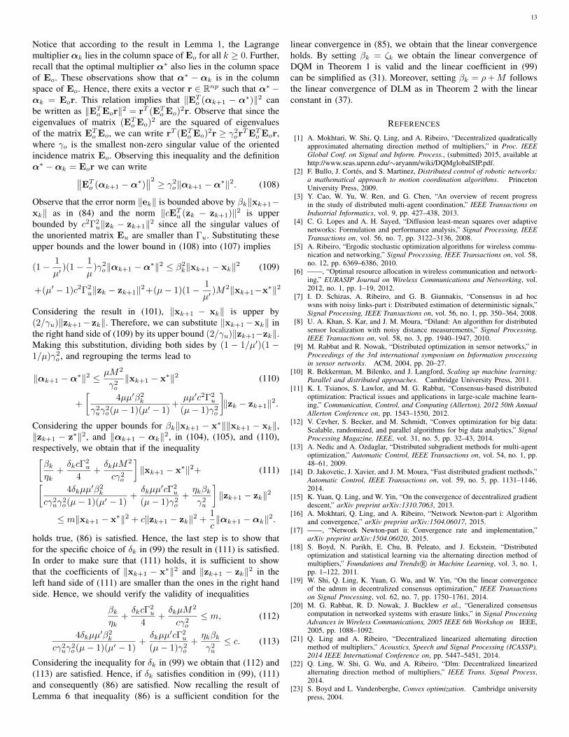
Fig. 4: Relative error ‖xk − x∗‖/‖x0 − x∗‖ of DADMM, DQM,and DLM versus runtime for the setting in Fig. 2. The convergencetime of DADMM is slightly faster relative to DLM, while DQMis the most efficient method among these three algorithms.

number of iterations that DLM requires to achieve a specificaccuracy is 8 times more than the one for DQM.

Observe that the computational complexity of DQM is lowerthan DADMM. Therefore, DQM outperforms DADMM in termsof convergence time or number of required operations untilconvergence. This phenomenon is shown in Fig 2 by comparingthe relative of errors of DLM, DQM, and DADMM versus CPUruntime. According to Fig 2, DADMM achieves the relative error‖xk − x∗‖/‖x0 − x∗‖ = 10−10 after running for 3.6 seconds,while DLM and DQM require 1.3 and 0.4 seconds, respectively,to achieve the same accuracy.

We also compare the performances of DLM, DQM, andDADMM in a larger scale logistic regression problem by settingsize of network n = 100, number of sample points at each nodeq = 20, and dimension of feature vectors p = 10. We keep the restof the parameters as in Fig. 1. Convergence paths of the relativeerrors ‖xk − x∗‖/‖x0 − x∗‖ for DLM, DQM, and DADMMversus the number of iterations are illustrated in Fig. 3. Differentchoices of parameter c are considered for these algorithms andthe best for each is chosen for the final comparison. The optimalchoices of parameter c for DADMM, DLM, and DQM arecADMM = 0.68, cDLM = 12.3, and cDQM = 0.68, respectively.The results for the large scale problem in Fig. 3 are similar tothe results in Fig. 1. We observe that DQM performs as wellas DADMM, while both outperform DLM. To be more precise,

8

0 100 200 300 400 500 600 700 800 90010

−10

10−8

10−6

10−4

10−2

100

Number of iterations k

Relativeerror

‖xk−x∗‖

‖x0−x∗‖

DQM with c = 0.2

DQM with c = 0.4

DQM with c = 0.8

DQM with c = 1.0

Fig. 5: Relative error ‖xk − x∗‖/‖x0 − x∗‖ of DQM for param-eters c = 0.2, c = 0.4, c = 0.8, and c = 1 when the network isformed by n = 10 nodes and the connectivity ratio is rc = 0.4.The best performance belongs to c = 0.8.

DQM and DADMM after k = 900 iterations reach the relativeerror ‖xk − x∗‖/‖x0 − x∗‖ = 3.4×10−7, while the relative errorof DLM after the same number of iterations is 2.9× 10−1. Con-versely, achieving the accuracy ‖xk − x∗‖/‖x0 − x∗‖ = 0.3 forDQM and DADMM requires 52 iterations, while DLM requires870 iterations to reach the same accuracy. Hence, in this settingthe number of iterations that DLM requires to achieve a specificaccuracy is 16 times more than the one for DQM. These numbersshow that the advantages of DQM relative to DLM are moresignificant in large scale problems.

Notice that in large scale logistic regression problems weexpect larger condition number for the objective function f . Inthese scenarios we expect to observe a poor performance by theDLM algorithm that only operates on first-order information. Thisexpectation is satisfied by comparing the relative errors of DLM,DQM, and DADMM versus runtime for the large scale problemin Fig. 4. In this case, DLM is even worse than DADMM that hasa very high computational complexity. Similar to the result in Fig.3, DQM has the best performance among these three methods.

B. Effect of the regularization parameter c

The parameter c has a significant role in the convergence ofDADMM. Likewise, choosing the optimal choice of c is criticalin the convergence of DQM. We study the effect of c by tuningthis parameter for a fixed network and training set. We use all theparameters in Fig. 1 and we compare performance of the DQMalgorithm for the values c = 0.2, c = 0.4, c = 0.8, and c = 1.Fig. 5 illustrates the convergence paths of the DQM algorithm fordifferent choices of the parameter c. The best performance amongthese choices is achieved for c = 0.8. The comparison of the plotsin Fig. 5 shows that increasing or decreasing the parameter c isnot necessarily leads to a faster convergence. We can interpret cas the stepsize of DQM which the optimal choice may vary forthe problems with different network sizes, network topologies,condition numbers of objective functions, etc.

C. Effect of network topology

According to (31) the constant of linear convergence for DQMdepends on the bounds for the singular values of the orientedand unoriented incidence matrices Eo and Eu. These bounds arerelated to the connectivity ratio of network. We study how the

0 100 200 300 400 500 60010

−10

10−8

10−6

10−4

10−2

100

Number of iterations k

Relativeerror

‖xk−x∗‖

‖x0−x∗‖

DQM, rc = 0.2

DQM, rc = 0.3

DQM, rc = 0.4

DQM, rc = 0.6

Fig. 6: Relative error ‖xk − x∗‖/‖x0 − x∗‖ of DQM for randomgraphs with different connectivity ratios rc. The linear conver-gence of DQM accelerates by increasing the connectivity ratio.

network topology affects the convergence speed of DQM. Weuse different values for the connectivity ratio to generate randomgraphs with different number of edges. In this experiment weuse the connectivity ratios rc = {0.2, 0.3, 0.4, 0.6} to generatethe networks. The rest of the parameters are the same as theparameters in Fig. 1. Notice that since the connectivity parametersof these graphs are different, the optimal choices of c for thesegraphs are different. The convergence paths of DQM with theconnectivity ratios rc = {0.2, 0.3, 0.4, 0.6} are shown in Fig. 6.The optimal choices of the parameter c for these graphs are c0.2 =0.28, c0.3 = 0.25, c0.4 = 0.31, and c0.6 = 0.28, respectively.Fig. 6 shows that the linear convergence of DQM accelerates byincreasing the connectivity ratio of the graph.

VI. CONCLUSIONS

A decentralized quadratically approximated version of the al-ternating direction method of multipliers (DQM) is proposed forsolving decentralized optimization problems where components ofthe objective function are available at different nodes of a network.DQM minimizes a quadratic approximation of the convex problemthat DADMM solves exactly at each step, and hence reducesthe computational complexity of DADMM. Under some mildassumptions, linear convergence of the sequence generated byDQM is proven. Moreover, the constant of linear convergencefor DQM approaches that of DADMM asymptotically. Numericalresults for a logistic regression problem verify the analyticalresults that convergence paths of DQM and DADMM are similarfor large iteration index, while the computational complexity ofDQM is significantly smaller than DADMM.

APPENDIX APROOF OF LEMMA 1

According to the update for the Lagrange multiplier λ in (13),we can substitute λk by λk+1 − c (Axk+1 + Bzk+1). Applyingthis substitution into the first equation of (13) leads to

BTλk+1 = 0. (40)

Observing the definitions B = [−Imp;−Imp] and λ = [α;β],and the result in (40), we obtain αk+1 = −βk+1 for k ≥ 0.Considering the initial condition α0 = −β0, we obtain that αk =−βk for k ≥ 0 which follows the first claim in Lemma 1.

9

Based on the definitions A = [As;Ad], B = [−Imp;−Imp],and λ = [α;β], we can split the update for the Lagrangemultiplier λ in (8) as

αk+1 = αk + c[Asxk+1 − zk+1], (41)βk+1 = βk + c[Adxk+1 − zk+1]. (42)

Observing the result that αk = −βk for k ≥ 0, summing up theequations in (41) and (42) yields

(As + Ad)xk+1 = 2zk+1. (43)

Considering the definition of the oriented incidence matrix Eu =As+Ad, we obtain that Euxk = 2zk holds for k > 0. Accordingto the initial condition Eux0 = 2z0, we can conclude that therelation Euxk = 2zk holds for k ≥ 0.

Subtract the update for βk in (42) from the update for αk in(41) and consider the relation βk = −αk to obtain

αk+1 = αk +c

2(As −Ad)xk+1. (44)

Substituting As −Ad in (44) by Eo implies that

αk+1 = αk +c

2Eoxk+1. (45)

Hence, if αk lies in the column space of matrix Eo, then αk+1

also lies in the column space of Eo. According to the thirdcondition of Assumption 1, α0 satisfies this condition, thereforeαk lies in the column space of matrix Eo for all k ≥ 0.

APPENDIX BPROOF OF PROPOSITION 1

The update for the multiplier λ in (8) implies that we cansubstitute λk by λk+1 − c(Axk+1 + Bzk+1) to simplify (12) as

∇f(xk)+Hk(xk+1−xk)+ATλk+1 +cATB (zk − zk+1) = 0.(46)

Considering the first result of Lemma 1 that αk = −βk for k ≥ 0in association with the definition A = [As;Ad] implies that theproduct ATλk+1 is equivalent to

ATλk+1 = ATs αk+1 + AT

d βk+1 = (As −Ad)Tαk+1. (47)

According to the definition Eo := As −Ad, the right hand sideof (47) can be simplified as

ATλk+1 = ETo αk+1. (48)

Based on the structures of the matrices A and B, and thedefinition Eu := As + Ad, we can simplify ATB as

ATB = −ATs −AT

d = −ETu . (49)

Substituting the results in (48) and (49) into (46) leads to

∇f(xk) + Hk(xk+1 − xk) + ETo αk+1 + cET

u (zk+1 − zk) = 0.(50)

The second result in Lemma 1 states that zk = Euxk/2.Multiplying both sides of this equality by ET

u from left we obtainthat ET

u zk = ETuEuxk/2 for k ≥ 0. Observing the definition

of the unoriented Laplacian Lu := ETuEu/2, we obtain that the

product ETu zk is equal to Luxk for k ≥ 0. Therefore, in (50) we

can substitute ETu (zk+1 − zk) by Lu(xk+1 − xk) and write

∇f(xk) + (Hk + cLu) (xk+1 − xk) + ETo αk+1 = 0. (51)

Observe that the new variables φk are defined as φk := ETo αk.

Multiplying both sides of (45) by ETo from the left hand side and

considering the definition of oriented Laplacian Lo = ETo Eo/2

follows the update rule of φk in (14), i.e.,

φk+1 = φk + cLoxk+1. (52)

According to the definition φk = ETo αk and the update formula

in (52), we can conclude that ETo αk+1 = φk+1 = φk+cLoxk+1.

Substituting ETo αk+1 by φk + cLoxk+1 in (51) yields

∇f(xk) + (Hk + cLu) (xk+1−xk) +φk + cLoxk+1 = 0. (53)

Observing the definition D = (Lu + Lo)/2 we rewrite (53) as

(Hk + 2cD)xk+1 = (Hk + cLu)xk −∇f(xk)− φk. (54)

Multiplying both sides of (54) by (Hk + 2cD)−1 from the left

hand side yields the first update in (14).

APPENDIX CPROOF OF LEMMA 2

Consider two arbitrary vectors x := [x1; . . . ;xn] ∈ Rnp

and x := [x1; . . . ; xn] ∈ Rnp. Since the aggregate functionHessian is block diagonal where the i-th diagonal block isgiven by ∇2fi(xi), we obtain that the difference of HessiansH(x)−H(x) is also block diagonal where the i-th diagonal blockH(x)ii −H(x)ii is

H(x)ii −H(x)ii = ∇2fi(xi)−∇2fi(xi). (55)

Consider any vector v ∈ Rnp and separate each p componentsof vector v and consider it as a new vector called vi ∈ Rp,i.e., v := [v1; . . . ;vn]. Observing the relation for the differenceH(x) − H(x) in (55), the symmetry of matrices H(x) andH(x), and the definition of Euclidean norm of a matrix that‖A‖ =

√λmax(ATA), we obtain that the squared difference

norm ‖H(x)−H(x)‖2 can be written as

‖H(x)−H(x)‖2 = maxv

vT [H(x)−H(x)]2v

‖v‖2(56)

= maxv

∑ni=1 v

Ti

[∇2fi(xi)−∇2fi(xi)

]2vi

‖v‖2

Using the Cauchy-Schwarz inequality we can write

vTi

[∇2fi(xi)−∇2fi(xi)

]2vi ≤

∥∥∇2fi(xi)−∇2fi(xi)∥∥2‖vi‖2

(57)Substituting the upper bound in (57) into (56) implies that thesquared norm ‖H(x)−H(x)‖2 is bounded above as

‖H(x)−H(x)‖2 ≤ maxv

∑ni=1

∥∥∇2fi(xi)−∇2fi(xi)∥∥2 ‖vi‖2

‖v‖2.

(58)Observe that Assumption 3 states that local objective functionsHessian ∇2fi(xi) are Lipschitz continuous with constant L, i.e.‖∇2fi(xi)−∇2fi(xi)‖ ≤ L‖xi−xi‖. Considering this inequalitythe upper bound in (58) can be changed by replacing ‖∇2fi(xi)−∇2fi(xi)‖ by L‖xi − xi‖ which yields

‖H(x)−H(x)‖2 ≤ maxv

L2∑n

i=1 ‖xi − xi‖2 ‖vi‖2∑ni=1 ‖vi‖2

. (59)

Note that for any sequences of scalars such as ai and bi, theinequality

∑ni=1 a

2i b

2i ≤ (

∑ni=1 a

2i )(∑n

i=1 b2i ) holds. If we divide

10

both sides of this relation by∑n

i=1 b2i and set ai = ‖xi− xi‖ and

bi = ‖vi‖, we obtain∑ni=1 ‖xi − xi‖2 ‖vi‖2∑n

i=1 ‖vi‖2≤

n∑i=1

‖xi − xi‖2 . (60)

Combining the two inequalities in (59) and (60) leads to

‖H(x)−H(x)‖2 ≤ maxv

L2n∑

i=1

‖xi − xi‖2 . (61)

Since the right hand side of (61) does not depend on v wecan eliminate the maximization with respect to v. Further, notethat according to the structure of vectors x and x, we canwrite ‖x− x‖2 =

∑ni=1 ‖xi − xi‖2. These two observations in

association with (61) imply that

‖H(x)−H(x)‖2 ≤ L2 ‖x− x‖2 , (62)

Computing the square roots of terms in (62) yields (20).

APPENDIX DPROOFS OF PROPOSITIONS 2 AND 3

The fundamental theorem of calculus implies that the differenceof gradients ∇f(xk+1)−∇f(xk) can be written as

∇f(xk+1)−∇f(xk) =

∫ 1

0

H(sxk+1+(1−s)xk)(xk+1−xk) ds.

(63)By computing norms of both sides of (63) and considering thatnorm of integral is smaller than integral of norm we obtain that

‖∇f(xk+1)−∇f(xk)‖≤∫ 1

0

‖H(sxk+1+(1−s)xk)(xk+1−xk)‖ds.(64)

The upper bound M for the eigenvalues of the Hessians as in(19), implies that ‖H (sx + (1− s)x) (x − x)‖ ≤ M‖x − x‖.Substituting this upper bound into (64) leads to

‖∇f(xk+1)−∇f(xk)‖ ≤M‖xk+1 − xk‖. (65)

The error vector norm ‖eDLMk ‖ in (34) is bounded above as

‖eDLMk ‖ ≤ ‖∇f(xk+1)−∇f(xk)‖+ ρ‖xk+1 − xk‖. (66)

By substituting the upper bound for ‖∇f(xk+1) − ∇f(xk)‖ in(65) into (66), the claim in (35) follows.

To prove (22), first we show that ‖eDQMk ‖ ≤ 2M‖xk+1−xk‖

holds. Observe that the norm of error vector eDQMk defined (21)

can be upper bounded using the triangle inequality as

‖eDQMk ‖ ≤ ‖∇f(xk+1)−∇f(xk)‖+ ‖Hk(xk+1 − xk)‖. (67)

Based on the Cauchy-Schwarz inequality and the upper bound Mfor the eigenvalues of Hessians as in (19), we obtain ‖Hk(xk+1−xk)‖ ≤ M‖xk+1 − xk‖. Further, as mentioned in (65) thedifference of gradients ‖∇f(xk+1)−∇f(xk)‖ is upper boundedby M‖xk+1−xk‖. Substituting these upper bounds for the termsin the right hand side of (67) yields

‖eDQMk ‖ ≤ 2M‖xk+1 − xk‖. (68)

The next step is to show that ‖eDQMk ‖ ≤ (L/2)‖xk+1 − xk‖2.

Adding and subtracting the integral∫ 1

0H(xk)(xk+1 − xk) ds to

the right hand side of (63) results in

∇f(xk+1)−∇f(xk) =

∫ 1

0

H(xk)(xk+1 − xk) ds

+

∫ 1

0

[H(sxk+1 + (1− s)xk)−H(xk)] (xk+1 − xk) ds. (69)

First observe that the integral∫ 1

0H(xk)(xk+1 − xk) ds can be

simplified as H(xk)(xk+1 − xk). Observing this simplificationand regrouping the terms yield

∇f(xk+1)−∇f(xk)−H(xk)(xk+1 − xk) =∫ 1

0

[H(sxk+1 + (1− s)xk)−H(xk)] (xk+1 − xk) ds. (70)

Computing norms of both sides of (70), considering the factthat norm of integral is smaller than integral of norm, and usingCauchy-Schwarz inequality lead to

‖∇f(xk+1)−∇f(xk)−H(xk)(xk+1 − xk)‖ ≤ (71)∫ 1

0

‖H(sxk+1 + (1− s)xk)−H(xk)‖ ‖xk+1 − xk‖ds.

Lipschitz continuity of the Hessian as in (20) implies that‖H(sxk+1 + (1− s)xk)−H(xk)‖ ≤ sL‖xk+1 − xk‖. By sub-stituting this upper bound into the integral in (71) and substitutingthe left hand side of (71) by ‖eDQM

k ‖ we obtain

‖eDQMk ‖ ≤

∫ 1

0

sL‖xk+1 − xk‖2ds. (72)

Simplification of the integral in (72) follows

‖eDQMk ‖ ≤ L

2‖xk+1 − xk‖2. (73)

The results in (68) and (73) follow the claim in (22).

APPENDIX EPROOF OF LEMMA 3

In this section we first introduce an equivalent version ofLemma 3 for the DLM algorithm. Then, we show the validityof both lemmata in a general proof.

Lemma 4 Consider DLM as defined by (7)-(9). If Assumption 1holds true, then the optimal arguments x∗, z∗, and α∗ satisfy

∇f(xk+1)−∇f(x∗) + eDLMk + ET

o (αk+1 −α∗)

−cETu (zk − zk+1) = 0, (74)

2(αk+1 −αk)− cEo(xk+1 − x∗) = 0, (75)Eu(xk − x∗)− 2(zk − z∗) = 0. (76)

Notice that the claims in Lemmata 3 and 4 are identical exceptin the error term of the first equalities. To provide a generalframework to prove the claim in these lemmata we introduce ekas the general error vector. By replacing ek with eDQM

k we obtainthe result of DQM in Lemma 3 and by setting ek = eDLM

k theresult in Lemma 4 follows. We start with the following Lemmathat captures the KKT conditions of optimization problem (4).

Lemma 5 Consider the optimization problem (4). The optimalLagrange multiplier α∗, primal variable x∗ and auxiliary variablez∗ satisfy the following system of equations

∇f(x∗) + ETo α∗ = 0, Eox

∗ = 0, Eux∗ = 2z∗. (77)

11

Proof: First observe that the KKT conditions of the decentralizedoptimization problem in (4) are given by

∇f(x∗) + ATλ∗ = 0, BTλ∗ = 0, Ax∗ + Bz∗ = 0. (78)

Based on the definitions of the matrix B = [−Imp;−Imp] andthe optimal Lagrange multiplier λ∗ := [α∗;β∗], we obtain thatBTλ∗ = 0 in (78) is equivalent to α∗ = −β∗. Considering thisresult and the definition A = [As;Ad], we obtain

ATλ∗ = ATs α∗ + AT

d β∗ = (As −Ad)Tα∗. (79)

The definition Eo := As−Ad implies that the right hand side of(79) can be simplified as ET

o α∗ which shows ATλ∗ = ET

o α∗.

Substituting ATλ∗ by ETo α∗ into the first equality in (78) follows

the first claim in (77).Decompose the KKT condition Ax∗ +Bz∗ = 0 in (78) based

on the definitions of A and B as

Asx∗ − z = 0, Adx

∗ − z = 0. (80)

Subtracting the equalities in (80) implies that (As −Ad)x∗ = 0which by considering the definition Eo = As −Ad, the secondequation in (77) follows. Summing up the equalities in (80) yields(As + Ad)x∗ = 2z. This observation in association with thedefinition Eu = As −Ad follows the third equation in (77). �

Proofs of Lemmata 3 and 4: First note that the results inLemma 1 are also valid for DLM [22]. Now, consider the firstorder optimality condition for primal updates of DQM and DLMin (12) and (10), respectively. Further, recall the definitions oferror vectors eDQM

k and eDLMk in (21) and (34), respectively.

Combining these observations we obtain that

∇f(xk+1) + ek + ATλk + cAT (Axk+1 + Bzk) = 0. (81)

Notice that by setting ek = eDQMk we obtain the update for

primal variable of DQM; likewise, setting ek = eDLMk yields to

the update of DLM.Observe that the relation λk = λk+1 − c(Axk+1 + Bzk+1)

holds for both DLM and DQM according to to the update formulafor Lagrange multiplier in (8) and (13). Substituting λk by λk+1−c(Axk+1 + Bzk+1) in (81) follows

∇f(xk+1) + ek + ATλk+1 + cATB (zk − zk+1) = 0 (82)

Based on the result in Lemma 1, the components of the Lagrangemultiplier λ = [α;β] satisfy αk+1 = −βk+1. Hence, the productATλk+1 can be simplified as AT

s αk+1 −ATd αk+1 = ET

o αk+1

considering the definition that Eo = As−Ad. Furthermore, notethat according to the definitions we have that A = [As;Ad] andB = [−I;−I] which implies that ATB = −(As+Ad)T = −ET

u .By making these substitutions into (82) we can write

∇f(xk+1) + ek + ETo αk+1 − cET

u (zk − zk+1) = 0. (83)

The first result in Lemma 5 is equivalent to ∇f(x∗)+ETo α∗ = 0.

Subtracting both sides of this equation from the relation in (83)follows the first claim of Lemmata 3 and 4.

We proceed to prove the second and third claims in Lemmata 3and 4. The update formula for αk in (45) and the second result inLemma 5 that Eox

∗ = 0 imply that the second claim of Lemmata3 and 4 are valid. Further, the result in Lemma 1 guaranteaes thatEuxk = 2zk. This result in conjunction with the result in Lemma5 that Eux

∗ = 2z∗ leads to the third claim of Lemmata 3 and 4.

APPENDIX FPROOFS OF THEOREMS 1 AND 2

To prove Theorems 1 and 2 we show a sufficient conditionfor the claims in these theorems. Then, we prove these theoremsby showing validity of the sufficient condition. To do so, we usethe general coefficient βk which is equivalent to ζk in the DQMalgorithm and equivalent to ρ + M in the DLM method. Thesedefinitions and the results in Propositions 2 and 3 imply that

‖ek‖ ≤ βk‖xk+1 − xk‖, (84)

where ek is eDQMk in DQM and eDLM

k in DLM. The sufficientcondition of Theorems 1 and 2 is studied in the following lemma.

Lemma 6 Consider the DLM and DQM algorithms as definedin (7)-(9) and (12)-(13), respectively. Further, conducer δk as asequence of positive scalars. If Assumptions 1-4 hold true thenthe sequence ‖uk − u∗‖2C converges linearly as

‖uk+1 − u∗‖2C ≤1

1 + δk‖uk − u∗‖2C, (85)

if the following inequality holds true,

βk‖xk+1−x∗‖‖xk+1−xk‖+δkc‖zk+1−z∗‖2+δkc‖αk+1−α∗‖2

≤ m‖xk+1−x∗‖2 + c‖zk+1−zk‖2 +1

c‖αk+1−αk‖2. (86)

Proof: Proving linear convergence of the sequence ‖uk − u∗‖2Cas mentioned in (85) is equivalent to showing that

δk‖uk+1 − u∗‖2C ≤ ‖uk − u∗‖2C − ‖uk+1 − u∗‖2C. (87)

According to the definition ‖a‖2C := aTCa we can show that

2(uk − uk+1)TC(uk+1 − u∗) = ‖uk − u∗‖2C − ‖uk+1 − u∗‖2C− ‖uk − uk+1‖2C. (88)

The relation in (88) shows that the right hand side of (87) can besubstituted by 2(uk − uk+1)TC(uk+1 − u∗) + ‖uk − uk+1‖2C.Applying this substitution into (87) leads to

δk‖uk+1−u∗‖2C ≤ 2(uk−uk+1)TC(uk+1−u∗)+‖uk−uk+1‖2C(89)

This observation implies that to prove the linear convergence asclaimed in (85), the inequality in (89) should be satisfied.

We proceed by finding a lower bound for the term 2(uk −uk+1)TC(uk+1 − u∗) in (89). By regrouping the terms in (83)and multiplying both sides of equality by (xk+1 − x∗)T fromthe left hand side we obtain that the inner product (xk+1 −x∗)T (∇f(xk+1)−∇f(x∗)) is equivalent to

(xk+1 − x∗)T (∇f(xk+1)−∇f(x∗)) =

− (xk+1 − x∗)Tek − (xk+1 − x∗)TETo (αk+1 −α∗)

+ c(xk+1 − x∗)TETu (zk − zk+1). (90)

Based on (25), we can substitute (xk+1 − x∗)TETo (αk+1 − α∗)

in (90) by (2/c)(αk+1 − αk)T (αk+1 − α∗). Further, the resultin (26) implies that the term c(xk+1 − x∗)TET

u (zk − zk+1) in(90) is equivalent to 2c (zk − zk+1)

T(zk+1−z∗). Applying these

substitutions into (90) leads to

(xk+1−x∗)T (∇f(xk+1)−∇f(x∗)) = −(xk+1−x∗)Tek (91)

+2

c(αk −αk+1)T (αk+1 −α∗)+2c (zk − zk+1)

T(zk+1 − z∗).

12

Based on the definitions of matrix C and vector u in (28), the lasttwo summands in the right hand side of (91) can be simplified as

2

c(αk −αk+1)T (αk+1 −α∗) + 2c (zk − zk+1)

T(zk+1 − z∗)

= 2(uk − uk+1)TC(uk+1 − u∗). (92)

Considering the simplification in (92) we can rewrite (91) as

(xk+1 − x∗)T (∇f(xk+1)−∇f(x∗)) (93)

= −(xk+1 − x∗)Tek + 2(uk − uk+1)TC(uk+1 − u∗).

Observe that the objective function f is strongly convex withconstant m which implies the inequality m‖xk+1 − x∗‖2 ≤(xk+1−x∗)T (∇f(xk+1)−∇f(x∗)) holds true. Considering thisinequality from the strong convexity of objective function f andthe simplification for the inner product (xk+1−x∗)T (∇f(xk+1)−∇f(x∗)) in (93), the following inequality holds

m‖xk+1−x∗‖2+(xk+1−x∗)Tek ≤ 2(uk−uk+1)TC(uk+1−u∗).(94)

Substituting the lower bound for the term 2(uk −uk+1)TC(uk+1 − u∗) in (94) into (89), it follows that thefollowing condition is sufficient to have (85),

δk‖uk+1 − u∗‖2C ≤ m‖xk+1 − x∗‖2 + (xk+1 − x∗)Tek

+ ‖uk − uk+1‖2C. (95)

We emphasize that inequality (95) implies the linear convergenceresult in (85). Therefore, our goal is to show that if (86) holds,the relation in (95) is also valid and consequently the result in(85) holds. According to the definitions of matrix C and vectoru in (28), we can substitute ‖uk+1 − u∗‖2C by c‖zk+1 − z∗‖2 +(1/c)‖αk+1 − α∗‖2 and ‖uk − uk+1‖2C by c‖zk+1 − zk‖2 +(1/c)‖αk+1 −αk‖2. Making these substitutions into (95) yields

δkc‖zk+1 − z∗‖2 +δkc‖αk+1 −α∗‖2 ≤ m‖xk+1 − x∗‖2 (96)

+ (xk+1 − x∗)Tek + c‖zk+1 − zk‖2 +1

c‖αk+1 −αk‖2.

The inequality in (84) implies that −‖ek‖ is lower bounded by−βk‖xk+1 − xk‖. This lower bound in conjunction with the factthat inner product of two vectors is not smaller than the negativeof their norms product leads to

(xk+1 − x∗)Tek ≥ −βk‖xk+1 − x∗‖‖xk+1 − xk‖. (97)

Substituting (xk+1 − x∗)Tek in (96) by its lower bound in (97)leads to a sufficient condition for (96) as in (86), i.e.,

βk‖xk+1−x∗‖‖xk+1−xk‖+δkc‖zk+1−z∗‖2+δkc‖αk+1−α∗‖2

≤ m‖xk+1−x∗‖2 + c‖zk+1−zk‖2 +1

c‖αk+1−αk‖2. (98)

Observe that if (98) holds true, then (96) and its equivalence (95)are valid and as a result the inequality in (85) is also satisfied. �

According to the result in Lemma 6, the sequence ‖uk −u∗‖2converges linearly as mentioned in (85) if the inequality in (86)holds true. Therefore, in the following proof we show that for

δk = min

{(µ− 1)(cγ2u − ηkβk)γ2o

µµ′(cΓ2uγ

2u + 4β2

k/c(µ′ − 1))

,m− βk/ηk

cΓ2u/4 + µM2/cγ2o

},

(99)the inequality in (86) holds and consequently (85) is valid.

Proofs of Theorems 1 and 2: we show that if the constant δk ischosen as in (99), then the inequality in (86) holds true. To do thisfirst we should find an upper bound for βk‖xk+1 − x∗‖‖xk+1 −xk‖ regarding the terms in the right hand side of (86). Observingthe result of Lemma 1 that Euxk = 2zk for times k and k + 1,we can write

Eu(xk+1 − xk) = 2(zk+1 − zk). (100)

The singular values of Eu are bounded below by γu. Hence,equation (100) implies that ‖xk+1 − xk‖ is upper bounded by

‖xk+1 − xk‖ ≤2

γu‖zk+1 − zk‖. (101)

Multiplying both sides of (101) by βk‖xk+1 − x∗‖ yields

βk‖xk+1 − x∗‖‖xk+1 − xk‖ ≤2βkγu‖xk+1 − x∗‖‖zk+1 − zk‖.

(102)Notice that for any vectors a and b and positive constant ηk > 0the inequality 2‖a‖‖b‖ ≤ (1/ηk)‖a‖2 + ηk‖b‖2 holds true. Bysetting a = xk+1−x∗ and b = (1/γ2u)(zk+1−zk) the inequality2‖a‖‖b‖ ≤ (1/ηk)‖a‖2 + ηk‖b‖2 is equivalent to

2

γu‖xk+1−x∗‖‖zk+1−zk‖ ≤

1

ηk‖xk+1−x∗‖2+

ηkγ2u‖zk+1−zk‖2.

(103)Substituting the upper bound for (2/γu)‖xk+1−x∗‖‖zk+1−zk‖in (103) into (102) yields

βk‖xk+1−x∗‖‖xk+1−xk‖≤βkηk‖xk+1−x∗‖2+

ηkβkγ2u‖zk+1−zk‖2.

(104)Notice that inequality (104) provides an upper bound forβk‖xk+1−x∗‖‖xk+1−xk‖ in (86) regarding the terms in the righthand side of inequality which are ‖xk+1−x∗‖2 and ‖zk+1−zk‖2.The next step is to find upper bounds for the other two terms in theleft hand side of (86) regarding the terms in the right hand side of(86) which are ‖xk+1−x∗‖2, ‖zk+1−zk‖2, and ‖αk+1−αk‖2.First we start with ‖zk+1 − z∗‖2. The relation in (26) and theupper bound Γu for the singular values of matrix Eu yield

δkc‖zk+1 − z∗‖2 ≤ δkcΓ2u

4‖xk+1 − x∗‖2. (105)

The next step is to bound (δk/c)‖αk+1 − α∗‖ in terms of theterm in the right hand side of (47). First, note that for any vectora, b, and c, and constants µ and µ′ which are larger than 1, i.e.µ, µ′ > 1, we can write

(1− 1

µ′)(1− 1

µ)‖c‖2 ≤ ‖a + b + c‖2 + (µ′ − 1)‖a‖2

+ (µ− 1)(1− 1

µ′)‖b‖2. (106)

Set a = cETu (zk − zk+1), b = ∇f(x∗) − ∇f(xk+1), and

c = ETo (α∗ − αk+1). By choosing these values and observing

equality (24) we obtain a+b+ c = ek. Hence, by making thesesubstitutions for a, b, c, and a + b + c into (106) we can write

(1− 1

µ′)(1− 1

µ)‖ET

o (αk+1 −α∗)‖2 ≤ ‖ek‖2 (107)

+ (µ′ − 1)‖cETu (zk − zk+1)‖2

+ (µ− 1)(1− 1

µ′)‖∇f(xk+1)−∇f(x∗)‖2.

13

Notice that according to the result in Lemma 1, the Lagrangemultiplier αk lies in the column space of Eo for all k ≥ 0. Further,recall that the optimal multiplier α∗ also lies in the column spaceof Eo. These observations show that α∗ − αk is in the columnspace of Eo. Hence, there exits a vector r ∈ Rnp such that α∗ −αk = Eor. This relation implies that ‖ET

o (αk+1 − α∗)‖2 canbe written as ‖ET

o Eor‖2 = rT (ETo Eo)2r. Observe that since the

eigenvalues of matrix (ETo Eo)2 are the squared of eigenvalues

of the matrix ETo Eo, we can write rT (ET

o Eo)2r ≥ γ2orTETo Eor,

where γo is the smallest non-zero singular value of the orientedincidence matrix Eo. Observing this inequality and the definitionα∗ −αk = Eor we can write∥∥ET

o (αk+1 −α∗)∥∥2 ≥ γ2o‖αk+1 −α∗‖2. (108)

Observe that the error norm ‖ek‖ is bounded above by βk‖xk+1−xk‖ as in (84) and the norm ‖cET

u (zk − zk+1)‖2 is upperbounded by c2Γ2

u‖zk − zk+1‖2 since all the singular values ofthe unoriented matrix Eu are smaller than Γu. Substituting theseupper bounds and the lower bound in (108) into (107) implies

(1− 1

µ′)(1− 1

µ)γ2o‖αk+1 −α∗‖2 ≤ β2

k‖xk+1 − xk‖2 (109)

+(µ′ − 1)c2Γ2u‖zk − zk+1‖2+(µ− 1)(1− 1

µ′)M2‖xk+1−x∗‖2

Considering the result in (101), ‖xk+1 − xk‖ is upper by(2/γu)‖zk+1−zk‖. Therefore, we can substitute ‖xk+1−xk‖ inthe right hand side of (109) by its upper bound (2/γu)‖zk+1−zk‖.Making this substitution, dividing both sides by (1 − 1/µ′)(1 −1/µ)γ2o , and regrouping the terms lead to

‖αk+1 −α∗‖2 ≤ µM2

γ2o‖xk+1 − x∗‖2 (110)

+

[4µµ′β2

k

γ2uγ2o(µ− 1)(µ′ − 1)

+µµ′c2Γ2

u

(µ− 1)γ2o

]‖zk − zk+1‖2.

Considering the upper bounds for βk‖xk+1 − x∗‖‖xk+1 − xk‖,‖zk+1 − z∗‖2, and ‖αk+1 − αk‖2, in (104), (105), and (110),respectively, we obtain that if the inequality[βkηk

+δkcΓ

2u

4+δkµM

2

cγ2o

]‖xk+1 − x∗‖2+ (111)[

4δkµµ′β2

k

cγ2uγ2o(µ− 1)(µ′ − 1)

+δkµµ

′cΓ2u

(µ− 1)γ2o+ηkβkγ2u

]‖zk+1 − zk‖2

≤ m‖xk+1 − x∗‖2 + c‖zk+1 − zk‖2 +1

c‖αk+1 −αk‖2.

holds true, (86) is satisfied. Hence, the last step is to show thatfor the specific choice of δk in (99) the result in (111) is satisfied.In order to make sure that (111) holds, it is sufficient to showthat the coefficients of ‖xk+1 − x∗‖2 and ‖zk+1 − zk‖2 in theleft hand side of (111) are smaller than the ones in the right handside. Hence, we should verify the validity of inequalities

βkηk

+δkcΓ

2u

4+δkµM

2

cγ2o≤ m, (112)

4δkµµ′β2

k

cγ2uγ2o(µ− 1)(µ′ − 1)

+δkµµ

′cΓ2u

(µ− 1)γ2o+ηkβkγ2u≤ c. (113)

Considering the inequality for δk in (99) we obtain that (112) and(113) are satisfied. Hence, if δk satisfies condition in (99), (111)and consequently (86) are satisfied. Now recalling the result ofLemma 6 that inequality (86) is a sufficient condition for the

linear convergence in (85), we obtain that the linear convergenceholds. By setting βk = ζk we obtain the linear convergence ofDQM in Theorem 1 is valid and the linear coefficient in (99)can be simplified as (31). Moreover, setting βk = ρ+M followsthe linear convergence of DLM as in Theorem 2 with the linearconstant in (37).

REFERENCES

[1] A. Mokhtari, W. Shi, Q. Ling, and A. Ribeiro, “Decentralized quadraticallyapproximated alternating direction method of multipliers,” in Proc. IEEEGlobal Conf. on Signal and Inform. Process., (submitted) 2015, available athttp://www.seas.upenn.edu/∼aryanm/wiki/DQMglobalSIP.pdf.

[2] F. Bullo, J. Cortes, and S. Martinez, Distributed control of robotic networks:a mathematical approach to motion coordination algorithms. PrincetonUniversity Press, 2009.

[3] Y. Cao, W. Yu, W. Ren, and G. Chen, “An overview of recent progressin the study of distributed multi-agent coordination,” IEEE Transactions onIndustrial Informatics, vol. 9, pp. 427–438, 2013.

[4] C. G. Lopes and A. H. Sayed, “Diffusion least-mean squares over adaptivenetworks: Formulation and performance analysis,” Signal Processing, IEEETransactions on, vol. 56, no. 7, pp. 3122–3136, 2008.

[5] A. Ribeiro, “Ergodic stochastic optimization algorithms for wireless commu-nication and networking,” Signal Processing, IEEE Transactions on, vol. 58,no. 12, pp. 6369–6386, 2010.

[6] ——, “Optimal resource allocation in wireless communication and network-ing,” EURASIP Journal on Wireless Communications and Networking, vol.2012, no. 1, pp. 1–19, 2012.

[7] I. D. Schizas, A. Ribeiro, and G. B. Giannakis, “Consensus in ad hocwsns with noisy links-part i: Distributed estimation of deterministic signals,”Signal Processing, IEEE Transactions on, vol. 56, no. 1, pp. 350–364, 2008.

[8] U. A. Khan, S. Kar, and J. M. Moura, “Diland: An algorithm for distributedsensor localization with noisy distance measurements,” Signal Processing,IEEE Transactions on, vol. 58, no. 3, pp. 1940–1947, 2010.

[9] M. Rabbat and R. Nowak, “Distributed optimization in sensor networks,” inProceedings of the 3rd international symposium on Information processingin sensor networks. ACM, 2004, pp. 20–27.

[10] R. Bekkerman, M. Bilenko, and J. Langford, Scaling up machine learning:Parallel and distributed approaches. Cambridge University Press, 2011.

[11] K. I. Tsianos, S. Lawlor, and M. G. Rabbat, “Consensus-based distributedoptimization: Practical issues and applications in large-scale machine learn-ing,” Communication, Control, and Computing (Allerton), 2012 50th AnnualAllerton Conference on, pp. 1543–1550, 2012.

[12] V. Cevher, S. Becker, and M. Schmidt, “Convex optimization for big data:Scalable, randomized, and parallel algorithms for big data analytics,” SignalProcessing Magazine, IEEE, vol. 31, no. 5, pp. 32–43, 2014.

[13] A. Nedic and A. Ozdaglar, “Distributed subgradient methods for multi-agentoptimization,” Automatic Control, IEEE Transactions on, vol. 54, no. 1, pp.48–61, 2009.

[14] D. Jakovetic, J. Xavier, and J. M. Moura, “Fast distributed gradient methods,”Automatic Control, IEEE Transactions on, vol. 59, no. 5, pp. 1131–1146,2014.

[15] K. Yuan, Q. Ling, and W. Yin, “On the convergence of decentralized gradientdescent,” arXiv preprint arXiv:1310.7063, 2013.

[16] A. Mokhtari, Q. Ling, and A. Ribeiro, “Network Newton-part i: Algorithmand convergence,” arXiv preprint arXiv:1504.06017, 2015.

[17] ——, “Network Newton-part ii: Convergence rate and implementation,”arXiv preprint arXiv:1504.06020, 2015.

[18] S. Boyd, N. Parikh, E. Chu, B. Peleato, and J. Eckstein, “Distributedoptimization and statistical learning via the alternating direction method ofmultipliers,” Foundations and Trends R© in Machine Learning, vol. 3, no. 1,pp. 1–122, 2011.

[19] W. Shi, Q. Ling, K. Yuan, G. Wu, and W. Yin, “On the linear convergenceof the admm in decentralized consensus optimization,” IEEE Transactionson Signal Processing, vol. 62, no. 7, pp. 1750–1761, 2014.

[20] M. G. Rabbat, R. D. Nowak, J. Bucklew et al., “Generalized consensuscomputation in networked systems with erasure links,” in Signal ProcessingAdvances in Wireless Communications, 2005 IEEE 6th Workshop on IEEE,2005, pp. 1088–1092.

[21] Q. Ling and A. Ribeiro, “Decentralized linearized alternating directionmethod of multipliers,” Acoustics, Speech and Signal Processing (ICASSP),2014 IEEE International Conference on, pp. 5447–5451, 2014.

[22] Q. Ling, W. Shi, G. Wu, and A. Ribeiro, “Dlm: Decentralized linearizedalternating direction method of multipliers,” IEEE Trans. Signal Process,2014.

[23] S. Boyd and L. Vandenberghe, Convex optimization. Cambridge universitypress, 2004.