1

Abstract—Screen content sequences are ubiquitous type of video data in numerous multimedia applications like video conferencing, remote education, and cloud gaming. These sequences are characterized for depicting a mix of computer generated graphics, text, and camera-captured material. Such a mix poses several challenges, as the content usually depicts multiple strong discontinuities, which are hard to encode using current techniques. Differential Pulse Code Modulation (DPCM)-based intra-prediction has shown to improve coding efficiency for these sequences. In this paper we propose Sample-based Edge and Angular Prediction (SEAP), a collection of DPCM-based intra-prediction modes to improve lossless coding of screen content. SEAP is aimed at accurately predicting regions depicting not only camera-captured material, but also those depicting strong edges. It incorporates modes that allow selecting the best predictor for each pixel individually based on the characteristics of the causal neighborhood of the target pixel. We incorporate SEAP into HEVC intra-prediction. Evaluation results on various screen content sequences show the advantages of SEAP over other DPCM-based approaches, with bit-rate reductions of up to 19.56% compared to the standardized RDPCM method. When used in conjunction with the coding tools of the Screen Content Coding Extensions, SEAP provides bit-rate reductions of up to 8.63% compared to RDPCM.

Index Terms— HEVC intra-prediction, lossless coding, DPCM, edge prediction, screen content.

I. INTRODUCTION HE High Efficiency Video Coding (HEVC) standard is proposed by the Joint Collaborative Team on Video

Coding (JCT-VC), which is jointly established by the ITU-T Video Coding Experts Group (VCEG) and the ISO/IEC Moving Picture Expert Group (MPEG) [1]. HEVC follows the same general coding approach as its immediate predecessor, H.264/AVC [2]. Namely, each frame is split into non-overlapping blocks and each block is then encoded by using inter- or intra-prediction. The main goal is to reduce the

A preliminary version of this paper was presented at the International

Conference on Image Processing, pp. 4604-4608, 2015, and at the Picture Coding Symposium, pp. 134-138, 2015.

V. Sanchez is with the Department of Computer Science, University of Warwick, UK.

F. Aulí-Llinàs, and J. Serra-Sagristà are with the Department of Information and Communications Engineering, Universitat Autonoma de Barcelona, Spain.

This work has been supported by the EU Marie Curie CIG Programme under Grant PIMCO and by FEDER, the Spanish Ministry of Economy and Competitiveness (MINECO), and the Catalan Government under grants TIN2015-71126-R and 2014SGR-691.

amount of data needed to represent each block with the minimum distortion possible.

The initial development of the HEVC standard is centered around improving coding performance for camera-captured material. HEVC indeed has been shown to attain significant improvements in coding efficiency for this type of material compared to other standards – in the range of 50% bit-rate reduction for equal perceptual quality [3].

The availability of devices capable of generating screen content (SC) sequences comprising a mix of computer-generated graphics, text, and camera-captured images is on the rise. Consequently, SC sequences are now prevalent in many multimedia applications such as video conferencing, remote education, screen mirroring, mobile or external display interfacing, screen/desktop virtualization and cloud gaming. Unlike camera-captured material, which is characterized by translational motion and the presence of sensor noise, SC sequences usually depict smooth regions with no sensor noise, repeated patterns with sharp discontinuities and edges, and a limited number of different colors. On the one hand, these characteristics make SC sequences challenging to compress following video coding techniques designed for camera-captured material. On the other hand, these characteristics also provide opportunities to develop coding techniques tailored to screen content. Additionally, the human’s visual sensitivity to distortion in different types of screen content may vary compared to the visual sensitivity to the distortion in camera-captured material. Therefore, content adaptive coding becomes important for SC sequences, with a particular focus on lossless compression [4].

Extensions to the HEVC standard aimed at supporting and enhancing screen content coding have been introduced in the Range Extensions (RExt) [5] and more recently in the Screen Content Coding (SCC) extensions [4]. The most significant improvements for intra-coding of SC sequences available in HEVC-SCC are transform skip, Palette mode (PAL), Cross-Component Prediction (CCP), Adaptive Color Transforms (ACTs), Intra-Block Copy (IBC), and Residual Differential Pulse Code Modulation (RDPCM) [4]. Among these SCC tools, IBC has been shown to provide important coding improvements for sequences with numerous repeated patterns. For those SC sequences not characterized by depicting numerous repeated patterns, RDPCM has also been shown to provide important improvements to lossless intra-coding [6,7].

Other important intra-coding improvements for SC sequences based on DPCM have been recently proposed. Our

DPCM-based Edge Prediction for Lossless Screen Content Coding in HEVC

Victor Sanchez, Member, IEEE, Francesc Aulí-Llinàs, Senior Member, IEEE and Joan Serra-Sagristà, Senior Member, IEEE

T

2

work in [8] introduces an edge predictor based on gradient information. This particular predictor predicts samples individually following the main edge orientation along each sample. In [9], we introduce a DPCM-based median and edge predictors to improve prediction accuracy for smooth regions and sharp discontinuities, respectively. Other DPCM-based methods also suitable for lossless intra-coding of SC sequences are Sample-based Angular Prediction (SAP), SAP1, SAP-E and Sample-based Weighted Prediction with Directional Template Matching (SWP2-DTM). SAP performs DPCM-based angular prediction by using as reference the samples neighboring that to be predicted [10]. SAP-HV applies DPCM-based prediction only in the pure horizontal and vertical directions [11]. SAP1 is similar to SAP but employs a more uniform density of prediction modes in all angular directions [12]. SAP-E employs DPCM not only for angular prediction, but also for planar prediction [13]. SWP2-DTM performs a weighted averaging of surrounding samples for prediction of the current sample [14]. SWP2-DTM uses as predictor the sample which is estimated to be the most similar to the current one if all computed weights are zero, e.g., in sharp edges.

DPCM-based prediction methods aimed at further exploiting any correlation found in residual signals have also been proposed. For example, R-EDPCM applies DPCM-based edge prediction to the residual frames after block-wise intra-prediction [15]. In [16], the authors propose the cross residual prediction as a two-step prediction process in the horizontal or vertical directions. In [17, 18], the prediction accuracy of RDPCM is improved by exploiting the gradient information of neighboring samples. Recently, we introduce in [7] the usage of piecewise mapping functions to map specific residual values of DPCM-predicted blocks to unique lower values, thus reducing the overall energy of the residual signal.

Based on the significant improvements that DPCM-based prediction has been shown to attain, in this paper we propose a collection of DPCM-based intra-prediction modes that combine powerful predictors aimed at accurately modeling the mix material commonly found in SC sequences. Specifically, this collection of modes predicts 1) smooth regions where sensor noise is not present, 2) sharp edges and discontinuities due to repeated patterns, textures and text, and 3) camera-captured regions characterized by directional patterns. The collection presented here includes modes that select reference samples individually for each pixel within a block according to the characteristics of the corresponding casual neighborhood. This is done without increasing the overhead needed to signal this information to the decoder.

The remainder of this paper is organized as follows. Section II briefly reviews the coding tools recently introduced in the HEVC-SCC extensions that are suitable for intra-coding. This section also briefly reviews DPCM-based intra-prediction. Section III details the proposed collection of DPCM-based intra-prediction modes. Performance evaluations and discussions are provided in Section IV. Finally, Section V concludes this paper.

II. SCC TOOLS IN HEVC The SCC extensions of HEVC comprise powerful tools to

improve coding of screen content. In this section, we briefly review the most important tools that are suitable for intra-coding. For a thorough review of all tools, the reader is referred to [4].

• Transform skip. This tool bypasses the transform after intra-prediction in order to prevent spreading the energy associated with discontinuities in the residual signal over a wide frequency range [19]. For lossless coding, no transform is employed and the residual signal is fed directly to the Context Adaptive Binary Arithmetic Coder (CABAC).

• Intra-Block Copy. IBC predicts the current prediction block (PB) using any previously coded region within the same frame, similar to motion estimation/compensation in inter-prediction. Unlike inter-prediction, IBC uses full-pel precision to signal the vector pointing to the predictor block.

• Palette mode. PAL enhances the prediction-then-transform representation of those blocks that contain a limited number of different color values. This is done by enumerating color values and then assigning each enumerated sample an index that points to the associated color.

• Cross-Component Prediction. CCP exploits the correlation among color components by predicting and scaling the residual of the second or third color component using as reference the residual of the first color component.

• Adaptive Color Transforms. ACTs remove inter-color component redundancy by adaptively converting the residual to different color spaces at the coding unit (CU) level.

• Residual Differential Pulse Code Modulation. RDPCM predicts residual values in the horizontal or vertical direction using the immediately adjacent residual values. This type of prediction has been shown to exploit any correlation that may still exist in the residual signal after block-wise intra-prediction. RDPCM is proposed originally for lossless intra-coding [6]. It has then been extended to lossy intra-coding [20].

These SCC tools have been shown to improve coding performance by leveraging the particular characteristics of material depicting a mix of computer-generated and camera-captured content. Specifically, HEVC-SCC has been shown to improve compression efficiency for SC sequences by more than 50% compared to HEVC-RExt [4]. Among the SCC tools listed here, IBC is particularly effective for intra-coding of repeated patterns and text. Although RDCPM is less effective with repeated patterns than IBC, this tool is capable of outperforming IBC for lossless coding of camera-captured material where repeated patterns are not common [4, 7]. It is also important to note that RDCPM improves coding efficiency without a considerable increase in encoding times, compared to the encoding times required by IBC [7, 9]. This is done by employing simple sample-wise operations to shorten

3

the prediction distance along the same direction as the block-wise intra-prediction. The prediction process of RDPCM is then mathematically identical to using reconstructed samples to predict the current sample following the vertical or horizontal direction. For screen content, shortening the prediction distance helps to accurately predict sharp discontinuities, which are usually the result of those textures that change rapidly [4].

SAP is another method that also shortens the prediction distance for intra-coding [10]. In the case of SAP, DPCM-based prediction is employed in all 33 angular modes in HEVC [21]. SAP has been particularly efficient in predicting directional patterns in camera-captured material. Although the sample-wise prediction employed by SAP can also provide coding improvements in SC sequences depicting textures similar to those found in camera-captured material, it may not be efficient in predicting sharp discontinuities. However, the advantages of DPCM-based prediction can be leveraged to improve coding of SC sequences by taking into account the characteristics of the depicted material when designing DPCM-based prediction modes. This is our main motivation behind the collection of modes presented in Section III.

III. PROPOSED COLLECTION OF DPCM-BASED INTRA-PREDICTION MODES

As mentioned before, SC sequences are characterized for depicting a combination of sharp edges, smooth regions with no sensor noise and regions depicting directional patterns. An intuitive approach to improve prediction of such a mix of content is selecting the best predictor for each sample individually. However, this would inevitably result in a considerable increase in overhead in order to signal the prediction mode for each pixel. DPCM-based prediction that employs a single index to signal the prediction mode for a block of pixels, but can adaptively select the predictor individually for each pixel, constitutes an attractive solution to this problem. This type of DPCM-based prediction selects the predictor expected to be the most accurate for each pixel based on the characteristics of a casual neighborhood. An example of such predictors is the one employed in SWP2+DTM [14].

Based on the previous observation, we propose to code SC sequences in HEVC by using DPCM-based prediction modes that are not only capable of predicting directional patterns, such as in SAP, but also smooth regions with no sensor noise and sharp discontinuities. We include modes that adaptively select the predictor for each sample from a number of candidates, without incurring in an overhead increase. Therefore, all samples inside a block share the same definition and signaling of the prediction mode. Our proposed collection of modes is hereinafter referred to as Sample-based Edge and Angular Prediction (SEAP). Similarly to SAP, we maintain the block-wise coding structure of HEVC by predicting all samples within a block using the same DPCM-based mode. Samples inside each block, however, are predicted individually row-by-row, i.e., following a raster scanning order. We use the same processing for the reference samples located in the left and upper neighboring blocks, {R0,1, R0,2, …, R0,N+1} and {R0,0, R1,0, …, RN+1,0}, respectively. Here, Rx,y

denotes a reference sample surrounding the current N×N block at position (x,y), with R0,0 denoting the reference sample located one pixel above and to the left of the current block’s top-left corner (see Fig. 1). These reference samples are used to predict the samples located in the first column and row of the current block. SEAP computes the prediction sample for the current sample at position (x,y), denoted by Px,y and Sx,y respectively, by using as reference a set of neighbors of Sx,y that are located at positions g = {a, b, c, d, e} (see Fig. 1). A total of 35 DPCM-based modes are included in SEAP. Consequently, SEAP does not require changes in syntax and semantics. In the following, we explain in detail the modes used in SEAP.

A. Prediction of smooth regions: modes 0-2 Mode 0 is an average predictor that uses the neighboring

samples at positions {b, d} (see Fig. 1) to compute Px,y:

Px,y = (b + d) >> 1 (2)

where >> denotes a right bit-shift operation. Note that predictor in Eq. (2) does not consider neighboring sample at position c; therefore, the region to be predicted is expected to be highly smooth and thus sample c is assumed to be very similar to samples {b, d}. Consequently, mode 0 is expected to be effective in predicting smooth regions in computer-generated graphics where no sensor noise is present [13].

Mode 1 implements DPCM-based cross-residual prediction in the pure horizontal and vertical directions. The residuals obtained following one direction are predicted using its orthogonal direction. This is based on the observation that the difference between adjacent samples linearly changes according to the direction of the prediction mode [16]. If horizontal DPCM-based prediction is used on the original block S to obtain the residual block r, then vertical DPCM-based prediction is used on r to obtain the cross-residual prediction. Conversely, if vertical DPCM-based prediction is used on S, then horizontal DPCM-based prediction is used on r. The mathematical expression for this cross-residual

Fig. 1. SEAP computes prediction sample Px,y by using a set of neighbors located at positions g = {a, b, c, d, e} as reference, according to the selected mode. Samples {R0,1,…,R0,N+1} and {R0,0,…,RN+1,0} located in the left and upper neighboring blocks, respectively, are used to predict those samples located in the first column and row of the current block. Reference neighboring samples yet to be coded are padded with available samples.

R0,0 R1,0 R2,0 … RN,0 RN+1,0 RN+2,0

R0,1

R0,2

R0,N

R0,N+1

a

b

e

P2,2

…

padded samples

P1,N … … PN,N

c d PN,1

……

4

prediction is as follows:

Px,y = b + d – c (3)

Note that the predictor in Eq. (3), differently from that in Eq. (2), does consider sample c. The smooth surface to be predicted by mode 1 is then expected to contain low levels of noise. Mode 1 is then expected to be effective in predicting smooth regions in camera-captured material where sensor noise is present.

Mode 2 is a median predictor that considers the value of neighboring pixels at positions {a, b, c, d, e} when computing Px,y:

Px,y= median{a, b, c, d, e} (4)

This predictor allows modeling smooth regions accurately by minimizing the effect of outliers, e.g., samples with values much higher or lower than the mean value of a smooth region [9]. Note that following a row-by-row encoding order, reference sample at position a is only available for those samples located in the leftmost column of the current block. For other samples, reference sample at position a is padded using reference sample R0,y+1, where y denotes the row number where the sample to be predicted is located.

Mode 2 is also expected to be effective in modeling smooth regions in camera-captured material, where outliers may be the result of sensor noise.

B. Sharp edges: modes 3-5 Mode 3 is a horizontal/vertical edge predictor. This edge

predictor considers the value of three neighboring samples when computing Px,y [22,13]:

+=

otherwise ),min( if ),max(),max( if ),min(

,cdb

dbcdbdbcdb

P yx (5)

This edge predictor is capable of accurately detecting strong vertical or horizontal edges, as illustrated in Fig. 2. For the case of c ³ max(b, d) [see Fig. 2(a)], a strong horizontal edge is expected along c and d if d > b, thus the best predictor for Sx,y is b. A similar situation is illustrated for a strong vertical edge along c and b, making d the best predictor for Sx,y. Fig. 2(b) shows the case of c £ min(b, d). In this case, a strong horizontal edge is expected along b and Sx,y if b > d, thus the best predictor for Sx,y is b. If d > b, a strong vertical edge is expected along d and Sx,y, making d the best predictor for Sx,y.

Mode 4 is a median edge predictor that considers the median value of n = 5 different edge predictors [23]. Specifically, Px,y = median{p1, p2, p3, p4, p5}, where

p1 = b + e – d p2 = b + ((d − c) >>1) p3 = d + ((b − c) >>1) (6) p4 = (b + 2*c + d) >>2 p5 = (b + e) >>1.

Predictor p1 uses the correlation between samples at positions {e, d} to predict diagonal edges [see Fig 3(a)]. Under the assumption that a diagonal edge runs along {e, d} and {Sx,y, b}, the correlation between {e, d} is expected to provide information about the correlation between {Sx,y, b}. In other words, we expect that the difference (e – d) is similar to the difference (Sx,y – b); therefore e – d » Sx,y – b and Sx,y can be predicted as b + e – d.

Predictor p2 uses the correlation between samples at positions {d, c} to predict vertical edges, while p3 uses the correlation between samples at positions {b, c} to predict horizontal edges. These two predictors are exemplified in Fig. 3(b) and (c), respectively. Fig. 3(b) shows the case of a vertical edge along samples {d, Sx,y}. In this case, the correlation between {d, c} should provide an indication of the correlation between {Sx,y, b}. In other words, d – c » Sx,y, – b, which results in Sx,y » b + d – c. In order to consider the situation where the edge is not strong and thus sample Sx,y may not be correlated to b in the same way as {d, c} are correlated, the gradient between {d, c} is shifted to the right by one. This makes the final predictor equal to b + ((d – c) >> 1). A similar analysis can be performed for horizontal edges [see Fig. 3(c)], where the predictor results in d + ((b – c) >> 1). In this case, the correlation between {b, c} is used to approximate the correlation between {Sx,y, d}.

Predictors p4 and p5 exploit the correlation among Sx,y and the samples located at positions {b, c, d, e} under the assumption that a diagonal edge crosses Sx,y. This is illustrated in Fig 3(d) and (e), respectively. If a diagonal edge runs along {c, Sx,y}, sample Sx,y is expected to be more correlated to c than to {b, d}; therefore, Sx,y can be predicted as (b + 2*c + d) >> 2, where more importance is given to c [see Fig. 3(d)]. If a diagonal edge runs along {b, Sx,y, e} [see Fig. 3(e)], we expect that Sx,y be correlated with {b, e}. In other words, we expect that Sx,y » (b + e) >>1.

(a)

(b)

Fig. 2. Mode 3 in SEAP. (a) If c ³ max(b, d), a strong horizontal edge is expected along c and d if d > b; Sx,y is then predicted as b. If d < b, a strong vertical edge is expected along c and b; Sx,y is then predicted as d. (b) If c £ min(b, d), a strong horizontal edge is expected along b and Sx,y if b > d; Sx,y is then predicted as b. If d > b, a strong vertical edge is expected along d and Sx,y; Sx,y is then predicted as d.

Px,y= bb

c d

Px,y= db

c d

Px,y= bb

c d

Px,y=db

c d

5

Similarly to mode 2, by using the median value of five edge predictors as the value of Px,y, the probability that mode 4 discards any outliers is considerably high. It is important to note that mode 4 does not consider the symmetric versions of p1 and p5, which are (d + a – b) and ((d + a) >> 1)), respectively. This is mainly due to the fact that, based on a row-by-row scanning order, reference sample at position a is only available at the decoder for samples in the leftmost column. On the other hand, reference sample at position e is available at the decoder for the majority of samples. For cases where e is not available (i.e., some samples in the rightmost column), this sample is padded using sample Sx,y-2.

Mode 5 is aimed at predicting sample Sx,y under the assumption that a strong edge crosses Sx,y and the gradient of neighboring samples provides a good indication of the orientation of that strong edge. Specifically, mode 5 predicts Sx,y along one of four main directions, namely 0 deg., 45 deg., 90 deg. and 135 deg. In order to find the strongest edge crossing Sx,y, the gradient along each main direction is computed. This is done by using two adjacent samples along that direction, as illustrated in Fig. 4. The smallest gradient along a particular direction provides an estimate of the main orientation of the strong edge crossing Sx,y. Therefore, the immediately adjacent sample to Sx,y along this orientation is

expected to be the best predictor. Px,y is then computed as [8]:

Px ,y =

Sx−1,y if Gmin = G1

Sx−1,y−1 if Gmin = G2

Sx ,y−1 if Gmin = G3

Sx+1,y−1 otherwise

"

#

$$

%

$$

(7)

where Gmin = min (G1, G2, G3, G4), with:

G1 = |Sx-2,y− Sx-1,y| G2 = |Sx-2,y-2− Sx-1,y-1| G3 = |Sx,y-2− Sx,y-1| G4 = |Sx+2,y-2− Sx+1,y-1|.

For cases where samples {Sx+1,y-1, Sx+2,y-2} are not available at the decoder (i.e., some samples in the rightmost column), these samples are padded using samples {RN+1,0, RN+2,0}, respectively.

C. Directional patterns: modes 6-34 In most camera-captured material, horizontal and vertical

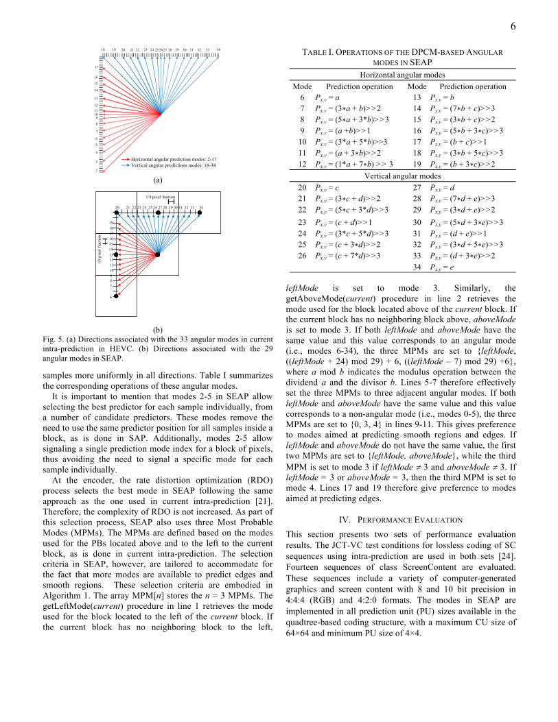
patterns typically occur more frequently than patterns with other directionalities [21]. Therefore, current intra-prediction in HEVC employs a large number of angular modes along these two main directionalities in order to provide more accurate predictions for nearly horizontal and vertical patterns [see Fig 5(a)]. This approach improves current intra-prediction in HEVC particularly for those samples located far from the reference samples. If DPCM-based angular intra-prediction is used, a reduced number of directionalities evenly distributed around the current sample Sx,y should suffice. This is based on the fact that the correlation of a sample with any of its adjacent neighboring samples is usually higher than that with any sample located far in an adjacent block [10]. Therefore, in this work, SEAP uses 29 DPCM-based angular modes to predict directional patterns. Seven angles are defined for each octant, as shown in Fig. 5(b). We employ a more uniform density of prediction modes in all directions compared to that currently employed in HEVC. Specifically, the displacement among angular modes is calculated using 1/8 pixel accuracy. This allows exploiting correlations among neighboring

Fig. 4. Directions used in Mode 5 to predict sample Sx,y according to gradients {G1, G2, G3, G4}.

(a) (b)

(c) (d)

(e)

Fig. 3. Mode 4 in SEAP. (a) Predictor p1 uses the gradient between{e, d} to predict diagonal edges. (b) Predictor p2 uses the gradient between {d, c} to predict vertical edges. (c) Predictor p3 uses the gradient between positions {b, c} to predict horizontal edges. (d) Predictor p4: if a diagonal edge runs along {c, Sx,y}, Sx,y is predicted as (b + 2*c + d) >> 2, where more importance is given to c. (e) Predictor p5: Sx,y is predicted as (b – e) >> 1 if a diagonal edge runs along {b, Sx,y, e}.

Sx,y

Sx-1,y-1 Sx,y-1 Sx+1,y-1

Sx-1,y

Sx-2,y-2 Sx,y-2 Sx+2,y-2

Sx-2,y G1 = |Sx-2,y− Sx-1,y|G2 = |Sx-2,y-2− Sx-1,y-1|G3 = |Sx,y-2− Sx,y-1|G4 = |Sx+2,y-2− Sx+1,y-1|

G1 – 0 deg.

G2– 45 deg. G3– 90 deg. G4– 135 deg.

Px,y=p1 b

c d e Px,y=p2

b

c d

Px,y=p3 b

c d

Px,y=p4

b

c d e

Px,y=p5

b

c d e

6

samples more uniformly in all directions. Table I summarizes the corresponding operations of these angular modes.

It is important to mention that modes 2-5 in SEAP allow selecting the best predictor for each sample individually, from a number of candidate predictors. These modes remove the need to use the same predictor position for all samples inside a block, as is done in SAP. Additionally, modes 2-5 allow signaling a single prediction mode index for a block of pixels, thus avoiding the need to signal a specific mode for each sample individually.

At the encoder, the rate distortion optimization (RDO) process selects the best mode in SEAP following the same approach as the one used in current intra-prediction [21]. Therefore, the complexity of RDO is not increased. As part of this selection process, SEAP also uses three Most Probable Modes (MPMs). The MPMs are defined based on the modes used for the PBs located above and to the left to the current block, as is done in current intra-prediction. The selection criteria in SEAP, however, are tailored to accommodate for the fact that more modes are available to predict edges and smooth regions. These selection criteria are embodied in Algorithm 1. The array MPM[n] stores the n = 3 MPMs. The getLeftMode(current) procedure in line 1 retrieves the mode used for the block located to the left of the current block. If the current block has no neighboring block to the left,

leftMode is set to mode 3. Similarly, the getAboveMode(current) procedure in line 2 retrieves the mode used for the block located above of the current block. If the current block has no neighboring block above, aboveMode is set to mode 3. If both leftMode and aboveMode have the same value and this value corresponds to an angular mode (i.e., modes 6-34), the three MPMs are set to {leftMode, ((leftMode + 24) mod 29) + 6, ((leftMode – 7) mod 29) +6}, where a mod b indicates the modulus operation between the dividend a and the divisor b. Lines 5-7 therefore effectively set the three MPMs to three adjacent angular modes. If both leftMode and aboveMode have the same value and this value corresponds to a non-angular mode (i.e., modes 0-5), the three MPMs are set to {0, 3, 4} in lines 9-11. This gives preference to modes aimed at predicting smooth regions and edges. If leftMode and aboveMode do not have the same value, the first two MPMs are set to {leftMode, aboveMode}, while the third MPM is set to mode 3 if leftMode ¹ 3 and aboveMode ¹ 3. If leftMode = 3 or aboveMode = 3, then the third MPM is set to mode 4. Lines 17 and 19 therefore give preference to modes aimed at predicting edges.

IV. PERFORMANCE EVALUATION This section presents two sets of performance evaluation results. The JCT-VC test conditions for lossless coding of SC sequences using intra-prediction are used in both sets [24]. Fourteen sequences of class ScreenContent are evaluated. These sequences include a variety of computer-generated graphics and screen content with 8 and 10 bit precision in 4:4:4 (RGB) and 4:2:0 formats. The modes in SEAP are implemented in all prediction unit (PU) sizes available in the quadtree-based coding structure, with a maximum CU size of 64×64 and minimum PU size of 4×4.

(a)

(b) Fig. 5. (a) Directions associated with the 33 angular modes in current intra-prediction in HEVC. (b) Directions associated with the 29 angular modes in SEAP.

TABLE I. OPERATIONS OF THE DPCM-BASED ANGULAR MODES IN SEAP

Horizontal angular modes Mode Prediction operation Mode Prediction operation

6 Px,y = a 13 Px,y = b 7 Px,y = (3∗a + b)>>2 14 Px,y = (7∗b + c)>>3 8 Px,y = (5∗a + 3*b)>>3 15 Px,y = (3∗b + c)>>2 9 Px,y = (a +b)>>1 16 Px,y = (5∗b + 3∗c)>>3

10 Px,y = (3*a + 5*b)>>3 17 Px,y = (b + c)>>1 11 Px,y = (a + 3∗b)>>2 18 Px,y = (3∗b + 5∗c)>>3 12 Px,y = (1*a + 7∗b) >> 3 19 Px,y = (b + 3∗c)>>2

Vertical angular modes 20 Px,y = c 27 Px,y = d 21 Px,y = (3∗c + d)>>2 28 Px,y = (7∗d + e)>>3 22 Px,y = (5∗c + 3*d)>>3 29 Px,y = (3∗d + e)>>2 23 Px,y = (c + d)>>1 30 Px,y = (5∗d + 3∗e)>>3 24 Px,y = (3*c + 5*d)>>3 31 Px,y = (d + e)>>1 25 Px,y = (c + 3∗d)>>2 32 Px,y = (3∗d + 5∗e)>>3 26 Px,y = (c + 7*d)>>3 33 Px,y = (d + 3∗e)>>2

34 Px,y = e

24232221201918

14

13

12111098

252627 28 29 30

7

6

5

4

3

2

16

15

17

31 32 33 34

Horizontal angular prediction modes: 2-17Vertical angular predictions modes: 18-34

20 21 22 23 24 25 26 27 28 29 30 31 32 33 34

1/8 pixel fraction

1/8

pixe

l fra

ctio

n 17

1918

13

1516

1110

12

6

789

14

7

Our previous work in [7] has shown that among several DPCM-based methods, SAP-E and SAP+SWP2+DTM attain the best lossless coding performance for a variety of SC and camera-captured sequences compared to current intra-prediction and RDPCM, which is the DPCM-based method standardized in HEVC. Therefore, the first set of evaluation results (Section IV.A) compares SEAP, SAP-E, and SAP+SWP2+DTM with RDPCM. These compared methods are implemented by modifying the HEVC reference software HM-16.6+SCM5.0 [25]. In this first set, the coding tools introduced in the SCC extensions, i.e., IBC, PAL, CCP, and ACTs, are not used in order to determine the coding improvements obtained exclusively by DPCM-based intra-prediction. This first set of results therefore allows demonstrating the effectiveness of SEAP in predicting screen content compared to other DPCM-based intra-prediction methods.

The second set of evaluation results (Section IV.B) compares the lossless coding improvements attained by SEAP when the SCC tools are enabled. In this set, we use the All-Intra (AI) main SCC profile of reference software HM-16.6+SCM5.0 [25].

A. Evaluation of SEAP and various DPCM-based intra-prediction methods

Table II summarizes the performance achieved by the different DPCM-based intra-prediction methods in terms of bit-rate differences, in percentage, with respect to RDPCM. Negative numbers indicate a decrease in bit-rate. As expected, SAP-E and SAP+SWP2+DTM provide very competitive

results for all sequences. Out of these two methods, SAP-E provides the highest bit-rate reductions. Compared to RDPCM, SAP-E provides an average further improvement of 1.36% and 2.45% over SAP+SWP2+DTM, for 4:4:4 and 4:2:0 sequences, respectively.

SEAP attains the highest bit-rate reductions for those sequences where strong edges and discontinuities appear frequently. For example, for sequences missionControlClip3 and console, SEAP outperforms SAP-E by a further 2.34% and 3.35%, respectively, with respect to RDPCM. Fig. 6 depicts the distribution of modes for the first component of three example frames of the console, missionControlClip3 and robot sequences. Each distinct color in this figure represents the proportion of PBs predicted using each mode. The most frequently used modes for the case of sequence console are modes 3, 1 and 27 (pure vertical, see Table I). This is expected, as this component is characterized for depicting numerous strong vertical edges (e.g., plots), edges in other directionalities (e.g., text), and smooth regions. A similar distribution of modes is observed for the entire sequence. For the case of sequence missionControlClip3, the pure vertical mode and mode 1 are used most frequently due to the camera-captured material depicted in the frame. A similar distribution of modes is also observed for the entire missionControlClip3 sequence. For sequence robot, the most frequently used modes are 19, 3 and 15, as the depicted material resembles that of camera-captured sequences with various directional patterns. A similar distribution of modes is also observed for the entire robot sequence. This confirms the effectiveness of using modes specifically aimed at predicting strong edges, as well as those aimed at predicting smooth regions and directional patterns.

TABLE II. LOSSLESS BIT-RATE DIFFERENCES (%) OF DCPM-BASED METHODS COMPARED TO RDPCM

Sequence – precision in bits SAP-E SAP+SWP2+DTM

SEAP

4:4:4 sequences – RGB flyingGraphics – 8 bits -5.59 -4.27 -5.42 desktop – 8 bits -7.46 -6.00 -10.72 console – 8 bits -16.21 -8.32 -19.56 webBrowsing– 8 bits -5.13 -4.82 -7.05 map – 8 bits -5.46 -4.32 -5.14 programming – 8 bits -2.22 -1.29 -4.17 robot – 8 bits -3.40 -2.43 -2.62 EBURainFruits – 10 bits -2.11 -4.68 -5.21 kimono – 10 bits -3.39 -2.64 -1.67

Average for 4:4:4 sequences -5.66 -4.31 -6.84 4:2:0 sequences

missionControlClip3 – 8 bits -5.41 -3.68 -7.75 slideShow – 8 bits -10.97 -5.65 -11.67 basketballScreen – 8 bits -5.18 -4.48 -7.62 missionControlClip2 – 8 bits -6.13 -1.70 -8.27 chinaSpeed – 8 bits -4.58 -4.51 -7.22

Average for 4:2:0 sequences -6.45 -4.00 -8.51

Algorithm 1. Selection of three MPMs for current block 1: leftMode = getLeftMode(current) 2: aboveMode = getAboveMode(current) 3: if leftMode = aboveMode then 4: if leftMode > 5 then 5: MPM[0] ← leftMode 6: MPM[1] ← ((leftMode + 24) mod 29) + 6 7: MPM[2] ← ((leftMode – 7) mod 29) + 6 8: else 9: MPM[0] ← 0

10: MPM[1] ← 3 11: MPM[2] ← 4 12: end if 13: else 14: MPM[0] ← leftMode 15: MPM[1] ← aboveMode 16: if leftMode ¹ 3 AND aboveMode ¹ 3 then 17: MPM[2] ← 3 18: else 19: MPM[2] ← 4 20: end if 21: end if

8

For those sequences depicting screen content combined with a large amount of textures and patterns similar to those found in camera-captured material, SEAP attains very competitive results. For example, for sequence robot, the bit-rate difference attained by SEAP is only 0.78% lower than that attained by SAP-E. As mentioned before, directional patterns are most frequently observed in this sequence. Therefore, the large number of DPCM-based angular modes in SAP-E are particularly effective in accurately predicting these patterns. For sequences map and flyingGraphics, SEAP attains a very similar performance to that attained by SAP-E. The small performance differences, i.e., 0.32% and 0.17% respectively, indicate that the edges and discontinuities in these sequences can be effectively predicted using the DPCM-based angular and edge prediction modes available in SAP-E. This suggests that these sequences depict content that resembles that usually found in camera-captured material.

For sequence kimono, which depicts exclusively camera-captured material, SAP-E outperforms all compared methods. This is expected, as the large number of angular modes in SAP-E are particularly useful to predict the textures and directional patterns of this sequence.

Overall, SEAP provides the largest average bit-rate improvements compared to RDPCM, with average bit-rate reductions of 6.84% and 8.51% for 4:4:4 and 4:2:0 sequences, respectively. These bit-rate reductions are up to 19.56% (see results for console sequence).

B. Evaluation of SEAP using SCC tools Table III tabulates lossless compression ratios attained by

SEAP when employed in conjunction with each of the SCC tools. This table also tabulates bit-rate differences, in percentage, with respect to employing each of the SCC coding tools with no SEAP. For example, column labeled SEAP+CCP tabulates lossless compression ratios attained by SEAP when CCP is enabled as well as the corresponding bit-

rate differences compared to using CCP with current intra-prediction. Column labeled SEAP+ALL tabulates results for the case of enabling all SCC tools. The bit-rate differences in this column are tabulated with respect to using all SCC tools with current intra-prediction. The last two columns of this table tabulates bit-rate differences of SEAP+ALL compared to using RDPCM with all SCC tools (RDPCM+ALL) and SAP-E with all SCC tools (SAP-E+ALL). Results tabulated in these last two columns allow evaluating the effectiveness of SEAP as an alternative to RDPCM when all SCC tools are enabled; as well as comparing SEAP+ALL against SAP-E+ALL, which is the DPCM-based intra-prediction method that outperforms SEAP in some of the test sequences, as tabulated in Table II.

For 4:4:4 sequences, SEAP+CCP and SEAP+ACTs attain the largest average bit-rate reductions compared to their respective counterparts (14.14% and 14.59%, respectively). Note that for sequences flyingGraphics and console, SEAP+PAL attains relatively small bit-rate improvements of 0.84% and 0.48%, respectively, compared to using PAL with current intra-prediction. This indicates that PAL is very efficient in signaling the very limited number of colors depicted in these sequences. As a consequence, using SEAP in conjunction with PAL offers little room for coding improvement. For example, for sequence console, the compression ratio attained by current intra-prediction+PAL is 1:46.55, while that attained by SEAP+PAL is 1:46.77.

When all tools are enabled, SEAP provides an average bit-rate reduction of 8.75% for 4:4:4 sequences, compared to current intra-prediction. Compared to RDPCM+ALL, SEAP+ALL attains an average bit-rate reduction of 3.35%. Note that these bit-rate reductions are maximum for sequence map (6.16%). This particular sequence depicts a limited number of repetitive patterns and textures that can be effectively predicted using IBC. Similarly, it also depicts a limited number of blocks containing a small number of

(a) (b)

Fig. 6. Distribution of modes in SEAP for the (a) Green (G) component of one frame of the console sequence; the (b) Y component of one frame of the missionControlClip3 sequence; and the (c) G component of one frame of the robot sequence. Each distinct color represents the proportion of PBs predicted using each mode.

0

Cross-residual (1)

2

45

6789

HOR (13)11122614151617181920

2122

2324

25

1028

2930

3132 33 34

0 2456

789

HOR (13)11

1226151617

14

1819202122

2324

25

1028 29

30 3132 33 34

0

2

456

78

9

1112

26

151617

14

18

19

2021

22

23

24

25

1028

2930

3132 33 34

9

distinct color values that can be effectively signaled using PAL. SEAP is then able to effectively predict the numerous edges and discontinuities depicted in this sequence, thus improving performance compared to RDPCM+ALL. Compared to SAP-E-ALL, SEAP+ALL attains an average bit-rate reduction of 1.11%. It is interesting to note that, differently from results tabulated in Table II, SEAP+ALL outperforms SAP-E+ALL for most of the tested 4:4:4 sequences. This indicates that the SCC tools, when used in conjunction with SEAP, are capable of improving performance for sequences where SEAP alone is outperformed by SAP-E (for example, see results for sequence robot in Tables II and III).

Overall, employing SEAP with all SCC tools results in higher compression ratios for all 4:4:4 sequences. It is interesting to note that for sequences EBURainFruits and kimono, the attained compression ratios are very similar for all cases. Based on the also very similar bit-rate differences tabulated for these two sequences, these results indicate that the SCC tools, when used individually and collectively, provide a similar coding performance. Indeed, for sequence kimono the compression ratios attained individually by each of the SCC tools with current intra-prediction are {1:3.64, 1:3.63, 1:3.62, 1:3.62} for CCP, ACTs, PAL and IBC, respectively. The compression ratio attained when all SCC tools are used with current intra-prediction is 1:3.64. Consequently, the improvements attained by SEAP when used with the SCC tools, individually and collectively, are relatively constant for these two sequences.

For 4:2:0 sequences, important bit-rate reductions are also observed when SEAP is used in conjunction with each of the

SCC tools. Note that, however, the average bit-rate reductions of SEAP+PAL and SEAP+IBC are greater for these sequences than for 4:4:4 sequences. Since PAL and IBC are designed to exploit, respectively, the limited number of colors and the high occurrence of repeating patterns, they tend to be more effective for the tested 4:4:4 sequence. For the tested 4:2:0 sequences, repeated patterns and blocks with very limited number of colors are not as common as in the tested 4:4:4 sequences. This consequently allows SEAP to provide larger coding improvements for 4:2:0 sequences. This is also reflected on the relatively large bit-rate reductions attained when both PAL and IBC are used in conjunction with SEAP. Specifically, SEAP+ALL provides an average bit-rate reduction of 14.33%, 5.58%, and 1.90% for 4:2:0 sequences, compared to current intra-prediction+ALL, RDPCM+ALL, and SAP-E+ALL, respectively.

The relatively similar compression ratios attained by SEAP with each of the SCC tools for 4:2:0 sequences also indicate that the SCC tools, when used individually and collectively, provide a similar coding performance. For example, for sequence slideshow the compression ratio attained individually by PAL and IBC with current intra-prediction is 1:9.74 and 1:9.86, respectively. The compression ratio attained when both tools are used with current intra-prediction is 1:10.04. SEAP, when used with these SCC tools individually and collectively, attains therefore similar improvements for this sequence, as indicated by the relatively similar bit-rate differences tabulated. Overall, employing SEAP with all SCC tools results in higher compression ratios for all 4:2:0 sequences.

TABLE III. LOSSLESS COMPRESSION RATIOS AND (BIT-RATE DIFFERENCES - %) OF SEAP+SCC TOOLS COMPARED TO CURRENT INTRA-PREDICTION+SCC TOOLS

Sequence–precision in bits SEAP+CCP SEAP+ACTs SEAP+PAL SEAP+IBC1 SEAP+ALL1 SEAP+ALL1 vs.

RDPCM+ALL1

SAP-E +ALL1

4:4:4 sequences – RGB flyingGraphics–8 bits 8.02 (-14.21) 7.70 (-14.74) 10.91 (-0.84) 11.59 (-7.50) 17.51 (-1.53) (-0.62) (-0.18) desktop–8 bits 9.65 (-15.82) 9.48 (-17.03) 30.00 (-4.40) 24.60 (-14.24) 47.76 (-5.42) (-2.95) (-1.46) console–8 bits 23.89 (-26.82) 23.25 (-27.39) 46.77 (-0.48) 33.75 (-16.14) 54.15 (-1.49) (-1.22) (-1.04) webBrowsing–8 bits 9.04 (-13.85) 8.75 (-15.93) 19.24 (-12.32) 18.39 (-15.50) 27.17 (-16.05) (-5.48) (-2.21) map–8 bits 6.57 (-16.94) 6.35 (-17.17) 8.95 (-13.28) 5.65 (-12.87) 10.60 (-15.67) (-6.16) (-0.88) programming–8 bits 5.91 (-13.61) 5.69 (-13.58) 7.01 (-11.00) 7.28 (-15.40) 8.44 (-12.87) (-3.23) (-2.07) robot–8 bits 2.51 (-11.62) 2.43 (-11.59) 2.20 (-10.32) 2.20 (-10.52) 2.55 (-11.38) (-2.60) (-0.02) EBURainFruits–10 bits 3.75 (-9.81) 3.67 (-9.04) 3.67 (-9.04) 3.67 (-9.03) 3.75 (-9.81) (-5.67) (-2.16) kimono–10 bits 3.82 (-4.60) 3.81 (-4.84) 3.81 (-5.00) 3.81 (-4.96) 3.82 (-4.57) (-2.25) (0.02)

Avg. bit-rate differences (-14.14) (-14.59) (-7.41) (-11.80) (-8.75) (-3.35) (-1.11)

4:2:0 sequences missionControlClip3–8 bits 5.27 (-11.73) 6.53 (-12.52) 6.55 (-12.22) (-5.11) (-2.98) slideShow–8 bits 12.03 (-19.00) 12.21 (-19.24) 12.26 (-18.11) (-8.63) (-0.60) basketballScreen–8 bits 6.26 (-14.65) 7.56 (-15.22) 7.57 (-14.70) (-4.59) (-2.04) missionControlClip2–8 bits 4.89 (-12.47) 5.77 (-10.88) 5.77 (-10.81) (-5.37) (-1.75) chinaSpeed–8 bits 3.80 (-16.04) 3.74 (-16.85) 3.80 (-15.80) (-4.18) (-2.14)

Avg. bit-rate differences (-14.78) (-12.45) (-14.33) (-5.58) (-1.90) 1 For IBC, we set the search range to the entire previously encoded region within the current frame.

10

It is important to mention that the coding improvements attained by SEAP+ALL can be further improved if the energy of the residual blocks computed by the DPCM-based modes is reduced. We have recently shown in [7] that this can be attained by applying piecewise mapping functions on the residual blocks so that specific residual values are mapped to unique lower values. As part of our ongoing work, we are applying the ideas introduced in [7] to the modes in SEAP to further improve lossless coding performance when all SCC tools are enabled.

We finish this section with some discussions about the parallelization of the encoding and decoding process in SEAP. At the encoder, all original samples are available for prediction. Therefore, the coding process can be parallelized at the block level. However, at the decoder, the reconstruction process must be performed on a sample-wise manner due to the operations of the modes and the associated inter-dependence of samples. This inevitable hinders the parallelization of the decoding process. It is important to mention that RDPCM offers the advantage of parallelizing the decoding process by allowing the usage of different decoding threads for columns/rows within a block.

C. Encoding and Decoding Times Table IV tabulates the average encoding and decoding time

ratios for the evaluated methods reported in Table II. These time ratios are reported with respect to RDPCM, for each type of sequence. The results in this table show that SAP-E attains shorter encoding times than those attained by RDPCM. Let us recall that RDPCM performs an additional prediction on residual signals after block-wise intra-prediction. This additional prediction is expected to increase encoding times. The longer encoding times of SAP+SWP2+DTM are the consequence of the multiple operations needed to compute the necessary weights of surrounding samples. SEAP only increases encoding times by 0.3% and 1.5% for 4:4:4 and 4:2:0 sequences, respectively. The operations required to find the median values in modes 2 and 4 are the main reason for this increase in encoding times.

Table V tabulates the average encoding and decoding time ratios for all sequences when SEAP is used in conjunction with each of the SCC tools. These average time ratios are obtained with respect to using each of the SCC coding tools with current intra-prediction, as reported in Table III. For example, row labeled SEAP+CCP reports encoding/decoding time ratios with respect to current intra-prediction with CCP. The results in this table show that SEAP tends to increase encoding times for all cases. For cases when SEAP is used in conjunction with each of the SCC coding tools, the increase in encoding times is relatively small, with an average increase of

up to 3.90% (see results for 4:2:0 sequences using SEAP+PAL). Compared to RDPCM+ALL, the increase in encoding times incurred by SEAP+ALL is also relatively small, with an average increase of 2.10% and 3.90% for 4:4:4 and 4:2:0 sequences, respectively. Compared to SAP-E+ALL, SEAP+ALL attains higher encoding times, with an average increase of up to 9.20% for 4:2:0 sequences.

V. CONCLUSIONS This paper presented a collection of DPCM-based intra-

prediction modes for lossless screen content coding in HEVC. This collection of 35 modes, termed SEAP, is aimed at accurately predicting not only textures and patterns similar to those found in camera-captured material, but also strong edges and smooth regions with no sensor noise. SEAP employs modes that allow selecting the predictor for each sample individually from a number of candidate predictors. These candidate predictors are computed based on a casual neighborhood surrounding the target sample. For a block of pixels, SEAP only signals a single mode index to the decoder; therefore, no extra overhead or changes to syntax are needed. Performance evaluations over a variety of screen content sequences indicate that SEAP is particularly effective to predict strong edges and discontinuities. Compared to the standardized RDPCM method, SEAP is capable of attaining bit-rate reductions of up to 19.56%. When all SCC tools are enabled, SEAP provides bit-rate reduction of up to 8.63% compared to RDPCM.

REFERENCES [1] G.J. Sullivan, J.R. Ohm, W.J. Han and T. Wiegand, “Overview of the

High Efficiency Video Coding (HEVC) Standard,” IEEE Transactions on Circuits and Systems for Video Technology, vol. 22, no. 12, pp. 1649-1668, Dec. 2012.

[2] G. Sullivan, P. Topiwala, and A. Luthra, “The H.264/AVC advanced video coding standard: Overview and introduction to the fidelity range extensions,” in Proc. SPIE Int. Soc. Opt. Eng., vol. 5558, pp. 454-474, 2004.

[3] J. R. Ohm, G. J. Sullivan, H. Schwarz, T. K. Tan and T. Wiegand, “Comparison of the Coding Efficiency of Video Coding Standards - Including High Efficiency Video Coding (HEVC),” IEEE Transactions on Circuits and Systems for Video Technology, vol. 22, no. 12, pp. 1669-1684, Dec. 2012.

TABLE IV. ENCODING AND DECODING TIME RATIOS OF DPCM-BASED METHODS COMPARED TO RDPCM

Method Time ratios (%) – encoder/decoder

4:4:4 4:2:0 SAP-E 91.1/94.6 92.0/96.6

SAP+SWP2+DTM 271.7/188.7 270.3/186.7 SEAP 100.3/99.4 101.5/100.0

TABLE V. ENCODING AND DECODING TIME RATIOS OF SEAP+SCC TOOLS COMPARED TO CURRENT INTRA-

PREDICTION+SCC TOOLS

Method Time ratios (%) – encoder/decoder

4:4:4 4:2:0 SEAP+CCP 103.6/101.2

SEAP+ACTs 103.8/102.1 SEAP+PAL 103.5/102.4 103.9/101.2 SEAP+IBC1 101.8/100.0 102.3/100.3 SEAP+ALL1 100.4/99.8 102.0/101.4

SEAP+ALL1 vs. RDPCM+ALL1 102.1/101.3 103.9/101.7

SEAP+ALL1 vs. SAP-E+ALL1 107.0/103.6 109.2/104.3

1 For IBC, we set the search range to the entire previously encoded region within the current frame.

11

[4] J. Xu, R. Joshi, and R.A. Cohen, “Overview of the Emerging HEVC Screen Content Coding Extension,” IEEE Transactions on Circuits and Systems for Video Technology, vol.26, no.1, pp.50-62, Jan. 2016.

[5] D. Flynn, D. Marpe, M. Naccari, T. Nguyen; C. Rosewarne, K. Sharman, J. Sole, and J. Xu, “Overview of the Range Extensions for the HEVC Standard: Tools, IEEE Transactions on Circuits and Systems for Video Technology, vol.26, no.1, pp.4-19, Jan. 2016.

[6] S. Lee, I.-K. Kim, and C. Kim, “RCE2: Test 1 Residual DPCM for HEVC lossless coding,” Joint Collaborative Team on Video Coding (JCT-VC), Doc. JCTVC-M0079, Incheon, Korea, Nov. 2013.

[7] V. Sanchez, F. Aulí-Llinàs, and J. Serra-Sagristà, “Piecewise Mapping in HEVC Lossless Intra-prediction Coding,” IEEE Transactions on Image Processing, 2016, in press.

[8] V. Sanchez, “Sample-based edge prediction based on gradients for lossless screen content coding in HEVC,” in Proc. Picture Coding Symposium (PCS), 2015, pp.134-138, June 2015.

[9] V. Sanchez, “Lossless screen content coding in HEVC based on sample-wise median and edge prediction,” Proc. 2015 IEEE Int. Conference on Image Processing (ICIP2015), pp.4604-4608, Sept. 2015.

[10] M. Zhou, W. Gao, M. Jiang, and H. Yu, “HEVC lossless coding and improvements,” IEEE Trans. Circuits and Systems for Video Tech., vol. 22, no. 12, pp. 1839-1843, Dec. 2012.

[11] M. Zhou and M. Budagavi, “RCE2: Experimental results on Test 3 and Test 4,” Joint Collaborative Team on Video Coding (JCT-VC), Doc. JCTVC-M0056, Incheon, Korea, Nov. 2013.

[12] V. Sanchez, J. Bartrina-Rapesta, F. Aulí-Llinàs, and J. Serra-Sagristà, “Improvements to HEVC Intra Coding for Lossless Medical Image Compression,” in Proc. 2014 Data Compression Conference (DCC), March 2014, p. 423.

[13] V. Sanchez, F. Aulí-Llinàs, J. Bartrina-Rapesta, and J. Serra-Sagristà, “HEVC-based lossless compression of Whole Slide pathology images,” in Proc. 2014 IEEE Global Conference on Signal and Information Processing (GlobalSIP), pp. 297-301, Dec. 2014.

[14] E. Wige, G. Yammine, P. Amon, A. Hutter, and A. Kaup, “Sample-based weighted prediction with directional template matching for HEVC lossless coding,” in Proc. 2013 Picture Coding Symposium, pp. 305-308, Dec. 2013.

[15] Y. H. Tan, C. Yeo and Z. Li. “Residual DPCM for lossless coding in HEVC,” in Proc. 2013 IEEE Int. Conf. Acoustics, Speech Signal Processing (ICASSP), pp. 2021–2025, May 2013.

[16] S.-W. Hong, J. H. Kwak, Y.-L. Lee, “Cross residual transform for lossless intra-coding for HEVC,” Signal Processing: Image Communication, vol. 28, no.10, pp. 1335-1341, Nov. 2013.

[17] G. Jeon, K. Kim, and J. Jeong, “Improved Residual DPCM for HEVC Lossless Coding,” in Proc. 2014 Conf. on Graphics, Patterns and Images (SIBGRAPI2014), pp. 95-102, 2014.

[18] K. Kim, G. Jeon, and J. Jeong. “Improvement of Implicit Residual DPCM for HEVC,” in Proc. 2014 IEEE Int. Conf. Signal-Image Technology and Internet-Based Systems (SITIS2014), pp. 652-658, 2014.

[19] M. Mrak and J. Xu, “Improving screen content coding in HEVC by transform skipping,” in Proc. of the 20th European Signal Processing Conference (EUSIPCO), 2012, pp. 1209-1213.

[20] R. Joshi, J. Sole, and M. Karczewicz, “AHG8: Residual DPCM for Visually Lossless Coding,” Joint Collaborative Team on Video Coding (JCTVC), Doc. JCTVC-M0351, Incheon, Korea, April 2013.

[21] J. Lainema, F. Bossen, W.-J. Han, J. Min, and K. Ugur, “Intra coding of the HEVC standard,” IEEE Trans. on Circuits and Systems for Video Tech., vol. 22, no. 12, pp.1792-1801, Dec.2012.

[22] M. Weinberger, G. Seroussi, and G. Sapiro, “The LOCO-I lossless image compression algorithm: Principles and standardization into JPEG-LS,” IEEE Trans. Image Process., vol. 9, no. 8, pp. 1309-1324, Aug. 2000.

[23] V. Sanchez, M. Hernandez-Cabronero, F. Aulí-Llinàs, and J. Serra- Sagristà, “Fast Lossless Compression of Whole Slide Pathology Images using HEVC,” in Proc. 2016 IEEE Int. Conf. Acoustics, Speech Signal Processing (ICASSP), pp. 1456-1460, March 2016.

[24] H. Yu, R.Cohen, K. Rapaka, and J. Xu, “Common test conditions for screen content coding,” Joint Collaborative Team on Video Coding (JCTVC), Doc. JCTVCT1015, Geneva, CH, Feb. 2015.

[25] HM16.6+SCM-5.0 software. [Online]. Available: https://hevc.hhi.fraunhofer.de/svn/svn_HEVCSoftware/tags/HM-16.6+SCM-5.0rc1/