Doyle - The Economic System (Wiley, 2005)
407
THE ECONOMIC SYSTEM ELEANOR DOYLE
-
Upload
febrian-febri -
Category
Documents
-
view
124 -
download
9
description
ekonomic
Transcript of Doyle - The Economic System (Wiley, 2005)

T H E E C O N O M I C S Y S T E M
E L E A N O R D O Y L E

Copyright 2005 John Wiley & Sons Ltd, The Atrium, Southern Gate, Chichester,West Sussex PO19 8SQ, England
Telephone (+44) 1243 779777
Email (for orders and customer service enquiries): [email protected] our Home Page on www.wiley.com
All Rights Reserved. No part of this publication may be reproduced, stored in a retrieval system ortransmitted in any form or by any means, electronic, mechanical, photocopying, recording, scanning orotherwise, except under the terms of the Copyright, Designs and Patents Act 1988 or under the terms of alicence issued by the Copyright Licensing Agency Ltd, 90 Tottenham Court Road, London W1T 4LP, UK,without the permission in writing of the Publisher. Requests to the Publisher should be addressed to thePermissions Department, John Wiley & Sons Ltd, The Atrium, Southern Gate, Chichester, West SussexPO19 8SQ, England, or emailed to [email protected], or faxed to (+44) 1243 770620.
This publication is designed to provide accurate and authoritative information in regard to the subjectmatter covered. It is sold on the understanding that the Publisher is not engaged in rendering professionalservices. If professional advice or other expert assistance is required, the services of a competentprofessional should be sought.
Other Wiley Editorial Offices
John Wiley & Sons Inc., 111 River Street, Hoboken, NJ 07030, USA
Jossey-Bass, 989 Market Street, San Francisco, CA 94103-1741, USA
Wiley-VCH Verlag GmbH, Boschstr. 12, D-69469 Weinheim, Germany
John Wiley & Sons Australia Ltd, 33 Park Road, Milton, Queensland 4064, Australia
John Wiley & Sons (Asia) Pte Ltd, 2 Clementi Loop #02-01, Jin Xing Distripark, Singapore 129809
John Wiley & Sons Canada Ltd, 22 Worcester Road, Etobicoke, Ontario, Canada M9W 1L1
Wiley also publishes its books in a variety of electronic formats. Some content that appearsin print may not be available in electronic books.
Library of Congress Cataloging-in-Publication Data
The economic system / Eleanor Doyle.p. cm.
Includes bibliographical references and index.ISBN-13 978-0-470-85001-5 (pbk. : alk. paper)ISBN-10 0-470-85001-9 (pbk. : alk. paper)
1. Economics. I. Title.HB171.5.D65 2005330—dc22
2004027116
British Library Cataloguing in Publication Data
A catalogue record for this book is available from the British Library
ISBN-13 978-0-470-85001-5ISBN-10 0-470-85001-9
Typeset in 11/15 New Baskerville by Laserwords Private Limited, Chennai, IndiaPrinted and bound in Great Britain by Scotprint, Haddington, East LothianThis book is printed on acid-free paper responsibly manufactured from sustainable forestryin which at least two trees are planted for each one used for paper production.

C O N T E N T S�
�
�
�
Chapter 1 The Economic System 1
Chapter 2 Market Analysis: Demand And Supply 35
Chapter 3 Beyond Demand: Consumers in the Economic System 77
Chapter 4 Beyond Supply: Firms in the Economic System 113
Chapter 5 Economic Activity: The Macroeconomy 155
Chapter 6 Competition in the Economic System 197
Chapter 7 Money and Financial Markets in the Economic System 239
Chapter 8 Challenges for the Economic System: Unemployment and Inflation 283
Chapter 9 Developing the Economic System: Growth and Income Distribution 321
Glossary 361
Index 387

D E T A I L E D C O N T E N T S
Preface xiii
Acknowledgements xv
Chapter 1 The Economic System 11.1 Introducing the Economic System 11.2 Economic Resources and Markets 21.3 The Economics Approach: Theory-Based Analysis 61.4 Describing and Interpreting Economic Relationships 91.5 Microeconomics and Macroeconomics 14
1.5.1 The Environment for Economic Decisions 161.6 Resource Scarcity and Prices in the Economic System 18
1.6.1 Using Resources and Centralized Decision-Making 201.7 Resource Use, Opportunity Costs and Efficiency 221.8 Alliance of Economic Perspectives 271.9 Positive/Normative Economics 291.10 Summary 30Chapter 1 Appendix 31Review Problems and Questions 31Further Reading and Research 32References 32
Chapter 2 Market Analysis: Demand and Supply 352.1 Introduction 352.2 Exchange – A Central Feature of Markets 362.3 Demand 40
2.3.1 Non-Price Determinants of Demand 422.4 Supply 462.5 Market Interaction: Demand and Supply 52
2.5.1 Changes in Equilibrium 552.6 Government Affecting Prices 56
2.6.1 Price Ceiling 56

viii T H E E C O N O M I C S Y S T E M
2.6.2 Price Floor 572.6.3 Problems of Price Ceilings and Floors 57
2.7 Information and Knowledge in the Market System 582.7.1 Decentralized Decision-Making – The Optimal Form of Organization? 61
2.8 More on Equilibrium in the Demand and Supply Model 632.9 A Market at Work: The Labour Market 64
2.9.1 Labour Demand 642.9.2 Labour Supply: Individual Supply Decision 702.9.3 Equilibrium in the Labour Market 71
2.10 Summary 72Review Problems and Questions 73Further Reading and Research 74References 75
Chapter 3 Beyond Demand: Consumers in the Economic System 773.1 Introduction 773.2 Demand and the Importance of Consumers 78
3.2.1 Consumption Goods 793.3 Consumer Satisfaction – Utility 81
3.3.1 The Assumption of Rationality in Economics 833.4 Marginal Utility, Prices and the Law of Demand 84
3.4.1 The Law of Demand – Income and Substitution Effects 873.5 Demand, Consumers and Consumer Surplus 90
3.5.1 Consumer Surplus and Consumer Welfare 923.6 Consumers’ Response to Price Changes 93
3.6.1 Price Elasticity of Demand 943.6.2 Applications of Elasticity Analysis 983.6.3 Other Elasticity Examples 99
3.7 Consumer Choice and Product Attributes 1013.7.1 The Attribute Model: Breakfast Cereals 101
3.8 Aggregate Consumer Behaviour 1033.9 Government Policies – Consumer Focus 1073.10 Summary 109Review Problems and Questions 110Further Reading and Research 112References 112

D E T A I L E D C O N T E N T S ix
Chapter 4 Beyond Supply: Firms in the Economic System 1134.1 Introduction 1134.2 Firms in Economic Action 1144.3 Why Organize an Economic System Around Firms? 115
4.3.1 Decisions of Firms and the Role of Time 1164.3.2 Firm Revenue 1174.3.3 Firm Output (Product): Marginal and Average Output 1204.3.4 Firm Costs 1234.3.5 Marginal and Average Costs 125
4.4 Maximizing Profits in the Long Run 1314.4.1 Profit Maximization, Normal Profit and Efficiency 1334.4.2 Maximizing Profits Over the Short Run 137
4.5 Supply, Producers and Producer Surplus 1394.6 Producers’ Response to Price Changes 1404.7 Firms’ Investment Behaviour 1424.8 Government Influence on Supply and Production 144
4.8.1 Using Subsidies – An Example with International Trade 1454.8.2 Environmental Taxes – Effects on Production 1474.8.3 Tax Incidence 149
4.9 Summary 150Review Problems and Questions 151Further Reading and Research 153References 153
Chapter 5 Economic Activity: The Macroeconomy 1555.1 Introduction 1555.2 Economic Activity and the Circular Flow 1565.3 Real Output and the Business Cycle 158
5.3.1 Explanations/Causes of Business Cycles 1615.3.2 Implications for Business and Government 165
5.4 Real Output and its Components 1655.4.1 Other Measures of Economic Activity 1675.4.2 Economic Activity: GNP, GDP and Income 168
5.5 Equilibrium Economic Activity 1705.5.1 The Price Level 1715.5.2 Aggregate Demand 172

x T H E E C O N O M I C S Y S T E M
5.5.3 Aggregate Supply 1755.5.4 Bringing AD and AS Together: The Short Run 177
5.6 Equilibrium Economic Activity and the Multiplier 1785.7 International Integration 181
5.7.1 Explaining Growing International Trade 1825.7.2 Benefits and Costs of International Trade 184
5.8 Government Activity 1875.8.1 Another Perspective on Economic Activity: The Economy
as a Production Function 1905.9 Summary 192Review Problems and Questions 193Further Reading and Research 195References 195
Chapter 6 Competition in the Economic System by Edward Shinnick 1976.1 Introduction 1976.2 Competition in the Economic System 198
6.2.1 Competition as a Process 1996.2.2 Entrepreneurship, Discovery and the Market Process 201
6.3 Alternative Models of Competition and Market Structure 2046.3.1 Perfect Competition 2066.3.2 Monopoly 2096.3.3 Perfect Competition vs. Monopoly 2116.3.4 Monopolistic Competition 2136.3.5 Oligopoly 215
6.4 Austrian and Traditional Perspectives: A Comparison 2216.5 When Markets Fail 223
6.5.1 Why Markets May Fail 2236.5.2 Implications of Market Failure 225
6.6 Government Regulation of Competition 2266.6.1 Competition Spectrum 2296.6.2 Structure, Conduct and Performance 2296.6.3 Competition Policy 230
6.7 Summary 236Review Problems and Questions 236Further Reading and Research 237References 237

D E T A I L E D C O N T E N T S xi
Chapter 7 Money and Financial Markets in the Economic System 2397.1 Introduction 2397.2 Money and Exchange 2407.3 Liquidity, Central Banks and Money Supply 242
7.3.1 The Money Multiplier 2447.4 Money Demand 2467.5 The Money Market: Demand and Supply 247
7.5.1 Which Interest Rate? 2487.5.2 Nominal and Real Interest Rates 249
7.6 Quantity Theory of Money and Explaining Inflation 2517.6.1 Inflation Expectations, Interest Rates and Decision-Making 253
7.7 The Foreign Exchange Market 2557.7.1 Demand in the Foreign Exchange Market 2567.7.2 Supply in the Foreign Exchange Market 2567.7.3 Exchange Rate Determination 2577.7.4 Causes of Changes in Exchange Rates 258
7.8 Speculation in Markets 2607.8.1 Investment in Bond Markets 2637.8.2 Bonds, Inflation and Interest Rates 266
7.9 Monetary Policy 2687.9.1 Difficulties in Targeting Money Supply 2697.9.2 Alternative Targets 2707.9.3 Taylor Rules and Economic Judgement 272
7.10 International Monetary Integration 2727.10.1 Considering the Euro 274
7.11 Summary 278Review Problems and Questions 279Further Reading and Research 280References 280
Chapter 8 Challenges for the Economic System: Unemployment and Inflation 2838.1 Introduction 2838.2 Unemployment 284
8.2.1 Labour Market Analysis: Types of Unemployment 2868.2.2 Analysing Unemployment: Macro and Micro 2918.2.3 Unemployment and the Recessionary Gap 2938.2.4 The Costs of Unemployment 295

xii T H E E C O N O M I C S Y S T E M
8.3 Inflation 2968.3.1 The Inflationary Gap 2978.3.2 Trends in International Price Levels 2998.3.3 Governments’ Contribution to Inflation 3038.3.4 Anticipated and Unanticipated Inflation – the Costs 304
8.4 Linking Unemployment and Inflation 3068.4.1 A Model Explaining the Natural Rate of Unemployment 3098.4.2 Causes of Differences in Natural Rates of Unemployment 312
8.5 Cross-Country Differences – Inflation and Unemployment 3148.5.1 Employment Legislation 316
8.6 Summary 317Review Problems and Questions 318Further Reading and Research 318References 319
Chapter 9 Developing the Economic System: Growth and Income Distribution 3219.1 Introduction 3229.2 Living Standards and Labour Productivity Relationships 322
9.2.1 The Dependency Ratio 3279.3 Economic Growth over Time 3319.4 Modelling Economic Growth: The Solow Growth Model 333
9.4.1 More on Savings 3379.4.2 The Solow Model and Changes in Labour Input 3419.4.3 The Solow Model and Changes in Technology 3439.4.4 Explaining Growth: Labour, Capital and Technology 3449.4.5 Conclusions from the Solow Model 3459.4.6 Endogenous Growth 347
9.5 Income Distribution 3499.5.1 Intra-Country Income Distribution 351
9.6 Summary 356Review Problems and Questions 357Further Reading and Research 358References 358
Glossary 361
Index 387

P R E F A C E
A good economics student manages to understand the workings of the componentswithin the economic system. An excellent student manages to appreciate thebroader picture of the system with all its complexity of networks, interrelationshipsand organization. This requires an ability to understand economic models and theirrole in supporting analysis of economic issues plus an appreciation of their usefulnesswhen we attempt to understand economic phenomena at a particular point intime, within their specific, and often complicated, micro- and macroeconomiccontexts. It was with this in mind that I wrote The Economic System. The aim ofThe Economic System is to provide an appropriate mix of topical and historical,practical and theoretical principles of economics that create a tool-box appropriatefor understanding, analysing and addressing the economic issues that we face andattempt to understand.
Any writer or reader of economics textbooks, particularly those aimed at theprinciples of economics market, is aware of the variety of alternatives currentlyavailable. The Economic System is novel in that it does not follow a strict compart-mentalization of chapters into microeconomics and macroeconomics distinctionsbut rather groups material appropriate to the central focus of the chapter toguide learning. The essentials of micro- and macroeconomic theory and analysisare provided within a context where their overlap within the ‘economic system’ isemphasized. A key focus of the book is on highlighting the relationships betweenmicroeconomic and macroeconomic analysis in a way that contributes to a betterunderstanding of their intrinsic relationships and to a better appreciation of howthe economic system works.
This approach addresses a limitation I have experienced where often even thosestudents who appear to solidly grasp concepts and models display weaknessesin using them to better understand or analyse problems and to transfer theirapplication to alternative settings or examples. Transferability of concepts is a realchallenge especially for a subject that focuses on being a problem-solving disciplinewhere students should learn skills useful to support decision-making, i.e. criteriafor choosing between alternatives. An explicit aim in The Economic System is to clarifyhow models and concepts in economics are useful as tools that support rigorous,methodical analysis and not simply useful to solve mathematical ‘puzzles’.

xiv T H E E C O N O M I C S Y S T E M
The use of a small number of chapters, nine in total, that focus on relatedmaterial to highlight these system features of the economy achieves this end. Thereare some further topics that could also have been included in the text; however,I followed the view that learning should not be rushed and that understandingwhat is here is a solid foundation for further learning. The activity of informationintegration requires time and to learn and derive knowledge from that informationis a complex cognitive process.
Another novel perspective is included with references to the ‘Austrian approach’to economics and to entrepreneurship activity in particular, which is explained andreferred to several times in the text. This presents students with an interesting focuson the process element of economic analysis as well as the product element providedin the appropriately comprehensive standard neoclassical analysis.
Real world examples and learning features
Also included within the text are many topical issues including globalization,outsourcing, EMU and the advantages and disadvantages of a single currency.Extensive end-of-chapter material is provided including mini case studies, furtherreading and review questions and problems. Students are required to developtheir range of problem-solving, numerical, analytical and argumentative skills ingenerating their answers to these questions.
Online resource package
For students and lecturers, a comprehensive online support package is providedwith the text. The website includes PowerPoint slides, multiple choice questions,weblinks, online glossary, and further review questions and exercises, plus modelanswers to all of the end-of-chapter questions provided.

A C K N O W L E D G E M E N T S
The contribution of a network of individuals made work on the text substantiallymore enjoyable and challenging. Thanks must primarily go to the many studentsin the Principles of Economics BA course at University College Cork who havecontributed to the development of this book and whose feedback has been grate-fully received and much appreciated. The teaching assistants, including KrystleHealy, James Nolan and Rory O’Farrell, who have supplied their expertise to sup-port the course delivery and test-driven the course materials, also deserve specialappreciation.
I am extremely grateful to many colleagues in the Department of Economics, UCCwho have generated a positive working environment where the role of teaching ishighly valued. For providing many references and nuggets to be followed up or justreflected upon throughout this project sincere thanks to Connell Fanning. EdwardShinnick, the author of Chapter Six, whose timely and focused contribution wasvital in achieving the end result, is deserving of many thanks. For valuable andtimely feedback on various chapters that was much appreciated, I must thank EoinO’Leary, Brendan McElroy and Niall O’Sullivan. Thanks to Kay Morrison andEmer Doyle for editorial and proofreading assistance. For support with content anddevelopment of online materials I am very grateful to Eileen O’Sullivan, KrystleHealy and particularly Gerard Doolan who did trojan work.
Staff at Wiley were supportive above and beyond the call of duty and Anna Rowecomes in for particular thanks here along with Deborah Egleton, Rachel Goodyearand Steve Hardman.
Without family support from Fred and Robert, who bore the brunt of ‘book time’,no text would have been possible. Thank you. Any remaining errors of omission orcommission are, of course, mine alone.

C H A P T E R 1
T H E E C O N O M I C S Y S T E M�
�
�
�
L E A R N I N G O U T C O M E SBy the end of this chapter you should be able to:
✪ Define what is meant by an economic system.✪ Describe the roles played by the main players in the system including indi-
viduals, firms and countries.✪ Describe how and why:
• the principle of exchange;
• the existence of markets; and
• the role of pricesare central to understanding how an economic system functions.
✪ Clarify the role played by concepts, theories and models in economic analysis.✪ Explain how rules and laws facilitate and govern decisions within the eco-
nomic system.✪ Illustrate how each of the following concepts:
• scarcity;
• opportunity cost; and
• economic efficiencyunderpins economic analysis.
1 . 1 I N T R O D U C I N G T H E E C O N O M I CS Y S T E M
This chapter provides an introduction to the economic system to illustrate theinterconnectedness between the different participants in and features of an econ-omy, which contribute to economic decisions and outcomes. An economy canaptly be described as a ‘system’ as it relates to the following definitions of what asystem entails:
• a group of interacting interrelated or interdependent elements forming acomplex whole;

2 T H E E C O N O M I C S Y S T E M
• an organized set of interrelated ideas or principles;
• a functionally related group of elements;
• an organized and coordinated method; a procedure.
The main participants and features of an economy are outlined in the chapters thatfollow. The study of economics focuses on identifying and trying to understand thepatterns and relationships between these elements.
To begin it is useful to define what a study of the economic system entails. Itinvolves understanding how:
• the production of goods and services is organized and influenced by individuals,organizations (including companies – both publicly and privately owned, tradesunions, employer groups, etc.) and governments;
• products and services are used to satisfy the requirements of these sameindividuals, households, organizations and government.
Analysis of production includes the consideration of decisions regarding whatis produced and how production decisions are made, which inputs to use inproduction (factors of production) and the way in which they are organizedtogether to produce output. How production meets the demands of buyers is acentral factor in analysis of the economic system.
Factors of production: the resources necessary for production. They include:
• land – all natural resources (including minerals and other raw materials);
• labour – all human resources;
• capital – all man-made aids to production that have been produced (e.g.machines, factories, tools). It is used with labour to produce and/or marketmore goods and services;
• entrepreneurship in business organization and willingness to take busi-ness risks.
1 . 2 E C O N O M I C R E S O U R C E SA N D M A R K E T S
A key focus of economists’ attention is the relationship between an economy’sresources, both in quantity and quality, and what it can produce again in quantityand quality. The concept of efficiency helps in the analysis of this relationship.

T H E E C O N O M I C S Y S T E M 3
Economic efficiency: optimum production given the quantity and quality ofavailable factors of production and their cost.
An economy is efficient if it is maximizing the output it can produce within theconstraints of its available inputs or resources. These constraints may take the formof rules or laws governing how inputs may be used, such as limits to the hourspeople are permitted to work per week.
Economists’ focus on output and production is driven by an inherent interest intrying to understand how society could be better off and this is evident as far back as1776 in An Inquiry into the Nature and Causes of the Wealth of Nations by Adam Smith,the acknowledged ‘father’ of economics. What is produced in an economy has adirect bearing on the income – the flow of money earned – and wealth – the stockof money held – of people in that economy.
When an economy increases the quantity of goods and services it produces andcan sell the output, economic growth occurs.
Economic growth: an expansion in the quantity of goods/services producedand sold.
Once economic growth is faster than population growth, material living standardscan rise.
Living standards: the level of material well-being of a citizen. It is generallymeasured as the value of a country’s production per person, e.g. UK nationaloutput divided by the population of the UK for a particular period of time.
Some data on international living standards are presented in Figure 1.1 for 20countries with the highest living standards in 2002 (as reported by the OECD,the Organization for Economic Cooperation and Development). To ensure thedata reported in Figure 1.1 can be compared, each country’s output was initiallyconverted to the same exchange rate – here all values are in dollars.
Because of the different international prices of goods, a further adjustment wasmade to the data to take account of these purchasing power differences. Thisis called the purchasing power parity adjustment as explained in the text box.Figure A.1 in Chapter 1 Appendix contains living standards data for 2000 over abroader selection of counties.
Purchasing power parity (PPP) is a measure of the relative purchasing power ofdifferent currencies. PPP is the exchange rate that equates the price of a basket

4 T H E E C O N O M I C S Y S T E M
0 10 000 20 000 30 000 40 000 50,000
LuxembourgUSA
NorwaySwitzerland
IrelandCanada
BelgiumDenmark
JapanAustria
AustraliaNetherlands
GermanyFinlandFrance
SwedenUK
IcelandItaly
Spain
F I G U R E 1 . 1 L I V I N G S T A N D A R D S , T O P 2 0 C O U N T R I E S2 0 0 2 , ( U S D O L L A R S A N D P P P s∗ )Source: Main Economic Indicators, OECD, 2002∗See the nearby key term box for more on PPPs.
of identical traded goods and services in two countries. PPP is often very differentfrom the current market exchange rate.
Since 1986 The Economist magazine has published a regular Big Mac Index. Itindicates how many Big Macs dollars buy internationally when exchanged forlocal currencies. The Big Mac PPP is the exchange rate that would leave theBig Mac costing the same in the United States as elsewhere.
The logic underlying conversions using PPPs and not just standard exchangerates is that prices tend to be lower in poor economies, so a dollar of spendingin a poor country buys more than a dollar in America. Using purchasing powerparities takes account of these price differences. Comparing actual exchangerates with PPP often reveals differences. Some studies have found that the BigMac Index is often a better predictor of currency movements than other more‘theoretically rigorous’ currency models.
Since January 2004, The Economist also provides a Tall Latte Index where thefocus is not on burgers but a cup of Starbucks coffee, another internationallyavailable product.

T H E E C O N O M I C S Y S T E M 5
Economists are interested in understanding the reasons behind economies’ growthexperiences and the reasons underlying the cross-country disparity of livingstandards. Several explanations as to why such disparities arise are offered andin our study of the economic system we will touch on some of these.
To fully appreciate how an economy functions also involves an understanding ofthe political context within which economies work as this too has an influence onthe output produced and the available resources.
Political economy is the term given to the study of how the rules, regulations,laws, institutions and practices of a country (or a state, region, province) have aninfluence on the economic system and its features.
Rules and laws on how resources and production can be organized and usedinfluence the incentives for individuals and firms to conduct business and hencethe output of an economy. One example would be rules on setting up new businessesand the time this takes.
Research indicates time needed for setting up a new business varies consider-ably internationally, taking only two days in Canada and costing US$280, and62 days in Italy, costing US$3946 (Djankov, et al., 2001).
Rules and laws on how resources are shared or distributed among citizens alsoinfluence their income and wealth – if only a few receive most of the production(because of corruption or a caste system, for example) the income and wealth ofthe majority suffers.
How the value of output produced is distributed among an economy’s stake-holders depends on the configuration of each economic system and the choiceson distribution that are made. Stakeholders in the economic system are the indi-viduals and groups that depend on the system to fulfil their own goals (be it tomeet demands, generate income, create employment, provide wages or salaries,provide goods and services . . . ) and on whom the economic system depends for itscontinued survival.
According to the above description of what an economy is, it is possible to inter-pret individual countries as economic systems, each with its individual economy,but it may also be useful, depending on some issues of interest to economists, toconsider provinces, regions or cities as economies in their own right.
It is also often useful to examine an economy by focusing on sub-sections oforganized resources within an economy, which are described as markets, e.g. the
6 T H E E C O N O M I C S Y S T E M
market for cars, apples, or labour. Knowledge of how the economic system func-tions based on analysis of markets, production and expenditure decisions and howeconomies grow will help to enhance understanding of why economies perform sodifferently.
Markets: situations where exchange occurs between buyers and sellers or wherea potential for exchange exists. Markets cover the full spectrum from physicallocations where buyers and sellers meet to electronic markets (such as auctionwebsites) facilitated by the Internet.
The familiar notion of a market where people come together in a particular locationto buy and sell goods or services is the most straightforward definition of a market.The economist’s definition is broader and does not limit a market to a specific timeand place.
For example, we can refer to the market for apples, which covers the opportunitiesthat exist for buying and selling apples between individuals and firms. Markets forproducts or services can usually be examined by considering the price at whichproducers or sellers are willing to supply and sell – the supply or production side of amarket – and the price buyers are willing to pay – the demand or consumption sideof a market. Depending on the price of a product (amongst other factors) sellersand buyers make their economic decisions about which products to produce/buyand the quantities to produce/buy. The model of demand and supply presentedin Chapters 2, 3 and 4 and again in Chapter 6 develop these two elements of theeconomic system further.
The basic elements of the economic system therefore, involve, the organizationof production and supply, consumption and demand, markets, exchange, prices,and the rules or laws that facilitate and govern decisions by individuals, householdsand firms relating to all of these elements.
1 . 3 T H E E C O N O M I C S A P P R O A C H :T H E O R Y- B A S E D A N A LY S I S
In recent years the scope of economics has expanded considerably due to thebreadth of applications that are possible based on the concepts, theories andmodels that constitute the foundations of the discipline.
Concepts, theories and models are simplified representations of phenomena,which are intended to serve as tools to aid thinking about complex entitiesor processes.

T H E E C O N O M I C S Y S T E M 7
T A B L E 1 . 1 E C O N O M I C T H E O R Y A N D T H E P R O C E S S O FE C O N O M I C A N A LY S I S
1. Identify a question/issue for analysis, e.g. the factors that explain why Luxembourg hasrelatively high living standards at a point/period in time.
2. Identify theory (and/or concepts and/or models) relevant to this issue, e.g. theory ofeconomic growth that relates output and living standards to the quantity and quality ofavailable factors of production.
3. From theory, formulate hypotheses about possible relationships between high living stan-dards and high levels of education (affecting labour), investment (affecting capital) etc., e.g.one hypothesis would be that high living standards are caused by high levels of education.
4. Test the hypotheses against evidence (information/data) on high living standards inLuxembourg and competing potential explanations. From alternative explanations – e.g.education, investment, luck! – the economist must attempt to choose the most appropriateand convincing, given available evidence. To get to the root of the analysis it may also benecessary to focus on the causes of high levels of education or investment, which is notstraightforward. If the cause of high levels of education (or investment) is high levels ofincome/living standards then the explanation is circular and is not very useful. Evidence usedto test an hypothesis might be quantitative (numerical), or qualitative or a mixture of both,and might be published or might be collected by the economist themselves in interviews orsurveys, for example.
5. Draw valid conclusions.
What constitutes what economists do is as much governed by the approach toanalysis they use as by the issues they examine. Table 1.1 provides a frameworkillustrating how theory guides economic analysis.
An economic method of analysis involves using concepts, theories and models(that are transferable to a multitude of issues), which serve to structure thinkingand clarify the fundamental features of interest in addressing an economic issueor answering an economic question. This method helps economists identify andorganize the main features causing an economic phenomenon and perhaps rankthe most important causes and effects and essentially to understand the mostimportant features that explain how economies actually work. It is not sufficientto identify correlations between economic phenomena – high standards of livingand education – because correlation is not causation! Overly focusing on datarelationships without an underlying logical theory of causation is bad economicsand does not give rise to valid conclusions. In relation to the example in Table 1.1

8 T H E E C O N O M I C S Y S T E M
the essence of the issue is whether living standards in Luxembourg would be higheror lower at a particular time with different levels of education (or investment).
Models are sometimes criticized because of how they simplify reality but theyare constructed in order to take into account the most important features of theeconomic system relevant to analysing a specific issue. For example, the standardeconomic model of supply and demand abstracts from all the various factors thatfeed into the determination of supply and demand to focus on the relationshipbetween the price of a product and
• producers’ decisions of how much to supply at different prices (supply);
• buyers’ decisions of how much to purchase at different prices (demand).
Supply: the quantity of output sellers are willing to sell over a range of poss-ible prices.Demand: the quantity of output buyers are willing to buy over a range ofpossible prices.
The demand/supply model is the cornerstone of economic analysis (and isdescribed in detail in Chapter 2) and is used throughout this book. We canacknowledge that a number of different factors feed into the decisions that sup-pliers (producers) make regarding what to produce, in what quantity and what priceto charge. These decisions would take into account producers’ available resourcesof money, machinery, production technology and know-how.
In their theories and models, economists abstract from all other factors toconsider the essence of how economic units or phenomena are related. In focusingon the relationship between price and demand, for example, we consider howdemand relates to price and price alone. The approach treats all the other potentiallyintervening factors as if they were unchanging, allowing one relationship to beconsidered in isolation. This method followed by economists is described as theceteris paribus assumption.
The ceteris paribus assumption: from the Latin the direct meaning of this term isall things being equal or unchanged.
This could be rephrased as the ‘economists are not stupid’ assumption!Economists know all things do not remain equal or unchanged. The power ofthe assumption allows them to construct models that highlight the fundamentalnature of a relationship they are trying to describe and understand. Subsequentlythey use their models to incorporate other factors of most relevance to thatrelationship.

T H E E C O N O M I C S Y S T E M 9
Economic analysis of demand can be extended to consider, for example, the effectthat a general rise in income would have on a people’s decision regarding Demand.In the case where consumers’ incomes rise, ceteris paribus, we would expect rationalconsumers to buy more apples, or beans or CDs for example – more on this inChapter 2! The objective of the model of demand is, therefore, not to simplifyreality and assume that price is the only factor that feeds into consumers’ decisionsbut to create a model whereby the analysis of any factor that is relevant can beconsidered in a clear and concise framework.
Many models are used in economics, which serve similar purposes of allowing thecomplexity of an economic issue to be understood and sometimes future behaviour(e.g. of suppliers or buyers, or economies) to be predicted. Clearly, despite theirmodels and concepts, economists do not always predict future behaviour or out-comes correctly. Just like weather prediction, the models do not always allow forall relevant factors that affect the outcome to be considered or in some casesprobabilities of occurrences are under/overestimated. This is due to the inherentuncertainty in trying to predict economic outcomes that arise due to individualbehaviour and decision-making. It is precisely because the future is uncertain thateconomists try to argue logically which potential outcomes are most likely or not.
1 . 4 D E S C R I B I N G A N D I N T E R P R E T I N GE C O N O M I C R E L AT I O N S H I P S
In attempting to draw sound conclusions, economists often use facts and figures totest their economic arguments. They compute percentages, they use index numbers,draw and manipulate diagrams and they analyse trends in data over time. If you arecomfortable with such activities, you should skip this section.
To compute a percentage we are interested in the proportionate change in aquantity or value. Saying that employment increased by 10 000 jobs does not provideas much information as if you know what the initial level of employment was.
Consider an economy where 125 000 people are employed. Increasing jobs by10 000 represents a percentage increase of 8% which is found by:
Percentage change = (Change/initial value)∗100
In this example the relevant figures are (10 000/125 000)∗100 = 8%

10 T H E E C O N O M I C S Y S T E M
With data on changes in employment produced monthly and quarterly in manyeconomies it would be possible to compute percentage changes over these periodsand examine whether the general trend were up or down, or whether any pat-terns emerged such as seasonal increases – temporary summer workers are usuallyemployed for a few months and then are laid off, students return to college,etc. – and this affects employment figures.
Alternatively, quantities or values can be expressed in index number form allow-ing them to be presented relative to one base point in time. Consider UK employ-ment statistics. Table 1.2 shows employment between 1999 and 2003 based to 1999 =100. By setting a base year value (1999 = 100) it is easy to read off the relative percent-age changes in employment, which declined for both women and men across man-ufacturing industries. The total figure is the weighted average of men and women.
In 1999 men represented 72% of the workers while women accounted for theother 28%. Taking a weighted average of 72% of the 1999 value for men and28% of the value for women gives 100 overall (0.72∗100 + 0.28∗100 = 100).The same weights apply for 2000 and 2001 and changed to 73% and 27% forthe final two years.
Index numbers are commonly used in describing trends in prices and in weightedaverages of prices, such as the retail price index, consumer price index, wholesaleprice index. Assessing changes in prices is important for all economic analyses ofany variables measured in money terms over time – income, output, wages and so
T A B L E 1 . 2 E M P L O Y M E N TS T A T I S T I C S M A N U F A C T U R I N GI N D U S T R I E S : I N D E X N U M B E R S
Year Total Men Women
1999 100 100 100
2000 98 98 97
2001 93 94 92
2002 88 89 86
2003 85 86 82

T H E E C O N O M I C S Y S T E M 11
on. To see why this is so take the example of a car firm that produced £500m worthof output in 1990 and £800m in 2000. These amounts are in nominal or current termswhich means they are the actual value of production not adjusted for price changes.Without further investigation you might consider that the economic activity of thefirm increased over time since its output expanded by £300m or 60%. However, ifyou knew that over the same period average output prices increased too then withoutfurther information it is impossible to know what proportion of the extra 60% is dueto rising prices or to any additional quantity of output. If prices rose by 60% then thefirm’s quantity of output would not have changed at all – only its monetary value.
It is possible to disentangle the two separate effects of price and quantity if weknow the extent of the price rise over time. Assume it is 25% relative to pricesin 1990. Essentially what is required is to quote output values in real terms so thatthe effect of price changes is removed and only quantity or real effects remain, asexplained in the text box.
Nominal and real amounts: price and quantity effects
Changes in nominal amounts are made up of price and quantity effects.Economists are concerned with quantity effects.
e.g. Nominal change in value of output = change in price∗change in quantity
In the above example the nominal change in the value of output is £300m.Using 1990 as a base year we can compute the following:
Nominal output index 1990 = 100 2000 = 160 [1990 = 500 2000 = 800]Price index 1990 = 100 2000 = 125
A corresponding quantity index is found by dividing the nominal output indexby the price index, i.e. (160/125)∗100.
Quantity index 1990 = 100 2000 = 128 [1990 = 500 2000 = 640]
To double-check this is correct, the product of the volume and price indicesshould equal the total change in the nominal index (128∗125)/100 = 160.
The real value of output in 2000 expressed in 1990 prices was £640m, representinga 28% increase in the quantity or volume of output.

12 T H E E C O N O M I C S Y S T E M
10 00012 00014 00016 00018 00020 00022 00024 00026 00028 000
0 1 2 3 4 5 6Household size in persons
Ele
ctri
cty
cons
umpt
ion
kWh
F I G U R E 1 . 2 E L E C T R I C I T Y C O N S U M P T I O N A N DH O U S E H O L D S I Z ESource: Statistics Norway, 2004
Diagrams provide some indication of whether relationships exist betweenvariables. For example, using data on average household size and electricity con-sumption indicates if and how both are related. Sample data are shown in Figure 1.2and were taken from Statistics Norway. Such data are known as cross-section dataas they provide information on different variables for one point in time (Figure 1.1also shows cross-section data).
If data on electricity consumption were available over a number of time periodsthey would be called time-series data. For different household sizes (number ofpersons in the household) we see that smaller households had lower electricityconsumption (measured in kilowatts per hour).
Linear relationships apply between many economic variables. In practice rela-tionships are approximately linear as shown by the trend line added to the data pointsin Figure 1.2. The trend line approximately describes the relationship since onlyone data point actually sits on the line (a standard spreadsheet package was used toconstruct the line). For any linear relationship if the causal variable (X) changes italways brings about the same or constant effect on the variable it affects. Usually inmathematics, the causal or independent variable is put on the horizontal or X-axiswhile the dependent variable is on the Y-axis.
To draw a line we need:
1. The value of the dependent variable irrespective of the value of the causal orindependent variable. This is called the intercept of the line.

T H E E C O N O M I C S Y S T E M 13
2. A measure of how one variable reacts to changes in the causal variable. This iscalled the slope of the line.
A standard general expression for a line is presented and explained in the text box.
General expression for a line: Y = c + mX where
• Y denotes one variable, e.g. electricity consumption;
• c denotes the intercept, i.e. the value of Y irrespective of the value of X;
• m denotes the extent to which Y changes as X changes, i.e. how electricityconsumption varies with household size;
• X denotes the variable causing changes to Y, e.g. household size.
The specific line described in Figure 1.1 is Y = 10759 + 3220.5XElectricity consumption is 10 759 kWh irrespective of household size andincreases by 3220.5 with each additional one-person increase in household size.
From this relationship it is possible to predict what electricity consumptionwould be if household size were seven (ceteris paribus!).
Y = 10759 + 3220.5 × 7 = 10759 + 22543.5 = 33302.5
Figure 1.2 is an example of a positive relationship because both variables movein the same direction and it is reflected in an upward sloping line. For negativerelationships Y would fall if X rises, and rise if X falls, for example the relationshipbetween the quantity of hours of sunshine per day and the quantity of umbrellaspurchased.
Not all economic relationships are linear. For example, the price you pay forapples might be lower if buying in bulk from a grower. The more bought, the lowerthe unit price the grower quotes – why might a grower behave in this way? Thereaction of quantity bought to changes in price may not be in constant proportionso that for each extra 10% decline in the price the quantity purchased increases atan increasing rate as shown in Figure 1.3.
Here, the 10% drop in price from 30p to 27p increases purchases by 10 appleswhile the 10% drop from 15.94p (to 14.35p) increases purchases by an extra 40apples. Why might a buyer behave in this way?
Although mathematicians usually place the causal (independent) variable on thehorizontal axis, economists by convention place quantity purchased on this axis.This goes back to Alfred Marshall’s treatment of price as the dependent variable

14 T H E E C O N O M I C S Y S T E M
1012141618202224262830
0 50 100 150 200 250 300Quantity purchased
Pri
ce
Price 30.00 27.00 24.30 21.87 19.68 17.71 15.94 14.35 12.91
Quantity 10 20 35 55 85 120 160 210 275
F I G U R E 1 . 3 Q U A N T I T Y P U R C H A S E D A N D P R I C E
and although most economists agree that price is the independent variable, andquantity purchased depends on price, they follow this convention. Alfred Marshall(1842–1924) was Professor of Political Economy at the University of Cambridgefrom 1885 to 1908. He founded the Cambridge School of Economics and taughtrenowned economists including Pigou and Keynes. Marshall’s great work wasPrinciples of Economics (1890), published in eight editions in his lifetime andconsidered the ‘Bible’ of British economics, introducing and explaining conceptsstill conventionally used.
A trend line has been added to Figure 1.3 to indicate how it would approximatethe nonlinear relationship. The curved (nonlinear) trend is also included to showhow it better describes the general pattern of the data.
Further nonlinear relationships are observed between economic variables andwill be met and considered later on in the text.
1 . 5 M I C R O E C O N O M I C SA N D M A C R O E C O N O M I C S
A distinction is made in most economics textbooks between the areas of microeco-nomics and macroeconomics.

T H E E C O N O M I C S Y S T E M 15
Microeconomics: study of the causes and effects of the behaviour of individualeconomic units within the economic system (or groups with broadly similarinterests and goals) such as consumers, producers, trades unions, firms andtheir impact on the markets in which they interact – e.g. the car, apple orlabour markets.Consumer theory assumes consumers wish to maximize their benefit or utility.The theory of the firm assumes producers wish to maximize profits.
Many microeconomic decisions are based on prices, such as consumers’ buyingmore apples if price falls, more people trying to work in the IT sector if wages (theprice of labour) rises and so on. Hence microeconomics is also referred to as pricetheory. In considering economic units economists attempt to model and understandhow the unit or related group of people behaves. Economic units are assumed tobehave rationally, in the sense that they try to achieve the greatest amount ofbenefit, or utility, from their actions. With the assumption of rational behaviour theconsideration of constraints on choices can be modelled in an attempt to estimatean optimal or most efficient outcome. For example, in attempting to increase utilityby buying something I value, I am constrained by my income. I will try to maximizethe utility I get from consumption, given my limited income. Many microeconomicissues are dealt with according to this ‘optimal solution’ method using the supplyand demand model.
Once an analysis of individuals and units can be undertaken, it is possible toconsider how all economic choices fit together and we can move to an analysis ofeconomic aggregates such as aggregate production – not just of apples but of allgoods and services. It is not always possible or feasible to consider the impact of aneconomic event across each of the individual units or markets that it may affect.Macroeconomic analysis is useful instead.
Macroeconomics is the study of:
• The relationships between aggregate or combined elements in the eco-nomic system such as national production and employment, for example.
• Causes of changes in aggregate economic performance including economicstructure and economic institutions.
A model of the macroeconomy based on consumer, producer and governmentaction is presented in Chapter 5.
National exchange rates reflect the price of one country’s currency in termsof other currencies, and inflation rates indicate how average national prices

16 T H E E C O N O M I C S Y S T E M
change over time and these are also examined as macroeconomic issues thataffect economies. Furthermore, from a government’s perspective macroeconomicpolicies constitute a key element in their attempts to maximize the performanceof their economies to achieve policy goals such as high employment and ris-ing incomes and living standards for their citizens. Hence, macroeconomics alsofocuses on the impact of government policies on output, employment, inflation orexchange rates.
Although there has been a traditional division of economics into micro- andmacroeconomics, an understanding of economics requires the appreciation thatthey are not independent of each other. Individuals’ decisions feed into demandand supply in different markets. Aggregate or overall economic activity is clearlydependent on what happens in different markets, which is based on the choicesand behaviour of individuals, firms and economic units regarding what buyerswish to buy and what producers wish to sell, for example.
A key focus of this text is on highlighting the relationships between micro-economic and macroeconomic analysis in a way that contributes to a betterunderstanding of their intrinsic relationships and to a better appreciation of howthe economic system works.
Hence, elements of both microeconomics and macroeconomics that pro-vide useful frameworks for considering related issues are provided throughoutthe book.
1.5.1 THE ENVIRONMENT FOR ECONOMIC DECISIONSRules and laws also impinge on economic choices as rational people react toincentives with which they are faced. For example, interactions between consumersand firms are not independent of such rules because of the regulatory environmentthat exists, i.e. the rules and regulations, including laws, set down by governments inboth national and international contexts which describe how citizens and businessesshould operate.
Trade agreements are established by the international organization called theWorld Trade Organization (WTO) (see www.wto.org). Following prolongeddiscussions between government officials, the agreements are signed by govern-ments. Firms in signatory countries must abide by the set rules and regulationsor face penalties.

T H E E C O N O M I C S Y S T E M 17
Various governments have appointed regulators of competition in attempts topromote greater competition in economies by tackling anti-competitive practices,and so contributing to an improvement in economic welfare. (Alternative marketstructures and their implications for competition, among other issues, are examinedin Chapter 6.) Such practices might include firms:
• agreeing to ‘fix’ prices – not allowing prices to be determined freely in theeconomic system by demand and supply;
• limiting output to create artificial scarcity and keep prices high;
• dividing business between them or abusing their market position with nobenefits to consumers.
Recently the issue of corporate governance has made the headlines because anumber of big companies (e.g. Enron, WorldCom, Parmalat) have revealed poorand/or illegal methods of administration or accounting that resulted in a reductionof confidence in their financial reporting procedures, hence their reported earningsand most importantly their future performance. This impacts on people’s willingnessto invest in companies and may weaken their confidence in the ability of theeconomic system to operate efficiently or fairly.
Confidence and expectations can play an extremely important role in economicsuccess – many surveys and ‘barometers’ of consumer confidence are reported andare considered to be key leading indicators of future economic performance. Forone example, check out http://www.conference-board.org/economics/consumer-confidence/index.cfm. Why is consumer confidence so important? If consumersare not confident about the future, if they are fearful for their jobs they may prefernot to make purchases of goods and services in the immediate future, opting tosave their money rather than spending it on consumer goods.
Consumer confidence: the degree of optimism that consumers express (insurveys, for example) about the state of their economy through their saving andspending patterns.
A worker who thinks their job may be cut will probably put off upgrading their caruntil such time as they feel more secure about their prospects. If consumers are notin the ‘mood’ to buy, firms cannot sell as much of their output as they expectedand so production might fall, leading to lay-offs and in worst-case scenarios sloweconomic growth (or even negative growth) for a period of time.
Appreciating the role played by each of the different components of the economicsystem and how interactions between the components all impact on the outcomes

18 T H E E C O N O M I C S Y S T E M
within the system itself is a key goal that guides this book. A good student managesto understand the workings of the components within the economic system. Anexcellent student manages to appreciate the broader picture of the system withall its complexity of networks, interrelationships and organization. This requiresan ability to understand economic models and their role in supporting analysisof economic issues plus an appreciation of their usefulness when we attempt tounderstand economic phenomena at a particular point in time, within their specific,and often complicated, context.
1 . 6 R E S O U R C E S C A R C I T Y A N D P R I C E SI N T H E E C O N O M I C S Y S T E M
A key issue that motivates the study of economics is how to resolve the discrepancybetween scarce resources and the numerous potential uses for them (and how thisis actually ordered and organized via the economic system). Resources are clearlyscarce in the sense that we, the world’s citizens, cannot fulfil all our economicdesires, given our share of available resources. This arises to an extent because ofdifficult-to-defend policies on the distribution of income in some economies (whichis discussed in Chapter 9). It arises also since some resources are finite – such asoil, gas, etc. – although new inventions and innovations allow new products to bedeveloped constantly thus pushing out the boundaries we see for many resources (asJulian Simon explains in his article at http://www.cato.org/dailys/3-04-97.html).We make choices based on preferences regarding how and when we use ouravailable resources to satisfy not simply our needs but our desires, and moregenerally throughout the economic system, choices are made based on subjectivedesires of individuals, companies and governments.
Choice inevitably involves precluding alternatives. Using resources in a particularway means those resources are unavailable for simultaneous use in another way sincean opportunity cost is incurred. If I use all income on food I cannot buy clothes, orif I establish a manufacturing plant for tables it is not suitable for making chemicals.
Opportunity cost: This is the cost of what is given up in following one course ofaction such that other choices are no longer possible. It is subjective and can beestimated in terms of the cost of the next-best preferred alternative but only whenthe choice made cannot be reversed.
It is via the economic system that decisions about how resources are used are made bythe many buyers and sellers in markets. While we can view the economy as a system,

T H E E C O N O M I C S Y S T E M 19
the economic decisions made within that system are based on human behaviourand preferences. At the heart of economic decision-making is the necessity toselect between alternatives. In making a choice, decision-makers should be awareof the costs of their actions in terms of what they cannot do once they make oneparticular choice, i.e. the opportunity cost of their decision to ensure the best – mostefficient – use of scarce resources.
Consumers decide what to buy with their available income, and how muchshould be saved rather than spent, based on available information. For example,consumers’ decisions about what to buy depend on the prices and availability ofvarious products, their personal tastes, needs and available income (in no specificorder). Employment choices depend on the jobs that are available, on individuals’qualifications and abilities and the wage rate. Firms also make economic decisions asthey attempt to produce and sell their products or services (at prices that consumersare willing to pay) basing their decisions on perceptions of what is happening intheir market, which is affected by consumers’ demands, the available productiontechnologies, the firm’s know-how, and how competing firms behave. A firm’schoices are, therefore, bound up in the network of decisions that result in whatpotential buyers want and what other firms are doing to compete.
Decision-making by individuals and firms is facilitated by the prices they observe inmost markets. This means that prices play a central role by signalling information toconsumers regarding how best they should use their available resources (includingmonetary, entrepreneurial, land and labour resources). Prices also act as a signalto producers of the price they can expect to earn for their products which will leadthem to make particular decisions about what inputs to use (employees, machines,computers, etc.) how much they can afford to pay for inputs and so on. Hence, theprice mechanism provides a means for coordinating the goals and choices of thevarious decision-makers in a market-based economic system.
Interestingly, from an objective point of view, not all economic outcomes mightbe considered to enhance the overall well-being of society. Take for instancethe fashions that lead to rising expenditure on mobile phones and theiraccessories that might, arguably, be better spent on improving education orhealth. Instead of allowing the market system to organize the use of resourcesand what is produced based on the price mechanism and individuals’ andcompanies’ responses to prices, it would be possible to consider handing overtotal control for such choices to an ultimate decision-maker who ‘knows best’.But this would not necessarily lead to a better overall outcome. Economists

20 T H E E C O N O M I C S Y S T E M
consider that it is through the dispersed decision-making by individuals andorganizations in the economic system that the best use of dispersed economicknowledge regarding demands, supplies and markets is facilitated which allowsprices to act as signals to all participants in the system. This highlights oneissue at the heart of economic debate – the costs and benefits of centralizedversus dispersed decision-making.
Economists argue that centralized decision-making about how resources shouldbe used and what products should be produced leads to inefficient resource usewhere surpluses of some goods and shortages of others would be created (as inmany former centrally planned economies). Furthermore, such systems take awayindividuals’ freedom of choice. In fact, the dependence of a substantial proportionof our market-based economic system on the price mechanism actually means thatindividuals’ choices are affected by the choices and decisions of other membersof the system. This happens because the sum total of all individual choices (byproducers on the supply side of the economy and buyers on the demand side)feed into the economic system to generate the market prices we observe (analysedin detail in Chapter 2). Hence, subsequent decisions by buyers and sellers aredisciplined and organized by the price mechanism. This is what Adam Smithalluded to in his discussion of the invisible hand that guides the economy – aguiding mechanism that is no one individual’s responsibility, desire or goal, but isthe outcome of myriad decisions taken by buyers and sellers.
In the decisions made by governments, opportunity costs also apply to choicestaken regarding how to use resources, e.g. how to divide up spending between build-ing hospitals or schools or to build roads; choice between competing alternativesmust be made. Clearly, however, political decisions relate not only to how bestto use available resources but also to preferences made by governments andministers with the knowledge that decisions may impact on their future electionprospects. Thus, political economy concerns introduce additional complexity intothe economic system.
1.6.1 USING RESOURCES AND CENTRALIZED DECISION-MAKING
In the case of centrally planned (or command) economies, it is possible to examinehow resources were centrally controlled and allocated, guided by a ‘visible hand’ ofthe central planner that focused mostly on the supply side of the economy and theorganization of production.

T H E E C O N O M I C S Y S T E M 21
The prevailing economic system in such economies was not based on marketsdriven by prices to guide decision-making. The price mechanism was not influencedby consumers’ competing demands for various goods as prices were set by centralgovernment. Neither were prices used as signals to where profitable opportunitieslay for entrepreneurs and where they should best direct their resources. In mostcases private property was not prevalent. Hence, free markets did not underpin howthe economy was organized.
A further implication of command economies is in terms of innovation incentives.Innovation plays an important role in improving the processes used and the typesand quality of goods produced within firms and industries that feed into improvingnational labour productivity and living standards.
Labour productivity: the average output of a citizen. It is generally measured asthe value of a country’s production per worker, e.g. UK national output dividedby the employed workforce of the UK for a particular period of time.
Yet in economies where goods are provided based on central planning, andresources are largely centrally owned, individuals do not enjoy rights to own privateproperty and hence lack the incentives of their counterparts in ‘market economies’to be as innovative or enterprising. The self-interested (not selfish!) desire to improveindividual well-being that translates into broader benefits for the larger community(via creating employment or better technology) is more difficult to operationalizein a society where property and resources are owned centrally because individualssee fewer of the direct benefits.
It is true, however, that the world’s economic system does not rely solely onthe market system and price mechanism to provide all goods and services. Aconsiderable portion of economic activity involves public provision of some goodsand services where government ministers (and civil servants) are responsible forallocating resources to meet targets for street lighting, flood controls or defence,which are known as public goods. A public good is not provided by a private citizenor private company but by the government.
Public goods: goods that would not be provided in a free-market system. Theyare goods that
• if consumed by one person can still be consumed by others; non-rival inconsumption. Private goods once consumed are not available to others.
• if provided, cannot be excluded from the consumption of anyone whodesires the good, even if they do not wish to pay for it. Public goods arenon-excludable in consumption.

22 T H E E C O N O M I C S Y S T E M
The benefits of a public good are available to all citizens who consume it and thosebenefits cannot be withheld from any individual in the economy. Governmentssupply public goods because of the free-rider problem.
The free-rider problem exists due to the non-rival and non-excludable natureof public goods. There is no incentive to supply or pay privately for goods withpublic-good characteristics. Such goods, if desired, are provided by governmentsand paid for collectively through taxes.
The free-rider problem is one example of market failure, a reason whythe market requires government intervention to change what would otherwisebe produced.
Some economies, such as the French and Swedish, display greater public provisionbased on national preferences than other economies such as the US or Japanese.
Some goods have some public characteristics such as rail and road networks.Both networks are not fully non-rival since a completely full train does not permitfurther consumption. Toll costs and ticket prices are methods of excluding somepotential consumers so the condition of non-excludability is not necessarily meteither. However, it would be difficult to envisage either network being fully privatelysupplied, and collective preference and choice means they are publicly provided,for the most part.
The price mechanism has traditionally played a less important role in govern-ments’ decisions about how government-controlled resources should be allocatedbetween competing uses.
Governments internationally are increasingly examining both the provisionof public (and other) goods and services and the processes by which theyare provided in order to adopt more efficient provision. Indeed, the issue ofthe extent to which governments should provide goods is debated in manycountries – consider the complexity of the UK government’s U-turn on owningand running the rail system, where they initially organized and ran the railtransportation system then privatized it only to take over its running once again.
1 . 7 R E S O U R C E U S E , O P P O R T U N I T YC O S T S A N D E F F I C I E N C Y
The concept of opportunity cost is a powerful and useful concept for consid-ering how scarce resources are used in an economy and it can be considered

T H E E C O N O M I C S Y S T E M 23
Fooda 0b 1c 2d 3e 4f 5g 6
8
6
4
2
Films
Food
a b cd
e
f
g0 1 2 3 4 5 6
Films8.007.807.507.006.004.750
F I G U R E 1 . 4 P R O D U C T I O N P O S S I B I L I T Y F R O N T I E R :E F F I C I E N C Y, S C A R C I T Y A N D O P P O R T U N I T Y C O S T
using a production possibility frontier (PPF) shown in Figure 1.4. The mainproductive resources or factors of production in an economy are land, labour,entrepreneurship and capital. Land and labour resources contribute to produc-tion and their quantities and qualities vary across economies. Entrepreneurshiprefers to the organization, management and assumption of risks of a busi-ness or enterprise and often implies an element of change or challenge anda new opportunity to exploit in a market. Sometimes entrepreneurship is suc-cessful, sometimes not. While it is possible to measure and compare the landand labour resources to some extent across economies, entrepreneurship ismore difficult to measure. It may be reflected in estimates of the numberof new companies established, new products launched, or the development oradoption of new technologies in an economy but is a complex concept whichserves to explain some of the reasons why some economies perform betterthan others.
Capital goods are not used for consumption. Capital includes the factories thatproduce saleable output, apple trees grown to produce apples sold in the apple mar-ket, the machinery in factories or the computers in offices used to produce furtherproducts and services (but not those home computers used for leisure rather thanproductive purposes!). Inventories held by shops and factories are also classified ascapital goods and only become consumption goods when households buy the goodsfor consumption purposes – the function served by the goods implies whether theycan be classified as capital or consumption. Furthermore, when people engage ineducation, training or any activity that increases their personal productivity (howmuch they can produce with the factors of production at their disposal), theyincrease their human capital that can also contribute to producing further goodsand services.

24 T H E E C O N O M I C S Y S T E M
Human capital includes all the skills, knowledge and expertise that peopleaccumulate over time that allow them to increase their productive capacity asindividuals, members of firms and within society more broadly.
The production possibility frontier is a model useful for considering the maximumfeasible combinations of goods an economy can produce. The differences betweenefficient and inefficient production can be considered via the PPF. The PPF is not anattempt to describe the complexity of decisions that feed into national production,instead just two products are considered, but the points illustrated by the modelreveal its appropriateness for its purpose.
Figure 1.4 presents a PPF showing all possible outputs of food and films thatcould be produced by an economy. Production at points lying on the PPF indicateefficient production.
Efficient production: all available resources are used to produce a maximumcombination of goods/services with no resources unemployed. Resources areused in their most productive way, in Figure 1.4 in either food or film production.
An example of inefficient production would be if 4 films and 4 food were producedsince this point lies inside the PPF and would leave some resources unemployed inthe economy. Any points outside (north-east) of the PPF cannot be produced giventhe economy’s scarce resources.
Of all the possible output combinations that could be produced, the actual outputchoice will depend not only on production possibilities of the economy (what theeconomy can supply) but also on the demand that exists for films and food. If theeconomy’s citizens prefer more films than food output might occur at a point suchas b. Where production takes place matters from the citizens’ perspective becausethey will be better off if resources are not left unemployed but are fully used to meettheir needs and demands.
The concept of opportunity cost can also be illustrated using the PPF. Specifically,the opportunity costs associated with changing the output combination in the econ-omy can be analysed. At Figure 1.4 point a output of 8 films and 0 food is a feasibleoutput combination: a unit of food can be thought of as a basket of various fooditems. At point b 7.8 films are produced as well as 1 unit of food and at c 7.5 films and2 food are produced. The opportunity cost of food in terms of films can be calculatedbased on the example. In changing output of the economy from a to b, less filmsbut more food can be produced as some resources are switched from films to food

T H E E C O N O M I C S Y S T E M 25
production. Film production drops by 0.2 film (from 8 to 7.8) while food productionincreases by 1 (from 0 at point a). Therefore, the opportunity cost of switchingfrom point a to b is the amount of films that can no longer be made, hence theopportunity cost of films in terms of food is 0.2 films ‘lost’ for 1 unit of food ‘gained’.
If production changed from b to c, film production would decline further from7.8 to 7.5 films while food production would increase from 1 to 2 units. Here, theopportunity cost is the decline of 0.3 of a film for a 1 unit increase in food.
The reduction in film production releases sufficient resources to allow foodproduction to increase by 1 unit. A further decline in film production by 1 unitwould move output from point c to d, allowing an additional unit of food to beproduced. Hence, the opportunity cost changes over the range of the PPF: whenno food is initially produced (Figure 1.4 point a) switching some resources bestsuited to food production out of film production allows more food to be producedthan if the economy was already using a lot of its resources to produce food andwanted to produce more (points b or c or d). As more food is produced, theamount of films that must be ‘sacrificed’ to produce each additional unit of foodincreases. Therefore, the opportunity cost of films in terms of food increases asmore food is produced (moving from a towards d). The same analysis can beconducted for the opportunity cost of food in terms of films beginning at point ewhere only food is produced and moving back to points d, c, b and a. Again, theopportunity cost of food in terms of films increases as more films are produced inthe economy.
Increasing opportunity costs of production that underlie the curved shape ofthe PPF occur since not all of an economy’s resources are equally suited tothe production of different goods. Rational producers use the resources mostsuitable to their output, where possible.
Another way of thinking about this change in opportunity cost is to consider themarginal cost of producing goods.
Marginal cost is the opportunity cost of producing one additional unit of a good.
The marginal cost is different depending on how much of a good is alreadyproduced. Initially, resources least suited to producing films would be transferredto produce food, but as more and more food is produced, the resources transferredfrom films to food will be less and less productive in producing food. Hence, as

26 T H E E C O N O M I C S Y S T E M
A Opportunity cost of food B Marginal cost of food
8
6
4
2
Films
Food
a b cd
e
f
g
MC (films per food)
Food
0.2 0.3 0.51 1.25
4.75
012345
0 1 2 3 4 5 6 1 2 3 4 5 6
F I G U R E 1 . 5 M A R G I N A L C O S TA N D O P P O R T U N I T Y C O S T
additional units of food are produced, the marginal cost of producing each extraunit (measured in terms of films) increases, because more films must be ‘sacrificed’to release sufficient resources to make additional food. Rising marginal cost isshown in Figure 1.5.
If all resources are devoted to film production (a panel A), no food and 8 filmsare produced. If 1 unit of food is produced – moving from point a to point b – theoutput of films falls by 0.2. This provides a measure of the opportunity cost of thisfirst unit of food (shown in panel B). Moving production from b to c involves afurther increase in food production of 1 unit and a decline in film production of 0.3;producing the second unit of food requires a greater reduction in film productionthan the first unit. The marginal cost of each additional unit of food production iscomputed as 0.5, 1, 1.25 and 4.75 units of films.
Two further economic concepts are illustrated using the PPF. Points on the PPFrepresent static efficiency where each point reflects one state of efficiency for theeconomy – moving from any point on the frontier to any other point means thatthe economy uses its resources at their maximum efficiency albeit to produce adifferent combination of goods. Over a short time period it is possible that aneconomy faces limits to its productive capacity because resources do not usuallyincrease significantly over short periods (unless there’s an oil strike or gas is found,for example). However, over longer time periods it is possible that an economy’sproductive capacity increases.
Dynamic efficiency (economic growth): the outward expansion of the PPF.
Economic growth or dynamic efficiency would be possible with:
• Increased quantity of labour : if more people were available for work and could findemployment so more output could be produced.

T H E E C O N O M I C S Y S T E M 27
• Improved quality of labour : if people’s skills and education improved sufficientlyfor them to be more productive – i.e. get more out of the resources they use.
• Improved technology: due to domestic or imported innovations technical progressoccurs where more output could be produced from available resources.
• Ease of start-ups: if new businesses can easily be set up by entrepreneurs newproducts can be introduced to markets (or old products provided in new ways).
• Increased capital resources: if firms’ investment in new capital grows, workers havemore capital to work with and could produce more output.
Importantly, however, growth would only occur if demand for the additional outputalso existed so firms could sell their extra production (the issue of economic growthis addressed explicitly in Chapter 9).
Substantial challenges exist for economies regarding how to move closer tostatic efficiency and encourage dynamic efficiency. Economies do not necessarilyproduce to the maximum of their productive capacity – some labour may beunemployed, machines and factories may be idle, entrepreneurs may not wish toengage in risky ventures – so actual output might lie inside an economy’s potentialproduction possibilities. The trick is to strike the right balance to maximize potentialpossibilities and actual output, while also taking account of environmental and anyother social costs.
It is worth noting that the PPF is not an attempt to describe reality but a modelto help think about issues of interest to economists. Economists consider that mosteconomic activity should be left to a market-based economic system for an economyto achieve an efficient state rather than via central planning. However, economistsdiffer regarding the role they consider governments should play in the economicsystem and the quantity of public goods that should be provided.
1 . 8 A L L I A N C E O F E C O N O M I CP E R S P E C T I V E S
There is a tradition in economics that emphasizes the need for government orgovernment agencies to oversee the activities of the business community in orderto protect consumers from being deceived or exploited by firms – to protect whatis referred to as the ‘public interest’. Using economic theories and concepts tomake such arguments could be called a public policy perspective and holders ofthis view often consider that governments should enact policies that ‘police’ thebusiness sector and regulate the economy to ensure consumers are shielded from

28 T H E E C O N O M I C S Y S T E M
any negative or undesirable effects of business activities. Government regulationmight take the form of competition policy and it may try to ensure that the rightsof consumers are protected.
This perspective acknowledges the role that governments can play in economiclife. The actions of government can influence an economy in many ways, not onlythrough the regulation function, and have an impact on the general performanceof the economy and its competitiveness over time.
Competitiveness: a range of factors from measures of income and prosperity toeconomic creativity and innovative ability that describe the performance of oneeconomy relative to others.
The purpose of examining economic competitiveness is to get closer to under-standing the process by which countries and economies (local or regional) canenjoy rising living standards. Policies relating to taxation, government spending,labour, education, business creation, technology, environmental protection andmany other areas have direct and indirect effects on the ability of an economy togenerate income to support its citizens over time and allow them to enjoy risingliving standards.
Viewing the business sector with mistrust or suspicion, however, ignores thecritical role played by companies in generating wealth and employment and inleading and facilitating economic development. Businesses clearly play an activeand contributory role in competition and the market process in economies; hence,the need to understand the economic system from a ‘business’ perspective also.Applying economic theories and concepts to the business environment increasesunderstanding of the role played by business firms in improving competitivenessand generating rising living standards in economies on a sustainable basis.
In fact, an appreciation of both perspectives by economists is essential in order tounderstand the complex interplay that goes on between businesses and governmentsectors and how they both affect the outcomes in any economy. For example,economic efficiency as presented in the production possibility frontier modelclearly depends on what decisions are made by firms (e.g. what to produce) andthe environment in which firms operate which, in turn, is affected by the policiesfollowed by government.
Participants in an economy need to be aware that both business and governmentsectors have a contributory role to play in developing the factors that alloweconomies to achieve their potential and raise the living standards for their

T H E E C O N O M I C S Y S T E M 29
citizens. This means that all participants need to work towards developing processeswithin the economic system so that citizens/clients receive high standards ofgoods and services from private businesses, public organizations and bodies andpublic representatives. This could mean that ethics and standards should be setand followed by both policy-makers and business people and that the actions ofindividuals, organizations and public representatives are transparent and opento scrutiny and that accountability for actions is enshrined. This would meanthat citizens could have trust in their economic and political systems. These areadmirable goals but they are certainly not always met in practice.
1 . 9 P O S I T I V E / N O R M AT I V E E C O N O M I C SEconomic analysis based on objective facts is called positive economics.
Various reasons behind strong growth in the Irish economy have been pro-posed including a young well-educated English-speaking workforce, soundmanagement of the government finances, moderate wage increases, andattracting investment by multinational companies. Although it is difficult todistinguish which factor is most important, economists generally agree thateach of these reasons provides part of the explanation, offering analysis basedon positive economics that attempts to get at how the economic system works.
When economists make judgements about what should occur – making statementssuch as education spending should increase, government spending should bereduced – they move from objective analysis of facts to a more subjective analysisbased on personal beliefs, values, norms or political persuasion. Such analysis isknown as normative economics.
The distinction between positive and normative economics matters becauseeconomists often differ regarding opinions on what should be done becauseof their personal opinions, which are based on factors including their education,background, culture, etc. Decision-makers in companies, government organizationsand elsewhere, who rely on economists for advice, need to know the basis andreasoning underlying the advocation of a particular opinion or policy and soundobjective analysis is a more reliable basis for selecting a policy than one based solelyon personal beliefs.

30 T H E E C O N O M I C S Y S T E M
This does not mean that normative issues are ignored by the economics discipline.Such topics are studied in welfare economics. The focus of this stream of study ison assessing:
• how efficiently resources are used;
• the fairness of how the economic system functions from the perspective ofvarious stakeholders.
Efficiency can be examined adopting a positive economics approach based onobjective analysis. The fairness issue, however, is rather more problematic and oneon which people hold alternative normative positions.
1 . 1 0 S U M M A R Y
• The economic system is a web of interactions between individuals, economicunits and institutions that determine how resources are best used to satisfycompeting demands.
• Choices about how resources are used, which goods are produced and in whatquantities, are made via the economic system.
• Choices are made dependent on what is demanded and the factors of production andtechnology available, supported by the operation of markets where prices provideinformation on how best resources may be used. Political considerations also feedinto the economic decisions as laws and regulations govern the activities andbehaviour of the stakeholders within economies.
• Studying economics is useful for understanding and improving how the best economicchoices possible are made based on individual and/or organizational preferencesand the available usually limited resources.
• An economics approach follows a logical method of analysis based on assessing,and sometimes estimating, causal relationships.
• The participants and features of the economic system are further discussed inthe chapters that follow. Both macroeconomic and microeconomic concepts, prin-ciples and models are used to explain how the features interrelate within theeconomic system.

T H E E C O N O M I C S Y S T E M 31
C H A P T E R 1 A P P E N D I X
0
5000
10 000
15 000
20 000
25 000
30 000
35 000
40 000
45 000
50 000
LUXUSA
NORCAN
HKGDNK
CHEIR
LAUS
JPNNLD
FINBELAUT
SWEGER
FRAGBR
ITANZL
ESPIS
RPRT
SVNGRC
CZESVK
HUNEST
POLHRV
ZAFLTU
TURBGR
CHNIN
D
F I G U R E A . 1 L I V I N G S T A N D A R D S , $ , 2 0 0 2Source: Excerpted from the Penn World Table 6.1 (Heston et al., 2002).Note: The Penn World Table is a great source of comparable data on 168 countries going back to1950 in many cases. To see the range of information presented in the tables visithttp://pwt.econ.upenn.edu/
R E V I E W P R O B L E M S A N D Q U E S T I O N S1. How would you define the economic system? Describe the role played by each
of the following in the economic system: individuals, firms, countries.2. What role is played by theory in economics? Does this mean we already as good
as know the answer to a question before we begin analysis?3. What differentiates microeconomics from macroeconomics?4. What are the main differences between market-based and centrally planned
economies? Refer to the principle of exchange, the existence of markets andthe role of prices in your answer.
5. What is the relationship between resource scarcity and prices in economics?Refer to the signalling function of prices in your answer.
6. Draw a production possibility frontier for two goods, housing and entertainment.The maximum amount of entertainment and shelter that could be produced is100 and 80 units respectively.a. Based on your drawing, what is the opportunity cost of producing 20 units
of entertainment? 40 units? 80 units?

32 T H E E C O N O M I C S Y S T E M
b. Why does the opportunity cost change for different outputs of entertain-ment and shelter?
7. Which individuals in the economic system are most likely to have a public policyapproach to economics? Which individuals in the economic system are mostlikely to have a business economics approach to economics? Why? Is it of anyimportance which perspective people hold?
8. Leaf through some good newspapers. Provide three examples of normativeeconomic statements and three examples of positive statements they contain.
F U R T H E R R E A D I N G A N D R E S E A R C H
• To put some context behind the data provided in Figures 1.1 and A.1 theOECD’s Economic Survey publications provide comprehensive economic assess-ments of nations and recommendations for their future development. Thesecontain information on some topics that will be new to you as you start outin economics, but by the end of the course should become substantially morecomprehensible. The OECD also provides a range of specific articles from itsresearch departments as well as free access to much of its data.
• For daily economics-related features and articles, the Financial Times providestimely national and international information and can be used to answer someof the review questions in this chapter.
• The weekly Economist magazine also presents accessible descriptions and analysesof current and topical national and international issues. Search through pasteditions and see how long it takes you to find 10 articles that touch on issuesdiscussed in this chapter!
• For those with an interest in finding out more about the European Union andits economy, see El-Agraa, 2001.
R E F E R E N C E SDjankov, S., R. La Porta, F. Lopez de Silanes and Shleifer, A. (2001) The Regulation
of Entry, CEPR Discussion Paper No. 2593.El-Agraa, A. (ed.) (2001) The European Union, Economics and Policies. 6th edn, Pearson.Heston, A., R. Summers and B. Aten (2002) Penn World Table Version 6.1. Centre for
International Comparisons at the University of Pennsylvania (CICUP), October.OECD, Economic Outlook (2002) Annex Table 24, December (www.oecd.org).

T H E E C O N O M I C S Y S T E M 33
Smith, A. (1970) An Inquiry into the Nature and Causes of the Wealth of Nations. Penguin,Harmondsworth [original publication 1776].
Statistics Norway (2004) ‘Energy statistics: energy consumption per household’,Table 1: Average energy consumption by house type, household size and netincome, kWh supply of energy per household, 2001.

C H A P T E R 2
M A R K E T A N A L Y S I S :D E M A N D A N D S U P P L Y
�
�
�
�
L E A R N I N G O U T C O M E SBy the end of this chapter you should be able to:
✪ Outline the sources of benefits from exchange that create incentives foreconomic transactions.
✪ Explain the most important factors influencing demand and supply in thedemand and supply model. Use the model to:
• Illustrate how price and quantity bought/sold are determined in anymarket by the interaction of demand and supply.
• Consider the impact of changes in the influences on demand and supplyon price and quantity bought/sold.
✪ Review the role of equilibrium in economic models and theories and commenton alternative perspectives on equilibrium.
✪ Clarify the importance of information for the efficient use of resources.✪ Apply the supply and demand model to the labour market:
• Explain the underlying features of the demand for labour and the supplyof labour.
• Use the model to show how wages and the number of workers aredetermined in the labour market.
2 . 1 I N T R O D U C T I O NKnowing how markets function is fundamental to understanding the interactionsbetween the various elements in the economic system. Through our desires notto be self-sufficient, we reveal how we need a system that can facilitate organizedtransactions. The market mechanism of buyers and sellers coming together allowsthe coordination of economic activities, although no one person or group havecontrol over the free-market outcome; it is the result of all of the decisions made byindividual buyers and sellers. Through this mechanism prices emerge and goods are

36 T H E E C O N O M I C S Y S T E M
bought and sold. Understanding how this process proceeds is crucial for economicanalysis. In this chapter the market model of demand and supply is presented insections 2.3 and 2.4 after the logical reasons as to why buyers and sellers exchangehave been discussed in section 2.2. Attempts to ‘organize’ prices in markets ratherthan allowing them to emerge from markets have interesting implications that areexamined in section 2.5.
The roles of information and knowledge in the economic system are alsoconsidered in this chapter in section 2.6. When we are involved in economictransactions to buy or sell goods we are engaged, to some extent, in the buying orselling of knowledge that we value but do not possess. We buy a computer becausemost of us do not have the required knowledge to make it ourselves. The logicapplied in Chapter 1 to argue that resources should be used most efficiently alsoapplies to how information resources are used. Factors that increase the probabilityof using knowledge most efficiently are considered.
In section 2.7 the purpose and role of equilibrium in the demand and supplymodel is examined as alternative views exist, both of which provide argumentsas to why the model helps in understanding the operation of economies. Finally,in section 2.8, the main features of the labour market are presented as oneexample of how the demand and supply framework can be used to consider thebehaviour of sellers and buyers in this complex market. This example indicatesthe appropriateness of the demand and supply framework for understanding thecomplexity of how markets work.
2 . 2 E X C H A N G E – A C E N T R A L F E AT U R EO F M A R K E T S
Markets are an intrinsic feature of economies, especially developed industrializedeconomies, and represent an important mechanism for coordinating economicactivity. Facilitated by markets, buyers communicate explicitly or implicitly withsellers, and decisions about what transactions to make and when to make them aremade. A key principle underlying the existence of markets is that people wish toengage in exchange, each party placing a lower value on what they give up in theexchange compared to what they receive from it. When I buy a can of beans I placegreater value on the product than on holding onto the money it costs; the expectedbenefit derived from the product is balanced against its cost.
The concept of value is widely debated. Although value is entirely subjectivethe amount consumers are willing to pay for products provides some information

M A R K E T A N A LY S I S : D E M A N D A N D S U P P LY 37
regarding the value placed on purchases. The expected benefit derived from apurchase is the incentive to buy in the first place and it can be estimated usingthe principle of opportunity cost, i.e. what is the value of the next best alternativethe consumer gives up in order to make their purchase? Consumers cannot beasked this question by economists for each and every purchase they make but theamount of goods or services they are willing to forego in order to make a purchaseis reflected in the money they are willing to give up in the transaction. (This is stillproblematic though because if I pay 55p for a tin of beans, this reflects the marketvalue of the product and I might have been willing to pay more than this based onmy perception of my expected benefit.) The benefits or gains from exchange arerelated to differences in preferences and in the values sellers and buyers place ongoods and services.
Each consumer’s individual preferences feed into their purchasing decisions,their willingness to pay and ultimately their demand for goods and services. Theeconomic concept of demand refers not just to a desire to make purchases, but tothose desires that are supported by an ability to pay – I would love to buy a FerrariEnzo but I do not feature in the economic ‘demand’ for it because I could noteffectively purchase the product at its retail price (around £430 000 and 349 modelsonly were manufactured!).
Gains from exchange may also arise due to differences in productivity. Anexample can be used to illustrate this point. Consider the production possibilitiesof two regions – North and South – which produce both food and clothing andwhich have different quantities of available resources. If all North’s resources weredevoted to food production then each worker could produce 2 baskets per dayand if resources were devoted solely to clothing, 10 outfits could be produced onaverage. The corresponding productivity figures for South are 10 baskets of foodand 2 outfits, shown Table 2.1. These figures for output indicate the opportunitycost (see Chapter 1) of producing one good in terms of another for each region.(For simplicity this example deals with two regions only but additional regionsor countries could be added to the analysis and would not change the mainconclusions made.)
Table 2.1 indicates that for clothing Northerners are five times as productive asSoutherners (10 compared to 2) while Southerners are five times as productiveas Northerners in food. If each region specialized and exchanged any surplusproduction to buy the good in which they are less productive, both regions couldbe better off than if they tried to be self-sufficient in both goods.
When a product is produced more efficiently (using less resources) in onecountry, that country has an absolute advantage in that product. It is measured

38 T H E E C O N O M I C S Y S T E M
T A B L E 2 . 1D A I LY P R O D U C T I V I T Y O FF O O D A N D C L O T H I N G I NN O R T H A N D S O U T H
Food (baskets) Clothing (outfits)
North 2 10
South 10 2
by comparing relative output across countries, e.g. in Table 2.1 South is moreproductive in food than North.
Economies that are self-sufficient and which produce efficiently can be consideredto produce and consume an output combination on their production possibilityfrontier, but by engaging in trade with another economy, it may be possible toconsume more than what is produced in the economy itself. Imagine that Northspends half a day producing clothing and the other half producing food so its totaloutput is 1 basket of food and 5 outfits. South could produce 5 baskets of food inhalf a day and 1 outfit in the other half-day. Their combined output would be 6baskets of food and 6 outfits.
This combined output is less than what could be produced across the 2 regionswith specialization by each region in the good of its absolute advantage. Withspecialization, combined output increases as North can produce 10 outfits andSouth 10 baskets of food. Assuming demand for both goods exists in both regions,trade would be required to allow both goods to be consumed in each region.
International trade makes sense when countries have different opportunity costsof production and specialize in the good in which they have a productivityadvantage – a lower opportunity cost of production.
Trade and specialization make sense even when one region (South) has no abso-lute advantage as illustrated in Table 2.2. Here North remains more productive inclothing but the regions are equally productive in food. When each region spendshalf a day producing both goods, total output is 10 baskets of food and 6 outfits: 5baskets of food and 5 outfits in the North and 5 baskets of food and 1 outfit in theSouth. With specialization, North could produce 10 outfits and South 10 baskets offood so specialization still allows greater combined production than self-sufficiency.

M A R K E T A N A LY S I S : D E M A N D A N D S U P P LY 39
T A B L E 2 . 2A L T E R N A T I V E D A I LYP R O D U C T I V I T Y I N N O R T H A N DS O U T H
Food (baskets) Clothing (outfits)
North 10 10
South 10 2
The opportunity costs of production indicate where each region should specialize.The opportunity foregone in the North if only food is produced is 10 outfits perday, i.e. the opportunity cost of each basket is 1 outfit. In the South, the opportunitycost of each basket is one fifth of an outfit (and the opportunity cost of each outfit is5 baskets of food). The opportunity cost of producing each basket of food is lowerin South than North – one fifth of an outfit compared to 1 outfit. Hence, it makeseconomic sense for South to specialize in producing food, the good in which itsopportunity cost of production is lower. Since South’s opportunity cost of clothingis 5 baskets of food, compared to only 1 basket in the North, North should specializein producing the good in which it has a lower opportunity cost of production – acomparative advantage.
When output is produced at a lower opportunity cost in one country, that countryhas a comparative advantage in production. It is measured by comparing relativeopportunity costs between countries, e.g. in Table 2.2, the opportunity cost offood in South is 0.2 outfits which is lower than the opportunity cost of food inNorth (1 outfit).
If South’s productivity dropped to 6 food baskets instead of 10, an incentive totrade would still exist. The opportunity cost of production would be unchanged inthe North but the opportunity cost of producing each basket of food would still belower in South – one third of an outfit compared to 1 outfit in the North.
The incentive to trade is present even when one economy is less productive in allgoods once opportunity costs of production differ.
Each region benefits if it specializes based on its comparative advantage and tradeoccurs in surplus production. Once the regions can agree on a price for trading the

40 T H E E C O N O M I C S Y S T E M
goods, trade can occur. If price reflects the opportunity cost of production, thentrade between North and South makes economic sense.
In exchange there are essentially two parties – a buyer and a seller. Demandexists that might be met by supply – once quantity demanded and quantity suppliedcoincide at a price which the buyer is willing to pay and which the seller is willingto accept. The next section explains the process through which prices are set.
2 . 3 D E M A N DThe economic concept of demand is quite specific.
Demand describes the desire to purchase, supported by an ability to pay togetherwith an intention of making the purchase over a specific time period, e.g. thedemand for cars in 2003 describes the quantity of cars that buyers intend to buyand can pay for in that period. Across all possible buyers demand (usually) existsover a range of prices.
Demand can relate to a particular group of people, e.g. the demand for cars by fleetbuyers (company cars), or demand might be related to a specific geographical areaas in the demand for fish in the UK, Germany, France, London, etc. Demand is therelationship between the quantity of a good (or service) buyers intend to buy andtheir willingness and ability to pay.
Economists refer to a law of demand according to which at higher prices thequantity demanded of a good is expected to be lower than at lower prices. Theprice of a product is considered to be a central factor affecting the intentionto make a purchase. Figure 2.1 presents demand for cars in Europe, i.e. therelationship between the price of cars and the quantity demanded in Europe. (Seewww.autoindustry.co.uk where quantities of cars sold across Europe are provided.)
Graphs of demand conventionally present quantity on the horizontal axis andprice on the vertical axis. This convention is followed despite the fact that quantityis the dependent (Y) variable while price is the causal (X) or independent variable.We saw in Chapter 1, that mathematicians place the independent variable (Y) onthe horizontal axis.
A negative relationship exists between price and quantity demanded, reflectedin the downward slope of the demand curve since, at relatively high prices, weexpect quantity demanded to be low or, if price is relatively low, we expect quantitydemanded be high.

M A R K E T A N A LY S I S : D E M A N D A N D S U P P LY 41
0 7 9 15 30
Price(£000)
Quantity(millions/year)
6121824
301597
Price
Quantity
24
18
12
6
Demandfor cars
a
b
c
d
F I G U R E 2 . 1 T H E D E M A N D C U R V EA N D D E M A N D S C H E D U L E
The table presented in Figure 2.1 is a demand schedule of the quantity of carsdemanded by those individuals with plans to buy cars over a range of prices. At aprice of £6000, 30 million cars would be demanded. At a higher price of £12 000,the quantity demanded would be lower at 15 million. At higher prices, quantitydemanded would decline further to 9 million at a price of £18 000 and to 7 millionat £24 000.
For a given demand curve and demand schedule, a change in price gives rise toa change in quantity demanded.
Two reasons explain the negative relationship between price and quantitydemanded. Most goods have potential substitutes – goods that might serve a similarpurpose from the buyers’ perspective. For cars, possible substitutes include publictransport, bicycles or motorcycles. If the price of cars increases relative to theprice of substitutes, it may change people’s behaviour in terms of their intendedpurchases of cars.
As the price of one good increases, people buy less of it preferring its relativelycheaper substitutes. This is known as the substitution effect.
If the price of one good changes, this affects buyers’ purchasing power which istheir ability to buy quantities of goods and services. Purchasing power depends onincome and prices; given their income, if car prices rise, car buyers’ purchasingpower is adversely affected as their income allows them to buy fewer cars (or putanother way, if they buy a car they have less to spend on other goods and services).At the level of individual car buyers, effects of higher car prices will include some

42 T H E E C O N O M I C S Y S T E M
buyers opting for cheaper brand cars, some opting for smaller cars than they wouldotherwise choose, some buyers postponing their decisions to buy, and some movingto substitute products.
Alternatively if car prices dropped, the purchasing power of car buyers wouldincrease and economists would expect that due to the income effect more carswould be bought.
Economists expect that in the face of higher car prices and a fixed income, buyerswould plan to buy fewer cars. This is known as the income effect.
2.3.1 NON-PRICE DETERMINANTS OF DEMANDCar buyers’ intentions are related to the price of cars but price is by no means theonly factor that enters into the buyers’ decisions. Other relevant factors include:
• prices of related goods/services;
• buyers’ income;
• preferences;
• Population;
• Expected future prices;
• consumer confidence.
The effect of each of these factors on demand, ceteris paribus, is considered in turn.In practice, any number of these factors might have an influence on demand at anypoint in time.
Prices of related goods/services: complements and substitutes
Many products are consumed in conjunction with others as with cars and carinsurance, or cars and petrol/diesel. Car insurance and petrol are described ascomplements to car consumption. Changes in the prices of complement goods likepetrol and insurance can have a knock-on impact on the demand for cars.
The price of oil has an effect on petrol prices. Oil prices hit a 25-year low of$11 per barrel in February 1999 but rose to a peak of almost $35 per barrel inthe first week of September 2000. In many European countries, soaring fuelprices brought protesters onto the streets and road blockades were common.
Similar rises in oil prices in 1973/4 (when oil prices tripled) and 1979/80(when prices doubled) are known as the oil-price shocks and these unexpectedeconomic events had significant consequences on most economies dependenton oil imports because resources that would have been spent on buying othergoods and services had instead to be spent on oil imports.

M A R K E T A N A LY S I S : D E M A N D A N D S U P P LY 43
Increases in the price of complement products (petrol/diesel) can alter the demandfor a good (cars). The effect may not be immediate as in the case of cars whereowners require fuel for their transportation needs and the fuel costs may be smallrelative to the cost of the purchase itself; however, rising fuel costs might temptsome individuals to alternative modes of transport, where it is available. Cars comeunder the category of durable consumption goods (bought by households for non-business use with a lifespan of at least three years – cars, washing machines, PCs)that are not purchased regularly (by most people) and are therefore considered a‘lumpy’ or irregular type of purchase as opposed to other non-durable purchasesmade on a more regular basis (food, clothing, cigarettes). For both durable andnon-durable goods, the usual expected effect of an increase in the price of acomplementary good (e.g. petrol) is a decline in demand for the good for whichit is a complement (cars). Further effects could include an increase in demandfor low-fuel consumption or smaller and lighter vehicles or increased research intovehicles that can run on alternative fuels.
Insurance costs are another complement good of cars and large increases ininsurance premiums could cause some consumers to change their plans to buy acar, leading to a drop in quantity demanded at each price. Again, it is reasonableto consider that a substantial insurance price increase would be required to changedemand behaviour as the decision to spend £12 000, for example, on a car will notbe greatly affected by a minor change in the price of a complementary good.
As explained above, changes in prices of substitute goods can also affect demand.If public transport becomes cheaper, relative to transport by car, demand for carscould conceivably decline.
Congestion charges (£5) were introduced for motorists driving in inner-cityLondon from February 2003. Six months after its implementation 50 000fewer cars were entering the congestion zone daily, a drop of 16%, meetingone objective of reducing congestion (estimated at 30%) and saving time (carjourneys were reduced by 14%). If as is anticipated, this makes public transporta relatively more attractive option for some drivers, demand for cars in Londonwill fall. Hence, council or government regulations impact Demand also (thispoint is further developed later).
Buyers’ income
Planned expenditure on any goods or services depends on disposable income (after-tax or net income; pre-tax income is known also as gross income). As a general rule

44 T H E E C O N O M I C S Y S T E M
of thumb, if disposable incomes rise, demands for most goods rise also. This is truefor goods called normal goods. For inferior goods, demand falls as income rises.Examples of such goods might be cheap cuts of meat or lowest-priced products.
If incomes rise, economists expect that the demand for cars would also rise,especially where the rise was believed to be permanent. Planned purchases mightnot change significantly for a temporary or one-off increase in income (a taxrebate) but would be more likely to change following a salary increase. Consumers’expectations about their future income also play a role in their buying decisionsand although they cannot know with certainty what income will be earned in thefuture, they make plans based on available information.
Preferences
Consumer demand also depends on tastes and preferences, which are subjectiveand vary across consumers. Tastes are shaped by factors as diverse as culture,background, education, past experience and advertising. An environmentally con-scious consumer with access to public transport has less demand for cars thanother consumers.
Population
Generally speaking, in regions with large populations, the demand for all goodsand services is greater relative to regions with lower populations. Demand for carsis greater in the USA than in the UK, in cities rather than rural areas and is greaterin the UK than in Ireland. The ceteris paribus assumption is relevant here, thoughdifferences in living standards are also relevant. For example, in India or China,with low relative living standards, demand for some goods will be lower than inmore developed countries, irrespective of population differences.
Expected future prices
Demand for some goods is affected by expectations of future price changes. If carprices are expected to fall in the future, many consumers will postpone car buyinguntil prices fall as the opportunity cost of the car is lower in the future. Buyers chooseto purchase at different points in time depending on their expectation of prices.
Consumer confidence
Surveys of consumer confidence are conducted based on questions posed to arepresentative sample of consumers to gauge their opinions about their futurebuying plans.

M A R K E T A N A LY S I S : D E M A N D A N D S U P P LY 45
Consumer confidence reflects consumers’ opinions on their future purchas-ing plans.
It relates to the psychology underlying decisions about spending or saving and ifconsumers are pessimistic about the future, they may prefer to save rather thanspend, reducing demand for some goods and services. In times of weak consumerconfidence, purchases of durable goods such as cars usually fall. Often demandfor non-durable ‘comfort products’ like alcohol, books or chocolate increasesimultaneously.
The cause of weak consumer confidence is uncertainty about the future. Fearof future income due to job insecurity could be one cause. Expectations of higherprices could be another and there is some evidence that higher energy pricesin 2001 in the USA explained some of the decline in consumer confidence. Adecline in consumer confidence may be explained in terms of a negative wealtheffect, according to which some consumers who feel richer as stock marketsclimb perceive themselves to be poorer when the markets decline, not becausetheir earnings or savings lose value but for psychological rather than whollyrational reasons.
Businesses are concerned by consumer confidence because around two thirdsof economic activity consists of consumer purchases. If consumers are not buying,businesses are not selling, stocks of unsold goods (inventories) build up and it mayonly be a matter of time before employees are made redundant.
Implications of changes in the influences on demand
When all other factors that could affect demand are unchanging, the effects of aprice change alone on the quantity demanded can be considered. Staying with thecar example, if the price of cars changes there is a movement from one point onthe demand curve to another point along the curve; quantity demanded changes. Ifprice increases from £12 000 to £18 000 quantity demanded moves from point c tob in Figure 2.1, i.e. a decline in quantity demanded from 15 to 9 million cars.
If any of the other factors influencing demand change, however, it causes amovement/shift in the demand curve; demand for the product changes. If customerpreferences for sports utility vehicles (SUVs) increase, and they are substituteproducts for standard cars, the demand for cars is affected as illustrated with amovement of the demand curve shown in Figure 2.2.
At each price on the original demand curve (D1), the change in preferencescauses a decline in quantity demanded resulting in a new demand curve (D2) thatlies to the left of the original curve. The new demand schedule shows this decline

46 T H E E C O N O M I C S Y S T E M
Price
Quantity
24
18
12
6 D1
a
b
c
d
a*
b*
c*
d*
Price(£000)
Originalquantity
millions/year
Newquantity
millions/year6
121824
301597
12632
0 6 12 30
D2
F I G U R E 2 . 2 A M O V E M E N T O F T H E D E M A N D C U R V E ( A N DN E W D E M A N D S C H E D U L E )
in demand for cars at each possible price caused by consumers’ plans to substituteaway from cars towards SUVs.
Alternatively, if D2 were the original demand function, a fall in preferences forSUVs would lead to a rise in demand for cars over the entire price range, to D1
for example.
2 . 4 S U P P LYConsumers’ buying plans can only be satisfied if there are goods and servicessupplied to them.
The economic concept of supply relates to the activities of firms that organizethe factors of production to produce output and make it available to buyers.
Producers have an incentive to engage in supplying output to markets if they seethat a profit can be made, where profit is the difference between the costs ofproduction and the revenue received from buyers. From an accounting perspectivethe nature of profit is evident from a company’s accounts but the economic conceptof profit is not equivalent.
An economic profit is made if a producer earns enough from supplying theirproduct (or service) to the market to cover all their costs and pay themselves forthe cost of the time and effort put into the business.
This economic definition of profit takes the opportunity cost of the suppliers’efforts in their business into account and from an economic perspective a supplier

M A R K E T A N A LY S I S : D E M A N D A N D S U P P LY 47
should only stay in business if all the costs of supply including the opportunity cost ofthe owner of the business’s efforts are covered. Each business person has their ownsubjective view of how much they need to earn to cover their opportunity costs; it isimpossible to say objectively what amount of income must be earned for a businessperson to remain in business rather than sell up and do something else.
Factors apart from a desire to make an economic profit also affect supply.Suppliers must be able to supply output, which implies having the requiredresources, factors of production and technology to produce. Over a specific timeperiod, suppliers will take all information available to them regarding their availableresources, the type and costs of the factors of production needed for productionand assess if it is worthwhile to produce.
Similarly to their use of the law of demand, economists use the law of supply,which states that at higher prices the quantity supplied of a good is expected to behigher than at lower prices. Figure 2.3 presents the relationship between the priceof cars in Europe and the quantity supplied for the year 2000. The logic of the lawof supply is that firms are willing to supply greater quantities only if they receivehigher prices because of the increasing marginal costs encountered in increasingoutput (see Figure 1.5).
In terms of the supply curve, a firm is only willing to supply more output if itreceives a higher price for a higher output since its marginal cost increases withproduction. This implies that the marginal cost of producing the 1000th car ishigher than for the 999th car so suppliers require a higher price to cover theirhigher marginal costs. The logic of this assumption relates to the need to attractmore resources into car production from other uses if suppliers want to increaseoutput. There is an opportunity cost of using resources in car production rather
Price
Quantity
24
18
12
6
Quantity(millions/year)
6121824
7151820
0 7 15 1820
Price(£000)
F I G U R E 2 . 3 T H E S U P P LY C U R V E A N D S U P P LY S C H E D U L E

48 T H E E C O N O M I C S Y S T E M
than other alternatives, and hence the increasing marginal cost of production ina specific market is conceptually similar to the argument used earlier that thereare increasing opportunity costs of production underlying a production possibilityfrontier. (When we consider differences in the supply decision in the short runand long run later, we will see that there are additional reasons why short-runsupply curves are upward sloping.) Hence, we observe a positive relationshipbetween price and quantity supplied and this is reflected in the upward slope of thesupply curve.
The supply curve indicates the amounts all car firms plan to sell at different prices(not how much they actually sell). The table presented in Figure 2.3 is a supplyschedule showing the quantity of cars supplied for a range of prices: at a priceof £6000, 7 million cars would be supplied; at a higher price of £12 000, quantitysupplied would be 15 million and, at higher prices, quantity supplied increases to18 million at a price of £18 000 and to 20 million at £24 000.
For a change in price, suppliers react by changing the quantity of goods suppliedto a market. A supply curve is drawn ceteris paribus, as if factors apart from priceaffecting supply are unchanging. These other factors include:
• prices of the factors of production(and technology);
• expected future prices;
• government regulations.
• prices of related goods;
• the number of suppliers;
If any one of these factors changes, it causes a movement/shift of the supply curve.
Prices of the factors of production (and technology)
The price that a firm earns for its output provides the firm’s revenue. This can becalculated as the price of output times the quantity of output (e.g. if the price of acar was £12 000 and a firm supplied 20 000 cars its revenue would be £240 million).Using its revenues the firm hopes to cover its costs and make at least a normal(economic) profit.
Normal (economic) profit: the minimum profit a firm is willing to makerather than go out of business. Any level of profit beyond this is called super-normal profit.
In producing its output the firm uses factors of production and if the costs of thefactors increase, this reduces the firm’s profits. Possible sources of increased costswould be higher wages, raw materials prices, rent, or interest rates on loans.

M A R K E T A N A LY S I S : D E M A N D A N D S U P P LY 49
Costs might also be changed considerably by the introduction of new technology.When economists refer to technology we mean not just machinery, equipment orrobots but also the level of knowledge or know-how that exists about production ata specific point in time.
The car industry’s extensive use of robotics (for the welding of seats ontochassis, for example) represented a significant investment by the firms in theindustry but allowed considerable cost savings once the robots were functionalon assembly lines since they could perform a number of tasks (placing andfitting of components) more efficiently, removing the necessity for thousandsof manual workers. Many of the activities performed by robots were those in theharshest of working conditions, which were uncomfortable and even risky forworkers and since a robot has an advantage of being able to perform repetitivetasks without feeling the boredom often associated with such activities, theaccuracy and speed of output also improved.
Restructuring of organizations also allows for cost savings. The concepts of down-sizing and rationalizations (used extensively in the 1990s) refer to the process oflaying off considerable numbers of employees by firms that substantially reorganizedtheir production. Quite often this occurred in conjunction with outsourcing whichinvolved firms contracting out work to others that was previously performed by thefirms themselves. The logic for such restructuring allows a firm to focus on its mostimportant activities, what it does best, and buy in any other non-essential activitiesthat could be more efficiently supplied by other firms. There is a substantial debateon the downsizing that occurred over the 1990s and whether it made sense eco-nomically and socially. (Refer to www.geocities.com/WallStreet/Exchange/4280/for an interesting discussion on the phenomenon.)
Costs for firms can also be affected by government policies. If subsidiesare provided, firms’ costs fall, such as happened in the UK in 1999 when thegovernment provided more than £150 million to BMW to maintain productionof Rover models at the Longbridge plant in Birmingham. BMW had threatenedto move production to Hungary, where a free site was available and productioncosts were considerably lower.
Since BMW was making substantial losses on the cars, the subsidies receivedserved to cut their losses rather than increase profits. A further example of

50 T H E E C O N O M I C S Y S T E M
the effects of government policy on costs is the EU directive on End of LifeVehicles which attempts to make car makers responsible for dealing with thewaste caused by cars that end their useful lives (approximately 12 million inthe EU annually). If car manufacturers have to bear such costs (estimated at£50bn) then this will affect car supply.
The effect of higher costs on the supply curve for any product can be considered atany price on the supply curve. A supply curve is drawn for a given set of costs (ceterisparibus strikes again!). If costs change, this causes a movement of the supply curve.For example, any supplier willing to supply at a price of £12 000 incurs higher costsif labour costs rise. Given higher costs and the total cost outlay suppliers are willingto incur to earn revenues of £12 000 per car, suppliers are willing to supply a lowerquantity of output at point x∗ in Figure 2.4 than at point x (with lower costs).
More generally, depending on their line of business, it is possible that somesuppliers might wish to switch production to other products for which costs havenot increased. With sufficient advance information of cost changes, suppliers willtake any new information into account and may change their supply decisions.In Figure 2.4 there is a reduction of supply from 15 million cars to 8 million carscaused by an increase in production costs. At every price on the original supplycurve, once production costs increase, producers cut back their production andthis leads to a leftward shift in the supply curve from S1 to S2.
Beginning with S2 a cost reduction would have the opposite effect; some producersare enticed to supply greater quantities resulting in a shift of the supply curve to S1
for example.
Price
Quantity
24
18
12
6
Price(£000)
Quantity(millions/year)
6121824
08
1114
0 8 15 18 20
xx*
S1
S2
F I G U R E 2 . 4 A M O V E M E N T O F T H E S U P P LY C U R V E ( A N DN E W S U P P LY S C H E D U L E )

M A R K E T A N A LY S I S : D E M A N D A N D S U P P LY 51
Prices of related goods
Supply is influenced by the prices of related goods, substitutes and complements.In car production, different types of vehicles can be produced from a givenfactory – saloons or sports utility vehicles (SUVs) – with minor alterations to theproduction line, which means they are substitutes in production. The quantity ofsaloons supplied is affected by the price of SUVs because if the price that can beearned from supplying SUVs increases, suppliers of saloons have the incentive toswitch towards producing SUVs (so the supply curve for saloons moves leftwards).
Complements in production also exist where at least two goods are producedjointly from the same resources, e.g. beef and leather. If the price of leatherincreases, leather suppliers have the incentive to supply more, which wouldlead to the joint additional supply of beef (the supply curve for beef wouldmove rightwards).
Expected future prices
Suppliers who can store their output over time would have the incentive to do so ifprices in the future were expected to be higher than the current price they couldearn on their supply, hence a lower current supply would be offered on the marketthan if no change in the future price was expected. The alternative is also true. Inthe car market when new editions appear, previous models become more difficultto sell – in buying a new car, many customers prefer to buy the most up-to-datemodel rather than earlier editions. If suppliers have stocks of the older modelsavailable and know that future models are about to be launched they often offergood deals on the old models to try to sell them before new models reduce thedemand for the old. Expectations about the future prices that can be earned on theold models create incentives for suppliers to sell in the present rather than stock uptheir supply for the future.
The number of suppliers
The supply of cars or any product is the sum total of each car firm’s supply in thatmarket. The entry of a new firm into the market adds extra supply moving thesupply curve rightwards.
This effect could be short term if the new firm supplies more attractive cars orbetter value cars than other firms. Reaction by competing firms may follow. Somefirms might be forced out of the market if they can no longer compete with the newfirm and the end result might be a replacement of a supplier with no significantimpact on the overall supply.

52 T H E E C O N O M I C S Y S T E M
Government regulations
The regulation function of governments permeates many different activities in aneconomy. It can affect supply through various channels, such as through the policyregarding End of Life Vehicles explained above, and various other environmental andsafety regulations that limit the activities of suppliers across a range of industries.Various policies apply to the chemicals industry, for example, from food labellingrequirements and the classification of dangerous substances to general health safetyand environmental regulations. To the extent that new regulations force firms todeal with additional costs (e.g. to pay for anti-pollution systems, to employ peoplewith regulatory expertise) the supply curve may move leftwards.
This may not necessarily be all bad news for a firm, though. Some buyers mightbe attracted to products when they know the suppliers apply stringent standards.Some firms go beyond government regulations to make their products even saferor more environmentally friendly because the additional cost is more than coveredby the extra demand generated by the product.
Although costly to manufacture, cars that are capable of withstanding a64 kmph (40 mph) head-on smash and a 48 kmph (30 mph) side-on collisionare currently being engineered and developed to deal with European NewCar Assessment Programme tests reported regularly on new cars – for more onthis see www.euroncap.com. Manufacturers realize that safety is an importantselling feature for cars and invest substantial funds into safety improvementsthat increase their performance.
2 . 5 M A R K E T I N T E R A C T I O N : D E M A N DA N D S U P P LY
Each market consists of buyers and sellers, demand and supply. Bringing bothtogether allows for analysis of how market prices are arrived at, showing how bothsides of the market combine to give rise to the outcome in terms of the price andquantity of goods bought and sold. Using the example of the car market, the marketdemand and supply curves can be shown together as in Figure 2.5.
There is only one price at which the quantity buyers are willing to buy coincideswith the quantity sellers are willing to sell. This price is £12 000 and is called themarket clearing price because if all good supplied at this price are sold, all buyers

M A R K E T A N A LY S I S : D E M A N D A N D S U P P LY 53
0 7 9 15 19 21 30
Price(£000)
Quantity(millions/year)
24
18
12
6
D a
b
c
d
S
F I G U R E 2 . 5 D E M A N D A N D S U P P LY : T H E C A RM A R K E T
wishing to buy at this price can do so. At this price firms do not build up stocks ofunsold cars and no consumer demand is left unsatisfied. A market does not clear ifdemand cannot be met (shortage) or if suppliers provide more than is demandedin the market (surplus).
This price is also called the equilibrium price. The term equilibrium is usedwidely in economics and it refers to a situation from which there is no tendencyto change – unless something to cause a change occurs. An equilibrium quantitycorresponds to the equilibrium price. In Figure 2.5 this quantity is 15 millioncars, the amount of goods that are bought and sold when the market is inequilibrium.
The market for cars will tend towards the market-clearing equilibrium price andquantity. This happens if you consider the forces at work at any other price. If theprice were £24 000, demand would be 7 million cars while corresponding supplywould be 21 million. Such a high price means few buyers are willing and able to buycars while quite a number of suppliers are willing to supply at such a high price.
At a price of £24 000 the market does not clear because the quantity demandeddoes not correspond to the quantity supplied:
QD < QS
Quantity demanded is less than quantity supplied. The discrepancy between thesequantities is 14 million cars which suppliers are willing to supply, for which nodemand exists; hence, a surplus exists in the market. The expected reaction to thisnon-equilibrium situation is for firms to try to do something to sell their unsold

54 T H E E C O N O M I C S Y S T E M
stocks. One rational response might be to cut their price. If price declines to£18 000, quantity demanded increases to 9 million while quantity supplied falls to21 million. This reduces the surplus or excess production to 12 million cars butdoes not eliminate it. Reducing the price further will further reduce the surplus.Only if the price falls to £12 000 will the surplus production be eradicated. If firmswish to sell all their output, the price needs to fall to this level, otherwise they areleft with unsold stocks of cars.
If the price were below the equilibrium level, that too would create problems andrepresent a disequilibrium situation in the market. Take the case where the priceof cars was £6000. The quantity demanded at this price would be 30 million cars(high demand at such a relatively low price) but suppliers are willing to supply only7 million cars. A shortage would exist in the market; 23 million more cars would bein excess demand compared to the available supply.
QD > QS .
Customers lucky enough to get their hands on cars at £6000 are surely very satisfiedbut a large number of potential customers willing and able to pay this amount justcannot buy cars as supply does not meet demand at this price.
The method by which cars are allocated to customers could be extremelyproblematic – first come first served might be a possibility but someone who reallywanted the product might not be happy to settle for a straightforward queuingsystem. Attempts at bribery might occur, preferential treatment might be given tosome customers, and corruption is a real possibility. Any supplier happy to supplyat this price can sell their output but because the price is relatively low, the supplyof cars is also low. If this situation existed in a market, suppliers would be aware ofthe excess demand and might try to react to it. Sellers might decide to increase theprice a little which would have the effect of encouraging greater production of carswhile reducing the quantity demanded. At any price greater than £6000 but lessthan £12 000 suppliers will have the incentive to charge a higher price which meansthat the quantity supplied will rise. As price rises, quantity demanded is reduced butsince supply does not match demand, a portion of it is unsatisfied at prices below£12 000.
Hence, in a free market – where price and quantity are set by market demandand supply – a tendency for the price and quantity to change exists if the market isnot in equilibrium. In equilibrium, the market price is the equilibrium price andneither excess demand nor supply is observed as the market clears.

M A R K E T A N A LY S I S : D E M A N D A N D S U P P LY 55
2.5.1 CHANGES IN EQUILIBRIUMMarket analysis based on demand and supply can be used to consider the effects ofchanging circumstances on equilibrium.
Staying with the car market, city councils in both London and Paris wereconsidering banning SUVs due to their environmental impacts; they are big,relatively more dangerous to pedestrians and other motorists in crashes, andthey generally have higher emissions than cars.
Figure 2.6A shows a possible scenario for the international car market, should a banbe imposed. D1 indicates initial demand for cars before the outlawing of SUVs, whenP1 was the equilibrium price and Q1 represents equilibrium quantity. D2 shows theincrease in demand for cars indicating that changes in regulation affecting the useof goods change demand. With no change to supply, the effect of the rightwardshift of the demand curve is a new equilibrium at P2 and Q2. Increased demandleads to both a higher price and quantity in equilibrium.
If such bans become commonplace internationally, many SUV producers mightswitch their production to more standard cars as their equipment and factoriescould be adapted without too much difficulty. Should this lead to substantial newentrants into the market, Figure 2.6B indicates a possible outcome. Supply expandsfrom S1 to S2 giving rise to another new equilibrium position. Focusing on D2 andS2 as the relevant demand and supply curves, P3 and Q3 represent the equilibriumposition where price falls relative to P2 and where quantity expands to Q3.
Q1
Price
Quantity
P2
P1
D1 SD2Price
Quantity
P2P3
D1 S1D2
S2
Q2Q2 Q3
A B
F I G U R E 2 . 6 P O S S I B L E S C E N A R I O S F O R T H E C A R M A R K E T

56 T H E E C O N O M I C S Y S T E M
2 . 6 G O V E R N M E N T A F F E C T I N G P R I C E SAttempts are sometimes made by government to influence the price in a particularmarket. Examples are price ceilings and price floors, which are cases when theactual market price is not the same as the equilibrium price.
2.6.1 PRICE CEILING
A price ceiling or price cap is a price that puts an upper limit on the price thatsuppliers can charge.
The purpose of a price ceiling is to allow consumers to buy products at relativelylow prices.
In January 2002 the Filipino government implemented a price ceiling onutility vehicles in an attempt to reform taxes in that industry. The price ceilingapplied to basic models only and meant they were tax exempt.
The general effects of a price ceiling are shown in Figure 2.7 for the case of a priceceiling on cars of £6000. The result is excess demand of 23 million cars (30 – 7), butprices cannot adjust upwards to clear the market since it is illegal to charge more.
Economists generally do not favour price ceilings because of the costs theygenerate. There is a cost to consumers who wish to buy the product at £6000but who cannot because of the limited supply. Suppliers have an incentive tomaintain supply at a relatively low level because of the low price and so industry
Price(£000)
Quantity(millions/year)
24
18
12
6
D S
excess demand
00 7 9 15 30
F I G U R E 2 . 7 P R I C E C E I L I N G I N T H E C A R M A R K E T

M A R K E T A N A LY S I S : D E M A N D A N D S U P P LY 57
output, employment and taxes paid to government may all be lower as a result.Furthermore, potential problems exist regarding how the 7 million cars will beallocated among the people demanding 30 million cars.
2.6.2 PRICE FLOOR
A price floor is a price that suppliers can be sure to receive for their output.
A price floor is a minimum price with the purpose of helping the producer/supplierattain a price higher than the equilibrium price. It is common in the agriculturesector, as with Europe’s Common Agricultural Policy. The general effects of a pricefloor are shown in Figure 2.8.
The price floor is set at £24 000. Suppliers are willing to supply 19 million cars,4 million more than if the equilibrium price could be earned. The result is excesssupply in this market since quantity demanded is 12 million cars less than quantitysupplied of 19 million. The surplus output may be taken up by a government agencyor perhaps exported. Prices cannot adjust freely downwards to clear the market andbring demand and supply to equilibrium.
2.6.3 PROBLEMS OF PRICE CEILINGS AND FLOORSEconomists generally do not support the use of price ceilings and floors as theyinterfere with the free working of the market system and mean that markets donot clear. Problems are created which are worse than those the policies are aimedat solving. Instead of allowing the accumulated choices taken by people on bothdemand and supply sides of markets to feed into the market price and quantityof goods bought and sold, individuals with decision-making power judge what the
0 7 9 15 19 30
Price(£000)
Quantity(millions/year)
24
18
12
6
D S<excess supply>
F I G U R E 2 . 8 P R I C E F L O O R I N T H E C A R M A R K E T

58 T H E E C O N O M I C S Y S T E M
‘correct’ market price should be. This removes the contributions of some individualsto the market process meaning less collective information feeds into the marketoutcome. This means that some information of relevance to the market is not used,or is purposefully ignored, and hence, the economic outcome is not as efficient asit could otherwise be.
2 . 7 I N F O R M AT I O N A N D K N O W L E D G EI N T H E M A R K E T S Y S T E M
You will appreciate already that demand and supply curves are not simple featuresof an economy but relate to a complex range of factors that together reflect thebehaviour of individual buyers and sellers in markets. The behaviour results fromall of the information used by buyers and sellers when making their economicdecisions and is, therefore, the result of numerous independent decisions madeby unrelated and non-directly communicating individuals seeking to satisfy theirpersonal economic goals – maximizing their utility. Information available to eachindividual informs their decision-making so all relevant information distributedacross a range of individuals is reflected in supply and demand.
The market system is built on individuals’ use of information and their incentivesabout how best it should be used. Some of this information is generally available.Take the case of a firm trying to decide if it should hire an additional worker. It willknow how much the employee will cost, based on the going or market wage rate,and it will have to make a guess about how much additional revenue the workerwill be able to generate for the firm, maybe using information they already haveabout other workers. Using this information, the economic decision to hire or notis taken.
General information or knowledge that we all possess provides no economicadvantage to us relative to others in the economic system although it is usefulfor some decision-making. Specific knowledge is also used in the economic system.Specific knowledge differs from general knowledge because it is not generally knownor available and can be difficult and/or costly to share with others. It includes:
• Scientific knowledge – e.g. the laws of quantum physics or astrophysics that are noteasily shared with non-specialists.
• Assembled knowledge – e.g. an administrator who has worked dealing with studentsin a university department has assembled knowledge about courses offered,timetables, the marks and standards of the courses, details of assignments,

M A R K E T A N A LY S I S : D E M A N D A N D S U P P LY 59
deadlines and so forth; e.g. the knowledge of how a machine works and how itcan be fixed if it breaks down. Such assembled information would take time tobe learned by new staff.
• Idiosyncratic knowledge of particular circumstances which if not acted upon swiftlyleads to missed opportunities and, hence, wasted resources – e.g. if more outputis required in a factory then information on whether a specific machine isoperating to capacity will be known to individuals working closely with thatmachine; if more products must be distributed, information about whichcontainers/lorries are not fully loaded is known to employees on the spot.
Some knowledge may be easily redistributed if it can be expressed in facts, phrasesor drawings. Depending on the time it takes to distribute the knowledge, however,it may still be costly to transfer to other people. Other types of knowledge are of atacit nature, made up of perceptions, beliefs, experience and other types of specificknowledge and can be impossible to explicitly transfer.
The role of knowledge within firms and its central role within the economicsystem is discussed by Stewart (1997).
Knowledge is more valuable and more powerful than natural resources, bigfactories, or fat bankrolls. In industry after industry, success comes to thecompanies that have the best information or wield it most effectively – notnecessarily the companies with the most muscle. WalMart, Microsoft, andToyota didn’t become great companies because they were richer than Sears,IBM, and General Motors – on the contrary. But they had something far morevaluable than physical or financial assets. They had intellectual capital . . .
Intellectual capital is the sum of everything everybody in a company knowsthat gives it a competitive edge. Unlike the assets with which business peopleand accountants are familiar – land, factories, equipment, cash – intellectualcapital is intangible. It is the knowledge of a workforce: the training andintuition of a team of chemists who discover a billion-dollar new drug orthe know-how of workmen who come up with a thousand different ways toimprove the efficiency of a factory. It is the electronic network that transportsinformation at warp speed through a company, so that it can react to the marketfaster than its rivals. It is the collaboration – the shared learning – between acompany and its customers, which forges a bond between them that brings thecustomer back again and again.
In a sentence: intellectual capital is intellectual material – knowledge, infor-mation, intellectual property, experience – that can be put to use to createwealth. It is collective brainpower. It’s hard to identify and harder still to

60 T H E E C O N O M I C S Y S T E M
deploy effectively. But once you find it and exploit it, you win. (Stewart, 1997.Reproduced by permission of Currency Publishers.)
From the perspective of encouraging an economy to be efficient it is a challenge toensure that all resources, including knowledge, are used in the best way possible.As outlined in Chapter 1, economists generally believe that the free-market systemprovides the most appropriate form of economic organization to encourage efficientresource use. Each person or organization has the incentive to use their knowledgeto maximize their utility.
Adam Smith discussed the concept of the ‘invisible hand’ when he referred tohow the economic system performed as though it were guided towards gettingthe most out of its resources in spite of the fact that individuals in the economicsystem do not make their economic decisions with such a goal in mind. Withinthe free-market system any ‘guiding’ activity is the result of how people and firmsreact to the prices and the market opportunities they observe. Prices are the signalsthat feed into economic decisions about what to buy and what to sell, how to useresources, or whether to supply labour or not.
Hayek (1945) described how the price system operates in by allowing all rel-evant information and knowledge to be incorporated into the functioning ofmarkets without the participants necessarily being fully aware of why changes occur,but by reacting to them and taking any new information into account in theirdecision making.
It is worth contemplating for a moment a very simple and commonplaceinstance of the action of the price system to see what precisely it accomplishes. . . [S]omewhere in the world a new opportunity for the use of some rawmaterial, say, tin has arisen . . . All that the users of tin need to know isthat some of the tin they used to consume is now more profitably employedelsewhere and that, in consequence, they must economize tin . . . If onlysome of them know directly of the new demand and switch resources overto it, and if the people who are aware of the new gap thus created inturn fill it from still other sources, the effect will rapidly spread throughoutthe entire economic system. This influences not only all of the uses of tinbut also those of its substitutes and the substitutes of these substitutes, thesupply of all things made of tin, and their substitutes and so on. All thistakes place without the great majority of those instrumental in bringingabout these substitutions knowing anything at all about the original causeof these changes. The whole acts as one market, not because any of itsmembers surveys the whole field, but because their limited individual fields

M A R K E T A N A LY S I S : D E M A N D A N D S U P P LY 61
of vision sufficiently overlap so that through many intermediaries the relevantinformation is communicated to all. The mere fact that there is one pricefor any commodity – or rather that local prices are connected in a mannerdetermined by the cost of transport, etc. – brings about the solution which(if conceptually possible) might have been arrived at by one single mindpossessing all the information which is in fact dispersed among all the peopleinvolved in the process. (Hayek, 1945. Reproduced by permission of theAmerican Economic Association.)
Economic decision-making in free markets is decentralized across all the indi-viduals dispersed in each market and is synchronized or coordinated by theprice system.
Decisions in command economies are not made on the basis of price signalsbecause the central planners decide what should be produced and in what quantities,without reference to supply and demand. Central planners attempt to assemble asmuch information as possible in making their decisions but given the dispersion ofknowledge throughout an economy; it would be impossible for central planners togather all relevant information for each economic decision that must be made. Inthe case of specific knowledge, even when it is possible to transfer knowledge it isoften costly. Centralized decision-making creates problems for the effective use ofinformation and knowledge within an economy and so leads to a less efficient useof resources than a free-market system.
Another principle that differentiates free markets from centrally planned eco-nomic systems is the right to own private property. Private property rights areoften taken for granted by those of us in free markets. Since we have the rightsto personally own and use property – as opposed to a system of centrally ownedand operated property within a centrally planned economy – both individuals andfirms have the incentive to use their specific knowledge to maximize their utility.Economists argue that, in general, when decision-makers do not own resources thatthey may have control over, their incentive to make optimal use of the resources isreduced. Bring this close to home by focusing on the incentive to take care of a TV(or room) you rent rather than one you own!
2.7.1 DECENTRALIZED DECISION-MAKING – THE OPTIMAL FORMOF ORGANIZATION?
Allowing economic decisions to be the outcome of market decisions rather than cen-tral planning appears to be Hayek’s conclusion. Even the expressions ‘free-market

62 T H E E C O N O M I C S Y S T E M
system’ or ‘market economy’ indicate the central role of markets in how manyeconomies are organized. However, it would be incorrect to argue that decentral-ized decision-making is always the most efficient form of economic organization.Look at how firms function by making many of their decisions centrally – by thechief executive officer (CEO) or board of directors – with staff ‘lower down’ in thehierarchy making few, if any, decisions.
Economic activity within the market system relies largely on firms for the marketsto function. In principle, it would be possible for economic decisions to be madewithout the existence of firms – if I want a new wooden table I could contact a timbersupplier and organize a carpenter to assemble it. In practice, however, most tablesare manufactured by firms and sold on to consumers because some transactionsare more efficiently conducted by firms rather than in markets. Consumers savetime, effort and, therefore, money in buying from a firm rather than havingto deal with what may be a multitude of different suppliers of individual partsand assemblers.
Searching out suppliers is more time-consuming the more complex the productand such search costs represent just one element of what are called transac-tions costs.
Transactions costs are the complete price plus non-price costs of a transaction,including search, information, bargaining and policing costs.
Consumers incur information costs when they must find out about suppliers orabout the quality of different parts; they incur bargaining and decision costs whenthey must haggle to negotiate the final price with the supplier and decide betweenalternatives; policing and enforcement costs when the consumer must ensure thatthe other party to the transaction is honouring the agreed terms of the transaction.
The most efficient way of organizing a transaction minimizes transactions costs.Firms will make and supply goods and services and consumers will buy from themwhen the transactions cost to the consumer is lower than using markets. Firms tooincur transactions costs in organizing their economic activities but exist when thesecosts are lower than the costs of organizing in markets. Usually transactions costs infirms increase as the firms grow and it becomes more difficult for the managementto keep track of all relevant knowledge for their decision-making. Hence, there is alimit to the size of firms that is related to the cost of their transactions and this isone explanation as to why firms do not grow indefinitely.

M A R K E T A N A LY S I S : D E M A N D A N D S U P P LY 63
2 . 8 M O R E O N E Q U I L I B R I U M I N T H ED E M A N D A N D S U P P LY M O D E L
The demand and supply model and the role of equilibrium within it outlined in thischapter is the foundation of the economics discipline, allowing analyses of differentmarkets and assessment of the implications of changes across a range of factors onmarket outcomes. The demand and supply model, however, does not provide anyanswers. Rather, it provides a framework for economists who use the model as bestthey can for making sense of what they observe. Despite its place at the centre of theeconomist’s toolbox there is disagreement among economists as to the purpose ofequilibrium analysis, which is viewed alternatively by some as a description of realityor by others as a theoretical construct.
• Equilibrium as a description of reality: According to this view, real marketscome sufficiently close to being approximated by the supply and demandmodel – tending towards equilibrium – and in cases where an individual marketdoes not, the supply and demand model allows us to make better explanationsand predictions of that market than any alternative model available.
• Equilibrium as a theoretical construct: Holders of this view consider that the supplyand demand model can help us to understand things that might occur inreality but it is through our observations of the economy that we figure outwhat is going on in any particular market and why. Allowance is made for amarket that is in disequilibrium and this helps us to understand how marketschange over time as individuals (on demand or supply sides of the econ-omy) learn from available information and incorporate it into their economicdecisions.
The definition of equilibrium as a state from which there is no tendency tochange does not describe markets all of the time as the quantities of goodsbought and sold change over time as does their price. Hence we need tounderstand what equilibrium means, how it comes about, its implications forsellers and buyers and causes and consequences of changes in factors thatfeed into economic decision-making. Irrespective of your preference for onedescription or other, the supply and demand model allows us to address these issues.

64 T H E E C O N O M I C S Y S T E M
2 . 9 A M A R K E T AT W O R K : T H E L A B O U RM A R K E T
The labour market can be analysed using the supply and demand frameworkbut in many respects it is a unique market and a number of different elementsrequire analysis in considering how it functions. As labour is one of the factors ofproduction, the labour market is also described as a factor market. Since labour isan input into production, labour demand is a derived demand since it depends onthe demand for goods and services.
Firms demand labour taking into account, among other factors, the cost of thelabour, which in turn depends on the wage rate that must be paid. At higher wagerates we expect firms to hire fewer workers than at lower rates. Labour supplyrefers to people’s willingness to make some of their time available for paid workand also depends on the wage rate. We expect more people to wish to supplytheir labour if wage rates are high rather than relatively low. When we discussprice in relation to the labour market we refer to the price of labour, which isthe wage rate. The wage rate in a labour market is determined similarly to anyequilibrium price, i.e. via supply and demand for labour, which are discussed inmore detail below.
2.9.1 LABOUR DEMANDLabour demand is graphed like other demand curves with quantity (of labour) onthe horizontal axis and the price (wages) on the vertical axis, as in the examplein Figure 2.9. Firms in the industry shown wish to employ 60 000 workers if wagesare £10 per hour; at higher wage rates, firms would demand fewer workers becausecosts rise as wages rise.
Price£/hour
Quantity (000, workers)
LabourDemand
20
15
10
5
00 30 60
F I G U R E 2 . 9 I N D U S T R Y L A B O U R D E M A N D C U R V E

M A R K E T A N A LY S I S : D E M A N D A N D S U P P LY 65
The wage rate enters into the labour demand decision of firms but the firm mustalso take into account the output that the workers they employ can produce for thefirm, and the revenue the firm can earn from that output. The firm must try to workout how many workers it can profitably employ. This process involves considerationof the output of each worker.
The following example is considered to figure out the number of workersdemanded by Safelock, a hypothetical company manufacturing steering locks(anti-theft devices for steering wheels).
Given the available machinery and equipment in the steering lock factory, the firmconsiders that output could be produced as shown in Table 2.3. In the secondcolumn Table 2.3 shows the output that could be produced if the firm employedbetween one and 10 workers. One worker could produce 25 locks per day, risingto 55 if two workers were employed and so on. In the third column the marginalphysical product of Labour is computed.
The marginal physical product of labour is the change in the quantity of output(�Q) produced by each additional worker (�L).
T A B L E 2 . 3 L A B O U R O U T P U T
No. of workers Output (per day)∗ MPPL
1 25 25
2 55 30
3 82 27
4 102 20
5 116 14
6 124 8
7 130 6
8 132 2
9 130 −2
10 125 −5
∗A working day is assumed to consist of 8 hours.

66 T H E E C O N O M I C S Y S T E M
Daily output
020406080
100120140
Workers
MPPL
–10–505
1015202530
Workers1 2 3 4 5 6 7 8 9 10 11 1 2 3 4 5 6 7 8 9 10 11
A B
F I G U R E 2 . 1 0 T O T A L O U T P U T A N D M A R G I N A L P H Y S I C A LP R O D U C T O F L A B O U R
For example, the change in output generated by hiring the first worker is 25(�Q/�L = 25/1) since when no workers are hired output is zero. In hiring thesecond worker output increases from 25 to 55, a change of 30. The second workeradds 30 steering locks extra to total output, the third adds 27 locks and so on.
When a second worker is hired the two can cooperate to divide up the workbetween them and there are advantages of this division of labour that allows themto produce more than double the output of the first worker (55 compared to 25).Hiring the third worker changes the division of labour too but in this case theadditional output is 27 locks extra. This happens because of how the materials andequipment are shared and used among the workers. The total output increases witheach worker up until worker 8 but when the next worker is hired, they do not addany additional output. In fact output falls by half a unit – this is because given theavailable equipment, there is nothing for this worker to do. Hiring the ninth workerleads to a fall in output (from 132 to 130 locks) because the worker actually getsin the way of others trying to do their job. The total output of the factory and themarginal physical product of labour are shown in Figure 2.10.
Once any more than two workers are employed, the additions to total outputdecline (from 30 to 27 to 20 to 14, etc.) by diminishing amounts. This is reflectedin the flattening slope of the total output curve in panel A of Figure 2.10 and inthe downward (negative) slope of the MPPL in panel B. This reveals the law ofdiminishing marginal returns.
The law of diminishing marginal returns states that when a firm adds workers toa given amount of capital – machinery, equipment, etc. – it eventually leads to a

M A R K E T A N A LY S I S : D E M A N D A N D S U P P LY 67
less efficient match between labour and capital to the extent that if all capital isused by workers, hiring an additional worker will only lead to workers getting ineach other’s way and the marginal product of labour declines.
The law of diminishing returns helps us to understand why when capital inputis fixed supply curves slope up and the marginal costs of production rise.This is relevant over short periods of time when firms use their available cap-ital rather than changing it by building new factories, buying newmachinery, etc.
Safelock uses the above information in considering how many workers it shouldprofitably hire. It also takes into account the price it can earn for its output. Thereare a large number of competing products and Safelock is aware that if it wantsto be successful in selling its product it cannot charge above a price of £30. Usingthis price information, the firm can move from an analysis of output to the revenueit can expect to earn from its product. Each worker’s MPPL can be considered interms of MRPL.
MRPL – marginal revenue product of labour. This is the change in total revenue(price of output × number of units sold) generated by each additional worker. Itis computed by multiplying the product price by the MPPL.
In Table 2.4 these additional estimations are shown for the Safelock example, withsome blanks left for you to fill in. Table 2.4 shows how the first worker adds £750to Safelock’s total revenue which is computed as the worker’s MPPL × P = 25 × 30.With the second worker, the total revenue (output × P) earned by the firm increasesto £1650 which represents an MRPL of £900 (since £1650 − £750 = £900).
A final element in the firm’s decision on how many workers to employ is the costto the firm of the workers (the cost to the firm is assumed here to be the wage rateonly). If the firm knows it will only attract workers by paying £10 per hour, it cancalculate its labour costs for varying numbers of workers as shown in Table 2.5 andFigure 2.11. When the working day is 8 hours and the wage rate is £10, it costs thefirm £80 to employ each worker each day.
Hence, total labour costs per day rise steadily by £80 for each worker employedand the extra costs to the firm of employing each additional worker is computed asthe daily wage. This is the marginal cost of labour for the firm.
All of the previous information on the output of workers, the revenue theygenerate for the firm and the costs of employing them enter into the firm’s decisionabout its demand for labour. In particular, the information regarding marginalrevenue and marginal cost are central to the demand for labour.

68 T H E E C O N O M I C S Y S T E M
T A B L E 2 . 4 L A B O U R O U T P U T : E X T E N D E DA N A LY S I S
No. of workers Output (per day)∗ MPPL TR (P = £30) MRPL
1 25 25 750 750
2 55 30 1650 900
3 82 27 810
4 102 20 3060 600
5 116 14 3480
6 124 8 3720 240
7 130 6 180
8 132 2 3960 60
9 130 −2 3900 −60
10 125 −5 3750 −150
∗A working day is assumed to consist of 8 hours.
T A B L E 2 . 5 L A B O U R C O S T S : W A G E S O F £8 0 P E RW O R K E R D A Y
Workers 1 2 3 4 5 6 7 8 9 10
Labour cost: total (£) 80 160 240 320 400 480 560 640 720 800
Labour cost: marginal (£) 80 80 80 80 80 80 80 80 80 80
It is possible to consider how many workers it makes economic sense for Safelockto hire at the (daily) wage rate of £80. Simply put, if the benefits to the firm outweighthe costs they should continue to hire additional workers:
• First worker:
• Second worker:
• . . .
• Eighth worker:
benefit = MRPL of £750benefit = MRPL of £900. . .
benefit = MRPL of £60
cost = £80cost = £80. . .
cost = £80
£750 > £80£900 > £80. . .
£60 < £80

M A R K E T A N A LY S I S : D E M A N D A N D S U P P LY 69
Daily labour cost
0
200
400
600
800
1000
Workers
Marginal labour cost
020406080
100
1 2 3 4 5 6 7 8 9 10Workers
1 2 3 4 5 6 7 8 9 10
A B
F I G U R E 2 . 1 1 L A B O U R C O S T S : T O T A L A N D M A R G I N A L
When the decision of whether to hire the eighth worker is taken, the cost outweighsthe benefit so the most efficient workforce for Safelock is seven workers. Thissolution could also be found graphically by drawing marginal cost and MRPL onthe same graph and examining where they intersect.
The hiring decision would differ under different economic circumstances(another case of ceteris paribus). For example, at a wage rate of £25 per hour(£200 per day) it would make sense to keep hiring workers up to the sixthworker since the seventh worker would add more to the costs of Safelock (£200)than to the revenue (£180). The sixth worker will be hired as long as theirMRPL is sufficient to cover their wage costs which means that once the wagerate does not rise above £30 per hour (£240 per day) it makes economic senseto hire the worker. This process shows that Safelock continues to hire work-ers once their MRPL (marginal revenue product of labour) is greater than orequal to the MLC (marginal labour cost), i.e. the wage rate. We can also seefrom Table 2.4 that it will never make economic sense to hire any more thaneight workers (if price remains at £30) because after this level, MRPL is nega-tive – given the available equipment and factory space more than eight workersleads to losses.
The above information allows us to conclude that Safelock’s demand for labourdiffers for different wage rates:
• at a wage rate of £10 demand is seven workers;
• at a wage rate of £25 demand would be six workers and at £30, five workerswould be employed.
The demand for labour follows the general law of demand – the higher the price,the lower the quantity demanded, ceteris paribus. To find the demand for labour

70 T H E E C O N O M I C S Y S T E M
in an industry (or a country) requires the summing up of the demand for labouracross each firm in the industry (or the country).
2.9.2 LABOUR SUPPLY: INDIVIDUAL SUPPLY DECISIONWhether to supply labour to firms is a subjective decision made by individuals whovary with regard to their incentives to supply their labour and the amount of timethey are willing to supply. One factor that individuals usually take into accountin this decision is the price that they expect to receive for their labour, the wagerate. Generally speaking, the higher the wage rate, the more attractive it is to workbecause the reward is higher. This can be restated in terms of opportunity costs.
People wish to work or not, and those that do seek employment. There is anopportunity cost of working, which is the leisure time given up. Or, there is anopportunity cost of not working, which is the income foregone.
In choosing between alternative employment possibilities, people also take thewage rate into account and will usually try to secure the highest wage possible,ceteris paribus.
In the case of labour supply for individuals, supply does not keep rising indefinitelyas wages increase, simply because there is a limit to the hours any individual canand is willing to work. Someone who works 35 hours a week for £10 per hour mightbe enticed to work additional hours at a higher wage rate – this would happen if theperson placed a higher value on the extra income they could earn rather than theextra leisure time given up. Someone else working 55 hours a week might actuallycut down on their labour supply if they could earn a higher wage because theyconsider 55 hours to be the limit of the time they are willing to devote to work.A higher wage rate would cause the person to cut back on their labour supplyif they place a higher value on their leisure time compared to the income theyforego. Hence, the labour supply decision is different for different individuals andopportunity cost of work (or leisure) is a subjective and personal value. The supplyof labour for one worker is shown in Figure 2.12.
A reservation wage indicates the lowest wage a worker will accept to take a job.
No labour is supplied if wages are below £4 per hour, the reservation wage, as theworker does not consider it worthwhile to work for less than this wage. If the wagerate rises to £16, the worker is willing to work 55 hours (income = £880). At any

M A R K E T A N A LY S I S : D E M A N D A N D S U P P LY 71
Quantity (labourhours per week)
24
20
16
12
8
4
0
Price£/hour
Labour supply
0 25 50 55
F I G U R E 2 . 1 2 I N D I V I D U A L L A B O U R S U P P LY C U R V E :B A C K W A R D B E N D I N G
higher wage than £16, the worker prefers to cut back on hours worked and laboursupply declines to 50 hours if the wage rises to £24 (income = £1200).
Moving from the individual to industry labour supply, we can think of laboursupply as consisting of a mix of different skills. High skills command higher wages,ceteris paribus. So too do more ‘dangerous’ jobs, and some unpleasant jobs alsoattract a premium wage unrelated to skill levels but as recompense for the perceivedunpleasantness. The supply curve for an occupation is likely to display a positiveslope implying that to increase the quantity of labour supplied to one occupationthe wage rate must rise.
2.9.3 EQUILIBRIUM IN THE LABOUR MARKETBy considering labour demand and supply together, as shown in Figure 2.13,we can see how equilibrium wages and hours worked are determined. Thedemand and supply curves shown are those for the European Steering Lockindustry, for manufacturing workers. The equilibrium wage in the industry is£10 per hour in equilibrium, and 10 000 workers are employed in the indus-try. Safelock is one average firm in this industry, and it pays the equilibriumwage rate.
As long as there are no changes in the factors determining either demand orsupply, the equilibrium situation will prevail. Since information on the output ofworkers, the revenue they generate for the firm and the costs of employing thementer into the labour demand decision, a change in any one of these factors willimpact on the demand curve. Going back to Tables 2.4 and 2.5, for instance any

72 T H E E C O N O M I C S Y S T E M
0 5000 10 000 15 000
Price£/hour Labour supply
20
15
10
5
0 Quantity (workers)
Labour demand
F I G U R E 2 . 1 3 E Q U I L I B R I U M I N T H E L A B O U R M A R K E T
factor that changes element in these tables will give rise to a new demand curve.Any factors that change supply (such as a change in the rate of income tax) wouldgenerate a new supply curve, with implications for equilibrium workers and wages.Government policies too might have an impact if, for example, a minimum wagewas imposed. The effects of all such changes can be analysed using the demand andsupply model outlined in this chapter.
2 . 1 0 S U M M A R Y
• The demand and supply model is the framework that allows us to examine howmarkets function. We can consider the most relevant features that need to be takeninto account for any market we wish to consider.
• Both buyers and sellers benefit from exchange.
• The equilibrium situation in a market is an outcome that is the intention of no singlebuyer or seller. It is the result of all buyers’ and sellers’ decisions in that market,and includes all available information used when making those decisions.
• Prices act as a signal that create incentives for exchange and help to explain thebehaviour of both buyers and sellers in markets.
• If a market is in disequilibrium, that information creates incentives for the behaviourof buyers and sellers to change and move the market towards equilibrium.
• Where governments are unhappy with the prices determined in markets, they mayintervene to change the market-determined outcome.

M A R K E T A N A LY S I S : D E M A N D A N D S U P P LY 73
• One of the most interesting markets to analyse is that for labour because of theneed to understand the underlying principles governing firms’ decisions to hire ordemand labour and people’s decisions to supply labour. Once these principles areunderstood, however, equilibrium in the market is found just as in any other and itis possible to consider the effects of changes on demand, or supply on equilibrium.
R E V I E W P R O B L E M S A N D Q U E S T I O N S
1. Explain how differences in (1) preferences and (2) opportunity costs of pro-
duction can give rise to gains from exchange.
2. Using examples, illustrate that you understand the concepts of absolute and
comparative advantage.
3. Arguments are sometimes put forward that countries should reduce their
imports from other countries – reducing the amount of exchange that takes
place. Does this argument make sense, given what you know about absolute and
comparative advantage?
4. Use a diagram to explain what would happen to the quantity demanded of
personal stereos if their price doubled, ceteris paribus. Add in supply curves
to your diagram to indicate how the doubling of equilibrium price would be
caused by a movement in supply. What possible effects on supply might be
responsible for a doubling of the price?
5. Use a diagram to explain what would happen to demand for personal stereos if
MP3s become a preferred substitute by a substantial portion of the population.
Add in a supply curve for personal stereos and explain what happens to
equilibrium price and quantity.
6. Explain how the principle of opportunity cost underlies the supply curve.
7. Use Table 2.4 to examine the equilibrium implications of a fall in workers’
output on the demand for labour. Update the table if output per worker falls
by 5 units for each worker. What are the implications for MPPL, and MRPL (if
price is £30)? What are the effects on the demand for labour? Would you expect
any changes in the supply of labour? Can you think of any factors that might
cause the average worker’s output to fall?
8. Read the following case study on the ELV initiative and answer the questions
that follow.

74 T H E E C O N O M I C S Y S T E M
The end of life vehicle case
Each year across the EU somewhere between 8 and 10 million cars are scrapped(out of a car ‘population’ of around 170 million). Before the 1990s the impera-tive to recycle had not been taken on board by car manufacturers and the issuewas only beginning to be considered by consumers and governments. In May2002, an EU directive came into force which means that from 2006 onwards end-of-life-vehicles (ELVs) will be categorized as hazardous waste requiring carefuldisposal. The directive will force the final owner of a vehicle to return their ELVto an authorized collection point to deregister the vehicle. Furthermore, thedirective indicates that delivery of the vehicle to this point should not involveany cost for the vehicle owner. Essentially this means that car manufacturersmust have networks in place to support the collection and treatment cost.
Treatment of vehicles that reach their end of life between 2006 and 2014 mustensure that 85% of materials (based on the weight) must be reused/recovered.From 2015, this percentage rises to 95%. Currently, about 75% of materialsare recovered.
Support from car manufacturers for the directive has been generally positiveexcept in relation to the decision to force them, from 2007, to bear recollectioncost for all cars they produced (not just those produced from 2002).a. What do you see as the potential implications of the ELV initiative for each
of the following: car manufacturers, dismantlers and recyclers?b. What arguments do you see for/against the initiative?c. Can you think of any obstacles to reaching high recycling targets?d. Do you expect any effects on either demand or supply of cars by the
imposition of this law?e. Look up the websites of car companies or car associations (such as the
ACEA) across Europe to consider their views on this directive and how theyare currently dealing with meeting this directive.
F U R T H E R R E A D I N G A N D R E S E A R C H
• An interesting example of market analysis can be found in Lindsey, 2003. Usingthis and other publicly available information, such as
• Coffee Research Institute: www.coffeeresearch.org
• International Coffee Organization: www.ico.org/ed/edmark.htmyou could apply the demand and supply framework to explain:a. what has been happening to equilibrium price in this market;

M A R K E T A N A LY S I S : D E M A N D A N D S U P P LY 75
b. what has been happening to equilibrium quantity in this market;c. why equilibrium has changed.You should be able to identify demand-related issues of relevance, supply-relatedissues of relevance and any other relevant issues to a, b and c.
• Writings by Friedrich August von Hayek (1899–1992) are insightful and thoughtprovoking for market analysis. Hayek was awarded the Nobel Prize in EconomicSciences in 1974 (jointly with Gunnar Myrdal). See Hayek, 1948, 1984.
• For statistical and other information on labour markets in terms of the pro-portion of the employed population, unemployment rates, check out theWorld Bank’s annual World Development Report, Eurostat’s Basic Statistics of theEU and Statistical Review and various OECD labour and employment-relatedpublications.
R E F E R E N C E SHayek, F. (1945) ‘The use of knowledge in society’, American Economic Review, 35,
1–18.Hayek, F. (1948) ‘The meaning of competition’, in Individualism and Economic Order .
University of Chicago Press, Chicago, 92–106.Hayek, F. (1984) ‘Competition as a discovery procedure’, in Nishiyama, C. and
Leube, K. (eds) The Essence of Hayek. Hoover Institution Press, Stanford, 254–265.Lindsey, B. (2003) Grounds for Complaint? Understanding the ‘Coffee Crisis’ , Trade
Briefing Paper No. 16, CATO Institute, May.Smith, A. (1970) An Inquiry into the Nature and Causes of the Wealth of Nations. Penguin,
Harmondsworth [original publication 1776].Stewart, A. (1997) Intellectual Capital: The New Wealth of Organizations. Currency.

C H A P T E R 3
B E Y O N D D E M A N D :C O N S U M E R S I N T H EE C O N O M I C S Y S T E M
�
�
�
�
L E A R N I N G O U T C O M E SBy the end of this chapter you should be able to:
✪ Identify how demand is related to consumers’ choices at a microeconomic leveland to macroeconomic consumption behaviour.
✪ Highlight the importance of consumers’ spending across internationaleconomies.
✪ Explain consumers’ choices in terms of consumer satisfaction.✪ Relate the law of demand to consumer satisfaction.✪ Consider how price changes impact on consumer choices and demand.✪ Illustrate how consumers’ welfare can be estimated using the demand curve.✪ Show how consumers’ responsiveness to price changes can be measured and
explain why it is useful for economic decision-making.✪ Analyse how consumers choose between different varieties of similar products.✪ Describe macroeconomic consumption behaviour using the consumption
function.✪ Discuss how governments try to influence consumers at macro- and micro-
economic levels.
3 . 1 I N T R O D U C T I O NUnderstanding the ‘demand side’ of the economy is important in appreciatinghow an economy works and this chapter delves into an important component ofdemand – the consumer. Much of the economic system is organized to meet thedemands of consumers. Consumers’ demands and moreover their willingness topay for products and services provide incentives for entrepreneurs that attempt tomeet their requirements and produce what consumers wish to buy. Purchases of‘consumption’ goods represent a substantial component of economic activity, as

78 T H E E C O N O M I C S Y S T E M
shown in section 3.2. The choices that consumers make are based on their expectedbenefit or utility, which is discussed in section 3.3.
As rational people, consumers take all available information into account in mak-ing their consumption decisions. As explained in section 3.4, information aboutprices is relevant to consumers’ decisions and, taken with consumers’ subjectiveviews of their expected utility, serves to help us understand why consumers makethe choices they do. Using demand analysis it is possible to examine the benefitor utility that consumers earn when they consume and this is shown in section 3.5.How consumers’ decisions about what to buy are affected when prices change isexamined, again using demand analysis, in section 3.6. Many consumer decisionsare between different brands of quite similar products and section 3.7 focuses onhow such choices are made. The focus of the chapter moves to macroeconomicswhen the behaviour of all consumers together is considered in section 3.7 throughanalysis of the consumption function. This allows for consideration of how con-sumption spending relates to a country’s national income. The final section inthis chapter considers some examples of how and why governments try to affectconsumption decisions.
3 . 2 D E M A N D A N D T H E I M P O R TA N C EO F C O N S U M E R S
Governments buy goods and services both for current (everyday) use and to makecapital expenditures that are expected to meet more long-term requirements (e.g.road building or providing funds for future pensions). Firms also make purchasesfor current and longer-term purposes. But consumers buy the vast majority of goodsand services produced.
The value of all economic activity is the sum of the output or income of thateconomy over a specific period of time – this is discussed in more detail in Chapter5. For now, note that national output or national income is conventionally denotedas Y .
National output or income, denoted Y , is calculated as the value of
• all the goods bought for consumption purposes; C plus
• all the investment expenditures by firms; I plus
• all government expenditures; G plus
• the net value of all goods traded by the economy, exports minus imports:X − M .

B E Y O N D D E M A N D : C O N S U M E R S I N T H E E C O N O M I C S Y S T E M 79
Economic Activity (Y ) = C + I + G + (X − M)
When classifying the purchases and expenditure that occur in an economy (as C , Ior G , X or M), economists classify them according to their purpose or function. A pairof shoes bought by a consumer for the purpose of wearing them would be part ofconsumption expenditure (C). The same pair of shoes in the manufacturer’s factorybefore being distributed for sale is a component of investment – inventory investment(I ). If the pair of shoes were bought by the government for a member of the armythe expenditure would be part of G – government expenditure. Shoes producedabroad and imported appear under imports while if the shoes are produced foran external market they appear as exports. To ensure that output is not countedtwice, imported shoes would not also be included in consumption or governmentexpenditure.
Each component of economic activity can be studied separately and in thischapter we deal with consumption, the most substantial component. Table 3.1shows the percentage share of consumption expenditures out of the value of totaleconomic activity for a number of economies.
Table 3.1 illustrates the sizeable share of consumption in economic activity forthose countries considered. Almost 70% of the income in the USA was spenton consumption goods and the value of US consumption is estimated at 20% ofworld output. It is important for economists to understand what impacts on thiscomponent of economic activity.
T A B L E 3 . 1 C O N S U M P T I O N S H A R E ( % ) O F E C O N O M I CA C T I V I T Y, 2 0 0 0
USA UK France Ireland Germany Japan
Consumption Share 68 75 66 60 69 62
Source: Excerpted from the Penn World Table 6.1 (Heston et al., 2002).
3.2.1 CONSUMPTION GOODSConsumers derive benefit, satisfaction or utility from the goods they consume.Consumption goods are made up of three broad categories of goods that consumersdemand – durable and non-durable goods, and services.

80 T H E E C O N O M I C S Y S T E M
If consumer confidence is low or declining, it indicates that consumers considereconomic activity to be slowing down or that the economy is in a recession so theyprefer to put off durable purchases because they expect the economy to improve inthe future. An economy is in recession if economic activity declines for a substantialperiod. Recessions are characterized by periods when consumers buy fewer goodsand services than previously and when many people who are willing and able towork lose their jobs as demand for their output declines. A recession that lasts fora long period is called a depression – as in the Great Depression that followed theWall Street Crash of 1929.
T H E G R E AT D E P R E S S I O N
Economically speaking, the roaring twenties were a good time in the USAfor business growth, jobs, share prices and profits. Stock market specula-tion, riotous spending and real estate booms sent prices skyrocketing. On24 October 1929, many shareholders began to lose confidence and, believ-ing that the prices of the shares they owned could not rise forever, decidedto sell.
Within the first few hours of the stock market opening that day, prices fellso much that all the gains that had been made in the previous year werewiped out. Public confidence was shattered because the stock market had beenviewed as a chief indicator of the state of the American economy.
The cause of the crash has been much debated. Some blame an interestrate increase a couple of months before, others the fact that naıve investorshad bought stock with credit which was too freely available, believing thatstock prices only moved in an upward direction. Some observers believed thatstock market prices in the first six months of 1929 were overpriced, but notall agreed. The most likely scenario is that a combination of factors unitedtogether to bring about such dramatic outcomes.
Clearly, no one knew what the outcome of the crash would be. Given theeconomic uncertainty, many firms cut back their plans to purchase producerdurables, until a clearer picture emerged. But this caused a further decrease inthe demand for producer durables, and led to a fall in production. As produc-tion fell, firms needed fewer workers. Unemployed consumers and those whofeared they might soon be out of work cut back on their consumer durable pur-chases. Therefore, firms producing consumer durables faced falling demandas well.

B E Y O N D D E M A N D : C O N S U M E R S I N T H E E C O N O M I C S Y S T E M 81
The vicious circle continued as America sank steadily into the worst de-pression in its history. Millions of people lost every cent they owned. Half of allUS banks failed, factories shut down, shops closed and almost every businessseemed paralysed. By the end of 1930 more than 6 million Americans wereout of work; by 1931 that had doubled to 12 million. Between 1929 and 1939real output fell by 30% and living standards in 1939 were lower than in 1929.Over 5000 banks failed and over 32 000 businesses went bankrupt. The slideinto the Depression, with increasing unemployment, falling production, andfalling prices, continued until the effort for World War Two started.
The USA was far from the only country affected by the Depression.Unemployment rates of over 30% in Germany into the 1930s provided anenvironment for the policies of the National Socialist German Workers Party,and the career of its leader Adolf Hitler, to flourish with the devastatingconsequences that ensued internationally.
Non-durable goods include food, clothes, petrol, drugs, and top-up cards for mobilephones and these are usually consumed in less than one year. Services include thingslike telephone calls, health services (a visit to the doctor, or an operation), or a tripto the cinema.
Services are non-material or intangible items of consumption that are consumedas they are created.
In proportionate terms, consumption spending in developed economies is madeup of mostly services (60% plus of total consumption spending), with non-durablegoods of approximately 30% and the remainder made up by durable goods. Servicesare the least volatile component of consumption tending not to vary too much overtime, with non-durables next and durable goods the most volatile of the three.
3 . 3 C O N S U M E R S AT I S F A C T I O N –U T I L I T Y
Using the concept of utility, it is possible to consider consumer behaviour andhow it underlies demand. Utility increases with the consumption of goods up toa point. For example, the utility or satisfaction from consuming a fifth chocolatebar in a day will surely not be as great as that derived from the first, and this is

82 T H E E C O N O M I C S Y S T E M
T A B L E 3 . 2 T O T A L A N DM A R G I N A L U T I L I T Y : C O N S U M I N GC H O C O L A T E B A R S
Number of bars Total utility Marginal utility
(Q) (TU) (�TU/�Q)
0 0 –
1 33 33
2 53 20
3 65 12
4 71 6
5 71 0
6 65 −5
the same for the majority of goods. Table 3.2 shows the total utility and marginalutility from consuming chocolate bars for one consumer who was asked to try toquantify and rank the satisfaction they derive from consuming chocolate bars overone day.
Total utility (TU ) is the total benefit perceived by the consumer from consump-tion of a good/service.Marginal utility is the change in total utility for each additional good/serviceconsumed. It is estimated as �TU/�Q .
Considering the total utility column in Table 3.2, we see that the satisfaction derivedfrom consuming four bars is 71 and has risen with each bar consumed. Above fourbars, the consumer’s utility rises no more and with six bars, total utility actuallydeclines because the consumer has chocolate overload!
Looking at the marginal utility column in Table 3.2, we consider the additionalbenefit derived from each extra bar consumed. This shows a decline from 33 unitsof satisfaction from the first bar, to 20 units from the second and so on. By the timethe consumer consumes the fifth bar, they derive no additional satisfaction as theirappetite for chocolate has been adequately satisfied.

B E Y O N D D E M A N D : C O N S U M E R S I N T H E E C O N O M I C S Y S T E M 83
A: Total utility per bar B: Marginal utility per bar
0
20
40
60
80
–505101520253035
1 2 3 4 5 6 7 1 2 3 4 5 6 7
F I G U R E 3 . 1 T O T A L A N D M A R G I N A L U T I L I T Y : C H O C O L A T E
Consuming a sixth bar makes little sense because it leads to a decline in overallsatisfaction, reflected in negative marginal utility. This information is also presentedin Figure 3.1, with total utility in panel A and marginal utility in panel B.
When using the concept of utility, economists analyse consumption as if peoplecan rank and quantify their preferences and can establish how much satisfactionthey acquire from consuming different quantities of goods or services. In practiceif you were asked to explain your satisfaction from consuming various quantitiesof chocolate, you might find it difficult and even more so if a number of differentgoods and cross-rankings were involved.
Economists do not assume that people engage in this process every time theyconsume something. However, economists do consider that rational people revealtheir preferences by what they purchase and that they know what they like, whatprovides them with consumer satisfaction and that the utility generated from totaland marginal consumption follow the general patterns as shown above; initiallyincreasing and eventually falling total utility and declining marginal utility.
3.3.1 THE ASSUMPTION OF RATIONALITY IN ECONOMICS
When economists use the term ‘rational’ in relation to consumers, the implicationsare that consumers are capable of estimating the satisfaction they derive fromconsuming goods or services, they can rank their preferences (e.g. if they preferchocolate to cheese and cheese to sausages, they prefer chocolate to sausages)and that they act generally to maximize their own utility. Rationality assumesthat consumers use all available information in making their decisions. It mustbe acknowledged that consumers do not have full information at all times tosupport their decisions, hence they are bounded by their knowledge and the

84 T H E E C O N O M I C S Y S T E M
available information, or, people possess, as Herbert Simon put it, bounded rationality.This means that people do not always make the choices that would objectivelymaximize their utility – if they had more complete information their choice mightbe different. It is relevant in complex decisions where receiving, storing, retrieving,transmitting (i.e. processing) relevant information can be complicated and time-consuming. In many economic models people are assumed to display approximatelyrational behaviour.
If a choice arose between consuming a chocolate bar or a packet of crisps, therational consumer would compare the utility they would derive from each productand make their preferred and subjective choice. They would also take an additionalpiece of information into account in this decision – the prices of the goods. Why?Because consumption preferences are limited by individuals’ income and theyrationally make decisions about what to buy with this in mind, taking prices intoconsideration.
3 . 4 M A R G I N A L U T I L I T Y, P R I C E S A N DT H E L A W O F D E M A N D
Consider a person trying to decide how to spend money she has received and whoknows her top preferences are either nights out (including taxi fare, entrance to anight club and food/drinks) which cost on average £50 or call credit for her mobilephone, at the same price. Analysis of marginal utility for both goods is provided inTable 3.3.
Her prime choice is a night out because the extra utility generated from onenight out is greater than the extra utility generated by £50 call credit. After spendingone night out, the next best choice for consumption would be a second night outbecause 19 units of utility is greater than 16 units generated from the first unit ofcall credit consumed. The next preferred option is call credit and so on. If she hasreceived £200, it is possible to list what her preferred purchases will be because shewill be rational and consume the goods that provide her with the greatest utility.
The preferences can be estimated simply as the marginal utility per poundgenerated by the goods. The marginal utility per pound for both goods is shown inTable 3.4 with the ranked preferences for consumption shown in parentheses.
With £200 to spend, the top four choices are a night out, followed by a secondnight out, followed by £50 call credit, followed by a third night out. With moremoney to spend, the remaining choices would come into play. After making six
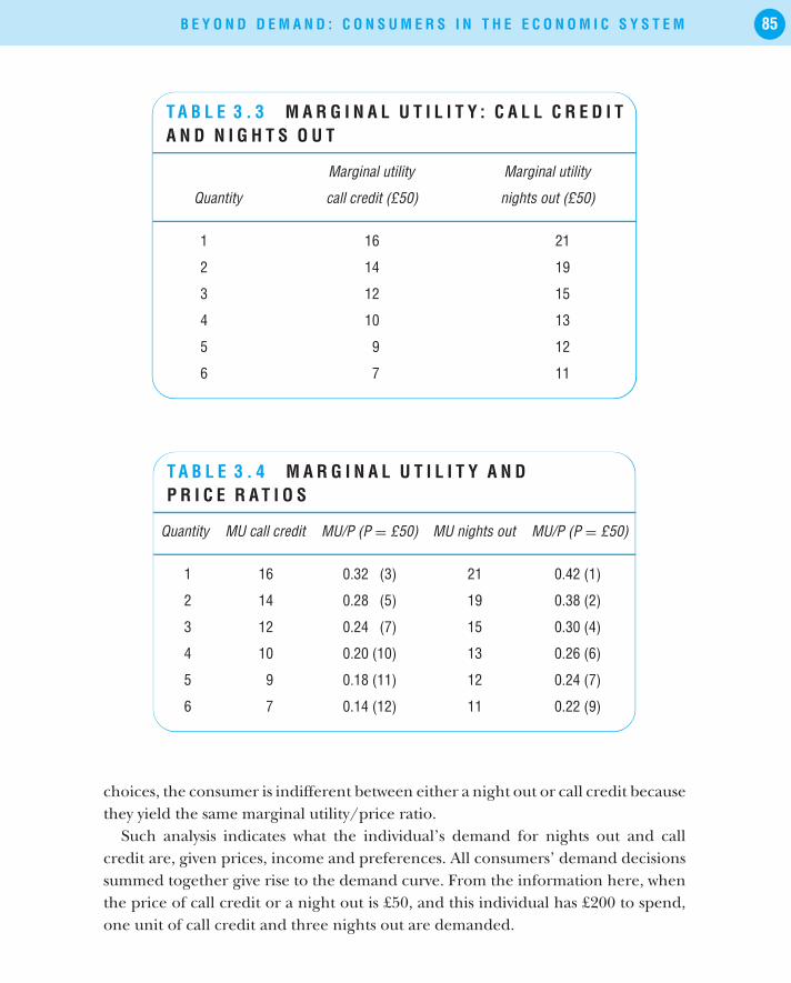
B E Y O N D D E M A N D : C O N S U M E R S I N T H E E C O N O M I C S Y S T E M 85
T A B L E 3 . 3 M A R G I N A L U T I L I T Y : C A L L C R E D I TA N D N I G H T S O U T
Marginal utility Marginal utility
Quantity call credit (£50) nights out (£50)
1 16 21
2 14 19
3 12 15
4 10 13
5 9 12
6 7 11
T A B L E 3 . 4 M A R G I N A L U T I L I T Y A N DP R I C E R A T I O S
Quantity MU call credit MU/P (P = £50) MU nights out MU/P (P = £50)
1 16 0.32 (3) 21 0.42 (1)
2 14 0.28 (5) 19 0.38 (2)
3 12 0.24 (7) 15 0.30 (4)
4 10 0.20 (10) 13 0.26 (6)
5 9 0.18 (11) 12 0.24 (7)
6 7 0.14 (12) 11 0.22 (9)
choices, the consumer is indifferent between either a night out or call credit becausethey yield the same marginal utility/price ratio.
Such analysis indicates what the individual’s demand for nights out and callcredit are, given prices, income and preferences. All consumers’ demand decisionssummed together give rise to the demand curve. From the information here, whenthe price of call credit or a night out is £50, and this individual has £200 to spend,one unit of call credit and three nights out are demanded.
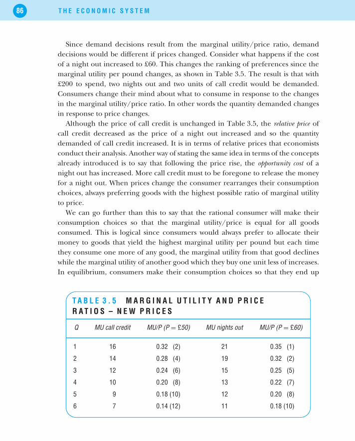
86 T H E E C O N O M I C S Y S T E M
Since demand decisions result from the marginal utility/price ratio, demanddecisions would be different if prices changed. Consider what happens if the costof a night out increased to £60. This changes the ranking of preferences since themarginal utility per pound changes, as shown in Table 3.5. The result is that with£200 to spend, two nights out and two units of call credit would be demanded.Consumers change their mind about what to consume in response to the changesin the marginal utility/price ratio. In other words the quantity demanded changesin response to price changes.
Although the price of call credit is unchanged in Table 3.5, the relative price ofcall credit decreased as the price of a night out increased and so the quantitydemanded of call credit increased. It is in terms of relative prices that economistsconduct their analysis. Another way of stating the same idea in terms of the conceptsalready introduced is to say that following the price rise, the opportunity cost of anight out has increased. More call credit must to be foregone to release the moneyfor a night out. When prices change the consumer rearranges their consumptionchoices, always preferring goods with the highest possible ratio of marginal utilityto price.
We can go further than this to say that the rational consumer will make theirconsumption choices so that the marginal utility/price is equal for all goodsconsumed. This is logical since consumers would always prefer to allocate theirmoney to goods that yield the highest marginal utility per pound but each timethey consume one more of any good, the marginal utility from that good declineswhile the marginal utility of another good which they buy one unit less of increases.In equilibrium, consumers make their consumption choices so that they end up
T A B L E 3 . 5 M A R G I N A L U T I L I T Y A N D P R I C ER A T I O S – N E W P R I C E S
Q MU call credit MU/P (P = £50) MU nights out MU/P (P = £60)
1 16 0.32 (2) 21 0.35 (1)
2 14 0.28 (4) 19 0.32 (2)
3 12 0.24 (6) 15 0.25 (5)
4 10 0.20 (8) 13 0.22 (7)
5 9 0.18 (10) 12 0.20 (8)
6 7 0.14 (12) 11 0.18 (10)

B E Y O N D D E M A N D : C O N S U M E R S I N T H E E C O N O M I C S Y S T E M 87
consuming quantities of goods where the last pound spent on each good yields thesame marginal utility per pound as the last pound spent on every other good. If thiswere not the case total utility could be further maximized of consuming less of onegood and more of another.
3.4.1 THE LAW OF DEMAND – INCOME AND SUBSTITUTIONEFFECTS
The foregoing analysis can be further examined making reference to Income andSubstitution effects, as mentioned in Chapter 2. The income limits facing consumerscan be presented using a graphical tool called the budget constraint, which showsthe different combinations of goods that can be purchased with a set income, givenprevailing prices.
A consumer’s preferences can be illustrated using another graphical tool, theindifference curve, which illustrates various consumption combinations of twogoods, which generate the same utility for a consumer. These tools are presented inFigure 3.2 using the information from Tables 3.3 and 3.4. Since the consumer hasan income of £200 and the prices of credit or a night out are £50, the maximumamount of either good that could be purchased is 4 units, reflected in the budgetline/constraint.
The indifference curve has a curved shape because of the diminishing marginalutility from consuming additional units of each good. The more of one goodbeing consumed, say nights out, the lower the marginal utility from additionalconsumption of that good. If a consumer consumes many nights out, they wouldbe willing to forego a night out for some call credit, and when little call credit is
4Callcredit
Nights out
Budget line/constraintx
4
Indifference curves (IC)
IC1IC2
IC3
1
2
3
1 2 3
F I G U R E 3 . 2 B U D G E T L I N E A N D I N D I F F E R E N C EC U R V E A N A LY S I S

88 T H E E C O N O M I C S Y S T E M
consumed, its marginal utility is high. This is why different combinations of creditand nights out on the indifference curve give rise to the same level of utility.
At different points on the indifference curve, the consumer is willing to tradedifferent amounts of call credit for nights out reflecting the marginal rate ofsubstitution of the goods. This is also reflected in the slope of the indifferencecurve at any point.
Consumers have a set or map of indifference curves, each with the same shape,that reflect their preferences. Each indifference curve refers to one specific level ofutility. On indifference curve IC3 , the consumer has a higher utility level than onIC2 or IC1. Rational consumers attempt to maximize their utility which is equivalentto a desire to consume on the highest possible indifference curve. The actualconsumption decision results from preferences indicated by the set of indifferencecurves and limited income represented by the budget line.
In line with our earlier observation, the consumer in Figure 3.2 chooses toconsume 3 nights out and 1 unit of call credit with income of £200, prices of £50for both goods and given their preferences. Consumption is at point x on IC2 .
The indifference curves drawn for this consumer lie closer to the nights out axisthan the call credit axis, which indicates this consumer’s tastes. Another consumermay prefer fewer nights out relative to call credit (if they are new to an area, havenot yet made too many friends and prefer to chat to friends back home).
The consumer’s demand decision changes with a price change. If the price ofa night out rises to £60, then the maximum number that could be purchasedwith £200 is 3.3 (£200/60 = 3.33). The budget line changes as shown in Figure 3.3and consumption moves from x to y. The steeper slope of the line indicates thatfollowing the price rise, more call credit must be sacrificed, in opportunity costterms, to afford one night out. The consumer’s decision to change their quantitydemanded of both goods can be broken down into a substitution effect and anincome effect.
A price change induces consumers to change their demand decisions. Thesubstitution effect indicates the adjustment in quantity demanded by a consumerdue to the change in relative prices alone.
The income effect reflects the adjustment in quantity demanded due to thechange in real income alone.
The substitution effect can be examined by considering the price effect alone onthe consumer’s choice. To see this we draw a line with the same slope as the new

B E Y O N D D E M A N D : C O N S U M E R S I N T H E E C O N O M I C S Y S T E M 89
4
3
2
1
Credit
Nights out
x
4
IC1 IC2
y
3.33
z
1 2 3
F I G U R E 3 . 3 C O N S U M P T I O N W I T H N E W B U D G E T L I N E
budget line and examine where it intersects the original indifference curve IC2 . InFigure 3.3, this occurs at point z.
The substitution effect is measured from x to z. The change in relative pricesalone leads to a reduction in quantity demanded of nights out but an increase inthe quantity demanded of call credit. The rational consumer substitutes away fromthe relatively more expensive good towards the relatively cheaper good.
The income effect involves examining the effect on quantity demanded of thereduction in real income caused by the price rise in one good holding relative pricesconstant. It is shown by the comparison of point z with point y where the samerelative prices are used, reflected in the same slope of the two lines. Less of bothgoods are consumed at point y on IC1 compared to point z on IC2 . The increasedprice reduces the consumer’s purchasing power and is reflected in reduced demandfor all goods, not simply for the good which has become more expensive. This isthe pure income effect of the price rise for one good, a normal good.
Normal good: one for which demand falls if real income falls or for whichdemand rises if income rises.Inferior good: one for which demand rises if real income falls or for whichdemand falls if real income rises.
Inferior goods are bought when consumers do not have the required purchasingpower to buy other preferred goods. Examples would be many of the goods boughtby low-income households – cheaper cuts of meat, non-brand items, etc. The pureincome effect of a price fall leads to increased purchasing power and an increase indemand for all normal goods, which are most goods.

90 T H E E C O N O M I C S Y S T E M
C O N S U M E R P R E F E R E N C E S
Where do our preferences come from? Parents, school, friends, experi-ence, advertising? Interesting new research has revealed that neuromar-keting – brain scanning via electroencephalogram mapping and functionalmagnetic-resonance imaging – can be used to analyse consumers’ purchasingdecisions and reveal how preferences feed into purchasing decisions.
Neuromarketing is particularly useful for explaining the value of branding.Blind taste tests repeatedly put Pepsi ahead of Coke, which shows up in brainscans that identify greater response of ‘reward centres’ in the brain to Pepsi.Yet Pepsi is not the brand leader. In non-blind taste tests, where subjects weretold which cola they were tasting, Coke won out.
Such consumer behaviour was explained in terms of the strength of itsbrand in the minds of the subjects, which was evident in activity in anotherarea of the brain associated with thinking and judging.
If such thinking and judging activity can be stimulated and influenced byadvertising, for example, companies will be able to shape our preferences moreclearly! Such research is in its infancy but holds interest for anyone interestedin processes that create and change our preferences.
Before we get too carried away with such tests, it has also been pointedout that there is a clear difference between a taste test using a small quan-tity of product and consuming a larger quantity. Specifically in the colaexample, the immediate sugar ‘reward’ from drinking Pepsi is apparentlymuch higher and is preferred in taste tests for this reason. Drinking morethan a taste changes the consumer’s perception and the product is found‘too sweet’ by a majority of the population – no neuromarketing explanationrequired.
3 . 5 D E M A N D , C O N S U M E R SA N D C O N S U M E R S U R P L U S
Since consumer satisfaction is examined by means of utility, it should be possibleto consider the satisfaction of more than one person in isolation. A problem arisesthough because utility is subjective and while it is possible to consider one person’spreferences, by asking them to rank them and try to quantify the satisfactionderived from consumption, it is impossible to sum up the satisfaction of more

B E Y O N D D E M A N D : C O N S U M E R S I N T H E E C O N O M I C S Y S T E M 91
Quantity (000)
Price
50
75
100
D
S
150
18 27 36
F I G U R E 3 . 4 D E M A N D F O R C A L L C R E D I T A N DC O N S U M E R S U R P L U S
than one consumer or try to rank their different preferences. Economists try toget around this problem by means of moving analysis from utility to demand, inthe knowledge that the sum of individuals’ consumption choices (based on theirmarginal utilities) are revealed in the demand for any good. (Economists also usecommunity indifference curves as approximations for the preferences that may begauged for a group of individuals, despite the difficulties involved.)
Consider the demand for call credit shown in Figure 3.4, with supply includedalso. Given demand and supply as shown, the equilibrium in the call credit market isfor 36 000 units at £50 per unit (the single consumer considered in earlier analysis isjust one buyer in the market). The demand at this price is the result of the decisionsof many different individuals based on their derived utility from consuming callcredit, and their marginal utility/price ratios.
The overall satisfaction generated by the equilibrium consumption can beestimated using the concept of consumer surplus.
Consumer surplus – the benefit to consumers due to the difference betweenwhat consumers actually pay to consume a good and what they would have beenwilling to pay.
In Figure 3.4, although the equilibrium price is £50, many people are willing to paya higher price. At a price of £75, 27 000 units are demanded while at a price of£100, 18 000 units are in demand. In fact the area under the demand function andabove the price provides an estimate of the value of satisfaction generated fromconsumption of this product (shown as the shaded triangle). The area of this triangleis computed as £1.8 million (the area of a triangle is half the base × perpendicularheight which here is 18 000 × 100 = 1 800 000). This indicates the estimated valueof the satisfaction generated from the consumption of equilibrium call credit.

92 T H E E C O N O M I C S Y S T E M
3.5.1 CONSUMER SURPLUS AND CONSUMER WELFARE
Welfare economics focuses on assessing the effects of economic policies on bothconsumers and producers. Such assessments depend to a large extent on thevalues (or normative judgements) of the assessors because issues of fairness comeinto play. Issues considered include the conditions under which an economyis most efficient and how goods and income are distributed within economies,and how different economic policies impact on stakeholders. The effect of aneconomic policy on consumers can be investigated by looking at changes toconsumer surplus.
For example, if a government ensures that there is additional competition in thetaxi market (by allowing extra taxis to be registered), this could lead to an increasedsupply of taxis. This is shown in Figure 3.5 as the increase in supply in panel Bcompared to panel A.
The result of expanded supply (from S1 to S2) with the same demand, is alower price for taxi fares with a greater quantity supplied: compare P∗ to P∗∗ andQ ∗ to Q ∗∗. The welfare effects can be considered by examining consumer surplus(CS) in both cases, which is the area above the price and below the demandcurve. At lower taxi fares, in panel B, consumers’ welfare is improved since someconsumers unwilling to pay higher taxi fares become willing to demand taxis andthose who were willing to pay higher prices still benefit given the gap betweenthe price paid and willingness to pay. Consumer welfare can be said to haveincreased since a comparison shows that CS1 in panel A is smaller than CS2 inpanel B.
Q*Q
Quantity Quantity
PS1
D
P*
Q**Q
DP**
S2
Price Price
P S1
A B
CS1CS2
F I G U R E 3 . 5 C O N S U M E R W E L F A R E A N D T H E T A X I M A R K E T

B E Y O N D D E M A N D : C O N S U M E R S I N T H E E C O N O M I C S Y S T E M 93
3 . 6 C O N S U M E R S ’ R E S P O N S E T O P R I C EC H A N G E S
The quantity of goods demanded changes in response to price changes, resultingfrom new marginal utility/price ratios. If the price of all goods fell by 10% consumerswould demand more of most if not all goods, but the rise in demand in responseto the price fall would not be the same across all goods. This is because consumersare more or less price-sensitive for some goods relative to others. No matter whatprice cow’s tongue is I will never choose to increase my demand for it from zero!While individual preferences play a key role in demand decisions and in reactionsto price changes we know they are not the only explanatory factor for consumers’responses to price changes.
A 10% fall in the price of standard pens will not substantially change the quantitydemanded for most people since pens are inexpensive and only a small portionof consumers’ income is spent on them. In the case of goods that are not boughtvery often, and for which the income share is very small, demand is usually notvery price-sensitive. This information is useful in drawing a demand curve becauseit helps us to decide whether the demand curve is relatively steep or flat. For pensthe demand curve will be relatively steep indicating that a change in price has littleimpact on quantity demanded (see panel A in Figure 3.6).
Demand for theatre tickets is somewhat more responsive to changes in price asthey can be relatively expensive and are quite a discretionary purchase. Hence, thedemand curve is relatively flat such as in panel B in Figure 3.6.
The extent to which substitutes are available for a good also impacts on its price-sensitivity. If the price of one brand of pen were to fall by 10%, rational consumers
Price
Quantity QuantityD
Price
D
P1
P2
P1
P2
A: Pens B: Theatre tickets
Q1 Q2 Q1 Q2
F I G U R E 3 . 6 P R I C E S E N S I T I V I T Y A N D D E M A N D

94 T H E E C O N O M I C S Y S T E M
would substitute away from more expensive pens to the cheaper available brand.For a specific brand, price sensitivity is higher than for a broad category of goods.
In general it is also the case that the higher consumers’ income, the less price-sensitive they are because there are fewer limitations on what can be purchased thanfor people on lower incomes. This means that the demand curves of higher-incomehouseholds would be steeper than for lower-income households and their quantitiesdemanded would change relatively little in response to price changes.
The issue of time is also relevant for analysis of price sensitivity since con-sumers can adjust their purchasing behaviour more easily over longer periods.If one supermarket chain cuts its prices overnight, many people will continueto shop at their usual shops until they become aware of the price cuts else-where and until they are willing and able to change their shopping patterns totake advantage of the cheaper prices (clearly convenience, location and otherfactors matter for the consumer). This may take time but over longer time peri-ods economists expect consumers to be more price-sensitive than over shortertime periods.
F A C T O R S E X P L A I N I N G S E N S I T I V I T Y O F Q U A N T I T YD E M A N D E D T O P R I C E C H A N G E
Ceteris paribus, sensitivity of quantity demanded to price change is low
• for inexpensive goods;
• for goods with a low income share (e.g. clothes pegs);
• for goods in general rather than a specific good, e.g. all pens vs. Paper-mate pens;
• for consumers on high incomes;
• over short relative to longer periods.
3.6.1 PRICE ELASTICITY OF DEMANDIn the taxi example, when supply expanded the result in equilibrium was a lowerprice. As predicted by the law of demand, at a lower equilibrium price consumersdemanded more taxis. The reaction of quantity demanded can be quantified ifinformation is available on the quantities demanded over a range of prices.
The responsiveness of quantity demanded to a change in price is called the priceelasticity of demand (PED).
PED = %�Qd/%�P

B E Y O N D D E M A N D : C O N S U M E R S I N T H E E C O N O M I C S Y S T E M 95
Inelastic: PED < 1
Elastic: PED > 1
Quantity (000)
Price
50
75
100
D
150
125
18 27 36
Price Q (000) PED
125 9 –2.5100
75
50
1827
36
–1.0–0.5
F I G U R E 3 . 7 E L A S T I C I T Y A N D T H E D E M A N D F O RC A L L C R E D I T
If the quantity of taxi rides rose by 10% following a price fall of 5%, price elasticity ofdemand is −2 (%�Qd is 10 and %�P is −5 so PED is −2). Demand elasticities arealways negative numbers but many economists report demand elasticities withoutthe negative sign, assuming that other economists correctly interpret the number.
As the following example shows, information on elasticity is of particular interestto firms in terms of the effects of price changes on their revenues. Returning to thecall credit example, price elasticity can be computed, based on the formula aboveand the information in Figure 3.7.
• Price rise from £50 to £75: PED = 25%/50% = −0.50decline in quantity from 36 to 27 is 9, expressed as a percentage of36 = 25%price rise of £25, expressed as a percentage of £50 = 50%.
• Price rise from £75 to £100: PED = 33%/33% = −1.00decline in quantity from 27 to 18 is 9, expressed as a percentage of27 = 33%price rise of £25, expressed as a percentage of £75 = 33%. Here, thepercentage changes in price and quantity exactly cancel each other out.This is called unit elasticity.
• Price rises from £100 to £125: PED = 50%/20% = −2.50the decline in quantity from 18 to 9 is 9, expressed as a percentage of18 = 50%price rise of £25, expressed as a percentage of £125 = 20%.

96 T H E E C O N O M I C S Y S T E M
PED differs at different points on the demand curve.In absolute terms (ignoring the minus sign) PED is greater than one when the
percentage change in quantity demanded is greater than the percentage changein price. This is elastic PED.
PED is less than one when the percentage change in quantity demanded is lessthan the percentage change in price. This is inelastic PED.
An alternative estimation method may be used. Instead of computing elasticityrelative to one point on the demand function, it can be estimated as an averageover a section of the demand function:
Arc price elasticity of demand:
�Qd�P
× 1/2[P1 + P2]1/2[Qd1 + Qd2]
Arc price elasticity differs to the earlier method by estimating average price andaverage quantity demanded. It is most appropriately used for large price changes.
Re-calculating elasticities from the data above according the arc elasticitymethod reveals:
• Price rise from £50 to £75: Arc PED = − 925
× 1/2[50 + 75]1/2[36 + 27]
= −0.72
• Price rise from £75 to £100; Arc PED = − 925
× 1/2[75 + 100]1/2[27 + 18]
= −1.40
• Price rise from £100 to £120; Arc PED = − 925
× 1/2[100 + 125]1/2[18 + 9]
= −3.00
Price elasticity of demand and total revenue
If a firm wishes to change the price of a good, it can estimate the impact on thequantity demanded of its product by using PED. Staying with Figure 3.7, if the firmis considering an increase in price it can consider the impact on its revenues. Fromconsumers’ perspectives firm revenue is the same as consumers’ expenditure.
A firm’s total revenue is price times the quantity of goods sold: TR = P × Q

B E Y O N D D E M A N D : C O N S U M E R S I N T H E E C O N O M I C S Y S T E M 97
Example: following Figure 3.7
P = £0 Q = 0 TR = £0P = £50 Q = 36 000 TR = £1 800 000 Price ↑ 0–50 TR ↑P = £75 Q = 27 000 TR = £2 025 000 Price ↑ 50–75 TR ↑P = £100 Q = 18 000 TR = £1 800 000 Price ↑ 75–100 TR ↓P = £125 Q = 9 000 TR = £1 125 000 Price ↑ 100–125 TR ↓
Conclusion: increasing price can lead to rises in TR OR to falls in TR .
The relationship between quantity demanded, price, elasticity and total revenue isalso evident from Figure 3.8. In the elastic part of the demand curve, where quantitydemanded is very responsive to changes in price, a fall in price leads to an increasein total revenue.
In the elastic portion of the demand curve, TR changes in the opposite directionto a price change: in the case of a price increase TR falls and in the case of a pricefall TR rises.
In the inelastic portion of the demand curve, TR changes in the same directionas a price change implying that if price increases TR rises also.
Changes in the price of a good almost always result in changes in total revenue. Theexception is at the point on the demand curve where PED = −1 at point c in panel
A
Inelastic:PED < 1
Elastic: PED > 1
Q (000)
Price
50
75
100
D
150
125 Unit elastic:PED = 1
a
b
c
d
TR
1 125 000
2 025 0001 800 000
Q (000)
B
a*b*
c*d*
9 18 27 36 9 18 27 36
F I G U R E 3 . 8 D E M A N D , E L A S T I C I T Y A N D T O T A L R E V E N U E

98 T H E E C O N O M I C S Y S T E M
A when the PED is neither elastic nor inelastic but unit elastic. We saw earlier thatunit elasticity arises when the percentage change in quantity demanded is the exactsame as the percentage change in price so that there is no change in total revenue.
Price elasticity of demand: some special cases
It is possible to envisage situations where irrespective of what price is charged fora product, the quantity demanded would remain constant. Some necessities wouldfall into such categories where irrespective of price consumers have to bear any pricechange. Demand functions for goods to which consumers are addicted might alsodisplay such characteristics. Such a demand function would be a vertical line, shownin Figure 3.9. Since quantity demanded does not react at all to any change in price,it is described as a demand function with perfectly inelastic demand. At a relativelyhigh price of P1 in panel A, the same quantity is demanded as at the lower price ofP2. At the higher price, the firms’ revenue and consumers expenditure is higher.
At the opposite end of the spectrum it is also possible that demand exists for aproduct at only one price, also shown in Figure 3.9. This is possible if we considerthe output of a single firm with many competitors which can only charge the marketprice for their product, i.e. the price determined by market demand and supply (thiscase is considered in more detail later in Chapter 6). Quantity demanded reactsperfectly to any change in price by completely disappearing! The firm can sell asmuch as it wishes to produce at P3 in Panel B of Figure 3.9. If the firm produces Q2it will earn higher revenues than if it chooses to produce Q1.
A Perfectly inelastic demand B Perfectly elastic demand
Price
Quantity Quantity
DP1
P2
Q1 Q1 Q2
Price
DP3
F I G U R E 3 . 9 P R I C E S E N S I T I V I T Y A N D D E M A N D
3.6.2 APPLICATIONS OF ELASTICITY ANALYSISIf a firm seeks to increase its revenue and wishes to change the price it charges fora product, it needs to know to what extent quantity demanded is responsive to theprice change. The above analysis shows that there would be little point in a firm

B E Y O N D D E M A N D : C O N S U M E R S I N T H E E C O N O M I C S Y S T E M 99
raising its price with the intention of boosting its revenues if quantity demandedwas in the elastic part of the demand curve. In terms of a firm’s pricing strategy,therefore, it makes sense for the firm to have information on the price elasticity ofdemand for its product(s).
Information on elasticity is not just of interest to business but can be useful forpolicy-makers also.
If a government is thinking about increasing taxes on cigarettes with theintention of reducing the quantity demanded, it needs to have an estimate ofthe PED for cigarettes.
If the function of the tax is to reduce aggregate expenditure on cigarettes,a price increase (via the tax) would have to result in the price rising tothe elastic portion of the demand curve. The result of the tax would bethat the percentage increase in price would bring about a larger propor-tionally percentage fall in quantity demanded – consumers would buy fewercigarettes, and the total revenue to cigarette firms would decline. Hence,the responsiveness of consumers to price provides useful information fordecision-making.
3.6.3 OTHER ELASTICITY EXAMPLES
Income elasticity of demand
In general if a consumer’s income increases, it is expected that their demand forgoods and services would increase too, but not necessarily by the same proportion.The relationship between the quantity demanded of any goods and income isdescribed by the income elasticity of demand.
Income elasticity of demand measures the responsiveness of the quantitydemanded of a good to changes in consumers’ income (I ).
It is computed as %�Qd/%�Y
Goods are described as normal goods, if their income elasticities are greaterthan zero implying the quantity demanded changes in the same direction as achange in income. Most goods fall into this category – we buy more of them ifour income rises. In the case of inferior goods their quantity demanded declinesif income increases. Income elasticities for inferior goods are negative because apercentage increase (fall) in income leads to a decline (rise) in quantity demandedof the good.

100 T H E E C O N O M I C S Y S T E M
Goods for which the percentage change in quantity demanded is greater than thepercentage change in income are described as income elastic (with income elasticitygreater than one). This would be the case if income rose by 15% and the quantitydemanded of package holidays, for example, increased by 20%. Other goods arecalled price inelastic when a change in income results in a less than proportionatechange in quantity demanded: an example would be a 3% increase in quantitydemanded of electricity following a 15% increase in income. Income elastic goodsare also known as luxury goods whereas income inelastic goods are necessities.
Cross-price elasticity
The relationship between the quantity demanded of one good and the price ofanother good is described by the Cross-price elasticity.
Cross-price elasticity indicates the responsiveness of the quantity demanded ofone good (good A) when the price of another good (good B) changes.
It is computed as %�QdA/%�PB
Cross-price elasticity is of interest for goods that display some economic relationship,such as complement or substitute goods.
If car insurance rises by 20%, this may have an impact on the quantity ofnew cars demanded, a complement good for car insurance, which might beexpected to fall and so the cross-price elasticity would be negative. Since newcars are substantially more expensive than insurance, the effect on demandshould not be close to 20% and so the cross-price elasticity would be lessthan one. Among young drivers and focusing on the first-time drivers’ second-hand car market, the cross-price elasticity might be considerably higher, whenannual insurance costs may even be greater than the price many pay for theirfirst car.
If Indian and Chinese takeaway food are substitute products, it would beexpected that if the price of Chinese takeaways rises, the demand for Indianfood would rise as consumers substitute away from the more expensive to thecheaper good, presuming the consumer is indifferent between the goods. Thismeans that the cross-price elasticity would be positive since the price change(rise or fall) in one good leads to a change in quantity demanded of thesubstitute good in the same direction (rise or fall) as the price change.

B E Y O N D D E M A N D : C O N S U M E R S I N T H E E C O N O M I C S Y S T E M 101
3 . 7 C O N S U M E R C H O I C E A N D P R O D U C TAT T R I B U T E S
Many purchasing decisions are made not between very different products such ascall credit and nights out, but between different brands or types of similar products.Such decisions can be analysed using the attribute model of consumer demand. Thismodel explains that consumer utility, and therefore demand, is the result of productcharacteristics, performance features or attributes, other than price. In selectingone brand of a good over another, consumers compare and subjectively rank theirpreferred attributes, which are those that generate highest utility for them.
The features or attributes that explain consumers’ decisions to buy one varietyor brand instead of another are the basis for product differentiation.
3.7.1 THE ATTRIBUTE MODEL: BREAKFAST CEREALSAn individual considering buying one of the variety of competing cereals has decidedon the two most important non-price attributes for their subjective purchasingdecision as wholegrain cereal and low sugar content. Having evaluated four possibleproducts, the product information is as shown in Table 3.6.
This information is also presented in Figure 3.10 where each of the four productsis drawn as a line against the two attributes and where the slope of each productline reflects the computed ratio of the attributes. The difference in the slopesof the product lines reflects the different trade-offs of the two attributes in the
T A B L E 3 . 6 P R I C E A N D A T T R I B U T EI N F O R M A T I O N F O R B R E A K F A S T C E R E A L S
Attribute rating
(on scale of 1–10 where 1 is lowest) Ratio of
Brand Price Wholegrain Sugar content attributes
A £2.35 9 4 2.25
B £2.59 7 5 1.40
C £2.85 5 7 0.71
D £2.99 3 9 0.33

102 T H E E C O N O M I C S Y S T E M
Wholegrain
Sugarcontent
Brand ABrand B
Brand C
Brand D
A
B
C
D
××
×
×
×
F I G U R E 3 . 1 0 T H E A T T R I B U T E M O D E L
eyes of the consumer (similar to the concept of marginal rate of substitutiondiscussed earlier).
Points A, B, C and D in Figure 3.10 indicate the cost of acquiring each product(which can alternatively be called an attribute combination) as measured from 0 andthe distance reflects the budget the consumer wishes to allot to buying cereal andthe price of each brand. We can simplify having to guess the budget the consumerwants to spend on cereals by assuming our consumer here has sufficient incometo buy any of the four products but their purchasing decision is about buying onepack only (for their weekly shopping). This assumption corresponds more closely tohow purchases actually occur – in terms of one cereal brand versus others. Hence,points A, B, C and D are each one unit out from 0. Points A, B, C and D representthe buyer’s maximum satisfaction/utility frontier and, for example, reflect that atpoint A the attribute combination corresponding to one unit of Cereal A is 9 forwholegrain and 4 for sugar content.
In making the purchasing decision the consumer must evaluate their marginalrate of substitution between the attributes and these are shown by the addition ofindifference curves as in Figure 3.11. The decision of which cereal to purchase isseen from selecting the brand that corresponds to the highest indifference curve,which is Brand B on IC4. The ‘next best’ option is Brand C on IC3, next Brand Aon IC2 and finally Brand D on IC1.
The attribute model can also be used to consider the effect of price changesas this will impact how far on each product line the consumer can purchase andhence a change in price of one brand changes the utility frontier and the highestindifference curve that could be reached. If the price of Brand B increases, for

B E Y O N D D E M A N D : C O N S U M E R S I N T H E E C O N O M I C S Y S T E M 103
Sugarcontent
IC1IC2
IC3IC4
Wholegrain
AB
CD
××
×
×
×
F I G U R E 3 . 1 1 T H E A T T R I B U T E M O D E L W I T HP R E F E R E N C E S
example, then with the same amount of money fewer attributes can be bought(or more must be paid for a given set of attributes). This would have the effect ofmoving the satisfaction frontier reflecting brand B from point B to a point on thesame line but closer to 0. Following the price change, Brand B might no longer bethe consumer’s preferred choice.
3 . 8 A G G R E G AT E C O N S U M E RB E H A V I O U R
Moving from individual microeconomic consumer behaviour to macroeconomicbehaviour we now turn our focus to the general trend that emerges fromanalysing macroeconomic consumption behaviour. The higher people’s dispos-able income – gross income less direct taxes – the more they plan to spend onconsumption goods. If Y denotes income and t denotes the income tax rate, thendisposable income Yd can be defined as Y − tY = Yd. If Y is £30 000 and t is 25%then Yd is £30 000 less £7 500, which is £22 500. The relationship between plannedconsumption expenditure and disposable income for an economy is representedby the consumption function, as shown in Figure 3.12.
Total expenditure on consumption is made up of two components, autonomousconsumption (a) and a fraction of disposable income (b), in other words:
C = a + bYd

104 T H E E C O N O M I C S Y S T E M
Yd
Consumption£bn
50
C = a + bYd(e.g. C = 50 + 0.8 Yd)
a
F I G U R E 3 . 1 2 T H E C O N S U M P T I O N F U N C T I O N
From the consumption function in Figure 3.12, we see that even if disposable incomeis zero, some consumption still occurs. In the figure, this value of autonomousconsumption is £50bn. This is the intercept value of the consumption function.
Consumption expenditure that is independent of the level of income is calledautonomous consumption. It occurs if people borrow to buy consumption goodsor if they spend their savings (or borrow) when they have no income to pay forconsumption goods.
People also spend some of their disposable income. This portion of income isrepresented by b in Figure 3.12 and is the slope of the consumption function.The value of b is different in different countries, and varies over time in countriesalso. It is a fraction lying between 0 and 1. This means that if disposable incomeincreases by £1, for example, planned consumption expenditure will rise but by lessthan £1. Any disposable income not spent on consumption is saved. The term b inFigure 3.12 is known as the marginal propensity to consume – MPC.
The MPC describes the relationship between a change in disposable income andthe resulting change in aggregate consumption expenditure.
As with demand, the ceteris paribus assumption applies to the consumption function.Many factors help to explain the shape of a consumption function for a group ofconsumers. Changes in the factors lead to changes in the consumption function,in either the autonomous component or in the marginal propensity to consume orsometimes in both.
Disposable income is not the only factor that determines consumption behaviour.Other relevant factors include consumers’ wealth, and their expectations aboutfuture prices and income levels. The higher their wealth, whether measured as

B E Y O N D D E M A N D : C O N S U M E R S I N T H E E C O N O M I C S Y S T E M 105
savings, inherited wealth, property or shares, the higher people tend to consumeout of their current disposable income. The rationale is that those with higherwealth have less need to save than other less wealthy consumers. Expectations ofhigher future prices would induce rational consumers to purchase sooner ratherthan later as would the expectation of a higher future level of income.
Income distribution across a population also affects consumption behaviour sincepoorer consumers tend to have a higher MPC and tend not to have the luxuryof being able to save out of their low incomes. Tastes and preferences regardingborrowing and buying on credit also affect consumption and this is true both forindividuals and groups or nationalities.
A consumption function shifts with changes in:
• Wealth: greater wealth → increased consumption (reflected in either higherautonomous consumption or a higher MPC).
• Expectations of future prices and future income: expectations of higher pricesor higher income → increased current relative to future consumption(reflected in either higher autonomous consumption or a higher MPC).The specific effects depend on consumers’ opinions as to how long higherprices will prevail and the expected increase and size of the increasein income.
• Income distribution: the higher the share of rich people in the population thelower the marginal propensity to consume as rich consumers have morediscretion in how to spend income. A rise in the proportion of rich peoplein the population would reduce the MPC and may change autonomousconsumption also.
• Preferences regarding buying on credit: an increase in preferences to borrow forconsumption purposes increases the MPC and may increase autonomousconsumption also.
If the MPC is 0.8 this means that 80p out of every additional £1 is spent onconsumption goods. Furthermore, it implies that the marginal propensity to save isequal to 0.2 and that 20p will be saved out of each £1. A savings function can bedrawn to correspond to the consumption function above as shown in Figure 3.13.
The savings function describes the relationship between income and the desiredlevel of savings. If consumers in Figure 3.13 consume £50bn with an income of 0,they must be borrowing or dis-saving. This is why the savings function in Figure 3.13begins at −£50bn on the savings axis. Since whatever income is not used for con-sumption is saved, the slope of the savings function is (1 – b) which is 0.2 in this case.

106 T H E E C O N O M I C S Y S T E M
S = –a + (1 – b)Yd(e.g. S = –50 + (1 – 0.8) Yd)
Yd
Savings£bn
–50
–a
F I G U R E 3 . 1 3 T H E S A V I N G S F U N C T I O N
The extent of borrowing or dis-saving in an economy is of interest since someeconomists have argued any growth in consumer credit can be beneficial or detri-mental for an economy. The value of economic activity increases when consumersborrow whether it is to buy cars, pay for holidays or whatever the consumption goodspurchased. However, if consumers take on too much debt relative to their income,it is argued that there may come a time when consumers can no longer spend onnew goods and services and focus instead on paying off old debts. Potentially, thatcould slow down economic activity.
Consumers’ demand for credit also has a direct bearing on interest rates. Interestrates are the price of money determined in money markets by demand for moneyand the supply of money (both of which are considered in more detail in Chapter 7).As in any market, if the demand (for borrowed money) exceeds the supply (providedby lenders), prices (interest rates) rise. If demand for credit falls and lenders aretrying to fight for customers, they may offer lower interest rates to attract business.
The paradox of thrift is an example of the fallacy of composition which holdsthat although a certain action might make sense for an individual it does notfollow that the same activity makes sense for an economy overall. Increased savingby an individual consumer provides the consumer with increased opportunitiesfor consumption in the future. It does not follow that an economy benefits fromincreased savings. Why?
An unexpected increase in savings implies decreased consumption expen-diture. Firms will sell less than they planned and require fewer employees toproduce output. Unemployment may rise with the result of lower incomes beingearned at the level of the economy overall. Falling income has a knock-on effect

B E Y O N D D E M A N D : C O N S U M E R S I N T H E E C O N O M I C S Y S T E M 107
of reducing consumption expenditure. If such a scenario unfolds, the paradoxof thrift is observed. Further implications may follow with firms reducing theirplanned investments in line with lower expectations of consumer expenditure sothe process continues on and on until the cycle is ended by changes in behaviouronce again.
3 . 9 G O V E R N M E N T P O L I C I E S –C O N S U M E R F O C U S
Many government policies are microeconomic in focus and attempt to influence thedemand for specific products – such as in the case of cigarettes. Annual governmentbudgets often include increased taxes on alcohol and petrol as governments tryto increase their tax revenues. Following the law of demand, with an increase inthe price of a good, whether caused by an increase in taxes on the goods or anyother factor, the expectation is that quantity demanded will fall. We saw earlierthat the extent to which quantity demanded changes in response to a price changedepends on the price elasticity of demand for the product, which is related to theinitial price and quantity demanded of the good – it may be price elastic, unit elasticor inelastic.
Macroeconomic policies are also used to affect consumer spending at a broaderlevel. Since consumption expenditure is such a substantial share of economicactivity, governments sometimes try to focus policies on increasing consumerdemand. This is particularly relevant before and during recessions when consumerdemand slows down as people put off purchases that are not entirely necessary.During recessions consumer confidence is low and unemployment can be high asfirms lay off workers when their output is not in demand.
One policy that governments use to affect macroeconomic consumptionbehaviour is through the tax system. During recessions governments often cutincome taxes so that consumers have more disposable income that they can spendon consumer goods. This is one example of how government attempts to affect theconsumption function. By cutting taxes, consumers have more disposable income,and hence their consumption expenditures would probably rise. Any change in thetax rate alters consumption behaviour via the consumption function, as explainedin this worked example.

108 T H E E C O N O M I C S Y S T E M
T H E TA X R AT E A N D C O N S U M P T I O N
Consider the following consumption function: C = 50 + 0.8YdIf the net tax rate is 20%, this means disposable income is 80% of national
income or
Yd = 1 − 0.2Y = 0.8Y
A change in the net tax rate to 30% would affect consumption behaviour bychanging the amount of disposable income to
Yd = 1 − 0.3Y = 0.7Y
This indicates that when the net tax rate changes consumption is affected.If the change in disposable income had no effect on autonomous consumptionor the marginal propensity to consume then the function itself would remain at
C = 50 + 0.8Yd
However, the impact of having lower disposable income would imply lowerplanned consumption by consumers. If consumers reacted to higher taxes bysaving less, the MPC could increase. The change in tax rate would probablyhave no impact on autonomous consumption.
Alternatively, governments trying to slow down activity in a booming economy mightattempt to make savings a more attractive option.
Special savings accounts might be introduced such as in the case of the IrishSpecial Savings Investment Accounts (announced in the Finance Act 2001). Inthis case the Irish Government provided an additional 25% on each ¤1 savedin these special accounts (minimum monthly savings were ¤12.70: maximumwere ¤254), which would be valid for a five-year period. To qualify for suchattractive returns, savings could not be withdrawn before the five-year periodor taxes equivalent to the government’s contribution would have to be paid.Approximately 40% of the adult population opened such accounts, whichshould mature for withdrawals around the time of the next General Election,should the government serve its full office.
Another government policy that focuses on trying to influence aggregate consump-tion is the expansion of public sector employment, which includes teachers, police,

B E Y O N D D E M A N D : C O N S U M E R S I N T H E E C O N O M I C S Y S T E M 109
civil servants, nurses, doctors, etc. By increasing employment in this way fewer peopleare unemployed and the wages and salaries of the public sector workers can be spenton consumer goods, boosting demand. Unfortunately there are some examples ofcases where governments created additional public sector jobs, which althoughresulting in generating extra consumer demand in the short term also created long-term problems of inefficiency in certain parts of the public sector and increasedgovernment expenditure via wages and salaries (see Johnson and Scholes, 2001).
Other less direct policies are also used by governments to stimulate consumerdemand – as in the car industry example in the Philippines (outlined in Chapter 2).Because a price ceiling was set, consumer demand for a certain type of utility vehiclewas boosted; however, since demand outstripped supply, many consumers willingand able to make their purchase were unable to do so due to the limited supply.This is interesting since it shows how government policies do not always have thedesired effects.
Governments also try to affect consumer behaviour by policies such as banningsmoking in the workplace, as in Norway, New York and Ireland. This means suchgovernments have decided that the social costs of smoking outweigh the benefits toconsumers who wish to smoke. Many debates rage regarding the right of governmentto affect consumption behaviour so drastically and point to the tension betweenprotecting the public on the one hand and impinging on individual freedom froma ‘nanny’ state, on the other.
3 . 1 0 S U M M A R Y
• Expenditure on consumption goods is a substantial component of economic activity.
• Consumption activity can be analysed from a number of perspectives – how individualrational consumers make their consumption decisions, how this is reflected in thedemand for a product in a specific market and how this relates to aggregateconsumption.
• Concepts that allow us to understand the choices consumers make include totalutility, marginal utility and consumer preferences. Price changes impact on plannedconsumption expenditure, i.e. on quantity demanded, which can be analysed usingthe marginal utility/price ratio or using budget line and indifference curve analysis.
• Consumer welfare can be analysed using the concept of consumer surplus.
• Economic decision-making regarding consumer behaviour can be supported byanalysis of price elasticity.

110 T H E E C O N O M I C S Y S T E M
• The attribute model allows for analysis of demand for differentiated con-sumer products.
• Aggregate consumption behaviour is described by the consumption function.
• Government can influence aggregate consumption and/or demand for individ-ual products.
R E V I E W P R O B L E M S A N D Q U E S T I O N S1. Using the information provided, fill in column 3 by computing the marginal
utility of car and motorbike consumption.
Marginal MarginalNo. of Total utility utility No. of Total utility utility
cars (Q) (TU) (�TU/�Q) bikes (Q) (TU) (�TU/�Q)
0 0 – 0 0 –1 50 1 202 88 2 153 115 3 114 135 4 75 150 5 36 162 6 0
2. If the consumer in question 1 had £60 000 to spend and a car or bike cost£15 000:a. Compute the marginal utility per pound for car and bike consumption.b. Rank the consumer’s preferred consumption choices.c. What difference does it make to your answers to (a) and (b) if the price of
the bike is £10 000?3. Given the following information on demand for roses in a small town:
Equilibrium price £10.00Quantity demanded when price is zero 480Quantity demanded when price is £20.00 0
a. Estimate the consumer surplus.b. If there is a change in the supply of roses that leads to an increase in
the equilibrium price to £12.00, estimate the change in consumer surplus.Answer this question by drawing supply and demand curves. Can you thinkof any reasons that might cause supply to change?

B E Y O N D D E M A N D : C O N S U M E R S I N T H E E C O N O M I C S Y S T E M 111
4. List five products that you consume and explain why you are/are not price-sensitive in the case of each one. Which products do you think have the steepestand flattest demand curves? Why?
5. Using the given information, consider if Fair Furniture Ltd should or shouldnot increase its price of tables (hint: compute the total revenue).
Current price £275Quantity sold 500Proposed price £325Expected sales at price = £325 480
In increasing price from £275 to £325, does this correspond to the elastic orinelastic portion of the demand for tables? Explain your answer.
6. For an economy with a consumption function of C = 50 + 0.8Y and a tax rateof 0.2 (or 20%)a. Rewrite the consumption function in terms of disposable income rather
than national income.b. Sketch both consumption functions to consider the effect of taking account
of taxation.c. If the tax rate rises to 0.4, what effect does this have on the consump-
tion function?7. What other products, apart from breakfast cereal, could be analysed using
the attribute model? For one of the products you selected, ask two friends toindicate the most important attributes they consider in purchasing the product.Ask each of them to rank their preferences for each attribute (on a scale of1–10) for four alternative products. Construct a table like Table 3.6 and drawa figure like Figure 3.10 showing the relative performance of the products interms of their attribute ratings.
8. Read the following brief case study and answer the questions that follow.
The European car industry: consumers being taken for a ride?
The price of cars across the EU varies considerably for some makes and models.Many consumer groups have voiced concern over this issue and campaign forreform in this market that will result in greater standardization of prices. Despitethe introduction of the euro, price divergences were still widespread in 2002,although recent information points to some convergence of prices within theeuro zone.
An examination of manufacturers’ recommended retail (pre-tax) pricesshowed considerable diversity between the cheapest and most expensive coun-tries in the euro zone with the average difference being approximately 10%

112 T H E E C O N O M I C S Y S T E M
in November 2002, down slightly on the previous estimate of May 2002. Theeuro zone countries where cars are cheapest are Denmark, Greece and theNetherlands while the most expensive are Germany and Austria. The mostexpensive EU country is still the UK.
For individual cases, some very wide price differences have been recorded,the greatest being for the Fiat Seicento, which costs 59.5% more in the UK thanin its cheapest source, Spain.
In theory, at least, it should be possible for a European consumer to source a carfrom a cheaper location. However, in practice the process is not straightforward.For reports on car price differentials across the EU visit:http://europa.eu.int/comm/competition/car sector/price diffs/a. Would you expect that manufacturers’ recommended retail (pre-tax) prices
would differ for consumers in different countries? Why or why not?b. Why might the introduction of the euro have been expected to reduce any
price discrepancies across the euro zone?c. What obstacles might stand in the way of a consumer wishing to purchase a
car from another country?
F U R T H E R R E A D I N G A N D R E S E A R C H• For more on Simon’s concept of bounded rationality see Simon, 1957.
• Interesting recent research on the implications for economics of research intohuman behaviour was published in Kopcke, Sneddon Little and Tootell, 2004.
• For related reading see Jensen and Meckling, 1994.
R E F E R E N C E SHeston, A., R. Summers and B. Aten (2002) Penn World Table Version 6.1. Centre for
International Comparisons at the University of Pennsylvania (CICUP), October.Jensen, M. and W. Meckling (1994) ‘The nature of man’, Journal of Applied Corporate
Finance, Summer, 4–19.Johnson, G. and K. Scholes (2001) Exploring Public Sector Strategy. Prentice Hall.Kopcke, R., J. Sneddon Little and G. Tootell (2004) ‘How humans behave: impli-
cations for economics and economic policy’, New England Economic Review, FirstQuarter, 1–35.
Simon, H. (1957) ‘A behavioral model of rational choice’, in Models of Man. JohnWiley & Sons, Inc., New York.

C H A P T E R 4
B E Y O N D S U P P L Y : F I R M SI N T H E E C O N O M I C S Y S T E M
�
�
�
�
L E A R N I N G O U T C O M E SBy the end of this chapter you should be able to:
✪ Describe the main activities of firms in the economic system.✪ Clarify why firms are necessary within the economic system.✪ Compare and contrast accounting and economic definitions of profit.✪ Use marginal analysis to consider efficient production for a firm taking its costs
and revenues into account.✪ Explain how producer surplus is a measure of producer welfare.✪ Apply the concept of price elasticity of supply and explain how it is useful for
economic decision-making.✪ Outline the reasons why firms invest and how investment contributes to
economic growth.✪ Apply the demand/supply model to discuss how government tries to influence
producers with specific reference to:
• production subsidies;
• environmental taxes.
4 . 1 I N T R O D U C T I O NJust as the economic system relies on consumers for its existence, suppliers playan equally important role in the organization and functioning of an economy.Suppliers facilitate the exchange of goods and services, which is a cornerstone ofthe economic process. But to see their function as simple intermediaries betweenpeople and goods and services would miss the variety of contributions made by firmsto the continuation, growth and expansion of the economic system. In section 4.2,these contributions are discussed. The reasons why firms exist at all are presentedin section 4.3 and the basic building blocks for microeconomic analysis of firmsare presented in detail throughout this section, i.e. output, revenue and costs. This

114 T H E E C O N O M I C S Y S T E M
analysis is developed further to examine the concept of efficient production froma single firm’s perspective in section 4.4 in the context of a profit-maximizing firm.Efficient production in the face of a lower cost competitor is also considered hereand the extent to which the production decision differs for firms in the short runor long run is examined.
Producers’ welfare is analysed in section 4.5 by estimating producer surplus andthis is followed by consideration of how producers react to changes in prices insection 4.6. The discussion turns to focus on aggregate macroeconomic investmentbehaviour by firms in section 4.7, since the investment function fulfilled by busi-nesses is a vital contribution by firms to the economic system. The role played bygovernment in attempting to influence production is dealt with in section 4.8 wherethe examples of using subsidies and environmental taxes are analysed.
4 . 2 F I R M S I N E C O N O M I C A C T I O NProducers make and supply products and/or services to consumers. Most firmsoperate in the private sector which means those companies are owned and operatedby private individuals. Firms owned and/or operated by governments make up thepublic sector. Firms contribute to economic life in many ways through:
• the goods and/or services they provide;
• the employment they offer;
• the wages and salaries they pay employees;
• the money they spend on buying goods and services from other firms;
• the money they spend on improvements to their businesses (to buy new premisesor new machinery and equipment, for example);
• the taxes they pay for their employees and on their profits;
• their expenditure on innovation to advance and increase the quantity or qualityof products/services they provide.
As we saw in Chapter 3 the consumption behaviour of consumers provides firmswith revenue so in terms of attempting to approximate the contribution of firms toeconomic life, this provides some information. If we consider the overall amountof economic activity conducted in an economy (whether measured as income oroutput) we note that firms also contribute to each of the other components ofactivity by:

B E Y O N D S U P P LY : F I R M S I N T H E E C O N O M I C S Y S T E M 115
• providing some of the goods and services that are provided to government andwhich appear under government expenditure;
• supplying goods and services for exports and by importing such goods also,appearing under net exports;
• their attempts to maintain and improve the level of capital stock of theircompanies, and thereby the economy, classified as investment.
The monetary value of firms’ involvement in economic activity in no way exhaustsall the ways in which firms contribute to economic life. Indeed it would be difficult,if not impossible, to put a value on the utility that individual entrepreneursderive from setting up and running their own businesses rather than working forother employers.
4 . 3 W H Y O R G A N I Z E A N E C O N O M I CS Y S T E M A R O U N D F I R M S ?
As outlined in Chapter 2, hypothetically speaking, economic life does not needto include firms. However, it does make better sense for firms to organize someeconomic activities because it is a more efficient way to use economic resourcesthan if individuals instead engaged in those same activities. Hence, one reason whyfirms are needed is to save on unnecessary transactions costs that would arise ifeconomic activity were conducted by individuals, instead of by firms.
If you were to ask those people actually running firms, the chief executiveofficers or managing directors, why their firms exist, they probably would notexplain that it is to help society save on transactions costs. Similarly, althoughsociety benefits from firms’ advances to create new and innovative products,most firms would probably not rate society’s benefit as their reason for existing.Firms exist rather to generate income for their owners or shareholders and suchincome is generated as long as the firm’s total costs (in the economic sense)are less than its total revenues. This excess of revenue over costs amounts to afirm’s economic profits. Economists generally assume that firms exist to generatethe maximum possible economic profit they can. This is the principle of profitmaximization. This means firms make their decisions about how much to produceand what price they should charge with the aim of making the largest economicprofit possible.

116 T H E E C O N O M I C S Y S T E M
4.3.1 DECISIONS OF FIRMS AND THE ROLE OF TIMEEconomists constantly use the terms short run and long run and the distinction isparticularly relevant when considering the decisions taken by firms. The short runand long run are not just set periods of time and are firm- and industry-specific.
The short run describes the period of time it takes for a firm to change its scale ofproduction and this depends on its fixed factor of production – usually capital.
In the short run a firm has one or more fixed factors of production, which constrainsits possible output.
An ice-cream seller who travels around in his van selling ice-cream conescannot sell more than his machine, van and supplies can produce unless hedecides to put another van on the road. This would take some time dependingon his finances and the ease of finding a suitable van, equipment and driverbut could possibly be done quite quickly so the short run would be quite short,i.e. the time to get another van up and running.
On the other hand for a ship-building company the short run would be muchlonger. A significant amount of equipment and machinery is required to buildships and it could take a long time to build new hangars, buy the necessaryequipment and find the skilled labour if a ship-builder decided to expand itsscale of production. The short run in that case could run into several years.
Usually we consider capital to be the fixed factor in the short run. When economistsconduct analysis in the short run it is also assumed that there are a fixed number offirms in an industry, there is no entry of new firms or exit of existing firms.
The expressions short-term, medium-term and long-term are also commonlyused in economic forecasting and refer to time-periods of up to three years, threeto five years and five years plus respectively.
The long run – when a firm’s output is not limited by fixed factors of produc-tion – the amount of any factor of production can be changed and firms canenter or leave an industry.
Essentially the distinction between short run and long run is useful for dealing withday-to-day decisions a firm takes, i.e. short-run decisions – and more long-term or

B E Y O N D S U P P LY : F I R M S I N T H E E C O N O M I C S Y S T E M 117
strategic issues the firm has to deal with, i.e. long-run decisions. The distinction isuseful in the context of how theory is applied in economics because it provides aframework for focusing on a more constrained set of decisions in short-run analysiswhich can be extended as required to focus on long-run issues.
In considering how firms try to maximize their profits the sections that followhighlight relevant issues for firms separately for the short and long run. Thisrequires consideration of the revenue and costs of a firm. Decision-making basedon economics – such as the decision to produce the quantity of output that allowsa firm to maximize its profits – uses marginal analysis and this is why not onlytotal revenues and costs but also marginal revenues and costs are examined in thesections that follow.
Marginal analysis is the process of considering the effect of small changes in onefactor relevant to an economic decision (e.g. on output levels or pricing) andidentifying whether an economic objective will be met. The objective may relateto profit maximization, benefit maximization, cost minimization or revenuemaximization as examples.
The logic of marginal analysis is that a small incremental change shouldbe made once an economic objective is met – there is economic rationale toincreasing price only if profits rise, if that is the economic objective. If no changeenhances the economic objective (if it is already maximized/minimized) thedecision variable should be changed no further.
Marginal analysis a method for optimizing decision-making within a reasonablywell-defined setting.
4.3.2 FIRM REVENUEThe general pattern followed by the total revenue of a firm with a ‘standard’ lineardownward sloping demand function was presented in Chapter 3 and is repeatedhere in Figure 4.1. Total revenue received by a firm is calculated as price × quantity(in equilibrium) so if price is £20 and quantity sold is 50, total revenue is £1,000.Depending on the amount of output the firm sells its total revenue varies. Sincequantity demanded varies with price (higher price corresponding to lower quantitydemanded and vice versa), then the price the firm charges has a bearing on itsrevenues. A firm’s demand curve provides the information needed to sketch itstotal revenue curve.
Consider the total revenue curve in panel A of Figure 4.1. We refer to the callcredit example used in earlier chapters except here we deal with one firm supplyingsome of this market. If the firm charges a price of £150, consumers are not willing to

118 T H E E C O N O M I C S Y S T E M
Q (00)
MR
Rev
TR
112 500
202 500180 000
Q (00)
b*
c*d*
TR19 18 27 36 9 18 27 36
A B
a*
F I G U R E 4 . 1 T O T A L R E V E N U E A N D M A R G I N A L R E V E N U E
buy its product and no revenue is earned (shown as TR1 in the bottom left cornerof Figure 4.1) At a price of £125 the firm would sell 900 units and earn revenueof £112 500 (see a∗). If price is relatively lower at £100, more consumers buy theproduct and 1800 units are sold. Hence, total revenue rises to £180 000 (see b∗). Ifprice is cut further to £75, more consumers are enticed to buy the product, 2700units are sold and total revenue rises further to £202 500 (see c∗). Two effects areassociated with the quantity increase from 1800 to 2700 for example. On the onehand there is a negative impact on firm revenue since the price has dropped from£100 to £75. However, the effect of increasing quantity demanded more than offsetsthe price effect and so total revenue rises.
Any further cuts in price still increase the quantity sold (e.g. 3600, etc.) but theextra sales at the lower price required to entice more consumers to make their pur-chase result in lower total revenue for the firm; the effect of the price reduction off-sets the rise in sales. The firm maximizes its total revenue if it sells the quantity 2700but this amount of output can only be sold if the firm chooses the ‘correct’ price.
If revenue maximization is the firm’s objective it needs to consider what demandfor its product is in order to set the required price to sell the optimal amount ofoutput. In panel B of Figure 4.1 marginal revenue (MR) is graphed.
Marginal revenue is defined as the change in total revenue associated with achange in quantity demanded.
The marginal revenue function shows the amount of additional revenuegenerated for a firm at different levels of quantity demanded. It is computedas the change in total revenue divided by the change in quantity demanded:�TR/�Q .

B E Y O N D S U P P LY : F I R M S I N T H E E C O N O M I C S Y S T E M 119
To understand the linear MR curve, take the example of a firm that setsa high price for its product (say £800 for a wooden table) so that quantitydemanded is just one unit. The firm earns total revenue of the price of thetable × 1 unit = £800.
If the firm drops its price to £725, it could sell two tables. If it did so it wouldearn total revenue of £725 × 2 = £1450. Since total revenue changes whendifferent prices are charged, so too does marginal revenue.
The change in total revenue when two tables are sold compared to whenone was sold is £1450 – £800 = £650.
Therefore, the marginal revenue for the first table sold is £800 while themarginal revenue for the second table is £650. To sell additional tables thefirm would have to cut its price further so that the marginal revenue declinesfurther as quantity demanded and sold rises.
Focusing on Figure 4.1 marginal revenue can be computed as:
Total MRPrice Quantity revenue �TR �Q �TR/�Q
£150 0 0 0 0 0£125 900 £112 500 £112 500 900 £125£100 1800 £180 000 £67 500 900 £77.20£75 2700 £202 500 £22 500 900 £25£50 3600 £180 000 −£22 500 900 −£25
Conclusion: marginal revenue declines as quantity demanded rises. Firmsmust lower price to increase quantity demanded and this impacts on totalrevenue and on marginal revenue.
In Figure 4.1 panel A, total revenue rises up until its maximum at 2700, after whichit drops. This means that a small, marginal increase in output from 2699 to 2700corresponds to the change in output where the effects on total revenue of thedrop in the price and increase in quantity of output exactly cancel each other out.Beyond quantity demanded of 2700 any change in total revenue is a decline andthis is reflected in the MR function, which dips below 0 beyond this level of output.

120 T H E E C O N O M I C S Y S T E M
The effect of the price reduction beyond £75 has a greater negative effect on totalrevenue than the effect of increasing quantity demanded.
Firm revenue is just one component in the profit-maximizing decision of thefirm. The next relevant component is output.
4.3.3 FIRM OUTPUT (PRODUCT): MARGINAL AND AVERAGEOUTPUT
What a firm can produce depends on the inputs available to it, both in terms ofthe quantity and quality of those inputs. At its simplest, what comes out of a firmdepends on what goes in. The exact relationship between inputs and output will bedifferent for each firm since different firms are in different lines of business andwill have very different input requirements, different resources, both capital andhuman. Even for firms within the same industry or line of business, the relationshipbetween inputs and outputs will vary as firms will have different inputs available tothem and different strengths and weaknesses in successfully converting their inputsinto output. A general relationship between inputs and output, however, can begraphed, as shown in Figure 4.2.
Putting one input (labour) on one axis, total output, also referred to as total prod-uct, can be drawn. If we consider the output of a firm in the short run, we assume thatits capital input is fixed while its labour input can be varied. This is the simplest casethat we can use to display the relationship between output and factors of production.
The S-shape of the total product curve represents the general relationshipbetween variable input(s) and output for any firm, where L1, L2 and L3 representdifferent numbers of workers. In the short run, the more workers a firm employs,the higher its total output up to a point. Beyond that point (C), additional workersjust get in each other’s way and total output begins to fall.
Output
LabourL1 L2 L3
Total product curve
A
BC
Q2
F I G U R E 4 . 2 T O T A L O U T P U T ( P R O D U C T )

B E Y O N D S U P P LY : F I R M S I N T H E E C O N O M I C S Y S T E M 121
The relationship between output and labour input is not a simple linear relation-ship, as the S-shape indicates. Up to a certain number of workers – L1 – total outputrises more and more with each additional worker. This is reflected in an increase inthe slope of the total output curve up to point A in Figure 4.2. This is the portion ofthe total product curve that reflects increasing marginal physical product of labour(the MPPL was discussed in Chapter 2).
Marginal physical product of labour: the change in the quantity of outputproduced by each additional worker: �Q/�L.
When L1 workers are employed, MPPL is at its maximum, as seen in Figure 4.3.After point A, the MPPL declines implying that although total output still increasesas the quantity of workers increases, its rate of increase slows down. This is reflectedin a decrease or flattening of the slope of the total output curve beyond point A inFigure 4.2.
The pattern in the average product of labour can also be considered withreference to Figures 4.2 and 4.3.
Average product of labour: total output divided by the number of workers: Q/L.
For example, with L2 workers, the firm shown in Figure 4.2 produces Q2 out-put – at point B on the total product curve. If this output corresponds to 200 tables,produced by 160 workers, each worker produces 1.25 tables on average. For allvalues of total output below Q2 (and the corresponding number of workers belowL2) the average product of labour is less than at point B. For example, at L1 120workers produce 140 tables, a lower average of 1.2 tables each. For all values oftotal output above Q2, and the corresponding number of workers above L2, average
Output
Labour
Average product
Marginal product
a
b
c
L1 L2 L3
F I G U R E 4 . 3 M A R G I N A L A N D A V E R A G E O U T P U T( P R O D U C T ) O F L A B O U R

122 T H E E C O N O M I C S Y S T E M
product of labour is lower than at point B. (At any point apart from B on the totalproduct/output curve, the slope of a line drawn between zero and that point onthe total product curve is lower than at point B. The slope expresses the verticaldistance between zero and the output quantity relative to the horizontal distancebetween zero and the quantity of labour, i.e. the measure of average output perworker: Q/L.) At L3 with 260 workers, output is 240 tables, or 0.92 of a table.
This explains why in Figure 4.3, point b is the highest point on the averageproduct of labour curve. From this figure we see that:
• When the marginal physical product of labour lies above the average productof labour, hiring one extra worker leads to an increase in the average productof labour.
• When the marginal physical product of labour lies below the average product oflabour, hiring one extra worker leads to a fall in the average product of labour.
• The marginal physical product of labour curve intersects the average productof labour curve from above at the highest point on the average product oflabour curve.
The shape of the marginal product curve can be understood from the analysis ofthe labour market and the discussion of the law of diminishing marginal returnsdiscussed in Chapter 2.
M A R G I N A L A N D A V E R A G E R E L AT I O N S H I P S
Linda is taking a course with five continuous assessment exercises, eachcounting for 20% of the overall course mark. Linda would like to do well in allexams but her key objective is to score 50% overall so she can pass the courseand move on to the next year of her studies.
Linda scores as follows in the exams:
Exams #1: 60% #2: 65% #3: 52% #4: 60% #5: 64%
Total marks: 60 125 177 237 301
Linda’s average mark after the first exam was 60%.Her average mark over the first two exams is [60 + 65]/2 = 62.5%.Her average mark over the first three exams is [60 + 65 + 52]/3 = 59.0%.Her average mark over the first four exams is [60 + 65 + 52 + 60]/4 = 59.25%.Her average mark over the five exams is [60 + 65 + 52 + 60 + 64]/5 = 60.2%.

B E Y O N D S U P P LY : F I R M S I N T H E E C O N O M I C S Y S T E M 123
The marks received in each exam correspond to the definition of marginalmarks – the change in total marks for each extra exam completed: the changein marks after the second exam is the total marks 125 minus the marks for thefirst exam or 125 − 60 = 65.You can see that:
• When the marginal mark rose (eg. 60% to 65%), the average also rose(from 60% to 62.5%).
• When the marginal mark fell (eg. 65% to 52%), the average also fell (from62.5% to 59%).
• When the marginal mark was greater than the average, the averageincreased (look at exams #1 and #2).
• When the marginal mark was less than the average, the average declined(consider exams #2 and #3).
4.3.4 FIRM COSTSFirms must pay a range of different costs, depending on their circumstances andline of business – costs for rent, rates, insurance, taxes, wages, salaries, productioninputs, machinery, computers, refuse collection, accountants’ fees, etc. A firm’stotal costs are the sum of variable and fixed costs.
Total costs (TC) are the sum of variable costs and fixed costs.Variable costs (VC) or total variable costs (TVC) depend directly on the amountof output the firm produces, such as the costs for production inputs and workers.The higher the quantity produced the higher the variable costs.
Other costs such as rent and rates must be paid even if the firm produces nooutput and these costs are called fixed costs (FC) or total fixed costs (TFC).
TC = TVC + TFC
Total fixed costs can be graphed easily, as shown in Figure 4.4, since they do notchange as output changes. If when adding up all a firm’s fixed costs, total fixedcosts are £2750 per week, then these costs must be paid by the firm if output is zeroor not.
In panel B of the figure, average fixed costs are shown. The average fixed cost ofthe first unit of output is £2750/1 = £2750; for the second unit it is £2750/2 = £1375;

124 T H E E C O N O M I C S Y S T E M
Costs
Output
TFCFC = £2 750
1000 3000Output
Costs
AFC
1000 3000
A B
F I G U R E 4 . 4 T O T A L F I X E D C O S T S ( T F C ) A N D A V E R A G EF I X E D C O S T S ( A F C )
for the third unit it is £917 and so on, so the more the firm produces the lowerits average fixed cost as the fixed costs can be spread across a greater amount ofoutput. The average fixed costs of 1000 units of output would be £27.5 while theaverage fixed cost for 3000 units would be £0.92.
Variable costs change with output, which was shown above as total output. Thetotal variable costs curve for any firm follows an inverted S-shape since it is relatedto the total output curve. It is drawn based on available information on the priceof inputs and knowledge about the best available techniques (technology) forconverting inputs into output. In short-run analysis, technology is assumed to befixed so the cost curves are drawn assuming a certain level of technology.
The best technique for transforming inputs into output can depend on theamount of output produced. It may make sense for a large car producer to invest inrobotic technology because of the quantity produced but this technology would betoo expensive and make no economic sense for a small-scale car producer. Largedairy companies use large container vats for cheese-making; such investment inequipment would be unsuitable and too expensive for smaller homemade cheeseproducers.
The general shape of any firm’s total variable cost curve (TVC) is shown inFigure 4.5. The first units of output generate high initial costs for a firm – the firstworker is hired, initial inputs must be bought (often in bulk) and the most efficientways to produce output are yet to be learned by the workforce – often it is only fromworking on-the-job (learning by doing) that the best ways to produce efficientlyare understood and put into practice. Hence, in the initial stages of production,until point a on the TVC curve, total costs rise proportionately faster than output.Once efficiencies are realized, production costs still increase but not as quickly asoutput. Beyond point b, there is no point in producing extra output as costs risesignificantly faster than output.

B E Y O N D S U P P LY : F I R M S I N T H E E C O N O M I C S Y S T E M 125
TC
Cost
Output
TVCCost
Output
A
B
FC
a
b
A B
F I G U R E 4 . 5 T O T A L V A R I A B L E C O S T ( T V C ) A N D T O T A LC O S T ( T C )
A firm’s total costs are found by adding up its total fixed and total variablecosts. Graphically this gives rise to a figure similar to Figure 4.5 panel A, the onlydifference being it does not start at zero cost when output is zero since fixed costs(FC) must be paid. This is shown in Figure 4.5 panel B, which differs from panel Aonly with respect to fixed costs that have been added on at each point on the totalcost curve.
4.3.5 MARGINAL AND AVERAGE COSTSThe marginal and average cost curves that correspond to the total cost curve isshown in Figure 4.6.
Average cost (AC) is total cost per unit of output. AC is computed as total costsdivided by output (TC/Q).
Average total cost (ATC) is made up of average variable cost (AVC) plusaverage fixed cost (AFC): ATC = AVC + AFC.Marginal cost (MC): the change in total costs as output changes (�TC/�Q).
Firms’ average cost (AC) curves tend to follow a general U-shaped pattern. TheAC curve for a firm with relatively low costs would lie below the AC curve for ahigher-cost firm.
The minimum point on a firm’s AC curve corresponds to the level of output thefirm should produce in order to produce at its minimum average cost. However,an individual firm cannot always sell this amount of output – there may not be amarket for it. Producing at minimum average cost would be a welcome outcomefrom the perspective of making efficient use of economic resources but firms do

126 T H E E C O N O M I C S Y S T E M
Cost
OutputQ1
AC
MCC
Q2 Q3
AB
F I G U R E 4 . 6 M A R G I N A L C O S T ( M C ) A N D A V E R A G EC O S T ( A C )Notes: If TVC = ¤2500 when 250 units are sold, AVC = ¤2500/250 = ¤10.If TVC rise to ¤3000 when 275 units are sold, the MVC of the additional 25 units of output is ¤500 intotal or ¤12 per unit.
not always produce this amount of output as it does not always coincide either withdemand for their products or with the output level that allows firms to maximizetheir profits. This is explored further below.
From Figure 4.6 we see that:
• When the marginal cost curve lies below the average cost curve, producing oneextra unit of output leads to a fall in the average cost.
• When the marginal cost curve lies above the average cost curve, producing oneextra unit of output leads to an increase in the average cost.
• The marginal cost curve intersects the average cost curve from below at thelowest point on the average cost curve.
Explaining U-shaped cost curves
The reasons for U-shaped cost curves differ in the short run and long run. Inthe short run the firm has some fixed (usually capital) and some variable (usuallylabour) factors of production.
A short-run cost curve is drawn for one specific size or scale of plant.
Because capital is fixed in the short run and the scale of the plant is limited,a firm finds that beyond a certain amount of production the fixed factor leads

B E Y O N D S U P P LY : F I R M S I N T H E E C O N O M I C S Y S T E M 127
to diminishing returns to other factors of production meaning that average costsrise – as we see in Figure 4.6 beyond point B when output is greater than Q2. Thisalso helps to explain the shape of the short-run supply curve.
When selling ice cream, when one van operates and with both the driver andanother employee selling cones, beyond a certain amount of sales trying toexpand output by employing an extra worker would only lead to the workersgetting in each other’s way, given space and machine constraints, and wouldnot necessarily expand output at all although the worker would have to bepaid and so costs would rise.
In the long run, all factors are variable and each firm can decide on what scaleof production it wants, such as how many ice-cream vans to operate and whattechnology to use. The implications of these decisions will be evident in a firm’scosts and will depend on its size or scale of production. The U-shape of the averagecost curve arises because of the ways efficiencies may initially be generated withinfirms over a certain range of output and how inefficiencies may eventually resultbeyond a certain scale of output.
Efficiencies and inefficiencies arise that are associated with a firm’s scale ofoutput which can vary over the long run. They are known as economies anddiseconomies of scale.
Economies of scale are enjoyed when average costs of output decline asoutput increases.
Diseconomies of scale are experienced when average costs of output rise asoutput increases.
For a given set of input prices, if all a firm’s inputs were increased by 20% and
a) its output increased by more than 20% it enjoys economies of scale and itsaverage unit costs would fall as output rises. See Figure 4.6 up to point B.OR
b) its output increased by less than 20% it experiences diseconomies of scale andits average unit costs would rise as output rises. See Figure 4.6 from pointB on.OR
c) its output increased by 20%, it would experience constant costs (more onthis below).

128 T H E E C O N O M I C S Y S T E M
There are a number of potential reasons as to why falling average costs mightbe observed in the long run:
1. specialization;2. indivisibilities in production;3. returns to large-scale production.
Specialization: It was Adam Smith who first explained with his example of a pin factorythat splitting up a manufacturing process into separate tasks (18 for pins) madefor greater productivity from a given set of inputs. The focus of some workerson specific limited tasks allowed them to specialize and develop the skills mostsuited to those tasks as opposed to trying to carry out all of the various tasks inthe production process. This logic underlies assembly lines that still characterizemany manufacturing processes including those for vehicles.
Indivisibilities in production: Fixed costs by their nature are a source of economiesbecause the greater the output, the more units over which fixed costs can beapportioned. Such costs are also known as indivisibilities in production becausethey are independent of output.
Returns to large-scale production: There are physical or engineering reasons thatexplain why, in some circumstances, large-scale firms can achieve lower aver-age costs than smaller firms. The engineer’s rule of two thirds explains howthe volume of cylinders expand by 100% if the surface area rises by only 66%(based on the mathematical formula for the area of a cylinder). Similarly forsome machines and factories, where their cost represents only two thirds of thevalue of the additional output they can produce. Large-scale firms might alsobe able to benefit by being in a position to buy machinery and equipmentappropriate for large-scale production only. A large furniture manufacturermight be able to buy sophisticated technology that is both appropriate andcost-effective for its high output level allowing it to have relatively low aver-age costs compared to a smaller-scale operation producing lower output andfor which the same equipment would not be cost effective because its asso-ciated fixed costs would be simply too high and inappropriate for the scaleof output.
Any output greater than Q2 in Figure 4.6 leads to a rise in average costs ordiseconomies of scale. This is usually due to the fact that, as the scale of the firm’s

B E Y O N D S U P P LY : F I R M S I N T H E E C O N O M I C S Y S T E M 129
Cost
Output1500 5000 7500 8000
D E
LRAC
SRAC1
SRMC1
SRAC2
SRMC2
F I G U R E 4 . 7 L O N G - R U N A V E R A G E C O S T ( L R A C ) A N DC O N S T A N T R E T U R N S T O S C A L E
operations becomes so complex and bureaucratic, management finds it increasinglydifficult to coordinate the operations and average costs rise with scale.
At point B on the average cost curve, average costs are neither rising norfalling but constant. This corresponds to a size of plant where there are constantreturns to scale. For some firms constant returns to scale are possible not justat one point on their average cost curve but over an entire portion of it – asshown in Figure 4.7 between points D and E when output is between 5000 and7500 units.
The firm that might have such a cost curve needs to produce a lot of outputbefore its costs decline to their minimum level but once a large scale of outputis produced (5000 units in this case), minimum average costs apply until outputexpands beyond 7500 units. This cost curve could describe the situation for alarge-scale car producer. Once at least 5000 cars can be produced, it makes sensefor the firm to buy sophisticated and expensive robotic equipment that can be usedto produce such a large quantity of output efficiently, so technology can give rise toeconomies of scale. Point D is referred to as the minimum efficient scale (MES) ofproduction.
The minimum efficient scale (MES) of production is the size/scale of plantrequired if a firm wishes to produce sufficient output to allow it to produce at itslowest long-run average cost.
If the car firm in Figure 4.7 has markets for its output it would continue expandingits production to achieve economies of scale implying it could efficiently produceup to 7500 cars.

130 T H E E C O N O M I C S Y S T E M
C H A L L E N G E S F O R C A R P R O D U C E R S
The car industry in developed countries is often described as ‘mature’ becausegrowth in the market is relatively modest compared to the growth observedin markets for newer products – such as for MP3s. In the mature car market,firms face a challenge since most people who wish to have a car have alreadypurchased. Demand still exists because consumers replace their vehicles overtime but no substantial jump in sales is expected as the penetration of cars isconsidered to have levelled off.
Large-scale producers in the market have adopted similar technologies ofproduction and have similar average cost curves. Large-scale production isrequired to minimize costs and diseconomies of scale set in beyond a certainscale of organization.
One approach to competing in such saturated markets is to attempt totake market share from other competitors by offering more valued attributes.Alternatively, companies can acquire or buy out competitors and increasescale, which may be profitable once increased coordination costs do notoutweigh scale benefits. For some companies it might be possible to developnew technology that effectively creates a new market for them – such as Ryanairand easyJet in the air travel market.
For car manufacturers the tendency over recent years has been towardsconsolidation across companies via mergers and acquisitions: Daimler acquiredChrysler while Nissan and Renault have merged. Analysts of the industry predictthat over the next decade three main international players will dominatethe market.
It is possible to link long-run and short-run average cost curves since each short-runaverage cost curve (SRAC) corresponds to one scale or size of plant; in other words,one fixed level of capital. In the short run, with a fixed level of capital, a rangeof output can be produced depending on how many workers are employed, andeach quantity of output within that range has an associated cost. In Figure 4.7, twoexamples are shown for outputs of 1500 and 8000. These SRAC curves indicate thecosts associated with producing output when plant size is limited to either a small ora large scale. Neither of these plant sizes allows the firm to produce at its minimumaverage cost because in the first case economies of scale cannot be fully exploitedbecause of the small size of the plant while in the second case, the plant size is toobig to be optimally efficient and diseconomies of scale have kicked in.

B E Y O N D S U P P LY : F I R M S I N T H E E C O N O M I C S Y S T E M 131
Finally, you will see that the LRAC in Figure 4.7 does not pass through theminimum points on SRAC1 or SRAC2.
The long-run average cost curve is not a map of minimum SRACs
• The LRAC displays all the minimum average cost methods of producingoutput when all factors of production can be varied.
• The SRAC displays the average cost of production of a range of output forone plant.
4 . 4 M A X I M I Z I N G P R O F I T S I N T H EL O N G R U N
If firms are to make the most efficient use of their resources, they should produceas much output as possible from the factors of production they use. To decidehow much output each firm should produce firms need to consider their profits.Initially here, the case of the long-run output decision is considered. Using analysisas in previous sections, we can examine the marginal revenue and marginal costposition of a sample firm to work out what the best or optimal output should be tomaximize its profits. These are shown in Figure 4.8.
The firm faces the downward sloping demand curve shown in Figure 4.8. Thecorresponding MR curve for this demand curve is also shown. The costs facing the
Cost/revenue/price
OutputMR
D
Q*
MC
F I G U R E 4 . 8 P R O F I T - M A X I M I Z I N G O U T P U T : R E V E N U E ,C O S T A N D D E M A N D

132 T H E E C O N O M I C S Y S T E M
firm are graphed by the marginal cost curve (the corresponding average cost curveis not included to keep the diagram clear initially).
To maximize its profits the firm wants to produce output up to the point wherethe additional revenue earned on its last unit of output covers the costs of that unit.This occurs at output of Q ∗ and is found by examining the point where the MRand MC curves intersect and checking the level of output that corresponds to thispoint. It makes sense to produce output up to Q ∗ because up to this output levelthe marginal revenue curve lies above the marginal cost curve – increasing outputadds more to revenues than to costs. Beyond Q ∗, this is no longer the case as themarginal cost curve lies above the marginal revenue curve and the marginal costs offurther units of output are greater than the marginal revenue earned by the firm.
The profit-maximizing output level is found by identifying the quantity thatcoincides with MC = MR.
Once the decision regarding output has been made, this also suggests the profit-maximizing price that the firm should charge, as shown in Figure 4.9. If the firmwishes to produce Q ∗, this quantity corresponds to one price only on the demandcurve and that price is shown as P∗. If price were other than P∗, a quantity otherthan Q ∗ would be demanded.
To maximize profits in the long run a firm should:
• Establish the quantity that coincides with the point where its marginal costsand its marginal revenues intersect.
• Based on this quantity, set the price of its product from its demand curve.
• Ensure that the price it charges customers is sufficient to cover its averageproduction costs.
Cost/revenue/price
P*
OutputMR
D
Q*
MC
F I G U R E 4 . 9 P R O F I T - M A X I M I Z I N G P R I C E : R E V E N U E ,C O S T A N D D E M A N D

B E Y O N D S U P P LY : F I R M S I N T H E E C O N O M I C S Y S T E M 133
This final point is of huge importance. Consider Figure 4.10, which now alsoincludes the average cost curve. In Figure 4.10 it is possible to compare the pricethe firm receives if it sells Q ∗ to the average cost it incurs for this output. The priceand average cost of Q ∗ units of output are P∗ and AC∗ respectively. The differencebetween P∗ and AC∗ indicates that at Q ∗, the price earned is more than sufficientto cover the firm’s average costs, meaning economic profits are earned. The size ofthe profits is given by the shaded rectangle.
If P∗ = £100, AC∗ = 50 and output at Q ∗ = 1800 total revenue (P × Q) =£180 000, total costs = £90 000 and profits = £90 000.
4.4.1 PROFIT MAXIMIZATION, NORMAL PROFIT AND EFFICIENCYFor the example shown in Figure 4.10 we can comment on the efficiency of theproduction of the firm in question. The firm is producing the quantity of output forwhich its average costs are minimized. The quantity Q ∗ corresponds to the lowestpoint on its average cost curve so the firm is operating at the minimum efficientscale of production. The price charged of P∗ is greater than the costs of AC∗ so thisfirm earns supernormal profits (explained in Chapter 2) because its revenue morethan covers the average costs. Remember that the firm’s costs include payment tothe owner of the business that is sufficient to keep them in business, i.e. enough tocover the opportunity costs of the time and efforts of the owner.
Quite often it is considered that industries where firms make supernormal profitsare not as efficient as they could be because profits are being made beyond normal
Cost/ price/revenue
Output (00)MR
D
Q*
P* AC
AC*50
75
100
175
125
9 18 27 36
MC
F I G U R E 4 . 1 0 P R O F I T M A X I M I Z A T I O N A N D A V E R A G E C O S T

134 T H E E C O N O M I C S Y S T E M
levels. Rather than having a portion of society’s resources used as profits, theargument is sometimes made that excess profits (excess relative to what businessowners would be satisfied to receive to keep them in business) would be better beused for some other purpose.
One way of trying to reduce such supernormal profits would be to encouragegreater competition in industries where supernormal profits exist and are consid-ered high. This is the function of national competition authorities and nationalcompetition policies which is discussed in more detail in Chapter 6. Competitionbetween firms could lead to a new lower-cost firm coming into the industry (if it hasaccess to a more cost-effective technology for example) but as we will see in Chapter6 whether this is possible depends on the overall structure of the market and howfirms compete with others.
Also, we already know that firms compete more than just on price (other attributesalso matter from consumers’ perspectives) so charging a lower price might in itselfbe insufficient to create a real alternative product in the eyes of consumers.
Finally, having noted that the firm in Figure 4.10 is operating efficiently inproduction terms, this is not the only possible outcome, as Figure 4.11 indicates.Another firm with different cost structures could have the cost curves as shown.
Here the firm’s profit-maximizing level of output is found where its MR intersectsits MC which occurs at the output level Q1. This firm also makes supernormalprofits since the price of its output P1 is greater than the average cost of pro-duction of Q1. The extent of the supernormal profit is indicated by the greyrectangle.
Output
Cost/revenue/price
MR
D
Q1
P1
AC1MinAC
AC
MC
F I G U R E 4 . 1 1 P R O F I T M A X I M I Z A T I O N : O U T P U T N O T A TM I N I M U M A C

B E Y O N D S U P P LY : F I R M S I N T H E E C O N O M I C S Y S T E M 135
If we knew that P1 = £75, that Q1 = 2700 and AC1 = £35, the firm’s totalrevenue (P × Q) = £202 500, total costs = £94 500 and profits = £108 000. Thisfirm, facing the same demand conditions as the firm in Figure 4.10, wouldproduce a higher level of output (900 units extra) at a lower cost (£25 lower)but manages to make greater profit given its cost conditions.
Comparing Figures 4.10 and 4.11, the firm in Figure 4.11 (despite its higher super-normal profits) could be argued to operate less efficiently than the firm inFigure 4.10 since its output level does not coincide with the quantity at whichit could minimize its average costs. However, Q1 makes economic sense for the firmbecause this is the quantity that generates maximum profits.
Because of cost conditions and demand conditions, profit-maximizing firms donot necessarily produce the level of output that minimizes costs.
If substantial supernormal profits are being made in an industry, it is usual to expectthat some other firms would be anxious to enter the industry to try to competeand earn some supernormal profits for themselves. A competitor firm might betempted to enter the industry and charge a price slightly less than the price thatwould maximize its profits so it would ‘grab’ the market for itself. Such behaviour,however, could lead to a price war in the industry with different firms cutting pricein a ‘tit-for-tat’ strategy that might end up with all competing firms cutting pricesdown to their average costs.
The only way that firms can earn supernormal profits over the long run is ifthere are some obstacles or barriers to entry in the way of other firms entering andcompeting in the industry.
Barriers to entry exist when new firms cannot freely enter and compete in a newmarket. With no barriers all firms competing in the same market would haveaccess to similar technology allowing them to have similar cost structures.
Many examples of such barriers to entry exist including:
• product differentiation, where firms attempt to offer attributes that differentiatetheir products from available substitutes;
• absolute cost advantages, where one firm’s costs may be so low that no otherscan compete efficiently (if the firm has a patented technology which others maynot legally use, for example);

136 T H E E C O N O M I C S Y S T E M
• scale economies, where established firms producing on a large scale have suchlow costs that a new firm producing a smaller share of the market output wouldnot expect to compete.
Government-granted licences might confer rights to some firms but not to others.Patent restrictions operate somewhat similarly in terms of their impact on potentialcompetitors. For example, newly developed drugs that are patented cannot bemanufactured by competitors so pharmaceutical companies enjoy supernormalprofits and benefit from barriers to entry for whatever period of time the patentis applicable. Such firms enjoy a ‘first-mover advantage’ because they are the firstto come up with the drug even though others may have been trying to do soalso. Any innovative firm that successfully launches a new product (or inventsa new process) will wish to protect its investment in innovation to maximize itsreturn and will benefit as long as imitators lack the required expertise or legalpermission to imitate and if they operate in an environment where their patent isrespected.
Society, however, also benefits from the dissemination of new inventions andinnovations as resources can be used in more efficient ways and to producepreviously unavailable products or services. The benefit from imitation can beperceived where increased supply of a product leads to a lower equilibrium pricefor consumers. However as prices fall, the return on the initial investment by theinnovating firm declines. Hence, there can be a social effect of the private inventionin the sense that society gets the benefit of lower prices and/or new previouslyunavailable products but the original developer loses out. The economist JosephSchumpeter pointed out that without the incentive of making supernormal profits,some business would never be created and so some inventions and innovationsmight never occur.
Supernormal profits should not be considered always to reflect inefficiency inthe economic system but rather may be the stimulus for creativity that leads tobenefits both for users of invention or innovations and more broadly if economicresources are used more efficiently.
This explains why patents, which slow down the dissemination of inventions andinnovations, are used as a policy to create incentives for producers to engage in someresearch activities. It also provides reasons for public – i.e. government – fundingof basic research in universities, in government-owned laboratories and in privateindustry.

B E Y O N D S U P P LY : F I R M S I N T H E E C O N O M I C S Y S T E M 137
4.4.2 MAXIMIZING PROFITS OVER THE SHORT RUNWe know that the short run is distinguished by the existence of a fixed factor, orfactors, of production. In the short run, a firm has fixed and variable costs whereasin the long run all factors of production are variable, and hence long-run totalcosts are variable also. Figure 4.12 includes the cost information for examining theshort-run profit-maximizing decisions for a firm.
Short-run average total costs are equal to short-run average variable costs plusshort-run average fixed cost.
SATC = SAVC + SAFC
The marginal cost curve SMC drawn is relative to the average total cost curve SATC.The decision about what output level to produce in the short run is based on thesame logic as for the long-run decision i.e. where
SMC = MR.
One important distinction, however, between short- and long-run output mustbe noted. The firm in Figure 4.12 chooses its profit-maximizing output in the shortrun, Q ∗, from the SMC = MR decision rule. The firm also sets its price from thecorresponding point on the demand curve, P∗. If you compare P∗ to the averagecost of producing this level of output, you see that AC∗ lies above the price whileAVC∗ lies below. This means that the price is sufficient to cover average variablecosts but not to cover total costs. Should this firm remain in business? What is inthe firm’s best economic interest?
Cost/revenue/price
OutputMRQ*
P*
SATCAC*
SAFC
AVC*
SAVC
SMC
F I G U R E 4 . 1 2 P R O F I T M A X I M I Z A T I O N I N T H E S H O R T R U N

138 T H E E C O N O M I C S Y S T E M
If the firm decides to produce and sell its output at the price P∗, it makesan economic loss because its average costs are not covered. However, all averagevariable costs can be paid and some of its average fixed costs. If the firm did notproduce in the short run, its fixed costs would still have to be paid. The firm has tochoose between:
• producing zero output and paying for its fixed costs;or
• producing Q ∗ at a short-run loss.As long as a firm can generate at least enough revenue to cover its short-runaverage variable costs of production, it should stay in business in the short run.
The firm needs to cut its costs somehow (or earn a higher price) to ensurethe price covers average total costs in the long run or else the firm facesclosure. The firm might be able to negotiate new prices with its suppliers, orlower rent from its landlord, or use its equipment more efficiently, for example,so that it can reduce its costs and its short-run cost curves would move downover time.
A firm that cannot cover its average variable costs in the short run should stopproduction. Its losses are lower at no output than if its variable costs cannot becovered by the price it earns on output.
Economic analysis
To follow the economic analysis of profit maximization conducted above, economistsuse demand, cost and revenue curves. The general patterns of the demand, costand revenue curves have emerged from economists’ analysis of how firms operateand are analytical tools that help the economist to think about and examine thedecisions facing firms. Many firms would probably not be able to draw exact oreven inexact diagrams of these curves, however, in their knowledge of how theirbusinesses operate day-to-day and over the longer term, they learn and understandhow much they should produce to make profits, when they should cut back onproduction as their costs rise faster than revenue, and how their customers react tochanges in prices. Such information allows firms to change their output in orderto improve their profit position. Hence, the analytical tools of the economist aregrounded in the reality facing firms and contribute to our understanding of howfirms behave.

B E Y O N D S U P P LY : F I R M S I N T H E E C O N O M I C S Y S T E M 139
4 . 5 S U P P LY, P R O D U C E R SA N D P R O D U C E R S U R P L U S
The supply curve shows us the amount of output suppliers wish to supply at differentprices and the upward slope of the curve indicates that the higher the price, themore suppliers are willing to supply, which is related to the increasing marginalcosts of production. The benefit or utility that producers generate can be analysedusing the concept of producer surplus.
Producer surplus – the benefit to producers due to the difference betweenthe price suppliers are willing to receive for their output and what they actu-ally receive.
To calculate producer surplus we need to examine the supply curve in equilibrium,as shown in Figure 4.13.
In equilibrium, the quantity of output bought and sold and the price chargedare shown as Q ∗ and P∗. If price were P0 producers would supply no output in thismarket because there is no economic incentive – supply costs would not be covered.
At a price above P0, for example, P1, Q1 would be produced as only thoseproducers who have sufficiently low costs would be willing to supply to the market.In equilibrium, however, the price is higher at P∗ so more suppliers produce forthis market. While price is P∗, this means that all the suppliers who would havewillingly supplied at a lower price can earn P∗ for their output, thus they benefitfrom receiving a higher price than they require as an incentive to supply the market.The shaded area in the figure above the supply curve and below P∗ represents thesum total of the benefit to all such suppliers a measure of producer welfare.
Q
P
D
S
Q*
P*
P0
P1
Q1
F I G U R E 4 . 1 3 S U P P LY A N D P R O D U C E R S U R P L U S

140 T H E E C O N O M I C S Y S T E M
4 . 6 P R O D U C E R S ’ R E S P O N S E T O P R I C EC H A N G E S
From the shape of the supply curve we know that at different prices producers wishto supply different quantities of output. The extent to which they wish to supplymore or less of their output if price changes is measured by the price elasticityof supply.
Price elasticity of supply (PES) is the responsiveness of quantity supplied tochanges in price. It may be elastic, inelastic or unit elastic.
It is computed as the proportional change in quantity supplied divided by theproportional change in price: %�QS/%�P
Arc PES is computed as�QS�P
× 1/2[P1 + P2]1/2[QS1 + QS2]
If price increases we would expect producers to supply more and for a price fall, wewould expect producers to cut back on their output. Thus, price elasticity of supplyis usually a positive number. For a PES of 1.5, for every 10% rise in price, quantitysupplied would rise by 15%. For values of PES greater than 1, quantity supplied iselastic or relatively responsive to changes in prices. Where PES is less than 1 PESis inelastic – a price change of 10% would lead to a quantity change of less than10%. Where PES is 1, a small change in price has the same proportional effect onquantity supplied.
The extent to which suppliers are able to change their output in response to aprice change depends on the business and time frame being considered.
A ship-builder cannot expand its capacity as quickly as a car manufacturer andthe same is true for a car manufacturer relative to an ice-cream van.
In the case of all businesses, however, price elasticity of supply will be lowerin the short run than in the long run because in the short run firms willbe unable to respond as completely to the change in price as in thelong run.
The supply curve is flatter in the long run than in the short run. In the long run,firms can fully adjust to the price change.

B E Y O N D S U P P LY : F I R M S I N T H E E C O N O M I C S Y S T E M 141
The long-run/short-run consideration also has implications in terms of the avail-ability of factors of production. The elasticity of supply of factors of productionis relevant in determining the elasticity of supply of the products for whichthey are inputs. If suppliers cannot source inputs required to expand theirproduction when the price of their product rises, they simply cannot expandoutput. A factory producing cars that cannot source extra steel required toproduce additional cars (or that can only source extra steel at relatively highprices) will have little ability or incentive to respond to expected price increasesin cars.
The quantity firms are willing to supply to a market may not always respond tochanges in the price. If the price of potatoes doubled overnight, growers wouldbe unable to adjust their supplies quickly to the new price. Over a short timeperiod, supply would be perfectly inelastic (vertical) where quantity is ‘stuck’ atthe output growers selected before the price change. Rational producers wouldreact over time and where possible expand their output. Some new entrantswould switch from growing other crops and still others might establish newbusinesses in the industry.
If the price of cinema tickets doubles, the short-run capacity of a cinema isfixed and supply cannot respond immediately.
In other markets supply may be perfectly elastic (horizontal) implying thatquantity supplied is unlimited at one price only.
Information on price elasticity of supply can be useful for those interested in thefuture supply of products.
Within the EU estimates of supply elasticities are useful in the context ofagricultural prices. The EU has an overproduction of many agricultural prod-ucts – milk, butter, beef, mutton, etc. – due to its practices of supportingthe prices of the products via floor prices. Since the EU wants to reducethe output of these products it has decided to cut the prices graduallyover time.
To examine the effect of cutting prices, it would be useful to carry out researchon the price elasticities of supply of the products to provide information on theexpected supply effects of price changes.

142 T H E E C O N O M I C S Y S T E M
P R I C E C E I L I N G S , U S O I L , I N C E N T I V E S A N D P R I C EE L A S T I C I T Y O F S U P P LY
In the United States prior to 1978/9 a price ceiling was in place on domesticallyproduced oil. The country was heavily dependent on imported oil, the priceof which was determined by demand and supply. Limits on supplies by theOrganization of Petroleum Exporting Countries (OPEC) kept the price high.
Although the objective of the US oil-price policy was to keep oil priceslow for consumers and businesses, the low price was reducing incentives forfirms in the industry to engage in more exploration and drilling. A debatefollowed that focused on the effect of removing the price ceiling in terms ofdomestic producers’ responses. How much extra would suppliers supply athigher prices? Estimates of the price elasticity of oil put it at just under 1,meaning that to increase quantity supplied by 10%, the price would need torise by just over 10%.
When the price ceiling was removed the price increased and quantitysupplied rose also. Rational consumers and businesses reacted by using oilsomewhat more conservatively. Rational suppliers reacted to the higher pricesby engaging in further exploration.
4 . 7 F I R M S ’ I N V E S T M E N T B E H A V I O U RA key function of firms in the economic system is to maintain and upgrade theproductive capacity of their companies; firms engage in investment.
Investment leads to the creation of capital assets.
Firms invest in fixed capital – which is plant, machinery and equipment – and inworking capital, which is stocks of finished goods (inventories) waiting to be sold.In the national accounts, investment also includes the construction of businesspremises and residential construction. Investment by firms is also called privateinvestment. If a firm wishes to produce a set level of output into the future it mustinvest sufficiently to cover the depreciation of its fixed capital.
Depreciation is the decline in value of an asset over time attributable to deterio-ration due to use and obsolescence.

B E Y O N D S U P P LY : F I R M S I N T H E E C O N O M I C S Y S T E M 143
If a firm wishes to increase its output in the future it needs to invest sufficiently in itscapital to cover more than just depreciation. An increase in investment by most firmsincreases an economy’s productive capacity pushing out its production possibilityfrontier and leading to economic growth, assuming of course that consumers buythe additional output produced with the new capital (this is expanded on inChapter 9).
Net investment is the term used to describe only that investment which creates newcapital assets, whereas gross investment includes the value of capital depreciationplus new capital investment.
Expectations about the future play a central role in a firm’s investment decisionsand firms make their best guesses today on what future demand for their productswill be and attempt to make the most appropriate investment decisions on thatbasis. Firms’ expectations about the future vary over time and the investmentcomponent of aggregate demand is actually the most changeable or volatile portionof aggregate demand in the national accounts. Much of the volatility derives fromfirms’ behaviour regarding their inventories. Firms’ inventory levels fluctuate widelydepending on their expectations about business conditions. While holding a lot ofinventories might not make sense due to storage costs or perishability, it makes sensefor firms to have some stocks as their predictions about demand are not perfectand having inventories allows them a buffer to deal with unexpected demand soshortages are minimized.
In analysing the investment behaviour of firms using the definition of economicactivity as planned consumption plus planned investment, planned governmentexpenditures plus net exports, economists usually begin with the assumption thatplanned investment demand (denoted I ) is autonomous, i.e. independent of thelevel of national income. This assumption is not far removed from reality becausethe level of national income today is not a crucial decision variable for a firmthinking about investing; rather the focus for firms is on their expectations ofthe future and demand for their output in the future. Graphically, this can berepresented by the investment function as in Figure 4.14.
The investment function describes the macroeconomic or aggregate investmentbehaviour in an economy.
In Figure 4.14, the level of autonomous investment I ∗ is constant, whatever thelevel of national income, Y . Since much of firms’ investments are financed by loans,investment decisions are sensitive to changing interest rates, and hence investment

144 T H E E C O N O M I C S Y S T E M
Y
Investmentfunction
I*
Investment
F I G U R E 4 . 1 4 T H E I N V E S T M E N T F U N C T I O N
can be influenced by policies and activity in the financial sector of an economy thatcause rates to change (these are discussed further in Chapter 7).
4 . 8 G O V E R N M E N T I N F L U E N C E O NS U P P LY A N D P R O D U C T I O N
As the EU agriculture and US oil examples indicate, governments sometimes wishto influence production. In the case of oil the objective was to increase domesticsupply whereas the EU agricultural policies focus on reducing production. Forgovernments trying to increase the output of certain industries, targeted industrialpolicies may be used. Subsidies are one instrument used by governments to try tosupport domestic industries.
Subsidy: a payment or a tax concession from the government that reducesproducers’ average production costs.
A government might wish to use subsidies for an industry that is not competitiveand facing a declining market share. Or a strong lobby group with its own particularinterests might be successful in negotiating subsidies to stave off competition inthe future.
In the car industry in the 1970s and 1980s both European and US producersfaced stiff competition from Japanese car manufacturers that were using newways of organizing their factories – ‘lean production’ – which facilitated theJapanese firms’ reduction of their average production costs. In attempts tosupport domestic car producers, policies were used to try to support domesticoutput and producers at the expense of foreign output and producers. Thismeant reducing imports of cars allowing domestic (and higher-cost) producersto serve their home market.

B E Y O N D S U P P LY : F I R M S I N T H E E C O N O M I C S Y S T E M 145
Q
P
D
P^
Q1 Q2Q*
P*
importsDomesticsupply
Subsidy: vertical distance between S1 & S2
S2
Q
P S1
D
P^
Q1 Q2
Domestic supply
S1
A B
F I G U R E 4 . 1 5 S U P P LY A N D S U B S I D I E S
4.8.1 USING SUBSIDIES – AN EXAMPLE WITH INTERNATIONALTRADE
By using subsidies, the government transfers some of its revenue (paid to it by varioustaxpayers) to businesses. This affects the supply curve of the industry receiving thesubsidy as shown in the example described in Figure 4.15. In panel A, S1 representsthe supply curve of the European bicycle industry, D represents the Europeandemand for bicycles so that P∗ and Q ∗ are the equilibrium price and quantity ofbicycles bought and sold in Europe.
Foreign bicycle manufacturers decide to sell on the European market but theycan produce bicycles profitably for P∧ and consumers are happy to buy at this price.At the lower price, some European producers cannot profitably produce becausetheir costs are too high so they go out of business and European suppliers supply Q1(which is less than Q ∗). At the lower price consumers increase their demand fromQ ∗ to Q2 which means the difference between Q2 and Q1 is made up of bicyclesproduced by foreign suppliers – imported bicycles.
The European bicycle industry, unhappy at losing some of its market to producersfrom outside the EU, lobbies the EU for subsidies to protect the EU market fromforeign supplies (imports). The EU agrees and offers a subsidy of 40% of theinternational price P∧. If P∧ is £180, the subsidy received by each European bicyclemanufacturer is £72 per bicycle.
Subsidizing an industry results in a rightward shift of the supply function.The size or amount of the subsidy per unit of output is the vertical distance
between the original and new supply functions. (See S1 and S2 in Figure 4.15B).

146 T H E E C O N O M I C S Y S T E M
This affects the European supply curve because all producers who were previouslywilling to supply to the market can now supply more bicycles at each possible price,at no additional cost. Looking at Figure 4.15 panel B, compared to the originalsupply curve, S1, suppliers who receive the subsidy will supply extra bicycles at eachprice, which means the post-subsidy supply curve is S2.
With the new supply curve and no change in the demand curve a new equilibriumposition arises with equilibrium price of P∧ and equilibrium quantity of Q2. Sincethe new European supply curve intersects the demand curve at a price of P∧ thereis no longer any incentive to purchase from abroad, hence imports fall to zero.
Economists generally consider subsidies to be an inefficient use of society’sresources. To see why this is so, look again at Figure 4.15 panel B. At a price of P∧
on S1 European suppliers wished to supply Q1 bicycles. Once the subsidy is offered,however, this increases to Q2. From the cost-curve perspective this means becauseof the subsidy, firms’ average cost curves have shifted downwards.
Suppliers who were unable to produce competitively at P∧ prior to the subsidyhave been attracted by the subsidy to bring some of their resources into the market.Without the subsidy the resources would be used in some other way and economistsconsider the best use of resources occurs when people freely react to the prices ofproducts that emerge from markets where demand and supply are set by the marketwithout government intervention.
The use of subsidies as shown here has become increasingly less prevalent fora number of reasons. Take the case where the foreign producers, unhappy atbeing ‘shut out’ of the European market, would probably complain to their owngovernment who would retaliate by subsidizing some of their industries to keepsome European products out of their markets. Such policies are not efficientbecause the situation where subsidies are paid to different industries in differentcountries creates artificial prices that provide poor signals within the economicsystem as to how best resources should be allocated to different uses.
There is also the argument that it is unfair to use subsidies to protect domesticmarkets and keep foreign products out, especially in the case of poorer countriesthat are attempting to develop economically via their agricultural and basic manu-factured exports. Such countries may be unable to retaliate against subsidies, thusaffecting their economic development (this argument is followed up in Chapter 9).
For these reasons industrial subsidies attract a lot of attention internationally andunder the agreements signed by countries party to the World Trade Organization(WTO) agreements about the use of subsidies have been reached. WTO rulesindicate that any subsidies on exports that distort trade are forbidden and whileindustry-specific subsidies that harm trade are not allowed either, it is sometimes
B E Y O N D S U P P LY : F I R M S I N T H E E C O N O M I C S Y S T E M 147
difficult to differentiate between illegal subsidies and permitted practices like pro-viding research assistance and support for taking new environmental technologieson board.
4.8.2 ENVIRONMENTAL TAXES – EFFECTS ON PRODUCTIONIn the case of some industries that create pollution there is pressure, through theKyoto Protocol for example, to regulate the amount of pollution created and reduceit where possible. (Named after the city in Japan where the agreement was signed,the Kyoto Protocol set national targets for greenhouse gas emissions.) Governmentscan influence pollution production by the process of limiting the quantities ofpollutants allowed in products or by imposing taxes. The costs of pollution that arenot borne by the firms that generate pollution and are external to the transactionsthat give rise to the pollution in the first instance are an example of what are knownas externalities.
Externalities – either positive or negative effects of a transaction by one set ofparties on others who did not have a choice and whose interests were not takeninto account.
Pollution is an example of a negative externality when producers have noincentive to take account of the pollution that is a by-product of produc-tion.
Expenditure on successful research and development may have positive exter-nalities if firms learn the technological advances achieved and can put theminto practice.
By imposing taxes on polluting firms, governments force them to take account ofthe pollution they create. Imposing taxes on producers of pollution increases theircosts and pushes their cost curves upwards. The imposition of taxes would haveconsequences as shown in Figure 4.16.
Figure 4.16 panel A shows the equilibrium position for an industry that producesaerosol deodorants – which use CFC gases (chlorofluorocarbons) that are harmfulto the environment due to damage they cause to the ozone layer – which is notlegally bound to take the cost of the pollution it creates into account. Figure 4.16panel B presents the situation for the same industry where the government hasdecided to tax the producers in an attempt to reduce pollution. The amount of thetax is measured as the vertical distance between S1 and S2.
Because suppliers have to pay tax on every unit they produce, there is a wedgeor difference between the price they receive and the revenue they can keep. When

148 T H E E C O N O M I C S Y S T E M
Q
P S1
D
P^
Q^Q
PS1
D
Q^Q2
S2
P2
P^
Q1
Tax: vertical distancebetween S1 and S2
A B
F I G U R E 4 . 1 6 S U P P LY A N D E N V I R O N M E N T A L T A X E S
no tax must be paid (Figure 4.16 panel A), at a price of P∧ suppliers were happyto supply Q∧ in equilibrium. When the tax must be paid and if the market priceof the product were P∧, the producers would receive P∧ less the tax. The reducedrevenue received by the suppliers means they no longer have the incentive to supplythe same quantity to the market. At the price of P∧ on S2 in Figure 4.16 panel B,suppliers wish to supply Q1. Once a tax must be paid, suppliers wish to supply lessoutput at every price, hence the new supply curve S2.
With the new supply curve and no change to the demand curve, a new equilibriumis the outcome with P2 a higher equilibrium price and Q2 a lower equilibriumquantity. We can see that although the tax is the vertical distance between S1and S2, the price has not increased by the full value of the tax which meanssuppliers have not passed on the whole tax to the consumers. The amount oftax paid, or the tax revenue received by the government, is shown by the shadedrectangle in Figure 4.16 panel B, which is equal to the amount of the tax (verticaldistance between S1 and S2) multiplied by the amount of goods bought andsold (Q2).
If Q2 = 27 000 units, P2 = £50 and the vertical distance between S1 and S2is £20, the amount of tax paid is £540 000. If Q∧ were 36 000, the decline inoutput resulting from the tax is 9000 units or 33%. If the amount of pollutionis directly related to output, pollution will decline by 33% also.
Taxing a polluting industry results in a leftward shift of the supply curve. Anew equilibrium ensures with a lower quantity of output and a higher tax-inclusive price.

B E Y O N D S U P P LY : F I R M S I N T H E E C O N O M I C S Y S T E M 149
4.8.3 TAX INCIDENCETax incidence focuses on who ends up paying taxes. In the case of Figure 4.16 wesee that when a tax is imposed the effects in equilibrium lead to a reduced level ofoutput but at an increased price. The post-tax price of P2 is higher than the pre-taxprice of P∧; however, the price has not increased by the entire amount of the tax.A portion of the tax is paid by consumers via higher prices, but some of the tax isalso absorbed by the producers. The incidence of tax falls approximately 66% onconsumers (prices are 66% higher) and 34% on producers. Consumers pay £13.20of the tax on each unit with producers absorbing the remaining £6.80.
The tax incidence or the degree to which taxes are paid by producers orconsumers depends on demand and supply conditions reflected in demand andsupply curves. Consider the case shown in Figure 4.17. In Figure 4.17 panel A, atax has been imposed (the same amount as in Figure 4.16); however, the demandcurve in this case is quite flat, indicating relatively higher consumer responsivenessto price changes.
The outcome after the tax is imposed is similar to the previous case. The supplycurve moves left or upwards and a lower equilibrium quantity, Q3, is produced ata higher price, P3. The tax revenue generated for the government is shown as theshaded rectangle. With similar supply conditions, and the imposition of the sametax (£20 per unit), but a flatter, more price elastic demand curve the increase inequilibrium price is less than in Figure 4.16. The quantity decline is greater andthe tax incidence is not the same. Here the tax incidence falls more on producersthan consumers as the price consumers pay has risen from P∧ to P3 which isapproximately 40% of the tax (£8 per unit); hence producers absorb the differenceof 60% (£12 per unit). If Q3 is 20 000 units, the tax revenue collected is £400 000.
If suppliers did not absorb a large proportion of the tax, the fall in equilibriumquantity would be much larger, as shown in Figure 4.17 panel B. Here the demand
Q
P
S1
D
Q^
S2
P3P^
Q3 Q
P
DP^
Q^
P4
Q4
A B
F I G U R E 4 . 1 7 T A X I N C I D E N C E

150 T H E E C O N O M I C S Y S T E M
curve is presented and the pre-tax price P∧ is shown along with P4 where P4represents the tax-inclusive price that would prevail if suppliers passed on the fullcost of the tax to their customers. The quantity on the demand curve correspondingto the full tax-inclusive price is Q4. The quantity Q4 is substantially less than Q∧
or Q3. Thus, suppliers react by absorbing some of the tax because they know theirmarket and appreciate how price-sensitive their consumers are.
The more price-sensitive consumers are, ceteris paribus, the greater the proportionof a tax that suppliers are willing to absorb. High price-sensitivity is reflected in arelatively flat demand function.
4 . 9 S U M M A R Y
• The contribution of the business sector (the supply component of the demand andsupply model) within the economic system is substantial.
• We assume firms operate in order to maximize their economic profits.
• Firms decide on the amount to produce and what price to charge for their output tomaximize their profit. A useful distinction for examining some of the most importantdecisions firms must make is between short- and long-run decisions.
• To decide on the profit-maximizing level of output requires some analyses ofthe general patterns exhibited by firms’ costs and revenues, i.e. total, averageand marginal.
• A supply-side welfare perspective is possible by examining the concept of pro-ducer surplus.
• Economic decision-making by suppliers in response to price changes can be analysedusing the price elasticity of supply.
• Firms’ investment behaviour has a direct bearing on both the state and growth of acountry’s capital stock. Several factors feed into firms’ investment decisions.
• Governments affect firms’ supply decisions in many ways. Examples presentedhere refer to subsidies, shown here for an industry where international trade isconducted, and environmental taxes. Both are analysed using the Demand andSupply framework.
• The effect of government intervention when taxes are imposed can be analysedusing the tax incidence approach.

B E Y O N D S U P P LY : F I R M S I N T H E E C O N O M I C S Y S T E M 151
R E V I E W P R O B L E M S A N D Q U E S T I O N S1. Identify which of the following are short-run decisions and which are long-run
decisions for a business. Explain your rationale in each case.
a. hiring one extra worker, c. building an extension to a factory,b. buying a new computer, d. producing 20% more output.
2. Grandon’s Nursery sells roses and their demand curve is presented below.a. Compute total and marginal revenue that correspond to the demand
information in the table below.b. Sketch the company’s demand, total revenue and marginal revenue curves.
Price Demand Total Revenue Marginal Revenue
20 015 2512.5 37.510 507.5 62.55 750 100
3. Information on Grandon’s costs are presented below.a. Using the table below and data from question 2, decide on the profitable
level of output for the firm. Hint: you need to compute marginal costs.b. Sketch marginal revenue and marginal cost on one graph.
Output Total costs Average cost Marginal cost
0 10025 32537.5 337.550 42562.5 52575 750

152 T H E E C O N O M I C S Y S T E M
4. a. If Grandon’s fixed costs are £80, compute Grandon’s Average Fixed Costsand Average Variable Costs.
b. Graph Total Average Costs, Average Fixed Costs and Average Variable Costson one graph. Comment on how the three sets of costs are related.
5. Given the profitable level of output for Grandon’s you chose in question 3, whatprice should the firm charge for its roses?a. Does the firm earn profits at this price?b. Are supernormal profits earned?c. Explain if the firm should charge either a higher or lower price.
6. Consider that Grandon’s can produce their profit-maximizing level of output.a. How would you expect Grandon’s to react in terms of their supply if they
could increase the price they receive by 12.5% in one month’s time?b. How would you expect Grandon’s to react in terms of their supply if they
could increase the price they receive by 12.5% in six month’s time?7. As part of a government policy to boost the horticultural industry, a subsidy is to
be paid to all nurseries growing organic products. Grandon’s nursery receives asubsidy of 12.5%.a. Show, using a diagram, the effect of the subsidy on Grandon’s supply
of roses.b. What is the impact of the subsidy on Grandon’s equilibrium price and
quantity of roses?c. Do you think this policy makes good use of the resources available to
the Government?8. Read the following brief case study and answer the questions that follow.
The grey market for cars
Based on the principal of comparative advantage, economists agree that freetrade improves welfare. An example of trade is the substantial number of cars,both used and new, imported into the EU each year, which are known as grey orparallel imports. Such grey imports are a feature across many different productmarkets. Parallel imports/grey imports occur where the goods of a particularproducer are imported into a particular territory by a third party in competitionwith the licensed distributor in that territory. They are called grey imports inallusion to the ‘black’ market as grey products are sometimes considered tobe legally questionable. Producers are usually not in favour of grey importsciting that goods that are distributed through ‘normal’ distribution channelsare targeted and correspond to the needs of buyers in the markets for whichthey are designed.

B E Y O N D S U P P LY : F I R M S I N T H E E C O N O M I C S Y S T E M 153
Consumers are sometimes happy to buy grey products because they cost lessthan ‘the real thing’ but problems can occur later when they realize that greyproducts may not meet the standards of the same product that was designed fortheir market. This is certainly the argument put forward by car manufacturersand there are countless examples of issues relating to grey car imports: lack ofwarranty – because the specification of the car is different for different markets,failure to meet national emission standards, fewer features, failure to meet crash-test standards of domestic cars, etc. Consumers argue that because suppliers tryto charge different prices for the same product in different countries (see thecase study at the end of Chapter 3), the consumer is right to attempt to sourcethe product legally from another market.
Governments appear to be unable to agree on a consistent approach to theresolution of whether parallel imports are justified or not. Therefore, it is leftto intellectual property rights to determine the position (intellectual propertyrefers to intangible property that includes patents, trademarks, copyright andany registered or unregistered design rights).a. Use demand and supply analysis to consider how trade has an impact on wel-
fare – consider the affects of trade on both consumer and producer surplus.b. Show, using demand and supply analysis, the impact of grey imports on the
market for standard (non grey-import) cars.c. Why do you think suppliers (car manufacturers) are unhappy with grey
imports – are they not still managing to sell their cars?
F U R T H E R R E A D I N G A N D R E S E A R C HThere is a rich variety of accessible academic research on supply, firms and firmbehaviour. A brief selection is cited below, all of which are worth reading, but whichfocus on different aspects of firms’ purpose or functions in the economic system.
Coase, 1937; Williamson, 1991; Jensen and Meckling, 1976; Foss, 1997; Penrose,1955.
R E F E R E N C E SCoase, R. (1937) ‘The nature of the firm’, Economica, 4, 386–485.Foss, N. (1997) ‘Austrian insights and the theory of the firm’, Advances in Austrian
Economics, 4, 175–198.

154 T H E E C O N O M I C S Y S T E M
Jensen, M. and W. Meckling (1976) ‘Theory of the firm: managerial behavior,agency costs, and ownership structure’, Journal of Financial Economics, 3(4),305–360.
Penrose, E. (1955) ‘Limits to the growth and size of firms’, American Economic Review,15(2), 531–543.
Williamson, O. (1991) ‘The logic of economic organization’, in Williamson, O.and Winter, S. G. (eds), The Nature of the Firm – Origins, evolution, and development.Oxford University Press.

C H A P T E R 5
E C O N O M I C A C T I V I T Y : T H EM A C R O E C O N O M Y
�
�
�
�
L E A R N I N G O U T C O M E SBy the end of the chapter you should be able to:
✪ Explain how income and resources circulate in an economy between con-sumers, firms, government, financial and international sectors using thecircular flow of income model.
✪ Describe and sketch the business cycle of short-run output trends.✪ Discuss causes of business cycles and their implications for government
and business.✪ List the components of real output.✪ Compare alternative approaches to measuring ‘real’ economic activity: relating
personal income and national output/product.✪ Apply the aggregate demand (AD) and aggregate supply (AS) model to:
• determine equilibrium economic activity and aggregate prices;
• analyse how changes in aggregate demand and supply affect equilibrium.✪ Apply the concept of the multiplier to assess the effect on equilibrium economic
activity of changes in planned expenditure.✪ Examine government’s effect on economic activity via government expendi-
ture, budget, deficit and debt.✪ Apply a production function approach to analysing economic activity.
5 . 1 I N T R O D U C T I O NEconomic activity for an economy is the outcome of the various decisions takenby consumers (households), firms at home and abroad, and government; in otherwords the sum of C + I + G + (X − M). When the value of economic activity isanalysed over time, it follows a cyclical pattern in the sense that short periodsof growth in economic activity have been followed by periods of contraction andthe pattern is observed across all developed economies over the last century.

156 T H E E C O N O M I C S Y S T E M
One approach to examining economic activity is to consider the flow of incomegenerated within an economy over a specific period such as a year, a quarter, amonth, etc. using the circular flow model as presented in section 5.2. This allowsfor analysis of the various sources and destinations of flows of income and resourcesaround an economy. From analysis of such income flows over time, short-termfluctuations in economic activity are evident and are referred to as the businesscycle, which is examined in section 5.3 (economic growth over the longer term isconsidered separately in Chapter 9). Economic debate on the possible causes of thecyclical pattern in output is also addressed.
The components of economic activity defined according to expenditure cate-gories (C + I + G + [X − M]) are considered in section 5.4 and alternative mea-sures of economic activity based on value-added and income methods are alsopresented. In section 5.5 a model is introduced that helps to understand howmacroeconomic equilibrium economic activity is reached. Using this model ofaggregate demand and aggregate supply the equilibrium effects of changes ofeither aggregate demand or supply can be considered. In section 5.6 the mul-tiplier – an important feature of this model – is examined in some detail. Thisanalysis provides information as to how changes in expenditure have repercussionsin an economy that can give rise to changes in equilibrium output and prices. Thecontribution of international trade in economic activity is examined in section 5.7.In section 5.8 an alternative and equally valid model for considering aggregateeconomic activity is presented and its main features are discussed.
5 . 2 E C O N O M I C A C T I V I T Y A N D T H EC I R C U L A R F L O W
Economic activity over any period is the result of all the decisions of the many differ-ent economic units in an economy over that period – consumers (households), firmsat home and abroad, and government. Production and consumption are the resultsof the various transactions between these groups, as they buy and sell their goodsand services, labour and financial assets. These transactions are shown in Figure 5.1.
The circular flow denotes all transactions in the economic system describing howproducts, services, resources and money flow around the economic system.
Beginning with the market for products and services, we see that goods and servicesflow from firms to households (consumers). In payment for the goods and servicesmoney flows from consumers back to firms. The government also buys some goods

E C O N O M I C A C T I V I T Y : T H E M A C R O E C O N O M Y 157
Households Firms
£ for goods and services (G&S)
Goods and services (G&S)
TaxesSavings
TaxesInvestment
G&SG&S
£ G&STP*
Resources
£ for resources
Imports
£ for imports
Exports
£ for exports
Market for domesticproducts andservices
Domesticmarket forresources
Internationalmarket forproducts/services/resources
Government
Foreignmarkets
F I G U R E 5 . 1 T H E C I R C U L A R F L O W O F I N C O M E ,R E S O U R C E S A N D O U T P U T∗TP denotes transfer payments, explained further below.
and services from firms and pays for them while the government also provides somegoods and services to households, which are partly paid for in the form of taxespaid to it by households and firms. Many of the goods provided to households bygovernment are called public goods, as outlined in Chapter 1. When governmentprovides goods or services that the private sector is unwilling to provide, this isknown as market failure since the market incentives do not exist that entice privatefirms to supply (this issue is further discussed in Chapter 6).
An additional transaction involves the government making transfer paymentsto households. These are payments made to individuals who are not part of theproduction process, i.e. they do not supply either capital or labour to the eco-nomic system. These payments include unemployment benefit, pensions, disabilitypayments, income supplement programmes and subsidies. They are called transferpayments since the government transfers some of the money paid to it by firms andconsumers (via taxes) to those who qualify for the payments due to their age, levelof income, or economic status. Incidentally, to avoid counting transfer paymentstwice in national income, the receipts of the government count in national income,since they are derived from the income of individuals and firms, but not the transferpayments themselves.
Moving to the market for resources, this refers to the various factors of productionused by firms to produce their output. For example, households supply their labour

158 T H E E C O N O M I C S Y S T E M
resource to firms and receive payments in return. Out of households’ savings inbanks and other financial institutions, firms can also borrow and thus some firms’capital is also derived from households’ resources.
The final set of transactions conducted in the circular flow involves foreignmarkets. Imports are purchased from foreign markets and payments are sent to theforeign markets to pay for them and finally exports are sent to foreign markets andpayments are received for them.
In the circular flow of income, injections of income into the flow include:
• investment expenditure by firms;
• government expenditure;
• income earned as payment for exports.
Leakages of income out of the circular flow include:
• savings;
• taxes;
• income paid for imported goods.
Although not mentioned explicitly in Figure 5.1, the financial sector, which consistsof banks and various national and international financial institutions, plays a role infacilitating transactions within the economic system. The role of this sector in theeconomic system is considered in more detail in Chapter 7.
Underlying the two-dimensional representation of the circular flow in Figure 5.1are all the varied and complex institutions that support and underlie its activities.These include (in no specific order) the local, domestic and international financialsystems, systems ofcorporategovernance, legal and political environments, social andcultural background, technological capability and the myriad standards, business andpersonal ethics, and codes of conduct that are embedded in the economic system.Keeping these in mind helps us to better understand the functioning of the variousresource, factor and money markets that are outlined in the circular flow diagram.
5 . 3 R E A L O U T P U T A N D T H E B U S I N E S SC Y C L E
Economies across the world appear to follow cycles in their production.
Graphing countries’ output over time reveals business cycles – a tendency for realoutput to rise and fall over time in a reasonably regular pattern.

E C O N O M I C A C T I V I T Y : T H E M A C R O E C O N O M Y 159
As explained in Chapter 1, economists focus on real output because it providesa more accurate picture of how much an economy produces in quantity termsover time than the actual or current value of output. Quoting values in real termseffectively means that the effect of price changes is removed and only quantity orreal effects remain.
Examining real output trends in Figure 5.2, we see that periods of growth inreal output are followed by declines in growth. There are periods when real output
A: Business cycle
B: International business cycles
Time
Realoutput
Trough
BoomPeak
Recession
Boom
Recession
Business cycle: short-runfluctuations in real output
Trend line: long-run growth in real output
Onecycle
Contraction Expansion
–4
–2
0
2
4
6
8
10
12
14
1970
1972
1974
1976
1978
1980
1982
1984
1986
1988
1990
1992
1994
1996
1998
2000
% R
eal o
utpu
t gro
wth
Germany
Ireland
Japan
France
UnitedKingdom
UnitedStates
F I G U R E 5 . 2 P A T T E R N S I N R E A L O U T P U T – T H EB U S I N E S S C Y C L ESource: (Panel B) International Financial Statistics of the International Monetary Fund

160 T H E E C O N O M I C S Y S T E M
grows quickly and when this growth slows down in a cyclical fashion. The length ofa business cycle is measured from peak to peak (also described as boom to boom)where peaks imply the summit of growth of real output. Following a peak/boomalthough growth remains above its long-run trend for a period, it eventually beginsto slow down or contracts. Over time the growth rate falls below the long-run trendand the contraction becomes a recession (trough). The next phase corresponds tothe growth rate expanding and ultimately the expansion brings the economy intoanother boom. Over the course of a business cycle, firms are not always operating atfull capacity as there is not always sufficient demand to meet their planned supply.The business cycle is a short- to medium-term phenomenon and usually, althoughnot always, booms (periods of high or fast growth) or recessions (periods of slow orsometimes negative growth) last months rather than years.
In comparing Figure 5.2 panels A and B it is clear that observed business cyclesare not as regular as the stylized or model case. However, we see that booms areinvariably followed by recessions although the regularity varies from cycle to cycle.From examining the average periods for economic expansions and contractions,economists have concluded that economies spend more time in the expansionphase (lasting three to five years) rather than the contractionary phase (lastingaround one year) of business cycles.
While business cycles are observed in the short to medium term, long-run growthfollows an upward trend. A graph of real output over the last century, for example,shows that internationally real output grew on average by over 3% per annum. Thismeans that the quantity of output produced internationally increased each year byapproximately 3%. Since 3% is an average figure, growth was lower in some periodsand higher in others depending on the prevailing business cycle. Sometimes outputis above the long-run trend (if an economy is booming, workers may be working alot of overtime and capital equipment may be used at more than recommended fullcapacity) and at other times it lies below trend. If output is below trend an outputgap is said to exist.
The output gap is the difference between potential output (also known as fullemployment output) and actual output.
To figure out whether long-run economic growth was of benefit in welfare termswe would need to figure out whether the international population grew faster orslower than 3%. If population growth were also 3%, then the growth in output justkept pace with the population and average living standards would be unchanged.In other words people, on average, were no better or worse off (ceteris paribus).If population growth were 1%, then output growth exceeded population growth

E C O N O M I C A C T I V I T Y : T H E M A C R O E C O N O M Y 161
and people experienced a welfare improvement. This issue is considered again inChapter 9. (See exercise 5 at the end of this chapter to draw a conclusion regardingthe welfare effects of growth.)
5.3.1 EXPLANATIONS/CAUSES OF BUSINESS CYCLESThe question of what causes business cycles is of interest to economists since oneof their challenges is to advise on how to increase real output. Because of theinterdependent nature of the economic system, an economic shock could haveadverse consequences on elements in the system that lead to the cyclical patternobserved in real output.
An economic shock is an unexpected event that affects the economy.Some economic shocks affect one economy or a part of one economy more than
other economies or other parts of an economy. Such shocks would be describedas asymmetric shocks. For example, oil price shocks affect countries dependenton imported oil more than others and affect manufacturing firms more thanservices firms.
Central to the pattern of business cycles are people’s perceptions of what ishappening in their local, domestic and international environments and theirexpectations of what will happen in the future. In terms of trying to identify specificcauses of business cycles economists have put forward a number of possibilities butno single source can be identified. In fact some economists view business cycles asthe efficient reaction of markets to new information or events somewhere in theeconomic system while others view them as a signal that markets are not operatingefficiently.
Contractions and recessions may be caused by consumers, who fear a futuredownturn where unemployment will become a problem and who prefer to hold onto more of their income rather than to spend. In such circumstances a recessioncould arguably be caused by a change in demand or consumer expenditure.However, the ultimate cause would be the information that led to the initial changein demand. This could be because firms’ output becomes difficult to sell as it istoo expensive and not competitive either at home or abroad (for export goods)and so firms cut back on production. Or maybe firms cut back on their investmentexpenditure because they are pessimistic about the demand for goods and servicesin the future (and hence their future profits) or because the loans they need totake out for investment are too expensive. Booms could be explained by oppositeeconomic effects.

162 T H E E C O N O M I C S Y S T E M
Particular features of the nature of investment might serve to exacerbatebusiness cycles. There is much evidence to indicate that much of the invest-ment undertaken by individual firms is ‘lumpy’, meaning it is discrete andtakes place occasionally rather than steadily. If different firms make their invest-ments at the same time as others, investment activity will be decidedly cyclical.Rising productivity levels in firms may also drive investment since increasesin current output will put upward pressure on the amount of capital equip-ment required to produce the output and on capital requiring replacement orrenewal. As mentioned in Chapter 4, investment is the most volatile component ofnational income.
The explanation of cycles may also have some relationship to cycles in gov-ernments, which change regularly – every five years or so if no early elections arecalled – and often patterns of political business cycles are observed. Before electionsthere is a lot of evidence to indicate that incumbent governments try to presentthemselves in the best possible light with their electorate by announcing extragovernment spending, or tax cuts, or both which would boost economic activity.The new government must then deal with any pre-election spending, which mightrequire cutbacks later, contributing to a cycle of economic activity.
Variation in the money supply in an economy represents another potential causeof business cycles. While the money market is discussed in detail in Chapter 7, whatwe can say here is that central banks’ decisions about how much money to supplyto an economy has an effect on an economy’s interest rate (which is the price ofmoney); and the interest rate, in turn, is assumed to feed into firms’ decisions aboutproduction and employment. An alternative view (of proponents of real businesscycle theory) is that changes in money supply and interest rates are reactions tochanges in output and/or employment. Real business cycle (RBC) theory is quite arecent approach to explaining business cycles.
Real business cycle theory is based on the view that changes in technology,long considered to provide an explanation for long-run economic growth (andexpansion of the PPF), also explain business cycles.
The deterioration in technology that followed the oil price shocks of the1970s meant that the standard production technology became substantiallyand unexpectedly more expensive over a short period of time due to increasedenergy costs.

E C O N O M I C A C T I V I T Y : T H E M A C R O E C O N O M Y 163
Such unexpected and adverse technology shocks change the decisions of
• firms that wish to cut back on costly production and attempt to pass on the priceincreases to customers;
• consumers who demand higher wages to compensate them for price increasesand who plan to spend less when faced with such price increases;
• investors who reduce planned investment since they are pessimistic about afuture of high energy prices.
Under such circumstances the market signals lead to reductions in employment, lowwage increases (if any), and reduced investment. A positive technological changewould have quite the opposite effects. Because of its technology-based approach,RBC theory offers a supply-side explanation for business cycles.
There are many similarities between the relatively new RBC theories and the cre-ative destruction explanation of the economic system put forward by the Austrianeconomist Joseph Schumpeter (e.g. in 1911 and 1939). Schumpeter’s view of eco-nomic development centred on the role of the entrepreneur whose function in theeconomic system involved spontaneous and persistent (but irregular) introductionsof innovations. Schumpeter linked the business cycle to the process of innovationin an economy. When inventors or entrepreneurs try to launch new products theyoften meet resistance but if a profitable opportunity is exploited imitation is likelywith new variants of successful products being launched in imitation of successfulfirst-movers. Production rises until the market becomes saturated and an economicdownturn is experienced until the next wave of innovation and new products comealong and the process repeats itself again. To fund such innovation requires thesupply of credit to entrepreneurs, which highlights the role of the financial systemin innovation and economic development. Entrepreneurs relying on bank loans arefound in clusters within the economic system and as successful innovations emergeeconomies experience booms, while recession phases occur as the economy dealswith creative destruction as described by Schumpeter (1975).
As we have seen in the preceding chapter, the contents of the labourer’sbudget, say from 1760 to 1940, did not simply grow on unchanging linesbut they underwent a process of qualitative change. Similarly, the historyof the productive apparatus of a typical farm, from the beginnings of therationalization of crop rotation, plowing and fattening to the mechanized thingof today – linking up with elevators and railroads – is a history of revolutions.So is the history of the productive apparatus of the iron and steel industryfrom the charcoal furnace to our own type of furnace, or the history of

164 T H E E C O N O M I C S Y S T E M
the apparatus of power production from the overshot water wheel to themodern power plant, or the history of transportation from the mailcoach tothe airplane. The opening up of new markets, foreign or domestic, and theorganizational development from the craft shop and factory to such concernsas U.S. Steel illustrate the same process of industrial mutation – if I may usethat biological term – that incessantly revolutionizes the economic structurefrom within, incessantly destroying the old one, incessantly creating a new one.This process of Creative Destruction is the essential fact about capitalism. It iswhat capitalism consists in and what every capitalist concern has got to live in.(Schumpeter, 1975, pp. 82–85)
An alternative view – that business cycles are indicative of markets failing to work–isattributed to John Maynard Keynes who wrote The General Theory of EmploymentInterest and Money (1936). Writing in the aftermath of the Great Depression of1929–1932, the focus of Keynes’s work was on explaining how economies mightin some circumstances be unable to prevent themselves from addressing the jointproblems of low output and high unemployment and might need some interventionby governments to help them proceed and grow. Economists argue regarding which,if any, markets should be aided by government – goods markets where there may beinsufficient competition, examined later in Chapter 6, or labour markets if wagesare too high, examined in Chapter 8. There are also arguments that the financialsector through providing insufficient credit represents another example of marketfailure and any one or all three markets failing to operate as they should couldprovide an explanation for business cycles.
Economists have come a long way from the sunspot theory expounded in thenineteenth century by Jevons, who believed that storms on the sun, observedthrough telescopes as sunspots, caused crop failures. Since the nineteenth centuryeconomy was heavily organized around agricultural production, sunspots wereconsidered an explanation for low production and recessions. Better harvests wereassociated with booms. This sunspot theory of business cycles had no basis in factbut since it was the initial focus on the question of what causes business cycles, it stillreceives economists’ attention. As Benjamin Franklin said, ‘A question is halfway towisdom.’
To date, economists have come up with many theories, some of them competing,that provide explanations for business cycles. Despite the lack of agreement onany single cause, what economists appear to agree on is that people’s expectationsof what will happen in the future (firms, consumers, government) underlie thepattern displayed in real output.

E C O N O M I C A C T I V I T Y : T H E M A C R O E C O N O M Y 165
5.3.2 IMPLICATIONS FOR BUSINESS AND GOVERNMENTThe fact that business cycles appear as regular short/medium-run features ofeconomies means that business and government are regularly faced with them.Businesses must take account of them in their planning cycles and in the develop-ment and execution of their business strategies. Declines or increases in sales shouldnot be interpreted as major strategic problems if they are just part of a businesscycle, but a business must somehow be able to analyse whether such a feature issimply a reflection of a business cycle or a symptom of a more serious problem thatmust be identified for their firm to retain and improve its competitive position.
Firms need to manage their production and inventories in the knowledge thatthere will be cycles in demand, sales and profits, over which they have little if anycontrol. In managing their factors of production, management of labour is vitallyimportant. Firms may need to reduce output, which will sometimes require makingpeople redundant. In doing so they must try to ensure minimal adverse impactto their reputation as they may well require additional staff once the economyexperiences its next boom period. Given that many countries’ labour laws are quitestrict regarding redundancies and labour regulations generally, letting workers gois not easy in many situations, which sets constraints on firms’ flexibility in dealingwith the business cycle.
As well as the argument that governments may play a role in causing businesscycles, governments are also faced with the challenge of dealing with them. Gov-ernments attempt to manage expenditures and tax revenues in their economies,where the business cycle creates some problems. For example, in recessions, whenunemployment rises, governments will pay out substantial amounts in benefits andat the same time receive fewer tax receipts as economic activity slows down, andmay find that it must borrow to meet its requirements. The hope would be that,when the recession ends and economic growth recommences, enough resourcesare raised through taxes and reduced benefits to cover the costs of any borrowing.How governments try to deal with business cycles is discussed further below andagain later in Chapter 8.
5 . 4 R E A L O U T P U T A N D I T SC O M P O N E N T S
Any estimate of economic activity, whether over the short or long run, involvesmeasuring the total value of the flow of income/output generated by an economyover a specific period. The definition of economic activity presented in Chapter 3

166 T H E E C O N O M I C S Y S T E M
corresponds to real output if all components are in real terms, i.e. real output (Yr )consists of real consumption (Cr ) plus real investment (Ir ) plus real governmentexpenditure (Gr ) plus real net exports (Xr − Mr ) as follows;
Real economic activity: Yr = Cr + Ir + Gr + (Xr − Mr)
This approach to measuring economic activity is called the expenditure approach as itconsists of summing up the various parts of economic expenditures by consumers,firms and government. This measure of economic activity is called gross domesticproduct (GDP).
Gross domestic product (GDP) is a location-based measure of economic activity.It measures the value of real output produced in an economy
Not all real output remains in the economy where it is produced creating a wedgebetween the values of real output produced and earned by the citizens of a country.Profit repatriation may occur where foreign companies send some of their profitsback to their headquarters in their home country. Property income from abroadmay be earned by citizens earning returns on assets they own in other countries.When real output takes all the flows of real output to and from an economy intoaccount, gross national product (GNP) is measured.
Gross national product (GNP) is the value of real output that is retained by thecitizens in a country after all inflows and outflows are allowed for.
The difference between GDP and GNP is called net property income fromabroad.
If a country’s net income flows from abroad are positive, then inflows exceedoutflows and GNP is greater than GDP. If net income flows are negative, GDP isgreater than GNP. For most countries the difference between GDP and GNP isminor, although countries that have many multinational companies that repatriatesubstantial profits usually experience a large wedge between GDP and GNP (GDPis larger than GNP). Since both GDP and GNP are used to measure economicactivity nationally and internationally it is worth remembering the distinctionbetween them.
GNP is also called gross national income (GNI), since national economic activityis the same whether measured in terms of output (the product in GNP) orincome that is generated by citizens providing their factor resources to marketsfor payment.

E C O N O M I C A C T I V I T Y : T H E M A C R O E C O N O M Y 167
5.4.1 OTHER MEASURES OF ECONOMIC ACTIVITYThe income method and the value-added method are alternative approachesto measuring economic activity. The income method involves summing up allincome received by an economy’s citizens in payment for supplying resources tothe economy. Payments of wages or salaries are received by owners of labour,interest by owners of capital, rent by owners of land, and profit by those whoapply their entrepreneurial ability successfully. In each country’s national accounts(published annually or in many cases also quarterly) the corresponding incomecategories are called employee compensation, interest, corporate profit, rentalincome and proprietors’ income. Summing up these payments gives us an estimateof national income.
The value-added method involves summing up the value added by differenteconomic units (usually firms) as products or services are provided for the market.In the example in Table 5.1 four firms are involved in the transactions that producewooden tables. Initially the tree grower sells trees to a sawmill for processing. Thetree grower receives £125 from the mill for each tree it produces. Once the milltransforms the tree into planks of wood, the value of the wooden planks boughtby a carpenter is £200. The value added by the sawmill is £75 (£200 − £125). Oncethe carpenter transforms the planks to tables, their value has risen to £550. Thecarpenter has added value of £350 to the planks he bought (£550 − £200). Thecarpenter supplies the tables to a furniture shop which sells the tables for £1000adding value of another £450.
If the market values of each transaction are added up the total is £1875 whiletotting up value added gives rise to £1000. In assessing the value of economicactivity, value added is the relevant amount to be considered because summing upthe value of each transaction gives rise to double counting. For example, payment
T A B L E 5 . 1 V A L U E A D D E D
Firm Product Market value Value added by firm
Tree grower Trees £125 £125
Sawmill Wood planks £200 £75
Carpentry firm Tables £550 £350
Furniture shop Tables £1000 £450
Total £1875 £1000

168 T H E E C O N O M I C S Y S T E M
for the planks sold by the sawmill for £200 includes the payment to the tree growerof £125. To avoid double counting, the value of intermediate goods is ignored incomputing the value of economic activity.
Intermediate goods are sold by firms to other firms and are used in making finalgoods (goods that are not resold to other firms).Final goods are not purchased for further processing or resale but for final use.
In measuring national economic activity it is the total value of all final goods andservices produced in an economy over a specified period that is of interest. Intheory, whether economic activity is measured using the expenditure, income orvalue-added method, the same amount of activity is measured. In practice, somestatistical discrepancies are common due to how data are collected.
5.4.2 ECONOMIC ACTIVITY: GNP, GDP AND INCOMEThe relationship between measures of economic activity is illustrated in Figure 5.3where it is possible to see at a glance the components of the different measures andtheir relationship to each other.
Beginning on the left of Figure 5.3 in column 1, GNP and GNI are presented.The relationship between GNP (GNI) and GDP is clear from the first two columns,
3 4 5 6
GNP/GNI:GDP + NPIFA
GDPExpenditure
estimate
Income:factor
earnings
NNP at mktprices
GNP/GNI:NI(bp) +
indirect taxes +depreciation
Net property income from
abroad
GDP
C
I
X − M
G
GDP
Rent
ProfitIncome from
self-employment
Wages andsalaries
IndirectTaxes
NI/NNPat basic prices
Depreciation
NI/NNPat
marketprices
1 2
F I G U R E 5 . 3 C O M P A R A T I V E M E A S U R E S O FE C O N O M I C A C T I V I T Y

E C O N O M I C A C T I V I T Y : T H E M A C R O E C O N O M Y 169
which show that GNP is made up of GDP plus net property income from abroad(assuming NPIFA is a net inflow into the economy). If NPIFA is a net outflowthen GDP would be greater than GNP. Figure 5.3 column 3 shows the expenditurecomponents of GDP. Next we see that the sum of income (factor earnings) plusindirect taxes add up to national income at market prices, which include indirecttaxes. Basic prices exclude indirect taxes.
Indirect taxes are paid on expenditure whereas direct taxes are paid on income.
Adding on the value of depreciation to NI (national income) at market prices providesa measure of GNP or GNI. Depreciation is included because it is the rate at whichthe capital stock is reduced each year (for annual accounts) due to wear and tear.
If economic activity of £100bn is generated in a year, the economy ‘loses’some of its capital stock since it deteriorates over the year and net mea-sures of economic activity subtract the value of depreciation from measuredeconomic activity.
To summarize, there are several measures of economic activity and sometimes it isnecessary to decide which is most suited to a particular purpose. GDP is generallyaccepted as a sound measure but for countries where a significant amount ofnet property income flows to or from abroad, GNP might be a more appropriatemeasure. There are several ways to compute GNP (adding indirect taxes anddepreciation to national income at basic prices or adding net factor inflows fromabroad to the components of GDP) but irrespective of which method is used thesame measure is being estimated.
W H AT G N P O R G D P D O N O T M E A S U R E
Not all economic activity is measured and reported in national statistics. A blackeconomy is said to exist where people do not declare income for tax purposes andhence the activity is not accounted for in national statistics. The extent of hiddeneconomic activity varies across countries and some countries are culturally morecomfortable with not reporting income than others.
Some economic activity goes unmeasured if not unnoticed because it is unpaid.Stay-at-home women/men who take over childcare or household duties for nopay do not have their contribution to economic activity measured although thevalue of their activity could be measured by using estimates of market costs forchildcare and housekeeping.

170 T H E E C O N O M I C S Y S T E M
Arguably the production of pollution, noise, and congestion should bededucted from measured economic activity since they are also part of economicactivity but represent negative outcomes. However, this would be difficult to putinto practice since there is wide debate about how to decide on the value of theiroutput or to place a cost on it. Hence, measures of economic activity are not per-fect but do provide us with some information about economic activity and allowus to make comparisons across countries and for countries and regions over time.
5 . 5 E Q U I L I B R I U M E C O N O M I CA C T I V I T Y
Different methods can be used to estimate the value of economic activity. Aninteresting question arises as to what determines whether a country’s economicactivity is relatively high or low. Many economists enter the discipline with a desireto understand better how to encourage higher rather than lower economic activity.Another way of thinking about the same question is to try to imagine what factorsgenerate high expenditure on each of the components of economic activity, i.e. C ,I , G , X − M .
Having considered short-term business cycle fluctuations in economic activity itis also possible to think about modelling equilibrium economic activity, the long-run trend. This involves assessing those factors we think are the most importantdeterminants of economic activity. A number of different approaches have beenused to examine the determinants of economic activity. It is necessary to identifywhether the issue of interest is:
• the determination of the level of economic activity; or
• the determination of growth in economic activity;
as the determinants are related but not exactly the same in both cases. In thischapter we focus on the first issue and return in Chapter 9 to the second.
At the level of an economy, analysis of both the demand and supply is requiredto consider equilibrium economic activity. However, different concepts are used toexamine demand and supply in relation to national economic activity compared tothose we have met so far.
National economic activity is the sum of activity by all of the economic decision-makers including households, producers and government. For this reason it isalso called aggregate economic activity.

E C O N O M I C A C T I V I T Y : T H E M A C R O E C O N O M Y 171
Aggregate economic activity is examined by using the concepts of aggregatedemand and aggregate supply and an examination of equilibrium economic activityrequires both.
5.5.1 THE PRICE LEVELAggregate supply (AS) is the amount of output firms are willing to supply atdifferent price levels.
The price level of interest for aggregate economic activity is, not surprisingly,aggregate prices. National statistics providers collect information about prices on aregular basis using survey techniques and estimate the average price level, whichis a weighted average of the prices of all goods and services. Taking a simpleexample, if citizens’ main expenditure is 30% on food, 25% on clothing and 45%on entertainment and if in 2002 and 2003 average prices of food, clothing andentertainment are as shown in Table 5.2, the change in price level can be estimated.
If the average price level rises, inflation is observed while if average prices fall,deflation occurs. (Inflation is discussed further in Chapter 8.)
T A B L E 5 . 2 A V E R A G E P R I C E L E V E L S A N DI N F L A T I O N – A N E X A M P L E
Food Clothing Entertainment Total
Value of expendi-ture 2002 (2002prices)
5150 2850 3250 11 250
Value of expendi-ture 2003 (2003prices)
5325 2915 3450 11 690
A: Weights∗ ×2002 prices
1545 712.5 1462.5 3720
B: Weights ×2003 prices
1597.5 728.75 1552.5 3878.75
Inflation rate((B − A)/A)∗100
3.40% 2.28% 6.15% 4.27%
Note: ∗Weights used are those given in the text: 30% on food, 25% on clothing and 45% and are assumed to bethe same for 2002 and 2003.

172 T H E E C O N O M I C S Y S T E M
While we know there is no such aggregate good as ‘food’, we can consider that it ismade up of rice, pasta, cheese, fruit, etc. – a representative basket of goods boughtby the ‘average’ person. We can further assume that an ‘average’ price for all thevarious components of ‘food’ can be computed with information on expenditureshares. Similarly for an aggregate good such as ‘clothing’ or ‘entertainment’.
In Table 5.2 the prices of the same amounts of the same goods are measured inboth years so a like-with-like comparison can be made. In practice, this is almostimpossible to implement since many goods are not exactly the same from monthto month or year to year. The quality of food goods might increase or decline ordifferent materials might be used in clothing, for example. In trying to measureprice levels over time, however, we assume that quality is reasonably similar to allowreasonable comparisons to be made.
The level of average prices is shown for each year in rows 4 and 5 of Table 5.2.The same quantities of goods that cost £3720 in 2002 cost £3878.75 in 2003. Thisindicates that the average level of prices went up. The extent of the increase isfound by measuring the increase in the average price levels between 2002 and 2003and expressing it as a percentage of the average price level in 2002.
Thus, the annual inflation rate for the economy is computed as 4.27%, withcomponents for each of food, clothing and entertainment as shown. Inflation washighest in entertainment and lowest in clothing. Inflation is often measured usingthe consumer price index, which is essentially a weighted average of a comprehensive listof the prices of goods and services taking into account their shares in expenditure.It is a more complex but essentially similar process to the example in Table 5.2.
5.5.2 AGGREGATE DEMAND
Aggregate demand is the demand for output (of all goods and services) atdifferent price levels.
Demand for output can be thought of in terms of the demand for consumption,investment, government and traded goods (remember C , I , G , X − M). As a resultthe aggregate demand curve is a far more complex concept than the demand curves consideredso far. This becomes evident when considering its shape and how it is derived. Beforeexamining aggregate demand, it is necessary first to understand the link betweenaggregate expenditure and aggregate demand, shown in Figure 5.4.
Figure 5.4 panel A shows two aggregate expenditure functions which graph plannedexpenditure against national income (Y ): planned expenditure consists of C , I , G ,X − M .

E C O N O M I C A C T I V I T Y : T H E M A C R O E C O N O M Y 173
Y
Plannedexpenditure
AE1
AE2
45°
a
b c
Y1Y2
Y
PH
a
b
Aggregateprice level
PLAD
Y2 Y1
A B
F I G U R E 5 . 4 A G G R E G A T E E X P E N D I T U R E A N DA G G R E G A T E D E M A N D
An aggregate expenditure function indicates total planned expenditure in aneconomy for different levels of income or output (denoted Y ).
The aggregate expenditure functions slope upwards indicating that the highernational income (Y ), the higher planned expenditure. This makes sense sinceplans to spend depend on income and the higher (lower) income is, the higher(lower) planned spending will be.
Each aggregate expenditure function is drawn for a specific price level so wecan see citizens’, firms’ and government’s expenditure plans at different levels ofincome for one specific price level. If the price level changes, people’s plannedexpenditures change too. In the case of an increase in the price level, plannedaggregate expenditure falls.
We see this in a comparison of AE1 with AE2 where AE2 is the aggregateexpenditure curve after an increase in the price level. Beginning at point a onAE1 when income is Y1, this corresponds to the lower price level. If the price levelrises, then with the same amount of income, Y1, people will cut back on plannedexpenditure to point c on AE2 because they cannot buy the same amount of goodswith the same amount of income.
At the higher price level, planned aggregate expenditure falls (from AE1 to AE2).
The dashed line in Figure 5.4 panel A needs some explanation. At all points on thisline, planned expenditure coincides with national income (output):
AE = Y .

174 T H E E C O N O M I C S Y S T E M
An economy in equilibrium generates sufficient income (output) to match plannedexpenditure; hence this occurs at only one point on each AE function, such as a onAE1 and b on AE2.
In Figure 5.4 panel B the aggregate demand function is shown. Each point on anaggregate demand function is taken from the point on a corresponding expenditurefunction where the economy is in equilibrium where planned expenditures =national income. When the price level is relatively low at PL, the correspondinglevel of income shown in Figure 5.4 panel B is at a (and this corresponds to thepoint of equilibrium at a on AE1). When the price level rises to a higher levelat PH, this corresponds to a lower amount of national income at point b (whichcorresponds to the equilibrium point b from AE2). Each point on an aggregatedemand curve corresponds to an equilibrium point on an AE function.
There are three reasons why the aggregate demand curve slopes down:
• the real wealth effect;
• the interest rate effect;
• the international trade effect.
The real wealth effect: When there is a change in the price level, this has an impacton consumers’ utility because with the same amount of income they can buy moreconsumption goods if the price level falls (or less if the price level increases). In ‘realterms’ a change in the price level affects consumers because of the effect on theirpurchasing power. A 10% increase in the price level means for a given amount ofincome, 10% less goods can be bought. Because consumption is such a significantportion of aggregate expenditure, the change in planned consumption broughtabout by a change in the price level is clearly reflected in a negative relationshipbetween the price level and income observed in the aggregate demand function.
The interest rate effect: If the price level increases, people need and demand moremoney for their purchases (some purchases can be put off until the future butothers cannot). In the short run the amount of money in an economy is fixed(by the relevant central bank, to be explained later in Chapter 7). Any increase inthe demand for money puts upward pressure on the price of money, the interestrate. Higher interest rates have implications for many components of aggregateexpenditure. If the interest rate rises, this has implications for business investment,since much of it is financed by bank loans. Buying consumption goods on credit isalso adversely affected by increased interest rates and some government expendituremay also be reduced due to a higher interest rate. An increase in the price level

E C O N O M I C A C T I V I T Y : T H E M A C R O E C O N O M Y 175
that leads to a higher interest rate leads to lower aggregate demand – hence the ADcurve slopes down.
The international trade effect: Any change in a country’s price level relative to the pricelevel of its trading partners has an impact on the attractiveness of international trade.A country’s exports become less attractive if the exports become relatively moreexpensive. If an exporting country’s prices rise faster than its importing partnercountries, rational buyers will prefer the products for which prices are not risingso rapidly (this will be the case where similar products – substitutes – are availableand where the prices were quite similar before the exporter’s prices rose). Changesin price levels affect both export and importing activities and since both exportsand imports are components of aggregate demand the effect of an increasing pricelevel that reduces net exports (X − M) is reflected in the downward slope of theaggregate demand curve.
5.5.3 AGGREGATE SUPPLYTo consider aggregate supply, it is useful to return to the concept of efficientproduction discussed (in Chapter 1) when we dealt with the production possibilityfrontier. There is a constraint on the maximum amount of output firms in aneconomy could produce irrespective of the price level because an economy’sresources are limited. An economy that produces the maximum feasible outputwith all resources fully employed operates at potential output and this is shown asY ∧ in Figure 5.5. The relationship between the average level of prices and aggregatesupply is shown here.
Potential output is a country’s output level if all resources were fully employed.
Aggregateprice level
National income
AS
P3
P4
P2
P1
Y1 Y2 Y^
P0
F I G U R E 5 . 5 A G G R E G A T E S U P P LY

176 T H E E C O N O M I C S Y S T E M
The shape of the aggregate supply curve indicates that the relationship betweenoutput and the price level varies, depending on the economy’s output level. Initiallyaggregate supply is flat, then slopes gently upwards only to become steep as itcoincides with potential output. This relationship describes how firms react tothe price level. There is a minimum price level required for firms to consider itworth their while to supply a market with goods. In Figure 5.5 this level is P0. Thiscorresponds to a situation where an economy has low income (recession phaseof the business cycle), firms have a lot of spare capacity and many resources areunemployed. Firms are willing to sell at the going market price and would like tosell more output at the going price.
If an economy is producing output Y1 at a price level P1, any change in the pricelevel will cause firms to change their output. A decline in the price level wouldlead to lower output because firms would perceive that they would have to cut theirprices to sell their output and lower prices would make some firms uncompetitive;they would stop producing and output would fall (in Chapter 8 we will look at thefactors that might bring about such a fall in the price level). An increase in theprice level from P1 to P2 would have the opposite effect and output would expandfrom Y1 to Y2 indicating firms’ willingness to expand supply as the higher pricelevel allows them to remain competitive and charge higher prices.
A proportional increase in the price level from P3 to P4, however, does nothave the same impact on output. If the economy begins from a position where theaggregate price level is P3 then the economy is producing very near its potentialoutput. Any rise in the price level, such as to P4, has no significant impact on outputbecause firms’ have little extra capacity.
Analysis of aggregate supply depends on whether the short run or long runis of interest. In the long run, it is assumed that an economy will operate atfull employment and hence the long-run aggregate supply curve is that shown inFigure 5.6.
The long-run aggregate supply (LRAS) curve is a vertical line drawn at poten-tial output.
The quantity and quality of the available factors of production and the availabletechnology (for converting inputs into output) determine the amount of potentialoutput an economy can supply.
Hence, LRAS is not influenced by the price level – the same amount is producedirrespective of the price level. (The aggregate supply curve illustrated earlier inFigure 5.5 may be considered to correspond to the short-run aggregate supply,

E C O N O M I C A C T I V I T Y : T H E M A C R O E C O N O M Y 177
Aggregateprice level
National incomeY^
LRAS
F I G U R E 5 . 6 L O N G - R U N A G G R E G A T E S U P P LY
or it can be treated as a ‘combination’ AS curve that combines elements of bothshort-run and long-run behaviour.)
The determinants of Y ∧ are influences on the quality and quantity of factorsof production including the local, domestic and international financial systems,systems of corporate governance, legal and political environments, social andcultural background, technological capability and the myriad standards, businessand personal ethics, codes of conduct that are embedded in an economic system,as referred to earlier in the discussion of the circular flow.
5.5.4 BRINGING AD AND AS TOGETHER: THE SHORT RUNA country’s equilibrium output and price level are determined jointly by its aggregatedemand and aggregate supply functions, as shown in Figure 5.7 for the short run.Here, equilibrium output is SRY ∗ (where SR denotes the short run) and theequilibrium price level is P∗ corresponding to the intersection of aggregate demandand aggregate supply. The economy shown is not producing its potential output, sosome resources are not being employed and the government might want to try toboost output.
There are different avenues to encouraging the use of more resources – boostingeither aggregate demand or aggregate supply. (You may wish to sketch this situ-ation using Figure 5.7 as your starting point: this analysis is further considered inChapter 8.)
Any increase in aggregate demand moves the AD curve upwards (to the right)bringing about a new equilibrium position involving increased output and anincreased aggregate price level.
Any expansion in aggregate supply moves the AS rightwards leading to a newequilibrium position involving higher output but a lower aggregate price levelthan P∗.

178 T H E E C O N O M I C S Y S T E M
P
AD
Y
AS
P*
SRY*
F I G U R E 5 . 7 S H O R T R U N : A G G R E G A T E S U P P LY A N DA G G R E G A T E D E M A N D
The challenge in intervening in the economy is to implement policies that have thedesired outcome. While this may appear straightforward using the theory of AS-ADpresented here, in practice it represents a problem for governments and businessesalike for a number of reasons considered in more detail in Chapter 8.
5 . 6 E Q U I L I B R I U M E C O N O M I CA C T I V I T Y A N D T H E M U LT I P L I E R
When there is a change in aggregate demand, whether caused by a change in C ,I , G or (X − M), equilibrium output changes. In sketching a movement in theAD curve, however, we lose sight of the process according to which this changeoccurs in the economy. Take the example of a change in consumption expenditure.Autonomous consumption drops by £25bn from £50bn, for example. This leads toa new consumption function (this can be sketched using Figure 3.12 as the startingpoint) and also a new AD curve. The immediate effect of a drop in autonomousconsumption is that equilibrium income drops by the same amount (as the ADshifts down or to the left).
The initial drop in autonomous consumption, however, has knock-on or dominoeffects. The drop in income caused by the drop in consumption also causes afurther drop in consumption because consumption also depends on the level ofdisposable income (refresh your memory by returning to section 3.8 if required).This further drop in consumption causes a further drop in income, causes a furtherdrop in consumption . . . and so on. The total effect of the drop in autonomousconsumption is greater than the initial change that caused it, with a multiplicativeeffect. This implies that if autonomous consumption falls by £25bn, the effect on

E C O N O M I C A C T I V I T Y : T H E M A C R O E C O N O M Y 179
equilibrium output will be an even greater fall. Each economy has its own nationalincome multiplier.
The multiplier indicates how much income/output changes after a change inautonomous expenditure.
The size of the multiplier for an economy that does not engage in internationaltrade (and therefore has no exports or imports) can be found according to thefollowing formula:
Multiplier = 1(1 − MPC∗)
The value of the multiplier depends on the value of an economy’s marginalpropensity to consume out of national income (MPC∗). In Chapter 3, the marginalpropensity to consume out of disposable income was discussed (MPC). The rela-tionship between the marginal propensities is:
MPC∗ = MPC × (1 − t)
where t is the tax rate.
If the tax rate is 0.2 (equivalent to 20%) and people’s marginal propensityto consume out of disposable income is 0.95, then the marginal propensityto consume out of national income, according to the above equation, is0.95 × (1.0 − 0.20) = 0.76.
The ratios of disposable income to GDP for 2001 were 71.3% for the euro area,73.3% for the USA, and for Japan, 60.3%. These data are from the internationalstatistics of the European Central Bank, http://www.ecb.int/stats.
To compute the multiplier if the MPC∗ is 0.76, then 1 − MPC∗ is 0.24 and themultiplier is 1/0.24 = 4.16.
This implies that any change in autonomous expenditure (e.g. autonomous con-sumption, I or G where each is independent of the level of national income) leadsto a new equilibrium income/output of 4.16 times the initial change.
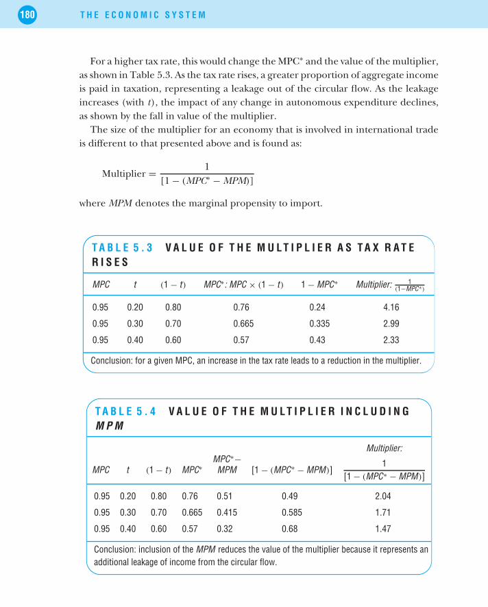
180 T H E E C O N O M I C S Y S T E M
For a higher tax rate, this would change the MPC∗ and the value of the multiplier,as shown in Table 5.3. As the tax rate rises, a greater proportion of aggregate incomeis paid in taxation, representing a leakage out of the circular flow. As the leakageincreases (with t), the impact of any change in autonomous expenditure declines,as shown by the fall in value of the multiplier.
The size of the multiplier for an economy that is involved in international tradeis different to that presented above and is found as:
Multiplier = 1[1 − (MPC∗ − MPM)]
where MPM denotes the marginal propensity to import.
T A B L E 5 . 3 V A L U E O F T H E M U L T I P L I E R A S T A X R A T ER I S E S
MPC t (1 − t) MPC∗: MPC × (1 − t) 1 − MPC∗ Multiplier: 1(1−MPC∗)
0.95 0.20 0.80 0.76 0.24 4.16
0.95 0.30 0.70 0.665 0.335 2.99
0.95 0.40 0.60 0.57 0.43 2.33
Conclusion: for a given MPC, an increase in the tax rate leads to a reduction in the multiplier.
T A B L E 5 . 4 V A L U E O F T H E M U L T I P L I E R I N C L U D I N GM P M
Multiplier:MPC∗−
MPC t (1 − t) MPC∗ MPM [1 − (MPC∗ − MPM)]1
[1 − (MPC∗ − MPM)]
0.95 0.20 0.80 0.76 0.51 0.49 2.04
0.95 0.30 0.70 0.665 0.415 0.585 1.71
0.95 0.40 0.60 0.57 0.32 0.68 1.47
Conclusion: inclusion of the MPM reduces the value of the multiplier because it represents anadditional leakage of income from the circular flow.

E C O N O M I C A C T I V I T Y : T H E M A C R O E C O N O M Y 181
T A B L E 5 . 5 T R A D E S H A R E S O F E C O N O M I CA C T I V I T Y ( % G D P ) 2 0 0 2
USA UK Ireland Germany Japan
X : exports 6.5 18 72 30 10
M: imports −11 −21 −43 −24 −7.5
X − M: net exports −4.5 −3 29 6 2.5
Source: Economist Intelligence Unit, Country Data except for Ireland: Trade Statistics of Ireland, Irish CentralStatistics Office.
Payments for imports represent a further leakage of income from a country’scircular flow, hence the multiplier is different. For a country with an MPM of 0.25,the impact on the multiplier is shown in Table 5.4, which extends Table 5.3.
The extent to which imports and net trade is important for different countriesis shown in Table 5.5 which presents the share of exports (X ) and imports (M) asvalues of each country’s GDP, for a sample of countries.
Both the USA and UK experienced trade deficits in 2002 because the value oftheir imports exceeded their exports. Japan, Germany and Ireland displayed tradesurpluses. Countries’ comparative advantages (see Chapter 2) help us to understanda considerable portion of the international trade that takes place between them.
5 . 7 I N T E R N AT I O N A L I N T E G R AT I O NA key characteristic of the current international economic system is the extent towhich individuals, firms and countries are exposed to influences from foreign goods,services, firms, capital and labour. Individuals and economies are increasingly facedwith contributions by far distant people and places to their lives. Evidence for thisis found, for example, in the growth in international trade.
World growth in exports outstripped world GDP growth between 1995 and2000 by a factor of more than two (7% per annum compared to 3%). Overthe longer period spanning 1948–2002, the figures are 6% for exports and3.7% for GDP (see www.WTO.org for more national and international tradeinformation and statistics).

182 T H E E C O N O M I C S Y S T E M
Trade provides outlets for countries’ output when domestic demand is insufficientto allow firms to sell all produce. The trade option also provides firms in someindustries with the possibility of reaping scale economies, allowing them to reducetheir average costs of production as their output expands. Hence, not only cantrade lead to greater quantities of output produced in an economy in response toaccess to more markets, but it can also generate greater efficiency in terms of howresources are used within economies.
5.7.1 EXPLAINING GROWING INTERNATIONAL TRADEA number of factors explain the growth in world trade. Declines in trade barrierssuch as tariffs and quotas certainly play a role.
Trade barriers are policies or practices that reduce the amount of imports into acountry. Examples include tariffs and quotas.
Import tariffs operate like a tax on goods originating in a different customsarea.
Tariffs raise the price paid by consumers for imported goods making themless attractive to buy. Tariff rates are decided by governments but are increasinglyoutlawed under the WTO. Sufficiently high tariffs on goods for which domesticallyproduced substitutes exist can eliminate any incentive to buy the imports.Governments receive the revenue generated by tariffs.
Quotas raise the price paid by consumers for imported goods making themless attractive to buy. Quotas are quantitative restrictions set by governments onthe amount of imports permitted from another customs area. Because quotaslimit the supply of a good, they drive the price of the goods up.
Declining trade barriers reduces the costs of buying foreign goods for consumersand provides them with greater product choice. Another important explanationlies in the form of falling transportation costs allied to the types of goods currentlybeing traded.
Historically when the majority of goods traded were agricultural products, rawmaterials and processed commodities like steel and meat, their cost of transportationwas high given their weight and bulk. In such a world it made most sense to tradewith countries in close proximity.
A commodity is an undifferentiated product such as wheat or oil or computermemory chips. Commodities are usually of uniform quality, often produced by

E C O N O M I C A C T I V I T Y : T H E M A C R O E C O N O M Y 183
many different producers where each producer’s output is considered equivalentor interchangeable. Futures markets exist for many commodity products.
The majority of traded goods today are finished manufactured products. Due totechnological developments these products often consist of low-weight components(relative to steel) and micro technologies (microprocessors replacing heavy controlpanels) that mean their value relative to their transport cost is high. For manyfirms, low and relatively stable transport costs make shipping such goods beyondthe nearest countries an increasingly viable option.
Shipping technology itself was reorganized from the 1950s with the adventof ‘containerization’, which involved substantially less unloading and reloading ofcargo and hence, lower related labour costs. Ships were redesigned to transport suchcontainers more efficiently. In the 1970s road and rail transportation began to bereorganized and deregulated in the USA – until then the government was involvedin decisions on transport costs and often licensed lorries to ship goods only on oneleg of a return journey. (The Japanese waited until the 1990s before beginningsuch transport deregulation.) Currently, air transportation is being deregulated.Transport deregulation to date has allowed costs to fall, encouraged greater tradeand generated productivity gains for firms in time and resource savings.
Transformation of the transport sector has not just impacted shipping finalgoods to customers but also firms’ coordination of transport and production ofcomponents and intermediate goods produced internationally. Computer andcar manufacturers are prime examples of industries where global coordinationof the manufacturing process has been facilitated by reductions in internationaltransport (and communications) costs. It often makes economic sense to sourcesome components in East Asia, others in the USA and others in Europe and toconduct some sub-component assembly and final assembly in different locations.The complex set of activities that go into sourcing raw materials and componentsand organizing them to create the product sold to customers is all associated with afirm’s supply chain.
A supply chain describes the resources and processes that are involved inacquiring components and raw materials and includes delivery of end products tofinal consumers. It includes the activities of sellers, distributors, manufacturers,wholesalers and any other service providers and contributors to the buyer’sdecision to buy.
To help firms coordinate such activities, supply chain management companies haveemerged. By outsourcing successfully, firms are able to reduce costs substantially.

184 T H E E C O N O M I C S Y S T E M
An outsourcing firm can hold inventories to save on storage costs for its clients,for example. It is also often possible to shorten the time to bring a product tomarket because the logistical maze of procuring components is left to the ‘expert’outsourcing firm which can do so at lower cost by exploiting scale economies.More cost-effective and efficient distribution can also result. The benefits of greaterefficiencies and improvements in time to market can allow businesses that outsourceto reorient their focus towards their most important business activities.
Offshore outsourcing (known as offshoring in the United States) involves relo-cation of elements of the supply chain to a foreign location for more efficientproduction. Both production and services may be outsourced. Because of itslow cost base, China has become an important player in production offshoringwhile India has emerged as a competitive provider of services. (The website ofthe National Association of Software and Service Companies www.NASSCOM.orgprovides information on offshoring activity in India.)
5.7.2 BENEFITS AND COSTS OF INTERNATIONAL TRADEHeated debates ensue about international trade in general and offshoring inparticular. Trade and international integration are viewed, by some, as threats toeconomic stability and growth. On the one hand this is strange since, as we saw inChapter 2, specialization and comparative advantage generate a better internationaloutcome for all countries that trade.
As Adam Smith pointed out in 1776, it is possible for Scotland to producegrapes suitable for wine-making using glasshouse-technology but it would costapproximately 30 times more than available imported wine; it would be difficultto argue in favour of tariffs to encourage Scottish wine production.
Smith highlighted the opportunity cost of limiting trade and encouraging produc-tion in goods for which a country may have no inherent comparative advantage.It may make economic sense for Scottish grape growers to respond to importtariffs by producing wine yet the resource cost (products not produced by thoseresources devoted to wine production) means more efficient and productive useof the resources is not possible. Trade without barriers would leave the Scottisheconomy free to produce and specialize based on its comparative advantage. If thisis true for Scotland and wine then why not for the USA or France or Japan and whynot for components or services as well as products?

E C O N O M I C A C T I V I T Y : T H E M A C R O E C O N O M Y 185
Smith’s Scottish wine example is interesting because the Scots were not producingwine in sufficient quantities for producers to have a strong voice to complain aboutcheaper imports. Nor were sufficient Scottish workers employed in the industry tolobby for the protection of their jobs. These are crucial issues in the context oftoday’s trade debates.
Industry, trade associations and trades unions are often unhappy about theeffects of cheaper imports on their companies’ profitability and members’ jobsand wages, respectively. And so they should be – they are correctly looking outfor their own and their members’ interests. Certainly we can all come up withexamples of jobs which have been moved abroad due to ‘the current internationaltrading environment’ or similar explanations which essentially boil down to loweropportunity costs of production elsewhere. At various points in time, it seems thatsome jobs are inevitably displaced to other locations by imports.
We know that offshoring and imports help domestic companies maintain theircompetitiveness and, hence, support rather than displace domestic jobs. US importsof steel make the Caterpillar tractor company more competitive, allowing it to sellmore, allowing it to provide more jobs. Distributors of tractors could sell morevehicles and farmers get more tractor for their money, allowing them to be morecompetitive. But fewer jobs in the US steel industry result from steel imports.Unemployed steel workers suffer. Others gain.
Price changes and the economic adjustment they bring about always create‘winners’ and ‘losers’ and real income is redistributed as a result.
Deciding to restrict imports protects some industries and domestic jobs but it is notwithout costs.
In the 1980s US restrictions on textile and apparel imports kept prices of suchgoods relatively high. This meant fewer jobs in the clothing retail sector andhigher consumer prices. Estimates of the cost of protecting textile jobs whereannual wages were approximately $15 000 to $20 000 was put at about $50 000per job (Hufbauer and Elliott, 1994).
As a group of disparate consumers and taxpayers funding protectionism, we donot feel the direct link between our tax payments, higher prices and trade policybut it is definitely there. Logically, workers whose jobs are threatened or lost totrade feel the pain and voice their dissatisfaction.

186 T H E E C O N O M I C S Y S T E M
Some jobs are displaced by technological change or product innovations but werarely hear protests in favour of limiting technological improvements or innovation.Arguing for limits on trade seems to be an easy target, implicitly placing more valueon jobs under threat from lower-cost foreign production rather than jobs that maybe created elsewhere in the economy based on its comparative advantages. Froma political perspective this makes sense. Workers who lose their jobs often reflectthis in their voting patterns. Workers who ‘gain’ jobs often do not attribute it tofree trade or the policy of the government of the day. Nor do increased productvariety and lower costs for consumers often appear as underlying people’s votingpreferences.
At the microeconomic level for individuals and for firms, arguing against importscan sometimes seem logical but if it occurred across all areas of an economy, themacroeconomy would suffer and lower aggregate output and per capita incomeswould result.
The fallacy of composition arises here. Although the net effect of trade is positive,this does not necessarily translate into positive effects for every individual intrading countries. The results of trade – availability of a broader variety of goodsand services at lower prices – is easily forgotten by an unemployed worker whosejob has been lost to imports.
From the perspective of developing countries, it is also worth noting that boththe United States and the European Union maintain trade restrictions that harmsuch countries by limiting their ability to export goods. Through the WTO (andits predecessor, the General Agreement on Tariffs and Trade) improvements havebeen attempted but reform has been promised for many years without substantialresults. It is still the case that average tariff levels in agriculture (predominantlyexported by developing countries) are about nine times those in manufacturing.Industrial countries subsidize agriculture, effectively cutting world prices becauseof the supply incentive subsidies create for farmers in industrialized countries.Not only does the EU spend around £2.7bn per year to make sugar profitable forEuropean farmers but it also shuts out low-cost imports of tropical sugar throughtrade barriers.
Minimizing or overlooking the negative microeconomic effects of tradeis a problem with many free-trade advocates. It may well make the free-trade argument more palatable and popular if these issues were dealt withexplicitly.
There is a link between the arguments for free trade and for greater focus onnational income distribution, addressed in Chapter 9. Both require examination of

E C O N O M I C A C T I V I T Y : T H E M A C R O E C O N O M Y 187
the economic repercussions on the least well off of economic measures that maywell favour an economy overall and perhaps even the majority of its citizens. Yet,economic models or explanations indicative of welfare improvements for ‘average’or ‘representative’ citizens should not ignore costs borne by minority groups, whichare insufficiently compensated for their losses.
5 . 8 G O V E R N M E N T A C T I V I T YGovernment exerts its economic influence in a number of ways through its interac-tions with consumers and firms both domestic and foreign. A government’s actionsare important for an economy in terms of its role in setting the tone for howbusiness is conducted generally. While the extent of government activity withinthe economic system varies from country to country, governments’ activities aregenerally focused on a number of goals such as:
• Stabilization policy: Stabilizing the economy by minimizing the short-run fluctua-tions of GDP (output) and unemployment associated with the business cycle.
• Dealing with AS and AD shocks: these are any unpredicted events that causechanges in equilibrium national output and the price level.
• Making transfer payments.
• Public good provision.
• Taxation: to enable government to make transfer payments, to pay for nationaladministration and the provision of public goods. Countries that have largerpublic sectors need relatively high taxes to pay for them.
• Allocating (or reallocating) resources: by making transfer payments and imposingtaxes, the government reallocates/redistributes the economy’s resources.
• Regulation: some markets are regulated by imposing tariffs, quotas, etc. Othermarkets are regulated depending on what competition laws are enacted andenforced (more on this in Chapter 6). Governments also assume responsibilityfor ensuring law and order.
• Creating an environment to support expansion of AS: implementing appropriatepolicies – education, research and development, business support, etc.
Despite a considerable amount of research (e.g. Slemrod, 1995), no clear link canbe established between the size of the public sector and the state of countries’economies. What does seem to be important for economies is the effectiveness ofthe public sector rather than its size.

188 T H E E C O N O M I C S Y S T E M
When a government manages its economy well, its spending plan or budgetcan be met by the revenue generated by the economy. If spending is greater thanrevenues, the government generates a budget deficit while, if revenues are greaterthan expenditure, a government surplus results. Whether the revenue is sufficientto cover the budget depends on the amount of government spending (G), the taxrates (t) levied, and the level of economic activity.
Governments use fiscal policy whenever they affect G or t (which affect aggre-gate demand).
An expansionary fiscal policy is followed if the government manages to increaseactivity by injecting extra income into the circular flow.
A fiscal policy that results in lower activity is described as contractionary andresults in a reduction in the circular flow of income.
If a government tries to stabilize economic activity, this means attempting tomaintain a regular growth rate in real output, with no significant fluctuationsup or down. To implement a stabilization policy, governments should followcontractionary fiscal policy in booms and expansionary policies in recessions tomitigate the affects of the business cycle; such polices would be countercyclical.
Countercyclical fiscal policies have the opposite effect on economic activity to thatcaused by the business cycle, reducing income flows during booms, increasingincome flows in recessions.
To figure out whether governments follow contractionary or expansionary policies,what is at issue is whether the government tries to affect equilibrium output overand above the effects of automatic stabilizers. Examples of automatic stabilizersinclude income tax rates, VAT rates and unemployment benefit.
Automatic stabilizers result in reducing the response of national income tochanges in autonomous spending. They are measures that automatically counterthe business cycle without government action. For example, in a boom, govern-ment net tax receipts rise, taking income from the circular flow.
In the case of a demand shock, such as an unexpected fall in investment demand,aggregate demand falls, leading to a new equilibrium situation in the short run withlower output and a lower price level (sketch this situation using Figure 5.7 as yourstarting point). Depending on the size of the fall in output, this might also lead to arise in unemployment. Firms might keep on all their workers if the drop in output is

E C O N O M I C A C T I V I T Y : T H E M A C R O E C O N O M Y 189
small, but would be more likely to make workers redundant if there was a big dropin output. We know that due to the multiplier effect the total effect on output wouldbe larger than the initial cause of the drop in income/output. However, automaticstabilizers act to stabilize the economy because the drop in income/output wouldautomatically result in a fall in the government’s tax take (due to lower income, thegovernment takes in less revenue in taxes) and, if workers are unemployed, a rise inpayments for unemployment benefit. The drop in tax receipts and rise in paymentsto the unemployed helps people to deal with the decline in income/output. Thesechanges occur automatically in the economy.
Depending on the stage of the business cycle, a government might be receivinghigh or low tax revenues or be paying out high or low amounts in benefits. Tocorrectly assess the discretionary fiscal policy stance of the government requiresremoving the business-cycle impact on government revenues and expenditure.When this is carried out the result is a cyclically adjusted budget, which may show adeficit or surplus.
A cyclically adjusted budget provides information about the discretionary fiscalpolicies a government has followed to deliberately achieve specific macro-economic goals. These might include trying to achieve a particular level ofinflation, or employment or government deficit, for example.
Quite often, as is evident from Table 5.6, governments end up with budget deficits.Borrowing must be repaid and the extent of past borrowing is revealed in countries’national debts. Most countries in Table 5.6 ran deficits in 2003. Sweden alone ran asurplus. Japan is an outlier in terms of its debt situation – it owed the value of over154% of its 2003 GDP in debts.
T A B L E 5 . 6 B U D G E T A N D D E B T S I T U A T I O N , 2 0 0 3 ( A S %O F G D P )
USA UK Ireland Japan France Sweden Germany
Budget balance∗ −3.5 −3.1 −0.2 −7.4 −4.1 0.1 −4.0
Public debt∗∗ 62.4 51.4 32.4 154.6 69.1 52.8 63.9
Notes: ∗Negative data imply budget deficits were run.∗∗This corresponds to the definition used under the Maastricht criteria relevant for European Monetary Union (more on thisin Chapter 7).Source: Country Data, Economist Intelligence Unit.

190 T H E E C O N O M I C S Y S T E M
When public debt increases, economists tend to open the issue to debate. Debtsgenerated for sound economic reasons are not considered problematic but the issueof whether debts are sustainable – i.e. if they can be repaid – is often raised. Debtsneed to be repaid in the future so the cost will be borne by tomorrow’s taxpayers ifthe government borrows today. While voters may desire high levels of governmentspending, high debts may require future high tax rates, and hence will not bepopular with voters. The effects of high tax rates on incentives to work, employmentand running a business may very well create headaches for a government trying torepay future debts and could very well deepen the problem.
Some economists consider that since much of national debt is owed to domesticcitizens, it may not be a problem; the most important consideration regardingdebt is how it is used. Debts generated to invest in infrastructure or educa-tion that will increase future economic activity should help pay for the debt.Debts generated to pay for day-to-day costs like public sector pay or the runningof government departments is more difficult to defend because such expendi-tures should really be met by day-to-day revenues where at all possible, since inmany cases they are unlikely to generate their own revenue streams to be self-financing in the future. Economists should be concerned with the purpose ofexpenditures and the efficiency of expenditure when analysing the sustainability ofpublic debt.
5.8.1 ANOTHER PERSPECTIVE ON ECONOMIC ACTIVITY: THEECONOMY AS A PRODUCTION FUNCTION
Depending on the issue of interest, different models of economic activity areuseful. Earlier the model of aggregate demand and supply was presented. For somepurposes, however, it is useful to view an economy as a production function.
The production function is a relationship describing how economic activity,specifically output, depends on the factors of production and technology. Itdescribes a technically efficient use of the factors of production and technologynecessary to produce output, i.e. no resources are unemployed.
Examples of ‘standard’ production functions are:
Y = F (K, L, T) PF1Y /L = F (K/L, T) PF2Y /L = F (K/L, E) PF3

E C O N O M I C A C T I V I T Y : T H E M A C R O E C O N O M Y 191
For each production function output, Y , is related to the factors of production,which are capital (denoted K), Labour (denoted L) and technology (denoted T).The term F indicates that there is some functional relationship between outputand inputs but because these are general equations, the precise relationship orfunctional form is not specified. The above relationships hold for firms, industriesand economies. If you look back to Figure 4.2, you will see a sample productionfunction for a firm for the short run when capital is fixed. For the focus and purposeof this chapter we refer here to economies.
While the three production functions are quite similar, PF2 and PF3 are expressedin per worker terms. In PF1, output depends on inputs and technology. In PF2 outputper capita depends on capital per worker (K/L) and technology. (Remember thesefactors of production were highlighted earlier as contributing to aggregate supply.)The capital/labour ratio (K/L) of an economy provides information on the capitalintensity of the economy.
Capital intensity is the amount of capital each worker in the economy (onaverage) has at their disposal.
Usually in economies that generate a high level of economic activity, the K/L ratio isrelatively high. In terms of policy options for government, trying to increase this ratioranks quite high. An economy’s capital intensity rises if investment expenditures oncapital machinery and equipment grow faster than what is required just to replacedepreciation of an economy’s capital stock.
In PF3 output per worker depends again on capital per worker and on theefficiency of labour (E). The efficiency of labour itself depends on both technologyand the efficiency of business and general market organization. Explicit inclusionof the efficiency of labour allows for the consideration of learning in the processgenerating economic activity. For example, the efficiency of labour can improveif nothing else in the economy changes except workers’ ability to ‘work smarter’from using their specific knowledge of their job more efficiently. It is often only byon-the-job experience that workers figure out the best ways to achieve their workgoals via learning by doing.
Output (or output per worker) can grow if factors of production increase and areused for production. If the amount of capital in an economy rises due to increasedcapital investment, for example, that economy can grow. This can happen onlyif the capital can be put to productive use to produce something in demand, i.e.for which people are willing to pay. If labour increases output can grow, once (asdiscussed in Chapter 2):

192 T H E E C O N O M I C S Y S T E M
1. there are jobs for the additional labour; and2. those jobs generate sufficient return to cover workers’ wages/salaries, other
business costs and the opportunity cost to the owner of the business.
If technology improves more output (or output per worker) can be producedfrom a given set of inputs which implies improved production methods eitherthrough innovations, invention or better management and organization. Theseimprovements will lead to lower production costs once the technology is nottoo costly.
This production function approach to describing economic activity allows foranalysis of many interesting questions regarding economic activity, although unlikethe aggregate demand/aggregate supply approach, the aggregate price level is notan explicit feature of the approach. Hence, inflation is not directly part of themodel, nor indeed is unemployment. However, the relationship between outputand inputs, technology, the efficiency of labour and the role of learning can beconsidered using the production function approach. Hence, the most appropriatemodel to use when considering economic activity must be chosen based on theissue of interest and the model most suited to that issue. In Chapter 9 we return tothe production function approach in discussing economic growth and its sources.
5 . 9 S U M M A R Y
• Macroeconomic or aggregate economic activity is represented by the circular flowdiagram encompassing all income flows between the various markets in the economicsystem. These include markets for products and services, labour and other factorsof production.
• Standard measures of economic activity are GDP and GNP. Methods for measuringGDP or GNP include the expenditure, income or value-added methods. All methodsshould lead to an equivalent measure.
• The distinction between short and long run is relevant for aggregate economicactivity. In the short run, economic activity displays business cycles. In the longrun, a trend growth rate can be estimated.
• The aggregate demand and aggregate supply model can be used to analyse economicactivity at macroeconomic level and helps us to understand how aggregate nationaloutput (or income) and the average aggregate price level are determined.

E C O N O M I C A C T I V I T Y : T H E M A C R O E C O N O M Y 193
• The concept of the multiplier is crucial to understanding how changes in autonomousspending ultimately impact on economic activity.
• Given the various functions of government, governments affect equilibrium economicactivity through a number of channels.
• For open trading economies, trade creates aggregate benefits, but costs of tradealso arise for some economic units.
• A production function approach is one appropriate model for aggregate economicactivity. This method can be appropriate in analysis of economic activity, dependingon the issue of interest.
R E V I E W P R O B L E M S A N D Q U E S T I O N S1. Separately in the case of firms, households and government, explain all of the
transactions that they are involved in within the circular flow. Make sure todiscuss their role regarding products, services, resources and money.
2. Separately in the case of resource, factor and money markets, explain how youthink local, domestic and international financial systems, systems of corporategovernance, legal and political environments, social and cultural background,technological capability and the myriad standards, business and personalethics, and codes of conduct that are embedded in the economic system allplay a role in understanding the circular flow.
3. a. Using data for five countries of your choice, graph their long-term growthpath from 1950 to the last year of available data (use data from the Gronin-gen Growth and Development Centre website http://www.eco.rug.nl/ggdc/index-dseries.html). Compute the average rate of growth for theperiod overall and for each decade. Try to identify boom periods andrecessions from your graph.
b. For the same five countries as in 3a, compare the growth rate of populationwith real output growth and comment on whether welfare can be arguedto have improved for each country. The data are also available from thesame source.
4. Go to the website of your national statistics provider. Find the section on pricesand plot the trends in average consumer prices for the last five years. Hasthe trend been rising or falling? Compare this trend with the HarmonizedIndex of Consumer Prices for all EU Member States (which is available fromhttp://www.cso.ie/principalstats/princstats.html under the Prices heading).

194 T H E E C O N O M I C S Y S T E M
5. Use an aggregate expenditure curve and an aggregate demand curve (similarto Figure 5.4) to explain what you would expect to happen to equilibriumoutput and the price level if the average price level fell by 5%. Explain theindividual effects you would expect for aggregate demand in terms of the realwealth effect, the interest rate effect and the international trade effect.
6. a. Use the following table to compute the multiplier when the MPC is 0.90and the tax rate is 20%.
Multiplier:
MPC t (1 − t) MPC∗ : MPC × (1 − t) 1 − MPC∗ 1(1 − MPC∗)
0.90 0.20
b. Indicate in the following table what happens to the multiplier if the MPCfalls to 0.85. Explain why this is so.
Multiplier:
MPC t (1 − t) MPC∗ : MPC × (1 − t) 1 − MPC∗ 1(1 − MPC∗)
0.85 0.20
c. Indicate in the following table what happens to the multiplier if the taxrate falls to 15%. Explain why this is so.
Multiplier:
MPC t (1 − t) MPC∗ : MPC × (1 − t) 1 − MPC∗ 1(1 − MPC∗)
0.85 0.15
d. If an MPM of 0.20 is included in the tables above, compute the newmultiplier in each case.
7. For your domestic economy look up appropriate sources to find out andexplain what your government has done in relation to each of the followingover the last three to five years.

E C O N O M I C A C T I V I T Y : T H E M A C R O E C O N O M Y 195
• Stabilization policy, reaction to economic shocks, transfer payments, pro-vision of public goods, taxation, resource reallocation, regulation, policieslikely to encourage expansion of aggregate supply.
8. Use the latest available data from your national statistics provider or the WTO(www.wto.org) to identify the main sectors and goods that your country exportsand imports. Do the same exercise for 10 years previously. What does yourinformation reveal about your country’s comparative advantages?
F U R T H E R R E A D I N G A N D R E S E A R C H
• Two of the greatest minds in economics – Hayek and Keynes – provided theoriesof business cycles. See Hayek, 1975 and Keynes, 1936.
• For research on economic performance and the size of government see Slemrod,1995.
• For analysis of trade related issues, Foreign Affairs contains topical articles.Regarding the offshoring/outsourcing debates see Drezner, 2004.
• Some good books on international integration have been published recently,including Wolf, 2004 and Bhagwati, 2004.
R E F E R E N C E SBhagwati, J. (2004) In Defence of Globalization. Oxford University Press, New York.Drezner, D. (2004) ‘The outsourcing bogeyman’, Foreign Affairs, May/June, 22–34.Hayek, F. (1975) Monetary Theory and the Trade Cycle [original publication 1933].
Augustus M. Kelley, New York.Hufbauer, G. and K. Elliott (1994) Measuring the Costs of Protectionism in the United
States. Washington: Institute for International Economics, 5, 13.Keynes, J. (1936) The General Theory of Employment, Interest and Money. Macmillan,
London.Schumpeter, J. (1975) Capitalism, Socialism and Democracy [original publication
1942]. Harper & Row, New York.Slemrod, J. (1995) ‘What do cross-country studies teach about government involve-
ment, prosperity and economic growth?’, Brookings Papers on Economic Activity, 2,373–431.
Smith, A. (1776) An Inquiry into the Nature and Causes of the Wealth of Nations.Wolf, M. (2004) Why Globalization Works. Yale University Press, New Haven.

C H A P T E R 6
C O M P E T I T I O N I N T H EE C O N O M I C S Y S T E M
By EDWARD SHINNICK
�
�
�
�
L E A R N I N G O U T C O M E SBy the end of this chapter you should be able to:
✪ Explain why competition is a complex process in the economic system.✪ Explain the Austrian perspective on competition as an ongoing process within
an economy which includes an explicit function for entrepreneurs.✪ Describe the traditional models of competition (non-Austrian) using figures
including demand, costs and supply.✪ Compare and contrast the assumptions and outcomes for consumers, producers
and society as a whole, of alternative models of competition.✪ Compare and contrast the traditional and Austrian approaches to competition.✪ Use the five forces framework to highlight the factors that explain why some
industries are more attractive – more profitable – than others.✪ Discuss what is meant by market failure, how it may arise and its implications.✪ Explain what is meant by the structure, conduct, performance paradigm and
how it provided a foundation for competition policy. Explain the implicationsof changes in the formulation of the SCP paradigm for competition policy.
✪ Provide some examples of why competition may give rise to problems foran economy.
✪ Analyse how competition policy can be used to address competition problems.
6 . 1 I N T R O D U C T I O NPrevious chapters have outlined the demand and the supply sides of the economyand how these two elements interact within the economic system. This chapterexplores this interaction further by analysing how and why firms compete in the

198 T H E E C O N O M I C S Y S T E M
marketplace. Pick up any business magazine or newspaper and undoubtedly youwill find a reference to ‘competition’ in a report on the economy. The term iswidely used yet we may not fully understand what it means and its importance. Therole of this chapter is to explore the meaning of competition and the beneficialconsequences of competition for the economy and society as a whole.
The Austrian influence is present again in this chapter with the Austrian per-spective on how competition can be viewed as an ongoing process in the economicsystem outlined in section 6.2. This incorporates the concept of discovery andprovides an explicit role for entrepreneurship as a factor of production.
This is followed in section 6.3 by presentation of the main economic modelsof competition that characterize different industries. These complementary per-spectives on competition in sections 6.2 and 6.3 are compared and contrasted insection 6.4.
In section 6.5 the focus shifts to why markets may not always work to thesatisfaction of governments and what can be done to correct such outcomes. Thisre-introduces the role of government in the economic system and what it can do inthe form of a national competition policy to address market problems. Analysis ofcompetition policy, its aims and how it is implemented completes the chapter.
6 . 2 C O M P E T I T I O N I N T H E E C O N O M I CS Y S T E M
When economists use the term ‘competition’ or advocate greater competition theygenerally have in mind some mechanism that brings about an increase in supplyleading to a reduction in equilibrium price and an increase in equilibrium quantity(ceteris paribus). However, the term ‘competition’ involves much more than just anincrease in supply.
The extent of competition in an economy has implications for a whole set ofinteracting issues such as innovation, efficiency, availability of a variety of goods andservices, and prices that together influence and enhance the welfare of individualconsumers. When individual consumer benefits are aggregated, the economy too isbetter off as a result of competition.
Within the economic system we have a series of interacting agents that actindependently of each other and yet are part of a complex interrelated web. In thecontext of competition, the marketplace is a crucial element in this web where theinteraction of different economic units, each motivated to maximize their utility,results in an outcome that benefits both these individuals and the entire economy.

C O M P E T I T I O N I N T H E E C O N O M I C S Y S T E M 199
Despite the potential benefits from economic interactions, markets do not alwaysoperate to generate positive outcomes. Instead markets can become distorted andcan end up serving one group of people at the expense of others. For example, somemarket conditions result in producers gaining the most from market exchange, whileconsumers end up with fewer benefits (from a consumer surplus/producer surplusanalysis). In such cases, the government may deem it necessary to intervene in themarket to achieve a more balanced outcome, from a public-policy perspective. Suchintervention can take the form of removing restrictions on, for example, quantityrestrictions on supply, on prices or on foreign trade. Arguments for interventionsalso come from lobby groups or vested interests whose focus is on maximizing theirown benefits and depending on the lobby group will adopt either a public-policy orbusiness perspective.
When governments intervene in markets truly open, competitive free marketsdo not exist. There are many examples of how competition is limited by the entryof new firms being blocked or in some way made more difficult. Governmentintervention is by no means the only way in which entry can be restricted butit is one example of restricting competition by setting a limit on the number ofcompetitors in an industry – a case in point is the pub industry where competitionis limited as pubs require licences from the government to operate in that market.Naturally occurring restrictions also occur where a firm has access to the solesupply or knowledge required to produce a good, and examples include oil, andcoke, for different reasons. Barriers to entry can arise due to the type of product(standardized or differentiated), the existence of economies of scale, initial orongoing capital requirements or cost disadvantages independent of size, such asaccess to distribution channels.
Standardized products: products for which many substitutes are available andwhich use readily available technology in their production.Differentiated products: products for which several different varieties are pro-vided (e.g. cars). Differentiation between varieties depends on producers’ choicesof the product attributes for which consumers are willing to pay.
Competition, therefore, is a complex concept that is often not fully understood interms of what it actually means and its implications in the marketplace, for pricesand supply, and therefore for economic growth and employment.
6.2.1 COMPETITION AS A PROCESSOne view of competition is that it is a process whereby through learning over time,economic units on the demand and supply sides of the economy reach a state where

200 T H E E C O N O M I C S Y S T E M
their plans become mutually consistent. Hayek, in particular, and the AustrianSchool of Economics in general, would subscribe to such a view where competitionis a discovery procedure, where people discover knowledge on an ongoing basis.Competition is perceived as being similar to a game of gathering knowledge andexploiting that knowledge for economic gain. The concept of competition as agame has several useful implications. For example, in any game, we do not knowthe results beforehand, skill is required to influence the outcome and the outcomeis unpredictable. The following quote from Hayek (1978) illustrates this point:‘Competition is valuable only because, and so far as, its results are unpredictableand on the whole different from those which anyone has, or could have, deliberatelyaimed at.’ (p. 180)
Unlike in standard games where there are winners and losers (also called zero-sumgames), competition often generates greater gains than losses or costs. For example,the result of a new more efficient competitor entering a market and charging lowerprices might be to put some other firms out of business, but consumers gain fromthe lower prices charged and more efficient use of society’s resources is made.
An important implication of Hayek’s description is that we cannot set out tocreate an outcome that is in itself unpredictable. If competition is a discoveryprocedure, then we cannot know beforehand what is to be discovered. In addition,the outcomes of a game can only be temporary because as new knowledge isdiscovered and used, new outcomes are likely to emerge. Therefore, rather thananalysing whether competition has achieved a particular outcome, we should insteadfocus our attention on making comparisons across similar markets, across industriesand/or across countries and consider which outcomes are economically superior.
This concept of competition is appealing because the knowledge that exists andthat is developed over time within a marketplace is unlikely to be generated asefficiently through any other mechanism. Therefore the miracle of the marketplaceis that it allows the market system to achieve results that are not only unpredictablebut are also the ‘best’ outcome possible.
In a similar vein to Hayek, Schumpeter offered us the notion of competition ascreative destruction (discussed in the treatment of business cycles in Chapter 5).Schumpeter viewed competition as a dynamic process that is based on innovationand change, arguing that in the process of economic growth and in the developmentand expansion of new products, technological change results in the displacement ofold products and old technologies by new products, jobs and technologies. Old jobsand factories become obsolete and defunct and are no longer productive withinthe economic system.

C O M P E T I T I O N I N T H E E C O N O M I C S Y S T E M 201
Knowledge and the use of this knowledge are central to this process-view ofcompetition. As outlined in Chapter 2, such knowledge is dispersed throughoutthe economic system and its application is central to the functioning of this system.Prices become signals of this knowledge. Again Hayek (1978) illustrates this point:
Utilisation of knowledge widely dispersed in a society with extensive division oflabour cannot rest on individuals knowing all the particular uses to which wellknown things in their individual environment might be put. Prices direct theirattention to what is worth finding out about what a market offers for variousthings and services. This means that the, in some respects always unique,combinations of individual knowledge and skills, which the market enablesthem to use, will not merely, or even in the first instance, be such knowledgeof facts as they could list and communicate if some authority asked themto do. The knowledge of which I speak consists rather of a capacity to findout particular circumstances, which become effective only if possessors of thisknowledge are informed by the market which kinds of things or services arewanted, and how urgently they are wanted. (p. 257)
Hayek highlights several useful ideas worth noting. Knowledge plays a central rolein the view of competition as a process, where each individual knows something butnobody knows everything. The existence of tacit knowledge is also recognized, as isthe role of the entrepreneur in discovering and using knowledge in a profitable way.
Tacit knowledge: is highly personal, not easily visible or expressible and cannoteasily be copied. It usually requires joint, shared activities in order to transmit it.Examples of tacit knowledge include subjective insights, intuitions and hunches.
Finally, the concept of demand is referred to in terms of things or services wantedand ‘how urgently they are wanted’.
6.2.2 ENTREPRENEURSHIP, DISCOVERY AND THE MARKETPROCESS
At the heart of the use of knowledge in market economies lies the entrepreneur.
Entrepreneurs exploit knowledge by converting knowledge discovered into prof-itable gain.
Crucial to entrepreneurs’ ability is the freedom to enter existing markets or developnew markets so discovery is fundamental to the notion of an entrepreneur. The

202 T H E E C O N O M I C S Y S T E M
entrepreneur’s skill lies in discovering knowledge and then using the market processto exploit it for profitable gain.
Entrepreneurship is about being alert to a set of opportunities, having a subjectiveexpectation as to the value of such opportunities in the market and having theresources (or ability to generate them) to realize this value.
This may be no more than exploiting a price difference in two markets by buy-ing cheap in one market to sell at a higher price in another market. Such anentrepreneurial discovery will eventually result in the disappearance of the pricedifference (consider the role of the speculator as described in Chapter 7) therebybringing continual change to the market. The notion of equilibrium in the Austrianview of competition can only be temporary since new opportunities continually arisethat cause future change. Entrepreneurship can also involve combining resourcesin a unique way that represents value to the consumer – something for whichconsumers are willing to pay.
Entrepreneurship, by definition, cannot be predicted. It brings chaos to marketsin the sense that it generates price movements and resource allocation and re-allocation decisions and all this is done in the search for economic profit. In theprocess ‘mistakes’ can be made either by incorrectly interpreting knowledge or byincorrectly judging the value consumers would place on such knowledge. Hence,we have some unsuccessful product launches, unsold inventories and bankruptcies.But through the discovery process more knowledge is gained which feeds back intoentrepreneurial decision-making and so the cycle continues.
Competition in the context of entrepreneurship means one thing – free entryinto any market. This is also known as contestable markets.
Contestable markets: markets where entry costs and exit costs from marketsare low.
Without this free-entry condition, discoveries cannot be made and so entrepreneur-ship is restrained. Discoveries could take the form of new technology, resultingin lower production costs (lower average cost curves), or new product attributes,resulting in more value to consumers (reflected in new or higher demand func-tions). Such discoveries would lead to resources being redirected in the economyto where their productivity is highest, and the impact of changes in markets wouldbe reflected in changes in prices.
Discoveries might include a perception on changing consumer tastes. If con-sumers demand more computers and fewer typewriters then, through the market

C O M P E T I T I O N I N T H E E C O N O M I C S Y S T E M 203
mechanism, the price of computers rises while the price of typewriters falls. As theequilibrium quantity changes so too can profits, and increasing profit levels wouldprovide incentives for more producers to engage in the production of computers andfewer producers to engage in the production of typewriters. Changing profit oppor-tunities result in increased computer production. As more computers are producedthe price of computers will eventually start to decrease, whereas falling demand fortypewriters will result in less production and falling prices in that market.
This outcome reflects society’s change in preferences and it unfolded as individ-uals pursued their own self-interest without anyone or any government directingthem to do so. Moreover, the market mechanism also operates as a check on indi-vidual self-interest. Any increases in price by one entrepreneur to take advantageof an additional profit opportunity may well be met with prices actually being biddown by more efficient entrepreneurs entering the market or through a switch tosubstitute goods.
Markets are organized by a self-regulating process and what may seem at the firstinstance to be chaotic and disorderly is, in fact, not.
The marketplace by its very nature is constantly changing with knowledge beingdiscovered, and any equilibrium state is only transitory. A major factor in causingsuch change is innovation.
Adam Smith explained that as markets increase in size, this leads to morespecialization as producers seek better ways to produce goods and more ways toimprove existing products. So both product and process innovation can be as a resultof increased specialization. This is consistent with Schumpeter’s views, introducedabove, that market forces push down profits on existing goods, incentives are createdto introduce new products and processes and avail of greater profit opportunities.
Accordingly innovation is a critical feature in the marketplace and again the entre-preneur is central to this process. This has led to debate on how best to increasethe level of innovation and its by-product – economic prosperity. Patents are one wayto increase innovation activity by providing the entrepreneur with added securitythrough a system guaranteeing protection from imitation, thus encouraging them toundertake costly research and development expenditures searching for knowledgeto be exploited in the market. Consumers gain immediately from patent-protectedinnovations in termsof theavailabilityofpreviouslyunavailableproductsorprocesses.Consumers may also gain over time as the discovery embodied in patents eventuallybecomes dispersed more widely in the economic system once the patent runs out.
A limit to competition in the theory of entrepreneurship is the monopoly controlof unique resources. This control can occur naturally, through ownership rights (that

204 T H E E C O N O M I C S Y S T E M
is, property rights) or through government regulations and the issuing of patents, forexample, both of which have the effect of restricting entry to markets. The presenceof patents in some markets indicates the precedence given to benefits from innova-tion over potential costs from greater market competition. There is a trade-off anddecisions must be made on how the greatest benefit is provided to society.
Other types of barriers to entry that can limit competition are governmentregulations including licensing agreements. This is again related to what rolegovernments should play in the marketplace. Depending on political ideology,some argue for an extensive role for government involvement in the market.Others, such as the Austrian school, believe that government involvement shouldbe kept to an absolute minimum on the basis that any government intervention toprevent a free-market solution attempts to devise alternative allocation mechanismsthat are rarely, if ever, better than the free-market solution. The role of governmentin this latter case would then be limited to supplementing the market process, tofacilitate its smooth functioning.
6 . 3 A LT E R N AT I V E M O D E L SO F C O M P E T I T I O N A N D M A R K E TS T R U C T U R E
Traditional models of competition evolve around four types of market structure,each of which is examined separately below in terms of its implications for a firm’sability to earn profits, which we see is related to a firm’s market power.
Market structure refers to certain characteristics of an industry, such as thelevel of concentration, the extent of entry barriers and the extent of productdifferentiation.Market concentration refers to the number of firms in a specific market and theirrelative market share.Market power exists when firms in a market hold a sufficiently large market sharethat their actions can change the market price of a product – producing moreresults in a falling equilibrium price, producing less leads to a rise in equilibriumprice, ceteris paribus.
At one extreme there can be just one firm in a market and we call this monopoly. Atthe other extreme a market can be characterized by many firms; each small, relativeto the overall size of the market – this is called perfect competition. All examples

C O M P E T I T I O N I N T H E E C O N O M I C S Y S T E M 205
of market structure apart from perfect competition come under the heading ofimperfect competition.
Between the extremes of monopoly and perfect competition there are two ad-ditional forms of market structure: monopolistic competition and oligopoly. Monopolisticcompetition is characterized by many firms each with some power to set the priceof their product, which they hold because they supply a particular brand ofproduct – they differentiate their product. Oligopoly is characterized by a few firmsof large size relative to the total market, so each firm has some degree of marketpower.
Market concentration is often used as the primary measure of market structure.To calculate the level of concentration in a market, a concentration ratio (CR) canbe calculated.
A concentration ratio measures the market share of the biggest firms in themarket. For example a CR4 calculates the market share of the largest four firms.
Even though a concentration ratio only counts the top firms this can be quiteaccurate since if the purpose is to calculate the degree of market power in anindustry, it is assumed the biggest firms have the most power. The Herfindahl Indexis a more accurate measure of concentration.
The Herfindahl Index measures the market share of all firms in the industry bysumming the squares of each individual firm’s market share:
H =N∑
1
S2i
where Si denotes each firm’s market share and summation is from firm 1 to N ,the total number of firms in the market. The squared term indicates that firmswith large market shares will have higher weight.
Market share can be measured in terms of, for example, total sales, net output,numbers employed or capital asset values. However, depending on the measureused, the calculation of market share will differ.
In the airplane manufacturing industry, different measures resulted in differentresults. Boeing and Airbus have both claimed to be the largest in the industry.With just two firms in this industry it should have been obvious that both

206 T H E E C O N O M I C S Y S T E M
could not be correct in their analysis. But as it happens both were right!This happened because each firm used a different measure of market share.Boeing, the older firm and once also the dominant firm in the industry,used the number of airplanes delivered as their measure of market share.Airbus, the younger but rapidly growing firm, used the number of airplanesordered. Using these different measures both firms could claim to be thelargest firm.
Concentration and market structure are the key ingredients in market analysis.
6.3.1 PERFECT COMPETITION
Assumptions underlying this model are:
• Products are homogeneous – all products are alike and so no perceiveddifferences exist.
• All participants in the market have perfect knowledge – full informationon prices, costs and product availability exist.
• There are a large number of buyers and sellers in the market. Each firmprovides a fraction of the output of the industry.
• Firms have no control over price and are, therefore, price takers. Each firm’sdemand curve is perfectly elastic. At the market price, firms can sell asmuch output as they like.
• No barriers to entry or exit exist in the market.
Further characteristics of this market structure include:
• Prices are set by market supply and demand. Market demand is a downwardsloping relationship, while market supply is upward sloping.
• At the market price, firms earn normal profits in the long run, no opportunitiesexist to earn supernormal profits in the long run.
• Factors of production are fully mobile and can be easily transferred from oneindustry or market to another.
• There is efficient use of resources.
How equilibrium emerges in the short run and long run are considered sep-arately below.

C O M P E T I T I O N I N T H E E C O N O M I C S Y S T E M 207
Short-run equilibrium
Figure 6.1 presents the short-run equilibrium for the industry in panel A and thefirm in panel B. Industry price is determined by the intersection of the demandand supply curves in panel A. At the short-run equilibrium price P∗ one firm in theindustry (panel B) can sell as much output as it likes, but will selling nothing eitherabove or below this price. The firm faces a horizontal demand curve at this price.Industry output is Q I, while the firm’s profit-maximizing output Q F is determinedby the intersection of its MR and MC curves.
Since there are many firms in this industry, the quantity each firm produces, Q F,is very small relative to the total output of the industry, Q I. In Figure 6.1, the firmis making supernormal profits since the lower section of its AC curves is below theprice. With each individual firm in a perfectly competitive industry able to earnonly P∗ for its output, P∗ represents a firm’s additional revenue (MR) if it sellsextra output. Since the price the firm receives on any unit of its output is P∗, thisprice also represents the firm’s average revenue (AR) on each unit of output. Withperfectly elastic demand at the price P∗, marginal revenue and average revenue areall given by P∗.
At Q F the firm’s supernormal profit per unit is equal to the distance betweenprice and the AC curve. The firm’s total supernormal profits is represented by thedashed area in Figure 6.1 panel B. If the distance between the price and the ACcurve at Q F is £2 and the firm produces 1200 units (Q F = 1200), then the totalsupernormal profits earned by the firm in the short run is £2400. Conversely, if thefirm’s AC curve is above price then the firm is losing money and it will only survivein the short run if it can cover its average variable costs. As explained in Chapter 4,
A: Industry
P
P*
Output
D
QI
SP
P*
Output
MC
QF
D = AR = MR
AC
AC
D
B: Firm
F I G U R E 6 . 1 S H O R T - R U N E Q U I L I B R I U M I N P E R F E C TC O M P E T I T I O N

208 T H E E C O N O M I C S Y S T E M
the critical short-run survival decision for the firm is whether or not it can cover itsaverage variable costs.
Long-run equilibrium
Logically, the supernormal profits earned in Figure 6.1 will encourage new firmsinto the industry and result in the supernormal profits declining as firms competeby charging lower prices. Firms will not compete by offering different quality goods,as goods are presumed to be homogeneous. Existing or incumbent firms may wishto take advantage of such profitable opportunities and may also increase theiroutput. The net result is a shift of the industry supply curve to the right as in panelA in Figure 6.2.
A new lower industry price results at P1. Panel B outlines the effect of this pricereduction for the same firm considered in Figure 6.1. The firm’s price and AR fallin response to the corresponding fall in the industry price. This reduction in bothindustry price and firm’s AR continues until such time as the AR is tangential to thefirm’s long-run average cost curve (LRAC). Additional industry supply continuesuntil equilibrium emerges where it is just economically profitable for the firm tostay in business, since it can cover long-run average costs. Were the industry priceto fall any further, the firm would be better off exiting the industry in the long run.No further incentive for new firms to enter the industry exists.
No supernormal profits are earned by a firm in a perfectly competitive market inthe long run.
A: Industry B: FirmS0
S1P
P0
Output
D
P1
P0
P1
P
OutputQ
D0 = AR0
D1 = AR1
LRAC
F I G U R E 6 . 2 L O N G - R U N E Q U I L I B R I U M F O R T H EI N D U S T R Y A N D T H E F I R M U N D E R P E R F E C T C O M P E T I T I O N
C O M P E T I T I O N I N T H E E C O N O M I C S Y S T E M 209
Output is produced efficiently in a perfectly competitive industry:
• Production occurs at the minimum point of each firm’s average cost curve.
• The price charged to consumers is the minimum price that could becharged while encouraging firms to stay in the industry.
• Economic resources are used to their maximum efficiency by all firms sinceprices cover marginal costs (this is allocative efficiency).
• Firms earn normal profits but not supernormal profits, so consumer surplusis maximized.
All outcomes indicate the model of perfect competition to be efficient in theory.Of course, very few examples, if any, of perfectly competitive industries exist intoday’s business world. Instead economists tend to use the outcomes of the modelas benchmarks for comparison across all types of market structure.
6.3.2 MONOPOLYIn a monopoly, one firm supplies the entire market. Such cases are quite rare butdo exist. In focusing on the model, we can compare and contrast its implicationswith the perfect competition case.
The assumptions underlying monopoly market structure are:
• There is only one firm in the industry.
• Entry barriers exist to prevent entry by other firms.
• The monopoly firm maximizes its profits.
• The monopoly product has no close substitutes, therefore each monopolyfirm has control over price.
In a monopoly, the firm’s demand function and the industry/market demandfunction are one and the same – a downward sloping demand curve. The monopolyfirm sets its price depending on what it considers the market will bear, evident inthe demand function for its product, given its costs.
The monopolist has a large degree of market power or control over price.
The firm sets price so as to maximize profits, i.e. sets MC = MR at point X inFigure 6.3, leading to the monopoly price Pm and quantity Q m shown. At thisprice the firm earns supernormal profits because the price is above average cost.The dashed area in Figure 6.3 represents the total amount of supernormal profits

210 T H E E C O N O M I C S Y S T E M
Output
D
MR
MC
AC
Qm
X
P
Pm
AC
F I G U R E 6 . 3 E Q U I L I B R I U M U N D E R M O N O P O LY
earned by the monopolist. New firms cannot bid these profits down due to barriersto entry in the industry.
If scale economies imply that only one firm could supply efficiently, i.e. at lowcost to the market, a natural monopoly exists.
Monopolies sometimes have a different shaped AC curve to that shown in Figure 6.3.This can arise from the existence of substantial economies of scale in the industry(see Figure 4.7 to refresh your memory). Scale economies result in average costscontinually falling over large levels of output. This would be the case in, for example,capital-intensive industries such as the rail industry or electricity provision.
Figure 6.4 illustrates the characteristics of the AC curve and equilibrium in suchan industry. Here the monopolist’s AC curve is falling over a large range of output
MR
P
Output
D
MC
LRAC
Pm
Qm
MC = MR
F I G U R E 6 . 4 N A T U R A L M O N O P O LY

C O M P E T I T I O N I N T H E E C O N O M I C S Y S T E M 211
and starts to rise only at very large output levels. Again, the profit-maximizingmonopolist sets MC = MR to maximize profits and earns supernormal profits atprice Pm and output Q m.
This ability to earn supernormal profits under monopoly market structure can bea major cause of concern for governments and competition watchdogs since suchprofits imply lower consumer surplus than if profits were lower.
6.3.3 PERFECT COMPETITION VS. MONOPOLYThe extent of the impact on welfare and consumer surplus is evident from Figure 6.5where perfect competition and monopoly market structures can be comparedand contrasted.
One striking difference between monopoly and perfect competition is theequilibrium price and output levels when facing an identical market demand curve.
Under monopoly price is higher and output is lower than under perfect compe-tition.
This implies that consumer surplus is lower and producer surplus higher undermonopoly, due to this redistribution of income away from consumers and towardsthe monopoly producer. There is also an area that is lost completely in welfareterms, which neither consumers nor producers gain: defined by the triangle abc.This is called a deadweight loss.
A deadweight loss represents the welfare lost to society from relatively ineffi-cient production.
MR
P
Output
D
MCAC
Pm
Qm
Ppc
Qpc
ab
c
F I G U R E 6 . 5 P E R F E C T C O M P E T I T I O N A N DM O N O P O LY C O M P A R E D

212 T H E E C O N O M I C S Y S T E M
Unlike under perfect competition, a monopoly firm does not produce at maximumefficiency since it does not produce at the minimum point of the AC curve (Q pc).Hence, resources are not used at maximum efficiency since under monopoly outputis restricted.
Given these seemingly negative consequences of monopolies, why do they exist atall? Because the underlying assumptions of product homogeneity and free entry andexit in the perfect competition model rarely if ever hold true in the business world!
The challenge for the economic system is to acknowledge that perfect compe-tition is not achievable and to ensure that the beneficial effects of competitionare maximized.
Barriers to entry exist in many industries and these impede the ability of new firmsto come into the market and bid down price.
Barriers to entry may be based on:
• Type of product: standardized versus differentiated products. The ability offirms to differentiate their products and thereby create brand loyalty canmake it difficult for new entrants to gain a foothold in a market, especiallyif consumers are unwilling to switch from a brand they know and trust.
• Economies of scale: Some industries require the firm to produce a relativelylarge output in order to operate at or near the minimum point of theiraverage cost curve. In this case the ability of the firm to secure a largeoutput will determine whether they can profitably enter the market. In theextreme case of the average cost curve continuing to fall over large outputranges, only very large firms could compete or, in the natural monopolycase above, just one firm would be profitable.
• Experience curve effects: Sometimes experience by the incumbent firm in theindustry can result in lower average costs for that firm. New entrants whotherefore do not have this experience are faced with higher average costs.This puts them at a competitive disadvantage.
• Capital requirements: Some industries require a large amount of initial capitalin order to set up production. A firm’s ability to access such capital maydetermine their ability to enter the market.
• Cost disadvantages independent of size: Incumbent firms may have long-established relationships with suppliers or distributors that give the firmvaluable access to important resources. Dealing with a long-established

C O M P E T I T I O N I N T H E E C O N O M I C S Y S T E M 213
supplier over a period of time can provide the firm with access to a reliablesource of high-quality raw materials at competitive prices at a time that suitsthe firm’s production schedule. A new entrant, not having such access, maybe at a competitive disadvantage.
• Legal protection: The firm’s ability to secure patents can prevent a newentrant from competing in the market. Licences granted by, for example,national governments, or trade agreements between countries would havesimilar effects.
Benefits from monopoly?
Despite the potentially negative aspects of monopolies, there are instances wheremonopolies generate economic benefits. Central to the positive aspects of monopo-lies is their potential for innovation, emphasized by Schumpeter. The supernormalprofits that monopolies earn can be used for investment into R&D facilities. How-ever, this is only a positive result for society if firms carry out such investment ratherthan squandering their profits. There are some incentives that may encouragemonopoly firms to invest, at least, a proportion of their profits back into the firmand these incentives centre around the ability to earn higher profits in the future as aresult of successful innovation and thereby securing their dominance in the market.
Other arguments in favour of monopolies centre on their ability to exploiteconomies of scale in production such that society reduces wasteful inefficiencies.If a monopolist can gain efficiencies over and above those that could be gained in aperfectly competitive market (if small output shares are produced only at relativelyhigh average cost) then monopolies have advantages. Coupled with such advantagesis the potential, which always exists in monopolies, to exploit a market position andin doing so harm consumer interests. Critics of monopolies point to this potentialdamage as outweighing any potential advantages and will therefore be sceptical ofthem, especially as there are many cases where innovation and R&D take place innon-monopolistic industries.
6.3.4 MONOPOLISTIC COMPETITIONMarkets characterized by monopolistic competition, first described by EdwardChamberlin, involve many sellers producing products that are close, but not perfectsubstitutes – there is product differentiation. Each firm has a monopoly in its ownvariety of the product. Examples of monopolistic competition include restaurants,petrol stations, corner shops and builders. This market structure is illustrated inFigure 6.6.

214 T H E E C O N O M I C S Y S T E M
P
Output
D
MR
MC
LRAC
P*
Q*
F I G U R E 6 . 6 L O N G - R U N E Q U I L I B R I U M U N D E RM O N O P O L I S T I C C O M P E T I T I O N
The assumptions of market structure characterized by monopolistic compe-tition are:
• Large number of sellers each with a relatively small market share. Firms donot have to be overly concerned with what rivals are doing and how theyare likely to react.
• Firms produce differentiated products – gives them some power over pricebut close substitutes are available – demand is elastic.
• Freedom of entry to the industry exists. Supernormal profits in the shortrun attract new entrants and new varieties so that long-run supernormalprofits are not made.
• There is full and symmetric information – a new entrant takes market sharefrom all competitors equally.
In the short run, any supernormal profits earned by a firm will disappear as newentrants enter the market, offering substitute products and attracting some cus-tomers, resulting in the demand curve facing each other firm declining – shifting tothe left. In the long run, the demand curve is tangential to the long-run AC curve andnormal profits are earned at price P∗ and quantity Q ∗. The industry is competitivecontaining several competing firms where none makes supernormal profits. Eachfirm produces along the negatively sloped portion of their LRAC, implying scaleeconomies are not fully exploited, implying there is excess capacity in their plant.
With respect to efficiency, each firm does not produce at the lowest point onthe LRAC curve; therefore, production is not efficient. Also since price exceedsmarginal cost, each firm has some degree of monopoly power, created through theexistence of brand loyalty.

C O M P E T I T I O N I N T H E E C O N O M I C S Y S T E M 215
M A I N TA I N I N G A N D E N H A N C I N G B R A N D L O YA LT Y I NM O N O P O L I S T I C C O M P E T I T I O N
Incumbent firms purchase advertising and other promotional activities, whilenew entrants may have to spend substantially more in order to gain a footholdin the market. Advertising is one example of non-price competition and it is amajor feature of this type of market structure. By spending on advertising, firmsnot only want to gain new customers but also keep existing customers; that is theywant to make their customer’s demand curves more inelastic. Yet advertising isexpensive so firms must balance the perceived benefits of advertising against theactual costs of advertising.
How do firms do this? They continue to spend on advertising so long as theadditional (marginal) revenue the advertising brings in exceeds the additional(marginal) cost of the advertising. Firms’ profits increase as long as MRadvertising >
MCadvertising. Advertising exhibits diminishing marginal returns, such that moreand more advertising will yield less and less revenue so eventually MRadvertising =MCadvertising and the firm’s advertising adds nothing to profits.
6.3.5 OLIGOPOLY
The final type of market structure considered is oligopoly.
The underlying assumptions of oligopoly are:
• Few sellers exist in the market – each taking account of the decisions oftheir competitors.
• Products of each firm are similar but not identical.
• Each firm produces a substantial amount of output and so has mar-ket power.
• Barriers to entry exist.
Oligopolies occur where a market has ‘room’ for a few large firms. This couldbe because of cost advantages through scale economies or through economies ofscope.
Economies of scope exist when a firm produces many products and can shareresources across them such that the unit costs of each product is lower than ifthey were produced by separate firms. Shared marketing or distribution costsmay be sources of economies of scope.

216 T H E E C O N O M I C S Y S T E M
In industries where mergers and acquisitions are commonplace (such as thecar industry discussed in Chapter 4) the number of competitors decline asfirms’ business strategies guide them to ‘grow’ not by expanding the mar-ket, which is becoming saturated, but by buying up rivals, which may reducecompetitive behaviour and allow for increasing profit margins once barriers toentry exist.
The essence of oligopoly markets is that firms’ decisions are interdependent.When making decisions on output, for example, each firm takes account of howtheir rivals are likely to respond, as this will affect the profitability of such decisions.This complicates firms’ decision-making processes because it can be very difficultto predict how each rival will respond and precisely how such responses will impacton the firm. Very often firms will seek out a ‘simpler’ solution. For example, insteadof trying to guess how a rival will respond, firms may wish to seek agreements withtheir rivals on output (or other decisions) so as to maximize the profitability withthe minimum of risk. With few firms in an industry this is not as difficult as it mayfirst seem. Yet at the same time there are incentives for each firm to ‘go it alone’so that it can get one step ahead of its rivals. This inherent conflict in oligopolymarkets make for fascinating study.
Formal collusion by firms can take the form of a cartel where firms make explicitoutput agreements, for example, with the intention of maintaining a high price forthe product.
A cartel is an agreement between firms to cooperate in restricting the amount ofoutput they produce, thereby influencing the price.
OPEC (the Organization of Petroleum Exporting Countries) is possibly the mostwell-known cartel and its agreements on levels of oil production (or extraction) foreach country effectively controls the price of oil on world markets (this example isdiscussed in terms of its effects on international inflation in Chapter 8). However,there are two problems with cartels that inhibit their usefulness. First, cartels tendto be unstable because of each member’s incentive to cheat on the agreement andmake extra profits in the short term. When other firms see the agreement breachedthey would follow suit and, in the case of OPEC, increase oil production, therebycausing the world price to fall. Second, in a lot of countries, including Europeand the USA, cartels are illegal and any such agreements are prohibited undercompetition law.
As a result firms may engage in less obvious forms of collusion.
Implicit collusion may take the form of price leadership, where either

C O M P E T I T I O N I N T H E E C O N O M I C S Y S T E M 217
• a dominant firm in the industry sets price and all others follow and set theirprice with this information at hand; or
• a well-established firm becomes the ‘leader’ in the industry and is trustedwith setting the price that all firms will charge.
Such a leader has usually gained the respect of the other firms and has a lotof experience in the industry. All types of implicit collusion are also illegal andtherefore firms may not readily engage in such activities, despite the potentialbusiness benefits.
Oligopoly and game theory
Without collusion in oligopoly markets, firms make assumptions on how rivals react.Such interdependence can be analysed using game theory.
Game theory is a microeconomic approach or tool of analysis applied to under-stand the behaviour of individuals and firms. Pay-offs generated by followingdifferent strategies can be compared.
In game theory, a firm makes assumptions on how the other firm(s) will react andthen chooses its best option. In such games the firm seeks a dominant strategy.
A dominant strategy is one that provides one firm with the best outcome,irrespective of the strategy another firm (or firms) chooses.
Firm interdependence and dominant strategies can be illustrated using the exampleshown in Table 6.1. Here we have two firms; A has two strategic options, X or Y , and
T A B L E 6 . 1 G A M E T H E O R Y :S T R A T E G I C O P T I O N S A N DD O M I N A N T S T R A T E G Y
Firm B’s strategic options
I (high) II (low)
Firm A’sstrategicoptions
X (high)Y (low)
(3, 4)(4, 3)
(2, 5)(4, 5)

218 T H E E C O N O M I C S Y S T E M
firm B has two strategic options, I and II . For firm A, Strategy X could be to set ahigh price and strategy Y to set a low price while for Firm B, Strategy I is high priceand II is low price. By examining the pay-offs from each strategy we can analyse if adominant strategy exists.
Here, if firm A chooses strategy X (high price) and firm B chooses strategy I(high price), then A earns £3 in profits and B earns £4. If A chooses strategy Y(low price) while firm B still chooses strategy I (high price), then A earns £4 and Bearns £3 since lower prices entice consumers to buy more from firm A. When firmB chooses I (high), strategy Y (low) earns firm A higher profit.
When firm B chooses strategy II (low), firm A earns £2 with strategy X (high) and£4 with strategy Y (low). Again strategy Y earns Firm A higher profits. Thereforestrategy Y is a dominant strategy for firm A; no matter what strategy firm B chooses,firm A will always do best by choosing strategy Y .
Similarly for firm B, no matter what strategy firm A chooses, firm B always doesbest by choosing strategy II , so II is B’s dominant strategy.
The equilibrium outcome in this game has firm A choosing strategy Y and firmB choosing strategy II . This outcome earns £4 for firm A and £5 for firm B.
Dominant strategies for either one or both firms result in a relatively easydetermination of the outcome. However, dominant strategies do not exist forall cases.
Consider the Game in Table 6.2. Firms A and B again have two strategic optionsbut with different pay-offs. In this game no firm has a dominant strategy. The firmsare faced with two possible options:
• Option 1: Firm A chooses X and firm B chooses I – each firm earns £10 profit.
• Option 2: Firm A chooses Y and firm B chooses II – each firm earns £5 profit.
T A B L E 6 . 2 G A M E T H E O R Y :S T R A T E G I C O P T I O N S W I T H N OD O M I N A N T S T R A T E G Y
Firm B’s strategic options
I II
Firm A’sstrategicoptions
XY
(10, 10)(0, 0)
(0, 0)(5, 5)

C O M P E T I T I O N I N T H E E C O N O M I C S Y S T E M 219
This is an example of a game with two Nash equilibria (after John Nash, the NobelPrize winner in economics, 1994), where each firm is doing the best it can, giventhe strategy being pursued by the other firm.
A Nash equilibrium exists when each player in a game chooses their best strategygiven the strategies followed by other players.
The two remaining options are less likely since both firms earning zero profits.Therefore, it is crucial that each firm chooses either option 1 or 2 and option 1 ispreferable to option 2 for the firms concerned. But how can the firms ensure thateither of these options will prevail? Collusion would ensure they do not end up withthe worst outcome of £0 profits each.
In the absence of collusion there is still a way for the firms to achieve the betteroutcome. If one firm invests in a commitment of resources that will make it clear toall other firms that it intends to pursue one particular strategy, then this can guidethe second firm in its strategy decision. For example, if firm A invests in a system ofproduction that makes it clear it must pursue strategy X , then firm B, will do bestby choosing strategy I and the resulting profit outcome for both firms is £10. Suchan investment must be both visible and irreversible in order to convince firm B thatstrategy Y will be the strategy pursued by firm A. Pay-offs as before.
To make this example more tangible, consider that strategy X (and I ) involveabiding by an agreement to restrict output and strategy Y (or II ) represent cheatingon such an agreement. If both firms abide by the agreement, they both earn £10; ifthey both cheat, they earn £5. Any deviations from these two strategies will result inzero profits for both, due to, for example, resulting price wars. To achieve the bestpossible outcome one firm could invest in machinery, or a production line, whichis capacity-constrained – only a certain capacity can be produced. Such a firm couldcredibly commit a certain level of production. An agreement could then be madeto set this level of production to maximize their profits.
Prisoner’s Dilemma
An interesting outcome unfolds if the pay-offs to this game were as shown inTable 6.3. Such a game is an example of the Prisoner’s Dilemma.
A Prisoner’s Dilemma exists when the equilibrium from a game generates asub-optimal outcome for all parties involved. With commitment (or a bindingcontract) between the firms, higher pay-offs could be achieved to the benefit ofboth players.

220 T H E E C O N O M I C S Y S T E M
T A B L E 6 . 3 G A M E T H E O R Y :S T R A T E G I C O P T I O N S W I T HS U B - O P T I M A L S T R A T E G Y
Firm B’s strategic options
I II
Firm A’sstrategicoptions
XY
(10, 10)(15, 3)
(3, 15)(5, 5)
High price (or low output) strategies are X and I in Table 6.3, while low price (highoutput) strategies are Y and II . If both firms have low price strategies (Y and II ),industry output is high and profits are relatively low at £5 per firm. With both firmsfollowing high price strategies resulting in low industry output, profits rise to £10per firm. Firms’ profits are maximized at £15 if one firm follows a low price (high
T A B L E 6 . 4 S U M M A R Y O F M A R K E T S T R U C T U R EC H A R A C T E R I S T I C S
No. of Power of Barriers Non-priceType of product firms Examples firm: price to entry competition
Perfectcompetition
Homogeneous Many None None None None
Monopolisticcompetition
Differentiated Many Retailing,buildingandrestauranttrades
Some Low Advertisingand productdifferentia-tion
Oligopoly Standardizedordifferentiated
Few Steel, carand com-puterindustries
Some High Advertisingand productdifferentia-tion
Monopoly Unique One Microsoft A lot Veryhigh
Advertising

C O M P E T I T I O N I N T H E E C O N O M I C S Y S T E M 221
output) strategy when the other firm adopts the alternative strategy (earning £3);combined profits of £18 would be generated.
If firm A thinks B will select strategy I (high price), A’s best option is to chooseY (low price) since its profits of £15 > £10. If B selects II , A’s best option remainsY since £5 > £3. Similarly, B’s best option is to select strategy II . Hence, when noco-operation is possible between firms a non-cooperative equilibrium emerges withpay-offs of £5 to each firm. This is sub-optimal when both could earn £10.
Some co-operation such as a binding commitment or a contract between thefirms could generate an incentive for them both to simultaneously choose X and I(where profits of £20 shared equally are possible). This would be an example of aco-operative equilibrium.
Summary of market characteristics
To sum up this section, the main differentiating characteristics of each marketstructure are presented in Table 6.4.
6 . 4 A U S T R I A N A N D T R A D I T I O N A LP E R S P E C T I V E S : A C O M P A R I S O N
The previous two sections present very different perspectives on competition, i.e.the Austrian ‘competition as a process’ view and the perspective of competition as atimeless state of events. Competition is a dynamic process in the former and a staticprocess in the latter.
Knowledge and its use are key issues distinguishing the traditional view ofcompetition from the Austrian view. In perfect competition, knowledge is ‘perfect’or available to all. Decision-making becomes a problem not so much of makingchoices, but one of maximizing a series of price possibilities from a given set ofresources. Individuals are in a sense ‘programmed’ to select a transaction that is a‘maximum’ outcome attainable. Since knowledge is given, in effect, there is nothingto compete over. All producers and consumers know what is to be known aboutproducts and prices and there is no need to compete for anything.
In reality, characteristics of goods and what makes them scare and valuableare not known in advance and these are some of the issues that the events wecall competition attempt to discover. In perfect competition, the decision-makerdoes not exercise genuine choice; everything is known in advance so there are nochoices to be made. Consequently, it is assumed that no errors are made in thisdecision-making/maximization process.

222 T H E E C O N O M I C S Y S T E M
To many consumers and producers the ‘perfect competition’ dramatization ofthe marketplace is not realistic. In making decisions, individuals rank objectives andavailable resources and in this process new knowledge is gained. This new knowledgebecomes, in turn, part of future ranking processes. In addition, outcomes are notknown in advance; instead individuals are confronted with choices to be made.
The Austrian perspective acknowledges the experience and learning of individu-als where knowledge is not only limited, it is also constantly developing over time.Knowledge is crucial and central to the process of competition itself. It not onlyemerges from competition but also creates competitive forces. Every player in themarket possesses different degrees of knowledge and can use it in exchanges tomaximize their utility, the more specific in nature is the knowledge (as discussedin Chapter 2). This approach is intuitive from our own experiences as consumers.When we purchase goods we do not, and cannot, know everything there is to knowabout the good we are buying, the number of sellers of that good and the pricescharged in different markets. Yet we do not need to know all this information inorder to trade. We simply assess the amount of value or utility that we can derive fromthe product and decide whether the price subjectively represents good value to us.
Another feature of the perfect competition model is that no one firm can gainmarket power. Firms do not interact, they are price takers and accept given ‘world’prices. Yet in business we see many firms with market power and they achieve thisthrough, for example, superior use of knowledge or resources.
Microsoft has become a very large and successful firm by developing a usefuloperating system for personal computers. In the process it displaced IBM, theprevious leader in the industry. The amount of knowledge and, in particular,the use of knowledge that each firm had discovered allowed this situationto emerge.
Equilibrium, central to the traditional model of competition is considered in theAustrian approach as contradictory to the whole notion of competition. Equilibrium,by its very nature, assumes a steady state where the market has absorbed all relevantinformation and is in a position of stability from where there is no tendency tomove – there is no more competition. As we can see from our discussion of theAustrian perspective, though, this can never be the case as knowledge constantlychanges. Therefore equilibrium not only does not exist, moreover it cannot exist.
A further point that sets the Austrian perspective apart from the traditionalmodel is that markets are unpredictable. Competition is more like a game of chancerather than a set of predictable moves and counter moves. This unpredictability

C O M P E T I T I O N I N T H E E C O N O M I C S Y S T E M 223
comes from the central economic problem facing society, that is, the problem ofthe utilization of knowledge which no one individual possesses. Furthermore, thiseconomic problem always arises due to changes occurring in the economy. Hayek(1978) sums up his position as follows:
the point to keep constantly in mind is that all economic adjustment ismade necessary by unforeseen changes; and the whole reason for employingthe price mechanism is to tell individuals that what they are doing, or cando, has for some reason for which they are not responsible become less ormore demanded. (p. 261)
Such change brings with it certain opposition. Competition is generally seen tobenefit the consumer and indeed some producers, but it also introduces new waysof doing things that are better than current methods, the ‘old’ being replacedby the ‘new’. With such displacement comes changing fortunes of those involved.Competition brings with it increased rewards for some and diminished reward forothers. As explained in relation to trade in Chapter 5, such diminished rewardsform the basis on which competition is usually opposed.
6 . 5 W H E N M A R K E T S F A I LThe portrayal and outcomes of competition describe how the self-motivated actionsof consumers and producers leads to production and consumption of goods andservices in an efficient, effective manner, given the incentives generated by theprices of goods and services. However, there are some events that occur that caninterfere or even prevent this outcome – markets can sometimes fail.
Market failure occurs when economic resources are not allocated efficientlycaused by the price system working imperfectly.
6.5.1 WHY MARKETS MAY FAILThe principal types of market failures are public goods, externalities, naturalmonopolies and monopoly power and information asymmetries. These are impor-tant in the context of policy as they provide the rationale underlying much of thegovernment intervention in markets that we observe.
Public goods
Public goods (introduced in Chapter 1) are generally available to all, such that itis difficult if not impossible to exclude any person, even if they have not paid for

224 T H E E C O N O M I C S Y S T E M
the good, from consuming it. Markets often fail to encourage private firms fromsupplying such goods.
Externalities
As outlined in Chapter 4, an externality may result from a production or consump-tion process that affects some individual(s) not directly involved in the process.
Positive externalities are private timber forests providing scenic benefits toall or immunization against contagious diseases in a community. Negativeexternalities are pollution from a factory harming local farmers or cigarettesmoke reducing the enjoyment of a meal by another person.
Often, the prices of products do not fully reflect the true costs including theexternal effects of their production. It is the negative externalities that economistsare mostly concerned with as they reduce the economic welfare of producersand/or consumers.
Natural monopoly and monopoly power
Monopoly power, or substantial power over price, is closely associated with thenatural monopoly case such that a lower level of output may be produced and ahigher price charged than in a more competitive market. These negative aspectscan be sustained due to barriers to entry in the market, which facilitates theredistribution of income away from consumers and towards producers, thus harmingconsumer interests. Monopoly power also provides firms with the opportunity ofengaging in anti-competitive practices, either on their own against other producersor potential producers or against consumers, which effectively means raising pricesabove competitive levels.
Information asymmetries
Information asymmetries exist when one party has more information thananother party in an exchange agreement.
Information asymmetries usually arise where a producer has more information on aproduct or service than consumers who are open to potential exploitation, usually inthe form of high prices and/or poor quality. The functioning of competitive marketsdepends on the ability of consumers to adequately judge competing products. A

C O M P E T I T I O N I N T H E E C O N O M I C S Y S T E M 225
lack of information naturally impedes this. If firms have market power they may havefew incentives to produce relevant information for consumers or the informationmay be of such a technical nature that few consumers would be properly able tointerpret and use it. The information asymmetry problem is most pronounced forexperience goods as against search goods.
Experience goods are goods where their quality attributes can only be assessedthrough trial (or experience) whereas the quality of search goods can be gainedbefore purchase.
The resulting problems are of inefficiency and welfare loss.
6.5.2 IMPLICATIONS OF MARKET FAILUREOne implication of market failure is the redistribution effects from producersto consumers. Society may also suffer a deadweight loss, as considered earlier inFigure 6.5. This is particularly damaging since potential benefits are lost to theeconomy. By preventing such a loss someone in the market place would gain. InFigure 6.7 panel A we have a market performing efficiently where price and quantityemerge from the interaction of demand and supply as PE and Q E. If the quantity ofoutput is limited below its free-market level (for example, because producers canset high prices as fewer goods than the equilibrium quantity may be sold due todistribution agreements) to Q L, consumers pay higher prices at PH. At a higherprice, consumer surplus falls and producer surplus rises but we see that some ofthe original surplus is no longer part of consumer or producer surplus – this is adeadweight loss shown as a triangle in Figure 6.7 panel B.
P
Output
PE
QE
S
P
Output
D
PE
S
QL QE
Producersurplus
Consumersurplus
PH
Consumersurplus
Producersurplus
Deadweightloss
D
A B
F I G U R E 6 . 7 D E A D W E I G H T L O S S

226 T H E E C O N O M I C S Y S T E M
Preventing or correcting market failures can create positive economic benefitsand can provide a justification for government involvement in the market. In anextreme case market failures can prevent a market from existing at all – hence theprovision of public goods.
A government can control the behaviour of producers and consumers through‘indirect command’ where they provide incentives by making certain activities moreor less rewarding. Government involvement can take the form of intervention in themarket, either as a direct supplier of a good or service, or as a policy instrument toforce a positive outcome arising from a market failure. For example, governmentswill usually provide public goods such as national defence and security and alsomay provide the goods associated with natural monopoly characteristics, such as inthe utilities industry where governments have in the past supplied electricity, gas,telecommunications, water, etc.
Less direct government involvement arises in attempts to reduce the impact ofother types of market failure.
• To reduce information asymmetries governments can introduce regulationscompelling producers to release accurate and affordable information in theform of standardized product labelling, setting minimum safety and healthstandards or banning false or misleading advertising.
• Governments can also step into the market, in the form of regulation, to reducewelfare losses arising from negative externalities.
• To reduce monopoly power and reduce the effects of anti-competitive practices,the government can introduce a specific legal instrument in the form of com-petition law, to enforce standards and a policy of competition in the economy.
6 . 6 G O V E R N M E N T R E G U L AT I O NO F C O M P E T I T I O N
Across Europe, governments’ role in reducing monopoly power and in anti-competitive practices has evolved substantially over recent decades, particularlyfrom the 1980s on. One traditional response – for governments to step in andtake ownership of natural monopolies and to impose strict regulations on businessactivities – was considered to be an efficient method until the realization emergedthat it may also generate significant costs. This conclusion arose from:
C O M P E T I T I O N I N T H E E C O N O M I C S Y S T E M 227
• weighing up of the costs versus the benefits of regulations;
• comparing whether the restrictions imposed under regulation were proportion-ate to the potential harm done in their absence;
• examining whether there was a more efficient way of achieving the goalsof regulation.
Furthermore, it was possible in some circumstances that governments’ regulationsmight harm consumers. This occurs if business interests are put ahead of consumerinterests and if there is a weak consumer voice. Both of these can result inregulatory capture.
Regulatory capture occurs where regulations set up to protect consumers – tolead to greater competition and lower prices – become captured by the industryfor the benefit of producers in that industry. This happens where producers canconvince the government or a regulator to introduce rules favouring producers.
Furthermore, the notion of a natural monopoly and the role of governments inrunning such enterprises began to change. Advances in technology and the devel-opment of financial markets, for example, both helped to change the perceptionof natural monopolies. No longer were such industries considered to be optimal ifoperated by one firm and instead many were broken up into small sub-industries. Forexample, in the electricity market, four sub-industries were developed comprising:
• generation: the production of electricity by either hydro, nuclear or fossil fuels,for example;
• transmission: the transfer of electricity from the generation site through thenational grid to different parts of the country;
• distribution: the transfer of electricity from the national grid to local grids andsub-stations;
• supply: the transfer of electricity to homes and industries.
The idea then was to introduce competition into as many of these sub-industriesas possible. Generation and supply were sub-industries where competition wasseen to be possible whereas transmission and distribution were considered to havenatural monopoly-type characteristics. Hence, it did not make economic sense tohave duplicate transmission and distribution networks when the product could betransferred more efficiently through just one.

228 T H E E C O N O M I C S Y S T E M
When introducing different competitors in rail transport, it would not makeeconomic sense to have separate tracks and stations for each train operator.If this were to happen, hundreds of train stations would be scattered aroundthe country, along with thousands of miles of train track. Exactly the samescenario applies to gas, water and other utility industries.
In addition, governments also reconsidered their ownership of certain industries,driven in some cases by EU policy. Moves towards privatization were not only anattempt to bring the benefits of competition to industries, including improvingefficiency, but also to reduce bureaucracy and political interference.
Privatization: the sale of government-owned businesses (and associated assets)in whole or in part to the private sector. Examples include electricity, gas andtelecommunications industries.
Governments’ entire industry philosophy changed, becoming broadly less inter-ventionist in industry with a redirection of their efforts to other policy issues. Theidea was to introduce competition where competition was possible and to haveregulation where it was not. Such regulation could take the form of access/priceregulation so that competitive supply industries could gain access to a product at a‘fair’ price and then sell it on to the end user for a ‘reasonable’ profit where therelevant regulator would decide on the interpretation of fair and reasonable.
Many regulations no longer serving their purpose – either because they wereoutdated, or had been captured by industry – encouraged a process of deregulationor re-regulation of private industry – where old rules were abandoned or amendedto reflect current market conditions. At the same time the EU pushed for greaterliberalization of markets as part of its drive for a single European market. The resultwas a changing competitive landscape in many industries including airlines, utilitiesand some professional services.
Market liberalization: reducing barriers to the free movement of goods andservices to encourage entry by new competitors.
With liberalized markets came government competition policy to ensure a fair andlevel playing field for all competitors. Broad-based competition policy is seen as lessburdensome than industry regulations in attempting to create a well-functioningmarketplace.

C O M P E T I T I O N I N T H E E C O N O M I C S Y S T E M 229
Competition policy at the national level mirrors EU competition policy estab-lished under the Treaty of Rome. Two sections of the treaty form the foundationsof national competition policy in individual EU countries.
Section 81 of the Treaty of Rome prohibits any collaborative agreement betweenfirms whose aim is to prevent, distort or restrict competition within the EU.
Section 82 prohibits firms with market power from distorting competitionwithin the EU.
Competition law is the legal instrument used to enforce competition policy. Thefinal stage in this process was the establishment of competition agencies to monitorand police government competition policy at the national level.
6.6.1 COMPETITION SPECTRUM
If we consider competition as a spectrum with perfect competition at one end andmonopoly at the other, then the role of government in the competition arena is totry to maximize the positive effects associated with perfect competition and avoidor minimize the negative aspects associated with monopoly. Even though these twopositions are extremes, and thus rarely exist in practice, they are still very usefulconcepts if we consider them as representing two opposite ends of the competitionspectrum.
As theoretical abstractions, models of market structure are useful in so far as weknow that the greater the level of competition, the greater are the incentives to:
• drive price down towards costs;
• provide incentives to reduce costs; and
• develop new products that consumers are willing to buy.
So the closer an economy moves towards the perfect competition end of thespectrum, the greater the possibility of achieving efficient allocation of resources,efficient production and dynamic efficiency.
6.6.2 STRUCTURE, CONDUCT AND PERFORMANCE
Much of the basis for thinking on competition originates from the structure,conduct, performance (SCP) paradigm. When this first emerged in the 1950s(e.g. Bain, 1956), a one-way causal relationship was considered to exist between the

230 T H E E C O N O M I C S Y S T E M
structure of a market, the conduct of firms within that market and the performanceof the firms.
Structure: e.g. the number of firms and the market share of each, the extent ofentry barriers and the extent of product differentiation.Conduct: e.g. the ability to practise price discrimination (charging differentmarket segments different prices for the same product – as with airline seats inthe same class) the pursuit of efficiency improvements, the setting of prices (highor low) and the pursuit of strategies aimed at preserving monopoly power ordiscouraging competition.Performance: e.g. profitability, efficiency levels or the quality of the product.
Empirical studies of different industries indicate that the proposed one-way causalrelationship was in fact multidirectional, with all three issues affecting each other.So, for example, the competitive conduct of firms pursuing efficiency improvementscan result in other firms finding themselves unable to compete and thus leavingthe industry, thereby affecting the structure of this industry. The result was areformulation of the paradigm as
S ⇔ C ⇔ P
This paradigm provided insights for thinking about how to change the performanceof firms. Governments realized that if they wanted market performance to changethen market conduct and/or market structure had to change first. Explicit ruleswere introduced as part of achieving such change. The result was governmentcompetition policy.
6.6.3 COMPETITION POLICYCompetition policy has both economic and social objectives. The economic objectiveis based on the view that markets are an efficient mechanism for the allocationof scarce resources. Building on the ideas of Hayek, the knowledge containedwithin the market therefore exceeds the knowledge that even the ‘best’ regulatorsor government legislators could possess. The aim of a policy of competition is tobreak down barriers to new entry or dismantle business practices that discouragecompetition among existing firms. Once this can be achieved, the market makesdecisions of resource allocation. The anticipated result is one of increased resourceefficiency, increased innovation and a reduction in prices at the microeconomiclevel. These microeconomic effects then can lead to macroeconomic effects such as

C O M P E T I T I O N I N T H E E C O N O M I C S Y S T E M 231
increased employment and productivity, through the efficient production of moregoods and services, leading to increased prosperity for society.
The social objective of competition policy can be achieved only if the aboveeconomic objectives are first achieved, since the social objective is based on theaggregate (positive) outcome of the economic effects in the wider economy. Theseinclude the diffusion of economic power and the maximization of opportunitiesfor all.
There is an inherent conflict within competition policy. It may allow firmsto become:
• large enough to gain efficiency through economies of scale;
• profitable enough to enable firms to invest in R&D and develop newproducts/processes.
But large scale may:
• generate market power;
• lead to harmful anti-competitive practices for other (smaller) firms andconsumers.
A delicate balance needs to be struck between these two potential conflicts, andcompetition policy attempts to achieve such a balance.
Principles of competition policy
The USA and the EU are at the forefront in advancing competition policy. Over theyears both US and EU competition policy have converged and common standardsof evaluation have been developed.
In the USA competition policy (or Antitrust as it is referred to) began withthe Sherman Act of 1890, which was enacted largely in response to growingconsolidation of big companies. The Act made illegal any restraints on competition.Interestingly, the one exception to this was any monopoly that was based on applyinga superior technology or offering new products. This was an attempt to encourageinnovation by providing firms with the opportunity to gain substantial profits fromsuccessful innovations. The Clayton Act of 1914 further strengthened competitionpolicy by restricting specific practices if they could substantially lessen competitionor if such practices could lead to a monopoly. This Act was introduced to restraininstances of economic power that were beginning to emerge.
The goal of EU competition policy is to establish a system which safeguardsagainst the distortion of competition, either by restraints placed by private firms or

232 T H E E C O N O M I C S Y S T E M
by government involvement. It explicitly acknowledges the potential for nationalgovernments to distort competition and this has significant effects on the provisionof state aid (as in the airline industry, for example). EU competition policy wasestablished under the EU Treaty of 1957 and the two pillars of this policy are Articles81 and 82, cited above, which prohibit contractual restraints on competition andprohibit an abuse of a dominant position. Rules governing mergers came into effectin 1990.
Table 6.5 summarizes the benefits of competition broken down into the benefitsto consumers, businesses and the economy as a whole.
Implementation of competition policy
If the objectives of competition policy are to be met then proper and full implemen-tation of the policy is essential. This involves an analysis of some key issues, such asthe identification of competitors, the identification of a firm’s product market andidentification of the firm’s geographical market, which may be more complicatedthan they first appear.
Identification of competitors is typically based on the degree of substitutionbetween two products, where substitution is measured by the cross-price elasticityof demand.
T A B L E 6 . 5 S U M M A R Y O F B E N E F I T S O FC O M P E T I T I O N
Consumers:
Price, quality, choice, innovation and bargaining power
Example: airline industry prices reduced by: 25% (UK), 33% (USA), 50%(Spain), 65% (Ireland) accompanied by large increases in demand
Business:
Freedom to enter new markets and win market share
Benefits as buyers of production inputs – as for consumers above
Economy:
One-off effect of increased competition
Lower prices and higher output over time
Increased productivity, innovation and competitiveness

C O M P E T I T I O N I N T H E E C O N O M I C S Y S T E M 233
It is important to make a distinction here between direct and indirect competitors.
Indirect competition arises when the strategic choice of one firm affects theperformance of the other due to strategic reaction by a third firm.
For example, innovation in the tyre market can bring about new competitivepressures in the car market if one car manufacturer uses the tyre innovation toattract customers. This recognizes the dynamics taking place in the market whereaction by one firm provokes a reaction by a series of other firms.
With direct competitors, two products tend to be close substitutes when they havesimilar uses and are sold in same geographic area.
In the world aviation market, Boeing’s 737–800 jet and the Airbus A321 jetwere considered by both Ryanair and easyJet to be close substitutes when theyentered negotiations with both producers to add to their fleets. Both aircrafthave similar passenger and range capabilities. In a local housing market twohouses of similar size, in the same neighbourhood, may be considered closesubstitutes.
Identification of a firm’s market is important, but difficult.
Two firms are in the same product market if they constrain each other’s abilityto raise price.
There are two markets that need to be considered: the product market and thegeographical market. A market is well defined if customers could not switch betweenavailable substitutes in response to a hypothetical small but permanent relative priceincrease by all firms in the market. In other words, would a firm’s customers switchto available substitutes or to a different supplier located elsewhere in response to aproposed permanent price increase of say 5%? If substitution were possible and thismade the proposed price increase unprofitable, due to the resulting loss in sales,then these substitutes would form part of the same ‘market’.
For a geographical market definition the flow of goods and services acrossgeographic regions must be analysed. The idea here is to first find out wherecustomers come from and then find out where the customers shop. A crucial issuein this analysis is transportation costs. Where such costs exist this would imply thatidentical products in two different geographic markets might not be substitutes.

234 T H E E C O N O M I C S Y S T E M
As we saw in Chapter 5, advances in technology can reduce the importance oftransportation cost, and the same is true with Internet shopping, for example.Once the market is defined, the most appropriate measure of market sharemust be identified and the relevant data accessed in order to compute accuratemarket shares.
Examples to illustrate the main issues in competition policy are provided below.The first example deals with mergers and the problem of defining the marketin order to measure market share and therefore potential power/dominance.For those interested in case materials, a good starting point for EU material ishttp://europa.eu.int/comm/competition/index en.html and for US material ishttp://www.ftc.gov/ftc/antitrust.htm.
C O M P E T I T I O N P O L I C Y E X A M P L E 1 : A C Q U I S I T I O N
In 1986 Coca-Cola wanted to acquire Dr Pepper and the US authoritiesinvestigated whether such an acquisition should be allowed. In that yearCoca-Cola was the largest seller of carbonated soft drinks in the USA, whileDr Pepper was the fourth largest. Coca-Cola wished to expand Dr Pepper’smarket by applying its own skills in marketing and at the same time keepingup with its main rival – Pepsi-Cola – also expanding at the time. How to definethe market became the central issue in the case to determine whether theacquisition could proceed. Coca-Cola’s market could potentially be definedas the market for carbonated soft drinks, the market for cola drinks or themarket for all drinks (including tap water). Depending on the definition used,the proposed merger would have left Coca-Cola with either significant or nosignificant market share, and this would naturally have very different effectson competition. Coca-Cola considered the relevant market definition to bethe wider ‘all drinks’ market. However, in this case the market was definedas carbonated soft drinks and data was produced to show that the proposedmerger could increase Coca-Cola’s market share by over 4.5% at the nationallevel and by as much as 10% to 20% in many geographical markets. On thisbasis the proposed merger was blocked.
C O M P E T I T I O N P O L I C Y E X A M P L E 2 : S U B S I D I E S
At the EU level, the issue of state aid where national governments providedsubsidies to companies of national interest arose in several cases. One of

C O M P E T I T I O N I N T H E E C O N O M I C S Y S T E M 235
the most common industries affected was airlines. In the early 1990s theEuropean Commission announced that airlines would no longer qualify forstate aid and put forward a proposal that aid could be given to assist withrestructuring on a ‘one last time’ basis under which Iberia Airlines receivedalmost $1bn in 1992. In 1994 the Spanish government provided Iberia with afurther $1bn in aid to avert bankruptcy. The credibility of the ‘one last time’policy was further diminished when, also in 1994, the Belgian governmentgave financial aid to Sabena. The EU then adopted the ‘market economyinvestor principle’ in deciding whether state aid is anti-competitive. This prin-ciple stated that if state aid takes place in circumstances that would not beacceptable to a private investor under normal market economy conditions,then such aid would be banned. In 2001 Belgian airline Sabena requestedstate aid to fight off bankruptcy arising from industry shocks. It was refusedand the airline subsequently went out of business. The Irish airline, AerLingus, also requested state aid in 2001 and was also refused. It faced thestark choice of restructuring or going out of business. Following restruc-turing the company subsequently turned significant losses into substantialprofits, indicating that state aid is not the only option for a company facingbankruptcy.
C O M P E T I T I O N P O L I C Y E X A M P L E 3 : M A R K E T A B U S E
This case involved British Airways (BA) and Virgin Airlines and concernedthe issue of market abuse. Here BA had 40% of the market for ticket salesin the UK and the next largest competitor had sales of 6%. BA was sub-sequently deemed to have dominance when other factors such as numberof routes and its control over a large number of landing slots were fac-tored in. Virgin took issue with BA over its commission scheme to travelagents. The scheme paid agents 7% for ticket sales on top of a ‘performancereward’, which paid up to an additional 3% on international flights and1% on domestic flights, by matching current year sales to levels of perfor-mance in the previous year. This incentive scheme was seen as persuadingagents to sell more BA tickets, thus giving BA an unfair advantage againstother airlines. BA claimed that these rewards were linked to cost savings andefficiencies and had no damaging effects on other airlines. The EuropeanCommission did not accept these arguments and ruled that such a scheme wasabusive.
236 T H E E C O N O M I C S Y S T E M
6 . 7 S U M M A R Y
• Efficient functioning of a market economy depends on a robust state of competition.
• Through competition knowledge is discovered and exploited in the marketplacethrough the use of the price system.
• If markets are not contestable, entry barriers result in different market structures,ranging from monopolistic competition to oligopoly to monopoly, each with differenteffects on consumers, in terms of their ability to maximize their welfare and onproducers in terms of their ability to earn supernormal profits.
• Market failure is used to justify government intervention in markets in the formof direct controls (becoming increasingly uncommon), or it can take the form ofregulations or rules governing the behaviour of firms. Since all such rules imposecosts on businesses it is important to assess the perceived benefits of these rulesagainst their costs.
• Competition policy is an instrument to impose strict rules of competitive behaviouron firms. One aim is to reduce the role of government involvement in the economyand yet curb any negative effects from market failures. Competition law is the legalenforcement for competition policy and creates incentives for firms to obey sucha policy.
R E V I E W P R O B L E M S A N D Q U E S T I O N S
1. How does Schumpeter’s view of competition as ‘creative destruction’ link with
the idea of competition as a process?
2. Patents prevent firms from copying inventions or innovations by other firms.
Discuss what you think might happen if patents were eliminated so that firms
could imitate successful innovations by other firms.
3. What are the key features of the following market structures: perfect compe-
tition, monopolistic competition, oligopoly and monopoly? If perfect competi-
tion does not exist in practice, what is the purpose of the model?
4. Use a diagram to show equilibrium price and quantity for a monopoly firm.
Explain why supernormal profits result under monopoly. What are possible
negative effects resulting from monopoly? Why do monopolies persist, given
their possible negative effects?

C O M P E T I T I O N I N T H E E C O N O M I C S Y S T E M 237
5. With reference to the pay-off matrix below explain what you understand bythe terms
• dominant strategy;
• Nash equilibrium;
• co-operative equilibrium.
Firm B’s Strategic Options
I II
Firm A’sStrategic Options
XY
(10, 10)(5, 15)
(15, 5)(18, 18)
6. In comparing the Austrian and traditional approaches to competition, whatare the main conclusions? Would you see the Austrian and traditional views asbeing substitutes for or complementary to each other?
7. What is meant by ‘market failure’ and what might cause markets to fail? What,if anything can be done in response to market failure?
8. What is the structure, conduct, performance paradigm? What is the relationshipbetween this paradigm and competition policy?
F U R T H E R R E A D I N G A N D R E S E A R C H
• For analysis of the US, UK and German manufacturing sector considering theefficiency of large scale production see Chandler, 1990.
• For the SCP approach to industry analysis see Bain, 1956, esp. pp. 1–19.
• For a modern applied perspective on markets, market structure and efficiency(among other issues) see Kay, 2003, particularly Parts 3 and 4.
• For consideration of a range of ‘mythical’ examples of market failure seeSpulber, D. (ed.), 2002.
R E F E R E N C E SBain, J. (1956) Barriers to New Competition. Harvard University Press, Cambridge,
Mass.Chandler, A. (1990) Scale and Scope: The dynamics of industrial capitalism. Harvard
University Press, Cambridge, Mass.

238 T H E E C O N O M I C S Y S T E M
Hayek, F. (1978) New Studies in Philosophy, Politics, and History Ideas. University ofChicago Press, Chicago.
Kay, J. (2003) The Truth about Markets: Their genius, their limits, their follies. Allen Lane.Spulber, D. (ed.) (2002) Famous Fables of Economics: Myths of market failures. Blackwell,
Mass.

C H A P T E R 7
M O N E Y A N D F I N A N C I A LM A R K E T S I N T H EE C O N O M I C S Y S T E M
�
�
�
�
L E A R N I N G O U T C O M E SBy the end of the chapter you should be able to:
✪ Explain the three functions of money and describe how money under-pins exchange.
✪ Define what is meant by money and clarify alternative definitions (broador narrow).
✪ Describe how banking systems work to create money.✪ Outline the main motives underlying demand for money.✪ Use the demand and supply model to describe how demand for and supply
of money interact to determine the equilibrium interest rate and quantityof money.
✪ Describe the relationship between real and nominal interest rates.✪ Explain the relationship between money supply and inflation.✪ Apply the demand and supply model to the foreign exchange market to study:
• how demand for and supply of currency interact to determine equilibriumexchange rates and quantity of currency exchanged;
• the causes and consequences of changes in equilibrium exchange rates.✪ Illustrate how the activity of speculators has potential to generate both costs
and benefits in the economic system.✪ Describe how monetary policy works and outline difficulties experienced in
implementing such policies.✪ Explain the logic underlying adoption or non-adoption of single currencies.
7 . 1 I N T R O D U C T I O NSo far we have implicitly used the concept of money in our discussion of theeconomic system. We mentioned the circular flow of income and output which we

240 T H E E C O N O M I C S Y S T E M
measure in money terms. Quite often the role of money is taken for granted butgiven its central role in the operations of an economy, it requires specific analysis.In fact the role played by money in the economic system is complex. Focusingon money and its place in the economy we realize even more the organized andinterdependent nature of the various features and units within the economic system.For instance, what we consider as money today has no value other than that whichwe are happy, by convention, to afford it.
To be used as money, coins, notes, plastic cards (or whatever) must meet anumber of criteria, set out in section 7.2. The supply of money in an economyis organized via central banks and commercial banks as explained in section 7.3.To allow us to analyse the money market we next consider demand for moneyin section 7.4 focusing on motives that explain demand. Bringing supply anddemand together in section 7.5, we can consider how equilibrium is determined.The difference between real and nominal data is addressed once again, althoughhere it is with reference to the ‘price’ of money – the interest rate.
The potential relationship between money supply and inflation is addressedin section 7.6, which also focuses on how monetary policy might be used to tryto control inflation and affect interest rates. The focus then moves to broaderinternational money markets with consideration of how exchange rates are deter-mined, again using a demand and supply approach. This has relevance forcentral banks since one of their functions is to maintain the stability of theirnational currency.
The activities of speculators in foreign exchange markets has received muchattention in recent times and this activity is examined in section 7.8 with interestingoutcomes regarding the potential benefits speculators may bring to markets.
Section 7.9 focuses on monetary policy and how it can be used to affect economicactivity. The final section assesses the arguments underlying monetary integrationfocusing on the specific case of the euro.
7 . 2 M O N E Y A N D E X C H A N G ELife would be considerably more complicated were it not for money to the extentthat we almost take it for granted and certainly do not consider the various functionsit serves.
The various functions of money are:
• medium of exchange;

M O N E Y A N D F I N A N C I A L M A R K E T S I N T H E E C O N O M I C S Y S T E M 241
• unit of account;
• store of value.
Starting with the medium of exchange function, we know when we hand over theagreed amount of money in any transaction, we receive something we want andvalue in return. Whether we hand over cash, cheque or plastic (credit card) weknow that there is agreement that our ‘money’ will be accepted in transactions.The fact that money is light and easily portable certainly facilitates exchange andjust thinking about how barter systems work (where goods rather than money areexchanged for other goods) reveals how much more straightforward it is living in amonetary rather than a barter economy.
That we treat money as a unit of account means that it is the general languagewe use to quote prices and compare them. It would be possible to use any goodas a unit of account if we were all happy to measure prices in mobile phones, forthe sake of argument. This would mean that the price of tables, chairs, books andgroceries would all be quoted in terms of the number of mobile phones requiredto buy them. In theory its sounds possible, but in practice who would want to carryaround mobile phones to pay for everything they buy? And what about the differentphones that are available – this would require an exchange rate relationship to bedeveloped where the purchasing power of one phone would be quoted relative toanother. Even if all prices were quoted in a more basic unit of account, like gold, thisstill would not get around the problem of having to carry around the gold to pay forpurchases. History also reveals that when gold coins were used as an acceptable unitof account, some dishonest people engaged in shaving off some of the gold fromthe coins, thus devaluing them, but without the knowledge of the person acceptingthe gold. Since we are generally unwilling to treat commodities such as gold orphones as a unit of account, we require an alternative. This alternative is fiat money.
Fiat money exists where paper with no intrinsic value itself fulfils the functionsof money, and government legislation ensures that it must be accepted fortransactions.
By convention and tradition we are willing to accept paper and certain coins aspayment because we have monetary systems that we trust sufficiently.
Since not all of consumers’ purchases are made out of current income – peoplesave and borrow – money must also be durable enough to allow for purchases tobe made in the future or loans to be paid back. Money fulfils this function since itcan be kept from one period to another although its purchasing power may not beexactly the same. In that way it can be said to be a store of value.

242 T H E E C O N O M I C S Y S T E M
7 . 3 L I Q U I D I T Y, C E N T R A L B A N K SA N D M O N E Y S U P P LY
Different examples of financial assets exist that fulfil the functions required todefine them as ‘money’; for example, notes, coins, bank deposits, credit cards,travellers’ cheques. Other financial assets such as stocks, shares, or governmentbonds could not be described as money since they cannot be exchanged for goodsand services until they are first converted into money. The easier it is to use afinancial asset to buy goods or services, the more liquid it is said to be.
In general a country’s currency and ‘money’ are managed by its central bank,which deals with the formulation and implementation of monetary policy and tries topromote a sound and efficient financial system in which its citizens have confidencein the sense that they trust that their currency fulfils all the functions money should.Later in this chapter examples of monetary policies and their effects are considered.
Monetary policy is the broad term used to describe how the supply of moneyis regulated in an economy, including how inflation is controlled and how thestability of the currency is maintained.
The amount of money held by banks in their reserves plus the currency in circulationis known as the monetary base.
Different central banks have their own definition of what constitutes money inthe sense of which more and less liquid assets are included. For example accordingto the Federal Reserve, the central bank in the United States (the Fed), thereare three definitions of what is included as money, from very narrow M1 includingessentially the notes and cash and bank deposits available immediately for purchases(including travellers’ cheques) to broader definitions called M2 and M3 that includeless liquid financial assets. (The definitions used by the European Central Bank(ECB) are similar but not exactly the same.) The monetary base is smaller than M1or M2 and only changes with specific activities of the central bank (explained laterin this section). Recent figures for the different definitions of money are providedin Table 7.1 for the USA and Europe.
We can draw the supply curve for money (defined as M1, for example) as shownfor the USA for April 2003, shown in Figure 7.1. The money supply is drawn asa vertical line because the decision about the quantity of money to supply to aneconomy is independent of the rate of interest. When discussing the price of money,

M O N E Y A N D F I N A N C I A L M A R K E T S I N T H E E C O N O M I C S Y S T E M 243
T A B L E 7 . 1 M O N E Y I N C I R C U L A T I O N , U S A A N DE U R O P E , A P R I L 2 0 0 3
US ($bn) EU (¤bn)
Currency M1 M2 M3 Currency M1 M2 M3
642 1236 5921 8600 337 2423 5027 5949
Sources: http://www.federalreserve.gov and http://www.ecb.int
PMS
Quantity ($bn)1236
F I G U R E 7 . 1 M O N E Y S U P P LY : U S A , A P R I L 2 0 0 3
again like any other price we refer to its opportunity cost. The price of money isthe rate of interest since the cost of holding onto money in its most liquid formsis the interest that could be earned if it were on deposit or used to buy a financialasset.
The main channel open to the central bank for affecting money supply is throughopen-market operations.
When the central bank buys or sells government bonds it conducts an open-marketoperation.
Government bonds are issued to generate funds for the government and usuallymature after ten years or more. Buyers of bonds pay money in return for an agreedrate of return on their investment in the future. If the central bank wants toincrease money supply it buys government bonds from the public thereby releasingadditional money into supply. To reduce the money supply the central bank couldsell some of its own reserves of government bonds thus taking money out ofcirculation and transferring it into its reserves.

244 T H E E C O N O M I C S Y S T E M
A further mechanism central to the determination of the money supply in aneconomy is the required reserve ratio held by banks.
The required reserve ratio is the percentage of all deposits received by banks thatmust be held in the bank and not used for loans or other purposes.
Through the required reserve ratio, banks manage to create money, therebyincreasing the supply of money, in an economy. Central banks indicate what thedesired reserve ratio is and commercial banks must retain that specified amountof reserves. Reserves are held so that any depositors requiring to withdraw theirdeposits are sure to be able to do so and will have confidence in their bankingsystem. If on average, the central bank observes that banks need to hold 8% of theirdeposits for customers wishing to withdraw their deposits, this will be the preferredreserve ratio. For a ratio of 8%, a bank that has deposits of £50m must retain £4min reserves but it is free to loan out the remaining £46m as it sees fit, within theguidelines set out by its central bank.
Since banks must hold a fraction of their deposits in the form of reserves, thebanking system is known as a fractional reserve system.
The incentive for banks to loan out funds is generated once the interest they pay ondeposits is less than the interest they can charge on loans so they can make profits.Since the banking market contains several competitors, each bank needs to ensurethat its interest rates compare well to those offered by other competitors.
7.3.1 THE MONEY MULTIPLIER
If loans are created, they produce money in the economy in a multiplicative mannerbased on the money multiplier. This is easily explained using an example. Takingthe case of the hypothetical BankOne, which has reserves of £4m and deposits of£50m. We can consider what happens to the money supply if the bank receives anadditional deposit of £1000 from a customer, Moneybags Inc.
BankOne’s deposits rise to £50 001 000 so it needs to increase its reserves at thecentral bank by £80 (8% of £1000). When the reserves have increased by £80,the remaining £920 can be loaned out by the bank. If a loan of £920 is issuedto Grandon’s, Ltd, their account at the bank is credited with this amount, thusincreasing deposits by £920 to £50 001 920. As deposits rise, reserves must increase

M O N E Y A N D F I N A N C I A L M A R K E T S I N T H E E C O N O M I C S Y S T E M 245
T A B L E 7 . 2 M O N E Y C R E A T I O N V I A T H EM O N E Y M U L T I P L I E R
Assuming a required reserve ratio of 8%
Deposit £ Required reserves £ Loan £
Moneybags 1000 80 920
Grandon’s 920 73.6 846.4
Next customer 846.4 67.7 778.7
Next customer 778.7 62.3 716.4
. . . . . . . . . . . .
Total 12 500 1000 11 500
in line and 8% of £920 is £73.60. When £73.60 is held in the bank’s reserves, againthe remainder of £846.40 (£920 – £73.60) can be used for loans by the bank. Thenthe bank can issue a further loan to Safelock Ltd, which is credited to their accountin the bank, increasing bank deposits, requiring an addition to the bank’s reserves. . . and so on as shown in Table 7.2.
This process ensures that the initial addition to the bank’s deposits generates anincrease in the money supply considerably greater than the initial change.
The money multiplier describes how a change in money supply leads to anultimate change in money supply by a multiple of the initial change.
The size of the money multiplier depends on the required reserve ratioaccording to the formula:
Money multiplier = 1required reserve ratio
Since the ratio is 8% in the example, the money multiplier is 1/0.08 = 12.5. Thismeans that any change in deposits will lead to an increase in the money supply12.5 times the initial increase. If the initial change is £1000 it generates £12 500in additional money supply as shown by the process in Table 7.2. Hence, bankscreate money.

246 T H E E C O N O M I C S Y S T E M
7 . 4 M O N E Y D E M A N DTaken together, money supply and money demand determine the equilibrium priceand quantity of money in the money market.
We hold money or demand money (in more liquid forms) for different pur-poses – for transactions, as a precautionary measure and for speculative purposes.These are known as the motives for holding money.
The transactions demand for money relates to the medium of exchange function ofmoney in that it is the demand for day-to-day spending on things like groceries, busfares, and so on. The amount of money people demand for their transactions willvary depending on their income – generally those earning more spend more – andon the general price level – if prices are high, then relatively more money is neededto pay for purchases.
The precautions demand for money relates to the money demanded for unex-pected emergencies and is again associated with the money’s medium of exchangefunction. The amount of money demanded for precautionary purposes againdepends on individuals’ incomes, and their age.
The transactions and precautionary demands for money are known as the demandfor active balances because the money is actively used to buy goods and services.
The price of money – the interest rate – is not of interest in explaining the demandfor active balances.
The third motive for money demand is for speculative purposes. This motiveis related to money’s store of value function because individuals concerned aboutthe value of financial investments in the future who are afraid the value of theirinvestments will fall prefer to hold money rather than financial assets.
The speculative demand for money is also called the demand for idle balancessince it relates to the desire to demand money to avoid potential losses fromholding interest-bearing financial assets.
The demand for speculative purposes depends on the interest rate, which is theopportunity cost of holding money. With a relatively high rate, people will preferthe more attractive option of holding interest-bearing assets rather than more liquidforms of money.
Figure 7.2 shows the demands for active, idle and total money balances. Note thatthe price of money P is the interest rate. This demand for money or the liquidity

M O N E Y A N D F I N A N C I A L M A R K E T S I N T H E E C O N O M I C S Y S T E M 247
Demand for activebalances
P
Q
Demand foridle balances
P
Q
Demand for totalbalances
P
Q
A B C
F I G U R E 7 . 2 M O N E Y D E M A N D : L I Q U I D I T YP R E F E R E N C E C U R V E
preference curve is shown in Figure 7.2 panel C , which is the sum of the demandfor active and idle balances. This indicates the desire for holding assets in liquidform, i.e. cash rather than in other financial asset forms.
7 . 5 T H E M O N E Y M A R K E T: D E M A N DA N D S U P P LY
Equilibrium in the money market requires an assessment of both demand andsupply together, as presented in Figure 7.3. The opportunity cost of money isdetermined by the intersection of demand and supply, and this is shown as r∗ inFigure 7.3 panel A.
If there is a fixed quantity of money supply then, depending on the demandfor total balances, the interest rate may vary as shown in the comparison betweenFigure 7.3 panels A and B. In both panels the money supply is the same and moneydemand is different. The intersection between demand and supply gives rise to aninterest rate r∗ in panel A, while it is higher at r∧ in panel B. The demand formoney in panel B is greater than in A (the demand curve in panel B is above andto the right of that in panel A) but because supply is fixed the price must rise tobring the market to equilibrium. If the interest rate did not rise the demand fortotal balances at r∗ would exceed the available supply – there would be a shortageof money – and the market would not clear.
In Figure 7.3 panels C and D we can examine what happens when the centralbank conducts open-market operations and expands the money supply (when itbuys government bonds). Initially the interest rate is r∗ but once the open marketoperation increases the supply of money the interest rate declines to r+.

248 T H E E C O N O M I C S Y S T E M
Demand for totalbalances
Interestrate
Q
Money supply
r*
Demand for totalbalances
Interestrate
Q
Money supply
r^
r*
Demand for totalbalances
Interestrate
Q
Money supply
r*
Demand fortotalbalances
Interestrate
Q
Moneysupply
r+
r*
A B
C D
F I G U R E 7 . 3 M O N E Y M A R K E T : D E M A N D A N D S U P P LY
The interest rate must decline when the supply expands because, as shown inFigure 7.3 panel D, at the original interest rate of r∗ the expanded money supply isgreater than demand at that price. The market only clears if the interest rate dropsto bring demand and supply together.
7.5.1 WHICH INTEREST RATE?Figure 7.3 simplifies the process by which the interest rate is determined becausethere is more than one interest rate determined in an economy at any time. Forexample, one interest rate is charged for mortgages. Mortgages are a feature ofthe capital rather than the money market since they are long-term debts – debtsshorter than one year are features of the money market. Another interest rate isearned on deposits held by savers, while another is earned on deposits held for onemonth, or three months, and so on. Two main elements help to explain differencesin interest rates:
• Loan term: loan repayment periods vary in time; some are short like theovernight borrowing that some banks engage in with their central bank, others

M O N E Y A N D F I N A N C I A L M A R K E T S I N T H E E C O N O M I C S Y S T E M 249
like mortgages are for up to 30 or 35 years. Generally speaking long-term ratesare higher than short-term rates, although mortgages do enjoy lower rates thanother types of loan
• Risk associated with borrower : not all loans are repaid as individuals go bank-rupt and businesses shut down. Lenders are free to take into account theprobability of default when providing loans and higher interest rates areassociated with riskier loans.
All of the above interest rates tend to change together following a similar trend,however, which means the simplifying assumption that there is only one rate canbe used.
7.5.2 NOMINAL AND REAL INTEREST RATESEconomists are interested in real variables because this allows for comparisons tobe made in terms of purchasing power over time. Interest rates, like any prices, canbe quoted in real or nominal terms. The nominal interest rate on deposit accounts,for example, is the rate quoted by banks – say 0.75% – meaning that you could earn0.75% interest on any deposits held for one year.
When nominal interest rates change, individuals’ incentives to save or borroware affected. An increase in the nominal rate raises returns for savers but makesborrowing more expensive while a cut in the nominal rate has the opposite effects.Since savings create the deposits that banks use for creating money via providingloans, the amount of savings in an economy is of crucial importance for the realinterest rate, which takes purchasing power into account.
The real interest rate (r) is computed as the difference between the nominalinterest rate and the rate of inflation.
r = i − π
where i denotes the nominal rate and π is the rate of inflation.
If the annual rate of inflation is 4% while the nominal interest rate is 0.75%, thenthe real interest rate is −3.25%. This means that any deposits held in a bank willbuy 3.25% fewer goods at the end of a year as the purchasing power of money hasdeclined – prices rose faster than the rate of return on money. The real interestrate is a positive number once the inflation rate is less than the nominal rate ofinterest. If real interest rates are expected to be negative, it may be logical forconsumers to make purchases today rather than hold onto money that will buy

250 T H E E C O N O M I C S Y S T E M
fewer goods in the future so savings might be relatively low. Hence, via individuals’consumption behaviour, nominal and real interest rate effects have implications foraggregate demand.
With negative real interest rates, borrowers’ debts would decline in real termsso people might be happy to borrow knowing that without making any repaymentsthe real value of their borrowings will decline! In this case, consumption andaggregate demand are also affected. There is evidence that, when real interest ratesare negative and large, consumers prefer to spend and can even cause asset pricesand/or property prices to rise rapidly if supply cannot expand sufficiently quicklyto meet demand. Furthermore, if share prices rise rapidly as well due to increaseddemand for such financial assets this can cause further increases in consumerspending and may even lead to inflation (if aggregate demand shifts rightwardsintersecting aggregate supply at a new equilibrium point with higher output and ahigher price level).
Financial or property bubbles are often associated with negative real interest ratesas people are willing to invest or speculate on assets with an amount of certainty thatbecause real returns on assets are falling, their losses will be partially ‘protected’. Inmarkets where bubbles exist, there tends to be an over-enthusiasm on the part ofinvestors who believe that increases in asset values will continue into the future andso they are increasingly willing to invest, pushing up the price of the asset and aslong as people expect that asset values will continue to rise, the bubble gets biggerand bigger and may eventually burst, as in the case of the technology stock marketin 2000. Alan Greenspan the Chairman of the Federal Reserve famously asked ina speech in late 1996: ‘How do we know when irrational exuberance has undulyescalated asset values, which then become subject to unexpected and prolongedcontractions as they have in Japan over the past decade?’
His concern was in relation to monetary policy and his fears were that therecould be effects that would impact ‘the real economy, its production, jobs, andprice stability’. Clearly expectations about the future play a key part in bubbles butas Mr Greenspan pointed out can affect the ‘real’ economy in adverse ways if thebubbles burst.
For firms thinking about making investments and who need to finance thoseinvestments via bank loans, the nominal and real interest rates also play a centralrole in their decisions. Their strategies regarding buying and selling shares in boththeir own and other companies will also be affected by the interest rates. Ceterisparibus, firms will be most likely to borrow when nominal interest rates are lowand this is why you often hear business analysts arguing that cuts in interest ratesby the Federal Reserve or the European Central Bank are needed to ‘stimulate

M O N E Y A N D F I N A N C I A L M A R K E T S I N T H E E C O N O M I C S Y S T E M 251
business activity’. If interest rate cuts lead to consumers buying more, then both theinvestment and consumption effects in the economy would boost economic activityvia a shift in the aggregate demand function.
In May 2003, commentators correctly predicted a cut in the ECB’s interest ratefrom 2.5% to 2% given the poor economic growth in the French and Germanmarkets and the fact that inflation of 1.9% was below the target rate of 2% forthe euro zone. In fact some analysts were predicting falling prices (deflation)in the German market and argued one way to attempt to avoid this was tocut interest rates significantly by half a percentage point to 2.0% stimulatingconsumption (and thereby aggregate demand) and reducing any downwardpressure on the price level. Such a drop in the interest rate to 2.0% wheninflation was at 1.9% would imply a real interest rate of 0.01%.
Finally, in relation to Figure 7.3, the real interest rate is determined if real moneysupply and real money demand are considered, while if nominal supply and demandare of interest, the nominal interest rate is determined.
7 . 6 Q U A N T I T Y T H E O R Y O F M O N E YA N D E X P L A I N I N G I N F L AT I O N
From the motives for holding money considered earlier, we know that peopledemand money in order to make transactions and logically the more moneyneeded for expected transactions, the more money people will want to hold.
Another way of stating this is via the quantity equation:
M × V = P × Y
where M denotes the nominal money supply in an economy, V denotes velocityof money, P denotes the average price level, Y denotes the level of real economicactivity and hence P × Y is the nominal value of economic activity (i.e. incomeor output).
The velocity term is a measure of how often an average unit of money is used ina period of time. If £100bn-worth of nominal output is produced in an economy

252 T H E E C O N O M I C S Y S T E M
in a year and the stock of money in that economy is £10bn, then the velocity termis equal to 10, implying that each unit of money (£1) is used ten times per yearappearing as ten separate transactions in the circular flow.
If any of the terms in this equation change, there is an impact on one or more ofthe other variables so if the quantity of money falls and the velocity is unchanged,either the price level or the level of activity must fall.
Another way of expressing the quantity equation is in terms of velocity where:
V = P × YM
which defines the velocity of money as the ratio of nominal income to the quantityof money in the economy. In practice the velocity of money does not change hugelyover time and it can be assumed that V is constant. If this assumption is madethe quantity equation becomes a relationship between the quantity of money andthe nominal level of income in an economy whereby any change in the amount ofmoney in an economy would lead to a similar change in nominal income: when Vis constant, if the quantity of money increases by 10%, so too will the nominal valueof income.
To see what this implies (assuming still that V is constant) take the case wherean economy produces £100bn of real output in a given year and has an averageprice level, P , so nominal output is given by P × £100bn. The same economy has£10bn of money. Any change in the quantity of money must lead to a change in theprice level in the economy because the real output is the actual quantity of outputproduced (if this causes you problems think of real output as 100 ‘bags’ or ‘bales’ ofoutput!). If the money supply rises by 20% to £12bn, the effects are felt through P ,which rises also by 20% as the ‘bags’ of output produced are 100, whatever happens.
A change in P , the aggregate price level, is caused by a change in money supply.An increase in the price level is called inflation. Hence, inflation is caused byincreasing the money supply.
By implication, central banks – through their setting of money supply – can affectthe rate of inflation. Analyses of the correlation between inflation rates and moneysupply growth (according to the M1 definition) reveal a strong positive relationshipover the long run.
In order for the money supply to be the sole determinant of inflation, we assumedno change in real output. This would be true for an economy operating in the longrun at its potential output level with all resources fully employed. From our previousanalysis of economic activity, however, we know that real output tends to be cyclical

M O N E Y A N D F I N A N C I A L M A R K E T S I N T H E E C O N O M I C S Y S T E M 253
in the short run. We know too that there is a marked upward trend in real outputin developed countries over time.
Hence, a change in the money supply results in the same proportional change inP , the aggregate price level, if we treat real output as constant.
We can go one step further and consider what that would imply for the demandfor money. If real output (income) rises by 5%, the demand for money should doso too to buy the extra output/to spend the extra income. If money supply growsby 8% then prices need rise only by 3% because 5% of the extra money supply isneeded due to the growth in economic activity. By implication, long-run inflationshould equal the rate of growth of the money supply minus the real rate of growthin economic activity.
Inflation = rate of money supply growth − rate of real output growthe.g. inflation = 8% − 5% = 3%
7.6.1 INFLATION EXPECTATIONS, INTEREST RATESAND DECISION-MAKING
If I lodge money into a deposit account preferring to save rather than buyconsumption goods, I expect to earn some interest, depending on the depositaccount I select. I know that if there is a change in the interest rate announced bythe central bank, that change, or at least a portion of it, will be passed on to meby my bank. This means that I cannot be sure of the nominal return I will earn onmy account. Since I also do not know what inflation will be in the future, I cannotcompute the real interest rate with certainty. I can, however, make my best guess atthe inflation rate and hence the real interest rate.
Similarly for borrowers taking out loans where the nominal interest rate variesdepending on what the central bank dictates and the real repayments can beguessed with varying amounts of accuracy depending on how close the economicoutcome is compared to the decision-maker’s forecast. In decision-making when webase our choices on our best guesses of what we expect the inflation rate to be, weuse an ex-ante real interest rate. This is our best guess given available informationabout a future occurrence. The actual real interest rate that we can measure oncewe know what the inflation and nominal interest rates are is called the ex-post realinterest rate.

254 T H E E C O N O M I C S Y S T E M
The ex-ante real interest rate is r = i − πe where πe is expected inflation.Rearranging this expression, the nominal interest rate i = r + πe. (This is
known as the Fisher equation and is explained below.)The ex-post real interest rate is r = i − π where π is actual inflation.
Expectations regarding future inflation are central to economic decision-makingwhen current and future flows of income must be considered. This has implicationsfor our analysis of the role of a central bank in setting the interest rate via its moneysupply. Consider the case where a central bank conducts an open-market operationby increasing the money supply, i.e. it buys bonds and pays money in return, whichit takes from its reserves. Increased money supply implies excess supply for moneyat the original interest rate and the money market can clear only if the nominalinterest rate falls. This may not always happen.
If money market analysts interpret the increase in money supply as a policydirection of the central bank to indicate that there will be rise in the rate of growthof the money supply (not just an increase in its level), they may predict furtherincreases in money supply in the future. This would mean that the expected rate ofinflation would rise, from the relationship described as:
% inflation = % money supply growth − % real output growth.
From the Fisher equation, a rise in the expected rate of inflation would putupward pressure on the nominal interest rate since it depends on the real interestrate and expected inflation. Fisher showed that if expected inflation increases by1% then the nominal interest rate also rises by the same amount.
If the money market analysts got it wrong in predicting faster growth of the moneysupply, over time people would see that the expectations of higher inflation weremistaken and the expectation would disappear. In that case the nominal interestrate would certainly fall.
A central bank has only limited control of the interest rate in the short run.Changes in inflation expectations can change the outcome predicted by themoney demand and supply model.
If a central bank really wants to lower interest rates, it should lower inflation or,more specifically, inflationary expectations. It can attempt to do this by reducingthe rate of growth in money supply and by being a credible institution. Credibilityin its policies basically implies that the central bank means what it says and if itsets a policy target of 2% inflation (for example) it will stick to this target. This

M O N E Y A N D F I N A N C I A L M A R K E T S I N T H E E C O N O M I C S Y S T E M 255
credibility of policy generates certainty for consumers and firms facilitating theireconomic decisions.
The credibility of central banks’ policies is tied to their independence. Byindependence we mean the extent to which the central bank is free to set itsown targets for inflation and interest rates without political interference froma government, Minister for Finance, or Chancellor of the Exchequer. Studieshave shown that economies with the most independent central banks have lowerinflation performance and less variable inflation (DeLong and Summers, 1993).The countries did not appear to have any higher unemployment, lower realincome growth or larger short-run fluctuations in real output. In order to establishcredibility, it appears central banks have to prove themselves as sticking to theirword – if they set an inflation target then the policy is credible if they have managedto successfully stick to previously declared targets for inflation. Central banksare often judged on their ability not only in terms of inflation but in terms ofmaintaining a stable value for their currency, which is addressed next.
7 . 7 T H E F O R E I G N E X C H A N G E M A R K E TThe price of a currency (in terms of other currencies) depends on demand forthe currency and supply of that currency. The demand for euros on the foreignexchange market is called a derived demand, derived from the demand for goods orfinancial assets. Holders of other currencies – US dollars, for example – purchaseeuros in order to pay for European goods and services or European financial assets,e.g. shares, government bonds and property.
The price of one currency in terms of another is called an exchange rate.
When exchange rates change currencies either appreciate or depreciate.
An appreciation of the euro occurs when £1 buys more foreign currency todaythan it did yesterday (when it costs more in terms of foreign currency to buy£1). A depreciation of the euro occurs when £1 buys less foreign currency todaycompared to yesterday (when it costs less in terms of foreign currency to buy £1).
Exchange rates are considerably more volatile than most prices, as you will knowif you’ve ever had to buy foreign exchange when the price varies day-to-day if youbuy from a bank or in real time as currencies are traded on international moneymarkets. On 9 June 2003, ¤100 would have bought almost $118 whereas five months

256 T H E E C O N O M I C S Y S T E M
earlier on 9 January 2003, it would have bought less than $105. As a given quantityof euros bought more dollars, the euro can be said to have appreciated in value.The corollary is that the dollar depreciated. To consider how exchange rates aredetermined we consider both demand for and the supply of foreign exchange.
7.7.1 DEMAND IN THE FOREIGN EXCHANGE MARKETIn Figure 7.4 the demand curve for euros is shown in terms of dollars. Threedifferent prices or exchange rates are shown. At the highest price of the euro, whenit costs $2 to buy ¤1, the quantity demanded of euros is Q1. If the price were lowerat ¤1 for $1, a higher quantity of euros is demanded at Q2 while if the price isonly $0.50 for ¤1, the quantity demanded is higher again at Q3. Hence, as youwould expect, when the price of the euro is high, the quantity demanded of eurosis relatively low. At a high exchange rate (¤1/$2) holders of dollars would preferto buy domestic goods and services, where possible, rather than those from Europeand so their demand for euros is relatively low. At cheaper exchange rates, theincentive to buy European goods and assets increases.
7.7.2 SUPPLY IN THE FOREIGN EXCHANGE MARKETSupply of foreign exchange is also derived and is shown in Figure 7.5. Holders ofeuros want dollars to buy US goods and services and US financial assets. Whenpeople buy goods/assets they supply euros in exchange (if they are going onholidays and exchange their currency, for example). Or European importers makepurchases from US producers and pay in dollars.
The supply of US goods, services or financial assets is greater the cheaper the priceof dollars in terms of euros, as shown in Figure 7.5. When ¤1 buys $2, Europeanshave an increased incentive to buy US goods, services or financial assets comparedto when the price is higher, e.g. when ¤1 buys only $0.50.
Q
D
Q1 Q3Q2
€/$
€€1/$2
€€1/$1
€€1/$0.5
F I G U R E 7 . 4 F O R E I G N E X C H A N G E : D E M A N D

M O N E Y A N D F I N A N C I A L M A R K E T S I N T H E E C O N O M I C S Y S T E M 257
1/$2
1/$1
1/$0.5
Q
€/$ S
F I G U R E 7 . 5 F O R E I G N E X C H A N G E : S U P P LY
7.7.3 EXCHANGE RATE DETERMINATIONThe exchange rate between any two currencies is based on their relative demandsand supplies. Equilibrium in the foreign exchange market is found in the usual way,where demand and supply intersect, shown in Figure 7.6. From the demand andsupply curves the equilibrium exchange rate is ¤1 = $1. We know that exchangerates change quickly, meaning information that changes either demand or supplyof foreign exchange occurs frequently and the exchange rate required to clear theforeign exchange market changes quickly.
Consider what might happen to the exchange rate if holders of euros want tobuy extra US goods and need to buy dollars to pay for them. This might happen if,for example, US computer producers use some new technology that allows them toproduce better machines at a lower price than European competitors. If the supplyof euros (for dollars) rises as shown in Figure 7.7, then at the original exchangerate, the market does not clear and supply is greater than demand and at theoriginal exchange rate a surplus exists. This means that at the original exchangerate there are more euros on the market than people holding dollars wish to buy.This surplus of euros can only be eliminated if the exchange rate falls. As the
Q
€/$
€€1/$2
€€1/$1
€€1/$0.5
D
S
F I G U R E 7 . 6 D E T E R M I N A T I O N O F A N E X C H A N G E R A T E :T H E E U R O I N T E R M S O F D O L L A R S

258 T H E E C O N O M I C S Y S T E M
Q
€/$
€€1/$2
€€1/$1
€€1/$0.5
D
S1 S2Q1 Q2
A
B
Excess supply
F I G U R E 7 . 7 C H A N G E I N T H E E Q U I L I B R I U M E X C H A N G ER A T E
exchange rate falls, the quantity of euros demanded by holders of dollars increases.The new equilibrium emerges at Figure 7.7 point B.
7.7.4 CAUSES OF CHANGES IN EXCHANGE RATESMany different factors affect exchange rates, due to interdependencies of foreignexchange markets internationally. These can be examined using the demand andsupply framework and considering equilibrium changes derived from changes ineither currency demand, supply or in some cases changes in both currency demandand supply.
The main factors causing exchange rates to change include:
• interest rate differentials;
• inflation differentials;
• growth differentials;
• speculation.
An interest rate differential exists between the euro zone and the USA when theirinterest rates differ and would be expected to have an effect on the euro–dollarexchange rate. Take the case where the euro interest rate is set (by the EuropeanCentral Bank) at a rate above that in the USA (set by the US Federal Reserve).Holders of dollars might wish to earn a higher interest rate on their savings, demandmore euros and supply more dollars to the foreign exchange market. An increasein demand for euros would mean a rightward shift of the demand curve drawn inFigure 7.7, bringing about an appreciation of the euro.
Furthermore, if holders of euros are also less willing to buy US assets, fewereuros may be supplied and the supply curve may shift to the left (at each exchange

M O N E Y A N D F I N A N C I A L M A R K E T S I N T H E E C O N O M I C S Y S T E M 259
rate, the supply of euros falls). The result of a leftward shift in supply is, again,to increase in the value of the euro against the dollar. The net effect of theinterest rate differential depends on the extent of the changes on both demandand supply but in this example brings about an appreciation of the euro. Theappreciation of the euro results in reducing the benefit of the initial interest ratedifferential!
An inflation differential exists between the USA and Europe if prices are risingfaster in one economy relative to the other. European goods become relativelymore expensive if a positive inflation differential exists between the euro zone andthe USA. As euro goods are more expensive, demand for them may fall, reducingdemand for euros by holders of dollars – a leftward shift of the demand curve. IfUS goods also become more attractive for European buyers, the supply of eurosincreases also – a rightward shift in the supply curve. The net result is a depreciationin the value of the euro versus the dollar.
In the case where one economy is growing faster than another (e.g. faster growthof GDP in the EU) a growth differential exists. We know from earlier analysis thatadditional income results in extra consumption, some of which is met by imports.As import demand increases, so does the supply of euros to pay for them, resultingin a depreciation in the value of the euro for the dollar.
The vast majority of demand for and supply of foreign exchange takes placenot in order to pay for goods or services but for the purpose of speculation, whichamounts to gambling on the future movements of an exchange rate. We knowthis because the amount of foreign exchange traded greatly exceeds the value ofinternational purchases of goods and services (including tourism). In 1998, forexample, the average daily turnover in foreign exchange markets was equivalentto the annual GDP of Germany! Estimates of the amount of foreign exchangetransacted worldwide on a daily basis over the period 1998 to 2001 are $1.2tr. (Thisfigure is down 14% from 1998, as quoted by the Bank for International Settlementsin their Central Bank Survey of Foreign Exchange and Derivatives Market Activity availablefrom http://www.bis.org.) The most traded currencies are the dollar, euro, Japaneseyen and sterling. In percentage terms each currency’s respective share of foreign-exchange trade is 90%, 38%, 23% and 13% (note that the sum of all foreigncurrency shares adds to 200% not 100% since two currencies are involved in eachtransaction).
People trade in foreign exchange because of arbitrage opportunities.
Arbitrage is the possibility of buying an asset (e.g. foreign exchange) in onemarket and selling it at a higher price in another market.

260 T H E E C O N O M I C S Y S T E M
Speculators speculate on the price they expect to earn on an asset in another marketor in the future. Given the ease and speed with which traders in foreign exchangegather and receive information on exchange rates, currency exchange rates tendto converge quickly between the various foreign exchange markets (London beingthe largest) so that arbitrage opportunities in money markets are less common.
7 . 8 S P E C U L AT I O N I N M A R K E T SSpeculators can only make a profit if they have information not available to therest of the market. We argued earlier that holders of specific information shoulduse it for their economic decision-making to make best use of economic resources.We also considered that the market system allowed individuals to use their specificinformation and generated incentives for them to use such information. Hence,speculators must guess (and bet on) changes in exchange rates from which theycan benefit. Since speculators cannot know future currency rates with certainty,speculation is a risky activity.
In many cases speculators can act in such a way as to bring about their expecta-tions. If speculators believe that a currency will fall in value, the rational action is tosell any holdings of that currency and buy others. If a large number of speculatorsfollow the same strategy and sell a particular currency, its supply on the marketincreases and so the price of the currency will fall as supply exceeds demand. Therole played by speculators in exchange rate determination is quite substantial andestimates for the level of speculation on the London ForEx (foreign exchange)market are up to 80% of all trades.
Despite the actions of speculators, economists argue that if a country’s economicfundamentals are right, its currency should not be too volatile and the exchange rateshould remain steady. Quite often we hear economic commentary that a currencyis over- or under-valued based on an economy’s fundamentals.
Economic fundamentals is a very broad term and includes such economicmeasures as interest rates, the government’s budget deficit, the country’s balanceof trade account (relating to exports and imports), the level of domestic businessconfidence, the inflation rate, the state of (and confidence in) the banking andwider financial sector, and consumer confidence.
The fundamentals are elements of the economic system that need to ‘fit’ welltogether or else speculators might try to sell the currency. If speculators see any ofthe fundamentals as a potential problem, they may sell the currency, changing its

M O N E Y A N D F I N A N C I A L M A R K E T S I N T H E E C O N O M I C S Y S T E M 261
exchange rate(s). Speculators operate across all kinds of markets such as art, rarecoins, property (real estate), and agriculture. Some speculative activities relate tofutures markets.
In futures markets agreements are made relating to a payment that will be madefor delivery of goods in the future.In spot or cash markets money changes hands today for goods or servicesreceived today.
The usual goods exchanged on futures markets are primary (unprocessed) com-modities like agricultural output, wheat, barley, corn, coffee as well as stocks andbonds. Futures markets provide information to growers/producers today about howprices are expected to change in the future. If the futures price of a kilo of wheatin 12 months’ time is £3.50, and is £2.50 today, this indicates that given predictionsabout future plantings, expected weather conditions (and whatever other factorsaffect corn output) the expert opinion based on the best specific informationavailable is that wheat prices will rise.
Speculators often receive bad press as individuals or businesses that exploit themarket system to make a profit. Interestingly, however, speculators who accuratelypredict the future price of corn, as an example, can help to stabilize the priceand output in a market. Take the case for the corn market shown in Figure 7.8.The market for this year and next year are considered respectively in panels Aand B. Demand is considered to be the same for both years. Initially we examinethe situation if no speculation occurs but there is an expectation that next year’scrop will be smaller than this year’s. If no speculation occurs, the contraction inproduction of corn from S1 to S2 results in different equilibrium prices and outputover both periods.
However, if speculators are correct in predicting that prices will rise in period 2their rational behaviour would be to buy at the cheaper price this year and holdonto some of the output until the following year, selling it at the higher price. Thisactivity would change supply for periods 1 and 2 as shown in Figure 7.8 panels Cand D. For year 1, supply drops back (to SS1) as shown in panel C , if speculatorsstore some of the wheat. For year 2 supply expands in panel D (to SS2) and theoutcome is an equilibrium price that is equalized over the two periods – the priceis £3 in both periods and consumption is 50 million kilos. If speculators werecompletely correct in predicting year 2’s supply then prices and output (and hence,consumption) could remain stable over time. Both price and consumption wouldbe smoother over both periods compared to the situation that would prevail withoutspeculative activity.

262 T H E E C O N O M I C S Y S T E M
Without speculation:A:Year1 B:Year2
With speculation:
C:Year1 D:Year2
S2
D
P
40
3.5
Q(mill. kilos)
Q(millions of kilos)
S1
D
P
60
2.5
S2
D
P
40
3.5
Q(mill. kilos)
3
Q(mill. kilos)
S1
D
P
60
2.53
5050
SS1 SS2
F I G U R E 7 . 8 S P E C U L A T I O N A N DC O N S U M P T I O N S M O O T H I N G
When speculators’ expectations are incorrect, however, they can exacerbateproblems further. This occurs if a speculator buys at one price, expecting it torise. If the price is already high and speculators are wrong about future pricerises, their purchase today of goods will drive today’s price higher still (becauseof the leftward shift of the supply curve, ceteris paribus). If prices in the futurefall, the speculator sells their purchases and drives the price further down (asthe supply curves moves rightwards) by releasing their goods onto the market. Insuch circumstances the speculators only serve to magnify the trend in prices andconsumption over both periods.
A similar analysis can be conducted for the money market although we knowcurrencies to be considerably more volatile than other prices. A key difference withspeculation in currencies is the possibility that comprehensive financial crises canresult with devastating consequences for the affected economies. It is little solace

M O N E Y A N D F I N A N C I A L M A R K E T S I N T H E E C O N O M I C S Y S T E M 263
to the victims of the Asian currency crises that the speculative attacks of the 1990sled to the identification of problems in the economic fundamentals and the crisesforced the economies to try to address these economic weaknesses and problems(for more on this topic, see Further Reading and Research). It is also unfortunatethat speculative attacks on a currency can cause effects over very short periodsand can be passed quickly onto neighbours and trading partners yet the timerequired to rebuild a shattered economy in which investors have little confidencetakes years.
A possible solution to the potential cost of currency speculation, facilitated by theease with which capital can flow internationally, would be to set limits on such flows(such as existed until the 1980s in many countries) or impose taxes on such flows.However, not all speculation is bad and some speculation, as we see above, leads tostability in currency prices, hence using taxes or limits on speculation could createthe very price differences that speculators try to exploit and therefore it is difficultto know how to deal with the issue. What we can say with certainty is that:
• Speculators dealing with uncertainties are experts in their fields and they havethe incentive to be as well informed as possible before investing in uncertainfuture events.
• Society benefits when specific information is used by economic decision-makersand when speculators ‘get it right’.
• Speculators who are consistently incorrect are pushed out of business bytheir losses.
• There are both costs and benefits associated with speculative activity.
7.8.1 INVESTMENT IN BOND MARKETSSpeculation takes place in markets where uncertainty prevails regarding the returnson speculative activity. An alternative, safer investment strategy exists by investingin bonds.
A bond represents an agreement between two parties in a transaction whereone party lends money to the other for an agreed rate of interest (usually) overa specified period and where the lender receives back the total value of theirinvestment when the bond matures.
Both governments and companies issue bonds when they wish to raise funds forinvestments they could not otherwise afford. When attempting to raise funds,businesses have the option of debt or equity financing.

264 T H E E C O N O M I C S Y S T E M
Debt financing results in borrowing money that must usually be repaid withinterest.
Debt financing is described as short-term if repayments are made within one yearor else is denoted as long-term debt.
Equity financing involves selling a share of the business (‘shares’) in exchangefor finance where no specific future payment is defined.
With equity financing there is often a fear that ownership interests will be reducedand that a certain amount of control reverts to the additional shareholders.Clearly, governments do not have the option of equity financing; however, theyuse bonds to finance some of their activities. Clearly, while companies can becomebankrupt, countries cannot (notwithstanding financial problems experienced bysome developed and developing countries). This implies that riskier corporatebonds must offer higher returns than government bonds. The extent of thedifference in bond returns depends on the belief that market participants have inthe ability of a corporation to repay the purchaser of the bond.
In the same way as shares are traded on the stock exchange, a market for bondsalso exists, which is known as the securities market. As with any other market,demand and supply analysis allows us a framework for considering how the pricesof bonds are determined.
Bonds are less risky investments than shares but as a consequence generate lowerreturns for this lower risk. Some bonds must be retained until maturity while othersmay be sold before that date, depending on the initial agreement. Different bondshave different regulations attached to them.
• Convertible bonds can be exchanged for a predetermined number of commonstocks in a company although once converted, stocks cannot be reconvertedback into bonds.
• Zero-coupon bonds do not pay interest. They are purchased at a deep discountfrom their face value. On maturity investors receive a sum equal to the initialinvestment plus interest that has accrued.
• Foreign (or international) bonds generate returns in foreign currency, whichmeans the value of the bond issuer’s currency must also be considered whenthinking of making such investments.
• In some countries municipal bonds are sold to finance public works (i.e. streetlights, fountains, etc.).
In attempting to decide between investing in various bonds it is possible to considertheir relative rankings.

M O N E Y A N D F I N A N C I A L M A R K E T S I N T H E E C O N O M I C S Y S T E M 265
Companies such as Moody’s and Standard & Poor’s provide rankings of bondsthat are determined by their expected ability to generate interest paymentsand repay the principal. The best ratings is triple A (AAA), next is double A,next A followed by BAA, BA, B, CAA, CA and C.
Any changes in rankings by these companies clearly have repercussions for investors’willingness to buy them.
In terms of its size the bond market has a similar market value to the stockmarket (around $31 000 bn in 1999). Government bonds represent 45% of USand euro zone bonds but in 1999 were over 70% of the Japanese bond market.Together the USA, euro zone and Japan represent over 88% of the world bondmarket with shares of 47%, 23% and 18% respectively.
A substantial amount of businesses’ corporate investment is made through sellingbonds and, hence, businesses’ desire to sell bonds (the supply of bonds) is relatedto the amount of investment they plan. The flip side of the price of bonds, bothgovernment and corporate, is the return that investors are willing to earn on theirinvestments, i.e. the interest rate.
Hence, the demand for bonds is dependent on their rate of return or interest.
Remembering that people have the choice between saving and consumption, thedemand for bonds is a mirror image of individuals’ planned savings. Therefore,firms’ investment decisions, the supply of bonds, households’ savings decisionsand the return on bonds versus other financial assets feed into the determinationof equilibrium bond quantities and prices. Firms’ investment decisions includetheir analysis of the marginal revenue product of investment which is the revenue-producing potential of additional investment (and this is analytically similar to themarginal revenue product of labour examined in Chapter 2).
In terms of the main options for saving, bank deposits are one possibilitywhile bond purchases are another. The return on either investment in a stableeconomic environment will have to be approximately similar, otherwise destabilizingmovements of investment funds to the more profitable savings option (increasingits supply and pushing down its price/return) would occur. We can say, therefore,that interest rates on deposit accounts and returns on bonds, which are similar

266 T H E E C O N O M I C S Y S T E M
in risk level and for which the maturity period is similar (e.g. the purchase ofa five-year bond and a savings deposit to be withdrawn in five years’ time) willbe similar. If interest rates are high, so too are returns on bonds, also known asbond yields.
Bond yields are closely related to expectations of future interest rates. Thereasons for this have to do with how central banks deal with inflation anduse interest rates in conducting their monetary policy. If the Bank of England,which sets the interest rate for the UK, announces that it does not expect infla-tion to be a problem financial analysts expect no changes in the interest rate.(If the bank considers inflation to be too high it tries to reduce the amountof money in circulation, which leads to upward pressure on the interest rate.)If expectations are that interest rates are not going to change in the shortrun then bond yields will be assumed similarly not to change. Expectationsabout what future interest rates will be are important in the determination ofbond yields.
7.8.2 BONDS, INFLATION AND INTEREST RATESHolders of ‘standard’ bonds receive an agreed fixed return over time on theirinvestment. This agreed return is based on the market’s best guess of futureeconomic conditions, which is uncertain. If the agreed return on the bond is 5%per annum and inflation unexpectedly jumps to 6% over one year of the life of thebond, the real rate of return – the nominal return less inflation – is negative andholders lose 1% of their return.
The real value of the fixed-income investment is reduced when inflation is greaterthan the rate of return.
Thus, anyone earning a fixed income dislikes inflation because the value of a fixedincome is eroded. Index-linked earnings are preferable to fixed income paymentsbecause they are linked to the inflation rate and rise if inflation rises. An index-linked pension, for example, has a built-in facility that ensures it increases by 4% ifthe general price level rises by 4%.
If an economy experiences inflation, higher interest rates usually follow asthe monetary authority or central bank tries to deal with it by reducing moneysupply. We know that increased inflation reduces real earnings from fixed-incomeinvestments.
Interest rate reductions are often welcomed by bond-market analysis as they affectthe present value of the investment. A £1000 bond to be repaid in 10 years is worth

M O N E Y A N D F I N A N C I A L M A R K E T S I N T H E E C O N O M I C S Y S T E M 267
less than £1000 received today due to expected inflation and the cost of having towait rather than use the money for consumption today.
To compare the future receipt of the bond with a current receipt of the samevalue requires a method for comparing benefits in different time periods knownas the present value determination.
The present value of £1000 to be received in ten years’ time is the amount ofmoney that would need to be set aside today to receive that specified amount atthe specified future date. What must be determined is the amount of money thatshould be set aside to earn sufficient interest (or rate of return) to yield £1000 inten years.
The standard formula used to determine present value is
PV = £X(1 + r)T
where PV denotes present value;£X is the amount to be received in the future;r is the market interest rate;T is the number of years before the investment is repaid.
If a bond of £1000 will be repaid in 10 years’ time, its present value can becalculated once the current interest rate is known. If r is 3% the present value iscomputed as £1000/(1 + 0.03)10. This is computed as £1000/1.34 = £744.09.Thus, the present value of a £1000 10-year bond is just over £744.
The present value of an investment varies with T and with r . If the bond isrepaid in nine rather than ten years, this changes the present value, which isrecalculated as £766.42. If the period is eight years the present value rises to£789.41 and if the period is two years the value is £952.50.
The present value increases as the period of the investment declines because ofpeople’s preference for £1 today rather than one year, two years, etc. from now.
To undertake an investment a rational person must be paid for the inconvenienceand risk of foregoing their money now for its use only in the future. The furtheraway the return on the investment, the more we expect the purchasing power ofmoney to decline, and hence the lower its present value (I would prefer £1000 nextyear to the same amount the following year and so on).
268 T H E E C O N O M I C S Y S T E M
As r varies so too does present value. If r is 2% rather than the 3% used in theabove example the present value for T = 10 changes to £820.35. When interestrates fall, the present value of bonds rises representing a capital gain for holdersof bonds, which is why bond market analysts often consider it positive news wheninterest rates fall.
A lower interest rate increases the present value of a bond.
7 . 9 M O N E TA R Y P O L I C YIn recent times, monetary policy has largely become synonymous with centralbanks’ attempts to control inflation. Alternative targets for monetary policy includeoutput growth and employment but since central banks deal with interest ratesand reserve requirements, effects on real economic variables such as output andemployment are indirect. A central bank’s influence on inflation is also indirect viachanges to the money supply and through the monetary instrument of the settingof short-term interest rates. Central banks usually make the public explicitly awareof what their inflation target is and depending on whether it can be achieved andmaintained they are judged to be credible or not. Credibility is a key characteristicrequired of a sound central bank. We know that expectations play a central rolein the determination of interest rates and in the bond market and the extent towhich a central bank can follow through on its stated objectives is considered asan important factor that allows markets to deal with some of the uncertainty withwhich they must deal.
Independence from government is another factor that is important for centralbank credibility.
Central bank independence usually implies that a government has no direct inputinto the economic decisions taken by the central bank regarding money supply,interest rates and inflation.
However, some central banks are independent only in the choice of how theymeet targets set by their government. Independence matters because traders infinancial markets trade based on their best analyses of how supply and demandare determined. Any attempts by a government to manipulate supply or demandfor their own purposes would create additional uncertainty in the market. Theremay be grounds to argue that governments should produce additional money inan economy to pay for deficits it runs but unfortunately any additional money just

M O N E Y A N D F I N A N C I A L M A R K E T S I N T H E E C O N O M I C S Y S T E M 269
serves to initially lower interest rates (by increasing money supply) but after a timethe extra money in the economy would lead to higher inflation and invariably tohigher interest rates. Governments might be liable to follow unsuitable monetarypolicies prior to elections to increase the likelihood of re-election but central bankindependence mitigates this potential problem.
7.9.1 DIFFICULTIES IN TARGETING MONEY SUPPLY
In designing its monetary policy, an economy could choose particular targets for itsmoney supply, its inflation rate and its exchange rate. From the quantity equation,the relationship between money supply and inflation is described and this can beused as the basis to target the money supply and bring about the desired rateof inflation.
Unfortunately, this is not as simple as it sounds because the quantity theoryrelates to long-run changes in the price level and central banks are interested instabilizing short-run inflation (among other things). Controlling inflation in theshort run is difficult because:
• Not only are there different definitions of the money supply (M1, M2, etc.),but they do not always move together. This means that targeting a specific rateof growth of money supply is difficult and in practice central banks have oftenswitched from targeting one measure to another
• Central banks have no way of ensuring that the commercial banking sectorfully passes on changes in interest rates to their customers. If the central bankchanges (i.e. drops) the interest rate expecting the money supply to increase,commercial banks may not fully pass this on and limit the extent of any increasein the money supply.
• Assumptions are made about aggregate supply. Given the quantity theory, therate of change of money supply and its relationship to inflation involves takingaccount of the rate of growth of long-run output growth. Whether outputgrowth is 1% or 4% makes a difference when planning on achieving a specificinflation target via targeting money supply growth. Furthermore, if an economyis operating at capacity or potential output, an expansion of the money supplyshould lead to an increase in aggregate demand (caused by a drop in interestrates) and the result would be a rise in the price level. However, in dealing withan economy in the short run, it may well not be operating at its potential output.Hence the results of a rise in aggregate demand would be both an increase inthe price level and in national output.

270 T H E E C O N O M I C S Y S T E M
• Unexpected events – economic shocks – occur. Unexpected changes to aggre-gate supply, for example, imply that the best targeted policies may not have thedesired outcome. The standard examples used are the oil-price shocks whichresulted in aggregate supply contracting (moving leftwards) increasing the aver-age price level and reducing equilibrium output. If such effects are short-termthey are of less importance than if the effects endure over time.
7.9.2 ALTERNATIVE TARGETSSome economies use exchange rate targets as part of their arsenal of monetarypolicies. Many countries fix their exchange rate to the dollar (e.g. Argentina, HongKong), or a basket of currencies (the most important trading partners, for example),in the hope that they can control inflation. This could be achieved by officiallydepreciating or appreciating the currency by altering interest rates, as required.
If exchange rates are set by demand and supply they are known as floatingexchange rates. If one country’s exchange rate is tied to another country’s rate,it follows a fixed exchange rate regime.
Fixed or floating exchange rates?
More precisely, countries usually fix their currency over a range rather than toone particular value, otherwise the central bank would be forced to intervene everytime the currency was not at its fixed value. Only if the currency moves outside itsrange, its target zone, would the central bank intervene, buying up excess suppliesof the ‘fixed currency’ if required or supplying additional currency in times ofexcess demand. If the central bank did not follow such policies then excess supplycould lead to depreciation of the exchange rate or excess demand could leadto appreciation. Altering interest rates to create interest rate differentials couldsimilarly be used to entice capital to flows into or out of the country, as desired bythe central bank.
Countries with fixed exchange rates should have similar inflation rates as thecountry to which the currency is fixed because of how currency demand and supplyfunction. For example, if two countries have different levels of inflation and areeconomically linked via trade, holders of currency in the high-inflation countrycan buy fewer goods and services domestically than in the lower-inflation country.People will have an incentive to sell some of their high-inflation currency for theother currency, causing supply of the high-inflation currency to increase – resultingin its depreciation. For an exchange rate to remain fixed and for markets to find this

M O N E Y A N D F I N A N C I A L M A R K E T S I N T H E E C O N O M I C S Y S T E M 271
a credible monetary policy, holders of the fixed currency must have no preferencefor one currency over the other and, therefore, inflation would have to be similar.A lack of credibility in a fixed currency could generate speculation on the currency,as discussed earlier.
The business sector is generally in favour of fixed exchange rates because ofthe increased certainty generated. Speculators have no incentive to buy or sell thecurrency against the currency to which it is fixed. Governments with fixed exchangerates cannot follow irresponsible expansionary policies, fiscal or monetary. Sincesuch polices lead to rising aggregate demand and a higher aggregate price level(inflation) they make exports more expensive and imports less expensive, creatinga tendency towards a trade deficit. While this could be cleared by a devaluation ofthe currency (caused when the central bank allows it or forces it to depreciate) it isnot a policy option when the exchange rate is fixed. Inflation cannot be out of linewith competitors’ rates.
In floating exchange rate systems no such central bank intervention is required asmarket demand and supply alone determine equilibrium. This means no reserves ofinternational currencies are required to purchase any excess supply. Governmentshave more discretion in selecting the level of aggregate demand it deems suitablewhile the central bank selects the interest rate it deems suitable given its targets.
A major difference between fixed or floating exchange rates is on how theycan be used to bring about changes in the domestic economy. A country that hasdecided to fix its exchange rate but which might be at a different position in itsbusiness cycle to the country to which its currency is fixed is limited in how to dealwith its domestic economy. One reason often voiced to explain the fact that the UKhas not adopted the euro is that its business cycle is different to that of mainlandEurope. Different interest rates being set by the ECB and the UK’s Monetary PolicyCommittee are indicative of the different needs of both economies.
There is consensus that exchange rate and money supply targeting are difficulttools to use to achieve the goal of stable prices and that strict rules on moneysupply targets or fixing (or quasi-fixing) of rates do not leave economies with muchroom for manoeuvre. Many central banks instead have explicit publicly stated goalsfor their inflation targets. Their expectation is that via public announcements andcommunication, markets can be reasonably sure what monetary policies will beused and why. This recent behaviour is in marked contrast to previous secretiveand closed-door deliberations on monetary policy but points to and reflects anunderstanding of the important role played by expectations within the economicsystem.

272 T H E E C O N O M I C S Y S T E M
T A B L E 7 . 3 T A Y L O R R U L E
Nominal interest rate = equilibrium nominal interest rate plus
a percentage of the output gap plus
a percentage of the inflation gap
7.9.3 TAYLOR RULES AND ECONOMIC JUDGEMENTBecause of the nature of the economic system, with so many separate featuresrelated to others, it is a difficult feat to control inflation. Rather than targeting anyone measure, an alternative exists in the form of Taylor rules (Taylor, 1993). Theserules describe how interest rates are set by a central bank. A general form of such arule is shown in Table 7.3.
The rule indicates that three pieces of information feed into the determinationof the nominal interest rate set by a central bank, each of which requires someclarification.
• The equilibrium nominal interest rate is the real interest rate plus the inflationtarget of the central bank.
• As identified in Chapter 5, the output gap is the difference between potentialoutput (also known as full employment output) and actual output.
• The inflation gap is the difference between the actual rate of inflation (or somebanks use the future expected rate of inflation) and the central bank’s targetfor inflation.
The decision on what percentages to use in the rule vary from bank to bank basedon their assessment of how sensitive inflation and output are to changes in theinterest rate. In the USA, 0.5 is the percentage of the output gap used and 1.5 is thepercentage of the inflation gap used by the Federal Reserve. Essentially economicjudgement is brought to bear on the expected relationships between output, theprice level and nominal interest rates.
7 . 1 0 I N T E R N AT I O N A L M O N E TA R YI N T E G R AT I O N
As we have already discussed in relation to trade (in Chapter 5) there are manysigns to indicate that economies are becoming more interdependent. So too with

M O N E Y A N D F I N A N C I A L M A R K E T S I N T H E E C O N O M I C S Y S T E M 273
money and currency markets which are intrinsically related internationally as goods,assets and services are bought and sold across borders. On the one hand if onlyone currency existed all international exchanges would be simpler. However, it isquite likely that different regions would have different requirements of monetarypolicy and interest rates. Forces leading to different business cycles might mean, forexample, that Ireland requires policies appropriate to dealing with a boom at thesame time as the USA requires policies to focus on recession, while the UK requirespolicies to deal with an expansionary phase of their business cycle.
Whether any single currency will be economically successful depends on whetherthe members constitute an optimal currency area (OCA).
Optimal currency area (OCA) theory identifies the factors that determine whethera single currency maximizes single-currency benefits for members given thecosts generated.
Four factors have been identified as playing a central role in the determination ofthe success or failure of any common currency:
1. Extent of trade with currency partners.2. Effect of economic shocks vis-a-vis currency partners.3. Extent of labour mobility between currency partners.4. The extent of fiscal transfers between currency partners.
Countries that trade substantially with each other enjoy economic linkages that areenhanced by stability in their exchange rates. Exchange rate volatility has beenfound, in some cases, to increase the perceived costs of trading and so reduce theamount of trade that could take place if that volatility were removed.
If countries with the same currency do not experience similar effects of economicshocks, they have limited scope in how best they can react to deal with the shock.With one currency, monetary policy is guided by what is required by the majorityor the largest countries – an example of a ‘one size fits all’ policy. Should anothercountry require an alternative policy, they must bear the cost of not having anindependent monetary policy.
With easy labour mobility between countries, the labour market becomes theshort-run adjustment mechanism in the absence of monetary policy. If two countriesexperience differences in their business cycles at the same time with one boomingand another in recession, both will have the same interest rate. The boomingcountry cannot increase its interest rate and attempt to slow its economy down.Neither can the other cut the interest rate to create incentives for investment. With

274 T H E E C O N O M I C S Y S T E M
flexibility in the labour market, however, unemployed workers can move to theother country experiencing the boom.
In the absence of high labour mobility, sufficient transfers of income enableredistribution from higher-income areas that can help ease the plight of countriesexperiencing recession.
7.10.1 CONSIDERING THE EUROThe euro was launched by 11 European countries (Austria, Belgium, Finland,France, Germany, Ireland, Italy, Luxembourg, the Netherlands, Portugal andSpain) at the beginning of January 1999. When euro notes were introduced in2002, Greece also ‘joined’ the euro zone. For some this was the culmination ofthe post-World War Two attempts by European countries to ensure a repetition ofthe causes and consequences of war was not possible through the strengthening ofeconomic and political ties between them.
Some of the main European events that preceded the euro were:
• 1951: The European Coal and Steel Community (ECSC) was set up, withsix members: Belgium, West Germany, Luxembourg, France, Italy and theNetherlands. This organization was proposed by the French Foreign MinisterRobert Schuman to integrate the coal and steel industries of Western Europe.
• 1957 : The same six countries signed the Treaties of Rome and EuropeanEconomic Community creating the European Atomic Energy Community(EURATOM) and European Economic Community (EEC) respectively. Theaim of the EEC was to remove trade barriers to form a ‘common market’.
• 1967 : The institutions of the three European communities (ESCS, EURATOMand EEC) were merged to create one European Commission, one council ofministers as well as the European parliament.
• 1973: Expansion of Community to Denmark, Ireland and the United Kingdom.
• 1981: Expansion of Community to Spain and Portugal.
• 1987 : Single European Act (SEA) came into operation in July. The goal was tocreate a single market in goods, capital, labour and services by 1992.
• 1992: The Treaty of Maastricht (1992) introduced new forms of inter-governmental co-operation, for example on defence, and in the area of ‘justiceand home affairs’ thus creating the European Union (EU).
• 1995: Expansion of Union to Austria, Finland and Sweden.
• 2003: Given past and future expansions of the Union, the Treaty of Nice cameinto force laying new rules governing the size of EU institutions and howthey work.

M O N E Y A N D F I N A N C I A L M A R K E T S I N T H E E C O N O M I C S Y S T E M 275
• 2004: Expansion of Union to Cyprus, the Czech Republic, Estonia, Hungary,Latvia, Lithuania, Malta, Poland, Slovakia and Slovenia.
By adoption of the SEA, members of the EC confirmed their aim to realize an eco-nomic and monetary union (EMU). The Delors Report on EMU of 1989 proposedhow this might be achieved in a series of stages in a process to coordinate economicand monetary policy. A European system of central banks would take charge of mon-etary arrangements via a committee of central bank governors. The final stage wouldbe the irrevocable fixing of exchange rates and introduction of a single currency.
Phase 1 began in earnest in 1990 when increased economic cooperation wasrequired by the submission of currencies to the European Monetary System’sexchange rate mechanism (ERM). The EMS had been created in 1979, before theroad to EMU was begun. Its aims were to assist the maintenance of stable currenciesby keeping currencies within exchange rate bands. The bands were altered fromtime to time and realignments occurred.
Realignments are simultaneous and coordinated devaluation or revaluation ofcurrencies of several countries.
Stability was not always achieved. The UK joined in 1991 but withdrew alongwith Italy in 1992. In September 1992, there was widespread uncertainty on theoutcome of the French referendum on the Treaty of Maastricht. This contributed tospeculation on the weakest ERM currencies, sterling and the lira. Despite substantialincreases in domestic interest rates, the markets were subject to intense speculationand sterling left the EMS in 1992. Over the four months that followed, the interestrate in the UK was cut by four percentage points to meet the requirements of acountry dealing with a recession. The currency had depreciated by over 15% butsubsequently appreciated as the economy recovered. The French franc, thanks tosubstantial intervention by the German central bank, the Bundesbank, survivedspeculative pressure in September 1992. The Irish pound succumbed to pressurefrom speculators and was devalued by 10% in January 1993.
ERM bands had to be widened to 15% in August 1993. In hindsight it appearscurrencies had been over-valued in the sense that their exchange rates were out ofline with a sustainable balance of payments and devaluations were required.
The balance of payments is one account in a country’s national accounts. Itincludes transactions between domestic residents and the rest of the world overa specified period. It consists of a current account and a capital account.

276 T H E E C O N O M I C S Y S T E M
The current account includes all trade transactions where the balance of trademight be in surplus or deficit. It also includes all income and current transfers.
The capital and financial account tracks transactions relating to ownership offinancial assets, including inward and outward direct investment.
Devaluations lead to increased competitiveness for export goods, boosting thebalance of payments through the balance of trade. Import goods become lessattractive as they are more expensive following devaluation.
The German economy had been a source of uncertainty in the EMS also becauseof its need to finance unification on the one hand and a desire not to increase taxesto fund it on the other. The increased demand for money to fund reunificationmeant the German interest rate was driven up. Through the EMS links, interestrates in other countries were also high.
Over time, the credibility of the EMS was re-established and by the end of 1996all but Ireland were within 2.25% bands.
The EMS survived largely because many governments wished to fulfil require-ments to qualify for EMU under the Maastricht criteria. These included:
• Inflation: a country’s inflation rate (CPI) could be no higher than 1.5 percentagepoints above the three best performers for one year.
• Interest rate: a country’s average nominal long-term interest rate (e.g. on gov-ernment bonds) could be no more than two percentage points higher than thesame three best performers above.
• Budget deficit: a country’s current budget deficit could not be ‘excessive’ takento mean it should not be higher than 3% of GDP.
• Currency stability: a country’s exchange rate should have operated normally withinthe ERM for two years with no pressure to devalue against other members.
• Public debt: although not specifically mentioned it was considered that it shouldbe no higher than 60% of GDP.
These specific convergence criteria are not supported by objective rationale ortheory, e.g. why not choose 65% of GDP? No mention of unemployment is made,although what is happening in the labour market helps to determine success orfailure of OCAs. (Indeed, as we will see in Chapter 8, the relationship betweeninflation and unemployment should not be overlooked in focusing solely oninflation.) Rather the 60% and 3% deficit figures were the trends or averages atthe time. The need for movement toward convergence, in the light of the OCAdiscussion above, is however unquestionable if the currency is to be successful.

M O N E Y A N D F I N A N C I A L M A R K E T S I N T H E E C O N O M I C S Y S T E M 277
The advantages of one European currency include:
• Elimination of currency conversion costs associated with buying foreignexchange.
• Competition and efficiency improvements as prices of the same goods in theeuro zone would be more comparable and create incentives for arbitrage andbe pro-competitive and pro-consumer especially for high-cost markets.
• Removal of exchange rate volatility within the euro zone that results in enhanc-ing trade and reducing possibility for speculation on individual currencies (asoccurred in 1992 and 1993). Investment by foreign-owned companies is alsosensitive to exchange rate volatility effects on their potential costs and rev-enues. The experience of the UK post-euro has been a decline in its shareof EU-destined inward investment from 39% in 1999 to 24% three yearslater.
• Lower inflation and interest rates are possible once the European CentralBank is perceived as independent and achieves credibility. This boosts themarket’s impression of the euro as a strong currency, which can maintainlow long-term interest rates, stimulating domestic and foreign investment inthe EU.
Despite these potential advantages, the difficulties in meeting some of the OCAcriteria remain too significant for some countries to concede that joining is optimalfor them, or that on economic grounds the adoption of the euro made sense.
Clearly, adoption of the euro is not the result of economic decisions but politicaldecisions also.
H O W D O E S T H E E U R O S C O R E I N T E R M S O F T H E F O U R O C AF A C T O R S ?
• In terms of the euro, member countries conduct between 55% and 75% oftheir trade with other euro-zone members.
• Belgium, France, Germany, Italy and the Netherlands display highly corre-lated GDP growth patterns. The business cycles of other countries includingFinland, Greece, Ireland and Portugal indicate lower correlations whichimplies they may find the transition to the single currency more difficult.Relatively speaking, the correlation appears higher among all euro-zonemembers than among all states of the USA, which has its single currency.

278 T H E E C O N O M I C S Y S T E M
• European labour markets tend to be less flexible and labour less mobilethan in the USA. (More on this in Chapter 8.) The language barrierexplains much of this as well as historical relatively low labour mobility rates.
• Fiscal transfers between euro-zone member states are quite small and donot compare to the federal tax and expenditure system of the USA.
Not all four factors are fully satisfied. It does not follow, however, that the costsof the euro outweigh its benefits.
Some explanation is provided for the alternative stances taken by countrieson the euro. The UK appears to follow a different business cycle to its Europeanpartners. France, Germany and the Benelux countries trade highly and followsimilar business cycles. Greece and Italy may benefit from lower inflationunder the euro than if they followed independent national monetary policies(such as with Ireland following its membership of the previous Europeanmonetary system).
The more problematic factors may become less important over time if/asthe single market becomes more developed.
7 . 1 1 S U M M A R Y
• To qualify as money, three specific functions must be served: medium of exchange,unit of account and store of value.
• The supply of money is regulated by each country’s monetary authority (central bankor Federal Reserve), which operates monetary policy focused on maintaining a soundfinancial system in which people have confidence. Open-market operations are themain way that money supply is increased or reduced. Another mechanism is via therequired reserve ratio.
• The banking system creates money according to the money multiplier relationshipbetween deposits, the required reserve ratio and loans offered by banks.
• The demand for liquid money can be specified as precautions, transactions andspeculative demands.
• Interest rates are determined in the money market (by money supply and moneydemand).

M O N E Y A N D F I N A N C I A L M A R K E T S I N T H E E C O N O M I C S Y S T E M 279
• The real interest rate is the difference between the nominal rate and inflation. Bothnominal and real interest rates are taken into account for consumption, saving andinvestment decisions, hence they affect aggregate demand.
• The quantity theory of money describes the relationship between money supply andinflation. Inflation expectations also have a role in the determination of ex-ante realinterest rates used for decision-making.
• Credibility of central bank policies matter for the stability of a country’s finan-cial system.
• Exchange rates are determined in the foreign exchange market (by currency supplyand demand).
• Speculation in money and other asset markets is widespread in the economic system.There are costs and benefits associated with speculation.
• Monetary policy can focus on a variety of targets.
R E V I E W P R O B L E M S A N D Q U E S T I O N S1. Show, by using your own examples, that you understand the three functions
of money.2. Fill in the following table to consider the impact on money creation of deposit
of £1000 according to the method explained in Table 7.2 taking into accounthere a required reserve ratio of 10%.
Deposit £ Required reserves £ Loan £Moneybags 1000Grandon’sNext customerNext customer. . . . . . . . . . . .
Total
3. Use supply and demand curves to explain how equilibrium emerges in themoney market to determine the interest rate – the price of money. Explainthe impact of open market operations (if the government sells bonds) onequilibrium.

280 T H E E C O N O M I C S Y S T E M
4. What are the nominal and real interest rates? How do changes in i) nominaland ii) real interest rates affect:
• borrowers;
• savers;
• consumers?5. What is the quantity equation and what relationship does it describe?6. Use the demand and supply model to show:
a. how exchange rates are determined;b. causes of fluctuations in exchange rates.
7. What is a bond and what is the bond market? What is the relationship betweenthe price of a bond and the rate of interest?
8. Explain using some examples what you understand by the term ‘monetarypolicy’. Using the example of controlling inflation, what difficulties may arisein implementing monetary policy?
F U R T H E R R E A D I N G A N D R E S E A R C H
• For an insight into how cigarettes fulfilled the main functions of money in aprisoner-of-war camp, see Radford, 1945.
• In relation to the Asian currency crisis see Nouriel Roubini’s Global Macroeco-nomic and Financial Policy Website at http://www.stern.nyu.edu/globalmacro/See also Krugman, 1998.
• For more on the European exchange rate mechanism see El-Agraa, 2001,pp. 124–48; and Mayes, 2001.
R E F E R E N C E SDeLong, J. and L. Summers (1993) ‘Macroeconomic policy and long-run growth’
in Federal Reserve Bank of Kansas City. Policies for Long-run Economic Growth.El-Agraa, A. (ed.) (2001) The European Union, Economics and Policies. 6th edn, Pearson.Krugman, P. (1998) Whatever happened to Asia? Mimeo; online at http://web.mit.
edu/krugman/www/Mayes, D. (2001) ‘The European monetary system’, in El-Agraa, A. (ed) The European
Union, Economics and Policies, 365–87.

M O N E Y A N D F I N A N C I A L M A R K E T S I N T H E E C O N O M I C S Y S T E M 281
Radford, R. (1945) ‘The price system in a microcosm: a POW camp’, Economica, 12,189–201.
Roubini, N. Global Macroeconomic and Financial Policy website at http://www.stern.nyu.edu/globalmacro/
Taylor, J. (1993) ‘Discretion versus policy rules in practice’, Carnegie-Rochester Con-ference Series on Public Policy, 39(0), 195–214.

C H A P T E R 8
C H A L L E N G E S F O R T H EE C O N O M I C S Y S T E M :U N E M P L O Y M E N T A N DI N F L A T I O N
�
�
�
�
L E A R N I N G O U T C O M E SBy the end of this chapter you should be able to:
✪ Explain why unemployment and inflation periodically emerge as short-runeconomic problems.
✪ Describe alternative definitions and categories of unemployment.✪ Use the labour demand and supply model to examine the effects of minimum
wages on employment and wage rates.✪ Apply the aggregate demand and supply model to compare/contrast alternative
approaches to unemployment and how an economy deals with it.✪ Explain the recessionary gap approach to unemployment.✪ Outline the main costs associated with unemployment.✪ Apply the aggregate demand and supply model to compare and contrast
alternative approaches to inflation and how an economy deals with it.✪ Explain the inflationary gap approach to inflation.✪ Describe recent trends in international rates of inflation, and their causes.✪ Outline the main costs associated with inflation if it is anticipated or not.✪ Describe what the Phillips curve predicts for unemployment and inflation.✪ Explain the alternative perspective to the Phillips curve offered by the natural
rate of employment model.
8 . 1 I N T R O D U C T I O NWe have seen that in the context of economies experiencing business cycles overthe short to medium terms, there is the possibility that an economy can find

284 T H E E C O N O M I C S Y S T E M
itself in an equilibrium situation where aggregate demand intersects with aggregatesupply at a point where the economy is at less than full employment. Anotherpotential macroeconomic equilibrium is possible where the average level of pricesis unstable which, as we will see below, is possible with increasing aggregate demandor decreasing aggregate supply in the short run. In the case where the price levelrises over time inflation can be a feature of the short- to medium-term experiencefor an economy. The two issues of unemployment and inflation have focused theminds of many economists over the years as they attempt to argue how economiesshould best deal with the challenges created by either unemployment or inflation,or sometimes both together.
In this chapter we consider the issues separately initially (in sections 8.2 and 8.3)and examine the causes of unemployment and inflation using standard economictheory based on both the microeconomic demand and supply and the aggregatedemand and aggregate supply concepts and tools introduced in earlier chapters.We examine some alternative explanations for unemployment and inflation and insection 8.4 discuss the logic behind theories that hold that the one is a trade-off forthe other and consider what implications that view has for government policy. Wealso examine the causes of different equilibrium rates of unemployment and find insections 8.5 and 8.6 that it is possible under certain circumstances to observe bothinflation and unemployment in the short run.
8 . 2 U N E M P L O Y M E N TIn any economy a number of individuals are willing and able to work. The numberof people aged 16 (or in some countries 15) and over who are employed plus thenumber of people unemployed – those who do not have jobs but who are activelylooking for work – makes up an economy’s labour force. Not every individual inan economy falls into either the employed or unemployed category. For example,retired people, people who choose to take on home or childcare duties, anddiscouraged workers are not included in the calculation of the labour force.
Discouraged workers have tried to find work in the past and are willing to takeon a job but have given up on looking for work because they feel, or know, thatnothing suitable is available.
The unemployment rate measures the percentage of the labour force that cannotfind work.

C H A L L E N G E S F O R T H E E C O N O M I C S Y S T E M 285
If 9 million people are employed in an economy and 1 million are unemployed,the unemployment rate is:
19 + 1
× 100 = 10%
Across the countries of the OECD a standardized unemployment rate is reportedas the measure of unemployment. This measure is also used by the InternationalLabour Organization (ILO).
The standardized unemployment rate measures those unemployed as people ofworking age without work who are available to start work within two weeks andwho are actively seeking employment.
Some recent statistics for unemployment (using the standardized rate) are shownin Table 8.1. France and Germany’s performances have been poor relative to theother countries shown.
Countries report standardized unemployment statistics based on labour forcesurveys conducted on a regular basis (often each quarter). An alternative measureof unemployment is found by counting all those who receive unemploymentpayments; however, those unemployed but ineligible for benefits are excluded in
T A B L E 8 . 1 U N E M P L O Y M E N T R A T E S , % , S E L E C T E DC O U N T R I E S 1 9 9 8 – 2 0 0 3
Year Germany France Japan Sweden Ireland UK USA
1998 9.1 11.4 4.1 8.2 7.5 6.2 4.5
1999 8.4 10.7 4.7 6.7 5.6 5.9 4.2
2000 7.8 9.3 4.7 5.6 4.3 5.4 4.0
2001 7.8 8.5 5.0 4.9 3.9 5.0 4.7
2002 8.6 8.8 5.4 4.9 4.4 5.1 5.8
2003 9.3 9.4 5.3 5.6 4.6 5.0 6.0
Source: Excerpted from Table A, OECD, 2004.

286 T H E E C O N O M I C S Y S T E M
this measure. Neither measure is perfect since the standardized measure excludesthose in receipt of payments but not actively looking for work.
8.2.1 LABOUR MARKET ANALYSIS: TYPES OF UNEMPLOYMENTWithin the broad heading ‘unemployment’ it is useful to distinguish betweenfrictional, structural, cyclical and seasonal unemployment.
Frictional unemployment is unemployment that arises because of changes orfriction in particular markets.
Frictional employment reflects changes in people’s preferences or tastes, or theintroduction of new technologies that alter demand for products over time, withknock-on effects on the demand for labour to produce them. The most appropriateways to supply also change with technological developments, which can also impacton the demand for labour. Thus, within the normal activities of the economicsystem some firms go out of business while others open up. This means there arealways people losing their jobs, switching from one job to another, and entering orleaving the labour force. Frictional unemployment is regarded as natural, and it isassociated with the ‘natural rate of unemployment’.
The natural rate of unemployment is the rate of unemployment that wouldprevail when the labour market is in long-run equilibrium – some people chooseto change jobs and even in boom periods it can take a worker time to find a jobbest suited to their skills.
The natural rate of unemployment is also called the non-accelerating inflation rateof unemployment – NAIRU – to emphasize that since it is a long-run phenomenon,it puts no pressure on prices to increase. Hence, frictional unemployment is alsoregarded as voluntary.
Structural unemployment refers to unemployment arising from a permanentdecline in employment in industries located in a particular region or area.
Structural unemployment differs significantly from frictional. It may be due tomismatch between job vacancies and the skill/occupations of the unemployed,e.g. there may be job vacancies for carpenters, but this will do little to alleviateunemployment among plumbers. It is a more serious types of unemployment thanfrictional unemployment because it takes time for mismatches to be addressed viareskilling, for example, or for new industries to be attracted to an unemployment

C H A L L E N G E S F O R T H E E C O N O M I C S Y S T E M 287
black spot. Such unemployment is particularly harsh if a recession is prolonged.The natural rate of unemployment could be reduced if some of the structuralunemployment were eradicated.
Cyclical unemployment is associated with the recessionary phase of the busi-ness cycle.
When the growth rate of economic activity slows down in a recession, there isa fall in aggregate demand and some firms will react to this fall in plannedexpenditure of consumers by reducing their output and may make some of theiremployees redundant. When the economy picks up again and the growth rateof economic activity rises, planned expenditures will rise and in response firmswho wish to expand their output accordingly may hire additional workers. Cyclicalunemployment refers to short-run employment.
Seasonal unemployment occurs in seasonal industries such as tourism and fishing.People in these industries may become temporarily unemployed over the wintermonths when the industries slow down.
In the long run, the labour market is in equilibrium at the natural rate ofunemployment. In the short run, unemployment can be higher than the naturalrate, in which case economic policies are often used to try to address the problem. Inthe short run it is also possible to have unemployment below the natural rate – theimplications are discussed in a later section of the chapter.
Like other markets, labour supply and labour demand determine the equilibriumprice – wage rate – and the quantity of workers employed. Many countries imposewages not determined by ‘market forces’ as in the case of the minimum wage.
Minimum wage: wage rate set by the government below which employers are notlegally permitted to pay workers. Employers are free to pay workers above thiswage rate if they choose.
Minimum wages are implemented to address arguments that workers would oth-erwise earn wages that are too low to allow them a reasonable standard of living.The determination of what constitutes ‘reasonable’ depends on the views of thoseinvolved in negotiations that lead to the decision to implement a minimum wage.In situations where a minimum wage applies the effects on employment can beanalysed (similar to the situation of price floors considered in Chapter 2). Thepossible effects of a minimum wage are shown in Figure 8.1 where in panel A thewage is set above the ‘free-market’ level and where resulting effects on consumer

288 T H E E C O N O M I C S Y S T E M
Q
P
Q
LD
LSwmin
QLSQLD Q*
w*
P
LD
LS
a
b
d
c
b1 eUnemployment
c1
A B
F I G U R E 8 . 1 M I N I M U M W A G E S ( P R I C E F L O O R ) A N D T H EL A B O U R M A R K E T : C A S E 1
and producer surplus are considered in panel B. LS refers to labour supply and LDto labour demand.
In Figure 8.1 panel A, with no intervention in the labour market, the equilibriumquantity would be Q ∗ and the equilibrium wage would be at w∗. However, a minimumwage is set at wmin which is higher than w∗. At the wage wmin, labour supply isgreater than labour demand implying an excess supply of labour. More workerswish to work at this wage rate than firms demand. The results of the minimumwage when it is set above the market wage is that the number of workers employedis lower – Q LD is lower than Q ∗ – although those who can find employment at thehigher wage (wmin compared to w∗) do earn a higher wage. Since a lower quantityof workers earn the higher wage it is difficult to determine which situation is bestfor workers in general. A worker who can find work at the higher wage will probablythink it is a fairer situation than a worker who is unemployed when wages are highbut can find work at the lower wage w∗.
Welfare analysis can be conducted to consider the changes resulting from aminimum wage. In Figure 8.1 panel B there is a direct transfer of consumer surplusto producer surplus arising from the implementation of the minimum wage. In thelabour market, firms that employ workers are consumers of labour while workersoffering their labour for payment are the producers. Producer surplus increases, assuggested by the increase in the area between the prevailing wage and the supplycurve. Producer surplus is the area above the supply curve and below the price.Before the minimum wage, producer surplus is the area abc which rises to ab1c1 ifthe minimum wage is used.

C H A L L E N G E S F O R T H E E C O N O M I C S Y S T E M 289
With the minimum wage consumer surplus falls. Without a minimum wage,consumer surplus (the area between demand function and price) is the areabcd. With the minimum wage consumer surplus falls to b1de. Some of the loss inconsumer surplus, bb1ec is transferred to producer surplus. The area cc1e, however,is a net gain to producer surplus (not a transfer). This area represents the ‘cost’ inwelfare terms of the minimum wage. It indicates the extra wages received by somesuppliers over and above what they require to supply their labour. It could be calledexcessive since it entices some labour to enter the labour market for a wage beyondwhat is required to provide them with an incentive to work. Unfortunately, since thedemand for labour is lower than the supply at wmin, all labour above QLD cannotfind work.
Therefore, the minimum wage increases producer surplus, decreases consumersurplus and creates a cost for the economy. In terms of the outcome regardingemployment, fewer people are employed, although those who can find work earnthe higher minimum wage.
Such unemployment is explained by examples where trades unions negotiatewages above market-clearing levels. If wages reach such levels it is quite easy to offera solution to the problem – wage rates need to fall. In practice, however, workersin employment and their union representatives will be unwilling to let this happen.A further potential problem with a drop in the average wage occurs if the declineis too large and workers overall respond by reducing their consumer expenditurewhich could lead to a decline in aggregate demand with no positive net impact onunemployment.
A similar situation is presented in Figure 8.2 with one significant difference,however, since the minimum wage is set below the ‘free-market’ level. Such aminimum wage could arise if the government is incorrect in its assessment of labour
P
Q
LD LS
QLS QLDQ*
w*wmin
Unemployment
F I G U R E 8 . 2 M I N I M U M W A G E S ( P R I C E C E I L I N G ) A N D T H EL A B O U R M A R K E T : C A S E 2

290 T H E E C O N O M I C S Y S T E M
demand and labour supply and there are instances where such mistakes have beenmade. Here the effects of a minimum wage would be that some workers wishing tosupply their labour at the higher wage w∗ no longer have the incentive to work atthe lower wmin and so labour supply is lower at QLS than if the free equilibriumposition prevailed at Q ∗. At the lower wage of wmin, firms’ demand for workers ishigher than at the wage of w∗ hence, QLD is higher than Q ∗. Demand for workersoutstrips supply and there is a shortage of workers at wmin. This shortage can becleared only if wages are allowed to rise to w∗. The impact on unemployment in thissituation is that fewer workers wish to supply their labour at the lower wage, henceunemployment is higher than under the ‘free-market’ situation.
Since policy-makers do not know with certainty what the labour demand andlabour supply curves look like, any attempt to impose a minimum wage representstheir ‘best guess’ or ‘guesstimate’ which may have either the consequences shownin Figures 8.1 or 8.2. The better the economic analysis provided to policy-makers,the more focused and successful the policy may be, but setting wage rates is never apolicy without costs.
In practice, fears about reductions in employment as a result of minimum wageshave appeared largely unfounded, i.e. the outcome has been different to thatsuggested in Figures 8.1 and 8.2. Employers have not reacted to the minimumwage by reducing their numbers of employees. Why? One plausible reason is thatfirms choose to absorb any additional costs generated by minimum wages, whichessentially means they lowered their preferred profit margins. Firms may be happyto do this in the short run if workers become more productive when paid a higherwage so that an initial jump in firms’ average costs caused by paying the minimumwage is balanced by a decline in average costs over time as productivity improves. Itis also plausible that higher wages act as a signal to attract higher-skilled workers.The concept of efficiency wages may also provide an explanation.
An efficiency wage rate lies above the market clearing wage rate to providemotivation for workers, to keep worker turnover low (avoiding costs of hiring)and to act as a signal to attract appropriately skilled workers.
The implication of efficiency wages is that firms may have an incentive to pay higherwages than the market clearing rate or a minimum wage. Firm profitability mayultimately be higher due to the motivation, turnover and signalling effects providedby efficiency wages.
In many countries the actual process through which wages are determined isthrough collective wage-bargaining where government representatives, trades union

C H A L L E N G E S F O R T H E E C O N O M I C S Y S T E M 291
representatives, employer representatives and sometimes others, negotiate wagesfor periods of one year, two years and sometimes longer. Some negotiations takeplace at a national level, others take place locally. There appears to be supportfor the view that the more coordinated are wage-bargaining negotiations – i.e.the more trades unions are involved collectively – the better the outcome for theunemployment rate. If unions negotiated unilaterally for wage rates for only theirworkers, each union would try to negotiate the highest wage possible.
If all unions have to negotiate together with all employers and the governmentthen it is clear to all that excessively high wages for all unions’ workers would justlead to higher unemployment.
More modest wage negotiations are more likely, as is lower unemployment.
8.2.2 ANALYSING UNEMPLOYMENT: MACRO AND MICROThe macroeconomic aggregate demand and supply framework can also be usedwhen analysing unemployment. Beginning with the long-run case, where an econ-omy faces a downward sloping aggregate demand function and a vertical aggregatesupply function, unemployment occurs if the level of equilibrium national incomeis below potential output. In such circumstances the challenge for business andgovernment is to get the economy to its long-run equilibrium position at or atleast closer to potential output, so that a minimum of economic resources areunemployed. Such analyses follow in later sections.
Classical approach
One school of thought in economics, known as the classical school, maintains thatlabour markets would operate to ensure that unemployment did not exist andthat in the long run economies would tend towards their full employment level ofoutput. In a labour market with flexible wages and no intervention by governments,wages would adjust to clear the market and, therefore, any unemployment wouldnecessarily be voluntary, i.e. only frictional or equilibrium unemployment wouldexist. Wages would fall in times of low demand for labour (relative to its supply) sothat unemployed resources could be put to work. If demand for labour was high(relative to its supply) wages would rise to bring the labour market and eventuallythe economy back to equilibrium.
Supporters of the classical view see unemployment as a possibility in the shortrun where distortions exist that do not allow wages to change (perhaps due to aminimum wage policy, or to negotiations with trades unions or due to generous

292 T H E E C O N O M I C S Y S T E M
unemployment benefits). Solving such unemployment problems would be possibleby allowing wages to be more flexible. With wages free to move up or down,unemployment would not be a feature of the long-run performance of an economy.
Classical vs. Keynesian approach
An alternative view was put forward by John Maynard Keynes (in 1936), whobelieved that unemployment and slow growth in economic activity could persistover the short run and maybe even for long periods and become ingrained inan economy. Such unemployment is also called demand-deficient unemploymentsince firms do not demand labour because consumers demand too few goods.Keynes argued that reducing wages to deal with such an unemployment problemwould be inappropriate because wage cuts would lead to lower incomes which inturn lead to lower planned expenditure, lowering aggregate demand and furtherlowering employment and raising unemployment.
In the Keynesian approach to the economy, unemployment could be involuntarydue to problems faced by economic agents who, for whatever reasons, do not havethe capacity to boost aggregate demand to the degree required to cause firms tohire more workers. Accordingly, a possible solution for an unemployment problemwould be for governments to increase their expenditure, increasing aggregatedemand, recirculating more income so that demand for unemployed labour willincrease. Keynes acknowledged, however, the potential for problems of persistentbudget deficits that might be generated by such a strategy.
A comparison of the classical and Keynesian views on unemployment is presentedin Figure 8.3 using microeconomic analysis of the labour market. In panel A theclassical position is sketched where the prevailing real wage is w1 and is higher thanthe level required to clear the labour market. There is involuntary unemployment,which could be reduced in the short run and ultimately eliminated by a fall in realwages towards w∗. In the classical approach, such involuntary unemployment wouldnot prevail very long because real wages are assumed to adjust down to clear thelabour market.
In Figure 8.3 panel B the differences between classical and Keynesian views canbe highlighted. In panel B, involuntary unemployment exists at the wage rate w1.In the Keynesian explanation of unemployment real wages do not simply fall toeliminate unemployment as real wages are essentially fixed or ‘sticky’ – workersare unwilling to accept cuts in wages required to bring the labour market intoequilibrium. This could be a feature of an economy where nominal wages were setthrough a centralized bargaining approach regarding what level of wages and wage

C H A L L E N G E S F O R T H E E C O N O M I C S Y S T E M 293
Q* QQ**
involuntaryunemployment
P
Q
LD LSinvoluntary
unemploymentP
LD LS
w1w1
w*
B Keynesian unemploymentA Classical unemployment
F I G U R E 8 . 3 U N E M P L O Y M E N T : C L A S S I C A L A N DK E Y N E S I A N A P P R O A C H E S
inflation is acceptable. With such agreements there is no scope for cutting wages,or indeed for increasing them beyond agreed levels.
In Figure 8.3 panel B the unemployment problem could be remedied if labourdemand increased to the dotted demand line indicated in panel B. Hence, unem-ployment here is caused by demand deficiency. A reduction in wages to below w1would lead the market to clear but the labour demand curve drawn representsdemand for labour in an economy where demand for firms’ output is below thefull employment level. This means that an equilibrium position could prevail in theshort run and persist as long as demand is less than the full employment level ofoutput. Also, if wages are below w1, workers may reduce their planned expenditures,making the demand deficiency even worse.
So which model is correct – the classical or Keynesian? There is disagreementamong economists on that issue in the sense that many believe that there is aself-correcting mechanism operating in the economy that brings the economyback towards equilibrium over time. However, the speed of this correction is whatgives rise to the disagreement. Those who believe that the speed is rather quickconsider that no action is required to induce the economy to move more quickly toequilibrium. Those following the Keynesian view support a more activist approachsince the speed of economic adjustment is considered to be slow.
8.2.3 UNEMPLOYMENT AND THE RECESSIONARY GAPThe macroeconomic aggregate demand and supply model illustrates the problemof unemployment from both classical and Keynesian perspectives. In Figure 8.4 wehave an economy in short-run equilibrium at a level of output below its long-run

294 T H E E C O N O M I C S Y S T E M
P
AD
Y
SRAS
P*
Y*
LRAS
SRY*
recessionary gap
P*LR
F I G U R E 8 . 4 R E C E S S I O N A R Y G A P
potential level. Since the economy is not operating at its potential level, this impliesthe economy has some unemployed resources and the level of unemployment isabove the natural rate. The economy is in recession.
Note in Figure 8.4 that both long-run and short-run aggregate supply curves areincluded. We do not treat the SRAS as a ‘combination’ aggregate supply curve. Overthe (almost) vertical portion of the SRAS lying to the right of the LRAS, the economyis producing at its maximum but unsustainable level of output. Many workers areworking overtime, capital is being utilized over several shifts, for example, but thelevel of output could not be retained at such high levels without pressure on pricesand wages. At any point on the LRAS, the prices of all outputs and inputs have fullyadjusted to clear all markets in the long run.
In a recession, the difference between the level of potential output and the loweractual output is described as the recessionary gap.
This recessionary gap is shown as the difference between short run output SRY ∗ andpotential output Y ∗, indicating that actual output falls short of its potential level. Incomparing short-run to long-run equilibrium we also see that the price level differsin both cases. The short-run price level P∗ lies above the long run level of P∗LR.
Following a classical theory of adjustment, wages, as one of the prices prevailingin the economy, are too high and must fall to bring the economy to long-runequilibrium. Hence the economy’s price level would fall as the economy adjustsover time from its short-run to its long-run equilibrium, from SRY ∗ and P∗ to Y ∗
and P∗LR. Firms would hire more workers at lower wage rates and output couldexpand. At a lower price level of P∗LR, aggregate demand would increase.
According to a Keynesian theory of adjustment, wages are fixed or sticky in theshort run and what is required is government intervention to increase injections intothe economy (increase government expenditure) or reduce withdrawals (taxes) to

C H A L L E N G E S F O R T H E E C O N O M I C S Y S T E M 295
P
AD1
Y
SRAS
P*
Y*
LRAS
SRY*
recessionary gap
AD2
F I G U R E 8 . 5 C L O S I N G T H E R E C E S S I O N A R Y G A P :K E Y N E S I A N A P P R O A C H
close the recessionary gap. This implies a shift of the aggregate demand function.For example, if the government increases its expenditure it can, through themultiplier, close the gap as shown in Figure 8.5.
Aggregate demand rises from AD1 to AD2 as the government increases itsexpenditure or cuts taxes via its discretionary fiscal policy. Moving from the short-run equilibrium of P∗ and SRY ∗ (from the intersection of SRAS and AD1) to thelong-run equilibrium of P∗ and Y ∗ we see that the boost in aggregate demand givesrise to a higher output level at the same aggregate level of prices.
8.2.4 THE COSTS OF UNEMPLOYMENTAt the level of the macroeconomy, unemployed resources mean unproductiveresources. Output is less than what it could be and income is below its potentiallevel (at SRY ∗ relative to Y ∗). Economic activity is lower than if the economyoperated at its full employment level. Some unemployment – a natural rate – isnormal for any economy but non-voluntary unemployment generates costs. As wellas reduced output and income, unemployment reduces governments’ revenue fromtax income. With high employment, there is likely to be high demand for goodsand services from firms. Firms may even make higher profits as consumers areable to buy more goods and services, but this depends on market structure, whichwe saw in Chapter 6. With high unemployment, profits surely suffer as demand isweakened.
Within modern welfare states, governments provide transfer payments as benefitsto the unemployed (under certain conditions) and therefore, this represents anadditional cost. Managing to create jobs for the unemployed would thereforeincrease national output, allow workers to earn a wage/salary, allow firms to make

296 T H E E C O N O M I C S Y S T E M
profits, allow the government to collect more in taxes and, if demand for labourwere substantial, allow those already employed to increase their supply of labour.
All of the costs described above are at the level of the macroeconomy. Arguably,there are even more serious costs of unemployment if we consider the microeco-nomic, individual and social costs of unemployment. Even short-term unemploy-ment can be disheartening and stressful for individuals and their families. This mayresult in higher personal costs for physical and mental health care, which can resultfrom stress. Some authors have associated crime and delinquency with unemploy-ment. In addition, individuals’ human capital can decline. A broad assessment ofthe costs of unemployment would take these issues into account also.
8 . 3 I N F L AT I O NIn Chapter 5 an example was used to illustrate how inflation is measured usinginformation on people’s general expenditure patterns and the prices of goods andservices. It is possible to consider the causes of inflation using the aggregate demandand supply model to examine what happens to the equilibrium price level if thereare changes to either the demand or supply sides of the aggregate economy.
In Figure 8.6, beginning with panel A, we see a rise in aggregate demand, i.e. theAD curve shifting to the right from AD to AD1. The initial equilibrium occurs atP∗ and Y ∗ while the new equilibrium arises at P1 and Q1. An increase in aggregatedemand leads to both higher output for the economy and a higher aggregate pricelevel as the economy was not initially operating at potential output.
P
Y
ADAS
Y*
AD1P*
P1
Y1
P
Y
AD AS
Y1
P1
P*
AS1
Y*
A: Demand pull B: Cost push
F I G U R E 8 . 6 D E M A N D - P U L L A N D C O S T - P U S H I N F L A T I O N

C H A L L E N G E S F O R T H E E C O N O M I C S Y S T E M 297
An increase in the price level of an economy caused by rising aggregate demandis called demand-pull inflation.
Demand-pull inflation is associated with boom periods in an economy whereplanned expenditures rise with the increasing income generated in a boom. Thismeans the aggregate demand curve moves up or rightwards on a continual basisover a period of time. Firms react to the increases in planned expenditures byproducing more, if they can, and by raising prices.
If an economy is operating at capacity where all firms are producing to capacity,or beyond its long-run level, which can occur for short periods if workers are willingto work overtime, any rise in aggregate demand leads to increases in prices onlyand no increase in output.
An alternative source of inflation is presented in Figure 8.6 panel B whereaggregate supply falls in response to firms’ reducing their output (in reaction toa rise in costs). For example, if firms’ wages increase then at any level of prices,firms would cut back on their production and this is observed in a leftward shift ofaggregate supply.
Cost-push inflation occurs when firms react to increased costs by reducingtheir output.
This occurs because when firms face increased costs, they react by raising theirprices, and pass on the cost increase, to some extent (depending on price elasticityof demand for different products) to their consumers. The resulting equilibriumis seen at P1 and Y1. The new equilibrium reflects a higher level of prices but alower level of national output than the initial equilibrium. If the economy was notoperating at full employment in the initial equilibrium of P∗ and Q ∗, this impliesthat more resources are unemployed if output drops to Y1 from Y ∗. Rises in firms’costs might come from other sources than wages. For example, import-price pushinflation occurs with an increase in the price of raw materials (such as oil or inputs)that are imported. Cost-push inflation could also be due to firms raising prices toincrease their profit margins.
It is possible that both demand-pull and cost-push inflation occur simultaneously,with some forces pushing aggregate demand rightwards and the aggregate supplycurve leftwards.
8.3.1 THE INFLATIONARY GAPJust as with unemployment, inflation is considered essentially as a short-run problemfor an economy but one that can persist depending on the speed and process of

298 T H E E C O N O M I C S Y S T E M
P
AD1
Y
SRAS
Y*
LRAS
SRY*
SRP*
AD2
inflationary gap
F I G U R E 8 . 7 I N F L A T I O N A R Y G A P : K E Y N E S I A N A N A LY S I S
adjustment of an economy from the short to the long run. When an economyoperates above its short-run capacity, an inflationary gap is said to exist.
An inflationary gap is defined as the difference between equilibrium output andactual output when an economy is producing above its potential long-run level.
In Figure 8.7 there is an example of an economy in short-run equilibrium at a levelof output above its long-run potential level. The economy is experiencing a boomin its real growth rate and is operating above potential output. Here the short-runequilibrium output SRY ∗ is greater than the long-run level Y ∗.
In comparing the short-run to long-run equilibrium we see that the pricelevel is the same in both cases, which corresponds to a Keynesian analysis ofinflation. Although Keynes focused more on the issue of recessionary gaps, he alsoacknowledged that economies can be in short-run equilibrium as shown here. Theunemployment rate is less than its natural rate, due to high demand for labourfor which firms are willing to pay attractive overtime wages or higher wages thanare sustainable in the long run with the given aggregate demand, AD1. Producingbeyond potential output puts pressure on the price level and is not sustainable overtime without a change in aggregate demand or aggregate supply.
The inflationary gap could be eliminated through an active or interventionistKeynesian policy by the government that implements policies to reduce aggregatedemand to AD2. This would be achieved through fiscal policies such as a fall ingovernment expenditure or an increase in the tax rate. According to a Keynesiantheory of adjustment, wages are fixed or sticky in the short run and, in order to closethe inflationary gap, injections into the economy must decline and/or withdrawalsincrease to slow the economy down.

C H A L L E N G E S F O R T H E E C O N O M I C S Y S T E M 299
P
AD1
Y
SRAS
Y*
LRAS
SRY*
SRP*
LRP*
inflationary gap
F I G U R E 8 . 8 I N F L A T I O N A R Y G A P : C L A S S I C A L A P P R O A C H
According to a classical approach (as shown in Figure 8.8) no intervention by thegovernment would be required, prices and wages would not be sticky in the shortrun and the economy would adjust from its initial short-run position by the pricelevel rising from SRP∗ to LRP∗ and output would decline back from SRY ∗ to Y ∗.
8.3.2 TRENDS IN INTERNATIONAL PRICE LEVELSFrom Figure 8.6 we see that changes in either short-run aggregate demand (arise) or short-run aggregate supply (a fall) give rise to inflation with differentconsequences for national output. A one-off jump in prices caused by rising aggre-gate demand or falling aggregate supply is not considered particularly damagingto an economy but policy-makers and analysts consider that attempts should bemade to curtail persistent inflation, whatever its cause, if at all possible. A relevantquestion, though, is why we observe inflation in economies at all. In looking atthe trend in price levels in a historical context we find that between 1661 and1930, average UK prices did not show any continual upward trend and in factit was not until the twentieth century that prices increased sharply (based onprice data that were compiled by B.R. Mitchell, 1988; figures for the US display asimilar pattern).
More recent inflation data are presented in Figure 8.9, which shows trends in theconsumer price index (CPI) of some selected countries over the last three decades.We see that inflation has been observed for most countries shown for the vastmajority of the last 30 years, being highest over the initial decade, and highest onaverage for the United Kingdom and Ireland. Deflation was observed in Germanyfor 1986, Sweden in 1998 but more persistently for the final four years of the sampleperiod in Japan.

300 T H E E C O N O M I C S Y S T E M
−5.0
0.0
5.0
10.0
15.0
20.0
25.0
1971
1973
1975
1977
1979
1981
1983
1985
1987
1989
1991
1993
1995
1997
1999
2001
France Germany IrelandJapan Sweden United KingdomUnited States
Agg
rega
te p
rice
infl
atio
n
F I G U R E 8 . 9 I N T E R N A T I O N A L I N F L A T I O N R A T E S :1 9 7 1 – 2 0 0 2Source: International Financial Statistics of the International Monetary Fund
The CPI is one measure of prices; alternatives exist in the form of indices ofproducer input and output prices, and the GDP deflator. An index of producerinput prices provides information on the trend in prices of inputs experienced bysuppliers, while producer output prices provide information on the sales pricesin wholesale terms, i.e. to distributors or retailers, excluding any consumer taxes.Anyone with an interest in the trend in consumer prices should also examineproducer output prices as it would be reasonable to expect any changes in the latterto be reflected to some extent in the former.
The GDP deflator is another quite commonly used measure of prices. Earlier,nominal and real GDP were defined and discussed. Since nominal GDP includesboth changes in quantity and prices and real GDP measures only the quantity ofoutput produced when price changes have been removed, the ratio of nominal GDPto real GDP provides a measure of inflation. Because GDP measures domesticallyproduced output, however, using the GDP deflator as a measure of inflation focusesonly on the prices of domestically produced output, excluding imports which areincluded in the CPI measure of inflation. No measure of inflation is particularlybetter or worse than the others and since they each include different items and

C H A L L E N G E S F O R T H E E C O N O M I C S Y S T E M 301
goods they do not follow exactly the same trends over time; however, over the longrun they tend to move together.
W H Y I N F L AT I O N ?
Why do the prices of goods and services generally tend to rise over time? Severalpossible reasons have been put forward. It could be because:
• Firms increase their prices trying to make higher profits and consumerscannot react by buying cheaper substitutes.
• Firms facing increased costs pass them on to consumers.
• Improvements in the quality of products mean goods cost more due toeither better inputs or technology and consumers are happy to pay theincreased price.
• Consumers’ nominal incomes are rising and, following the quantity theory(and assuming money supply and velocity are constant), if income risesthen so too will prices to keep real income unchanged.
Each potential explanation sounds plausible and provides a contribution to ourunderstanding of why the average level of prices is upward over time. Unfortunately,no single or indeed simple explanation for inflation exists but as Figure 8.9 indicatesit is a very pronounced international phenomenon. The role of oil prices ininternational inflation is considered in the text box.
O I L P R I C E S A N D I N F L AT I O N
Across most developed countries inflation increased in the period followingthe first oil price shock of 1973 (see www.wtrg.com/prices.htm for trends inoil prices). The Organization of Petroleum Exporting Countries (OPEC) wasformed in 1960 with five founding members: Iran, Iraq, Kuwait, Saudi Arabiaand Venezuela, and by the end of 1971 six new members – Qatar, Indonesia,Libya, United Arab Emirates, Algeria and Nigeria – had joined too. Thesecountries operated a cartel (as explained in Chapter 6). The aim of suchcollusion is to increase profit by reducing competition. These nations hadexperienced a decline in the real value of their product since foundation ofthe OPEC. Throughout the Post-World War Two period, exporting countriesfound increasing demand for their crude oil and a 40% decline in thepurchasing power of a barrel of crude.

302 T H E E C O N O M I C S Y S T E M
In 1972 the price of crude oil was about $3.00 per barrel. By the end of 1974it had quadrupled to $12.00. The Yom Kippur War started with an attack onIsrael by Syria and Egypt on 5 October 1973. The USA, among other westerncountries, showed strong support for Israel. As a result Arab oil-exportingnations imposed an embargo on the nations supporting Israel. Arab nationsreduced production by 5 million barrels per day (MBPD). About 1 MBPDwas made up by increased production in other countries. The net loss of 4MBPD extended through to March 1974 and represented 7% of the free-worldproduction. The extreme sensitivity of prices to supply shortages became all tooapparent and is known as the oil-price shock. Since oil is a significant input intoso much of the production process – machinery, equipment, transportationetc. – the oil-price shock had substantial inflationary implications as seen fromFigure 8.9. From 1974 to 1978 nominal crude oil prices increased at a moderatepace from $12 per barrel to $14 per barrel, but in real terms, i.e. when adjustedfor inflation, the prices were constant over this period of time.
A further sharp increase in oil prices in 1979 occurred on the back ofthe Iranian Revolution and became known as the second oil-price shock. Thedecline in production that occurred in 1985/86 was triggered by Saudi Arabia’srebellion against its role as the world’s swing producer. It implemented a newand ultimately successful pricing strategy to regain its market share, whichbecame the third oil-price shock. Although prices jumped up again in 1990,in response to Iraq’s invasion of Kuwait, this was not sustained and, therefore,is not generally classified as a fourth shock.
It is worth remembering that as long as people are compensated in their earningsfor rises in the average price level, people are no worse off in real terms as a result ofinflation. This is an important point because when it comes to wages, in particular,we have seen already that under the Keynesian view of economic activity, wagestend to be ‘sticky’ or fixed in the short run, and that the short run can persist forsome time.
Not only do wages not tend to fall in times of unemployment, but neither dowages tend to adjust upwards unless workers can put credible pressure on theiremployers to increase wages. Since wage-bargaining does not take place continuallybut occurs periodically there tend to be discrete jumps in wages rather than asteady increase. Where trades unions are involved in wage-bargaining, they arguefor the best outcome possible for their members and attempt to secure the highest

C H A L L E N G E S F O R T H E E C O N O M I C S Y S T E M 303
possible wage increases from employers rather than focusing on addressing theneeds of the unemployed, who are not part of their membership – an exampleof an insider–outsider model where ‘insiders’ look after their own interests. Fornon-unionized workers, their effective credible threat in negotiating wage increasesis that of finding work elsewhere, which is only really credible in boom times if thereare shortages of workers with their specific skills set.
As well as ‘standard’ inflation in average prices of consumer goods and services,wage inflation is also of interest to economists. If at all possible, economies shouldavoid creating an environment conducive to escalating price inflation where pricerises used to argue for increases in wages are in turn used by firms to argue forincreasing their prices to cover costs, which is used to argue for increases in wages,in an unending spiral of rising prices and wages that leaves no one any better offand wastes time and energy, which are scarce resources best spent on other moreproductive activities.
Furthermore, the pattern emerging from trends across several countries is thattheir inflation rates tend to move together. This indicates that countries’ economiesare inextricably linked so that the tendencies for price rises often coincide acrosscountries. Because countries trade with each other and given that capital flowsacross borders for investment and speculative purposes, many economic variablessuch as inflation tend to behave similarly across different countries.
8.3.3 GOVERNMENTS’ CONTRIBUTION TO INFLATIONReference was made earlier to government deficits where governments must borrowto make up for their overspending compared to their receipts. Governments thatpersist in running deficits can influence inflation in two ways: via aggregate demandand the money supply.
If a deficit is run because of a government increasing its expenditure (a rise inG) or because of a reduction in the tax rate (a fall in t), the result is an increase inaggregate demand, i.e. a rightward shift in the AD curve. This leads to an increase inthe price level in the short run, presuming no change to aggregate supply. However,if consumers anticipate that a government running a deficit today may be likelyto increase tax rates in the future to pay for the deficit, consumers may very wellreact to increased government expenditure or lowered tax rates by reducing theircurrent spending. Savings would rise and, hence, some of the inflationary effectsof a deficit can be reduced and maybe even eliminated, depending on consumers’behaviour and expectations.
Sometimes when a government issues debt its central bank purchases the debt,thereby increasing the money supply. The central bank, through its open-market

304 T H E E C O N O M I C S Y S T E M
operations, releases money into the economic system as it buys the debt in the formof government bonds, for example. While the central bank is under no obligationto purchase the debt, it may choose to do so if it prefers to maintain the interestrate constant. Depending on the scale of the debt, if the general public boughtthe bonds the impact could be to increase the demand for credit and put upwardpressure on interest rates. As we know from the quantity theory, any increase in themoney supply results in an increase in the price level, hence the link between thedeficit, money supply and inflation.
8.3.4 ANTICIPATED AND UNANTICIPATED INFLATION – THE COSTSEconomic analysts regularly provide and publish forecasts on their inflation expec-tations. These can then be used by parties engaging in wage negotiations (forexample) to use in supporting arguments for specific rises in wage rates: if inflationof 5% is predicted for each of the next two years, workers will want to earn increasesof at least 5% each year to keep their real income levels constant. If workers expectprofits to rise also then individually and through their trades unions they try tonegotiate increases higher than expected inflation. Inflation forecasts can also beused by those with responsibility for setting interest rates in the knowledge thatsavers and investors are more likely to save and invest when positive real returns arepossible, ceteris paribus. Any anticipated inflation can be taken into account to somedegree, at least, but no matter how people attempt to plan for inflation, becauseits extent is uncertain, any adjustments will probably not be perfect (either over- orunder-predicting the rate) and any adjustments will take time to implement.
Anticipated inflation: expected inflation that is taken into account in economicdecision-making.Unanticipated inflation is inflation that takes people by surprise.
Governments and individuals dislike unanticipated inflation, because they havenot allowed for it in interest rate changes, bond issues, wage-bargaining, etc.Anticipated inflation is built into people’s/governments’ terms of borrowing andlending, but unanticipated inflation is not. Both types of inflation are associated withcertain costs, but the costs are more severe in the case of unanticipated inflation.Specifically, the costs of inflation are outlined in the text box. Points 1 to 3 occurwith both anticipated and unanticipated inflation, being more severe when inflationis unanticipated. Points 4 to 8 are particularly relevant to unanticipated inflation.

C H A L L E N G E S F O R T H E E C O N O M I C S Y S T E M 305
C O S T S O F I N F L AT I O N
1. Loss of purchasing power : inflation lowers purchasing power, and peopleliving on fixed incomes suffer a decline in living standards as a result.
2. Shoe-leather costs: during periods of inflation, people hold less currency.Therefore, they must make more trips to the bank to withdraw cash. Theseextra trips are known as ‘shoe-leather costs of inflation’, i.e. the extra timeand effort that people put into transactions, when they try to get by withlower real money balances.
3. Menu costs: during periods of inflation, prices may change frequently.This imposes costs on firms and shops, which have to reprint price lists.Also, customers have to go to some trouble to keep up-to-date with pricechanges.
4. Effects on income distribution: inflation can result in a redistribution of income.Savers are penalized, borrowers gain by going into debt and repaying theloan in money which value has declined. This amounts to a transfer inwealth away from savers to borrowers.
5. Fiscal drag : when tax rates are not fully inflation-adjusted, fiscal drag occurs.This means that people are pushed into higher tax brackets in a progres-sive income tax system. A progressive income tax system is one in whichindividuals pay a higher percentage of their income in tax, the more theyearn (alternative tax systems are either regressive or neutral).
6. Effects on international competitiveness: inflation can have serious effects onthe ability of domestic firms to compete with international rivals if domesticprices are rising faster than for competitor firms in other countries. Exportsmay fall, causing growth and employment to fall also.
7. Balance of payments effects: countries with high inflation relative to others findtheir quantity of exports decline as the prices of their goods become lesscompetitive and imports rise. In the national accounts, the value of exportsfalls while imports rise and a deficit on the trade account is possible. Thismight lead to a drop in demand for the country’s currency and have aneffect on the exchange rate or interest rate.
8. Business uncertainty and lack of stability effects: inflation increases the com-plexity of making long-term plans, e.g. investment. Also, most people aregenerally risk-averse, and prefer to make plans and contracts in real terms,rather than in nominal terms. With unanticipated inflation, this may notbe possible.

306 T H E E C O N O M I C S Y S T E M
8 . 4 L I N K I N G U N E M P L O Y M E N T A N DI N F L AT I O N
It may appear from the foregoing analysis that unemployment is a problem asso-ciated with recessionary periods in an economy while inflation is often associatedwith boom periods. Both unemployment and inflation appear to be linked, under aKeynesian approach to the economy, to aggregate demand and differences betweenshort-run and long-run macroeconomic equilibrium. This implies that unemploy-ment and inflation are problems that occur in the short run. Inadequate aggregatedemand is associated with recessions and unemployment while excessive aggregatedemand is associated with booms and inflation. From policy-makers’ point of view,they would either have to attempt to deal with unemployment or inflation. Thispattern appeared to hold true for over 100 years until the mid-1960s but thereafter,it oversimplifies the inflation–unemployment relationship. Based on analysis ofwage inflation and unemployment data from 1861 to 1957 (hence, not based ontheory but observation) the economist William Phillips (in 1958) considered thatinflation and unemployment tended to move in opposite directions. High wageinflation was associated with low unemployment and low inflation was associatedwith high unemployment. This relationship became known as the Phillips curve. Asimilar curve describes the relationship between price inflation and unemployment.
The relationship between unemployment and inflation, called the Phillips curve,is negative, meaning that high unemployment is associated with low inflation andvice versa.
Central to our understanding of the Phillips curve today is the role of the expectedinflation rate predicted by the general public, based on their best guesses givenall available information, including advice from inflation forecasters. The originalPhillips curve made no mention of inflation expectations, however, following thework of other economists (Edmund Phelps and Milton Friedman) both inflationexpectations and the natural rate of unemployment have been incorporated into thePhillips curve. The Phillips curve presented here is correctly called the expectations-augmented Phillips curve.
The expectations-augmented Phillips curve explains inflation in terms of a nega-tive relationship between inflation and unemployment and a positive relationshipbetween actual inflation and expected inflation.

C H A L L E N G E S F O R T H E E C O N O M I C S Y S T E M 307
Think of the situation where people predict an inflation rate of, say, 2%, for bothwages and general prices. If there is an increase in aggregate demand above thelevel producers expected so that demand for firms’ output is higher than firmsenvisaged, firms’ prices may be driven up by more than 2%, say by 4%. This wouldoccur via a rightward movement of the aggregate demand curve, caused by risingconsumption expenditure, leading to a new macroeconomic equilibrium.
However, wages are usually negotiated for relatively long periods so wages arefixed in nominal terms for some period of time. When nominal wages are fixed andare associated with rising price levels, the implication is that real wages decline. Sinceeconomic decisions are made on the basis of what happens to relative prices, a fall inreal wages creates an incentive for firms to hire extra workers since labour costs havebecome cheaper, and with increased demand for firms’ output it makes economicsense for firms to hire additional workers. The result is a fall in unemploymentassociated with the increase in inflation.
The formula for the expectations-augmented Phillips curve isActual Inflation rate = expected rate of inflation + X (natural unemploymentrate − actual unemployment rate)where X denotes a positive number, which is different for different economies.
The actual rate of inflation in an economy will be the same as the expected rate ifoutput and unemployment remain at their equilibrium levels so that unemploymentis at its natural level. Where this is not the case, actual and expected inflationwill differ.
If the natural rate of unemployment is 8%, if X is 0.75 and inflation is expectedto be 4% then actual inflation is 4% if unemployment is 8%. If insteadunemployment is 10%, inflation must be 1.5 points less than expected (since0.75 (8–10) = −1.5) which would be 2.5%.
The negative unemployment/inflation relationship is logical in this case since withhigher-than-equilibrium unemployment due to insufficient aggregate demand,producers have an incentive to moderate any increase in prices. Hence priceinflation is less than expected although since nominal wages are fixed, wageinflation remains at the expected level. The effect is an increase in real wages(relative to what was expected) so that labour is more expensive and some workerslose their jobs. When inflation is lower than expected, unemployment goes up.

308 T H E E C O N O M I C S Y S T E M
Inflation
Unemployment
Inflationexpectations
Natural rate
Phillips Curve
F I G U R E 8 . 1 0 T H E P H I L L I P S C U R V E
The alternative would also hold that when inflation is higher than expected,unemployment would fall.
Graphically the Phillips curve as described above is shown in Figure 8.10. Thisfigure shows a negative relationship between unemployment on inflation and viceversa. When inflation is in line with expectations, unemployment is at its naturalrate. Since wages are sticky only in the short run but will be renegotiated in the lightof actual inflation and expectations in the future, the inflation – unemploymentrelationship underlying the Phillips curve is something we expect to observe in theshort term only and, hence, government intervention would require action to affectaggregate demand in the short run only.
The policy choice for government implied by the relationship described in thePhillips curve was in terms of trading off inflation for unemployment. The ‘cost’of low unemployment would be higher inflation while low inflation would beassociated with higher unemployment.
From the mid-1960s onwards, outcomes implausible under the Phillips curverelationship were observed across developed economies – both rising unemploy-ment and rising inflation. Some economists argue that over time the Phillips curvesof individual countries move around, the position being determined by factorsunrelated to aggregate demand explanations of inflation and unemployment. Suchexplanations include frictional and structural unemployment and cost-push infla-tion and expectations-generated inflation. The Phillips curve moves to the left ifany of these factors changes leading to falling inflation or unemployment (or to theright if the result is rising inflation or unemployment).
The next section on determinants of the natural rate of unemployment explainshow it is possible to observe inflation and unemployment in certain circum-stances.

C H A L L E N G E S F O R T H E E C O N O M I C S Y S T E M 309
8.4.1 A MODEL EXPLAINING THE NATURAL RATE OFUNEMPLOYMENT
Given the earlier definition of the natural rate of unemployment, several economicfeatures help us to understand why some countries tend to have higher naturalrates of unemployment (e.g. Spain, Italy, Greece) than others (USA, Austria,the Netherlands). Remember the natural rate is a long-run equilibrium rate. Byappealing to analysis we have already conducted in the labour market and in termsof firms’ pricing behaviour we can develop a model to understand how the naturalrate of unemployment comes about. (This section draws on the model presentedin Miles and Scott, 2002, ch. 8).
We saw in Chapter 2 that real wages and the number of workers employed isdetermined as shown in the labour market model of labour demand and laboursupply. We saw how firms’ demand for labour reflected the marginal revenueproduct of labour. We also saw in Chapters 4 and 6 that firms attempting tomaximize profits, when facing downward sloping demand curves, can earn profitsabove the normal level once their cost curves lie below the demand curve. Wagesrepresent a large portion of firms’ costs and we see that when supernormal profitsare earned, firms earn more than required to pay for all their costs.
In thinking about how the natural rate of unemployment is determined, weassume here that firms over the long run set themselves rates of profit that they wishto earn expressed as mark-ups over their costs. The mark-up would depend on theline of business a firm is in, the mark-up targeted by competitors, the firm’s strategy(i.e. how it tries to compete in its chosen market, e.g. by offering lower prices orhigher quality).
The profit margin, also called the price-cost margin, describes the mark-up overcosts that a firm makes or wishes to make. Some firms will be happy to earn lowmark-ups, other firms wish to earn high mark-ups.
In attempting to set prices for their output and generate a desired mark-up, whencosts rise over time firms put pressure on the real wage rate to fall. Higher priceson average feed into lower real wages. Workers too can affect real wage rates. Thishappens most directly if we think about the role of labour unions in wage-settingnegotiations if they try to use their bargaining power to increase wages for theirmembers. Non-unionized workers can also exert an influence on real wage ratesbecause employers generally wish to minimize the turnover rate of good staffbecause it is costly:

310 T H E E C O N O M I C S Y S T E M
Real wage
Unemployment
Margin-settingcurve
Real wage-settingcurve
Naturalrate
Equilibriumreal wage
F I G U R E 8 . 1 1 D E T E R M I N A T I O N O F T H E N A T U R A L R A T E O FU N E M P L O Y M E N T
• to have a post vacant since the post generates no revenue product of labour;
• to advertise, interview and train new staff.
The extent to which individual workers or unions try to negotiate higher nominalwages with their employers will vary with the unemployment level, as high rates ofunemployment mean there is greater competition for available jobs and neitherworkers nor unions wish to price themselves out of a labour market which ischaracterized by high unemployment. This information is presented graphically inFigure 8.11.
The margin-setting curve (MSC) indicates the long-run real wage correspondingto firms’ average desired profit margins. This profit margin in the figure is assumedto be constant, hence the MSC is a horizontal line.
The real wage-setting (RWS) curve is downward sloping reflecting the tendencyfor workers and unions to link demands for real wage increases to the level ofunemployment. The intersection of the MS and RWS curves determines the naturalrate of unemployment.
The equilibrium position generated by this model indicates that there is one realwage rate that unions (and workers) are willing to accept that corresponds to whatfirms are willing to accept.
There is only one real wage rate and one level of unemployment where firms’desired profit margins match the wages desired by unions and workers.
As we have seen earlier, the macroeconomy can be away from its long-run equi-librium position for certain periods. The model shown in Figure 8.11 can be usedto consider what we can expect if the economy is out of its equilibrium position.We begin with an example where the natural rate of unemployment lies above theequilibrium level, as shown in Figure 8.12.

C H A L L E N G E S F O R T H E E C O N O M I C S Y S T E M 311
Real wage
Unemployment
Margin-setting curve
Real wage-setting curve
Naturalrate
Highrate
Equil. real wage
W1
F I G U R E 8 . 1 2 D I S E Q U I L I B R I U M : H I G H E R T H A N N A T U R A LU N E M P L O Y M E N T
With a rate of unemployment above the natural rate, demands for real wagelevels by unions and workers are moderate at W1. With such moderate wage rates,firms can hire more workers so unemployment tends to move to its long-run naturalrate. As the economy adjusts towards the natural rate, unions and workers wagedemands will rise. Up until the natural rate, firms still have incentives to hiremore workers to produce additional output (for which they perceive a demand).Although real wage rates rise from W1, as long as wage demands are below theequilibrium level, there is no pressure on the average price level so not only doesunemployment fall in this case, but so too does inflation as the economy movesback to its equilibrium position.
Next we look to the opposite situation in Figure 8.13 where the economy beginsin a disequilibrium situation initially with lower than natural unemployment and ahigher than equilibrium real wage rate of W2. Workers and unions have high wagedemands in this case as they are aware that firms have little choice in a limited
Real wage
Unemployment
Margin-setting curve
Real wage-setting curve
Naturalrate
Lowrate
Equil. real wage
W2
F I G U R E 8 . 1 3 D I S E Q U I L I B R I U M : L O W E R T H A N N A T U R A LU N E M P L O Y M E N T

312 T H E E C O N O M I C S Y S T E M
labour market. With too high real wage demands, firms will start letting workers gobecause the costs are out of line with firms’ desired profit margins.
Firms might respond to the cost pressure by increasing their own output prices(in an attempt to cover high wage costs) to maintain their margins. Increasingunemployment will lead to lower wage demands and the wage rate declines from W2towards equilibrium. Hence, in this case rising inflation and unemployment wouldbe observed as the economy moved towards the long-run equilibrium position.
8.4.2 CAUSES OF DIFFERENCES IN NATURAL RATES OFUNEMPLOYMENT
From the model shown in Figure 8.11, we can conclude that there are threedeterminants of the natural rate of unemployment. Each is considered below.
1. Firms’ desired margin – reflected in the height of the MS curve.If firms set relatively high profit margins, this is associated with relatively highprices of goods implying lower real wages. The MS curve for firms setting highmargins would, therefore, lie below those shown in Figures 8.12, 8.13 and 8.14and would have the effects as shown in Figure 8.14.We see from Figure 8.14 that higher desired margins by firms are associatedwith a lower real wage and a higher natural rate of unemployment. Highermargins imply higher prices of goods and we know from the law of demand thathigher-priced output is demanded in relatively lower quantities by consumers.Lower quantities of output demanded by consumers require fewer workers toproduce the output, so the end result is higher equilibrium unemployment.
2. The responsiveness of unions and workers wage demands to the level ofunemployment – reflected in the position and slope of the RWS curve.
Real wage
Unemployment
Low margin-setting curve
Real wage-setting curve
Naturalrate 1
Naturalrate 2
Real wage 1
High margin-setting curveReal wage 2
F I G U R E 8 . 1 4 N A T U R A L U N E M P L O Y M E N T A N D F I R M S ’M A R G I N - S E T T I N G

C H A L L E N G E S F O R T H E E C O N O M I C S Y S T E M 313
3. The strength/negotiating power of labour unions – reflected in the share ofunionized workers.
The strength and responsiveness of unions and workers wage demands to unem-ployment can be seen from the comparison presented in Figure 8.15.
Real wage
Unemployment
Margin-setting curve
Real wage-setting curve 1
Naturalrate 1
Naturalrate 2
Equil. real wage
Real wage-settingcurve 2
F I G U R E 8 . 1 5 N A T U R A L U N E M P L O Y M E N T A N DU N I O N S ’ B E H A V I O U R
When unions and workers have a lot of bargaining power the real wage-settingcurve lies above the curve for lower bargaining power. A relatively flatter real wage-setting curve (such as curve 2 in Figure 8.15) indicates a greater responsiveness ofwage-setting behaviour to unemployment. The bargaining power of workers andunions is usually high when:
• The share of workers affected by unions’ negotiations is high. Many non-unionmembers are still affected by the wage negotiations agreed by unions with otherdecision-makers.
• Unemployment benefits are high and long-term. This affects some individuals’incentives to find new jobs. This explains a general tendency by countries tooffer sliding scales of unemployment benefits that decline over time. Reasonablelevels of benefits also increases the likelihood that workers will search out jobsbest suited to their skills – maximizing their potential productivity. If the cost ofbecoming unemployed is low in the sense that the benefits are high, this canlead to high demands for wages by those in employment.
• The share of long-term unemployed is high. A high proportion of long-termunemployed signals that those individuals are not competitive in the jobmarket – their skills may be out of date and this problem is exacerbated thelonger an individual remains long-term unemployed and is outside the activelabour force.

314 T H E E C O N O M I C S Y S T E M
• There is substantial mismatch between labour demand in various locationswithin a region or between skills available and skills in demand.
• The tax wedge is high. When the tax wedge is high, unions and workers demandrelatively higher real wage rates to compensate for higher taxes that mustbe paid.
Tax wedge: the difference between the real wage paid by an employee and thereal wage received by an employee. Differences are accounted for by payrolltaxes (usually related to social insurance/security contributions), income taxes,consumer price taxes.
8 . 5 C R O S S - C O U N T R Y D I F F E R E N C E S –I N F L AT I O N A N D U N E M P L O Y M E N T
The general pattern evident in international prices (Figure 8.9) is that consumerprices tend to move similarly internationally. This is largely explained by the substan-tial economic linkages between industrialized countries due to the size and natureof flows of traded goods and services, financial capital and people. Firms competinginternationally are under pressure to keep abreast of ‘best practice’. Manufacturingfirms attempt to source inputs from their most cost-effective location (as with out-sourcing – see Chapter 5) and so similar pressures are extended on firms operatingout of different locations. Consumers become aware of international availability ofproducts through their own travel patterns and through the information increas-ingly available via the national and international media facilitated by informationtechnology developments.
Greater disparity exists in terms of international unemployment rates, whichis evident from publications such as the OECD Employment Outlook, the sourceof the data in Table 8.1. From the discussion of the determinants of the naturalrate of unemployment, it is possible to identify ways of addressing a rate of naturalunemployment, which is higher than desired by identifying its cause and by focusingpolicies, where possible, on
• reducing firms’ desired profit margins;
• reducing the strength/power of labour unions and workers in negotiatingwage increases.

C H A L L E N G E S F O R T H E E C O N O M I C S Y S T E M 315
Governments do not generally enact laws governing the profit margins that firmsare permitted to set because this goes against all economic arguments regarding theability of the market system to bring about the most appropriate resource allocationby allowing most prices to be set freely within the functioning of markets. However,governments do keep a watchful eye on the conduct of firms in terms of whetherfirms follow pro-competitive or anti-competitive practices. If firms are setting highdesired profit margins, this could only occur in practice on a sustained basis if thereare some barriers to competition, as considered in Chapter 6.
A low-cost competitor producing a similar good to an incumbent can take overa market if they set a lower price for consumers. The extent to which goods aredifferentiated from each other in terms of the attributes of the goods or the levelsof quality may create ‘switching costs’ for consumers to buy from one supplierthan another. As long as entry to a market is easy, however, we would expect firmswho identify profitable opportunities, as reflected in high profit levels, to haveincentives to enter and compete in such markets. Competition would generallymean that more low-cost competitors would exist in markets and pass on benefits toconsumers in the form of lower prices. Hence, governments focusing on addressinghigh profit margins in some sectors of the economy could focus on supportingincreased competition in those markets by removing any obstacles to new entrants,where they exist. This might involve increasing licences where they are required tocompete, as in the taxi market cited in Chapter 3.
To address the power of labour and workers in wage negotiations the process bywhich wages are negotiated appears important since collective wage-bargaining, asmentioned earlier, increases the likelihood that adverse unemployment effects ofstrong unions will be low. A set of policies known as active labour market policies(ALPS) is the term given to the various measures governments use to focus onincreasing employment and reducing unemployment. Examples of ALPS include:
• increasing information on available vacancies via employment agencies, provid-ing retraining and reskilling programmes;
• providing courses on filling application forms, presenting CVs and inter-view techniques;
• providing subsidies to firms that hire unemployed workers;
• providing financial and other supports to people wishing to start their ownbusiness.
Furthermore, given the reference to the tax wedge earlier, government policiesthat try to reduce the taxes that create large differences between wages paid andreceived would change incentives regarding the demand for and supply of labour.

316 T H E E C O N O M I C S Y S T E M
8.5.1 EMPLOYMENT LEGISLATIONLabour market flexibility is a term often used in the explanation for differencesbetween unemployment rates across countries.
Labour market flexibility: the ability of the labour market to adjust to eco-nomic shocks.
Countries differ significantly in their legal requirements in terms of hiring and fir-ing workers. These differences can be found, for example, in redundancy paymentrequirements, notice requirements prior to redundancy, and in government policyon corporate restructuring. Research shows that the labour market of the UnitedStates is the most flexible in the OECD since there are few administrative require-ments firms must observe before they can make workers redundant and neithernotice nor severance pay are general legal requirements. By contrast, employmentprotection policies across Europe are much stronger. There is, however, a debateon the effects of more flexible labour markets on income inequality (which weaddress in Chapter 9) that indicates that labour market flexibility is not withoutcosts.
Theoretically at least, better worker protection can have positive labour marketeffects through increasing workers’ motivation following on from job security.Negative effects are also possible since firms’ hiring decisions are in the knowledgeof the difficulties of letting people go, if required, and so with higher redundancycosts, lower employment levels are likely.
There is some general consensus on the effects of labour protection legislationfrom research on OECD countries’ experiences (published in their EmploymentOutlook). First, low employment rates are associated with countries that have stronglabour protection policies because it is more costly to hire workers. Second,there is no statistical correlation between unemployment and labour protectionlegislation. This is due to effects of the legislation regarding part-time work-ers, who have similar rights to full-time workers. There is a lower incentiveto firms to offer part-time jobs when employment legislation is strong. A sig-nificant portion of workers who work part-time are women, hence, there areimplications for female participation in the workforce. Lower participation isa corollary of strong employment legislation. Third, job security is higher andpeople hold jobs for longer when employment legislation is strong. Fourth,unemployment tends to last longer, on average, when employment legislationis strong. Somewhat paradoxically the conclusion is that unemployed workersappear to carry the costs of strong labour legislation while the employed carry

C H A L L E N G E S F O R T H E E C O N O M I C S Y S T E M 317
the benefits. This is logical in terms of political economy explanations where
strong unions can lobby government to enact legislation protecting their member-
ship.
As with most economic issues finding a solution to unemployment is complex
and can require a range of coordinated policies to achieve a satisfactory outcome.
Since countries (and regions within them) are characterized by specific economic
circumstances, what addresses one problem would not be appropriate in dissimilar
situations. Economic analysis helps to understand what precisely characterizes
the unemployment situation so that appropriate remedies can be found and
enacted.
8 . 6 S U M M A R Y
• When the economy is out of long-run macroeconomic equilibrium, inflation and/orunemployment can result in the short run.
• Minimum wages and their effects can be considered via the labour market modelalthough efficiency wages should be considered before drawing conclusions basedon the model alone.
• Classical and Keynesian analyses of unemployment incorporate different assump-tions about how the economy adjusts.
• Unemployment may be analysed by considering the recessionary gap approach usingthe aggregate demand and aggregate supply model.
• The sources of inflation – demand-pull and cost-push – can be analysed using theaggregate demand and aggregate supply model. The same model allows for consid-eration of an economy operating above its short-run capacity when an inflationarygap is said to exist. Both classical and Keynesian approaches can be used to analysehow the economy can eliminate an inflationary gap.
• Several hypotheses have been put forward to explain why aggregate prices tendto increase over time. International trends in oil prices have played a role ininternational inflation patterns.
• Governments may contribute to creating inflation.
• Several costs arise from inflation, both anticipated and unanticipated.
• The relationship between unemployment and inflation, called the Phillips curve,states that high unemployment is associated with low inflation and vice versa.

318 T H E E C O N O M I C S Y S T E M
• A model of the determination of the natural rate of unemployment implies thatinflation and unemployment can occur simultaneously in an economy. Conclusionscan be drawn on how to try to address the unemployment problem.
R E V I E W P R O B L E M S A N D Q U E S T I O N S1. Use the labour market supply and demand model to show and explain the
effects of the imposition of a minimum wage on unemployment and the wagerate. What factors outside your model might also have an impact on yourconclusions regarding the level of unemployment?
2. Use the labour market supply and demand model to explain the differentapproaches of Keynesian and classical economists to how an economy reacts tounemployment.
3. Explain what is meant by a recessionary gap.a) From a Keynesian perspective how can a recessionary gap be eliminated?b) From a classical perspective how can a recessionary gap be eliminated?
4. Explain, using a figure of aggregate demand and aggregate supply, the differ-ence between demand-pull and cost-push inflation and their respective impactson macroeconomic equilibrium.
5. Explain what is meant by an inflationary gap.a) from a Keynesian perspective how can a inflationary gap be eliminated?b) from a classical perspective how can a inflationary gap be eliminated?
6. What are the main trends evident in the CPI of industrialized countries? Canyou identify reasons behind the trends?
7. What is the Phillips curve (include a graph in your answer) and what are itsimplications for government policy on employment or inflation?
8. Describe the main elements of the model of the natural rate of unemployment.How according to the model is the natural rate determined?
F U R T H E R R E A D I N G A N D R E S E A R C H
• For an examination of labour mobility within the EU see sections 21.4 onwards inMayes, 2001, ch. 21, 472–497.
• For literature on the effects of minimum wages see Brown, 1988; and EconomicJournal, 2004.

C H A L L E N G E S F O R T H E E C O N O M I C S Y S T E M 319
• For recent consideration of the Phillips curve see Lansing, 2002; and Mankiw,2000.
R E F E R E N C E SBrown, C. (1988) ‘Minimum wage laws: are they overrated?’ Journal of Economic
Perspectives, 2(2), 133–145.Economic Journal (2004), 114(494), 86–116, March.Friedman, M. (1968) ‘The role of monetary policy’, American Economic Review, 58(1),
1–17.Lansing, K. (2002) ‘Can the Phillips curve help forecast inflation?’ Federal Reserve
Bank of San Francisco Economic Letter, No. 2002–29.Mankiw, N. (2000) ‘The inexorable and mysterious tradeoff between inflation and
unemployment’, Economic Journal , 111, c45–61.Mayes, D. (2001) ‘Factor mobility’, in El-Agraa, A. (ed.) The European Union, Eco-
nomics and Policies. 6th edn, Pearson, 472–497.Miles, D. and A. Scott (2002) Macroeconomics: Understanding the wealth of nations. John
Wiley & Sons, Ltd.Mitchell, B. (1988) British Historical Statistics. Cambridge University Press, London.OECD (2004) ‘Standardised unemployment rates in 27 OECD countries’, OECD
Employment Outlook.Phelps, E. (1967) ‘Phillips curves, expectations of inflation and optimal employment
over time’, Economica, 34(3), 254–281.Phillips, A. (1958) ‘The relation between unemployment and the rate of change
of money wage rates in the United Kingdom, 1861–1957’, Economica, 25(2),283–299.

C H A P T E R 9
D E V E L O P I N G T H EE C O N O M I C S Y S T E M :G R O W T H A N D I N C O M ED I S T R I B U T I O N
�
�
�
�
L E A R N I N G O U T C O M E SBy the end of this chapter you should be able to:
✪ Describe the relationship between the level of people’s living standards andtheir economy’s level of labour productivity.
✪ Reason as to why economic growth matters for people’s living standards.✪ Illustrate why rising productivity may not always translate into rising liv-
ing standards.✪ Explain the main elements of the Solow model of growth and its main
conclusions.
• Use the model to illustrate the effect of changes in savings for an economy.
• Use the model to illustrate the effect of changes in the labour input onan economy.
• Use the model to illustrate the effect of changes in technology onan economy.
✪ Assess productivity growth patterns across countries to identify their mainsources of growth.
✪ Clarify the extension to the Solow model as outlined in newer (endogenousgrowth) models.
✪ Comment on the main trends in international income distribution and theirimplications for welfare and equity.

322 T H E E C O N O M I C S Y S T E M
9 . 1 I N T R O D U C T I O NOne of the most fundamental and important economic issues, especially from amacroeconomic perspective, is that of economic growth. This issue focuses onhow an economy can achieve a sustainable level of growth in economic activitythat generates improvements in people’s living standards – real output per capita.Although this is of macroeconomic interest, given our earlier examination of howfirms operate and attempt to maximize their profits, it is clear that what happens atthe firm and microeconomic level impacts on living standards also – firms and theiremployees produce the real output. Understanding the determinants of economicgrowth is vital for identifying the links that exist within the economic system thatimpact on the level of aggregate economic activity and on its rate of growth. Thisis the focus of the first four sections of this chapter. In section 9.2 trends in livingstandards are presented and the relationship between living standards and labourproductivity is explained. While rising labour productivity is one necessary conditionfor economic growth we will see that it is not sufficient on its own to ensure risingliving standards, which is of key interest to economists.
The rate at which an economy grows or expands is usually quoted in termsof the annual percentage increase (or decrease) in GDP or GNP. The long-runimplications of high or low economic growth are considered in section 9.3. Thecentral model used to consider growth – the Solow growth model – is presentedin section 9.4, where the effects of changes in savings behaviour, in employment,in capital investment and in technology for economic growth are all considered.Recent extensions to the model are also considered in terms of examining potentialcauses of changes in technology.
In section 9.5 the focus turns to the manner in which the ‘spoils’ generated byeconomic activity are distributed. The distribution of income across and withincountries is examined and the extent to which these have changed over timeis considered.
9 . 2 L I V I N G S TA N D A R D S A N D L A B O U RP R O D U C T I V I T Y R E L AT I O N S H I P S
Examining the trend in living standards over time reveals the pattern of livingstandards across economies. Table 9.1 provides some data on living standardsover time.
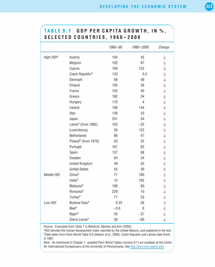
D E V E L O P I N G T H E E C O N O M I C S Y S T E M 323
T A B L E 9 . 1 G D P P E R C A P I T A G R O W T H , I N % ,S E L E C T E D C O U N T R I E S , 1 9 6 0 – 2 0 0 0
1960–80 1980–2000 Change
High HDIa Austria 104 42 ⇓Belgium 102 67 ⇓Cyprus 160 122 ⇓Czech Republicb 133 0.5 ⇓Denmark 68 49 ⇓Finland 105 56 ⇓France 102 40 ⇓Greece 182 34 ⇓Hungary 170 4 ⇓Ireland 106 144 ⇑Italy 126 43 ⇓Japan 241 54 ⇓Latviab (from 1965) 103 −22 ⇓Luxembourg 50 122 ⇑Netherlands 86 47 ⇓Polandb (from 1970) 50 25 ⇓Portugal 167 82 ⇓Spain 137 68 ⇓Sweden 64 34 ⇓United Kingdom 49 55 ⇑United States 55 56 ⇑
Middle HDI Chinab 71 180 ⇑Indiab 15 102 ⇑Malaysiab 168 85 ⇓Romaniab 229 10 ⇓Turkeyb 77 53 ⇓
Low HDI Burkina Fasob 0.22 26 ⇑Malib −0.6 6 ⇑Nigerb 35 −37 ⇓Sierra Leoneb 30 −60 ⇓
Source: Excerpted from Table 1 in Weisbrot, Naiman and Kim (2000).aHDI denotes the human development index reported by the United Nations, and explained in the text.bData taken from Penn World Table 5.6 (Heston et al., 2002). Czech Republic and Latvian data finishin 1997.Note: As mentioned in Chapter 1, updated Penn World Tables (version 6.1) are available at the Centerfor International Comparisons at the University of Pennsylvania. See http://pwt.econ.upenn.edu/

324 T H E E C O N O M I C S Y S T E M
A broad cross-section of countries is included in Table 9.1 ranked in groupsaccording to their human development index (HDI) score in 2004. The HDI isbased not on income solely but also includes criteria including health, education,life expectancy, income, poverty levels and environmental quality.
The broad trend that emerges is there has been a slowdown in economic growth,measured as GDP per capital internationally over the periods 1960 to 1980 and 1980to 2000. The first period includes the ‘Golden Age’ period between 1950 and 1973following World War Two and prior to the first oil-price shock when economiesinternationally, particularly the industrialized countries, expanded substantially.A minority of countries (highlighted in italics in Table 9.1) experienced highergrowth in GDP per capita in the second period.
While real output per capita provides an indicator of living standards, anothermeasure – real output per person employed – provides information on the produc-tivity of an economy’s workforce. This measure is called labour productivity.
Labour productivity: the amount of real output, on average, produced by eachworker in the economy. It is computed as
Real outputWorkers employed
.
Measurement of labour productivity differs from living standards in terms of thedenominator used because living standards is computed as
Real outputPopulation
.
In 2003 Finland’s real output was approximately ¤137bn (quoted in 2000 prices)and the number of workers employed was 2 365 000 (see http://www.stat.fi for statistical information; figures for real GDP are taken from http://www.stat.fi/tk/tp/tasku/taskue kansantalous.html while numbers employ-ed is available at http://www.stat.fi/tk/tp/tasku/taskue tyoelama.html). Com-puting Finnish labour productivity yields a figure of ¤57 928. Comparing thisto 2002 when real output was ¤134.5bn (in 2000 prices) and 2 372 000 workerswere employed indicates that labour productivity was ¤56 703.
Repeating this exercise for 2001 gives rise to a figure of ¤55 555(¤131.5bn/2 367 000). Hence we can say that real labour productivity increased

D E V E L O P I N G T H E E C O N O M I C S Y S T E M 325
in this economy between 2001 and 2003. This means that each worker on averageincreased the quantity of goods/services they produced.
The corresponding figures for living standards can be computed usingfigures for population. The population figure for 2001 was 5 201 000 andfor 2002 (latest available data) was slightly higher at 5 213 000. Hence, livingstandards for each Finnish resident in 2002 were ¤25 801 and in 2001 were¤25 284 indicating a rise in living standards of 2.04%. Over the same periodthe rise in labour productivity was quite similar at 2.06%.
When labour productivity rises over time this means that output is growing at a fasterrate than the number of workers employed (the labour input). The importance oflabour productivity for economic growth is evident if we consider that increasedlabour productivity reflects an increase in the productive efficiency of an economy.An economy that is able to increase the real output of the average worker may bemaking more efficient use of available resources, using them in more productiveways. In terms of our discussion of the production possibility frontier (refer backto Chapter 1), an economy that increases its average labour productivity with nochange in the amount of available resources or technology over time experiencesefficiency that allows it to increase its output and move its production point closerto its PPF. This would represent an improvement in the technical efficiency of theeconomy as better ways of using the resources are put in place. If more and morefirms in an economy adopt the ‘best practice’ methods for producing their goodsand services, technical efficiency would improve.
Logically, any barriers to the dissemination of best practice methods haverepercussions for efficiency and it would be in the economy’s interest to eliminatesuch barriers where possible. Firms that are in industry or trade associations wherebythey visit each others’ premises or are in regular contact and are aware of how bestto produce their output are usually quick to implement and imitate improvementsintroduced by their peers, which has a positive impact on the firms and on theeconomy as labour productivity could also be expected to rise in an economy thatapplies improved technology.
In the 1970s and 1980s many international manufacturing companies tried toimitate the best practice production methods originating in Japan that allowedJapanese producers to become efficient and competitive in many consumer

326 T H E E C O N O M I C S Y S T E M
electronics products and in the car/automobile markets. Many firms in theUSA, and elsewhere, found it difficult to produce products that could competeon price and quality relative to the available Japanese alternatives. Some firmswent out of business, others attempted to adopt best practices, although thisproved difficult since the Japanese model of production had many culturalaspects not easily imitated in non-Japanese firms.
Alternatively, an economy that experiences rising labour productivity might beenjoying the results of an increase in its resources (of capital, for example) availableto each worker, allowing each worker to produce more. If the capital input expandsbecause firms invest more in new machinery and equipment, for example, the coun-try’s production possibility frontier moves outwards reflecting increases productivecapacity of the economy. Again a higher amount of output can be produced causedby the rise in capital resources. If capital increases with no change in the labourinput and output produced rises, once again labour productivity increases.
A complex mix of economic factors affect labour productivity and are, therefore,important in the context of economic growth. For example,
1. The income taxation structure within an economy can have significant impli-cations for individuals’ incentives to work as individuals will not necessarily bewilling to give up welfare payments if faced with poverty traps.
A poverty trap (also sometimes known as an unemployment trap) exists when theopportunity cost of moving from unemployment benefits to paid employmentdoes not exist. Unemployed workers are often entitled to various benefitsin addition to unemployment payments. These may include housing or rentallowances, reduced medical costs, food vouchers, etc. On taking up paidemployment, especially of a low-paid nature, the benefits foregone may begreater than the wages earned. A vicious circle of poverty can be created whichis difficult to break.
2. Women (and men) who opt to take care of children and not work outsidethe home may not be enticed into the workforce unless sufficient incentivesexist to compensate them for childcare costs so that even if more employ-ees are in demand by firms, they cannot attract additional workers withoutincreasing wages.
3. High taxes on firms’ profits affect the location decisions of multinational firmsand high employers’ taxes reduce their incentives to increase their workforce.

D E V E L O P I N G T H E E C O N O M I C S Y S T E M 327
4. If a government attempts to attract firms via capital grants and/or the provisionof buildings they essentially change the relative prices of capital and labourmaking capital relatively cheaper which again impacts firms’ incentives toincrease employment.
5. The ease and availability of finance for investment matters for investmentpurposes. Overall business confidence in an economy in terms of favourableexpectations of future demand and economic developments feeds into firms’decisions regarding how much to invest in capital and research and developmentwhich ultimately contributes to economic growth.
The myriad of factors that affect economic growth (not exhausted above) impliesthat it can be extremely difficult to attempt to address the problem of slow economicgrowth. Given the relationship between living standards and labour productivity,however, adopting a perspective of economic growth based on improving labourproductivity through a more efficient use of resources is central.
9.2.1 THE DEPENDENCY RATIOUnfortunately labour productivity improvements do not necessarily or immediatelylead to higher living standards because the dependency ratio must be taken intoan account.
A country’s dependency ratio is the portion of the population not in employment(including the unemployed, those who have retired and children) relative tothe total population in employment. The percentage of employed people in thepopulation is known as the participation rate. Dependents are also often classifiedas ‘non-economically active’ as they are considered to consume but not produceeconomic outputs.
Table 9.2 provides information relating to 2001 on dependency ratios for a selectionof countries.
For Austria 16.5% of its population is between 0 and 14 years of age, 11.8% isin the segment between 15 and 24, etc. The dependency ratio is the sum ofthe shares of the non-economically active segments (defined as children up to14 years and those of 65 years and older) stated as a percentage of the rest ofthe population (those between 15 and 64 years).

328 T H E E C O N O M I C S Y S T E M
T A B L E 9 . 2 I N T E R N A T I O N A L D E P E N D E N C YR A T I O S A N D P O P U L A T I O N S H A R E S , 2 0 0 1
Dependency 0–14 15–24 25–64ratio years years years 65+
Austria 47.2 16.5 11.8 56.1 15.5
Belgium 52.5 17.6 12.1 53.5 16.9
Chinaa 46.4 36.4 – – 10.0
Cyprus 51.8 22.7 15.4 50.5 11.4
Czech Republic 43.7 16.1 14.8 53.5 13.8
Denmark 50.3 18.7 11.2 55.3 14.8
Estonia 49.0 17.6 14.7 52.4 15.3
Finland 49.4 18.0 12.7 54.3 15.1
France 53.8 18.8 13.0 52.0 16.2
Germany 47.7 15.4 11.3 56.4 16.9
Greece 47.9 15.3 14.1 53.5 17.1
Hungary 46.4 16.5 14.3 54.0 15.2
Indiaa 62.5 54.4 – – 8.1
Ireland 53.7 21.4 17.2 43.4 11.2
Italy 48.4 14.4 11.4 56.0 18.2
Japan 46.8 21.6 – – 25.2
Latvia 47.9 17.0 14.6 53.0 15.4
Lithuania 50.2 19.3 14.5 52.1 14.1
Luxembourg 48.8 18.8 11.5 55.7 14.0
Netherlands 47.2 18.0 11.9 56.1 14.1
Poland 44.8 18.5 17.0 52.1 12.4
Portugal 48.1 16.0 14.2 53.4 16.5
Slovakia 44.0 19.0 16.9 52.2 11.4
Slovenia 42.6 15.6 14.3 55.8 14.3
Spain 46.2 14.6 13.8 54.6 17.0
Sweden 55.0 18.3 11.6 52.9 17.2
United Kingdom 52.8 18.9 12.1 53.3 15.6
United States 50.6 21.2 14.0 52.4 12.4
Sources: Data compiled from United Nations, 2003; except for countries marked a where data takenfrom United Nations, 2002.

D E V E L O P I N G T H E E C O N O M I C S Y S T E M 329
The percentage of each country’s population that falls into different age groupsis shown in Table 9.2.
The dependency ratio for Austria is 47.2 which is found by
1. summing up the share of the population between 0 and 14 (16.5%) andthe share over 65 (15.5%) = 32%;
2. summing up the economically active population between 15 and 64, i.e.11.8% + 56.1% = 67.9%;
3. expressing 32 as a percentage of 67.9 = 47.2%.
This dependency ratio implies that for every 100 people in the population, 47are dependents. Note these measures do not account for unemployment.
It is also possible to compute separate ‘young dependency’ and ‘elderly’ dependencyratios. Concern has been raised recently in industrialized countries about increasedlife expectancy (rising elderly dependency) and the pressure thus created onpension-systems. The proportion of the world’s population over 65 is predicted todouble by 2030, from about 8% to more than 16%. For members of the Organizationfor Economic Cooperation and Development the percentage is expected to risefrom 18% to 32% over the same period. Coupled with falling fertility rates thismeans smaller populations will have to support greater shares of non-economicallyactive people.
Fertility rate: the number of children born in a year, usually expressed per 1000women in the reproductive age group.
In 1970 average international fertility rates were 3.33; currently they are 2.96and are expected to drop to 2.5 by 2020. In fact Ireland had the distinctionin the 1990s of being the sole European country where the fertility rate wassufficiently high to lead to a rise in the overall population – in all other Euro-pean countries populations were declining as the fertility rate was less than thereplacement rate, i.e. that required to replace deaths.
These international trends create challenges that will have to be faced by govern-ments, pensions-administrators and by workers in the not too distant future. (Formore on the pensions debate see Cato, 1998.)

330 T H E E C O N O M I C S Y S T E M
The importance of the dependency ratio for understanding trends in labourproductivity and living standards can be considered using an example.
Before the 1990s in Ireland, labour productivity growth did not translateinto proportional growth in living standards because of high levels of unem-ployment and dependency. However, during the 1990s growth in labourproductivity eventually coincided with improved living standards because itreflected a more efficient use of resources and allowed Irish goods and servicesto become more competitive relative to those produced elsewhere. Up to thelate 1980s high Irish unemployment reflected general international recessionsand the inability of many inefficient Irish producers to compete either domes-tically or internationally. By the mid 1990s the ‘Celtic Tiger’ had emerged (areference to the name often used to denote the four Asian Tiger economiesof Hong Kong, Singapore, Taiwan, and South Korea that achieved relativelyhigh rates of growth over the 1960s to the mid-1990s) and rising employmentmeant that growth in productivity translated into living standards figures also,as shown in Table 9.3.
Table 9.3 shows that real output of the Irish economy accelerated from 1993onwards at 8.3% on average each year to 2000. To explain this jump we seethat from 1993 annual growth in employment also increased substantially to
T A B L E 9 . 3 E C O N O M I C G R O W T H , P R O D U C T I V I T Y A N DE M P L O Y M E N T
Annual average growth rates %
Living standards, i.e. Productivity, i.e.Period GDP Population Employment GDP/capita GDP/worker
1960–1980 4.1 0.9 0.5 3.1 3.5
1980–1993 3.3 0.4 0.0 2.9 3.3
1993–2000 8.3 0.8 4.7 7.4 3.5
Source: Kennedy, 2001. Data taken from Irish National Income and Expenditure, various issues; ESRI Quarterly EconomicCommentary, December 2000; and Kennedy, K. (1971) Productivity and Industrial Growth: The Irish experience. ClarendonPress, Oxford.

D E V E L O P I N G T H E E C O N O M I C S Y S T E M 331
4.7%. Living standards too jumped dramatically from 1993 onwards. Althoughthe growth in labour productivity was almost stable since 1960, becauseincreasing numbers of people could find work since 1993, the overall outputof the economy increased substantially. The dependency ratio fell as theunemployment rate dropped from 15.5% in 1993 to 4.2% in 2000. The gapbetween the population and the employed population explains why growthin living standards was below that for productivity until the period beginning1993. As employment increased this gap closed, allowing living standardsto grow faster than productivity and allowing a greater proportion of thepopulation to share in the economic growth through their new-found jobs.
9 . 3 E C O N O M I C G R O W T H O V E R T I M EEconomies are not static entities. The ceteris paribus assumption helps economiststheorize about the economy and facilitates their analyses of the economy butfactors do not remain constant for very long. Economic decisions are made, goodsand services are bought and sold, demand conditions change, supply conditionschange, population and unemployment rise and fall, real output is produced andreal income is earned and spent. Ideally economies should expand or grow overtime meaning more real output is produced. The more output produced, the moreincome generated for the citizens of a country. We all probably hope that ourchildren and grandchildren will be materially (and non-materially) better off thanourselves, which implies that there will be more real output/income generatedby their economies to be shared among the population. Table 9.1 indicates quitedifferent outcomes across various countries in terms of their growth experiences asrevealed by average living standards internationally over the last 40 years.
The rate at which an economy grows matters if we consider what happens to realincome if long-run growth is 3% each year. Real national output for Ireland in 1978was IR£15 815m (expressed in 1995 prices). We can compute how long it wouldtake for real income to double (to £31 630m) assuming a growth rate of 3%. Thefollowing formula applies:
Future value = initial value (1 + growth rate)n; where n denotes time period
(i) To compute n rearrange the above:
Future value (FV )
Initial value (IV )= (1 + growth rate (GR))n

332 T H E E C O N O M I C S Y S T E M
(ii) It is true that log (FV /IV ) = n log (1 + GR)
(iii) Dividing both sides by log (1 + GR) gives log (FV /IV )/log (1 + GR) = n(iv) To compute GR rearrange the above:
Future value (FV )
Initial value (IV )= (1 + growth rate (GR))n
(v) This can be rearranged as (FV /IV )1/n = (1 + GR)
(vi) Finally GR can be found as [(FV /IV )1/n] − 1 = GR
Applying the formula to this example:
(i) £31 630m/£15 815m = (1 + 0.03)n : 2 = (1.03)n
(ii) log (2) = n log (1.03)(iii) log (2)/log (1.03) = 0.301/0.013 = 23.15
This means that it would take 23.15 years for real output to double assumingthe above information holds. What we would find for a lower growth rate of say1.5% (half of 3%) is that it would take twice as long – over 46 years – for outputto double. This indicates that the rate of economic growth really matters foreconomies, for their real output and hence for living standards.
In actual fact 23 years after 1978, in 2001, Irish real output was £67 615,more than trebling over the period. This implies a substantially higher rate ofgrowth than 3%. We can compute what the growth rate was again using theabove formula. This time the future value is £67 615m and the variable we wishto compute is the growth rate (GR). (For simplicity the time period used is 23years rather than 23.15.)
(v) (£67 615m/£15 815m)1/23 = (1 + GR) = 4.281/23 = (1 + GR)
(vi) 1.0653 = (1 + GR) = 1.0653 − 1 = 0.0653
A growth rate of over 6.5% corresponds to the observed real growth in Irishoutput between 1978 and 2001. This figure of 6.5% is an average computedover the entire period but in fact, as Table 9.3 showed earlier, real Irish outputgrew mostly after 1993.
To understand the processes underlying economic growth Solow’s growth model isconsidered further in the sections that follow.

D E V E L O P I N G T H E E C O N O M I C S Y S T E M 333
9 . 4 M O D E L L I N G E C O N O M I C G R O W T H :T H E S O L O W G R O W T H M O D E L
In 1956, Robert Solow, who received the Nobel Prize in Economics in 1987,developed a model of economic growth that focuses on long-run economic growthand its determinants, as opposed to the short-run fluctuations we considered earlierin the discussion of the business cycle. (This approach to modelling economicgrowth is also called the neoclassical growth model.) Long-run growth is related tothe production possibilities or productive capacity of an economy, which usuallychange very little over short periods of time but which can change over longerperiods. In terms of the tools we have already met, economic growth correspondsto an outward expansion of the production possibilities frontier or a rightward shiftof the aggregate supply curve.
Solow’s growth model uses the production function approach discussed inChapter 5 (see section 5.8). The production function summarizes the relationshipbetween the factors of production (K and L), the level of technology (T), andoutput (Y ), as:
Y = F (K, L, T )
From this relationship, any change in the quantity or quality of the productive factorsor technology has an impact on the level of output the economy can produce.
Just how changes in K or L actually affect Y (e.g. Y increasing by 5% if L risesby 10%) is not covered in this text but would be described in a more specificproduction function than the general function presented here as Y = F (K, L, T ).
One example of a more specific functional relationship between Y , K , L and Twould be Y = T × (K α) × (Lβ) with values provided for T , α and β (these valuescould be estimated from analysis of available economic data).
Where the value of α plus β is less than 1, e.g. 0.3 and 0.5 (summing to 0.8), itwould imply that decreasing returns to scale describe the relationship between thefactors of production and output – if inputs both doubled, output would rise but byless than double. If α plus β sum to greater than 1, increasing returns to scale aredescribed (output rising faster than a joint input rise) and if they sum exactly to 1,constant returns to scale apply to the economy.
Relating the production function to our discussion of labour productivity (andassuming that resources are used efficiently) any change in labour productivity is

334 T H E E C O N O M I C S Y S T E M
due to either a change in the quality or quantity of capital available to each workeror to a change in available technology.
In the Solow model, technology is assumed not to be influenced by K and Limplying that changes in the capital stock, K , or labour input L do not affecttechnological progress. In other words, technology is assumed to be exogenous to theSolow model as it is determined outside the model itself and not influenced by othervariables in the model: technological change just happens without explanation. (Anumber of economists have examined this exogeneity assumption with interestingresults but before discussing these it is necessary to initially consider the Solowmodel and its implications).
Figure 9.1 presents an illustration of a production function. To draw the produc-tion function in two dimensions – here we use output and capital – we assume thatthe production function is drawn for one given level of technology and for a givenlevel of labour supply. This allows us to focus on how output is related to the capitalinput, given T and L.
The production function indicates the amount of output produced for differentlevels of capital input (given T and L). We see that long-run output depends on thelevel of the capital stock in the economy. If the level of capital stock is K1, outputis Y1; when it is K2, output is Y2. Furthermore, for any two economies with similarproduction functions if the level of capital in one country is K1 while it is K2 in theother country, the output levels in both countries will differ substantially.
We also see that output rises as the stock of capital employed increases butthe relationship is nonlinear. This implies that output does not rise by a constant
Output: Y
Capital: K
Productionfunction
K1 K2
Y1
Y2
K3
Y3
F I G U R E 9 . 1 P R O D U C T I O N F U N C T I O N I N T H E S O L O WG R O W T H M O D E L

D E V E L O P I N G T H E E C O N O M I C S Y S T E M 335
amount if the capital stock changes. For example as the capital stock rises fromzero to K1, output rises relatively sharply from zero to Y1. As the capital stockrises further from K1 to K3 (an increase of roughly 200% here), output alsorises but by a smaller proportion – approximately 50%. This nonlinearity illustratesdiminishing returns to capital. For a given number of workers, adding more andmore capital contributes ever declining amounts to total output. The initial benefitof doubling capital when the capital stock is low allows workers to increase theiroutput substantially. Doubling capital when the capital stock is high and eachworker already has a lot of capital with which to work generates lower additionalincreases in total output.
Since the level of output in the long run depends on the level of capital stock,any change in the capital stock causes a change in output. If an economy has a levelof output at Y1 and wishes to expand output to Y2, investment in more capital stockis required. Such investment is undertaken by both firms and governments; firmsmake private investments that change the stock of private capital and governmentsengage in public investment that change the amount of public capital.
To increase the capital stock investment in new capital must be sufficient to morethan cover any depreciation that normally occurs as capital is used for productivepurposes. Once capital investment is greater than depreciation the capital stockrises and so too does output (assuming that the output is in demand!). If investmentis less than depreciation, an economy experiences a decline in its capital stock andin output. If investment just covers or offsets the capital lost due to depreciation,the levels of capital stock and output remain constant or unchanging. Solow calledthis case the steady state.
At any level of investment, either above or below the level required to coverdepreciation in the economy, the economy is not at its steady-state level of outputand the capital stock will either rise or fall with knock-on effects on the levelof output.
The steady state is the term used by Solow to describe the equilibrium state ofoutput and capital stock in the long run. (The term is also used in physics.) Aneconomy that reaches a steady-state level of capital stock and level of output hasno tendency to change from these levels, ceteris paribus.
Figure 9.1 can be extended to consider investment and depreciation further. Havingdiscussed investment in Chapter 5, we know that expectations play a key role infirms’ determination of their investment levels. Predicted future demand is centralto the investment decision.

336 T H E E C O N O M I C S Y S T E M
Many factors enter into governments’ decisions regarding public investment butit is closely related to the level of development of the economy – classified as low,medium or high – and to the government’s policy goals. It may take the form of hardinvestments in physical infrastructure or soft investments including services, educationor technology.
If we consider that national savings is the main source of actual investment fundswe can describe actual investment as equal to national savings, which itself is afraction of national income (equating investment with national savings is strictlytrue only if there is no government expenditure or trade). Including governmentand foreign sectors implies:
Investment = savings − government deficit (or + government surplus)
+ foreign financing.
If Y denotes national income then savings or the funds for investment is a fractionof Y . If the fraction of Y saved were 25% we can add this as the savings = actualinvestment function shown in Figure 9.2.
To include depreciation in the diagram, it is assumed that a constant fractionof the capital stock requires replacement annually as it becomes obsolete. If thisfraction is 20% then 20% of K depreciates each year and will be written off inthe national accounts; if no investment takes place the capital stock declines. It isreflected in Figure 9.2 by a straight line with a slope of 0.20. The linear relationshipbetween depreciation and capital stock implies that for any change in capital stock,depreciation will always be 20% of this change (so if the level of K is 10, depreciationis 2).
Output/depreciation/investment
Capital: K
Productionfunction
K1 K2
Y1
Y2
Savings = actualinvestment
Depreciation
K*
Y*
F I G U R E 9 . 2 S O L O W G R O W T H M O D E L W I T H I N V E S T M E N TA N D D E P R E C I A T I O N

D E V E L O P I N G T H E E C O N O M I C S Y S T E M 337
In Figure 9.2, K ∗ denotes the level of the capital stock required for investment tojust cover depreciation. This is the steady-state level of capital stock, the only levelfrom which the economy has no tendency to change, ceteris paribus. At other levels ofcapital stock, this is not the case. If K1 is the level of capital stock and Y1 the outputof the economy, investment is greater than depreciation and the tendency is for thecapital stock to rise with an impact on output also. For levels of capital stock aboveK ∗ such as K2, depreciation is above investment, and investment is insufficient toreplace depreciating capital stock, hence the tendency is for the capital stock levelto decline and, therefore, for output to fall. Whenever the level of the capital stockis not at K ∗, it tends to move towards K ∗.
The steady-state level of capital stock K ∗ corresponds to a level of output of Y ∗
on the production function.Another implication of the production function drawn here is that of conver-
gence.
Convergence is the tendency for poorer countries to grow faster than richercountries for a given increase in capital stock. Hence, poorer countries wouldbe expected to catch up with richer countries if the countries share similarsteady states.
Richer countries (i.e. those with higher per capita income levels) have higher levelsof capital stock than poorer countries. Given the assumption of diminishing returnsto capital, this implies that for any increase in the capital stock the additional outputproduced from the capital will be lower in the richer country than the poorercountry starting from a lower level of capital stock and lower level of income. Theproductivity of capital will be higher in the poorer country. Historically, followingWorld War Two, Japan and Germany invested heavily in renewing and improvingtheir capital stock relative to the USA and UK and this is one of the factors thatis considered to explain their relatively better productivity. Similar arguments areused to explain the Asian Tiger phenomenon.
9.4.1 MORE ON SAVINGSSavings rates for many countries are published on a regular basis. A recent report bythe Organization for Economic Cooperation and Development (OECD) providedthe information presented in Table 9.4 on household saving rates across a range ofindustrialized countries. Countries’ ranking are presented in the final column whilean indication of the general trend is shown in the second-last column of the table.The predominant trend in household saving has been a decline. In some countries,

338 T H E E C O N O M I C S Y S T E M
T A B L E 9 . 4 I N T E R N A T I O N A L H O U S E H O L DS A V I N G S R A T E S
Country 1985 1990 1995 2000 2002a Change Rank ’02
Australia 10.8 9.3 4.8 3.4 0.3 ↓ 19
Austria 10.5 14.0 11.7 8.3 7.5 ↓ 12
Belgium 15.9 18.0 18.8 13.4 13.7 ≈ 2
Canada 15.8 13.0 9.2 4.8 4.4 ↓ 17
Czech Republic – b – 20.6 13 11.3 ↓ 5
Denmark – 11.2 6.9 4.8 6.2 ↓ 14
Finland 3.4 2.2 5.2 −0.9 −0.3 ↓ 20
France 8.9 7.8 11.2 10.8 12.2 ≈ 3
Germany 12.1 13.9 11.2 9.8 10.4 ↓ 7
Ireland 10.6 6.5 8.5 6.0 7.5 ↓ 12
Italy 30.7 27.8 22.5 14.5 16.0 ↓ 1
Japan 16.5 14.0 11.9 9.8 5.8 ↓ 15
Korea 14.8 22.0 16.8 11.5 9.6 ↓ 9
Netherlands 5.6 11.6 14.9 6.7 10.7 ↑ 6
New Zealand – 0.5 −3.6 −3.8 −0.3 ≈ 20
Norway −3.3 0.8 4.6 4.5 7.0 ↑ 13
Portugal – – 13.6 9.5 11.9 ↓ 4
Spain 11.1 12.3 14.4 10.6 10.1 ↓ 8
Sweden 3.2 0.0 8.3 2.4 8.2 ↑ 11
Switzerland – 8.7 9.4 8.3 9.0 ≈ 10
United Kingdom 9.8 8.0 10.0 4.3 5.2 ↓ 16
United States 9.2 7.8 5.6 2.8 3.7 ↓ 18
Source: OECD, 2002Notes: a 2002 figures are projections.
b Data unavailable.

D E V E L O P I N G T H E E C O N O M I C S Y S T E M 339
the decline has been dramatic – Australia, Canada, Italy (from a very high share),Japan, the USA, and the UK.
There are many possible reasons why the savings rate varies a lot across countries.Different demographic patterns between countries lead to different savings rates ascountries with a high proportion of the population in older age groups tend to havehigher savings rates. National tax policies affect people’s saving/consumption incen-tives and decisions. Cultural differences also play a role, as does the level of develop-ment, and political and economic stability. Savings rates tend to be highest in coun-tries with high income-levels, which could mean also that high income promoteshigh rates of saving. Economists have not identified which of the many possibleexplanations is most important to explain international differences in savings rates.
The Solow model can be used to consider what happens if a country’s savingsrate changes. A decision to increase the proportion of income saved, for example,moves the savings = actual investment function up, as shown in Figure 9.3.
With the higher savings rate, at any level of capital stock the amount of investmentis higher, so the new savings function 2 lies above the initial function. We canconsider the implications of this change beginning at the initial steady state. Usingsavings function 2, we see that at K ∗, savings = actual investment lies above thedepreciation line. This means there is a tendency for the economy to move fromits steady state and the capital stock rises due to increased net investment. In fact,the capital stock increases until K2 is reached (where the new savings functionintersects the depreciation line and where savings = actual investment just coverscapital depreciation). The higher capital stock of K2 denotes a new steady stateinvolving both higher capital stock and higher output.
Governments sometimes intervene to affect savings. Remember consumershave the options to either save or spend on consumption goods. High levels
Output/depreciation/investment
Capital: K
PF1
K1 K2
Y1
Y2
Savings 1
Depreciation
K*
Savings 2
F I G U R E 9 . 3 I N C R E A S E I N T H E S A V I N G S R A T E

340 T H E E C O N O M I C S Y S T E M
of consumption correspond to low levels of saving. High levels of aggregate demandcorrespond to booms and to encourage consumers to change their savings behaviourgovernment might be anxious to try to reduce aggregate demand (if inflation orinflation expectations were rising, for example). Or to encourage greater savingsfor pensions, governments often offer tax concessions as an incentive to changesavings behaviour. But is there an ideal or optimal savings rate for an economy?
Imagine that consumers wish to maximize their consumption out of the incomegenerated in their economy and income is either consumed or saved (i.e. usedfor investment). There are, in fact, unique levels of capital stock (K ∗) and output(Y ∗) that correspond to maximizing consumption, which are shown graphically inFigure 9.4.
The production function indicates the maximum levels of consumption possibleif no income/output is diverted for savings/investment (and if no taxes werediverted to government and if no external trade occurred!). Even if no incomeis saved a certain amount of capital depreciates each year, reducing the amountof income available for consumption. For Figure 9.4 panel A we can consider justby looking at the graph where the biggest difference exists between output anddepreciation; this indicates the unique values of output (Y ∗) and capital stock (K ∗)at which consumption would be maximized. The intuition behind this result is thatonly at these points is the marginal return to capital (the slope of the productionfunction) the same as the rate of depreciation. At any higher (lower) capital stock
Output/depreciation
Capital: K
Productionfunction
Depreciation
K*
Y*
Output/depreciation
Capital: K
Productionfunction
Depreciation
K*GRGolden rule level of capital
Y*
Savings
A B
F I G U R E 9 . 4 S O L O W G R O W T H M O D E L : S A V I N G S A N DC O N S U M P T I O N

D E V E L O P I N G T H E E C O N O M I C S Y S T E M 341
the rate of deprecation would be greater (less) than the return of the capital in theeconomy. Only at these points is there no incentive to change the capital stock.
In Figure 9.4 panel B a savings function is added. The golden rule level of capital(K∗GR) corresponds to the point where depreciation = savings and consumption ismaximized. This outcome is far from certain for an economy. One unique savingsfunction must apply, as shown in Figure 9.4 panel B. For any other savings function,the optimum level of consumption does not occur and the level of capital stockdiffers from K∗GR.
9.4.2 THE SOLOW MODEL AND CHANGES IN LABOUR INPUTUsing the Solow model to examine the impact of changes in labour on outputand economic growth is complicated. Why? Because using the production functionapproach we assumed T and L are fixed. Relaxing this assumption for a while, takethe case where the labour input increases and we assume the economy is initiallyoperating efficiently. With a rise in quantity of the labour input (L) only and nochange in capital, each worker (on average) has less capital with which to work. Thenet effect on output depends on the relative effects of
1. lower average productivity due to the drop in capital per worker;2. rising total output produced by the extra workers.
See the box for examples.
An economy produces output efficiently. It has 100 workers and average pro-ductivity is 10 baskets of output. Therefore, national output is 100 × 10 = 1 000.
Example 1
Labour rises by 5% to 105 workers. Capital does not change. Each worker hasless capital and so their productivity declines by 10% to 9 baskets. New nationaloutput is 105 × 9 = 945. This represents a drop of 5.5%.
Example 2
Labour rises by 10% to 110 workers. Capital does not change. Each workerhas less capital and so their productivity declines by 5% to 9.5 baskets. Newnational output is 110 × 9.5 = 1045. This represents a rise of 4.5%.

342 T H E E C O N O M I C S Y S T E M
Thus, the impact on output depends on the precise relationship between output,capital, labour and technology for the economy at that point in time, i.e. itsproduction function!
There is a further possibility. It could be envisaged that an increase in the labourinput could occur either if more workers become available or if the quality of theworkforce improves (due to better education or skills, for example). In such a case,greater numbers of more efficient or productive workers might reduce or evencancel out the effect of having less capital with which to work. All of this impliesthat it is difficult to predict exactly what the effect of changes in the labour forcewill have on real output.
If the quantity of workers and capital are both increasing, however, the Solowmodel is useful for considering the effects of increasing labour inputs for outputand economic growth. A rising labour input reduces capital per worker (as withdepreciation). In order to maintain a constant amount of capital for each workerin the economy if the labour input is rising, investment must cover not onlydepreciation but also the capital required to supply all new workers with capital:capital widening is required.
In an economy where the capital stock increases at the same rate as the labourforce and covers depreciation, capital widening occurs.Capital deepening occurs when the capital stock increases faster than the labourforce so that the amount of capital per worker rises.
At the level of the macroeconomy, if capital widening occurs, a given level of capitalper worker (K1 for example) can be maintained, which is associated with a specificlevel of output (Y1). To maintain Y1 if the labour input is rising requires greaterinvestment than if labour is unchanging.
Capital deepening would be funded through savings leading to higher investment.In an economy with a workforce growing by 5% each year, for example, investmentwould have to grow by 5% just to keep a constant amount of capital available to eachworker. This is apart from the investment required to replace depreciating capital.If our economy above experiences 20% depreciation and 5% labour force growththen investment to the value of 25% of the capital stock is required to maintain aconstant level of capital stock per worker.
A rise in labour coupled with capital deepening would lead to a further expansionof the production function. In an economy where constant returns to scale prevail,output grows at the same rate as input growth. In other words if both capital andlabour increase by 5% then output grows by 5% also, reflected in an upward shiftof the production function.

D E V E L O P I N G T H E E C O N O M I C S Y S T E M 343
In measuring the changes in labour input, economists usually use averageannual hours worked in an economy, which is estimated based on broad surveysof companies usually carried out by national statistical agencies. This measure oflabour input is preferred to a measure of the number of workers because of thechanging patterns of work for many individuals. Focusing solely on the numbersof workers employed reveals that numbers employed internationally have risen(this is true using historical data going back to 1870) but since part-time work isquite commonplace and given labour policies and regulations, hours worked perperson have actually fallen internationally.
9.4.3 THE SOLOW MODEL AND CHANGES IN TECHNOLOGYThe Solow model assumes a given level of technology. Allowing technology toimprove, ceteris paribus, allows more output to be produced from a given amount ofinputs. This means the production function moves up as shown in Figure 9.5.
An economy with an amount K1 of capital can increase its output from Y2 to Y1given better technology. If the economy begins with K2 capital its output increasesfrom Y3 to Y4. The country with the higher initial capital stock experiencesa greater absolute rise in output. We can extend this figure to illustrate thattechnology improvement is a more important source of growth than increasedcapital for more industrialized countries, ceteris paribus.
This case is shown in Figure 9.6. Imagine two countries with production functionslike PF1 that both experience technology improvements allowing their productionfunctions to move to PF2. One country is relatively poor with a low capital stock ofK1; the second country has a higher capital stock of K2. Both countries experiencethe same absolute increase in capital stock.
Output
Capital: K
PF1
K1 K2
Y1
PF2
Y2
Y3
Y4
F I G U R E 9 . 5 I M P R O V E D T E C H N O L O G Y

344 T H E E C O N O M I C S Y S T E M
Output
Capital: K
PF1
K1 K1
Y1
PF2
Y1*
Y2
Y2*
Higher capital stock explainsa portion of increased output
Improved technology explainsa portion of increased output
K1* K2*
F I G U R E 9 . 6 I M P R O V E D T E C H N O L O G Y : R I C H V S .P O O R C O U N T R I E S
K1 rises to K1∗ as shown in Figure 9.6 while K2 rises to K2∗. Since the marginalproduct of capital is higher for the poorer country with the lower stock of capital,the expansion of its capital stock is responsible for approximately half of its increasein output from Y1 to Y1∗. Compare this to the rise in output for the richer country.Because the production function is relatively flatter for the richer country since itscapital stock is higher, most of the expansion in its output from Y2 to Y2∗ is causedby the shift in the production function.
This implies that developing or non-industrialized countries benefit more fromincreasing their capital stock than do more advanced economies. Advancedeconomies can expand their output but technology improvements are a relativelymore important source of their growth.
9.4.4 EXPLAINING GROWTH: LABOUR, CAPITAL AND TECHNOLOGYAny change in national output can be explained by changes in capital or labour ortechnology. More specifically a technique known as growth accounting categorizesthe separate sources of output changes.
Growth accounting is a method of identifying the proximate causes of changesin output and its rate of growth. The main causes are:
1. The marginal product of capital – linked to where on the production functionan economy produces, ultimately explained by past investment decisionsinfluencing the capital stock.

D E V E L O P I N G T H E E C O N O M I C S Y S T E M 345
2. The amount of capital in use.3. The marginal product of labour.4. The amount of labour in use5. Total factor productivity – a measure of the efficiency with which inputs are
employed to produce output. TFP is a catch-all term that measures theeffect on output not only of any changes in technology, but also in thesocial and political systems that affect the quantity and quality of outputthat an economy can produce from its labour and capital resources. TFP iseffectively that portion of output change that cannot be accounted for bychanges in the quantity and quality of labour and capital.
Any change in output not accounted for by changes in capital accumulation orchanges in labour input is called total factor productivity (TFP). It is also known asthe Solow residual – growth left unexplained after inputs have been accounted for.
The extent to which differences in the quality and quantity of inputs explaindifferences in productivity across countries is shown in Table 9.5. The first columnindicates each country’s labour productivity expressed as a percentage of that of theUnited States. The other columns present counterfactual analysis, best interpretedby taking an example. Australia’s output was measured as 83% of that of the USA. IfAustralia’s labour and TFP were the same as in the USA, with capital being the onlydifferent factor, its labour productivity would have been 109% of that in the USA.This implies greater relative capital productivity in Australia but since its output isless than the USA, differences in its other input (labour) and/or TFP reduce itsoverall relative productivity performance.
9.4.5 CONCLUSIONS FROM THE SOLOW MODEL
• The level of output is determined by the amount of capital in an economy, givenlabour and technology. This supports the general observation that countrieswith substantial capital investments (per worker) have relatively high levels ofoutput and productivity.
• The long-run equilibrium level of output and capital depends on the savingsrate of an economy. In equilibrium the level of capital (and output) is constant.Investment is sufficient to cover depreciation and any growth in the labourforce. International evidence indicates high correlations between savings ratesand living standards (e.g. Summers and Heston, 1991).
• An increased savings rate leads to a new equilibrium with higher capitalinvestment and higher output level. A higher savings rate leads to economicgrowth temporarily until the new equilibrium is reached.

346 T H E E C O N O M I C S Y S T E M
T A B L E 9 . 5 S O U R C E S O F I N T E R N A T I O N A LP R O D U C T I V I T Y D I F F E R E N C E S
Output per workerCountry as % of US output Capital Labour TFP
Australia 83 109 90 86
Austria 71 108 67 98
Belgium 84 102 84 98
Canada 94 100 91 103
China 6 89 63 11
Czechoslovakia 21 115 76 24
Denmark 69 108 91 71
Finland 73 120 86 73
France 82 109 67 113
Germany (west) 82 112 80 91
Greece 47 102 68 67
Hungary 31 112 93 29
India 9 71 45 27
Ireland 58 105 77 71
Italy 83 106 65 121
Japan 59 112 80 66
Korea 38 86 76 58
Netherlands 81 106 80 95
New Zealand 72 112 102 63
Norway 76 120 91 70
Portugal 37 96 50 76
Spain 68 102 61 111
Sweden 79 103 85 90
Switzerland 87 119 83 88
United Kingdom 73 89 81 101
Source: Excerpted from ‘Data Appendix’ for Hall and Jones (1999).

D E V E L O P I N G T H E E C O N O M I C S Y S T E M 347
Hence, high savings rates do not generate persistent economic growth.
• Growth in the population or labour force matters for living standards. Witha growing labour force, ceteris paribus, labour productivity falls. Correlationsindicate that countries with fast rates of population growth experience relativelylower levels of living standards.
• In the steady state, growth can only occur via TFP changes.
The Solow model does not deal with causes of technology improvement sincetechnology is exogenous or not explained within the growth model itself. We canallow technology to become an endogenous factor and such endogenous growthmodels are considered in section 9.4.6, which follows.
The conclusions do not help us understand why some countries do not experienceconvergence of income levels. We need to look elsewhere to understand thisphenomenon. Nor do we have an indication of welfare implications of economicgrowth, which is also examined in section 9.5.
9.4.6 ENDOGENOUS GROWTHEndogenous or new growth models essentially try to explain how and why changesin technology occur. Technology is not assumed to be unchanging and the result ofthings occurring outside the models. Some endogenous growth models discard theassumption of diminishing marginal product of capital so that a change in capitalleads to a constant proportional increase in output irrespective of the initial levelof capital stock. This implies a rising but linear production function, as shown inFigure 9.7. This means that every one-unit increase in the capital stock increasesoutput by the same amount, irrespective of an economy’s initial level of capital stock.
Adding our assumption about savings being a constant proportion of output, wedraw a corresponding savings function, which is also linear. By further including thedepreciation line, we complete the essential elements of the model. By definitionthe steady state occurs where there is no tendency to change from one level ofthe capital stock. But in Figure 9.7 no such point exists. Investment lies abovedepreciation indicating that the level of capital stock can rise indefinitely withoutany technological change, allowing output to rise also.
Another interesting result from the model occurs with an increase in the savingsfunction. If people’s savings behaviour changes so that savings increase and thesavings function moves up, the result is an increase in the economy’s stock of capitaland in its rate of output growth – the production function also moves up indicating

348 T H E E C O N O M I C S Y S T E M
Output
Capital: K
PPF
Depreciation
Savings
F I G U R E 9 . 7 P R O D U C T I O N F U N C T I O N W I T H C O N S T A N TM A R G I N A L P R O D U C T
a positive link between savings and a permanent rise in output growth (a new steeperslope of the new PPF indicates a change in the rate of growth).
A key issue arises as to the credibility of assuming a constant marginal productof capital. This may be possible if we allow investment to have an impact onthe quality of labour, and vice versa. The greater the amount of physical capital(buildings, equipment, machines, etc.) in an economy, the greater the output thathuman capital (skills, education, etc.) can produce and the higher the return onfurther investment to improving education and skills to maximize the productivityof physical capital. Each separate component of capital may exhibit diminishingmarginal product but in combination, they could give rise to a constant marginalproduct of combined, or total, capital. Poorer countries with not only low levelsof physical capital, but also of human capital, face a double disadvantage in tryingto catch up. Not only is investment in physical capital required but spendingon training and education is also required and by its nature the return on suchinvestments takes years to yield rewards. Many poorer countries with very limitedbudgets do not have the luxury of spending in the hope of generating future growthas the opportunity cost of such spending is considered too high. What is importantfor long-term growth is subordinated to urgent expenditures required today.
Growth benefits from investment may go beyond individual firms who undertakethe investment indicating that diminishing returns to capital may be relevant fora firm but not for society overall. Consider the effect on economic growth of autility company investing in providing broadband technology. The provider willdecide to invest in the broadband technology taking account of its own costs andpotential revenues. The provision of broadband technology, however, can increaseoutput and productivity of those firms that adopt it allowing them to increase their

D E V E L O P I N G T H E E C O N O M I C S Y S T E M 349
output for a set amount of inputs. The social benefit may outweigh the privatebenefit and create constant or even increasing returns to capital investment for theeconomy.
The potential for such a scenario creates challenges for government and whetheror not it should try to encourage capital investments by private firms that generateeconomy-wide benefits. Private firms usually do not take social benefits into accountin their investment decisions (and consider only their private costs and benefits) somaybe government should subsidize investments that give rise to broader economy-wide benefits? This sounds somewhat logical. Yet investment by firms is oftenin new products and innovations that can be quite costly and often very risky.Innovation that underlies many technological improvements is based on researchand development, which does not have a certain outcome. Governments will notbe able to correctly gauge which investments will yield positive economic resultsno more than firms themselves can so it will be a guessing game to decide on howmuch support to provide for investment purposes. Many examples exist of suchsupports via favourable treatment of savings, investment, or the provision of R&Dtax incentives or tax credits.
A generally sound economic system organized around markets and firms wherepeople enjoy property rights that are supported by law, where money fulfils its mainfunctions, where modern infrastructure is provided (publicly and/or privately),and where people are free to buy, sell and invest as they choose usually providesan environment that facilitates growth. The extent to which governments facilitatesuch an environment may be even more important in the context of growth thanthe funding they might provide in support of research and development.
9 . 5 I N C O M E D I S T R I B U T I O N
Information on economic growth provides a partial perspective on living standardsacross countries because it is an average measure. The living standards of somepeople in an economy lie above the average while that of others lie below it so thatreal income is not divided up equally across the population.
How real income is divided up both internationally and within countries is anissue of interest from a welfare perspective. Are citizens actually better off if theiraverage national living standards rise? Arguably, you need to examine incomedistribution as well as living standards in order to get a more comprehensive and

350 T H E E C O N O M I C S Y S T E M
accurate indication of if and how economies develop and to identify the trend inliving standards for the majority of the population. For example, in a country of 5million people, consider what happens if the income of the richest quarter of thepopulation increased by £5m while the income of the least-well-off quarter fell by£2.5m (all in real terms). Although total real income and average income per capitahave undoubtedly risen it does not automatically follow that the society overall is‘better off’ because in this example the gap between rich and poor widens. It’s amatter of being clear on how economic growth is measured and on what it actuallymeans. Rising average living standards do not necessarily mean that the welfare ofall, a majority or even the worst-off citizens in an economy improves.
The extent to which income is shared depends on where – and by whom – thefactors of production (land, labour, capital, entrepreneurship, etc.) are held inan economy. If the factors are concentrated in the hands of a small number ofindividuals (or in a particular region), these individuals (or their region) will bedisproportionately wealthier than the vast majority of their fellow citizens (or otherregions). Within countries, policies (e.g. tax) are often used by governments toredistribute income to increase some people’s consumption possibilities beyondthose provided by their income, in an attempt to close the income distribution gap.The extent to which countries consider this as an issue to be addressed is revealedby their actions and related policies. Addressing income inequality between ratherthan within countries is somewhat more complicated since it requires internationalcooperation and formal agreement.
Information in Table 9.6 indicates the extent to which income was distributedinternationally over the last 40 years relative to world population. It indicates thatthe developing world (all countries except industrialized countries and EasternEurope) increased its share of the world population from 71% to 81% since 1960and also its share of world income from 29% in 1960 to 42% in 2000.
While on the basis of Table 9.6 it appears that income is better shared inter-nationally in 2000, income remains concentrated in the countries that make upless than 20% of the world’s population. Since the table does not deal with within-country income distribution, we cannot say whether inequality has changed withinany country.
Many people and NGOs (non-governmental organizations) disagree with theinternational income distribution and attempt to change it through supportingprogrammes for economic development and cancelling debt repayments for thepoorest countries. Clearly, much still remains to be done to bring about a moreequitable or fairer international income distribution.

D E V E L O P I N G T H E E C O N O M I C S Y S T E M 351
T A B L E 9 . 6 I N T E R N A T I O N A L I N C O M E A N DP O P U L A T I O N S H A R E S
1960 1980 2000
Region Incomea Pop. Income Pop. Income Pop.
Developing world 29 71 33 79 42 81
of which China and India 8 36 7 39 17 38
Developed world 71 29 67 21 58 19
Total 100 100 100 100 100 100
Source: Adapted from Tables 2.2 and 2.3 in Bhalla (2002).aIncome is estimated as GDP in PPP terms based to 1993, provided by the World Bank.
Equity in terms of income distribution is an example of vertical equity wherebypeople with intrinsically different characteristics (education, experience, abil-ities) would be treated differently in order to reduce the disparate incomeresulting from their differences.Horizontal equity is a related concept but refers to treating identical people inan identical manner (i.e. not discriminating based on gender or race betweenindividuals who are economically identical and can perform similar tasks).
In developed countries, laws and practice appear generally to attempt to achievehorizontal equity. The extent to which countries attempt to achieve vertical equityis more varied, depending on political ideology, preferences and culture.
9.5.1 INTRA-COUNTRY INCOME DISTRIBUTIONMeasurements of income of the richest and poorest proportions of a population areused to estimate inequality and allow us to consider the extent to which income hasbeen distributed more or less equitably within countries over time. From Table 9.7it appears that over the last 40 years income inequality within countries has notsubstantially changed or improved.
Contrary to the data in Table 9.7, Sala-i-Martin (2002) found that global incomeinequalities fell over the 1980s and 1990s. But in further research published in2002, Milanovic estimated that the richest 1% of the world population received asmuch as the world’s poorest 57% . He also found that the ratio between the average

352 T H E E C O N O M I C S Y S T E M
T A B L E 9 . 7 I N T E R N A T I O N A L I N C O M E D I S T R I B U T I O NW I T H I N C O U N T R I E S
Incomea of poorest 20% Incomea of richest 20%
Country 1960 1980 2000 1960 1980 2000
Austria 6.8 6.6 10.4 36.6 38.3 33.4
Belgium 7.9 7.9 9.5 36.1 36.1 34.5
China 7.9 7.9 5.9 36.7 36.7 46.6
Czech Republic 8.2 11.4 10.2 35.1 32.1 36.4
Denmark 5.0 7.0 6.4 41.2 38.0 39.5
Estonia 10.0 10.0 7.0 32.7 32.7 45.1
Finland 2.4 6.6 10.6 49.3 40.0 33.6
France 1.9 8.3 7.2 53.7 38.5 40.2
Germany 10.5 6.6 8.2 37.7 39.0 38.4
Greece 6.4 6.4 6.2 41.7 41.7 41.2
Hungary 9.2 10.8 9.9 34.8 32.4 34.5
India 8.4 8.5 8.7 41.4 40.9 41.8
Ireland 4.8 4.9 6.7 42.2 43.6 42.9
Italy 7.0 7.9 8.7 42.0 39.1 36.3
Japan 5.3 6.3 10.6 45.1 39.6 35.6
Latvia 10.4 10.4 7.5 32.8 32.8 40.4
Lithuania 10.6 10.6 6.7 32.9 32.9 41.7
Luxembourg 10.2 10.2 9.4 34.0 34.0 36.5
Netherlands 4.0 8.4 7.3 48.4 36.7 40.0
Poland 9.5 9.8 7.8 35.2 34.5 40.1
Portugal 5.8 5.5 7.3 46.3 42.5 43.4
Slovakia 10.4 10.4 9.3 34.2 34.2 38.6
Slovenia 10.1 10.1 9.1 36.1 36.1 37.7
Spain 8.2 8.2 10.2 35.1 35.1 33.1
Sweden 4.4 7.0 9.6 44.0 39.5 34.6
(continued overleaf )

D E V E L O P I N G T H E E C O N O M I C S Y S T E M 353
T A B L E 9 . 7 ( c o n t i n u e d )
Incomea of poorest 20% Incomea of richest 20%
Country 1960 1980 2000 1960 1980 2000
United Kingdom 9.4 10.2 6.6 36.9 37.6 42.9
United States 4.8 4.3 3.6 41.3 43.6 49.4
Average: Table Total 7 8 8 39 37 39
Average East Europe 10 10 8 34 33 39
Average China/India 8 8 7 39 39 44
Average Others 6 7 8 42 39 39
Source: Excerpted from Appendix Table C.1 in Bhalla (2002).a Income is income per capita based on survey data measured as GDP in PPP terms based to 1993.
income of the top 5% in the world to the bottom 5% increased from 78 to 1 in1988 to 114 to 1 in 1993 indicating greater inequality. So what is the correct welfareinterpretation of these disparate data? It is a hotly debated issue, as shown by thediscussion at www.foreignaffairs.org and an interesting article in The Economist of 11March 2004 entitled ‘More or less equal?’.
The Milanovic results are based on household survey data (rather than nationalincome data) which are considered to provide more reliable estimates of incomethat people actually earn and, hence, more reliable estimates of poverty andinequality. The data period is quite short, however, and probably does not allow fora fair comparison with Sala-i-Martin’s research. Milanovic’s finding that inequalityincreased between 1988 and 1993 due to slower income growth in highly populatedAsian countries relative to richer OECD countries also changes if a longer periodis examined. Because almost 40% of the world’s population live in China or India,the impact of strong economic growth in both has a considerable impact onmeasures of inequality that focus on average incomes in these countries (see howthese countries fared in Table 9.1). However, again from a welfare perspective,some economists argue that if inequality within China is considered then thereare widening urban–rural income disparities emerging there. Further difficultiesarise in assessing the equality question depending on whether exchange rates orpurchasing power parity data are used.
Disagreement among economists in the equality debate is more than just anacademic exercise. Many critics of capitalism argue that widening inequality is
354 T H E E C O N O M I C S Y S T E M
simply a reflection of the problems inherent in the capitalist system of order andorganization. The above data are not especially helpful in this debate since worldincome distribution has improved while individual country inequality remains.
Irrespective of the debate around rising or falling inequality a renowned Indianeconomist and Nobel laureate for Economics, 1998, Amartya Sen, considers thatthe sheer scale of world poverty is still too high, with the concentration of over80% of world income in the hands of the wealthiest 20% of the world’s population.He argues for greater focus on addressing this central issue. Fortunately, thereappears to be agreement among several different researchers that the proportionof the world’s population living on less than a dollar a day (a standard povertymeasure) has fallen sufficiently over the 1980s and 1990s to offset rising populationin developing countries (see Table 9.5). The United Nations goal (announced in itsmillennium development goals) to reduce the number of people living on less thana dollar a day in 1990 by half by the year 2015 has, they have claimed, been achievedalready. Not everyone, however, agrees with these findings and the debate goes on.
Evidence on convergence?
And what of the convergence debate? Have poor countries (those with low livingstandards) enjoyed higher growth than rich countries? This is another substantialresearch area in economics yielding disparate results depending on definition andmeasurement. In considering this question Fischer (2003) illustrated that if yougraph countries’ levels of living standards in 1980 and their growth until 2000,there is no evidence of convergence. The upward sloping trendline in panel 1 ofFigure 9.8 indicates that countries with lower income (in 1980) grew more slowlythan countries with higher income (in 1980). He also showed that if you plot eachcountry taking into accounts its share of the world’s population – thereby allowingconsideration of the number of people in the poorest countries rather than simply thepoorest countries – you observe convergence since the poorest are catching up interms of living standards.
Many countries, however, still lack the political, social and economic structuresrequired to allow them to reorganize as required to benefit from the conver-gence potential.
Trade and development
In the context of the discussion of developing countries, it is also worth notingthat both the United States and European Union maintain trade restrictions thatharm developing countries by limiting their ability to export goods. Throughthe WTO (and its predecessor the General Agreement on Tariffs and Trade)

D E V E L O P I N G T H E E C O N O M I C S Y S T E M 355
An alternative view
Growth in GDP per head, proportional to population in 1980
Gro
wth
in r
eal G
DP
per
hea
d 19
80–2
000,
% p
a
4
2
0
2
4
6
+
–
4
2
0
2
4
6
+
–
0 5 10 15 20 25
0 5 10 15 20 25
Growth in GDP per head
GDP per head 1980*, $’000
Gro
wth
in r
eal G
DP
per
hea
d 19
80–2
000,
% p
a
GDP per head 1980*, $’000
1
2
Sub-Saharan Africa
Sources: Penn World Table: Stanley Fischer. *1996 prices
China
India
USA
F I G U R E 9 . 8 C O N V E R G E N C E F O C U S I N G O N P O P U L A T I O NSource: The Economist Newspaper Limited, London (11 March 2004).
improvements have been attempted but reform has been promised for many yearswithout substantial results. It is still the case that average tariff levels in agriculture(predominantly exported by developing countries) are about nine times those inmanufacturing. Industrial countries subsidize agriculture, effectively cutting worldprices because of the supply incentive subsidies create for farmers in industrializedcountries.

356 T H E E C O N O M I C S Y S T E M
Not only does the EU spend around £2.7 bn per year to make sugar profitablefor European farmers but it also shuts out low-cost imports of tropical sugarthrough trade barriers.
Minimizing or overlooking the negative microeconomic effects of trade is a prob-lem with many free-trade advocates. It may well make the free-trade argumentmore palatable and popular if these issues are dealt with explicitly. In this con-text the link between the arguments for free trade and for greater focus onnational income distribution appear quite close. Both relate to normative judge-ments on the fairness and equity of the economic repercussions on the leastwell off of economic measures that may well favour an economy overall andmaybe even the majority of its citizens. Economic models showing the welfareimprovements to an average or representative citizen hold little weight for thoseinterested in costs borne by minority groups who are not adequately compensatedfor their losses.
9 . 6 S U M M A R Y
• Economies undergo transformations as they change and develop. The pace andextent to which real output expands is one measure used to assess economicgrowth. A broader measure is the human development index of the United Nations.
• Living standards indicate the average output of an economy per person. Trends inliving standards are directly related to and affected by trends in labour productivitybut the two do not necessarily move together.
• The Solow growth model provides a useful framework for considering the maincauses of economic growth using a production function approach.
• Persistent growth cannot be explained by investment/savings behaviour. Improve-ments in technology can explain persistent growth.
• Technology improvement is a more important source of growth than increased capitalfor more industrialized countries, ceteris paribus.
• In the steady state, growth can only occur via total factor productivity changes.
• Endogenous growth models provide explanations as to why and how changes intechnology occur.

D E V E L O P I N G T H E E C O N O M I C S Y S T E M 357
• How real income is distributed both internationally and within countries is an issueof interest from welfare and equity perspectives.
• Some improvement in international income distribution has occurred in the last 40years with little change in national income distribution
• Depending on definition, there is some evidence of international convergence inliving standards.
• Internationally trade has been growing faster than production, creating opportunitiesand generating threats in terms of economic growth, development and restructuring.
• Focusing on the effects on those worst affected by economic developments (beit trade, growth, etc.) and how they might best be addressed would enhanceunderstanding and functioning of the economic system.
R E V I E W P R O B L E M S A N D Q U E S T I O N S1. For each of four countries, draw a graph showing both its living standards
and productivity. Compare the trends across the two measures in terms of theirsimilarities and dissimilarities. Can you explain their similarities or dissimilaritiesover time?
2. Draw a production function. What assumptions are made when drawing theproduction function? Explain why at low levels of capital stock a rise of £100min the capital stock has a larger effect on output than at relatively higher levelsof capital stock.
3. Draw a production function.(a) Add a savings = investment function. Explain why the savings = investment
function has a similar shape to the production function you have drawn.(b) Add a depreciation function. Explain why the depreciation function has a
dissimilar shape to the production function you have drawn.(c) Use your diagram to explain how the equilibrium output and capital stock
are determined.4. You are given the following information about an economy:
number of workers = 8 million
average productivity = £124 000 per annum.
(a) Compute the value of output of the economy for the year in question.(b) Explain what might happen to:
• total output;
• productivity;

358 T H E E C O N O M I C S Y S T E M
if 50 000 migrant workers found work in the economy with no change tothe capital stock.
(c) If you were told that average productivity in the following year changed to£135 000, how would you explain this outcome?
5. What is total factor productivity and how might it be measured? For fourcountries in Table 9.5 explain whether labour, capital or TFP explains thecountry’s productivity differential with the USA.
6. Explain the central difference between the Solow growth model and endog-enous growth models. Draw a production function that assumes endogenousgrowth and explain how and why it differs from the standard productionfunction you have drawn for earlier answers.
7. What questions and issues can be analysed by considering(a) the international distribution of income?(b) national distributions of income?
8. What factors, in your opinion, explain recent trends in
• the international distribution of income?
• the national distribution of income?(Refer to any three countries in Table 9.7 to answer this question).
F U R T H E R R E A D I N G A N D R E S E A R C H
• For more on the Japanese model of economic growth and development take alook at Porter et al., 2000.
• For the original articles providing apparently opposing evidence on inequalitysee Sala-i-Martin, 2002; Milanovic, 2002.
• For comprehensive and topical analysis of growth and inequality see Bhalla,2002.
• For Sen’s perspective on economic development see Sen, 1999.
R E F E R E N C E SBhalla, S. (2002) Imagine There’s No Country. Institute for International Economics,
Washington.Cato Online Policy Report (1998), 20(2) March/April, at http://www.cato.org/pubs/
policy report/cpr-20n2-6.html

D E V E L O P I N G T H E E C O N O M I C S Y S T E M 359
Fischer, S. (2003) ‘Globalisation and its challenges’, American Economic Associ-ation Papers and Proceedings, American Economic Review, 93(2), 1–30, May.
Hall, E. and C. Jones (1999) Why do some countries produce so much more outputper worker than others? Quarterly Journal of Economics, 114(1), 83–116. DataAppendix as it appears on the link from Hall’s website at www.stanford.edu/∼rehall/CV.htm
Heston, A., R. Summers and B. Aten (2002) Penn World Table Version 6.1. Centre forInternational Comparisons at the University of Pennsylvania (CICUP), October.
Kennedy, K. (2001), ‘Reflections on the process of Irish economic growth’, Journalof the Statistical and Social Inquiry Society of Ireland, 30, read before the Society on26 April 2001.
Milanovic, B. (2002) ‘True world income distribution 1988 and 1993: first calcul-ation based on household surveys alone’, Economic Journal , 112, 51–92, January.
OECD (2002) Economic Outlook, Annex Table 24, December (www.oecd.org).Porter, M., M. Sakakibara and H. Takeuchi (2000) Can Japan Compete? Macmillan.Sala-i-Martin, X. (2002) ‘The disturbing ‘‘rise’’ of global inequality’, National Bureau
for Economic Research Working Paper 8904, April.Sen, A. (1999) Development as Freedom. Oxford University Press, Oxford.Summers, R and A. Heston (1991) ‘An expanded set of international comparisons
1950–1988’, Quarterly Journal of Economics, 327–368, May, Supplement (Mark 5.6)to the Penn World Table (Mark 5).
United Nations (2002) World Population Ageing, 1950–2050. Population Division ofthe United Nations, Dept of Economic and Social Affairs.
United Nations (2003) Trends in Europe and North America, The Statistical Yearbook of theEconomic Commission for Europe. United Nations Economic Commission for Europe(available online in the Demographic Database of the Population Activities Unit(PAU-DB) at http://w3.unece.org/stat/pau.asp).
Weisbrot, M., R. Naiman and J. Kim (2000), ‘The emperor has no growth: decliningeconomic growth rates in the era of globalization’, Centre for Economic andPolicy Research, Briefing Paper.

G L O S S A R Y
Absolute advantage When a product is produced more efficiently (using lessresources) in one country, that country has an absoluteadvantage in that product. It is measured by comparingrelative output across countries. See alsocomparative advantage.
Aggregate demand(AD)
The demand for output (of all goods and services) atdifferent price levels.
Aggregateeconomic activity
See national economic activity.
Aggregateexpenditurefunction
Indicates total planned expenditure in an economy fordifferent levels of income or output (denoted Y ).
Aggregate supply(AS)
The amount of output firms are willing to supply atdifferent price levels.
Anticipatedinflation
Expected inflation that is taken into account in economicdecision-making. See also unanticipated inflation.
Appreciation The increase in value of an asset over time. Anappreciation of sterling occurs when £1 buys moreforeign currency today than it did yesterday (when it costsmore in terms of foreign currency to buy £1). See alsodepreciation.
Arbitrage The possibility of buying an asset in one market andselling it at a higher price in another market.
Arc price elasticityof demand (arcPED)
A method for estimating elasticity of demand, based uponaverage price and average quantity demanded. It iscalculated as follows:
�Qd�P
× 1/2[P1 + P2]1/2[Qd1 + Qd2]

362 T H E E C O N O M I C S Y S T E M
It is most appropriately used for large price changes.
Arc price elasticityof supply (arc PES)
A method for estimating elasticity of supply, based uponaverage price and average quantity supplied. It iscalculated as follows:
�QS�P
× 1/2[P1 + P2]1/2[QS1 + QS2]
Asymmetric shocks Economic shocks that affect one economy or a part ofone economy more than other economies or other partsof an economy.
Automaticstabilizers
Measures that automatically counter the business cyclewithout government action. They result in reducing theresponse of GDP to changes in autonomous spending.
Autonomousconsumption
Consumption expenditure that is independent of thelevel of income. It occurs if people borrow to buyconsumption goods or if they spend their savings (orborrow) when they have no income to pay forconsumption goods.
Average cost (AC) Total costs per unit of output. AC is computed as totalcosts divided by output (TC/Q).
Average product oflabour
Total output divided by the number of workers: Q/L.
Average total cost(ATC)
Average variable cost (AVC) plus average fixed cost(AFC): ATC = AVC + AFC.
Balance ofpayments
A country’s national account which includes transactionsbetween domestic residents and the rest of the world overa specified period. It consists of a current account and acapital account.
Barriers to entry Exist when new firms cannot freely enter and compete ina market. With no barriers, all firms competing in thesame market would have access to similar technologyallowing them to have similar cost structures.

G L O S S A R Y 363
Bond Represents an agreement between two parties in atransaction where one party lends money to the other foran agreed rate of interest (usually) over a specified periodand where the lender receives back the total value of theirinvestment when the bond matures.
Business cycles The tendency for real output to rise and fall over time ina reasonably regular pattern.
Capital A factor of production that has been produced (e.g.machines, factories, tools) and is used with labour toproduce and/or market more goods and services.
Capital account A country’s national account which tracks transactionsrelating to ownership of financial assets, including inwardand outward direct investment. See also current account,balance of payments.
Capital deepening Where the capital stock increases faster than the labourforce so that the amount of capital per worker rises. Seealso capital widening.
Capital intensity The amount of capital each worker in the economy (onaverage) has at their disposal.
Capital widening Where the capital stock increases at the same rate as thelabour force and covers depreciation. See alsocapital deepening.
Cartel An agreement between firms to co-operate in restrictingthe amount of output they produce, for example, therebyinfluencing the price.
Cash markets See spot or cash markets.
Central bankindependence
Usually implies that a government has no direct inputinto the economic decisions taken by the central bankregarding money supply, interest rates and inflation.
Ceteris paribusassumption
From the Latin, meaning all things being equal orunchanged. An assumption that allows economists toconstruct models that highlight the fundamental nature

364 T H E E C O N O M I C S Y S T E M
of a relationship they are trying to describe andunderstand. Subsequently they use their models toincorporate other factors of most relevance to thatrelationship.
Circular flow The way in which products, services, resources and moneyflow around the economic system.
Commodity An undifferentiated product such as wheat or oil orcomputer memory chips. Commodities are usually ofuniform quality, often produced by many differentproducers where each producer’s output is consideredequivalent or interchangeable. Futures markets exist formany commodity products.
Comparativeadvantage
When output is produced at a lower opportunity cost inone country, that country has a comparative advantage inproduction. It is measured by comparing relativeopportunity costs between countries. See alsoabsolute advantage.
Competitiveness A range of factors from measures of income andprosperity to economic creativity and innovative abilitythat describe the performance of one economy relativeto others.
Concentration ratio Measures the market share of the biggest firms in themarket. For example a CR4 calculates the market share ofthe leading four firms.
Concepts, theoriesand models
Simplified representations of phenomena, which areintended to serve as tools to aid thinking about complexentities or processes.
Consumerconfidence
The degree of optimism that consumers express (insurveys, for example) about the state of their economythrough their saving and spending patterns and plans.
Consumer surplus The benefit to consumers due to the difference betweenwhat consumers actually pay to consume a good and whatthey would have been willing to pay.

G L O S S A R Y 365
Contestablemarkets
Markets where entry costs and exit costs from marketsare low.
Contractionaryfiscal policy
A fiscal policy that results in lower activity and a reductionin the circular flow of income. See also expansionaryfiscal policy.
Convergence The tendency for poorer countries to grow faster thanricher countries for a given increase in capital stock.Hence, poorer countries would be expected to catch upwith richer countries if the countries share similarsteady states.
Cost-push inflation Caused by firms reacting to increased costs by reducingtheir output.
Costs of inflation These are: loss of purchasing power, shoe-leather costs,menu costs, effects on income distribution, fiscal drag,effects on international competitiveness, effects onbalance of payments and business uncertainty and lackof stability.
Countercyclicalfiscal policy
Policies which have the opposite effect on economicactivity to that caused by the business cycle, reducingincome flows during booms, increasing income flowsin recessions.
Cross priceelasticity
Indicates the responsiveness of the quantity demanded ofone good (good A) when the price of another good(good B) changes. It is computed as % � QdA/%� PB .
Current account A country’s national account which includes all tradetransactions where the balance of trade might be insurplus or deficit. It also includes all income and currenttransfers. See also capital account, balance of payments.
Cyclicalunemployment
Unemployment associated with the recessionary phase ofthe business cycle.
Cyclically adjustedbudget
Provides information about the discretionary fiscalpolices a government has followed to deliberately achieve

366 T H E E C O N O M I C S Y S T E M
specific macroeconomic goals. These might includetrying to achieve a particular level of inflation, oremployment or government deficit, for example.
Deadweight loss The welfare lost to society from relativelyinefficient production.
Debt financing Debt financing results in borrowing money that mustusually be repaid with interest.
Deflation A fall in the average price level. See also inflation.
Demand The quantity of output buyers are willing to buy over arange of possible prices
Demand for activebalances
The transactions and precautionary demands for moneyare known as the demand for active balances because themoney is actively used to buy goods and services.
Demand for idlebalances
The speculative demand for money is also called thedemand for idle balances since it relates to the desire todemand money to avoid potential losses from holdinginterest-bearing financial assets.
Demand-pullinflation
An increase in the price level of an economy caused byrising aggregate demand.
Dependency ratio The portion of a country’s population not in employment(including the unemployed, those who have retired andchildren) relative to the total population in employment.Dependents are also often classified as ‘non-economicallyactive’ as they are considered to consume but notproduce economic outputs.
Depreciation The decline in value of an asset over time attributable todeterioration due to use and obsolescence. See alsoappreciation.
Differentiatedproducts
Products for which several different varieties are provided(e.g. cars). Differentiation between varieties depends onproducers’ choices of the product attributes for whichconsumers are willing to pay. See also standardizedproducts.

G L O S S A R Y 367
Direct taxes Taxes paid on income. See indirect taxes.
Discouragedworkers
Those who have tried to find work in the past and arewilling to take on a job but have given up on looking forwork because they feel, or know, that nothing suitable isavailable. They are excluded from calculations of thelabour force, together with groups such as retired peopleor people who choose to take on home or childcareduties.
Diseconomies ofscale
Inefficiencies that are associated with a firm’s scale ofoutput which varies over the long run; diseconomies ofscale are experienced when average costs of output rise asoutput increases. See also economies of scale.
Dominant strategy A strategy that provides one firm with the best outcome,irrespective of the strategy another firm (orfirms) chooses.
Dynamic efficiency(economic growth)
The outward expansion of the PPF.
Economicefficiency
Optimum production given the quantity and quality ofavailable factors of production and their cost.
Economicfundamentals
A very broad term which includes such economicmeasures as interest rates, the government’s budgetdeficit, the country’s balance of trade account (relating toexports and imports), the level of domestic businessconfidence, the inflation rate, the state of (andconfidence in) the banking and wider financial sectorand consumer confidence.
Economic growth An expansion in the quantity of goods/services producedand sold.
Economic profit An economic profit is made if a producer earns enoughfrom supplying their product (or service) to the marketto cover all their costs and pay themselves for the cost ofthe time and effort put into the business.
Economic shock An unexpected event that affects the economy.

368 T H E E C O N O M I C S Y S T E M
Economies of scale Efficiencies that are associated with a firm’s scale ofoutput which varies over the long run; economies of scaleare enjoyed when average costs of output decline asoutput increases. See also diseconomies of scale.
Economies of scope These exist when a firm produces many products and canshare resources across them such that the unit costs ofeach product is lower than if they were produced byseparate firms. Shared marketing or distribution costsmay be sources of economies of scope.
Efficiency wage An efficiency wage rate lies above the market clearingwage rate to provide motivation for workers, to keepworker turnover low (avoiding costs of hiring) and to actas a signal to attract appropriately skilled workers.
Efficientproduction
All available resources are used to produce a maximumcombination of goods/services with no resourcesunemployed.
Elastic PED See price elasticity of demand.
Entrepreneurship Entrepreneurs exploit knowledge by convertingknowledge discovered into profitable gain.Entrepreneurship is about being alert to a set ofopportunities, having a subjective expectation as to thevalue of such opportunities in the market and having theresources (or ability to generate them) to realizethis value.
Equity financing Selling a share of the business (‘shares’) in exchange forfinance where no specific future payment is defined.
Ex-ante real interestrate
r = i − πe where πe is expected inflation. Rearrangingthis equation gives the Fisher equation. See also ex-postreal interest rate.
Exchange rate The price of one currency in terms of another.
Expansionary fiscalpolicy
A policy whereby the government manages to increaseactivity by injecting extra income into the circular flow bychanging government expenditure or the tax rate. Seealso contractionary fiscal policy.

G L O S S A R Y 369
Expectations-augmented Phillipscurve
The expectations-augmented Phillips curve explainsinflation in terms of a negative relationship betweeninflation and unemployment and a positive relationshipbetween actual inflation and expected inflation. Theformula for the expectations-augmented Phillips curve is
actual inflation rate = expected rate of inflation
+ X (natural unemployment
rate − actual unemployment rate)
where X denotes a positive number, which is different fordifferent economies. See also Phillips curve.
Experience goods Goods where their quality attributes can only be assessedthrough trial (or experience). See also search goods.
Ex-post real interestrate
r = i − π where π is actual inflation. See also ex-ante realinterest rate.
Externalities Either positive or negative effects of a transaction by oneset of parties on others who did not have a choice andwhose interests were not taken into account.
Factors ofproduction
These are the resources necessary for production. Theyinclude land, labour, capital, entrepreneurship inbusiness organization and willingness to takebusiness risks.
Fertility rate The number of children born in a year, usually expressedper 1000 women in the reproductive age group.
Fiat money Paper with no intrinsic value itself which fulfils thefunctions of money; government legislation ensures thatit is accepted for transactions.
Final goods Goods that are not purchased for further processing orresale but for final use.
Fiscal drag A cost of inflation whereby people are pushed into highertax brackets in a progressive income tax system becausetax rates are not fully inflation adjusted.

370 T H E E C O N O M I C S Y S T E M
Fiscal policy Governments use fiscal policy whenever they affectgovernment spending or tax rates (which affect aggregatedemand). See also contractionary fiscal policy,expansionary fiscal policy, countercyclical fiscal policy.
Fisher equation The nominal interest rate i = r + πe. Rearranging thisequation gives the ex-ante real interest rate.
Fixed costs Costs, such as rent and rates, that must be paid even if thefirm produces no output. See also variable costs.
Fixed exchange rate An exchange rate that is tied to another country’s rate.
Floating exchangerate
An exchange rate that is set by currency demandand supply.
Fractional reservesystem
Describes the requirement of the banking system thatbanks must hold a fraction of their deposits in the form ofreserves. See also required reserve ratio.
Free-rider problem Exists due to the non-rival and non-excludable nature ofpublic goods. There is no incentive to supply or payprivately for goods with public-good characteristics. Suchgoods, if desired, are provided by governments and paidfor collectively through taxes. The free-rider problem isone example of market failure, a reason why the marketrequires government intervention to change what wouldotherwise be produced.
Frictionalunemployment
Unemployment that arises because of changes or frictionin particular markets.
Functions of money These are:
• medium of exchange;
• unit of account;
• store of value.
Futures markets Markets in which agreements are made relating to apayment that will be made for delivery of goods inthe future.

G L O S S A R Y 371
Game theory A microeconomic approach or tool of analysis applied tounderstand the behaviour of individuals and firms.Pay-offs generated by following different strategies canbe compared.
Gross domesticproduct (GDP)
A location-based measure of economic activity whichmeasures the value of real output produced inan economy.
Gross investment The value of new capital created by investment plusdepreciation. See net investment.
Gross nationalincome (GNI)
GNP is also called gross national income (GNI), sincenational economic activity is the same whether measuredin terms of output (the product in GNP) or income thatis generated by citizens providing their factor resources tomarkets for payment.
Gross nationalproduct (GNP)
The value of real output that is retained by the citizens ina country after all inflows and outflows are allowed for.
Growth accounting A method of identifying the proximate causes of changesin output and its rate of growth.
Herfindahl Index Measures the market share of all firms in an industry bysumming the squares of each individual firm’smarket share:
H =N∑
1
S2i
where Si denotes each firm’s market share andsummation is from firm 1 to N , the total number of firmsin the market. The squared term indicates that industriesconsisting of firms with large market shares will havehigh indices. See market concentration.
Horizontal equity Treating identical people in an identical manner (i.e. notdiscriminating based on gender or race betweenindividuals who are economically identical and canperform similar tasks). See also vertical equity.

372 T H E E C O N O M I C S Y S T E M
Human capital Includes all the skills, knowledge and expertise thatpeople accumulate over time that allow them to increasetheir productive capacity as individuals, members of firmsand within society more broadly.
Import tariffs Rates imposed by governments on imported goods, whichraise the price paid by consumers, thereby making thegoods less attractive to buy.
Income effect The adjustment in quantity demanded due to the changein real income alone caused by a price change.
Income elasticity ofdemand
Measures the responsiveness of the quantity demanded ofa good to changes in consumers’ income (Y ). It iscomputed as % � Qd/%�Y.
Indirectcompetition
Arises when the strategic choice of one firm affects theperformance of another due to strategic reaction by athird firm.
Indirect taxes Indirect taxes are paid on expenditure whereas directtaxes are paid on income.
Inelastic PED See price elasticity of demand.
Inferior good A good for which demand rises if real income falls or forwhich demand falls if real income rises.
Inflation A rise in the average price level.Inflation = rate of money supply growth – rate of realoutput growthSee also deflation.
Inflationary gap The difference between equilibrium output and actualoutput when an economy is producing above its potentiallong-run level.
Informationasymmetries
Exist when one party has more information than anotherparty in an exchange agreement.
Injections Injections into the circular flow of income include:
• investment expenditure by firms;
• government expenditure;
• income earned as payment for exports.See also leakages.

G L O S S A R Y 373
Intermediate goods Goods sold by firms to other firms and used in makingfinal goods.
Investmentfunction
This describes the macroeconomic or aggregateinvestment behaviour in an economy.
Labour All human resources used in production.
Labour marketflexibility
The ability of the labour market to adjust toeconomic shocks.
Labour productivity The average output of each worker in the economy. It isgenerally measured as the value of a country’s productionper worker, e.g. UK national output divided by theemployed workforce of the UK for a particular periodof time.
Land All natural resources including minerals and otherraw materials.
Law of diminishingmarginal returns
When a firm adds workers to a given amount ofcapital – machinery, equipment, etc. – it eventually leadsto a less efficient match between labour and capital to theextent that, if all capital is used by workers, hiring anadditional worker will only lead to workers getting in eachother’s way and the marginal product of labour declining.
Leakages Leakages of income out of the circular flow include:
• savings;
• taxes;
• income paid for imported goods.See also injections.
Living standards The level of material well-being of a citizen. It is generallymeasured as the value of a country’s production perperson, e.g. UK national output divided by thepopulation of the UK for a particular period of time.
Long-run aggregatesupply (LRAS)curve
A vertical line drawn at potential output.

374 T H E E C O N O M I C S Y S T E M
Macroeconomics The study of:
• The relationships between aggregate or combinedelements in the economic system such as nationalproduction and employment.
• Causes of changes in aggregate economic performanceincluding economic structure and economic institu-tions.
Marginal analysis The process of considering the effect of small changes inone factor relevant to an economic decision (e.g. onoutput levels or pricing) and identifying whether aneconomic objective will be met. The objective may relateto profit maximization, benefit maximization, costminimization or revenue maximization as examples. Thelogic of marginal analysis is that a small incrementalchange should be made once an economic objective ismet – there is economic rationale to increasing price onlyif profits rise, if that is the economic objective. If nochange enhances the economic objective (if it is alreadymaximized/minimized) the decision variable should bechanged no further. It is a method for optimizingdecision-making within a reasonably well-defined setting.
Marginal cost (MC) The change in total costs as output changes (�TC/�Q).
Marginal physicalproduct of labour(MPPL)
The change in the quantity of output produced by eachadditional worker: �Q/�L.
Marginal propensityto consume (MPC)
The relationship between a change in income and theresulting change in aggregate consumption expenditure.
Marginal rate ofsubstitution
At different points on the indifference curve, theconsumer is willing to trade different amounts of onegood for another good. This is also reflected in the slopeof the indifference curve at any point.
Marginal revenue The change in total revenue associated with a change inquantity demanded.

G L O S S A R Y 375
Marginal revenuefunction
Shows the amount of additional revenue generated for afirm at different levels of quantity demanded. It iscomputed as the change in total revenue divided by thechange in output: �TR/�Q .
Marginal revenueproduct of labour(MRPL)
The change in total revenue (price of output × numberof units sold) generated by each additional worker. It iscomputed by multiplying the product price by themarginal physical product of labour.
Marginal utility The change in total utility for each additionalgood/service consumed. It is estimated as �TU /�Q .
Marketconcentration
The number of firms in a specific market and theirrelative market share. See also Herfindahl Index.
Market failure Occurs when economic resources are not allocatedefficiently caused by the price system working imperfectly.
Marketliberalization
The reduction of barriers to the free movement of goodsand services to encourage entry by new competitors.
Market power Exists when firms in a market hold a sufficiently largemarket share that their actions can change the price oftheir product – producing more results in a fallingequilibrium price, producing less leads to a rise inequilibrium price, ceteris paribus.
Market structure This describes the main characteristics of an industry,such as the level of concentration, the extent of entrybarriers and the extent of product differentiation.Examples of market structures are monopoly, perfectcompetition, monopolistic competition and oligopoly.
Markets Situations where exchange occurs between buyers andsellers or where a potential for exchange exists. Marketscover the full spectrum from physical locations wherebuyers and sellers meet to electronic markets (such asauction websites) facilitated by the Internet.
Menu costs A cost of inflation to firms and shops, which have toreprint price lists during periods of inflation because offrequent price changes.

376 T H E E C O N O M I C S Y S T E M
Microeconomics The study of the causes and effects of the behaviour ofindividual economic units within the economic system(or groups with broadly similar interests and goals) suchas consumers, producers, trades unions, firms and theirimpact on the markets in which they interact.
Minimum efficientscale (MES)
The size/scale of plant required if a firm wishes toproduce sufficient output to allow it to produce at itsminimum long-run average cost.
Minimum wage Wage rate set by the government below which employersare not legally permitted to pay workers. Employers arefree to pay workers above this wage rate if they choose.
Monetary policy The means by which the supply of money is regulated inan economy, including how inflation is controlled andhow the stability of the currency is maintained.
Money multiplier How a change in money supply leads to an ultimatechange in money supply by a multiple of theinitial change.The size of the money multiplier depends on therequired reserve ratio according to the formula:
Money Multiplier = 1required reserve ratio
Monopolisticcompetition
A market structure where there are many firms, each withsome power to set the price of their product because theysupply a particular brand of product – they differentiatetheir product – but where many imperfect substitutes areavailable.
Monopoly A market structure where there is just oneprofit-maximizing firm in a market.
Motives for holdingmoney
We hold money or demand money (in more liquidforms) for different purposes – for transactions, as aprecautionary measure and for speculative purposes.These are known as the motives for holding money.
Multiplier Indicates how much income/output changes after achange in autonomous expenditure. It is calculated

G L O S S A R Y 377
according to the following formula:
1(1 − MPC∗)
Nash equilibrium Exists when each player in a game chooses their beststrategy given the strategies followed by other players.
National economicactivity
National economic activity is the sum of activity by all ofthe economic decision-makers including households,producers and government. For this reason it is alsocalled aggregate economic activity.
National output orincome
National output or income, denoted Y, is calculated asthe value of
• all the goods bought for consumption purposes; C plus
• all the investment expenditures by firms; I plus
• all government expenditures; G plus
• the net value of all goods traded by the economy,exports minus imports: X − M.
Natural monopoly Where scale economies imply that only one firm couldsupply efficiently, i.e. at low cost to the market.
Natural rate ofunemployment
The rate of unemployment that would prevail when thelabour market is in long-run equilibrium – some peoplechoose to change jobs and even in boom periods it cantake a worker time to find a job best suited to their skills.
Net investment Investment which creates new capital assets, whereasgross investment includes the value of capitaldepreciation plus new capital investment.
Net propertyincome fromabroad
The difference between GDP and GNP.
Normal (economic)profit
The minimum profit a firm is willing to make rather thango out of business. Any level of profit beyond this is calledsupernormal profit.
Normal good A good for which demand falls if real income falls or forwhich demand rises if income rises.
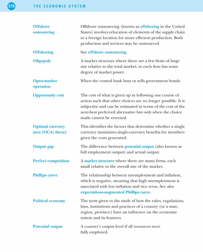
378 T H E E C O N O M I C S Y S T E M
Offshoreoutsourcing
Offshore outsourcing (known as offshoring in the UnitedStates) involves relocation of elements of the supply chainto a foreign location for more efficient production. Bothproduction and services may be outsourced.
Offshoring See offshore outsourcing.
Oligopoly A market structure where there are a few firms of largesize relative to the total market, so each firm has somedegree of market power.
Open-marketoperation
When the central bank buys or sells government bonds.
Opportunity cost The cost of what is given up in following one course ofaction such that other choices are no longer possible. It issubjective and can be estimated in terms of the cost of thenext-best preferred alternative but only when the choicemade cannot be reversed.
Optimal currencyarea (OCA) theory
This identifies the factors that determine whether a singlecurrency maximizes single-currency benefits for membersgiven the costs generated.
Output gap The difference between potential output (also known asfull employment output) and actual output.
Perfect competition A market structure where there are many firms, eachsmall relative to the overall size of the market.
Phillips curve The relationship between unemployment and inflation,which is negative, meaning that high unemployment isassociated with low inflation and vice versa. See alsoexpectations-augmented Phillips curve.
Political economy The term given to the study of how the rules, regulations,laws, institutions and practices of a country (or a state,region, province) have an influence on the economicsystem and its features.
Potential output A country’s output level if all resources werefully employed.

G L O S S A R Y 379
Poverty trap A poverty trap (also sometimes known as anunemployment trap) exists when the opportunity cost ofmoving from unemployment benefits to paidemployment is too high. Unemployed workers are oftenentitled to various benefits in addition to unemploymentpayments. These may include housing or rent allowances,reduced medical costs, food vouchers, etc. On taking uppaid employment, especially of a low-paid nature, thebenefits foregone may be less than the wages earned. Avicious circle of poverty can be created which is difficultto break.
Present value (PV)determination
A method for comparing benefits in different timeperiods in order to compare the future receipt with acurrent receipt of the same value. The standard formulaused to determine present value is
PV = £X(1 + r)T
where PV denotes present value;£X is the amount to be received in the future;r is the market interest rate;T is the number of years before the investment is repaid.
Price cap See price ceiling.
Price ceiling A price that puts an upper limit on the price thatsuppliers can charge.
Price elasticity ofdemand (PED)
The responsiveness of quantity demanded to a change inprice. It is calculated as:
PED = %�Qd/%�P
PED differs at different points on the demand curve. Inabsolute terms (ignoring the minus sign) PED is greaterthan one when the percentage change in quantitydemanded is greater than the percentage change inprice. This is elastic PED. PED is less than one when thepercentage change in quantity demanded is less than thepercentage change in price. This is inelastic PED.

380 T H E E C O N O M I C S Y S T E M
Price elasticity ofsupply (PES)
The responsiveness of quantity supplied to changes inprice. It may be elastic, inelastic or unit elastic.It is computed as the proportional change in quantitysupplied divided by the proportional change inprice:
%�QS/%�P
Price floor A price that suppliers can be sure to receive fortheir output.
Price leadership Where either a dominant firm in the industry sets priceand all others follow or a well-established firm becomesthe ‘leader’ and is trusted with setting the price that allfirms will charge.
Price-cost margin See profit margin.
Prisoner’s Dilemma Exists when the equilibrium from a game generates asub-optimal outcome for all parties involved. Withcommitment (or a binding contract) between the firms,higher pay-offs could be achieved to the benefit of allplayers.
Privatization The sale of government-owned businesses (and associatedassets) in whole or in part to the private sector. Examplesinclude electricity, gas and telecommunicationsindustries.
Producer surplus The benefit to producers due to the difference betweenthe price suppliers are willing to receive for their outputand what they actually receive.
Productdifferentiation
The features or attributes that explain consumers’decisions to buy one variety or brand instead of anotherare the basis for product differentiation.
Productionfunction
A relationship describing how economic activity,specifically output, depends on the factors of production

G L O S S A R Y 381
and technology. It describes a technically efficient use ofthe factors of production and technology necessary toproduce output, i.e. no resources are unemployed.
Profit margin The mark-up over costs that a firm makes or wishes tomake. Some firms will be happy to earn low mark-ups,other firms wish to earn high mark-ups. Also called theprice-cost margin.
Progressive incometax system
A tax system in which individuals pay a higher percentageof their income in tax, the more they earn.
Public goods Goods that would not be provided in a free-marketsystem. They are goods that
• if consumed by one person can still be consumed byothers; non-rival in consumption. Private goods onceconsumed are not available to others.
• if provided, cannot be excluded from the consumptionof anyone who desires the good, even if they do notwish to pay for it. Public goods are non-excludable inconsumption.
Purchasing powerparity (PPP)
A measure of the relative purchasing power of differentcurrencies. PPP is the exchange rate that equates theprice of a basket of identical traded goods and services intwo countries. It is often very different from the marketexchange rate.
Quantity equation M × V = P × Y
where M denotes the nominal money supply in aneconomy, V denotes velocity of money, P denotes theaverage price level, Y denotes the level of real economicactivity and hence P × Y is the nominal value ofeconomic activity (i.e. income or output).
Quotas Quantitative restrictions set by governments on theamount of imports permitted from another customs area.Because quotas limit the supply of a good, they drive theprice of the good up.

382 T H E E C O N O M I C S Y S T E M
Real business cycle(RBC) theory
This theory is based on the view that changes intechnology explain business cycles.
Real interest rate(r)
This is computed as the difference between the nominalinterest rate and the rate of inflation.
r = i − π
where i denotes the nominal rate and π is the rate ofinflation.
Realignments Simultaneous and coordinated devaluation or revaluationof currencies.
Recessionary gap In a recession, the difference between the level ofpotential output and the lower actual output.
Regulatory capture Where regulations set up to protect consumers – to leadto greater competition and lower prices – becomecaptured by the industry for the benefit of producers inthat industry. This happens where producers canconvince the regulator to introduce rulesfavouring producers.
Required reserveratio
The percentage of all deposits received by banks thatmust be held in the bank and not used for loans orother purposes.
Reservation wage The lowest wage a worker will accept to take a job.
Search goods Goods where their quality attributes can be assessedbefore purchase. See also experience goods.
Services Non-material or intangible items of consumption that areconsumed as they are created.
Shoe-leather costs The effect of people holding less currency during periodsof inflation, thereby needing to make more trips to thebank to withdraw cash.
Short run The period of time it takes for a firm to change its scale ofproduction and this depends on its fixed factor ofproduction – usually capital.

G L O S S A R Y 383
Speculativedemand for money
See demand for idle balances.
Spot or cashmarkets
Markets where money changes hands today for goods orservices received today.
Standardizedproducts
Products for which many substitutes are available andwhich use readily available technology in theirproduction. See also differentiated products.
Standardizedunemployment rate
The standardized unemployment rate measures thoseunemployed as people of working age without work whoare available to start work within two weeks and who areactively seeking employment.
Steady state The term used by Solow to describe the equilibrium stateof output and capital stock in the long run. (The term isalso used in physics.) An economy that reaches asteady-state level of capital stock and level of output hasno tendency to change from these levels, ceteris paribus.
Structuralunemployment
Unemployment arising from a permanent decline inemployment in industries located in a particular regionor area.
Subsidy A payment or a tax concession from the government thatreduces producers’ average production costs.
Substitution effect The adjustment in quantity demanded due to the changein relative prices alone, i.e as the price of one goodincreases, people buy less of it preferring its relativelycheaper substitutes.
Supernormal profit See normal profit.
Supply The activities of firms that organize the factors ofproduction to produce output and make it availableto buyers.
Supply chain The resources and processes that are involved inacquiring components and raw materials and includesdelivery of end products to final consumers. It includes

384 T H E E C O N O M I C S Y S T E M
the activities of sellers, distributors, manufacturers,wholesalers and any other service providers andcontributors to the buyer’s decision to buy.
Tacit knowledge Knowledge that is highly personal, not easily visible orexpressible and cannot easily be copied. It usuallyrequires joint, shared activities in order to transmit it.Examples of tacit knowledge include subjective insights,intuitions and hunches.
Tariffs See import tariffs.
Tax wedge The difference between the real wage paid by anemployee and the real wage received by an employee.Differences are accounted for by payroll taxes (usuallyrelated to social insurance/security contributions),income taxes, consumer price taxes.
Total costs (TC) The sum of variable costs and fixed costs incurred by afirm.
Total factorproductivity (TFP)
A measure of the efficiency with which inputs areemployed to produce output. TFP is a catch-all term thatmeasures the effect on output not only of any changes intechnology, but also in the social and political systemsthat affect the quantity and quality of output that aneconomy can produce from its labour and capitalresources. TFP is effectively that portion of output changethat cannot be accounted for by changes in the quantityand quality of labour and capital.
Total revenue (TR) Price times the quantity of goods sold: TR = P × Q .
Total utility (TU) The total benefit perceived by the consumer fromconsumption of a good/service.
Trade barriers Policies or practices that reduce the amount of importsinto a country. Examples include import tariffs andquotas.
Transactions costs The complete price plus non-price costs of a transaction,including search, information, bargaining andpolicing costs.

G L O S S A R Y 385
Unanticipatedinflation
Inflation that takes people by surprise and therefore hasnot been taken into account in economicdecision-making. See also anticipated inflation.
Unemploymenttrap
See poverty trap.
Variable costs (VC) Costs that depend directly on the amount of output afirm produces, such as the costs for production inputsand workers. The higher the quantity produced thehigher the variable costs. See also fixed costs.
Vertical equity Treating people with intrinsically different characteristics(education, experience, abilities) differently in order toreduce the income disparity resulting from theirdifferences. See also horizontal equity.

I N D E X
absolute advantage 37–8, 135AC see average costsACEA see European Automobile
Manufacturers Associationacquisition 234active labour market policies 315advantages of single European currency
277advertising 215, 226Aer Lingus 235AFC see average fixed costsaggregate consumer behaviour 103–7aggregate demand 172–5aggregate economic activity 170–71aggregate expenditure 172–3aggregate supply 171, 175–7, 269Airbus 205–6, 233alliance of economic perspectives 27–9allocation of resources 187ALPS see active labour market policiesalternative targets for monetary policy
270–72fixed and floating exchange rates
270–72Taylor rules and economic judgement
272analysis of unemployment 291–3
classical approach 291–2Keynesian approach 292–3
analytical tools 138anti-competitive practices 17, 226, 315anti-pollution systems 52anticipated inflation 304–5antitrust 231applications of elasticity analysis 98–9appreciation 255, 258arbitrage 259–60, 277arc price elasticity 96artificial scarcity 17Asian Tiger 330, 337
assembled knowledge 58–9assumption of rationality in economics
83–4ATC see average total costattribute combination 102attribute model 101–3Austrian perspectives on competition
221–3Austrian School of Economics 200, 204automatic stabilizers 188autonomous consumption 104, 178–9autonomous investment 143average costs 125–31
explaining U-shaped cost curves 126–31and profit maximization 133
average fixed costs 123–4average output 120–23average product of labour 121average relationships 122–3average total cost 125
BA see British Airwaysbackward bending 71balance of payments 275, 305Bank of England 266Bank for International Settlements 259banking system 244bankruptcy 202, 235, 264banning smoking 109bargaining power 309, 313barriers to entry 135, 199, 315basket of goods 172benchmark 209benefits of competition 232benefits of international trade 184–6benefits of monopoly 213best practice 314, 325beyond demand 77–112
aggregate consumer behaviour 103–7

388 T H E E C O N O M I C S Y S T E M
beyond demand (continued)consumer choice and product attributes
101–3consumer satisfaction – utility 81–4consumers’ response to price changes
93–100demand, consumers and consumer
surplus 90–92demand and the importance of
consumers 78–81government policies – consumer focus
107–9introduction 77–8marginal utility, prices and law of
demand 84–90see also consumers; demand
beyond supply 113–54firms in economic action 114–15firms’ investment behaviour 142–4government influence on supply and
production 144–50introduction 113–14maximizing profits in the long run
131–8organizing economic system around firms
115–31producers’ response to price changes
140–42supply, producers and producer supply
139see also firms; supply
bid down price 212Big Mac Index 4black market 152BMW 49Boeing 205–6, 233bond rankings 265bonds 263–8, 304
inflation and interest rates 266–8boom 160, 273, 298, 306borrowing 105–6bounded rationality 84brand loyalty 212, 214–15breakfast cereals 101–3
bringing AD and AS together177–8
British Airways 235broadband 348–9budget deficit 189, 276budget line 87, 89business cycle 158–65
explanations/causes of business cycles161–4
implications for business andgovernment 165
and real output 158–65business uncertainty 305buyers’ income 43–4
Cambridge School of Economics 14capital 23, 303, 334–5, 344–5capital deepening 342capital goods 23–4capital intensity 191capital requirement 212capital resources 27capital stock investment 335–6capital widening 342cartel 216, 301cash market 261caste system 5Caterpillar tractors 185causes of business cycles 161–4causes of change in exchange rates
258–60causes of differences in natural
unemployment rate 312–14Celtic Tiger 330central bank independence 255, 268central banks 162, 242–5
money multiplier 244–5central planning 61centralized decision-making 20–22ceteris paribus assumption 8–9, 13, 42–4,
160, 331CFC gases 147challenges for car producers 130

I N D E X 389
challenges for the economic system283–320
cross-country differences 314–17inflation 296–305introduction 283–4linking unemployment and inflation
306–314unemployment 284–96
Chamberlin, Edward 213change 223changes in equilibrium 55changes in influences on demand 45–6changes in labour input 341–3changes in technology 343–4chlorofluorocarbons 147Chrysler 130circular flow 156–8classical approach to unemployment
analysis 291–2classification of dangerous substances 52Clayton Act 1914 231co-operative equilibrium 221Coca-Cola 90, 234Coke see Coca-Colacollective wage-bargaining 290–91,
315collusion 216–19, 301comfort products 45commodity 182–3Common Agricultural Policy 57comparative advantage 39comparative measures of economic activity
168competition 134, 197–238
alternative models of competition andmarket structure 204–221
Austrian and traditional perspectives: acomparison 221–3
benefits of 232in the economic system 198–204government regulation of competition
226–35introduction 197–8when markets fail 223–6
competition policy 230–35implementation of 232–5principles 231–2
competition spectrum 229competitiveness 28, 276complements 42–3, 51components of real output 165–70
other measures of economic activity167–8
computation of multiplier 179concentration ratio 205conclusions from the Solow model 345–7congestion charge 43consideration of the euro 274–8constant returns to scale 129constraints 116consumer choice 101–3consumer confidence 17, 44–5consumer focus 107–9consumer preferences 90consumer price index 299–300consumer response to price changes
93–100applications of elasticity analysis 98–9other elasticity examples 99–100price elasticity of demand 94–8
consumer satisfaction 81–4assumption of rationality in economics
83–4consumer surplus 90–92, 289consumer theory 15consumer welfare 92consumers 77–112
aggregate consumer behaviour 103–7choice and product attributes 101–3consumer surplus and consumer welfare
92demand and consumer surplus 90–92demand and importance of 78–81as focus of government policies 107–9marginal utility 84–90response to price changes 93–100and utility 81–4
consumption function 104, 107, 108

390 T H E E C O N O M I C S Y S T E M
consumption goods 77, 79–81consumption smoothing 261–2containerization 183contestable market 202contracting out 49convergence 337, 354, 355convertible bond 264copyright 153cost disadvantage 212cost-push inflation 296–7, 308costs of firm 123–5costs of inflation 304–5costs of international trade 184–6costs of unemployment 285–96countercyclical fiscal policy 188CPI see consumer price indexCR see concentration ratiocreative destruction 164, 236credit cards 240–42cross-country differences:
unemployment and inflation 314–17employment legislation 316–17
cross-price elasticity 100currency stability 273, 276cyclical unemployment 287cyclically adjusted budget 189
Daimler 130deadweight loss 211, 225dealing with AS and AD shocks 187debt 303debt financing 264decentralized decision-making 61–2decision-making 16–22, 61–2, 70–71,
116–17, 253–5decisions of firms 116–17decline in trade barriers 182deflation 171, 299demand 35–76, 78–81, 90–92
consumers and consumer surplus90–92
in the foreign exchange market 256and importance of consumers 78–81
non-price determinants of demand42–6
see also beyond demand; law of demanddemand for balances 246–7demand for bonds 265demand for credit 304demand curve 40–41, 46demand for money 246–7demand schedule 41, 46demand shock 188demand-deficient unemployment 292demand-pull inflation 296–7demography 339dependency ratio 327–31depreciation 142–3, 169, 255, 271, 335–6depression 80description of economic relationships
9–14determinants of demand
non-price 42–6determination of exchange rate 257–8devaluation 271, 276development of the economic system
321–60economic growth over time 331–2income distribution 349–56introduction 322living standards and labour productivity
relationships 322–31modelling economic growth: Solow
growth model 333–49differentiated product 199diminishing returns 127, 215, 348direct competition 233direct taxes 169dis-saving 105–6discouraged workers 284discovery 201–4diseconomies of scale 127, 130disequilibrium 72, 311disposable income 43, 44distortion 146dominant strategy 217–18domino effect 178

I N D E X 391
Dr Pepper 234durable consumption goods 43, 79dynamic efficiency 26–7
easyJet 130, 233ECB see European Central Bankeconomic action 114–15economic activity 155–96
another perspective on 190–92and the circular flow 156–8equilibrium economic activity 170–78equilibrium economic activity and the
multiplier 178–81government activity 187–92international integration 181–7real output and the business cycle
158–65real output and its components 165–70see also macroeconomy
economic analysis 7, 138economic approach 6–9economic efficiency 3economic fundamentals 260–61economic growth 3, 330economic growth over time 331–2economic judgement 272economic and monetary union 275economic perspectives 27–9economic profit 46–8
see also normal profiteconomic relationships 9–14economic resources and markets 2–6economic shock 161, 270, 273, 316economic system 1–34
alliance of economic perspectives 27–9competition in 197–238describing and interpreting economic
relationships 9–14economic resources and markets 2–6economics approach: theory-based
analysis 6–9introducing the economic system 1–2microeconomics and macroeconomics
14–18
positive/normative economics 29–30resource scarcity and prices in the
economic system 18–22resource use, opportunity costs and
efficiency 22–7economic theory 7economies of scale 127, 210–213economies of scope 215economy as a production function 190–92effects of inflation on income distribution
305effects on production of environmental
taxes 147–8efficiency 2–3, 22–7, 133–6, 198efficiency wage 290efficient production 24elastic PED 96–7elasticity see price elasticity of demandelasticity analysis 98–9elderly dependency ratios 329employment legislation 316–17EMU see economic and monetary unionEnd of Life Vehicles EU directive 50, 52,
74endogenous growth 347–9Enron 17entrepreneurship 23, 201–4, 350environmental taxes 147–8equilibrium 55, 63, 71–2
in the labour market 71–2equilibrium economic activity 170–81
aggregate demand 172–5aggregate supply 175–7bringing AD and AS together: the short
run 177–8and the multiplier 178–81price level 171–2
equilibrium price 53–5, 91equity financing 264ERM see exchange rate mechanismeuro 255–9, 274–8
how it scores under the four OCA factors277–8

392 T H E E C O N O M I C S Y S T E M
European Automobile ManufacturersAssociation 74
European car industry 111–12European Central Bank 179, 242, 250–51,
258, 271, 277European Monetary Union 189evidence on convergence 354ex-ante real interest rate 253–4ex-post real interest rate 253–4exchange 36–40, 240–41
and money 240–41exchange rate 255–60, 270–72
causes of changes in 258–60determination 257–8
exchange rate mechanism 275expansionary fiscal policy 188expectations of inflation 253–5expectations-augmented Phillips curve
306–7expectations-generated inflation 308expected future prices 44, 51expenditure approach 165expenditure categories 156experience curve effect 212experience goods 225explaining U-shaped cost curves 126–31explanation of business cycles 161–4explanation of growth 344–5explanation of international productivity
differences 346explanation of international trade growth
182–4extent of competition in the economy
198–204competition as a process 199–201entrepreneurship, discovery and market
process 201–4externalities 147, 224
factor earnings 169factors of production 2, 48–50fallacy of composition 106, 186Federal Reserve 242, 250, 258, 272female participation in the workforce 316
fertility rate 329fiat money 241final goods 168Finance Act 2001 108financial markets 239–82
foreign exchange market 255–60international monetary integration
272–8introduction 239–40liquidity, central banks and money supply
242–5monetary policy 268–72money demand 246–7money and exchange 240–41money market: demand and supply
247–51quantity theory of money and explaining
inflation 251–5speculation in markets 260–68
firm output 120–23see also product
firms 113–54in economic action 114–15government influence on supply and
production 144–50investment behaviour 142–4maximizing profits in the long run
131–8organizing economic system around
115–31producers’ response to price changes
140–42supply, producers and producer surplus
139first-mover advantage 136fiscal drag 305fiscal policy 188, 298Fisher equation 254fixed costs 123–4fixed exchange rates 270–72fixed factors of production 116floating exchange rates 270–72floor prices 141food labelling 52, 226

I N D E X 393
foreign bond 264foreign exchange market 158, 255–60
causes of changes in exchange rates258–60
demand in 256exchange rate determination 257–8supply in 256–7
fractional reserve system 244Franklin, Benjamin 164free entry 202free-market outcome 35free-market system 61–2, 204, 289free-rider problem 22frictional unemployment 286–7, 291, 308Friedman, Milton 306full employment output 272full-time workers 316functions of money 240–41futures market 261
game of chance 222game theory 217–20gas emissions 147GDP deflator 300General Agreement on Tariffs and Trade
186, 354golden rule level of capital 340–41government activity 187–92
economy as a production function190–92
government contribution to inflation303–4
see also inflationgovernment effect on prices 56–8
price ceiling 56–7price floor 57problems of price ceilings and floors
57–8government expenditure 115government influence on supply and
production 144–50government policies 107–9government regulation of competition
226–35
competition policy 230–35competition spectrum 229structure, conduct and performance
229–30government regulations 52,
204Great Depression 80–81, 164Greenspan, Alan 250grey imports 152–3grey market for cars 152–3Groningen Growth and Development
Centre 193gross domestic product 166–70
what it does not measure 169–70gross national income 43, 166gross national product 168–70
what it does not measure 169–70growth accounting 344growth differential 258–9growth of the economic system 3,
321–60
haggling 62hard investment 336Harmonized Index of Consumer Prices
193Hayek, Friedrich August von 60–61, 75,
200, 223, 230hazardous waste 74HDI see human development indexhealth and safety standards 226Herfindahl Index 205Hitler, Adolf 81horizontal equity 351household saving rates 338–40how euro scores under the four OCA
factors 277–8human capital 24, 296, 348human development index 324
Iberia Airlines 235IBM 222idiosyncratic knowledge 59idle balances 246–7

394 T H E E C O N O M I C S Y S T E M
illegal accounting methods 17ILO see International Labour Organizationimperfect competition 205implementation of competition policy
232–5implications of business cycles 165implications of change in influence on
demand 45–6implications of market failure 225–6implicit collusion 216–17importance of consumers 78–81
consumption goods 79–81incentive 21, 39, 51, 142, 355income 168–70income distribution 105, 305, 321–60
intra-country 351–6welfare perspective 349–51
income effect 42, 87–90income elasticity of demand 99–100income injection 158, 298income method of measuring economic
activity 167–8increased quality of labour 27increased quantity of labour 26increasing opportunity costs of
production 25independence of central banks
255, 268index numbers 10indifference curve 87–8indirect competition 233indirect taxes 169individual supply decision 70–71indivisibilities in production 128industry labour demand curve 64inelastic PED 96inelastic PES 140inferior good 89, 99inflation 171, 251–5, 266–72, 276,
283–320bonds and interest rates 266–8costs of anticipated and unanticipated
inflation 304–5
cross-country differences:unemployment and 314–17
governments’ contribution to inflation303–4
inflation expectations, interest rates anddecision-making 253–5
inflationary gap 297–9linking unemployment and 306–314measurement of 296–7trends in international price levels
299–303see also challenges for the economic
systeminflation differential 258–9inflation expectations 253–5, 304inflationary gap 297–9influences on demand 45–6influences on supply and production
144–50environmental taxes 147–8international trade 145–7tax incidence 149–50using subsidies 145–7
information 58–62decentralized decision-making 61–2
information asymmetries 223–6innovation 21, 163, 198–200innovation incentives 21input see labour inputinsider–outsider model 303intellectual property 153intention 40interest rate differential 258interest rate effect 174–5interest rates 248–51, 253–5, 266–8,
276, 304bonds and inflation 266–8and decision-making 253–5
intermediate goods 168international business cycle 159
see also business cycleinternational competitiveness 305international dependency ratios 328international inflation rates 300

I N D E X 395
international integration 181–7benefits and costs of international trade
184–7explaining growing international trade
182–4see also international trade
International Labour Organization 285international monetary integration 272–8
considering the euro 274–8international price level trends 299–303international trade 145–7, 181–7
benefits and costs 184–7explaining growing international trade
182–4international trade effect 175interpretation of economic relationships
9–14intervention 226intra-country income distribution 351–6
evidence on convergence 354trade and development 354–6
introduction to the economic system 1–2inventory 45, 142–3, 202inventory investment 79investment behaviour of firms 142–4investment in bond markets 263–6investment function 143–4‘invisible hand’ concept 60
see also Smith, AdamIranian Revolution 302Irish Special Savings Investment Accounts
108irrational exuberance 250
Keynes, John Maynard 164, 292Keynesian approach to unemployment
analysis 292–3, 298knowledge 58–62, 201–2, 221–3, 230
see also informationKyoto Protocol 147
labour demand 64–70labour input 325, 341–5labour laws 165
labour market 64–72, 289–90equilibrium in the labour market 71–2labour demand 64–70labour supply 70–71
labour market analysis 286–91labour market flexibility 316labour output see outputlabour productivity 21, 322–31, 333, 347
dependency ratio 327–31see also living standards
labour supply 70–71lack of stability effects 305law of demand 84–90
income and substitution effects 87–90see also beyond demand; demand
law of diminishing returns 66–7leakage 158, 180lean production 144legal protection 213liberalization 228licensing 204linking unemployment and inflation
306–314causes of differences in natural
unemployment rates 312–14model explaining natural unemployment
rate 309–312liquidity 242–7living standards 31, 322–31, 350
definition 3dependency ratio 327–31see also labour productivity
loan term 248–9lobby groups 144, 317logistics 184London ForEx 260long run 116–17long-run aggregate supply 176–7long-run aggregate supply curve 176–7long-run average cost 129long-run average cost curve 131, 208, 214long-run equilibrium 208–9loss of purchasing power 305LRAC see long-run average cost

396 T H E E C O N O M I C S Y S T E M
LRAS see long-run aggregate supplylumpy investment 162
macroeconomic consumption behaviour103–7
macroeconomics 14–18environment for economic decisions
16–18macroeconomy 155–96, 310
economic activity and the circular flow156–8
equilibrium economic activity 170–78equilibrium economic activity and the
multiplier 178–81government activity 187–92international integration 181–7introduction 155–6real output and the business cycle
158–65real output and its components 165–70see also economic activity
maintenance of brand loyalty inmonopolistic competition 215
margin-setting curve 310, 312marginal analysis 117marginal costs 25–6, 69, 125–31
explaining U-shaped cost curves 126–31marginal output 120–23marginal product of capital 344marginal product of labour 65, 121, 345marginal propensity to consume 104–5,
108marginal rate of substitution 88marginal relationships 122–3marginal revenue 118–19
product of labour 67, 69marginal revenue function 118–19marginal utility 82–90
income and substitution effects 87–90mark-up 309market abuse 235market analysis 35–76
demand 40–46equilibrium 63
exchange 36–40government affecting prices 56–8information and knowledge in the
market system 58–62introduction 35–6market interaction 52–5market labour 64–72supply 46–52
market clearing price 52market concentration 204market economy 62market failure 22, 223–6
implications of market failure225–6
why markets fail 223–5market failure implications 225–6market failure types 223–5
externalities 224information asymmetries 224–5monopoly power 224natural monopoly 224public goods 223–4
market interaction 52–5changes in equilibrium 55
market power 204market process 201–4market structure 204–221markets 2–6, 204Marshall, Alfred 13–14maximization of profits in the long run
131–8maximizing profits over the short run
137–8profit maximization, normal profit and
efficiency 133–6maximization of profits in the short run
137–8economic analysis 138
MC see marginal costsmeasures of economic activity
167–70GNP, GDP and income 168–70
menu costs 305MES see minimum efficient scale

I N D E X 397
microeconomics 14–18, 356environment for economic decisions
16–18Microsoft 222millennium development goals (UN)
354minimum efficient scale 129minimum wage 287–91mismatch 314Mitchell, B.R. 299model explaining natural unemployment
rate 309–312modelling economic growth 333–49
conclusions from the Solow model345–7
endogenous growth 347–9explaining growth: labour, capital and
technology 344–5more on savings 337–41Solow model and changes in labour input
341–3Solow model and changes in technology
343–4models of competition and market
structure 204–221monopolistic competition 213–15monopoly 209–211oligopoly 215–21perfect competition 206–9perfect competition vs. monopoly
211–13monetary policy 242, 268–72
alternative targets 270–72difficulties in targeting money supply
269–70Taylor rules and economic judgement
272Monetary Policy Committee 271money 239–82
demand 246–7and exchange 240–41international monetary integration
272–8
liquidity, central banks and money supply242–5
market: demand and supply 247–51monetary policy 268–72quantity theory of money and explaining
inflation 251–5see also financial markets
money demand 246–51money market 247–51
nominal and real interest rates249–51
which interest rate 248–9money multiplier 244–5money supply 242–5, 247–51monopolistic competition 213–15
maintaining and enhancing brand loyalty215
monopoly 209–211benefits 213vs. perfect competition 211–13
monopoly power 224Moody’s 265mortgages 248–9MPC see marginal propensity to consumeMPPL see marginal physical product of
labourMR see marginal revenueMSC see margin-setting curvemultiplier 178–81municipal bond 264
NAIRU see non-accelerating inflation rate ofunemployment
nanny state 109Nash equilibrium 219, 237Nash, John 219National Association of Software and
Service Companies 184national exchange rates 15–16national income 78, 162national output 78, 299National Socialist Workers Party 81national statistics 171natural monopoly 210, 224

398 T H E E C O N O M I C S Y S T E M
natural rate of unemployment 286–7,306–314
causes of differences in 312–14explanatory model 309–312
neoclassical growth model 333see also Solow growth model
net exports 115, 175net investment 143neuromarketing 90new growth model 347NGOs see non-governmental organizationsNissan 130nominal amounts 11nominal inflation 249nominal interest rates 249–51non-accelerating inflation rate of
unemployment 286non-durable goods 79, 81non-governmental organizations 350non-price competition 215non-price determinants of demand 42–6
buyers’ income 43–4complements and substitutes 42–3consumer confidence 44–5expected future prices 44implications of changes in influences on
demand 45–6population 44preferences 44price of related goods/services 42–3
non-unionized workers 303, 309normal good 89, 99normal profit 48, 133–6
see also economic profitnormative economics 29–30
see also positive economicsnumber of suppliers 51
OCA see optimal currency areaOECD see Organization for Economic
Cooperation and Developmentoffshore outsourcing 184–5offshoring see offshore outsourcingoil prices 42, 162, 301–2, 324
and inflation 301–2oligopoly 215–21
and game theory 217–19Prisoner’s Dilemma 219–21
OPEC see Organization of PetroleumExporting Countries
open-market operation 243, 247, 303–4opportunity costs 18, 22–7, 37–9, 47, 86opposition 223optimal currency area 273optimal form of organization 61–2Organization for Economic Cooperation
and Development 3, 32, 216, 301,316, 329, 337
organization of economic system aroundfirms 115–31
firm costs 123–5firm output 120–23firm revenue 117–20firms’ decisions and role of time
116–17marginal and average costs 125–31marginal and average output 120–23product 120–23
Organization of Petroleum ExportingCountries 142
output 120–23, 158–70output gap 160outsourcing 49, 314overproduction 141overspending 303ownership rights 203–4
paradox of thrift 106parallel imports 152–3Parmalat 17part-time workers 316, 343patents 135, 153, 203patterns in real output 159PED see price elasticity of demandPenn World Table 31, 79Pepsi 90, 234perfect competition 204–9, 222
long-run equilibrium 208–9

I N D E X 399
short-run equilibrium 207–8vs. monopoly 211–13
perfect elasticity 141perfect inelasticity 141persistent economic growth 347perspectives on competition compared
221–3PES see price elasticity of supplyPhelps, Edmund 306Phillips curve 306–8Phillips, William 306physical capital 348political economy 5pollution 52, 147, 170population 44, 351positive economics 29–30
see also normative economicspotential output 160, 175–6poverty trap 326PPF see production possibility frontierpreferences 44, 105
see also consumer preferencespresent value 266–8price cap see price ceilingprice ceiling 56–7, 142, 289
problems of 57–8price changes 93–100, 140–42price changes and consumer response
93–100price elasticity of demand 94–8
cross-price elasticity 100income elasticity 99–100other examples 99–100some special cases 98and total revenue 96–8
price elasticity of supply 140, 142price fixing 17price floor 57–8price leadership 216–17price level 171–2price of production factors 48–50price and quantity effects 11, 14price ratios 85–6price of related goods/services 42–3, 51
price sensitivity 93–4, 98–9, 302price-cost margin 309prices 18–22, 84–90
using resources and centralizeddecision-making 20–22
principles of competition policy 231–2Prisoner’s Dilemma 219–21private property rights 61privatization 228pro-competitive practices 315problems of price ceilings and floors 57–8process of competition 199–201process of economic analysis 7producer response to price change
140–42producer surplus 139producers 139product 120–23
see also firm outputproduct attributes 101–3
attribute model 101–3product differentiation 101, 135production function 190–92, 334, 348production possibility frontier 23–7, 348productivity advantage 38profit margin 309profit maximization in the long run 131–8
normal profit and efficiency 133–6profit maximization, normal profit and
efficiency 133–6profit maximization in the short run
137–8economic analysis 138
profitability 290property bubble 250property rights 349psychology 45public debt 276public goods 21–2, 187, 223–6public interest 27public sector employment 108–9purchasing power parity 3–4, 41–2
adjustment 3

400 T H E E C O N O M I C S Y S T E M
quantity theory of money 251–5, 304inflation expectations, interest rates and
decision-making 253–5quasi-fixing 271quota 182, 187
R&D see research and developmentrankings of bonds 265rationality in economics 83–4real amounts 11real business cycle 162
see also business cyclereal business cycle theory 162–3real economic activity 166real interest rates 249–51real output 158–70
and the business cycle 158–65and its components 165–70patterns in 159
real wage-setting curve 310, 313real wealth effect 174realignment 275the real thing 153reasons for inflation 301recession 80, 160, 176, 273, 287recessionary gap 293–5redistribution effect 225redundancy 316registered design rights 153regulation of competition 226–35regulatory capture 227related goods/services price 42–3, 51relative price 86Renault 130required reserve ratio 244research and development 213, 349reservation wage 70reserve ratio 244reskilling 315resource scarcity 18–22
using resources and centralizeddecision-making 20–22
resources 18–22, 187, 297restrictions 199
restructuring 49, 235returns to large-scale production 128revenue of firm 117–20revenue maximization 118risk 249robotics 49, 124robustness 236role of time 116–17Rover 49RWS curve see real wage-setting curveRyanair 130, 233
Sabena 235savings 337–41savings axis 105savings function 106scale economies 136scale of world poverty 354Schumpeter, Joseph 136, 163–4, 200, 203,
213scientific knowledge 58SCP paradigm see structure, conduct,
performance paradigmSEA see Single European Actseasonal unemployment 287self-sufficiency 38Sen, Amartya 354services 79, 81Sherman Act 1890 231shoe-leather costs 305short run 116–17short-run average cost curve 130–31short-run average total costs 137–8short-run equilibrium 207–8short-term fluctuation 156, 170shortage 53Single European Act 274Smith, Adam 3, 20, 60, 128, 184, 203soft investment 336Solow growth model 333–49, 356
and changes in labour input 341–3and changes in technology 343–4conclusions from 345–7endogenous growth 347–9
I N D E X 401
explaining growth: labour, capital andtechnology 344–5
more on savings 337–41Solow residual 345Solow, Robert 333spare capacity 176special cases of price elasticity of
demand 98special savings accounts 108specialization 128, 203spectrum of competition 229speculation 246, 258–68, 277
bonds, inflation and interest rates266–8
investment in bond markets 263–6sports utility vehicle 45–6, 51, 55spot market 261SRAC see short-run average cost curvestabilization policy 187–8Standard & Poor’s 265standardized product 199standardized unemployment rate 285Starbucks 4start-ups 27static efficiency 26steady state 335–7, 347sticky wages 292, 294, 298, 302, 308structural unemployment 286–7, 308structure, conduct, performance paradigm
229–30subsidies 144–7, 234–5, 355subsidizing 145, 349, 355substitutes 41–3, 51, 175, 233substitution effect 41, 87–90summary of market characteristics 220–21sunspot theory 164supernormal profit 48, 133–6, 207–211,
214supplier number 51supply 35–76, 139
expected future prices 51in the foreign exchange market 256–7government regulations 52number of suppliers 51
prices of factors of production 48–50prices of related goods 51producers and producer surplus 139
supply chain 183supply curve 47, 50supply of money 242–5supply schedule 47, 50surplus 53, 90–92, 139SUV see sports utility vehicleswitching costs 315
tacit knowledge 59, 201Tall Latte Index 4targeting monetary supply 269–72
alternative targets 270–72difficulties in 269–70
tariff 182, 184, 187, 355tax incidence 149–50tax rate 108, 303tax wedge 314–15
see also wedgetaxation 187Taylor rules 272technology 27, 343–5TFC see total fixed costsTFP see total factor productivitytheory-based analysis 6–9time 116–17time-series data 12total costs 123–5total factor productivity 345, 347total fixed costs 123–4total output 120total revenue 96–7, 118
and price elasticity of demand 96–8total utility 82–3total variable cost curve 124–5tourism 259, 287trade barriers 182trade deficit 181, 271trade and development 354–6trade restrictions 186, 354trademarks 153

402 T H E E C O N O M I C S Y S T E M
traditional perspectives on competition221–3
transaction costs 62transactions 246transfer payment 157, 187transport deregulation 183Treaty of Maastricht 274–5Treaty of Rome 229, 232, 274trend line 14trends in international price levels
299–303TVC see total variable cost curvetypes of market failure 223–5types of unemployment 286–91
unanticipated inflation 304–5unemployment 283–320
analysing unemployment 291–3causes of differences in natural rates of
312–14costs of 295–6cross-country differences: inflation and
314–17labour market analysis 286–91linking inflation and 306–314model explaining natural rate of
309–312rate 284–6and the recessionary gap 293–5types of unemployment 286–91see also challenges for the economic
systemunemployment benefits 292unemployment trap 326United Nations 354unpredictability 222–3
unregistered design rights 153use of resources 20–27
opportunity costs and efficiency 22–7use of subsidy 145–7utility 81–4
value-added method of measuringeconomic activity 167–8
variable costs 123velocity 251–2vertical equity 351Virgin Airlines 235
wage rise negotiations 303–4, 313wage-bargaining 290–91, 302, 304, 315Wall Street Crash 80waste 50, 74wealth 105Wealth of Nations 3wedge 147, 166, 314–15welfare economics 92, 160, 326, 356what GNP and GDP do not measure
169–70women 316world poverty 354World Trade Organization 16, 146, 186,
354World War Two 81, 301, 324WorldCom 17WTO see World Trade Organization
Yom Kippur War 302young dependency ratios 329
zero-coupon bond 264zero-sum game 200