Chapter 1 - Murdoch Research Repository - Murdoch University

THERMODYNAMIC AND RELATED STUDIES OF
AQUEOUS COPPER(II) SULFATE SOLUTIONS
Chandrika Akilan B.Sc.Hons (Murdoch University)
This thesis is presented for the degree of Doctor of Philosophy of Murdoch University
Western Australia
2008

I declare that this thesis is my own account of my research and contains as its main content work which has not previously been submitted for a degree
at any tertiary education institution.
Chandrika Akilan
Abstract
This thesis describes a systematic investigation of the thermodynamic quantities
associated with the interaction between Cu2+ and SO42– in aqueous solution. A variety of
techniques including UV-Visible spectrophotometry, Cu(II) ion-selective electrode
potentiometry, dielectric relaxation spectroscopy and titration calorimetry have been
used.
The values for the (aq) association constants determined by UV-Vis
spectrophotometry in NaClO4 media as a function of ionic strength were in good
agreement with published data but were lower than the values obtained from Cu(II) ion -
selective electrode potentiometry. The source of this difference was traced to the
presence of solvent-separated ion pairs which are only partially detected by UV-Vis
spectrophotometry. This was shown by a detailed investigation of CuSO4(aq) over a
wide range of concentrations using modern broad-band dielectric relaxation spectroscopy
(DRS). This technique revealed the presence of three ion-pair types: double solvent-
separated, solvent-shared and contact ion pairs.
04CuSO
Calorimetric titrations using the log KA values determined by potentiometry, have
provided for the first time reliable values for the enthalpy and entropy changes associated
with complex formation between Cu2+(aq) and SO42–(aq) system over range of ionic
strengths (in NaClO4 media). These data were fitted to a specific ion interaction model to
obtain the standard state value which was in excellent agreement with the values obtained
in other studies and from the DRS work in this study.
In addition, investigations have been carried out into the physicochemical properties,
(osmotic coefficients, densities, heat capacities, solubilities and viscosities) of ternary
mixtures of CuSO4(aq) with Na2SO4(aq) or MgSO4(aq). The isopiestic measurements
(water activities) of the mixtures were in general well described by Zdanovskii’s rule,
especially for the mixtures of CuSO4 with MgSO4. The densities of the ternary mixtures
of CuSO4 with MgSO4 were found to follow Young’s rule of mixing but those of CuSO4
with Na2SO4 deviated from linearity. The solubilities of the salts in their ternary
mixtures agree well with literature data and show that the solubility of MgSO4 or CuSO4
decreases with increasing Na2SO4 concentration. The viscosities of all the ternary
mixtures show clear negative departures from 'Young’s rule' type behaviour.
Publications
The following publications have arisen from work completed by the candidate for the
present thesis.
Chandrika Akilan, Nashiour Rohman, Glenn Hefter and Richard Buchner, Ion
association and Hydration in Aqueous Solutions of Copper (II) Sulfate from 5 to 65oC by
Dielectric Spectroscopy, J. Phys. Chem. B, 110 (30), 14961 -14970, (2006).
Chandrika Akilan, Glenn Hefter, Peter May and Simon Schrödle, Thermodynamics of
Cu2+/SO42– Association in Aqueous Solution, 12th International Symposium on Solubility
Phenomena and Related Equilibrium Processes, Freiberg, Germany, July 24-29, Book of
Abstracts, p 23, (2006).
Chandrika Akilan, Lan-Chi Königsberger, Glenn Hefter and Peter May, Physicochemical
properties of mixed sulfate electrolyte systems, 30th International Conference on Solution
Chemistry, Murdoch University, Perth, Australia, July 16-20, Book of Abstracts, p 81,
(2007).
Chandrika Akilan, Lan-Chi Königsberger, Glenn Hefter and Peter May, Physicochemical
properties of mixed sulfate electrolyte systems, The Royal Society of Western Australia
Promoting Science, Postgraduate Symposium 2007, University of Western Australia,
Perth, Australia, September 11 (2007).

Acknowledgements
I would like to thank sincerely my supervisors, Associate Professor Glenn Hefter and Professor Peter M. May for their continuous guidance, advice, encouragement and help throughout this entire project. I would like to express my gratitude to Apl. Professor Richard Buchner, Institut fuer Physikalische und Theoretische Chemie, Universitaet Regensburg, Germany for his role in modeling and interpreting my dielectric relaxation spectra and Dr Nashiour Rohman for his support. I would also like to express my gratitude to Dr Simon Schrödle for his help and support during the titration calorimetry studies and data analysis. I would extend my sincere thanks to Dr. W.W. Ruldolph for making available some of his unpublished Raman data. My thanks also go to Dr Paul Brown, Rio Tinto, for fitting my enthalpy of formation data to SIT model. I would like sincerely to thank Dr Eric Königsberger and Dr. Lan-Chi Königsberger for their help and advice throughout this project. Thanks are also extended to Dr Nimal Perera for his tremendous support during the time of my UV-Vis spectrophotometric titrations and data analysis. I am further indebted to the following individuals for their help in various aspects: Mr. Ernie Etherinton, Mr. Kleber Claux and Mr. John Snowball of the Murdoch University Mechanical and Electronic workshops. Mr. Doug Clarke, Mr. Tom Osborne and Mr. Andrew Forman of the Chemistry Department technical staff. The support and friendship of my fellow research students, friends and family have been deeply appreciated and are gratefully acknowledged. Finally, I would like to thank the Australian Government, Alcan Engineering Pty. Ltd., Alcoa World Alumina Australia, Comalco Aluminium Limited and Worsley Alumina Pty. Ltd for their financial assistance in the form of an Australian Postgraduate Award (Industry) scholarship and also to Parker Cooperative Research Centre for integrated Hydrometallurgy Solutions for their financial assistance.

Contents
Abstract
Publications
Acknowledgements
Contents
List of tables
List of figures
Abbreviations and symbols
Chapter One: Introduction
1.1. THE IMPORTANCE OF CuSO4 SOLUTIONS
1.2 COPPER MINERALS 1.2.1 Occurrence
1.2.2 Pyrometallurgical extraction
1.2.3 Hydrometallurgical extraction
1.3 COPPER(II) SULFATE SOLUTIONS
1.4 THEORIES OF IONIC SOLUTIONS
1.5 ION PAIRING
1.5.1 Formation of ion pairs
1.5.2 The Eigen-Tamm Mechanism
1.6 ION ASSOCIATION STUDIES ON AQUEOUS Cu2+/SO42–
1.6.1 Association constants
1.6.2 Enthalpy and entropy values
1.7 PROPERTIES OF CuSO4 IN MIXED-ELECTROLYTE
SYSTEMS
1.8 OVERVIEW OF THIS RESEARCH
Chapter Two: UV-Visible spectrophotometry
2.1 THEORY
2.2 SOLUTION PREPARATION
2.2.1 Reagents
2.2.2 Difficulties and precautions during solution
preparation
2.3 INSTRUMENTATION AND PROCEDURE 2.3.1 Titration cell
2.3.2 Titration procedures
2.3.3 Titration method
2.4 DATA ANALYSIS
2.5 THE SPECFIT PROGRAM
2.6 RESULTS AND DISCUSSION 2.6.1 Association constants by UV-Vis
Spectrophotometry
2.6.2 Comparison with literature data
2.6.3 Standard state association constant
2.6.4 Possible occurrence of a second complex
Chapter Three: Potentiometry
3.1 INTRODUCTION
3.2 EXPERIMENTAL STRATEGY
3.3 EXPERIMENTAL 3.3.1 Reagents and glassware
3.3.2 Electrodes
3.3.3 Titration apparatus
3.3.4 Titration procedure
3.4 DATA ANALYSIS
3.5 CHARACTERISATION OF THE BEHAVIOUR OF THE
Cu2+-ISE
3.6 FORMATION CONSTANT OF BY Cu2+-ISE 04CuSO
POTENTIOMETRY
3.7 COMPARISON OF PRESENT RESULTS WITH UV-Vis
RESULTS
3.8 LITERATURE COMPARISON
3.9 STANDARD STATE ASSOCIATION CONSTANT
3.10 HIGHER-ORDER COMPLEXES
Chapter Four: Dielectric Relaxation
Spectroscopy
4.1 DIELECTRIC THEORY
4.2 DRS OF CuSO4(aq) SOLUTIONS
4.3 EXPERIMENTAL 4.3.1 Instrumentation
4.3.2 Solution preparation
4.3.3 Calibration of the VNA
4.4 MEASUREMENT PROCEDURE AND DATA ANALYSIS
4.5 RESULTS AND DISCUSSION 4.5.1 General features of ion association
4.5.2 Analysis of the ion association
4.5.3 Ion-pair relaxation times
4.5.4 Solvent relaxation and ion hydration
4.6 IMPLICATIONS OF THE PRESENT WORK
Chapter Five: Calorimetry of the Cu2+/SO42–
interaction
5.1 APPLICATION OF TITRATION CALORIMETRY TO
M2+/SO42– ASSOCIATION
5.2 EXPERIMENTAL 5.2.1 Apparatus
5.2.2 Electrical calibration
5.2.3 Chemical testing
5.2.4 Materials
5.2.5 Titration protocol
5.2.6 Titration procedure
5.2.7 Heats of dilution (Qd)
5.2.8 Heats of reaction (Qr)
5.3 RESULTS AND DISCUSSION 5.3.1 Heats of dilution results
5.3.2 Heats of reaction results
5.3.3 Enthalpy and entropy changes
5.3.4 Standard enthalpy change (ΔHo) for 04CuSO (aq) formation
5.3.5 Comparison with literature data
5.3.6 Comparison with other M2+/SO42– systems
5.4 CONCLUDING REMARKS
Chapter Six: Physicochemical properties of
binary and ternary solutions of copper and related
sulfates
6.1 BACKGROUND 6.1.1 Importance of physicochemical properties
6.1.2 Selection of systems
6.2 TECHNIQUES 6.2.1 Isopiestic method
6.2.2 Density
Apparent molar volumes
6.2.3 Heat capacity
6.2.4 Solubility
6.2.5 Viscosity measurements
6.3 EXPERIMENTAL 6.3.1 Isopiestic measurements
6.3.2 Density measurements
6.3.3 Heat capacity measurements

6.3.4 Solubility measurements
6.3.5 Viscosity measurements
6.4 ISOPIESTIC MOLALITIES AND OSMOTIC
COEFFICIENTS RESULTS
6.5 DENSITY RESULTS
6.6 HEAT CAPACITY RESULTS Calorimeter asymmetry
6.7 SOLUBILITY RESULTS
6.8 VISCOSITY RESULTS
6.9 CONCLUDING REMARKS
Chapter Seven: Conclusion and future work
Future work
Appendix
References
List of tables
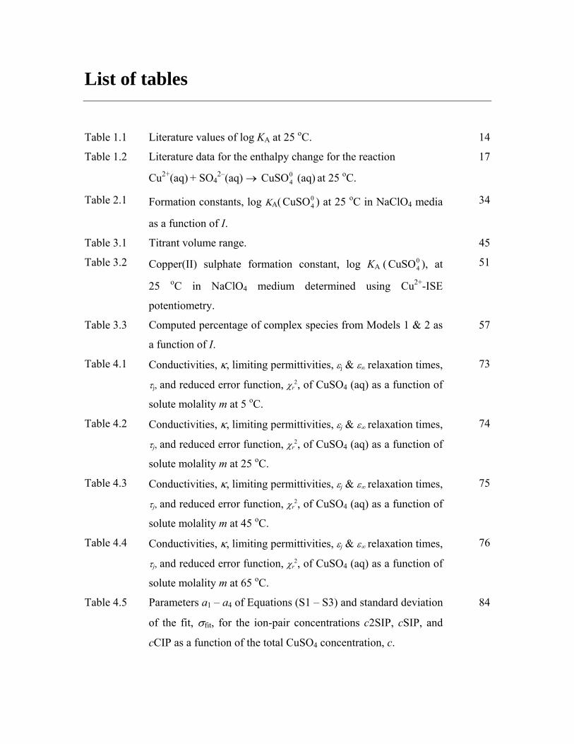
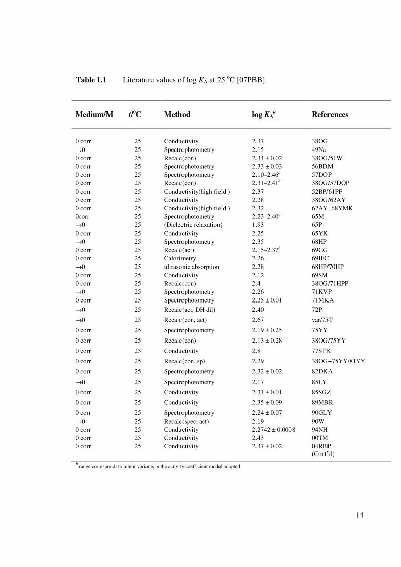
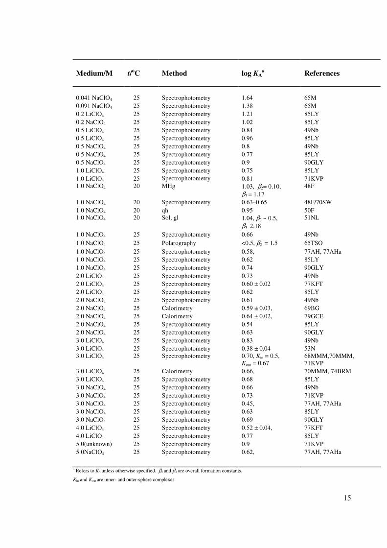
Table 1.1 Literature values of log KA at 25 oC. 14
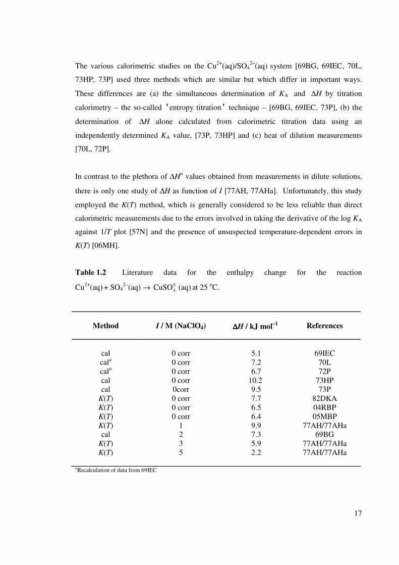
Table 1.2 Literature data for the enthalpy change for the reaction
Cu2+(aq) + SO42–(aq) → (aq) at 25 oC. 0
4CuSO
17
Table 2.1 Formation constants, log ΚA( ) at 25 oC in NaClO4 media
as a function of I.
04CuSO 34
Table 3.1 Titrant volume range. 45
Table 3.2 Copper(II) sulphate formation constant, log KA ( ), at
25 oC in NaClO4 medium determined using Cu2+-ISE
potentiometry.
04CuSO 51
Table 3.3 Computed percentage of complex species from Models 1 & 2 as
a function of I.
57
Table 4.1 Conductivities, κ, limiting permittivities, εj & ε∞ relaxation times,
τj, and reduced error function, χr2, of CuSO4 (aq) as a function of
solute molality m at 5 oC.
73
Table 4.2 Conductivities, κ, limiting permittivities, εj & ε∞ relaxation times,
τj, and reduced error function, χr2, of CuSO4 (aq) as a function of
solute molality m at 25 oC.
74
Table 4.3 Conductivities, κ, limiting permittivities, εj & ε∞ relaxation times,
τj, and reduced error function, χr2, of CuSO4 (aq) as a function of
solute molality m at 45 oC.
75
Table 4.4 Conductivities, κ, limiting permittivities, εj & ε∞ relaxation times,
τj, and reduced error function, χr2, of CuSO4 (aq) as a function of
solute molality m at 65 oC.
76
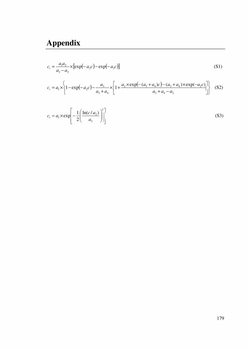
Table 4.5 Parameters a1 – a4 of Equations (S1 – S3) and standard deviation
of the fit, σfit, for the ion-pair concentrations c2SIP, cSIP, and
cCIP as a function of the total CuSO4 concentration, c.
84
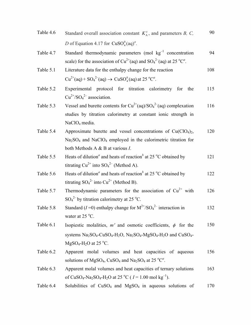
Table 4.6 Standard overall association constant , and parameters B, C,
D of Equation 4.17 for (aq)a.
oKA
04CuSO
90
Table 4.7 Standard thermodynamic parameters (mol kg–1 concentration
scale) for the association of Cu2+(aq) and SO42–(aq) at 25 oCa.
94
Table 5.1 Literature data for the enthalpy change for the reaction
Cu2+(aq) + SO42–(aq) → (aq) at 25 oCa. 0
4CuSO
108
Table 5.2 Experimental protocol for titration calorimetry for the
Cu2+/SO42– association.
115
Table 5.3 Vessel and burette contents for Cu2+(aq)/SO42–(aq) complexation
studies by titration calorimetry at constant ionic strength in
NaClO4 media.
116
Table 5.4 Approximate burette and vessel concentrations of Cu(ClO4)2,
Na2SO4 and NaClO4 employed in the calorimetric titration for
both Methods A & B at various I.
120
Table 5.5 Heats of dilutiona and heats of reactionb at 25 oC obtained by
titrating Cu2+ into SO42– (Method A).
121
Table 5.6 Heats of dilutiona and heats of reactionb at 25 oC obtained by
titrating SO42- into Cu2+ (Method B).
122
Table 5.7 Thermodynamic parameters for the association of Cu2+ with
SO42– by titration calorimetry at 25 oC.
126
Table 5.8 Standard (I =0) enthalpy change for M2+/SO42– interaction in
water at 25 oC.
132
Table 6.1 Isopiestic molalities, m′ and osmotic coefficients, φ for the
systems Na2SO4-CuSO4-H2O, Na2SO4-MgSO4-H2O and CuSO4-
MgSO4-H2O at 25 oC.
150
Table 6.2 Apparent molal volumes and heat capacities of aqueous
solutions of MgSO4, CuSO4 and Na2SO4 at 25 oCa.
156
Table 6.3 Apparent molal volumes and heat capacities of ternary solutions
of CuSO4-Na2SO4-H2O at 25 oC ( I = 1.00 mol kg–1).
163
Table 6.4 Solubilities of CuSO4 and MgSO4 in aqueous solutions of 170

Na2SO4 at 60 and 90 oC.
Table 6.5 Densities (ρ) and dynamic viscosities of aqueous mixtures of
sulfate salts at constant IT at 25 oC.
173
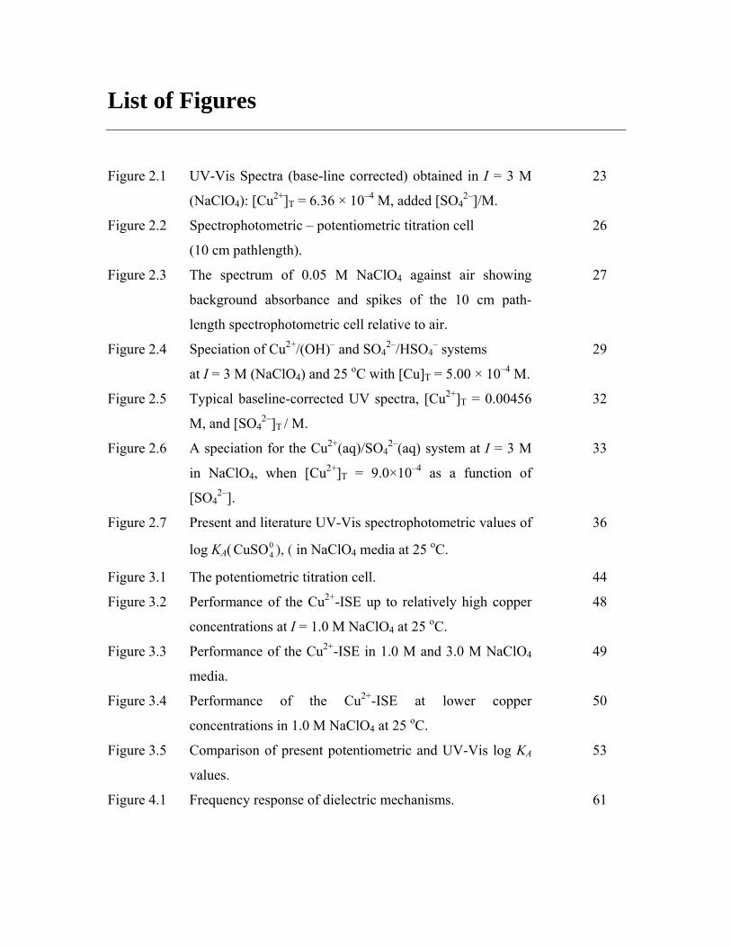
List of Figures
Figure 2.1 UV-Vis Spectra (base-line corrected) obtained in I = 3 M
(NaClO4): [Cu2+]T = 6.36 × 10⁻⁴ M, added [SO42–]/M.
23
Figure 2.2 Spectrophotometric – potentiometric titration cell
(10 cm pathlength).
26
Figure 2.3 The spectrum of 0.05 M NaClO4 against air showing
background absorbance and spikes of the 10 cm path-
length spectrophotometric cell relative to air.
27
Figure 2.4 Speciation of Cu2+/(OH)– and SO42–/HSO4
– systems
at I = 3 M (NaClO4) and 25 oC with [Cu]T = 5.00 × 10⁻⁴ M.
29
Figure 2.5 Typical baseline-corrected UV spectra, [Cu2+]T = 0.00456
M, and [SO42–]T / M.
32
Figure 2.6 A speciation for the Cu2+(aq)/SO42–(aq) system at I = 3 M
in NaClO4, when [Cu2+]T = 9.0×10⁻⁴ as a function of
[SO42–].
33
Figure 2.7 Present and literature UV-Vis spectrophotometric values of
log KA( ), ( in NaClO4 media at 25 oC. 04CuSO
36
Figure 3.1 The potentiometric titration cell. 44
Figure 3.2 Performance of the Cu2+-ISE up to relatively high copper
concentrations at I = 1.0 M NaClO4 at 25 oC.
48
Figure 3.3 Performance of the Cu2+-ISE in 1.0 M and 3.0 M NaClO4
media.
49
Figure 3.4 Performance of the Cu2+-ISE at lower copper
concentrations in 1.0 M NaClO4 at 25 oC.
50
Figure 3.5 Comparison of present potentiometric and UV-Vis log KA
values.
53
Figure 4.1 Frequency response of dielectric mechanisms. 61
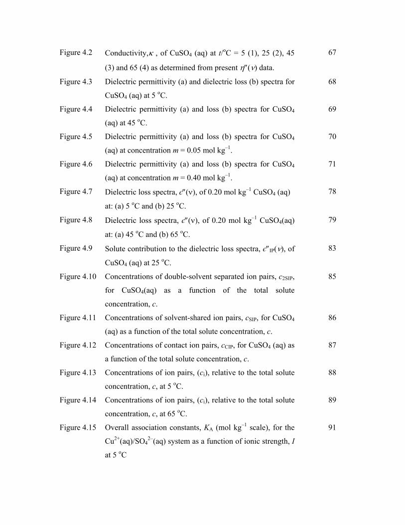
Figure 4.2 Conductivity,κ , of CuSO4 (aq) at t/oC = 5 (1), 25 (2), 45
(3) and 65 (4) as determined from present η″(ν) data. 67
Figure 4.3 Dielectric permittivity (a) and dielectric loss (b) spectra for
CuSO4 (aq) at 5 oC. 68
Figure 4.4 Dielectric permittivity (a) and loss (b) spectra for CuSO4
(aq) at 45 oC. 69
Figure 4.5 Dielectric permittivity (a) and loss (b) spectra for CuSO4
(aq) at concentration m = 0.05 mol kg–1. 70
Figure 4.6 Dielectric permittivity (a) and loss (b) spectra for CuSO4
(aq) at concentration m = 0.40 mol kg–1. 71
Figure 4.7 Dielectric loss spectra, є″(ν), of 0.20 mol kg–1 CuSO4 (aq)
at: (a) 5 oC and (b) 25 oC.
78
Figure 4.8 Dielectric loss spectra, є″(ν), of 0.20 mol kg–1 CuSO4(aq)
at: (a) 45 oC and (b) 65 oC. 79
Figure 4.9 Solute contribution to the dielectric loss spectra, є″IP(ν), of
CuSO4 (aq) at 25 oC. 83
Figure 4.10 Concentrations of double-solvent separated ion pairs, c2SIP,
for CuSO4(aq) as a function of the total solute
concentration, c.
85
Figure 4.11 Concentrations of solvent-shared ion pairs, cSIP, for CuSO4
(aq) as a function of the total solute concentration, c. 86
Figure 4.12 Concentrations of contact ion pairs, cCIP, for CuSO4 (aq) as
a function of the total solute concentration, c. 87
Figure 4.13 Concentrations of ion pairs, (ci), relative to the total solute
concentration, c, at 5 oC. 88
Figure 4.14 Concentrations of ion pairs, (ci), relative to the total solute
concentration, c, at 65 oC.
89
Figure 4.15 Overall association constants, KA (mol kg–1 scale), for the
Cu2+(aq)/SO42–(aq) system as a function of ionic strength, I
at 5 oC
91
Figure 4.16 Gibbs energy change ΔGo, for the ion association reaction
(Equation 1.24) for CuSO4(aq) as a function of
temperature, T.
93
Figure 4.17 Stepwise stability constants Ki for the formation of the ion-
pair types for Cu2+(aq)/SO42–(aq) system at 25 oC.
95
Figure 4.18 Stepwise stability constants Ki for the formation of the ion-
pair types for Cu2+(aq)/SO42–(aq) system at 5 oC.
96
Figure 4.19 Stepwise stability constants Ki for the formation of the ion-
pair types for Cu2+(aq)/SO42–(aq) system at 45 oC.
97
Figure 4.20 Stepwise stability constants Ki for the formation of the ion-
pair types for Cu2+(aq)/SO42–(aq) system at 65 oC.
98
Figure 4.21 Solute relaxation times τ1, τ2 and τ3 for CuSO4(aq) at
temperatures t/oC = 5, 25, 45, and 65.
100
Figure 4.22 Effective hydration numbers, Zib(CuSO4(aq)) at
temperatures t/oC = 5(1), 25(2), 45(3) and 65(4).
102
Figure 4.23 Effective hydration numbers at 25 oC. 104
Figure 5.1 Functional diagram of the TAM. 112
Figure 5.2 Detection and measurement system of the TAM. 114
Figure 5.3 Thermogram for 0.2 M Cu2+ in NaClO4 titrated into 0.2 M
Na2SO4 in NaClO4 (measuring the heat of reaction) or into
NaClO4 only (measuring the heat of dilution) at I = 3 M
(Method A).
117
Figure 5.4 Thermogram for 0.2 M SO42– in NaClO4 titrated into 0.2 M
Cu(ClO4) 2 in NaClO4 (measuring the heat of reaction) or
into NaClO4 only (measuring the heat of dilution) at I = 3
M (Method B).
118
Figure 5.5 Observed heats of dilution as a function of constant ionic
back ground for Methods A () and B ().
123
Figure 5.6 Observed heats of reaction as a function of ionic strength
using Method A () and Method B (∆).
124
Figure 5.7 Enthalpy change for the formation of as a function
of ionic strength at 25 oC.
04CuSO 127
Figure 5.8 Enthalpy change for the formation of as a function
of ionic strength at 25 oC (SIT model).
04CuSO 130
Figure 5.9 The hydration enthalpy of M2+ ions of the first row of the d
block.
133
Figure 5.10 Standard enthalpy change for the formation of (aq)
complexes of the first row of the d block elements.
04MSO 134
Figure 6.1 Osmotic coefficient data for binary solutions of Na2SO4,
MgSO4 and CuSO4 at 25 oC.
151
Figure 6.2 Comparison of the isopiestic molalities of the Na2SO4-
CuSO4-H2O and Na2SO4-MgSO4-H2O systems at 25 oC
with Zdanovskii’s rule.
153
Figure 6.3 Comparison of the isopiestic molalities of the CuSO4-
MgSO4-H2O system at 25 oC with Zdanovskii’s rule.
154
Figure 6.4 Experimental densities of aqueous solutions of CuSO4,
MgSO4 and Na2SO4 at 25 oC.
157
Figure 6.5 Apparent molal volumes at 25 oC of Na2SO4(aq) plotted
against m .
159
Figure 6.6 Apparent molal volumes at 25 oC of CuSO4(aq) plotted
against m .
160
Figure 6.7 Apparent molal volumes at 25 oC of MgSO4(aq) plotted
against m .
161
Figure 6.8 Densities for the mixtures of Na2SO4-CuSO4, Na2SO4-
MgSO4 and CuSO4-MgSO4 at 25 oC.
162
Figure 6.9 Apparent molal volumes for CuSO4-Na2SO4 as a function
of Tm at 25 oC.
164
Figure 6.10 Heat capacities for Na2SO4, CuSO4 and MgSO4 obtained
from ‘first leg’ and ‘second leg’ measurements in a Picker
165
calorimeter as a function of molality.
Figure 6.11 Heat capacities at 25 oC (first leg measurements) for
Na2SO4, CuSO4 and MgSO4 as a function of molality.
166
Figure 6.12 Apparent molal heat capacities at 25 oC of Na2SO4(aq),
CuSO4(aq) and MgSO4(aq) solutions.
167
Figure 6.13 Heat capacities at 25 oC for CuSO4-Na2SO4 mixtures as a
function of ionic strength fraction.
168
Figure 6.14 Present solubility data for CuSO4 and MgSO4 in Na2SO4
media at 60 oC and 90 oC.
171
Figure 6.15 Dynamic viscosities, η, at 25 oC of aqueous mixtures of:
(CuSO4+Na2SO4), (MgSO4+Na2SO4) and
(CuSO4+MgSO4) as a function of ionic strength fraction,
yi.
174

Abbreviations and symbols
a activity of the solute
å mean distance of the closest approach of the ions
A Debye-Hückel constant
A absorbance
AL Debye Hückel parameter for enthalpies
Å angstrom (10–10 m)
AMD acid mine drainage
aq aqueous
AR analytical reagent
α polarisability
B second Debye-Hückel constant
α, β empirical exponents for Equation 4.8
b cell path-length
BL Beer-Lambert law
B, C, D adjustable parameters
c concentration
ci concentration of the species i
ca. circa
cal calorimetry
CIP contact ion-pair oC degrees Celsius
appsc apparent water concentration
osc analytical (total) concentration of water
pc heat capacity
pφC apparent molar heat capacities
CN+, CN– sum of the first-shell coordination numbers
Cu2+-ISE copper ion selective electrode
3D three Debye
D-H Debye-Hückel
DRS dielectric relaxation spectroscopy
ΔHo standard enthalpy change
ΔS entropy change
e electronic charge
Eobs observable cell potential
Eind, Eref potentials of the indicator and reference electrodes
Ej potentials of any liquid junctions
),( kiε empirical ion interaction coefficient
ESTA Equilibrium Simulation for Titration Analysis
ε dielectric constant
ε(ν) complex dielectric permittivity
ε′(ν) dielectric dispersion
ε″(ν) dielectric loss
∞ε infinite frequency permitivity
ελ absorptivity at wavelength λ
εs low frequency permittivity
F Faraday’s constant (9.6487 x 10⁴ coulombs per mole)
fIP field factor
G Gibbs energy
GHz giga hertz
g gram
gl glass electrode
γ activity coefficient
γ+ activity coefficient
γ– activity coefficient
γ± mean ionic activity coefficient
h hour
Hz hertz
I ionic strength
IP ion-pair
ISE ion-selective electrode
IT , II monochromatic radiant power transmitted by, and
incident upon, the medium.
k kilo-, 103 (as in kg)
k Boltzmann constant
κ conductivity
κe effective conductivity
KA overall ion association constant oAK standard ion association constant
K1, K2, K3 stepwise association constants Kout outer sphere complex Kin inner sphere complex
λ wavelength
L1 relative partial molar enthalpy of water
l length of the constant-bore capillary
L litre (cubic decimeter, dm–3)
Ln– anion
ln natural logarithm
LJP liquid junction potential
M molar (mol/L solution)
Mm+ cation
m milli-, 10–3 (as in mL)
m metre
m molal (mol/kg solvent)
MHg mercury amalgam electrode
m*, im′ equilibrium molalities of the reference and sample
mol mole
n general number
n Number of electrons involved in the electrochemical
reaction
N total number of titration points
NA Avogadro’s number ne number of parameters to be optimised
Nc number of ligands specified in the SPECFIT model
np total number of electrodes
η viscosity
OBJE objective function
p indicates negative log (as in pH, pK)
p number of metal ions present in a particular species
p Pico-, 10–12 (as in ps)
Pa pascal
pH –log[H+]
ppm parts per million
PTFE polytetrafluoroethylene
π pi constant: 3.14159 *φ , φ osmotic coefficients of the reference and the mixed-
electrolyte solution
)(tPr
time-dependent electric polarization
μPr
, orientational polarization
αPr
induced polarization
q arbitrary distance
Qc heat of complexation
Qr heats of reaction
Qd heats of dilution
r ionic radius
r number of moles of water
r2 correlation coefficient
R universal gas constant (8.314 J K–1 mol–1)
r radius of the constant-bore capillary
σ experimental standard deviation
ρ, ρo density of an electrolyte solution, and the pure solvent
SIP solvent-shared ion-pair
σp standard deviation
2SIP double solvent-separated ion-pair
SIT specific ion interaction theory
Sj Dispersion amplitude
s second
(s) solid
Sol solubility
s2 variance
SD standard deviation
T thermodynamic temperature (in Kelvin, K)
t Temperature (in Celsius, oC)
τ dielectric relaxation time
µ Micro-, 10–6 (as in µm) 2τ vibration period of the tube
µ dipole moment
µ chemical potential of a solute
µo standard potential of a solute
IPμ dipole moments
U objective function
V volt
V Partial molal volume
V total volume
VNA vector network analyser
ν frequency
φV apparent molal volumes
ν* ,νi stoichiometric ionization numbers
ω field frequency
W watts
w mass
oW baseline power applied to the cells
[X] concentration of species X
yi ionic strength fraction
zi charge on species i
+z charge number of the cation
−z charge number of the anion
ZIB effective solvation number
179
Appendix
( ) ( )[ ]cacaaa
aac
i 32
23
21 expexp −−−×−
= (S1)
( )( )
−+
−×+−+−×+×
+−−−×=
243
243432
43
321
)exp()()(exp1exp1
aaa
caaacaaa
aa
acaac
i (S2)
−×=
2
3
21
)/ln(
2
1exp
a
acac
i (S3)
1
Chapter One
Introduction
1.1 THE IMPORTANCE OF CuSO4 SOLUTIONS
Aqueous solutions of copper(II) sulfate have an extensive range of agricultural,
environmental, industrial and hydrometallurgical uses. For example, copper sulfate
solution has been used in the agriculture industry to prepare Bordeaux (CuSO4, lime and
water) and Burgundy (CuSO4, Na2CO3) mixtures for controlling fungal diseases [82H,
83W], in the manufacture of insecticides and herbicides [83HK], and for correction of
copper deficiency in soils and animals [79N, 90B]. It has also been used as a disinfectant
against storage rots and for the control and prevention of certain animal diseases such as
foot rot in sheep and cattle because of its fungicidal and bactericidal properties [82H, 04K].
In an environmental context, copper(II) sulfate solution has been used to control algal
growth in water supplies and tadpole shrimps in flooded rice fields [79N]. Very dilute
solutions of copper sulfate are used to treat aquarium fish for various parasitic infections
[04K]. In the photographic industry, copper(II) sulfate solution is used as a mordant bath
for intensifying photographic negatives and as a reagent toner [04K]. It is also used as a
base chemical for the production of a number of other copper compounds (e.g. copper
napthenate, copper soap). In the synthetic fibre industry, CuSO4 solution is applied in the
production of various raw materials, while in the paint industry it is used in anti-fouling
paints, as well as for colouring glass and in dyes and pigments [07Aa]. In
analytical/medical chemistry, copper(II) sulfate solution is a component of Fehling’s and
Benedict’s solutions to test for reducing sugars, as Biuret reagent to test for protein and to
test blood anaemia [07Aa]. Other applications of copper(II) sulfate solution include
battery electrolytes, copper ‘sweetening’ in petroleum refining, pyrotechnics, corrosion
inhibitors, froth floatation agents for lead, zinc, cobalt and gold ores, laundry and metal
marking ink and also as a fuel additive [07Aa]. In summary, it is probably fair to say that,
2
there is hardly any industry that does not have some use for an aqueous solution of
copper(II) sulfate.
However, the major use of copper(II) sulfate solutions is in the minerals industry where it
is a key intermediate in the recovery of copper from its ores, in copper refining and in
copper electroplating processes [94BD]. This usage provided the most important
motivation for the work described in this thesis. It is accordingly appropriate to discuss
briefly here the occurrence of copper minerals and the methods used for the extraction of
copper from them.
1.2 COPPER MINERALS
1.2.1 Occurrence
Copper has been an important metal from as early as 5000 BC [76T] and has a wide
variety of useful properties. It is reasonably abundant in the Earth’s crust (68 ppm) being
far higher than the other coinage metals silver (0.08 ppm) and gold (0.004 ppm) [04K].
The most common forms of copper present in crustal rocks are copper-iron sulfides, such
as chalcopyrite (CuFeS2) and bornite (Cu5FeS2), and straight copper sulfides such as
chalcocite, Cu2S. Copper also occurs to a lesser extent in oxidized forms such as
carbonates (Cu2CO3(OH)2), oxides, hydroxysilicates and sulfates [94BD].
Like most metals, copper is in general not sufficiently concentrated in its ore bodies to
allow direct smelting. Economically feasible mining methods are selected according to the
nature and concentration of minerals in the ore body. Underground mining is used when
the typical ore contains about 1 or 2% copper whereas open pit mining is selected when
ores contain ≤ 0.5% copper [94BD].
Copper ore minerals are classified as primary (minerals concentrated in ore bodies by
hydrothermal processes), secondary (minerals formed when copper sulfides are oxidized)
or as native copper. The process used for copper extraction is selected according to the
3
nature of the copper ore minerals but in practice invariably involves the formation, at some
stage, of copper(II) sulphate solutions.
1.2.2 Pyrometallurgical extraction
Pyrometallurgical methods are typically used to extract copper from ores containing
copper-iron-sulphide minerals because of the difficulties in dissolving these minerals in
aqueous solutions. The initial step of this method is the isolation of copper mineral
particles from the other impurities by froth flotation. The isolated (floated) fraction
typically contains 25 – 35% copper, which is then smelted to produce concentrated molten
copper-rich ‘matte’. This molten ‘matte’ is then transferred to converters for oxidation to
blister copper. The blister copper is electrochemically refined to high purity cathode
copper using a CuSO4-H2SO4-H2O electrolyte. In this process the impure copper is
electrochemically dissolved at the anode and pure copper is electroplated onto copper or
stainless steel cathodes [94BD].
1.2.3 Hydrometallurgical extraction
Direct hydrometallurgical extraction is used to obtain copper from ores containing oxidised
copper minerals such as carbonates, hydroxysilicates, sulfates and hydroxychlorides
[94BD]. Hydrometallurgical extraction typically involves three steps: a) sulfuric acid
leaching of crushed copper-containing ore or mine waste to produce an impure copper-
bearing aqueous solution, b) solvent extraction of the solution followed by back-extraction
to produce a pure, high-copper aqueous electrolyte solution (CuSO4(aq)), and c)
electrolysis of this solution to produce pure electroplated cathode copper.
1.3 COPPER(II) SULFATE SOLUTIONS
Copper(II) sulfate pentahydrate, CuSO4·5H2O, which occurs in nature as the mineral
chalcanthite, is the most common commercial product of copper and is produced
industrially in the form of blue triclinic crystals [04K]. It has solubility in aqueous
solution varying from 24.3 g/100 mL (0 oC) to 205.0 g/100 mL (100
oC) [07Ab].
4
Copper(II) sulfate solution is also produced from copper scraps, blister copper, copper
precipitates, electrolytic refinery solutions and spent electroplating solutions, as well as
from a variety of copper containing liquors using solvent extraction for purification
[94BD]. However, the most common commercial method of preparing CuSO4 solution is
the aeration or oxygenation of hot dilute aqueous sulfuric acid in the presence of copper
metal.
Due to the widespread applications of copper sulfate, both alone and when mixed with
other substances (Sections 1.1 & 1.3), the determination and correct interpretation of the
thermodynamic data related to the Cu2+
/SO42–
interaction is necessary for a better
understanding of the impact of copper(II) sulfate in biological and industrial systems. As
the present work is concerned with thermodynamic and related studies of aqueous
copper(II) sulfate solutions, it is appropriate to review briefly the fundamental theories of
ions in aqueous solution.
1.4 THEORIES OF IONIC SOLUTIONS
Various theories have been used to describe aqueous solutions of electrolytes. The first
major breakthrough in understanding the nature of electrolyte solutions came from
Arrhenius who developed the theory of electrolyte ionization in aqueous solutions [66N].
The obvious deficiencies in Arrhenius’s original ideas led to the development of other
theoretical approaches such as the ion-interaction, mean salt and ion-hydration theories
[90MB]. For example, Brønsted [22B] developed his theory of specific ion interaction,
which was based on the approximation that significant chemical interactions in electrolyte
solutions are limited to those between ions of opposite sign. In 1923 the first statistical
theory of electrolyte solutions, the inter-ionic attraction theory developed by Debye and
Hückel, was successful in interpreting the behaviour of very dilute solutions. The Debye-
Hückel theory assumes that electrolytes are completely ionized, takes into account only the
long range electrostatic interactions that occur between ions, and considers the solvent as a
dielectric continuum. However, this theory failed even in slightly concentrated electrolyte
solutions [86ZCR].
5
In solution, the chemical potential of a solute can be expressed [90A] as
aRTµµ lno+= (1.1)
where oµ is the standard chemical potential of the solute, R is the universal gas constant
(8.314 J K–1
mol–1
), T is the thermodynamic temperature (in Kelvin, K) and a is the
activity of the solute. The activity of a solute is related to its concentration c by
cγa ⋅= (1.2)
where γ is the activity coefficient. Inserting Equation 1.2 into Equation 1.1 gives
γcRTµµ lno+= (1.3)
and thus
γRTcRTµµ lnlno++= (1.4)
Written in this way it is clear that γ describes the non-ideal behaviour of the solution,
which is related to the interactions occurring between the solute particles. By definition,
the value of γ tends towards unity (γ → 1 as c → 0) in very dilute solutions (where the
interactions between solute particles approach zero) [70RS, 94KR].
Equations 1.1 to 1.4 are true for any solute dissolved in any solvent, at equilibrium.
However, there is a complication for electrolyte solutions. While the concentration of an
individual cation or anion in a solution has a clear meaning, it is impossible within the
framework of thermodynamics to assign one part of the non-ideality of a solution to the
cation and the other part to the anion. Only the mean ionic activity coefficient of the salt,
γ± can be measured where
21 /)(−+±
= γγγ (1.5)
6
The activity coefficients of the individual cations and anions, γ+ and γ–, respectively cannot
be measured. Equation 1.4 for an electrolyte must thus be written as
±++= γRTcRTµµ lnlno (1.6)
The long range and strength of the coulombic interactions between ions is the primary
reason why electrolyte solutions show departures from ideal solution behaviour even at
very low concentrations. Such interactions are considered to dominate the other
contributions to non-ideality [90A] in low or moderately concentrated solutions.
These long-range coulombic forces can be modelled at very low concentrations by the
Debye-Hückel limiting law, which can be used to calculate the mean activity coefficient
under such conditions.
IzzA ||log −+± −=γ (1.7)
in which A is generally referred to as the Debye-Hückel constant. This quantity can be
derived theoretically purely in terms of known quantities (Equation 1.8). It has a value of
0.5100/(mol–1/2
kg1/2
) for an aqueous solution at 25 oC [97GP]. The terms z+ and z– are the
charge numbers (corresponding to the valence) of the cation and anion respectively. In
Equation 1.7, I is the ionic strength of the solution ( 2
21
iizcI ∑= , where ci is the
concentration of the species i with charge zi).
As already noted, the Debye-Hückel constant for activity coefficients A can be calculated
from fundamental constants [70RS]
1000
2
2.303
1 AN
kT
eA
π
ε=
3
3
(1.8)
where e is the electronic charge, NA is Avogadro’s number, ε is the dielectric constant, k is
the Boltzmann constant [86ZCR] and other symbols have their usual meanings.
7
According to Equation 1.7, log γ± should decrease linearly with the square root of
increasing ionic strength. However it is known the Debye-Hückel limiting law is valid
only for very dilute solutions (c 10–3
M). Experimental results show that ±
γlog
generally passes through a minimum and then increases at higher I, although the exact
shape of the curve and the location of the minimum depend on the nature of the dissolved
salt [70RS]. It follows that the Debye-Hückel limiting law equation (1.7) requires
modification to describe solutions with appreciable electrolyte concentrations [72GP].
Initially, an additional term which takes the finite sizes of the ions into account was
introduced in an attempt to extend the theory to higher concentrations. This expression is
often called the ‘extended’ Debye-Hückel theory and has the form:
IBå
IzzA
1
||log
+−= −+
±γ (1.9)
where å is the mean distance of closest approach of the ions in the solution and varies with
the nature of the ions. The B term is sometimes known as the second Debye-Hückel
constant for activity coefficients and can, again, be calculated from fundamental quantities
[70RS]:
εkT
eNB
1000
8 A
2π
= (1.10)
where the symbols have same meanings as in Equation 1.8.
Equation 1.9 can be used to estimate the activity coefficient of ionic solutions with higher
concentrations (c 0.01 M) [90A] but still predicts an ongoing decrease in ±
γlog with
increasing I since
B
A
IB
IA
′
′→
′+
′
1 as ∞→I
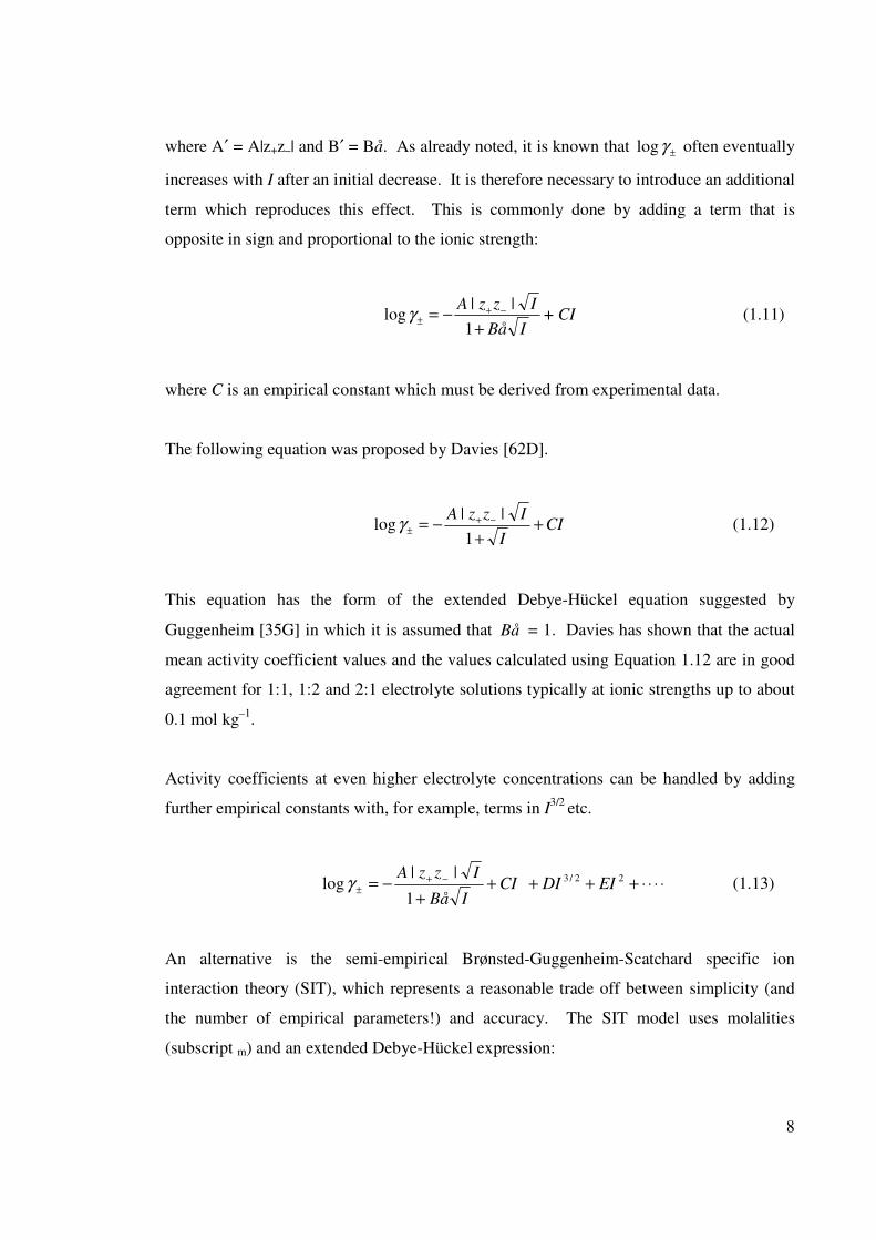
8
where A′ = A|z+z–| and B′ = Bå. As already noted, it is known that ±
γlog often eventually
increases with I after an initial decrease. It is therefore necessary to introduce an additional
term which reproduces this effect. This is commonly done by adding a term that is
opposite in sign and proportional to the ionic strength:
IBå
IzzA
+−= −+
±1
||logγ + CI (1.11)
where C is an empirical constant which must be derived from experimental data.
The following equation was proposed by Davies [62D].
CI
I
IzzA+
+−= −+
±1
||logγ (1.12)
This equation has the form of the extended Debye-Hückel equation suggested by
Guggenheim [35G] in which it is assumed that Bå = 1. Davies has shown that the actual
mean activity coefficient values and the values calculated using Equation 1.12 are in good
agreement for 1:1, 1:2 and 2:1 electrolyte solutions typically at ionic strengths up to about
0.1 mol kg–1
.
Activity coefficients at even higher electrolyte concentrations can be handled by adding
further empirical constants with, for example, terms in I3/2
etc.
⋅⋅⋅⋅+++++
−= −+
±
22/3
1
||log EIDICI
IBå
IzzAγ (1.13)
An alternative is the semi-empirical Brønsted-Guggenheim-Scatchard specific ion
interaction theory (SIT), which represents a reasonable trade off between simplicity (and
the number of empirical parameters!) and accuracy. The SIT model uses molalities
(subscript m) and an extended Debye-Hückel expression:
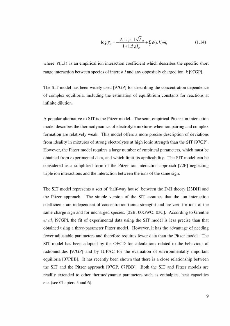
9
kk
m
mmki
I
IzzA),(
5.11
||log εγ Σ+
+−= −+
± (1.14)
where ),( kiε is an empirical ion interaction coefficient which describes the specific short
range interaction between species of interest i and any oppositely charged ion, k [97GP].
The SIT model has been widely used [97GP] for describing the concentration dependence
of complex equilibria, including the estimation of equilibrium constants for reactions at
infinite dilution.
A popular alternative to SIT is the Pitzer model. The semi-empirical Pitzer ion interaction
model describes the thermodynamics of electrolyte mixtures when ion pairing and complex
formation are relatively weak. This model offers a more precise description of deviations
from ideality in mixtures of strong electrolytes at high ionic strength than the SIT [97GP].
However, the Pitzer model requires a large number of empirical parameters, which must be
obtained from experimental data, and which limit its applicability. The SIT model can be
considered as a simplified form of the Pitzer ion interaction approach [72P] neglecting
triple ion interactions and the interaction between the ions of the same sign.
The SIT model represents a sort of ‘half-way house’ between the D-H theory [23DH] and
the Pitzer approach. The simple version of the SIT assumes that the ion interaction
coefficients are independent of concentration (ionic strength) and are zero for ions of the
same charge sign and for uncharged species. [22B, 00GWO, 03C]. According to Grenthe
et al. [97GP], the fit of experimental data using the SIT model is less precise than that
obtained using a three-parameter Pitzer model. However, it has the advantage of needing
fewer adjustable parameters and therefore requires fewer data than the Pitzer model. The
SIT model has been adopted by the OECD for calculations related to the behaviour of
radionuclides [97GP] and by IUPAC for the evaluation of environmentally important
equilibria [07PBB]. It has recently been shown that there is a close relationship between
the SIT and the Pitzer approach [97GP, 07PBB]. Both the SIT and Pitzer models are
readily extended to other thermodynamic parameters such as enthalpies, heat capacities
etc. (see Chapters 5 and 6).
10
1.5 ION PAIRING
1.5.1 Formation of ion pairs
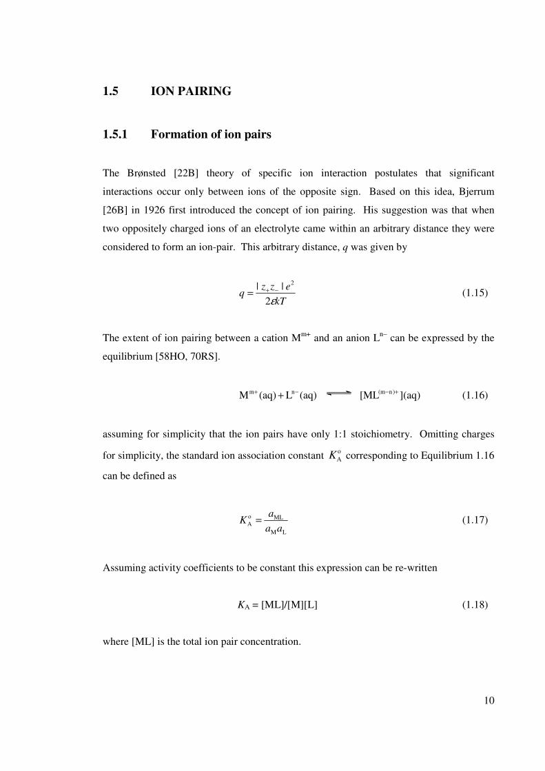
The Brønsted [22B] theory of specific ion interaction postulates that significant
interactions occur only between ions of the opposite sign. Based on this idea, Bjerrum
[26B] in 1926 first introduced the concept of ion pairing. His suggestion was that when
two oppositely charged ions of an electrolyte came within an arbitrary distance they were
considered to form an ion-pair. This arbitrary distance, q was given by
kT
ezzq
ε2
||2
−+= (1.15)
The extent of ion pairing between a cation Mm+
and an anion Ln–
can be expressed by the
equilibrium [58HO, 70RS].
(aq)L(aq)M nm −++ ](aq)[ML )n(m +− (1.16)
assuming for simplicity that the ion pairs have only 1:1 stoichiometry. Omitting charges
for simplicity, the standard ion association constant o
AK corresponding to Equilibrium 1.16
can be defined as
LM
MLo
Aaa
aK = (1.17)
Assuming activity coefficients to be constant this expression can be re-written
KA = [ML]/[M][L] (1.18)
where [ML] is the total ion pair concentration.
11
1.5.2 The Eigen-Tamm mechanism
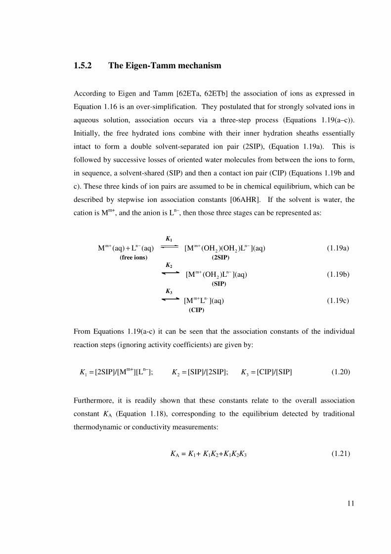
According to Eigen and Tamm [62ETa, 62ETb] the association of ions as expressed in
Equation 1.16 is an over-simplification. They postulated that for strongly solvated ions in
aqueous solution, association occurs via a three-step process (Equations 1.19(a–c)).
Initially, the free hydrated ions combine with their inner hydration sheaths essentially
intact to form a double solvent-separated ion pair (2SIP), (Equation 1.19a). This is
followed by successive losses of oriented water molecules from between the ions to form,
in sequence, a solvent-shared (SIP) and then a contact ion pair (CIP) (Equations 1.19b and
c). These three kinds of ion pairs are assumed to be in chemical equilibrium, which can be
described by stepwise ion association constants [06AHR]. If the solvent is water, the
cation is Mm+
, and the anion is Ln–
, then those three stages can be represented as:
K1
(aq)L(aq)M nm −++ ](aq))L)(OH(OH[M n
22
m −+ (1.19a)
(free ions) (2SIP) K2
](aq))L(OH[M n
2
m −+ (1.19b)
(SIP)
K3
](aq)L[M -nm+ (1.19c)
(CIP)
From Equations 1.19(a-c) it can be seen that the association constants of the individual
reaction steps (ignoring activity coefficients) are given by:
=1K [2SIP]/[Mm+
][Ln–
]; =2K [SIP]/[2SIP]; =3K [CIP]/[SIP] (1.20)
Furthermore, it is readily shown that these constants relate to the overall association
constant KA (Equation 1.18), corresponding to the equilibrium detected by traditional
thermodynamic or conductivity measurements:
KA = K1+ K1K2+K1K2K3 (1.21)
12
Although this overall scheme of ion association (Equations 1.19(a-c)) has been
demonstrated to occur for a number of salts [04BCH, 05CHB] this does not necessarily
mean that all steps (species) will be detectable in any given system.
In principle, any technique that can be used to study complex formation can also be used
for the investigation of ion pairing [06MH]. However, methods such as ultrasonic
[00KHE] and dielectric [01BB, 04B] relaxation have special capabilities for such studies
because they are the only techniques currently available that are capable of separately
determining the presence of all the types of ion pairs (Equations1.19(a-c)) in solution. In
this way a more detailed knowledge of the actual species present can be obtained.
Traditional methods such as conductometry and potentiometry do not distinguish between
the various types of ion pairs: they measure only the overall association KA. On the other
hand, most popular spectroscopic methods such as NMR, Raman and UV-Visible, usually
detect only the direct contact (CIP) species. Therefore, if the electrolyte solution contains
solvent separated ion pairs, the log KA value obtained from those studies may be lower
than the true value [06He]. The magnitude of the error involved depends on the system as
well as the method used.
This effect has not been well studied in respect of aqueous copper sulfate solutions and is
one of the main issues considered in this thesis.
1.6 ION ASSOCIATION STUDIES ON AQUEOUS Cu2+
/SO42–
1.6.1 Association constants
It has generally been accepted that CuSO4(aq) solutions, like those of the other divalent
sulfates, are appreciably associated at moderate salt concentrations [70RS]. If the
formation of species with different hydration levels (Equations 1.19(a-c)) is ignored, then
the overall association of copper(II) and sulfate ions
13
KA
Cu2+
(aq) + SO42–
(aq) 0
4CuSO (aq) (1.22)
appears to be the only significant equilibrium present in aqueous solutions of copper(II)
sulfate [07PBB].
Various techniques [07PBB] have been employed for the purpose of obtaining quantitative
association constants for aqueous solutions of copper(II) sulfate or related information
[70RS, 92ZA]. At least 78 publications (Table 1.1) containing quantitative information on
ion association are available for this system, half of them providing the log AK values at
infinite dilution (i.e. log o
AK ). In spite of this vast number of studies, the formation
constants reported for Equation 1.22 at infinite dilution (Table 1.1) show a surprisingly
large uncertainty, (1.9 ≤ log o
AK ≤ 2.8) for such an apparently simple system. This
suggests there are difficulties in quantifying this system, which has often been taken as a
paradigm for ion association studies [50F, 55BP, 70RS, 62D, 07PBB].
Thus, surprisingly, it cannot be said that the thermodynamics of complex formation of
Cu2+
(aq)/SO42–
(aq) system are as well characterized as might be expected from the large
number of reported studies. This statement is particularly true at finite ionic strengths
where almost all of the data have been obtained from spectroscopic studies in either
LiClO4 or NaClO4 media. Although the reported values are in reasonable agreement with
each other, as already noted above, such results may contain systematic errors arising from
the failure of UV-Vis spectroscopy to detect all of the ion pair types [06He].
On the basis of the many published studies (Table 1.1) it would appear that the
Cu2+
(aq)/SO42–
(aq) system can be considered as a modestly associated simple system
apparently forming only one complex (Equation 1.22) in an apparently straightforward
manner. The presence of competing reactions is clearly one cause of the difficulties
mentioned above. At higher pH (pH > 5), the hydrolysis reaction
+2
62 )Cu(OH++−
+ H(OH)Cu y)(2x
yx (1.23)
14
Table 1.1 Literature values of log KA at 25 oC [07PBB].
Medium/M
t/oC
Method log KAa References
0 corr 25 Conductivity 2.37 38OG
→0 25 Spectrophotometry 2.15 49Na
0 corr 25 Recalc(con) 2.34 ± 0.02 38OG/51W
0 corr 25 Spectrophotometry 2.33 ± 0.03 56BDM
0 corr 25 Spectrophotometry 2.10–2.46b 57DOP
0 corr 25 Recalc(con) 2.31–2.41b 38OG/57DOP
0 corr 25 Conductivity(high field ) 2.37 52BP/61PF
0 corr 25 Conductivity 2.28 38OG/62AY
0 corr 25 Conductivity(high field ) 2.32 62AY, 68YMK
0corr 25 Spectrophotometry 2.23–2.40b 65M
→0 25 (Dielectric relaxation) 1.93 65P
0 corr 25 Conductivity 2.25 65YK
→0 25 Spectrophotometry 2.35 68HP
0 corr 25 Recalc(act) 2.15–2.37b 69GG
0 corr 25 Calorimetry 2.26, 69IEC
→0 25 ultrasonic absorption 2.28 68HP/70HP
0 corr 25 Conductivity 2.12 69SM
0 corr 25 Recalc(con) 2.4 38OG/71HPP
→0 25 Spectrophotometry 2.26 71KVP
0 corr 25 Spectrophotometry 2.25 ± 0.01 71MKA
→0 25 Recalc(act, DH dil) 2.40 72P
→0 25 Recalc(con, act) 2.67 var/75T
0 corr 25 Spectrophotometry 2.19 ± 0.25 75YY
0 corr 25 Recalc(con) 2.13 ± 0.28 38OG/75YY
0 corr 25 Conductivity 2.8 77STK
0 corr 25 Recalc(con, sp) 2.29 38OG+75YY/81YY
0 corr 25 Spectrophotometry 2.32 ± 0.02, 82DKA
→0 25 Spectrophotometry 2.17 85LY
0 corr 25 Conductivity 2.31 ± 0.01 85SGZ
0 corr 25 Conductivity 2.35 ± 0.09 89MBR
0 corr 25 Spectrophotometry 2.24 ± 0.07 90GLY
→0 25 Recalc(spec, act) 2.19 90W
0 corr 25 Conductivity 2.2742 ± 0.0008 94NH
0 corr 25 Conductivity 2.43 00TM
0 corr 25 Conductivity 2.37 ± 0.02, 04RBP
(Cont’d)
b range corresponds to minor variants in the activity coefficient model adopted
15
Medium/M
t/oC
Method log KAa References
0.041 NaClO4 25 Spectrophotometry 1.64 65M
0.091 NaClO4 25 Spectrophotometry 1.38 65M
0.2 LiClO4 25 Spectrophotometry 1.21 85LY
0.2 NaClO4 25 Spectrophotometry 1.02 85LY
0.5 LiClO4 25 Spectrophotometry 0.84 49Nb
0.5 LiClO4 25 Spectrophotometry 0.96 85LY
0.5 NaClO4 25 Spectrophotometry 0.8 49Nb
0.5 NaClO4 25 Spectrophotometry 0.77 85LY
0.5 NaClO4 25 Spectrophotometry 0.9 90GLY
1.0 LiClO4 25 Spectrophotometry 0.75 85LY
1.0 LiClO4 25 Spectrophotometry 0.81 71KVP
1.0 NaClO4 20 MHg 1.03, β2= 0.10,
β3 = 1.17
48F
1.0 NaClO4 20 Spectrophotometry 0.63–0.65 48F/70SW
1.0 NaClO4 20 qh 0.95 50F
1.0 NaClO4 20 Sol, gl 1.04, β2 ~ 0.5,
β3 2.18
51NL
1.0 NaClO4 25 Spectrophotometry 0.66 49Nb
1.0 NaClO4 25 Polarography <0.5, β2 = 1.5 65TSO
1.0 NaClO4 25 Spectrophotometry 0.58, 77AH, 77AHa
1.0 NaClO4 25 Spectrophotometry 0.62 85LY
1.0 NaClO4 25 Spectrophotometry 0.74 90GLY
2.0 LiClO4 25 Spectrophotometry 0.73 49Nb
2.0 LiClO4 25 Spectrophotometry 0.60 ± 0.02 77KFT
2.0 LiClO4 25 Spectrophotometry 0.62 85LY
2.0 NaClO4 25 Spectrophotometry 0.61 49Nb
2.0 NaClO4 25 Calorimetry 0.59 ± 0.03, 69BG
2.0 NaClO4 25 Calorimetry 0.64 ± 0.02, 79GCE
2.0 NaClO4 25 Spectrophotometry 0.54 85LY
2.0 NaClO4 25 Spectrophotometry 0.63 90GLY
3.0 LiClO4 25 Spectrophotometry 0.83 49Nb
3.0 LiClO4 25 Spectrophotometry 0.38 ± 0.04 53N
3.0 LiClO4 25 Spectrophotometry 0.70, Kin = 0.5,
Kout = 0.67
68MMM,70MMM,
71KVP
3.0 LiClO4 25 Calorimetry 0.66, 70MMM, 74BRM
3.0 LiClO4 25 Spectrophotometry 0.68 85LY
3.0 NaClO4 25 Spectrophotometry 0.66 49Nb
3.0 NaClO4 25 Spectrophotometry 0.73 71KVP
3.0 NaClO4 25 Spectrophotometry 0.45, 77AH, 77AHa
3.0 NaClO4 25 Spectrophotometry 0.63 85LY
3.0 NaClO4 25 Spectrophotometry 0.69 90GLY
4.0 LiClO4 25 Spectrophotometry 0.52 ± 0.04, 77KFT
4.0 LiClO4 25 Spectrophotometry 0.77 85LY
5.0(unknown) 25 Spectrophotometry 0.9 71KVP
5 0NaClO4 25 Spectrophotometry 0.62, 77AH, 77AHa
a Refers to KA unless otherwise specified. β2 and β3 are overall formation constants.
Kin and Kout are inner- and outer-sphere complexes
16
will affect the apparent formation constant of equilibrium (1.22) and at low pH (pH < 4)
bisulfate formation
+−+ HSO 2
4
−
4HSO (1.24)
can compete with Cu2+
for SO42–
. Thus a proper study of the Cu2+
(aq)/SO42–
(aq) system
requires careful pH control of the solutions to avoid these complicating equilibria
(Equations 1.23 & 1.24).
As mentioned before, the available data (Table 1.1) mostly refer to infinite dilution and
there is a lack of high quality data relevant to typical industrial conditions of temperature
and ionic strengths. Formation constants of 0
4CuSO at infinite dilution are of limited use
for modelling the solutions used in practical processes because of the large changes in AK
that may occur at higher ionic strengths due to the changes in activity coefficients (see
Equations 1.7 to 1.14).
1.6.2 Enthalpy and entropy values
For modelling purposes, especially in industrial or environmental situations where
conditions of ionic strength and temperature may differ considerably from the standard
conditions of infinite dilution and 25 oC, it is essential to know how the formation constant
varies with these conditions. With regard to temperature this can be achieved by
measuring KA as a function of temperature. However, it is well established that a better,
more reliable, and easier approach is to measure the corresponding enthalpy (and entropy)
changes for the equilibrium. Theses quantities can then be used to calculate KA(T) via
standard thermodynamic relationships (see Chapter 5).
The enthalpy change associated with complex formation in the Cu2+
(aq)/SO42–
(aq) system
has been studied (Table 1.2) using various techniques. The data in Table 1.2 show that
∆Ho at infinite dilution is moderately well characterized by calorimetry and by direct
measurements of the variation of KA with temperature (the ‘K(T)’ or van’t Hoff method).
17
The various calorimetric studies on the Cu2+
(aq)/SO42–
(aq) system [69BG, 69IEC, 70L,
73HP, 73P] used three methods which are similar but which differ in important ways.
These differences are (a) the simultaneous determination of KA and ∆H by titration
calorimetry – the so-called 'entropy titration' technique – [69BG, 69IEC, 73P], (b) the
determination of ∆H alone calculated from calorimetric titration data using an
independently determined KA value, [73P, 73HP] and (c) heat of dilution measurements
[70L, 72P].
In contrast to the plethora of ∆Ho values obtained from measurements in dilute solutions,
there is only one study of ∆H as function of I [77AH, 77AHa]. Unfortunately, this study
employed the K(T) method, which is generally considered to be less reliable than direct
calorimetric measurements due to the errors involved in taking the derivative of the log KA
against 1/T plot [57N] and the presence of unsuspected temperature-dependent errors in
K(T) [06MH].
Table 1.2 Literature data for the enthalpy change for the reaction
Cu2+
(aq) + SO42–
(aq) → 0
4CuSO (aq) at 25 oC.
Method
I / M (NaClO4)
∆∆∆∆H / kJ mol–1
References
cal
cala
cala
cal
cal
K(T)
K(T)
K(T)
K(T)
cal
K(T)
K(T)
0 corr
0 corr
0 corr
0 corr
0corr
0 corr
0 corr
0 corr
1
2
3
5
5.1
7.2
6.7
10.2
9.5
7.7
6.5
6.4
9.9
7.3
5.9
2.2
69IEC
70L
72P
73HP
73P
82DKA
04RBP
05MBP
77AH/77AHa
69BG
77AH/77AHa
77AH/77AHa
aRecalculation of data from 69IEC
18
There is, therefore, virtually no reliable information on the ionic strength dependence of
∆H and ∆S for the Cu2+
(aq)/SO42–
(aq) system. Thus, a thorough investigation of the effects
of ionic strength dependence of ∆H was undertaken (see Chapter 5).
1.7 PROPERTIES OF CuSO4 IN MIXED-ELECTROLYTE
SYSTEMS
Although CuSO4(aq) solutions are important in their own right (Section 1.1) it is also
common in practical situations for CuSO4 to be present in mixed electrolyte solutions.
Industrial solutions such as those produced during some hydrometallurgical processes, not
only contain high concentrations of CuSO4 but also the sulfates of other metals such as Ni,
Co, Mg and Al. Similarly, run off from acid mine drainage also contains mixtures of
electrolyte solutions. Knowledge of the thermodynamic properties of these mixed
electrolyte solutions is required for understanding or modelling many phenomena in
industrial, geochemical, biological and environmental settings [90MB].
For example, the solutions produced by the high pressure acid leaching of nickel laterites
for the production of nickel and cobalt are essentially mixtures of metal sulfates. These
dissolved metal sulfates obviously interact with each other in complex ways and this can,
for example, have a significant impact on their mutual solubility as well as on the overall
efficiency of production. Copper(II) sulfate enters into the extraction process from the raw
ores and can become a significant contaminant [96R]. The same is true for processes used
for extracting for metals such as zinc and magnesium.
Acid mine drainage (AMD) is a serious environmental problem in the mining industry. It
occurs as a result of the interaction of ground water with metal sulphide-containing ore
bodies. Depending on the particular geochemistry and hydrology of the individual mine-
sites, these solutions comprise mostly mixtures of CuSO4/H2SO4 and FeSO4/H2SO4. As
concentrations can be quite high, such AMD solutions can cause serious pollution in the
environment. Understanding the species present in these AMD solutions and their
physicochemical properties such as density, heat capacity, solubility and viscosity is
19
helpful in designing methods to reduce the contamination levels before discharged into the
environment.
The physicochemical properties of copper(II) sulfate binary solutions (i.e. those consisting
of only the electrolyte dissolved in the solvent) have been well investigated. Large
amounts of data exist for activity coefficients, densities, heat capacities, solubilities and
many other thermodynamic quantities, as well as transport properties such as
conductivities and viscosities [99RC, 04M,]. However, data on the physicochemical
properties of copper(II) sulfate mixed with other divalent metal sulfates in mixtures of
ternary solutions (i.e. those consisting of two electrolytes dissolved in one solvent) are
scarce and are often of poor quality. Therefore, a detailed study of physicochemical
properties, osmotic coefficient, apparent molar volumes, heat capacities, densities and
solubilities of aqueous CuSO4 mixed with other electrolytes such as Na2SO4, and MgSO4
were undertaken here (Chapter 6) because of their usefulness in understanding chemical
speciation leading to further improvement of these chemical processes and method
development.
1.8 OVERVIEW OF THIS RESEARCH
The overall aim of the work described in this project has been to clarify the properties of
aqueous copper(II) sulfate solution, so that they can be better used in the many practical
applications where such solutions are involved. This thesis reports a detailed investigation
of ion association in the Cu2+
(aq)/SO42–
(aq) system. Since the majority of previous studies
of KA at high ionic strengths are from spectrophotometry and no reliable investigations are
available for the ionic strength dependence using other methods, a detailed re-investigation
using UV-Vis spectrophotometry and Cu(II) ion-selective electrode potentiometry have
been performed (Chapters 2 & 3).
It is known that there can be differences between the KA values obtained from
thermodynamic methods such as potentiometry and those measured by spectroscopic
techniques such as UV-Vis spectrometry. Such differences have been [57C, 06He]
suggested to occur because UV-Vis spectrophotometry does not detect solvent-separated
20
ion pairs. As DRS is a technique which can detect all the ion pairs in the system, this
method is used here (Chapter 4) to study all the ion pair types that may present in the
Cu2+
(aq)/SO42–
(aq) system.
Although literature data are available for the enthalpy change associated with the formation
of 0
4CuSO (aq) at infinite dilution using variety of thermochemical methods (Table 1.2), the
published data for ∆Ho
show a significant spread. Furthermore there is no systematic study
of ∆H at finite ionic strengths which can be used to predict the behaviour of the association
constant under conditions relevant to modelling of industrial conditions, particularly with
regard to temperature and ionic strength. Hence enthalpies of formation of copper sulfate
complex have been measured in NaClO4 media by titration calorimetry using
independently obtained log KA values (Chapter 5).
In addition to the studies of ion association in the Cu2+
(aq)/SO42–
(aq) system, a detailed
study of the effects on key physicochemical properties of mixed electrolyte solutions of
copper(II) sulfate was undertaken (Chapter 6). In particular, the performances of mixing
rules, especially Zdanovskii’s rule for osmotic coefficients [36Z, 97Ru] were investigated.
These measurements not only provide industrially useful information but also assist in
developing an understanding of the factors governing the Cu2+
/SO42–
association. Young’s
rule [51Y], which gives an approximation for predicting thermodynamic quantities of
mixed electrolyte solution, was also applied.
21
Chapter Two
UV-Vis spectrophotometry
UV-Visible spectrophotometry has been used for equilibrium studies for many years
(Table 1.1) even though there is a belief that spectrophotometric measurements may be less
precise than other techniques such as potentiometry [57C]. Whilst that belief is less
justified than it used to be as a result of the ongoing technological improvement of UV-Vis
spectrophotometers, the need in spectrophotometry to determine an extra parameter (the
absorptivity) in addition to the concentration for each species remains unavoidable.
The interaction between Cu2+
(aq) and SO42–
(aq) has been investigated many times using
UV-Vis spectrophotometry (Table 1.1). Indeed the Cu2+
(aq)/SO42–
(aq) system has often
been used in monographs on ion association phenomena as a prime example of [62D, 66N,
70RS] the application of UV-Vis spectrophotometry to the study of complexation
equilibria [65M, 70B]. This is because the Cu2+
(aq)/SO42–
(aq) system shows a single
convenient absorption band at around 250 nm and because it is generally thought that only
one complex is formed. However, the spectrophotometric studies on the Cu2+
(aq)/SO42–
(aq) system to date have only been carried out at one or, at best, a few wavelengths and
only two studies [49Nb, 85LY] have reported measurements carried out as function of
ionic strength. In the context of the present thesis, UV-Vis spectrophotometry employing
modern instrumentation and multiple wavelength analysis was selected for the
investigation of the association between Cu2+
(aq) and SO42–
(aq) with the intention of
comparing the results with those from potentiometry (Chapter 3).
2.1 THEORY
Molecular absorption spectroscopy in the near-visible and visible usually referred to as the
UV/Vis region, broadly from 190 to 1000 nm, is concerned with the absorption of
electromagnetic radiation in its passage through a gas, liquid or a solid. The absorption
22
typically corresponds to the excitation of outer valence electrons from their ground state to
various excited states. The spectra are normally presented as graphs of absorbance (A)
or absorptivity (ε) as a function of wavelength (λ) [79LMZ].
According to the Beer-Lambert (BL) law, the absorbance (A) of a solution as a function of
wavelength (λ), if it contains only a single absorber, is given by,
–log 10 (IT(λ)/II(λ)) = A(λ) = ε(λ)bc (2.1)
where ε(λ) is the absorptivity at wavelength λ, b is the cell path-length and c is the
concentration of the absorbing species. IT and II are the monochromatic radiant power
transmitted respectively by, and incident upon, the medium.
The BL law holds only if the absorption occurs in a uniform medium and the absorbing
species behave independently of each other [79LMZ]. Deviations from the BL law can
occur not only by the shift of any chemical equilibria that may be present but also by
interferences from changes in the solution refractive index, fluorescence, turbidity or stray
light [76W]. It is usually necessary therefore to use a blank to subtract such effects from
the interactions of interest.
The true absorbance of a sample, Atrue, is given by,
Atrue = Aobserved – Abackground (2.2)
Such subtractions are based upon the assumption that all processes are fully independent of
each other and that the background electrolyte does not interact chemically to a significant
extent with the species of interest over the pH range used [76W].
When there is no interaction between absorbing species at the wavelength λ, the BL law is
additive for multicomponent mixtures:
Aobserved = ε1bc1+ ε2bc2+………εnbcn (2.3)
23
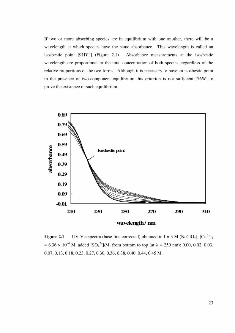
If two or more absorbing species are in equilibrium with one another, there will be a
wavelength at which species have the same absorbance. This wavelength is called an
isosbestic point [91DU] (Figure 2.1). Absorbance measurements at the isosbestic
wavelength are proportional to the total concentration of both species, regardless of the
relative proportions of the two forms. Although it is necessary to have an isosbestic point
in the presence of two-component equilibrium this criterion is not sufficient [76W] to
prove the existence of such equilibrium.
-0.01
0.09
0.19
0.29
0.39
0.49
0.59
0.69
0.79
0.89
210 230 250 270 290 310
wavelength / nm
abso
rbance
.
Isosbestic point
Figure 2.1 UV-Vis spectra (base-line corrected) obtained in I = 3 M (NaClO4), [Cu
2+]T
= 6.36 × 10⁻⁴
M, added [SO42–
]/M, from bottom to top (at λ = 250 nm): 0.00, 0.02, 0.03,
0.07, 0.13, 0.18, 0.23, 0.27, 0.30, 0.36, 0.38, 0.40, 0.44, 0.45 M.
24
2.2 SOLUTION PREPARATION
2.2.1 Reagents
All reagents were prepared using calibrated ‘A’ grade volumetric glassware [88WAB].
Prior to use, the glassware was cleaned with chromic acid and stored with distilled water
[89JBM]. High purity water (Millipore, Milli-Q system) was used in all solution
preparation after boiling for about 30 minutes under high purity nitrogen (Air Liquide) to
minimize dissolved carbonate and oxygen.
Sodium perchlorate was selected as the supporting electrolyte throughout because of its
limited tendency to complex with metal ions and its optical transparency down to ~ 200
nm [70B]. Stock solutions of NaClO4 were prepared by dissolving NaClO4·H2O (99%
BDH AnalaR, pH = 4.5 – 7.0) and filtering through a supported membrane filter (USA,
Versapor-450, 0.45 µm). Such solutions were analysed gravimetrically (± 0.1%) by
dehydration prior to the solution preparation. This process was carried out by sub-boiling
evaporation (80 oC) of triplicate weighed samples of the solution followed by dehydration
at 200 oC to constant weight.
Stock solutions of Na2SO4 were prepared without further purification from the dried
anhydrous salt (99% UNIVAR) and diluted further into various components for preparing
all the other working solutions. A stock solution (~ 0.1 M) of perchloric acid was prepared
by diluting concentrated HClO4 (69-72% w/w, density = 1.70 g/mL, Ajax Chemicals;
Australia) with water (~ 7.2 g to 500 mL). This stock solution was standardized (± 0.2%)
by titration against standard 0.1000 M (± 0.2%) NaOH solution (BDH, Convol, UK), using
methyl orange indicator [89JBM].
A stock solution of Cu(ClO4)2 was prepared by reacting excess CuO (99+% Aldrich, -ACS
reagent) with HClO4 solution The solution was warmed for smooth reaction and filtered
(Millipore 0.45 µm) and a small amount of HClO4 was added to the filtrate to adjust the
pH to 4.5 (using a calibrated glass electrode). The exact concentration of Cu2+
was
determined to ± 0.2% (relative) by titration with standard 0.01000 M EDTA (BDH, UK,
25
concentrated volumetric standard) in solutions buffered with ammonia, with fast sulphon
black F (purple to dark green) as the end point indicator [89JBM].
2.2.2 Difficulties and precautions during solution preparation
All the solutions were made using the same stock solutions, except at the highest ionic
strength where the NaClO4 stock was prepared separately. It was found that when stock
solutions of NaClO4 were mixed either with Na2SO4 or Na2SO4/Cu(ClO4)2 mixtures, a fine
crystalline precipitate appeared. Initially it was thought that this crystallization was caused
by impurities in the NaClO4 stock solution. However, different stock solutions produced
similar results. It was accordingly concluded that the crystallization was due to the
common ion effect lowering the solubility of Na2SO4 at higher NaClO4 concentrations.
Since a low level of copper ions (10–4
or 10–5
M) was used in these experiments, working
solutions were prepared and used the same day to minimize metal ion adsorption on the
glassware. No evidence was observed for significant adsorption of chromophoric species
within the experimental timeframe.
2.3 INSTRUMENTATION AND PROCEDURE
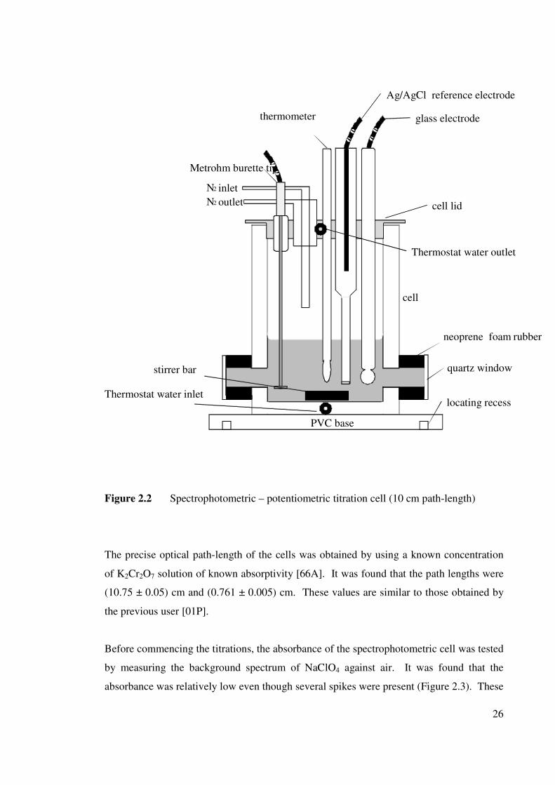
2.3.1 Titration cell
Spectrophotometric titrations were performed in specially-made borosilicate glass cells
(Figure 2.2) that are similar to conventional tall-form water-jacketed potentiometric
titration cells [89JBM]. The present cells contain optically flat quartz windows attached to
the cells via appropriate graded-glass seals to produce nominal optical path-lengths of
either 10 cm or 1 cm. The protruding windows in the 10 cm path-length cell were
insulated using neoprene foam rubber and protected with a stainless steel shield. The
vessels were fitted with snug PTFE [90F] lids machined to provide five standard taper
joints to accommodate the electrodes, N2 gas tubing (in and out), the burette tip and a
thermometer. A fixed mounting made it easy to achieve a reproducible cell alignment in
the spectrophotometer [01P].
26
Figure 2.2 Spectrophotometric – potentiometric titration cell (10 cm path-length)
The precise optical path-length of the cells was obtained by using a known concentration
of K2Cr2O7 solution of known absorptivity [66A]. It was found that the path lengths were
(10.75 ± 0.05) cm and (0.761 ± 0.005) cm. These values are similar to those obtained by
the previous user [01P].
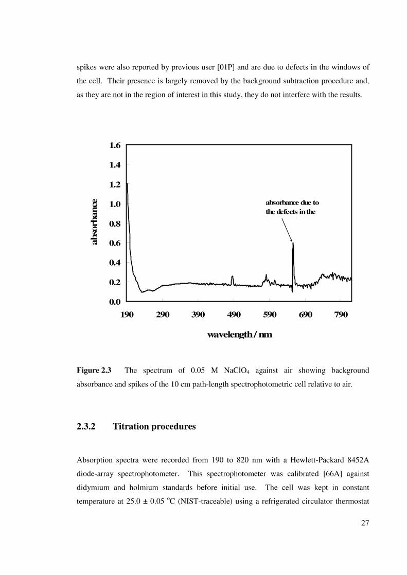
Before commencing the titrations, the absorbance of the spectrophotometric cell was tested
by measuring the background spectrum of NaClO4 against air. It was found that the
absorbance was relatively low even though several spikes were present (Figure 2.3). These
N 2 inlet
N 2 outlet
Metrohm burette tip
thermometer
PVC base
locating recess
quartz window
neoprene foam rubber
Thermostat water inlet
Ag/AgCl reference electrode
glass electrode
Thermostat water outlet
cell lid
stirrer bar
cell
27
spikes were also reported by previous user [01P] and are due to defects in the windows of
the cell. Their presence is largely removed by the background subtraction procedure and,
as they are not in the region of interest in this study, they do not interfere with the results.
0.0
0.2
0.4
0.6
0.8
1.0
1.2
1.4
1.6
190 290 390 490 590 690 790
wavelength / nm
abso
rbance
.
absorbance due to
the defects in the
windows of the
Figure 2.3 The spectrum of 0.05 M NaClO4 against air showing background
absorbance and spikes of the 10 cm path-length spectrophotometric cell relative to air.
2.3.2 Titration procedures
Absorption spectra were recorded from 190 to 820 nm with a Hewlett-Packard 8452A
diode-array spectrophotometer. This spectrophotometer was calibrated [66A] against
didymium and holmium standards before initial use. The cell was kept in constant
temperature at 25.0 ± 0.05 oC (NIST-traceable) using a refrigerated circulator thermostat
28
system (Grant Instruments, UK, type SB3/74GB). As the control unit was somewhat
remote from the spectrophotometer the temperature of the titration solutions was
monitored throughout using a mercury thermometer calibrated against a NIST-traceable
quartz crystal thermometer (Hewlett Packard, 2804, USA). The integration time for all the
measurements was set for 1 second. The cell solutions were stirred throughout with a
PTFE-coated magnetic bar driven by a magnetic rotor (Metrohm, type E402) mounted at
90 o to the cell [01P] to avoid obstruction of the light beam by the stirrer.
During the titration, hydrogen ion concentrations were monitored with a glass electrode
(Metrohm, model 6.0101.000) and a home-made Ag/AgCl reference electrode, used in
conjunction with a salt bridge containing 5.0 M NaClO4. Prior to each titration, the glass
electrode was calibrated using a one point ex-situ measurement of a solution containing
0.01000 M HClO4 in NaClO4 at the appropriate ionic strength. A high impedance digital
voltmeter of in-house construction was used for the potential measurements (± 0.1 mV).
Occasionally, strong acid-strong base titrations were used to check the electrodes for
Nernstian behaviour. It was found that the difference between an ex situ calibration and an
in situ one-point calibration in the presence of Cu2+
was insignificant because of the low
Cu2+
concentration.
2.3.3 Titration method
The titrations were carried out in two different steps: as blank titrations (solutions without
Cu2+
) and complexation titrations (solutions with Cu2+
) at the desired constant ionic
strength of NaClO4. The UV-Vis cell was cleaned and flushed with high purity nitrogen.
Then a known volume (50 mL) of either NaClO4 (for blank titrations) or
Cu(ClO4)2/NaClO4 (for complexation titrations) of the required ionic strength was added to
the titration cell and the electrodes and thermometer fitted.
The cell was connected to the water circulating system and then mounted into the UV-Vis
spectrophotometer. The solution was stirred and N2 used to blanket it. The system was
left to equilibrate for 10 to 15 minutes. When the temperature and potential became stable,
the absorption spectrum was recorded. Then, the burette tip was inserted into the solution
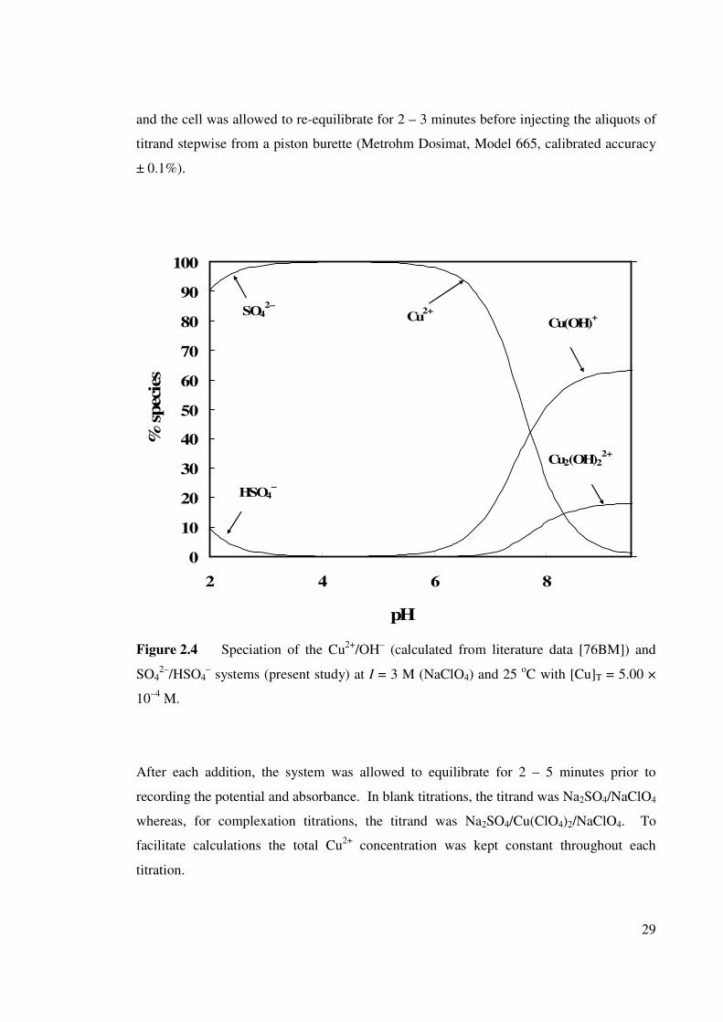
29
and the cell was allowed to re-equilibrate for 2 – 3 minutes before injecting the aliquots of
titrand stepwise from a piston burette (Metrohm Dosimat, Model 665, calibrated accuracy
± 0.1%).
0
10
20
30
40
50
60
70
80
90
100
2 4 6 8
pH
% s
pec
ies
.
Cu(OH)+Cu
2+
Cu2(OH)22+
SO42–
HSO4–
Figure 2.4 Speciation of the Cu2+
/OH– (calculated from literature data [76BM]) and
SO42–
/HSO4– systems (present study) at I = 3 M (NaClO4) and 25
oC with [Cu]T = 5.00 ×
10–4
M.
After each addition, the system was allowed to equilibrate for 2 – 5 minutes prior to
recording the potential and absorbance. In blank titrations, the titrand was Na2SO4/NaClO4
whereas, for complexation titrations, the titrand was Na2SO4/Cu(ClO4)2/NaClO4. To
facilitate calculations the total Cu2+
concentration was kept constant throughout each
titration.
30
All measurements were made between pH 4.0 – 4.5. At this pH the hydrolysis of the
copper ion (Equilibrium 1.23) and also the formation of the bisulfate (HSO4–) ion
(Equilibrium 1.24) are negligible (Figure 2.4). The spectra of the solutions with and
without metal ions were recorded at identical pH values as far as possible to minimize
errors during data processing. Duplicate experiments were performed at each ionic
strength and metal ion concentration.
2.4 DATA ANALYSIS
The data analysis was carried out in several steps. In the first step, the spectra from the
blank titrations at the desired pH values were subtracted from the spectra of the relevant
metal ion-containing solutions by linear interpolation using an EXCEL spreadsheet. The
second step was to select the wavelength range where the background absorbance did not
change by more than 0.1 in the 1 cm cell. A portion of the non-absorbing range was also
included to help in the convergence of the fitting calculation [01P]. Furthermore, the
errors from detector saturation were minimized by ensuring that both the absorbances of
the background and the metal ion solution did not exceed 1.0. It was shown [91DU] with
UV-Visible instruments, the smallest relative error occurs at 0.85 ≤ A ≤ 1. Detector dark
current errors (the current that flows in a photo-detector when there is no optical radiation
incident upon it under normal operating voltages) were removed in step three using a
suitable baseline standardization of the spectra. Subsequently the spectra were evaluated
using the computer program SPECFIT [85GMM(1-3), 86GMM, 98BZ].
2.5 THE SPECFIT PROGRAM
The SPECFIT program [98BZ] is based on a global least-squares fitting of equilibrium and
kinetic systems using factor analysis and Marquardt minimization. Analysis of the present
data was carried out using the M/L/H+ complexation model for a two component system
with model parameter Nc =2. In this system, complexes are normally designated as
(MLH) for a system having metal ions (M), ligand (L) and protons (H). Furthermore, the
free metal ion is given the designation (100) and its stability constant value fixed to unity.
31
The free deprotonated ligand is designated (010) and its known protonation constant value
is included in the model as a fixed parameter. The third character in these designations is
to distinguish species with different states of protonation (eg. 011, 012) [98BZ]. The
unknown parameters are those for the complexed species that are found by various fitting
models.
In this way, the SPECFIT program was used to fit the data to assigned models and to
evaluate the stability constants. In determining these constants, the SPECFIT program
calculated the expected spectrum for each metal complex. Well matched (observed versus
calculated) spectra are an indication of a good fit of the data to the selected model. Factor
analysis was applied to calculate the eigenvalues to account for the variation of the
experimental spectra from the calculated spectra [86GMM]. Evolving factor analysis was
used for estimating concentration profile and component spectra [98BZ]. The model was
selected initially using a dummy stability constant value and then choosing the stability
constant value with the minimum absorbance objective function, the lowest standard
deviations and the lowest overall standard deviation in the absorbances (σabs). The
‘internal’ standard deviation, that is, the standard deviation in the stability constant
calculated by the SPECFIT programme, reflects the goodness-of-fit of the data by the
model [85GMM1]. Further details of the SPECFIT program and its usage are described
elsewhere [85GMM(1-3), 86GMM, 98BZ, 01P].
2.6 RESULTS AND DISCUSSION
2.6.1 Association constants by UV-Vis spectrophotometry
When a Cu(ClO4)2/NaClO4 solution (in the cell) was titrated with Na2SO4/Cu(ClO4)2/
NaClO4 (in the burette) at constant ionic strength, changes occurred in the UV/Vis
absorption spectra in the form of the emergence of a broad shoulder at 230 ≤ λ/nm ≤ 260.
This absorbance increased with increasing total sodium sulfate concentration [Na2SO4]T.
This is illustrated in Figure 2.5, which also includes a spectrum of a solution containing
Cu(ClO4)2 and no Na2SO4 (bottom trace).
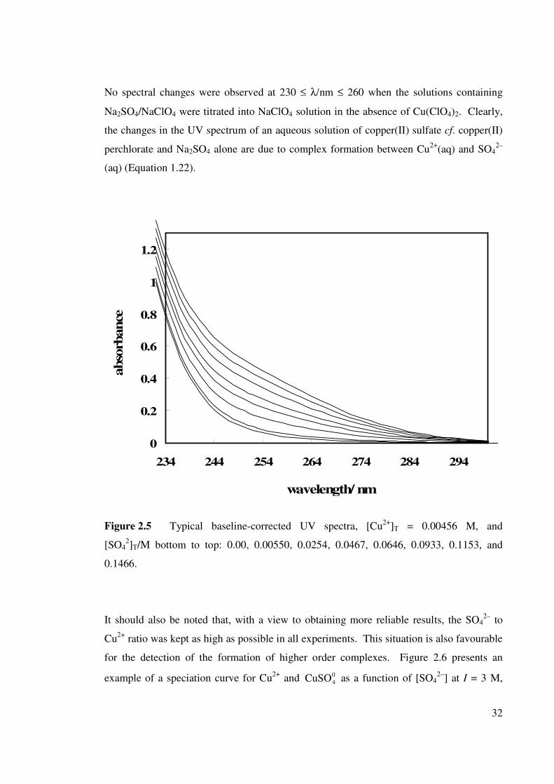
32
No spectral changes were observed at 230 ≤ λ/nm ≤ 260 when the solutions containing
Na2SO4/NaClO4 were titrated into NaClO4 solution in the absence of Cu(ClO4)2. Clearly,
the changes in the UV spectrum of an aqueous solution of copper(II) sulfate cf. copper(II)
perchlorate and Na2SO4 alone are due to complex formation between Cu2+
(aq) and SO42–
(aq) (Equation 1.22).
0
0.2
0.4
0.6
0.8
1
1.2
234 244 254 264 274 284 294
wavelength/ nm
abso
rbance
.
Figure 2.5 Typical baseline-corrected UV spectra, [Cu2+
]T = 0.00456 M, and
[SO42]T/M bottom to top: 0.00, 0.00550, 0.0254, 0.0467, 0.0646, 0.0933, 0.1153, and
0.1466.
It should also be noted that, with a view to obtaining more reliable results, the SO42–
to
Cu2+
ratio was kept as high as possible in all experiments. This situation is also favourable
for the detection of the formation of higher order complexes. Figure 2.6 presents an
example of a speciation curve for Cu2+
and 0
4CuSO as a function of [SO42–
] at I = 3 M,
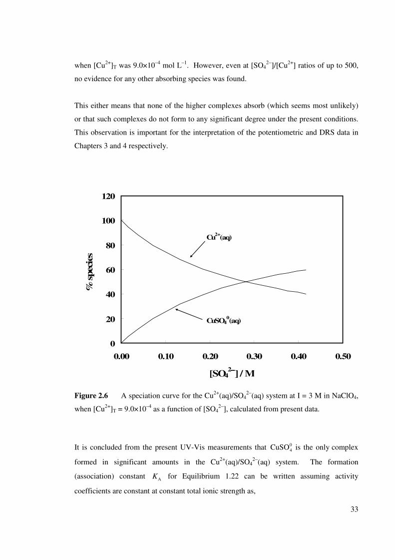
33
when [Cu2+
]T was 9.0×10⁻⁴
mol L–1
. However, even at [SO42–
]/[Cu2+
] ratios of up to 500,
no evidence for any other absorbing species was found.
This either means that none of the higher complexes absorb (which seems most unlikely)
or that such complexes do not form to any significant degree under the present conditions.
This observation is important for the interpretation of the potentiometric and DRS data in
Chapters 3 and 4 respectively.
0
20
40
60
80
100
120
0.00 0.10 0.20 0.30 0.40 0.50
[SO42−−−−
] / M
% s
pec
ies
.
CuSO40(aq)
Cu2+
(aq)
Figure 2.6 A speciation curve for the Cu2+
(aq)/SO42–
(aq) system at I = 3 M in NaClO4,
when [Cu2+
]T = 9.0×10⁻⁴
as a function of [SO42–
], calculated from present data.
It is concluded from the present UV-Vis measurements that 0
4CuSO is the only
complex
formed in significant amounts in the Cu2+
(aq)/SO42–
(aq) system. The formation
(association) constant AK for Equilibrium 1.22 can be written assuming activity
coefficients are constant at constant total ionic strength as,
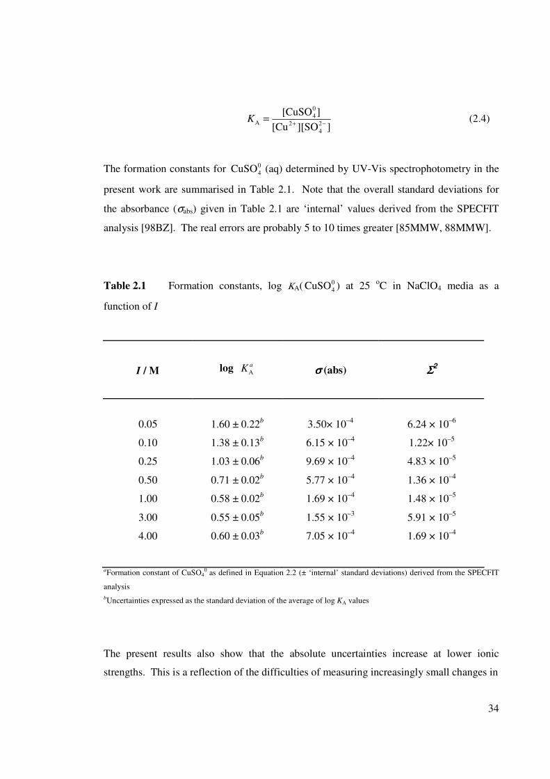
34
]][SO[Cu
][CuSO
2
4
2
0
4A −+
=K (2.4)
The formation constants for 0
4CuSO (aq) determined by UV-Vis spectrophotometry in the
present work are summarised in Table 2.1. Note that the overall standard deviations for
the absorbance (σabs) given in Table 2.1 are ‘internal’ values derived from the SPECFIT
analysis [98BZ]. The real errors are probably 5 to 10 times greater [85MMW, 88MMW].
Table 2.1 Formation constants, log ΚA( 0
4CuSO ) at 25 oC in NaClO4 media as a
function of I
I / M log a
KA σ σ σ σ (abs) ΣΣΣΣ
2
0.05 1.60 ± 0.22b 3.50× 10
–4 6.24 × 10
–6
0.10 1.38 ± 0.13b 6.15 × 10
–4 1.22× 10
–5
0.25 1.03 ± 0.06b 9.69 × 10
–4 4.83 × 10
–5
0.50 0.71 ± 0.02b 5.77 × 10
–4 1.36 × 10
–4
1.00 0.58 ± 0.02b 1.69 × 10
–4 1.48 × 10
–5
3.00 0.55 ± 0.05b 1.55 × 10
–3 5.91 × 10
–5
4.00
0.60 ± 0.03b
7.05 × 10⁻⁴
1.69 × 10⁻⁴
aFormation constant of CuSO40
as defined in Equation 2.2 (± ‘internal’ standard deviations) derived from the SPECFIT
analysis
bUncertainties expressed as the standard deviation of the average of log KA values
The present results also show that the absolute uncertainties increase at lower ionic
strengths. This is a reflection of the difficulties of measuring increasingly small changes in
35
absorbance [79LMZ]. Concentrations of absorbing species at lower ionic strengths are
smaller than those at higher ionic strengths, which increase the uncertainty.
The present results obtained in NaClO4 media for log )(CuSO0
4AK are plotted along with
selected literature data (Table 1.1) in Figure 2.7. The solid curve corresponds to the
extended Guggenheim-type equation
23
1
||2loglog DHo
AA DICIIB
IzzAKK ++
+−= −+ (2.5)
where the adjustable parameters B, C and D have the values of 0.73711, 0.74436 and
– 0.17843 consecutively.
2.6.2 Comparison with literature data
It can be seen (Table 1.1) that spectrophotometry has been a popular method for studying
the formation constant KA )(CuSO0
4 at finite ionic strengths. However, most of these data
were obtained many years ago when spectrophotometer technology was not as advanced
and processing methods were not as sophisticated as they are today. Typically, older data
were obtained using just one or two wavelengths, compared with the present study where
the absorption data were analyzed at wavelengths from 190 ≤ λ/nm ≤ 820. In addition the
titration method used in this study yields spectra at smoothly increasing [SO42–
] under
carefully monitored pH values.
Figure 2.7 shows that the present values are in reasonable agreement with various earlier
studies. However, it is interesting to note that the present results show only a small
increase in the formation constant as a function of ionic strength in the range
1.0 ≤ I/M ≤ 4.0, which is in agreement with the findings of Ashurst and Hancock [77AH].
In contrast, the values of Liu and Yang [85LY] increase significantly at high I. It should
be noted that the smoothness and number of values ascribed to Liu and Yang (Figure 2.7)
is artefactual because they were calculated from their fitting equation
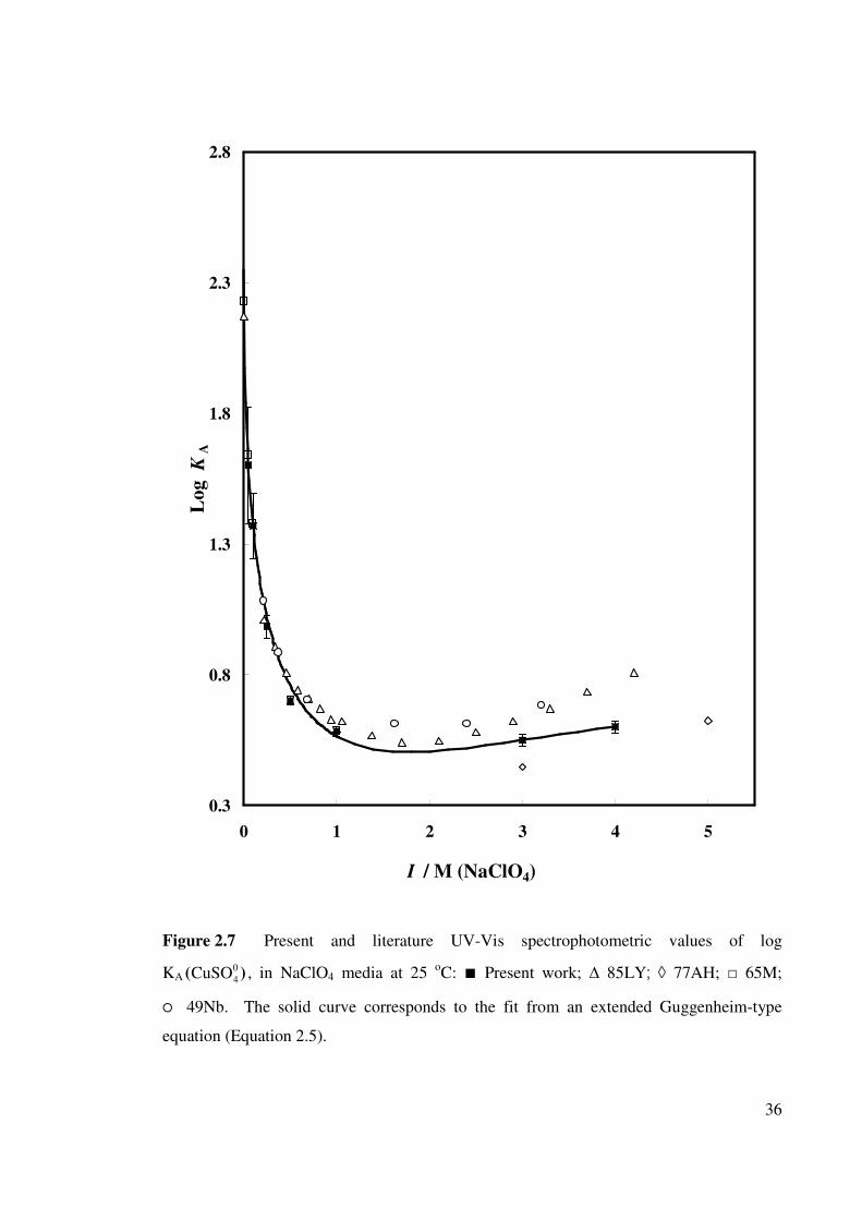
36
0.3
0.8
1.3
1.8
2.3
2.8
0 1 2 3 4 5
I / M (NaClO4)
Lo
g K
A
Figure 2.7 Present and literature UV-Vis spectrophotometric values of log
KA )( 0
4CuSO , in NaClO4 media at 25 oC: Present work; ∆ 85LY; ◊ 77AH; 65M;
49Nb. The solid curve corresponds to the fit from an extended Guggenheim-type
equation (Equation 2.5).
37
2.6.3 Standard state association constant
As can be seen from Table 1.1, most of the earlier reported association constants for
0
4CuSO were determined in dilute solutions, yielding the infinite dilution (standard state)
value o
Alog K . Although not the main focus of the present study, it is worthwhile to
estimate o
AK to compare it with previous work (Table 1.1). For ease of computation an
extended Guggenheim-type equation (Equation 2.5) was selected in this study to obtain the
o
Alog K value of 2.35 ± 0.03 with the other parameters having the values stated above.
2.6.4 Possible occurrence of a second complex
Matheson [65M] studied the possibility of having a second complex −2
24)(CuSO using two
sets of solutions, one with a [SO42–
]/[Cu2+
] ratio of 7 and the other with a [SO42–
]/[Cu2+
]
ratio of ~ 0.14. However, the small difference (≈ 2%) observed by Matheson between the
two solutions, regarded as being due to −2
24)(CuSO , was little greater than the experimental
error. In the present study, the possibility of a second complex was studied by
investigating the [SO42–
]/[Cu2+
] ratios much higher than those of Matheson.
Analysis of the present spectra using the SPECFIT program gave no reason to believe that
there was a second complex in the system over the concentration range studied. Thus, it
seems likely that Matheson’s observation was due either to activity coefficient changes or
to small systematic experimental errors.
Nasanen’s [53N] conclusion on the Cu2+
(aq)/SO42–
(aq) system supports this view. After
studying several combinations of Cu(ClO4)2 and Li2SO4 solutions with total concentration
of 1.0 M, Nasanen found only one complex with similar absorption characteristics to those
of the present study.
38
Chapter Three
Potentiometry
3.1 INTRODUCTION
Potentiometry is a widely applicable, convenient, and accurate technique for the
measurement of metal-complex equilibrium constants [61RR, 88MM]. Although
potentiometry has been a preferred technique for thermodynamic measurements for a
century, its application to the study of chemical equilibria has been revolutionalized
over the last 30 or so years by the development of ion-selective electrodes (ISEs) [75K,
84H]. These electrodes, based on membrane potentials, have considerably augmented
the rather limited range of traditional (redox-based) electrodes that were available
previously. ISEs are also easier to use than traditional electrodes, more robust, usually
subject to less interference, and generally have considerably lower limits of detection.
In a typical potentiometric experiment, the potential developed in a galvanic cell
containing an indicator or working electrode, which responds in some clearly defined
way to solution composition, and a reference electrode whose potential is (ideally)
independent of the solution composition, is measured at near zero current [92SLL].
The overall observable cell potential, Eobs, is therefore, ideally, composed of a constant
potential from the reference electrode and a variable potential that reflects changes in
the activity of the species (ion) of interest [82Ha].
Potentiometric studies can be carried out using cells with or without liquid junctions.
Although, the latter are probably more accurate, they are far less flexible with respect to
the type of equilibria that can be studied because of possible chemical interferences
with the reference electrode. Furthermore, the formation constants obtained from cells
without liquid junction are rather sensitive to the activity coefficient model adopted
[06MH]. Hence, modern potentiometric studies have been mostly carried out in cells
with liquid junction. It is also current practice to perform measurements in solutions
with a ‘constant ionic medium’ in which a large excess of a supposedly non-reactive
background electrolyte, is added in an attempt to maintain constant activity

39
coefficients. The disadvantage of this method is that the equilibrium constants so
obtained are concentration quotients, valid only at the ionic strength in the medium in
which they are measured. The standard state (infinite dilution) equilibrium constant, if
required, must be obtained either by extrapolation to zero of data measured as a
function of ionic strength, I, or by calculation using an appropriate activity coefficient
expression.
In general, for cells with liquid junction the observable potential is given by
Eobs = Eind–Eref + Ej (3.1)
where Eind, Eref and Ej are respectively the potentials of the indicator and reference
electrodes and of any liquid junctions that might be present.
The small but significant liquid junction potentials (LJPs) that exist at interfaces
between electrolyte solutions [82He] represent a fundamental limitation on the
accuracy of direct potentiometric measurements. Such potential differences can be kept
reasonably constant by a suitable interface (cell) construction. Consequently, the most
wide-spread technique for dealing with LJPs is simply to assume them to be negligible.
Hefter [82He] and others [70RS, 78R] have shown that this assumption is frequently
untrue and potentiometric measurements that use this approach may contain
unsuspected but significant systematic errors. Such LJPs can in principle be calculated
using suitable equations such as the Henderson or Planck equations provided certain
conditions are met. However, in this study the approach adopted was to minimise LJPs
(strictly speaking, changes in LJPs) by careful cell design. Accordingly, Equation 3.1
can be written as,
Eobs = Eind - E′ref (3.2)
where Ej = constant, and is incorporated into E′ref.
40
The mathematical relationship between the observable potential of a cell containing an
ISE responsive to the activity of the ion x in solution is described by the Nernst
equation
xobs log303.2
azF
RTEE
−′= (3.3)
where E′ is a constant which includes the rest potential of the indicator electrode, the
potential of the reference electrode and the liquid junction potential [84S], all of which
are assumed to be constant. Of the other terms in Equation 3.3, R is the gas constant
(8.3145 J mol–1
K–1
), T is the temperature in Kelvin, z is the ionic charge number
including its sign and F is the Faraday constant (9.6485 × 10⁴ C mol
–1). The quantity
zF
RT303.2 is called the Nernst factor or theoretical electrode slope and is equal to
59.157/z mV at 25 oC. Equation 3.3 assumes electrode responds only to x and that
there are no other ions in solution to which the indicator electrode responds.
The accuracy of potentiometric measurements employing ISEs depends on the
selectivity of the ISE and the concentration of any interfering ions relative to that of the
ion being measured. This is because the net response of an ISE is described by the
Nikolsky–Eisenman equation [00UBU],
))(log(303.2
yx
X
/
y
y
y,xobs
zz
akazF
RTEE ∑+
−′= (3.4)
where zx, zy and ax, ay are charge numbers and activities of the primary ion, x, and
interfering ion, y respectively; kx,y is the selectivity coefficient for the primary ion x,
against the interfering ion, y. The selectivity coefficient is a measure of the sensitivity
of the electrode to interfering species. It was assumed in this study that there were no
interfering ions at concentrations sufficiently high to cause a significant electrode
response. The reproducibility of EMF measurements using modern ISEs is typically of
the order of ± 0.1 mV, which means that the precision in the determination of
concentration cannot be better than ± 0.4% [78FF].
41
3.2 EXPERIMENTAL STRATEGY
The Cu2+
(aq)/SO42–
(aq) system has been studied using various techniques, mostly by
UV-Vis spectrophotometry, and there is a considerable amount of data available
(Table 1.1). However, as noted in Chapter 1, the reported equilibrium constants show a
significant uncertainty and the thermodynamics of complex formation in the
Cu2+
(aq)/SO42–
(aq) system are not as well characterized as they might be. Surprisingly,
few studies for the Cu2+
/SO42-
system have been made using potentiometry (Table 1.1).
Given the uncertainty about exactly what is detected (in terms of solvent-separated and
contact species) by UV-Vis spectrophotometry it seems worthwhile to undertake a
through study of this system by potentiometry. After reviewing the available data, it
was decided to study the Cu2+
/SO42-
system as a function of ionic strength using
Cu2+
-ISE potentiometry to compare with the results obtained from the UV-Vis studies
(Chapter 2).
3.3 EXPERIMENTAL
3.3.1 Reagents and glassware
Analytical reagent (AR) grade chemicals and calibrated ‘A’-grade volumetric
glassware were used throughout. Prior to use, the glassware was cleaned (Section
2.2.1) and stored filled with distilled water [89JBM]. High purity water (Millipore
Milli Q system) was used for all solution preparation. All such water was boiled for
about 30 minutes under high purity nitrogen (Air Liquide, high purity, Western
Australia) to minimize dissolved carbon dioxide and oxygen.
All the stock solutions of NaClO4, Na2SO4 and Cu(ClO4)2 were prepared according to
the methods described in Section 2.2. These solutions were used to prepare working
solutions by accurate volumetric dilutions. The stoichiometric ionic strength of all
solutions was adjusted by addition of appropriate amounts of NaClO4.
42
3.3.2 Electrodes
A commercial copper(II) ion-selective electrode, (Metrohm, Switzerland, model
6.0502.140) was used throughout. It is a solid state (crystal) membrane ISE with a
claimed measuring range of [Cu2+
] from 10–8
to 10–1
M when used in direct
potentiometry [06A]. The electrode was stored dry between titrations. Before its first
use, and after every few experiments, the electrode surface was reconditioned using a
Metrohm 6.2802.00 polishing set. All potentials were measured relative to a home-
made Ag/AgCl reference electrode consisting of a silver wire in contact with solid
AgCl [72H]. The reference electrode filling solution was 4.9 M NaClO4/0.1 M NaCl
throughout. The reference electrode was separated from the test solution using a salt
bridge containing 5.0 M NaClO4 solution. In this way it is possible to reduce the
diffusion of silver-containing species into the test solution as well as to minimise
variations in the liquid junction potential [82He].
The electrochemical cells used in this work can be represented (ignoring the sign
convention) as
Reference Half Cell Salt Bridge Test Solution
Ag|AgCl|0.1 M NaCl, 4.9 M NaClO4||5.0 M NaClO4||Cu(ClO4) 2,Na2SO4,I(NaClO4)|Cu2+
-ISE
Ej1 Ej2
where Ej1 and Ej2 are liquid junction potentials and I(NaClO4) indicates that the
solution was maintained at constant I by the addition of appropriate amounts of
NaClO4.
3.3.3 Titration apparatus
The cell used for potentiometric titrations (Figure 3.1) was a conventional 100 mL tall-
form glass-jacketed potentiometric titration cell [89JBM]. This cell was fitted with a
snug PTFE lid machined to have five standard taper joints to accommodate the
Cu2+
-ISE, the reference electrode, N2 gas tubing (in and out), and the burette tip. The
temperature of the cell was maintained at 25.0 ± 0.01 oC using a Haake N3 circulator-
thermostat cooled with a secondary refrigerated Neslab circulator-thermostat set to
43
22.0 ± 0.5 oC [03T]. The cell temperature was monitored regularly using a mercury
thermometer calibrated against a NIST-traceable quartz crystal thermometer (Hewlett
Packard, Model HP2804A, USA). Before initiating a titration, as well as during the
titration, atmospheric gases in the titration cell solutions were excluded by the passage
of high purity nitrogen by means of a ‘Springham’ 3-way glass high vacuum tap [99C].
The cell solution was stirred throughout with a PTFE-coated magnetic bar driven by a
magnetic stirrer mounted underneath the cell.
Potentiometric titrations were performed using a Metrohm syringe burette model 665
operated by a computer (IBM XT PC) running the computer program ‘TITRATE’
[90C, 91MMH]. Cell potentials were monitored to ± 0.1 mV by a high impedance
digital voltmeter of in-house construction. During the potentiometric titration, the
‘TITRATE’ computer program collected and recorded the titrant delivery volume and
the cell potentials.
3.3.4 Titration procedure
The potentiometric titrations were carried out in several steps. Initially the pH of all
stock solutions was adjusted to be in the range of 4.0 – 4.5 by adding a small amount of
HClO4. As discussed in Chapter 2, it is assumed that interferences from HSO4– as well
as the hydrolysis products of Cu2+
(aq) are negligible at these pH values. These stock
solutions were diluted to prepare titrant (Na2SO4/NaClO4) and titrand
(Cu(ClO4)2/NaClO4) solutions of the required ionic strength by adding NaClO4
solution. The cell was cleaned and flushed with high purity N2 for 10 minutes to ensure
unwanted O2 and CO2 were removed from the cell atmosphere. A known volume
(usually 15 mL) of Cu(ClO4)2/NaClO4 solution was pipetted into the titration cell and
the electrodes fitted. The solution was stirred with N2 bubbled through it while the
system was left to equilibrate for 10 to 15 minutes. Special care was taken to adjust the
speed of the stirrer and bubbling to avoid N2 bubbles sticking to the Cu2+
-ISE
membrane. The N2 was humidified by passing it through a pre-saturator containing
NaClO4 solution at the same ionic strength as that in the cell.
The next step was to calibrate the electrode pair. This was achieved by an in situ
method, where a dummy titration (one-point calibration) was performed with same
titration set up prior to each titration. A stable potential (to ± 0.1 mV) was usually
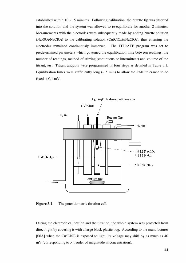
44
established within 10 - 15 minutes. Following calibration, the burette tip was inserted
into the solution and the system was allowed to re-equilibrate for another 2 minutes.
Measurements with the electrodes were subsequently made by adding burette solution
(Na2SO4/NaClO4) to the calibrating solution (Cu(ClO4)2/NaClO4), thus ensuring the
electrodes remained continuously immersed. The TITRATE program was set to
predetermined parameters which governed the equilibration time between readings, the
number of readings, method of stirring (continuous or intermittent) and volume of the
titrant, etc. Titrant aliquots were programmed in four steps as detailed in Table 3.1.
Equilibration times were sufficiently long (∼ 5 min) to allow the EMF tolerance to be
fixed at 0.1 mV.
Figure 3.1 The potentiometric titration cell.
During the electrode calibration and the titration, the whole system was protected from
direct light by covering it with a large black plastic bag. According to the manufacturer
[06A] when the Cu2+
-ISE is exposed to light, its voltage may shift by as much as 40
mV (corresponding to > 1 order of magnitude in concentration).
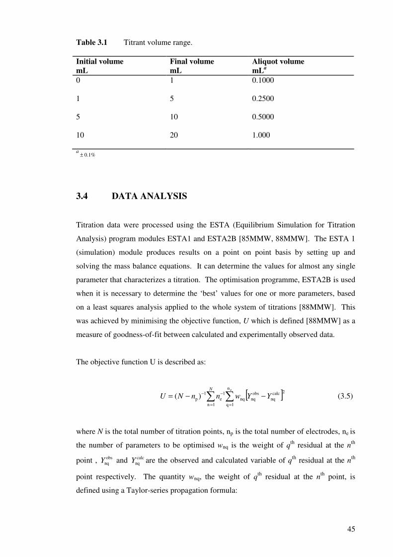
45
Table 3.1 Titrant volume range.
Initial volume
mL
Final volume
mL
Aliquot volume
mLa
0 1 0.1000
1 5 0.2500
5 10 0.5000
10 20 1.000
a ± 0.1%
3.4 DATA ANALYSIS
Titration data were processed using the ESTA (Equilibrium Simulation for Titration
Analysis) program modules ESTA1 and ESTA2B [85MMW, 88MMW]. The ESTA 1
(simulation) module produces results on a point on point basis by setting up and
solving the mass balance equations. It can determine the values for almost any single
parameter that characterizes a titration. The optimisation programme, ESTA2B is used
when it is necessary to determine the ‘best’ values for one or more parameters, based
on a least squares analysis applied to the whole system of titrations [88MMW]. This
was achieved by minimising the objective function, U which is defined [88MMW] as a
measure of goodness-of-fit between calculated and experimentally observed data.
The objective function U is described as:
[ ]2calc
nq
obs
nq
n
1q
nq
1n
1
e
1
p
e
)( YYwnnNU
N
−−= ∑∑==
−− (3.5)
where N is the total number of titration points, np is the total number of electrodes, ne is
the number of parameters to be optimised wnq is the weight of qth
residual at the nth
point , obs
nqY and calc
nqY are the observed and calculated variable of qth
residual at the nth
point respectively. The quantity wnq, the weight of qth
residual at the nth
point, is
defined using a Taylor-series propagation formula:
46
1
p
2
p
2calc
nq
obs
nq
nq
)(−
−= ∑ σ
δ
δ
p
YYw (3.6)
where p represents the parameter optimized and σp is the standard deviation of the
titration parameters held constant during the optimisation [88MMW].
The quality of the calculated equilibrium constant can be obtained by comparing the
independently and simultaneously optimised values. The following qualities are
considered [88MMW] as criteria for a reliable titration and an acceptable equilibrium
constant:
a) low objective function;
b) an equilibrium constant with a small standard deviation;
c) good agreement between the analytical concentrations and the optimised values;
and
d) reproducibility of better than 0.01 log K units between titrations
Titration results not fitting these criteria were rejected.
The number of parameters optimised during the ESTA analysis were minimised so as
to minimise the possible correlations between the parameters being determined. Good
agreement between observed and calculated results gives confidence in the equilibrium
constants obtained from the ESTA analysis [88MMW].
3.5 CHARACTERISATION OF THE BEHAVIOUR OF THE
Cu2+
-ISE
Although Cu2+
-ISEs have been available for some time, they have not been widely used
for the determination of equilibrium constants [90K]. The behaviour of the Cu2+
-ISE is
a critical determinant of the accuracy of the data obtained. Thus it was considered
important to investigate its performance in the NaClO4 media of interest here. In
particular, it was necessary to establish the concentration range over which the
electrode behaved in a Nernstian manner. This was studied by titrating a solution of
47
accurately known concentration of Cu(ClO4)2 in NaClO4 media into a cell containing a
known volume of NaClO4 at the desired ionic strength. Activity coefficients and LJPs
were assumed constant throughout the titration (see Section 3.1) and were incorporated
in to the formal cell potential E ′′ . The observed cell potential Eobs can then be
calculated from the modified Nernst equation (cf. Equation 3.3),
Eobs = E ′′ + k log [Cu2+
] (3.7)
A plot of measured potential versus log [Cu2+
] should therefore give a straight line with
slope of k and an intercept of E ′′ . The constant k is the electrode response slope which
is ideally 29.58 mV at 25 oC.
For several titrations, at relatively higher [Cu2+
], slopes of the plots of Eobs vs. log
[Cu2+
] were found to be sub-Nernstian (Figure 3.2). Unusually for most ion-selective
electrodes, the Cu2+
-ISE showed a tendency (Figure 3.2) towards a sub-Nernstain
response at higher [Cu2+
] (≥ 0.04 M), rather than the much more common deterioration
in the slope found at low concentration [90K, 97CHM, 98CHM ]. This may be an
activity effect associated with the replacing Na+ by Cu
2+ or some non-ideality in the
operation of the Cu2+
-ISE membrane. Further calibrations were performed using lower
[Cu2+
] that were closer to the desired experimental range, at I = 1.0 and 3.0 M NaClO4.
Figures 3.3 and 3.4 show that the slopes of the plot Eobs vs. –log[Cu2+
] over the
concentration range 10–5 ≤ [Cu
2+] / M ≤ 10
–3 were linear and, within the limits of error,
Nernstian. Accordingly, the Nernstian value of the electrode slope (29.58 mV at 25 oC)
was assumed throughout.
3.6 FORMATION CONSTANT OF CuSO 0
4 BY Cu2+
-ISE
POTENTIOMETRY.
The formation constant KA( 0
4CuSO ) corresponding to Equilibrium 1.22 as defined in
Equation 2.4,
]][SO[Cu
][CuSO2
4
2
0
4A −+
=K
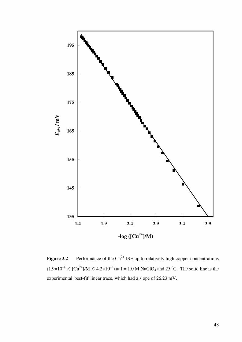
48
135
145
155
165
175
185
195
1.4 1.9 2.4 2.9 3.4 3.9
-log ([Cu2+
]/M)
Eo
bs/
mV
Figure 3.2 Performance of the Cu2+
-ISE up to relatively high copper concentrations
(1.9×10⁻⁴
[Cu2+
]/M 4.2×10⁻²
) at I = 1.0 M NaClO4 and 25 oC. The solid line is the
experimental 'best-fit' linear trace, which had a slope of 26.23 mV.
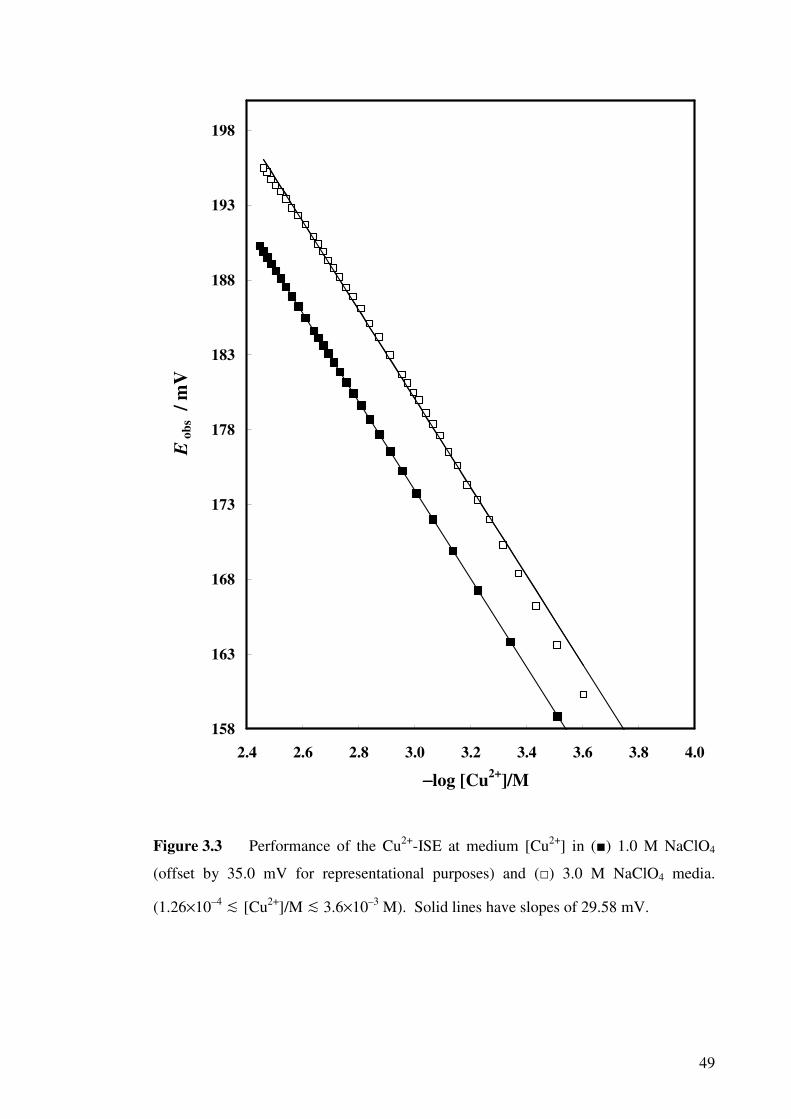
49
158
163
168
173
178
183
188
193
198
2.4 2.6 2.8 3.0 3.2 3.4 3.6 3.8 4.0
−−−−log [Cu2+
]/M
Eo
bs
/ m
V
Figure 3.3 Performance of the Cu2+
-ISE at medium [Cu2+
] in () 1.0 M NaClO4
(offset by 35.0 mV for representational purposes) and () 3.0 M NaClO4 media.
(1.26×10⁻⁴
[Cu2+
]/M 3.6×10⁻³
M). Solid lines have slopes of 29.58 mV.
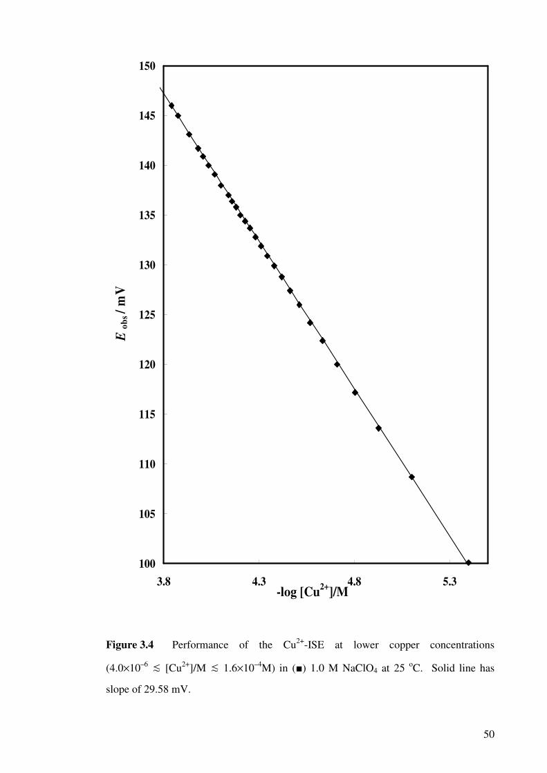
50
100
105
110
115
120
125
130
135
140
145
150
3.8 4.3 4.8 5.3-log [Cu
2+]/M
Eo
bs /
mV
Figure 3.4 Performance of the Cu2+
-ISE at lower copper concentrations
(4.0×10⁻⁶
[Cu2+
]/M 1.6×10⁻⁴
M) in () 1.0 M NaClO4 at 25 oC. Solid line has
slope of 29.58 mV.
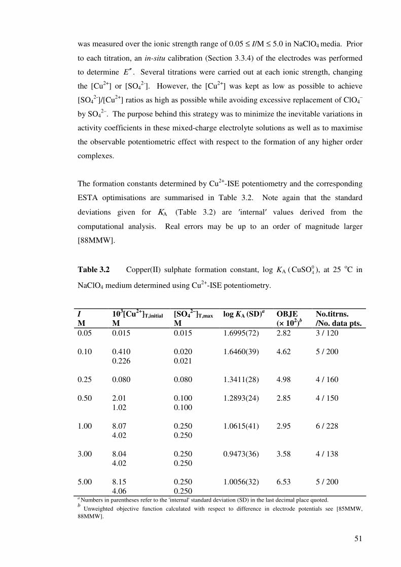
51
was measured over the ionic strength range of 0.05 ≤ I/M ≤ 5.0 in NaClO4 media. Prior
to each titration, an in-situ calibration (Section 3.3.4) of the electrodes was performed
to determine E ′′ . Several titrations were carried out at each ionic strength, changing
the [Cu2+
] or [SO42-
]. However, the [Cu2+
] was kept as low as possible to achieve
[SO42-
]/[Cu2+
] ratios as high as possible while avoiding excessive replacement of ClO4–
by SO42–
. The purpose behind this strategy was to minimize the inevitable variations in
activity coefficients in these mixed-charge electrolyte solutions as well as to maximise
the observable potentiometric effect with respect to the formation of any higher order
complexes.
The formation constants determined by Cu2+
-ISE potentiometry and the corresponding
ESTA optimisations are summarised in Table 3.2. Note again that the standard
deviations given for ΚΑ (Table 3.2) are ′internal′ values derived from the
computational analysis. Real errors may be up to an order of magnitude larger
[88MMW].
Table 3.2 Copper(II) sulphate formation constant, log KA ( 0
4CuSO ), at 25 oC in
NaClO4 medium determined using Cu2+
-ISE potentiometry.
I
M
103[Cu
2+]T,initial
M
[SO42–
]T,max
M
log KA (SD)a OBJE
(× 102)b
No.titrns.
/No. data pts.
0.05 0.015 0.015 1.6995(72) 2.82 3 / 120
0.10 0.410
0.226
0.020
0.021
1.6460(39) 4.62 5 / 200
0.25 0.080 0.080 1.3411(28) 4.98 4 / 160
0.50 2.01
1.02
0.100
0.100
1.2893(24) 2.85 4 / 150
1.00 8.07
4.02
0.250
0.250
1.0615(41) 2.95 6 / 228
3.00 8.04
4.02
0.250
0.250
0.9473(36) 3.58 4 / 138
5.00 8.15
4.06
0.250
0.250
1.0056(32) 6.53 5 / 200
a Numbers in parentheses refer to the 'internal' standard deviation (SD) in the last decimal place quoted. b
Unweighted objective function calculated with respect to difference in electrode potentials see [85MMW,
88MMW].
52
3.7 COMPARISON OF PRESENT RESULTS WITH UV-Vis
RESULTS
The formation constants obtained by potentiometry in NaClO4 media (Table 3.2) are
plotted against I (NaClO4) in Figure 3.5 together with the UV-Vis results from Chapter
2 (Table 2.1). As expected from the activity coefficient expressions (Section 1.4) there
is an initial decrease of log KA followed by an increase with increasing I. As was
apparent in the UV-Vis data there is very little increase in log KA at higher I ( 2 M).
As noted in Chapter 2, UV-Vis results from the present study are comparable with the
literature values obtained using the same method (Figure 2.7). However, as is clear
from Figure 3.5, the UV-Vis determined KA values are significantly lower than the
potentiometric results. Activity coefficient variations cannot explain this difference
since both sets of measurements were carried out in NaClO4 media over similar (albeit
not identical) concentration ranges of Cu2+
and SO42−
. Similarly, any computational or
experimental difficulties experienced for either technique are insufficient to account for
this difference. The most plausible explanation for this difference is that only part of
the association between Cu2+
(aq) and SO42−
(aq) is detected by UV-Vis
spectrophotometry.
As discussed in detail by Hefter [06He] there is strong evidence that many
spectrophotometric techniques including UV-Vis, do not detect all of the ion
association if there are solvent separated ion pairs (2SIP & SIP) present. As will be
shown in Chapter 4, consistent with earlier ultrasonic and dielectric relaxation studies
[65P, 68HP, 70FMH, 92BHB], the existence of such species in aqueous solutions of
copper(II) sulfate is well proven. However these results cannot be unthinkingly applied
to the potentiometry and UV-Visible studies in which Cu2+
and SO42−
interact in the
presence of a large excess of the (assumed) non-interacting NaClO4.
What is actually detected by UV-Vis in the Cu2+
/SO42–
system remains unclear. As
discussed in Section 2.6.1, from its location (λ ≈ 250 nm) and intensity the band
assigned to 0
4CuSO (aq) almost certainly corresponds a L→M charge transfer (LMCT).
Such a transition might well be expected to detect both CIP and SIP species.
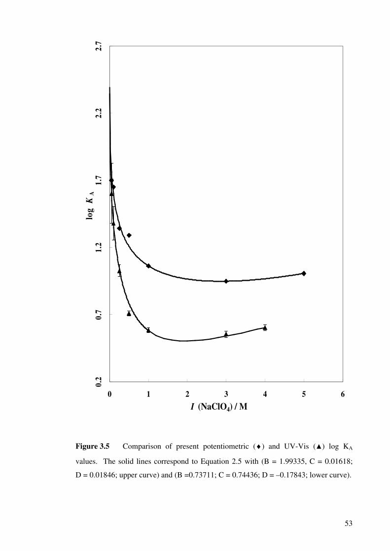
53
0.2
0.7
1.2
1.7
2.2
2.7
0 1 2 3 4 5 6
I (NaClO4) / M
log
K
A
Figure 3.5 Comparison of present potentiometric (♦) and UV-Vis () log KA
values. The solid lines correspond to Equation 2.5 with (B = 1.99335, C = 0.01618;
D = 0.01846; upper curve) and (B =0.73711; C = 0.74436; D = –0.17843; lower curve).
54
However, it would be surprising if a LMCT were able to detect 2SIPs. The failure of
UV-Vis to detect all of the ion pairs present quantitatively accounts for the differences
in Figure 3.5. However, it might be expected that the difference between the
spectrophotometric and potentiometric results would increase at low I, corresponding to
a presumed increase in 2SIP (Figures 4.13 & 4.14). That this does not occur (compare
Tables 2.1 and 3.2) may be a reflection of differences in species (2SIP/SIP/CIP)
distribution between CuSO4(aq) and Cu2+
/SO42–
in NaClO4(aq) media. The increased
uncertainties in the UV-Vis data at low I (Chapter 2) may also contribute to the
difficulties of measuring increasingly small changes in absorbance [79LMZ].
3.8 LITERATURE COMPARISON
Even though, a plethora of values have been obtained for KA ( 0
4CuSO ) using variety of
techniques, no reliable literature data are available in NaClO4 media using Cu2+
-ISE
potentiometry (Table 1.1). The most direct comparison that can be made is with the
value of log KA = 1.17 reported by Fronaeus in 1948 [48F] at I =1.0 (NaClO4) using a
Cu amalgam electrode. This is in good agreement with the present result of log KA =
1.062 (Table 3.2) within the likely true error limits. The lower value of log KA = 0.95
also at I = 1.0 (NaClO4) and 25 oC, later reported by Fronaeus using a quinhydrone
electrode, can be discounted since the reported result is lowered by the claimed
presence of −2
24 )Cu(SO (and even −4
34 )Cu(SO !). As will be discussed below (Section
3.9) the existence of such species are unlikely. The value of log KA = 2.22 at I = 0.1 M
(NaClO4) and 25 oC, also obtained by Cu
2+-ISE potentiometry, is markedly higher than
all other values measured under similar conditions and was rejected in a recent critical
review by IUPAC [07PBB].
3.9 STANDARD STATE ASSOCIATION CONSTANT
Although the focus of this study has been on quantifying the KA )(CuSO0
4 at finite ionic
strengths, it is useful for comparison with literature values to estimate the standard state
value of the formation constant at infinite dilution. As in Chapter 2, the log o
AK value
was obtained from the present log KA(I) results by fitting them to an extended
Guggenheim-type equation (Equation 2.5). The fitting empirical parameters B, C and
D for the Equation 2.5 were found to be 1.9934, 0.01618 and 0.01846 respectively.
55
The value of log o
AK )(CuSO0
4 obtained in this way was 2.39 ± 0.01. This is well
within the stated uncertainty of the value (log o
AK = 2.36 ± 0.07) recommended by
IUPAC from a critical review of all the available data [07PBB]. As would be expected
from the somewhat higher log KA(I) values (Table 3.2) this result is slightly higher, but
has a better precision than, the results obtained from UV-Vis data: log o
AK = 2.35 ±
0.03 (Section 2.6.2). Though the present UV-Vis value is also closer to the value
recommended by IUPAC [07PBB] this is at least in part because those values were
included in the IUPAC evaluation.
3.10 HIGHER-ORDER COMPLEXES
The extensive literature data (Table 1.1) include a number of previous publications
[48F, 51NL, 56K] reporting the existence of higher order complexes, +− )2(1
4 )Cu(SOn
n
(where, n = 2 or 3) [07PBB] using various methods. While all of these studies are
rather old and −4
34 )Cu(SO (aq) can probably be ruled out on charge grounds, the
existence of _2
24 )Cu(SO (aq) remains a possibility, not least because the analogous
species have been detected in other M2+
/SO42–
systems [06AHR, 04BCH].
Accordingly, a detailed potentiometric investigation was undertaken to investigate the
possible formation of _2
24 )Cu(SO (aq) to complement the work reported in Section
2.6.4. To minimise activity coefficient changes, [Cu2+
]T and [SO42–
]T were kept as low
as possible. However, to enhance the possible formation of _2
24 )Cu(SO by employing
very high [SO42–
]T/[Cu2+
]T ratios, significant replacement of ClO4– by SO4
2– was
unavoidable (Table 3.2).
Measurements were made at [SO42–
]T/[Cu2+
]T ratios of up to 1000. The data obtained
were analysed in detail by ESTA using one 0
4(CuSO (aq)) and two 0
4(CuSO (aq) and
_2
24 )Cu(SO (aq)) complex models. The existence (or otherwise) of the second complex
was then assessed using the usual criteria [89MMW]. This included SIME (data
simulation) and ERR% (percentage species distribution) tasks. The results obtained
from these analyses are summarized in Table 3.3.
56
Proof of the existence or non-existence of a minor species by the analysis of
potentiometric titration data alone is not trivial task [88MMW]. May et al. [88MMW]
have suggested the following criteria for this purpose.
• There should be fairly well established formation constant available
in the literature preferably from different techniques.
• Formation constant for species whose percentage formation is
always < 15% are dubious.
• Preference should be given to those species that occur over a wide
range of concentrations and whose percentage formation is rapidly
changing.
The data in Table 3.3 show that the computed second complex, −2
24 )Cu(SO , was lower
than the acceptable value ( 15%) for almost all conditions. At lower I, (0.05 to 0.5
M) where there is a higher [SO42–
]/[Cu2+
] and lower total [SO42–
] than those at higher I
(1.00 to 5.00M), the percentage of [ −2
24 )Cu(SO ] is much below 15%. Table 3.3 also
shows that the effect of apparent formation of a second complex tends to diminish
(11% → 5%) with decreasing [Cu2+
] and [SO42–
].
The only time −2
24 )Cu(SO appears to form to a significant amount is at I = 1.0 M.
However, it may be noted that these titrations also correspond to relatively high [Cu2+
]
and the highest relative replacement level of SO42–
(up to 25%). Furthermore if this
effect were real, a similarly high percentage formation of −2
24 )Cu(SO would be expected
at I = 3 and 5 M (given that the titrations were almost identical sulfate and copper
concentrations). This is clearly not the case (Table 3.3). This suggests that the
apparent significant formation of −2
24 )Cu(SO at I = 1 M (NaClO4) is an artefact.
A number of other factors support the conclusion that −2
24 )Cu(SO does not form to a
significant extent under the present conditions. First, the slightly improved objective
functions obtained for Model 2 are not necessarily significant because an extra
optimising parameter is involved. Furthermore, for some titrations OBJE is actually
worse, or not significantly better, for Model 2 (I = 1.0 M). Second, it can be noted that
the standard deviations in log K1 and log K2 are considerably worse than those obtained
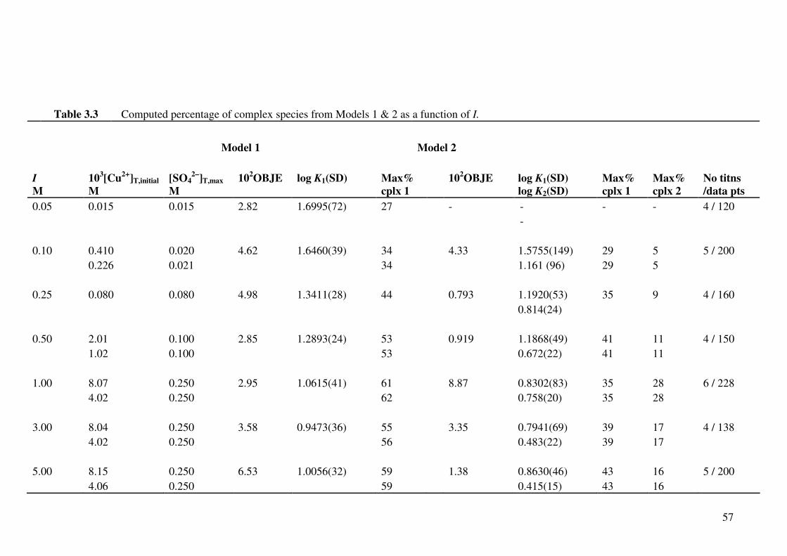
57
Table 3.3 Computed percentage of complex species from Models 1 & 2 as a function of I.
Model 1 Model 2
I
M
103[Cu
2+]T,initial
M
[SO42–
]T,max
M
102OBJE
log K1(SD)
Max%
cplx 1
102OBJE
log K1(SD)
log K2(SD)
Max%
cplx 1
Max%
cplx 2
No titns
/data pts
0.05 0.015 0.015 2.82 1.6995(72) 27 - - - - 4 / 120
-
0.10 0.410 0.020 4.62 1.6460(39) 34 4.33 1.5755(149) 29 5 5 / 200
0.226 0.021 34 1.161 (96) 29 5
0.25 0.080 0.080 4.98 1.3411(28) 44 0.793 1.1920(53) 35 9 4 / 160
0.814(24)
0.50 2.01 0.100 2.85 1.2893(24) 53 0.919 1.1868(49) 41 11 4 / 150
1.02 0.100 53 0.672(22) 41 11
1.00 8.07 0.250 2.95 1.0615(41) 61 8.87 0.8302(83) 35 28 6 / 228
4.02 0.250 62 0.758(20) 35 28
3.00 8.04 0.250 3.58 0.9473(36) 55 3.35 0.7941(69) 39 17 4 / 138
4.02 0.250 56 0.483(22) 39 17
5.00 8.15 0.250 6.53 1.0056(32) 59 1.38 0.8630(46) 43 16 5 / 200
4.06 0.250 59 0.415(15) 43 16
58
for log K1 alone in Model 1. In particular the very large standard deviations for log K2
in Model 2 imply a lack of real significance in the apparent formation of this species.
Third, it was found during the optimisation process (data not shown) that there were
strong correlations in Model 2 between log K2 and other parameters (such as titrant
concentration) that were being held constant.
Finally, apart from the present potentiometric results, there is only one previous report,
by Fronaeus [48F], of higher order complex formation in the Cu2+
/SO42–
system.
However, as discussed in Section 3.8, Fronaeus’ conclusions [48F] are unreliable
because they include the highly improbable −4
34 )Cu(SO species. Neither dielectric
relaxation (Chapter 5) nor Raman spectroscopy studies on Cu2+
/SO42–
system show any
evidence for the formation of −2
24 )Cu(SO . Nor indeed was there any UV-Vis evidence
for its formation even at [SO42–
]/[Cu2+
] ratios of up to 500. On the basis of all the
above points, it is concluded that the evidence for the existence of −2
24 )Cu(SO in the
present solutions is unconvincing. Its apparent formation, in relatively small amounts,
is almost certainly an artefact due to activity coefficient variations as significant
replacement of the swamping medium ions Na+ and ClO4
– by Cu
2+ and/or SO4
2–.
59
Chapter Four
Dielectric Relaxation Spectroscopy
Dielectric relaxation spectroscopy (DRS) measures the complex dielectric response of a
medium as a function of the frequency of an applied alternating electric field, [95C, 94BB]
generally in the microwave region. DRS has been widely used in material sciences to
characterize solids [83Jo], polymers [77H] or meso-phases [83B]. In biophysics and
pharmacy it has been used in the analysis of colloids and suspensions [95C]. More
recently, DRS has become an efficient tool to investigate the structure of electrolyte
solutions [97BB, 98BBE, 98BKK], ion association, solvation and ion-solvent interactions
as well as the dynamics of molecular interactions in liquids and solutions [90BBB, 91BB,
94BHB, 95C, 98BBE, 03BSM].
Selectivity for dipolar species is a key feature of DRS, which makes it possible to detect
double solvent-separated (2SIP), solvent-shared (SIP), and contact (CIP) ion pairs in
equilibrium with ‘free’ ions in solution. As explained in Chapter 3, thermodynamic
methods such as potentiometry provide no information about the presence of distinct types
of ion-pairs having the same ion stoichiometry, although they do provide information
about the overall level of ion pairing. UV-Vis and the other popular forms of spectroscopy
(such NMR and Raman) also provide little information about such species since they
mostly detect only CIPs.
Thus, DRS was selected to further investigate the nature of the Cu2+
(aq)/SO42–
(aq) system.
In particular, DRS offers the possibility of a more detailed look at Equilibrium 1.22 which
has been quantified (Chapters 2 & 3) by the more precise (but less insightful) methods of
UV-Vis spectroscopy and potentiometry.
60
4.1 DIELECTRIC THEORY
Dielectric relaxation refers to the response of a dielectric medium to an applied oscillating
electric field. The relaxation results from the movement of dipoles due to the changing
polarity of the field typically in the frequency range of 102 – 10
10 Hz [98BKK]. In the
absence of the field, because of thermal motion, dipoles present in the system are randomly
oriented. At lower frequencies, when the direction of the applied field changes, the net
orientation of the dipoles also changes but they still oscillate around a mean. At higher
frequencies, the field direction changes rapidly and the dipoles are unable to re-orient with
the field because of their inherent inertia and viscous damping from the surrounding
solvent. As a result the total polarization of the system in the electric field falls. However,
between these two extremes, there is a characteristic frequency, where the re-orientation
process is at maximum and the rate of the change in the direction of the applied field
matches the relaxation time of the dipoles.
This time-dependent electric polarization )(tP
ρ, which describes the effect of an electric
field on the medium, is the sum of the orientational polarization, µP
ρ,
)()( tEPo
ρρ
∞−= εεεµ (4.1)
and the induced polarization, α
P
ρ,
)()1( tEPo
ρρ−=
∞εεα (4.2)
where ∞
ε is the infinite frequency permittivity and
αµ+= PPtP
ρρρ)( (4.3)
Therefore,
)()1()( tEtPo
ρρ−= εε (4.4)
where εo and ε are the permittivity of free space and the relative permittivity of the sample
respectively [78BB] and )(tE
ρ is the strength of the applied electric field.
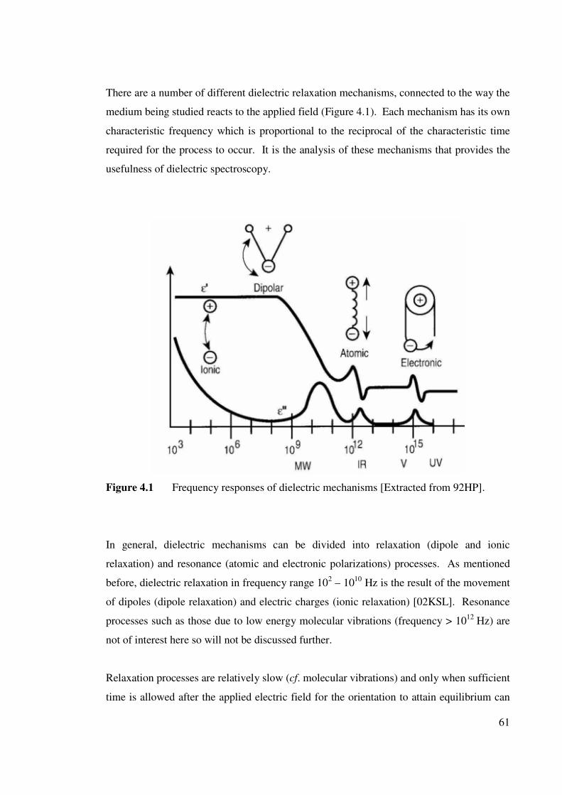
61
There are a number of different dielectric relaxation mechanisms, connected to the way the
medium being studied reacts to the applied field (Figure 4.1). Each mechanism has its own
characteristic frequency which is proportional to the reciprocal of the characteristic time
required for the process to occur. It is the analysis of these mechanisms that provides the
usefulness of dielectric spectroscopy.
Figure 4.1 Frequency responses of dielectric mechanisms [Extracted from 92HP].
In general, dielectric mechanisms can be divided into relaxation (dipole and ionic
relaxation) and resonance (atomic and electronic polarizations) processes. As mentioned
before, dielectric relaxation in frequency range 102 – 1010 Hz is the result of the movement
of dipoles (dipole relaxation) and electric charges (ionic relaxation) [02KSL]. Resonance
processes such as those due to low energy molecular vibrations (frequency > 1012
Hz) are
not of interest here so will not be discussed further.
Relaxation processes are relatively slow (cf. molecular vibrations) and only when sufficient
time is allowed after the applied electric field for the orientation to attain equilibrium can
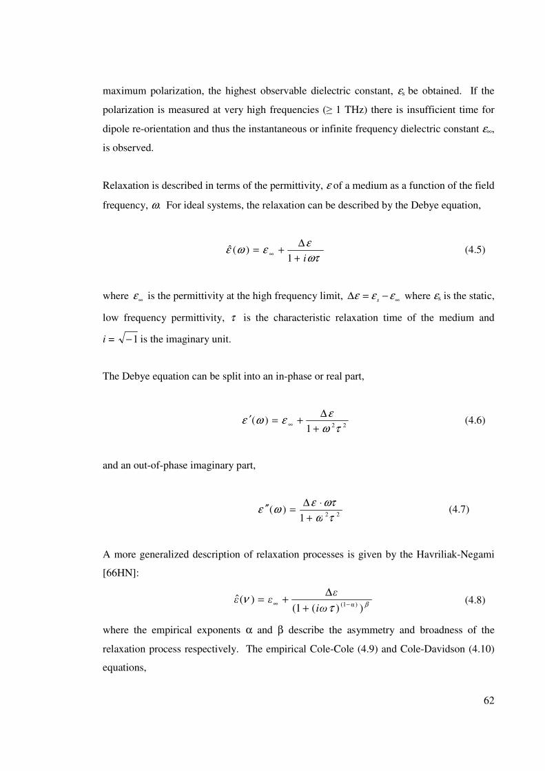
62
maximum polarization, the highest observable dielectric constant, εs be obtained. If the
polarization is measured at very high frequencies (≥ 1 THz) there is insufficient time for
dipole re-orientation and thus the instantaneous or infinite frequency dielectric constant ε∞,
is observed.
Relaxation is described in terms of the permittivity, ε of a medium as a function of the field
frequency, ω. For ideal systems, the relaxation can be described by the Debye equation,
ωτ
εεωε
i+
∆+= ∞
1)(ˆ (4.5)
where ∞
ε is the permittivity at the high frequency limit, ∞
−=∆ εεεs
where εs is the static,
low frequency permittivity, τ is the characteristic relaxation time of the medium and
i = 1− is the imaginary unit.
The Debye equation can be split into an in-phase or real part,
221)(
τω
εεωε
+
∆+=′
∞ (4.6)
and an out-of-phase imaginary part,
221
)(τω
ωτεωε
+
⋅∆=′′ (4.7)
A more generalized description of relaxation processes is given by the Havriliak-Negami
[66HN]:
βτ
ν))(1(
)(ˆ)α1( −∞
+
∆+=
iω
εεε (4.8)
where the empirical exponents α and β describe the asymmetry and broadness of the
relaxation process respectively. The empirical Cole-Cole (4.9) and Cole-Davidson (4.10)
equations,
63
)α1()(1)(ˆ
−∞+
∆+=
τν
iω
εεε (4.9)
βi
εε)(1
)(ˆωτ
εν
+
∆+=
∞ (4.10)
are special cases of the Havriliak-Negami relaxation model corresponding to the peak
shapes when β = 1 (Cole-Cole) and α = 0 (Cole-Davidson). However, the selection of the
correct model to fit all the relaxations depends on the system studied as well as the
frequency range covered. The characteristic relaxation function of the spectrum reflects
the dispersion of )(νε ′ from the zero frequency value (corresponding to the static
permittivity, ε) to infinite frequency, ∞
ε . The corresponding absorption is expressed by
the dielectric loss, )(νε ′′ and the overall complex dielectric response is given by
=)(ˆ νε )(νε ′ – ).(νε ′′i (4.11)
4.2 DRS OF CuSO4(aq) SOLUTIONS
As discussed in detail in Chapters 1 – 3, CuSO4(aq) solutions are appreciably associated at
moderate concentrations, with only one thermodynamically-significant equilibrium
(Equation 1.22). In addition to the techniques discussed previously (Tables 1.1 & 1.2), this
equilibrium has also been studied in particular, using ultrasonic relaxation techniques by
Bechteler et al. [70BBT] and others [68HP, 68Ma, 68PK, 70FHP, 70FMH]. These studies
have established that the three equilibria in Equation 1.19 are present in CuSO4(aq)
solutions. However, because of the then-existing technological restrictions, only limited
information about the various ion pairing equilibria was obtained [04BCH].
On the other hand, previous DRS studies of the Cu2+
(aq)/SO42–
(aq) system appear to be
limited to that of Pottel [65P]. His pioneering study of this system was made at various
temperatures from 5 to 55 oC but at only one concentration (~ 1 mol/L). Although Pottel
was able to identify the presence of 2SIPs and SIPs he could derive only limited
thermodynamic information for them.
64
As DRS can detect the presence of small concentrations of ion pairs and also distinguish
between various types [99BCH], a detailed investigation of CuSO4(aq) using modern
broadband DRS over wide range of concentration and temperature has been undertaken as
part of the present study.
4.3 EXPERIMENTAL
4.3.1 Instrumentation
Dielectric spectra consisting of 101 points at equally spaced increments of log ν over the
frequency range νmin ≤ ν/GHz ≤ 20 were measured at Murdoch University with a Hewlett-
Packard model HP 85070M dielectric probe system, consisting of a HP 8720D vector
network analyzer (VNA; nominal bandwidth 0.05 to 20 GHz) and a HP 85070M dielectric
probe kit (0.2 to 20 GHz stated bandwidth) as described in detail elsewhere [99BCH,
99BHM]. The HP 85070M dielectric software for the VNA was used to control the
instrument and to calculate the dielectric permittivity, ε'(ν), and the total loss η"(ν), from
the experimentally determined relative complex reflection coefficient. The measurable
total loss is related to the desired dielectric loss via:
η"(ν) = ε"(ν) +κ/2πνεo, (4.12)
where κ is the solution conductivity and other symbols have already been defined.
The accuracy of these measurements is estimated to be around 3% for ε'(ν) and 5% for
η"(ν), with a reproducibility 2 – 4 times better [99BHM]. The minimum frequency of the
investigation, νmin, was governed by the conductivity contribution to the loss spectrum. As
such, it varied with solute concentration and temperature but typically was in the range
0.2 – 0.5 GHz.
The temperature of the solutions was controlled with a Hetofrig (Denmark) circular-
thermostat with precision of ± 0.02 oC and an accuracy of about ± 0.05
oC (NIST-
traceable) throughout. Temperature constancy was checked from time to time with a Zeal
65
mercury-in-glass thermometer calibrated against a quartz crystal thermometer (Hewlett
Packard, 2804, USA).
Higher frequency data were determined at Regensburg University by Dr. N. Rohman
[06AHR] using two waveguide interferometers (IFMs): A-band (27 ≤ ν/GHz ≤ 39) and E-
band (60 ≤ ν/GHz ≤ 89) as described in detail elsewhere [91BBB, 98BBE]. Temperatures
were controlled using a Lauda (Germany) model RKS 20 circulator-thermostat with
similar precision and accuracy to those at Murdoch University.
4.3.2 Solution preparation
Copper sulfate pentahydrate samples, CuSO4·5H2O (AR grade, Ajax Chemicals, Australia,
or Merck, Germany) were used as received. The solutions were prepared by weight
without buoyancy corrections using high purity (Millipore Milli-Q) water and A-grade
glassware throughout. Exact metal ion concentrations were determined (as per Chapter 2)
to ± 0.2% by complexometric titration [69SF] against EDTA (BDH, U.K., concentrated
volumetric standard) using fast sulphon black indicator. The density data required for the
conversion from molality (m, mol/kg–solvent) to molarity (c, mol/L–solution) were taken
from the literature [92ZA].
4.3.3 Calibration of the VNA
Before commencing the measurements at the required temperature, the apparatus needed to
be calibrated. A satisfactory calibration partly eliminates spurious signals arising from the
less-than-ideal behaviour of the probe-head and from the cable between the probe-head and
the VNA. All VNA spectra were recorded at least three times using independent
calibrations with air, mercury (as a short circuit) and water as the standards. The
calibration parameters for water at 5, 25, 45 and 65 oC were taken from Buchner et al.
[99BHM].
66
4.4 MEASUREMENT PROCEDURE AND DATA ANALYSIS
Dielectric experiments were performed for aqueous solutions of CuSO4 at concentrations
in the range 0.02 m/mol kg–1 1.4 and temperatures 5 ≤ t/
oC ≤ 65. The minimum
concentration was determined by the sensitivity of the DR spectrometers while the
maximum concentration was governed by the magnitude of the solution conductivity. The
complex permittivity spectra of the solutions were measured in triplicate using independent
calibrations. The calibrations were repeated after a maximum of 5 samples. The complex
permittivity spectra ε (ν) = ε'(ν) – iε"(ν) consisted of the VNA data and (where recorded)
IFM measurements as a function of ν.
The loss component ε"(ν) is not directly observable and must be obtained from the
measurable total loss, as shown in Equation 4.12. As described elsewhere [99BHM],
conductivity corrections to η"(ν) to obtain ε"(ν) were made by treating κ as an adjustable
parameter. Nevertheless, and as found for other solutions, the values of κ so obtained
(Tables 4.1 - 4.4) are in reasonable agreement (Figure 4.2) with the somewhat limited and
scattered bulk solution conductivity data available in the literature [59SA, 73Pi, 80PLD].
Typical dielectric spectra of CuSO4(aq), for representative concentrations, at 5 and 45 oC
are given in Figures 4.3 and 4.4. The effects of temperature are shown more clearly in
Figures 4.5 and 4.6, which present DR spectra at two concentrations over the full
temperature range studied (5 ≤ t/oC ≤ 65). These spectra were analyzed by simultaneously,
fitting the in-phase (relative permittivity, ε'(ν), parts a of Figures 4.3 – 4.6) and out-of-
phase (loss ε"(ν), parts b of Figures 4.3 - 4.6) components to plausible relaxation models
based on the sum of n distinguishable dispersion steps, as described in detail elsewhere
[04BCH].
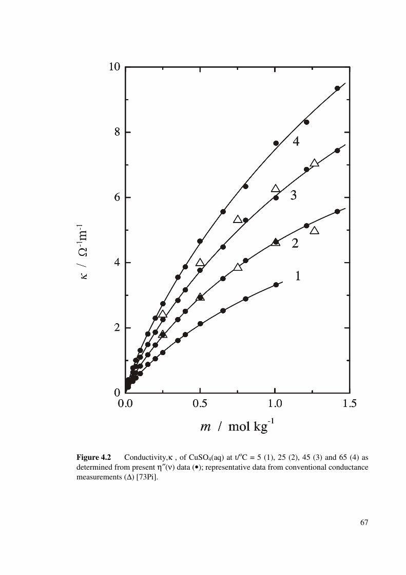
67
Figure 4.2 Conductivity,κ , of CuSO4(aq) at t/oC = 5 (1), 25 (2), 45 (3) and 65 (4) as
determined from present η″(ν) data (•); representative data from conventional conductance
measurements (∆) [73Pi].
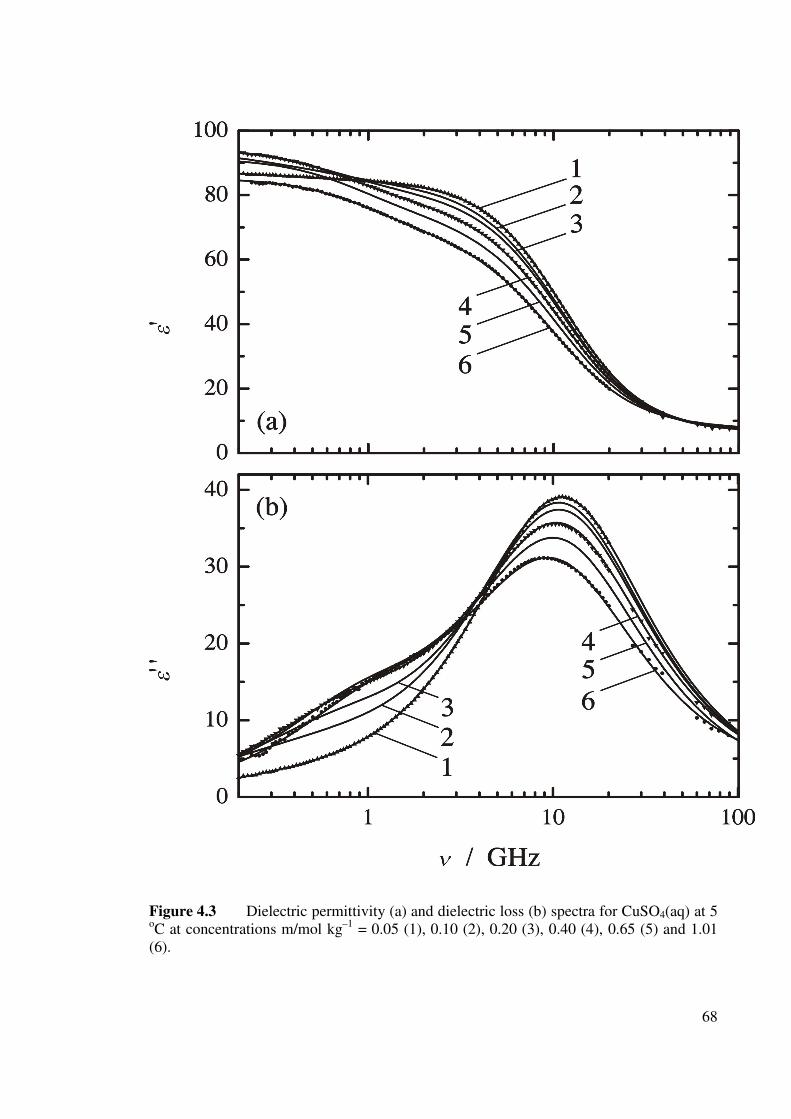
68
Figure 4.3 Dielectric permittivity (a) and dielectric loss (b) spectra for CuSO4(aq) at 5 oC at concentrations m/mol kg
–1 = 0.05 (1), 0.10 (2), 0.20 (3), 0.40 (4), 0.65 (5) and 1.01
(6).
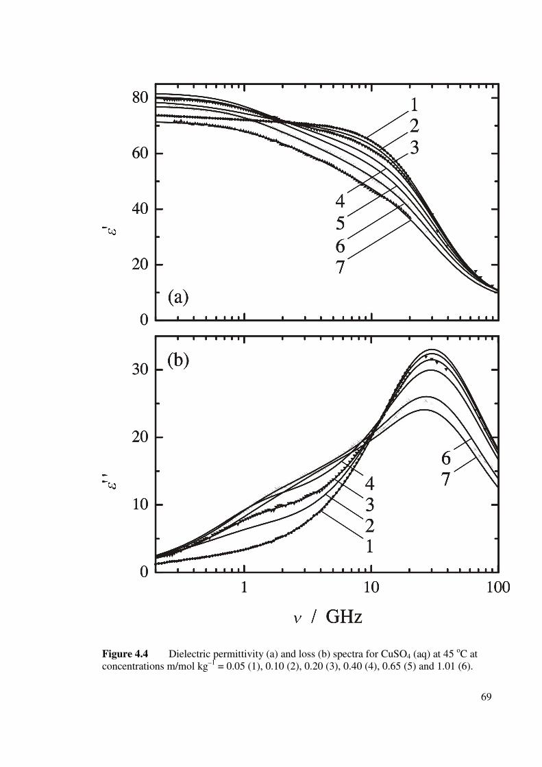
69
Figure 4.4 Dielectric permittivity (a) and loss (b) spectra for CuSO4 (aq) at 45 oC at
concentrations m/mol kg–1
= 0.05 (1), 0.10 (2), 0.20 (3), 0.40 (4), 0.65 (5) and 1.01 (6).
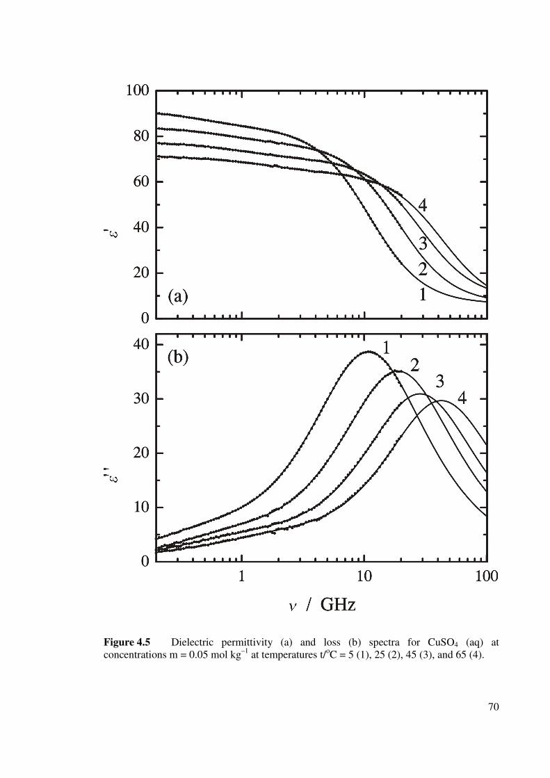
70
Figure 4.5 Dielectric permittivity (a) and loss (b) spectra for CuSO4 (aq) at
concentrations m = 0.05 mol kg–1
at temperatures t/oC = 5 (1), 25 (2), 45 (3), and 65 (4).

71
Figure 4.6 Dielectric permittivity (a) and loss (b) spectra for CuSO4 (aq) at
concentrations m = 0.40 mol kg–1
at temperatures t/oC = 5 (1), 25 (2), 45 (3), and 65 (4).
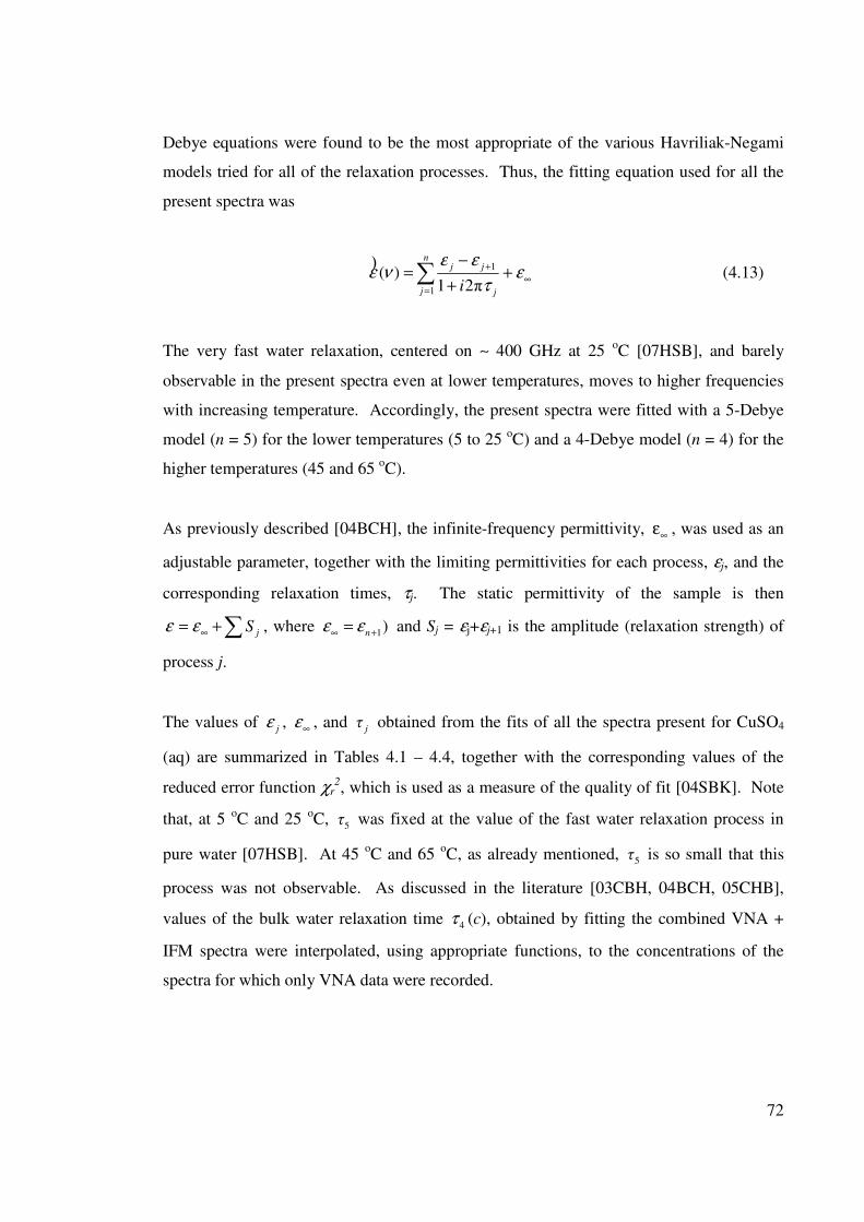
72
Debye equations were found to be the most appropriate of the various Havriliak-Negami
models tried for all of the relaxation processes. Thus, the fitting equation used for all the
present spectra was
∞
=
++
+
−=∑ ε
τ
εενε
n
j j
jj
i1
1
π21)(
) (4.13)
The very fast water relaxation, centered on ∼ 400 GHz at 25 oC [07HSB], and barely
observable in the present spectra even at lower temperatures, moves to higher frequencies
with increasing temperature. Accordingly, the present spectra were fitted with a 5-Debye
model (n = 5) for the lower temperatures (5 to 25 oC) and a 4-Debye model (n = 4) for the
higher temperatures (45 and 65 oC).
As previously described [04BCH], the infinite-frequency permittivity, ∞
ε , was used as an
adjustable parameter, together with the limiting permittivities for each process, εj, and the
corresponding relaxation times, τj. The static permittivity of the sample is then
∑+= ∞ jSεε , where )1+∞
=n
εε and Sj = εj+εj+1 is the amplitude (relaxation strength) of
process j.
The values of j
ε , ∞
ε , and jτ obtained from the fits of all the spectra present for CuSO4
(aq) are summarized in Tables 4.1 – 4.4, together with the corresponding values of the
reduced error function χr
2, which is used as a measure of the quality of fit [04SBK]. Note
that, at 5 oC and 25
oC,
5τ was fixed at the value of the fast water relaxation process in
pure water [07HSB]. At 45 oC and 65
oC, as already mentioned, 5τ is so small that this
process was not observable. As discussed in the literature [03CBH, 04BCH, 05CHB],
values of the bulk water relaxation time 4τ (c), obtained by fitting the combined VNA +
IFM spectra were interpolated, using appropriate functions, to the concentrations of the
spectra for which only VNA data were recorded.
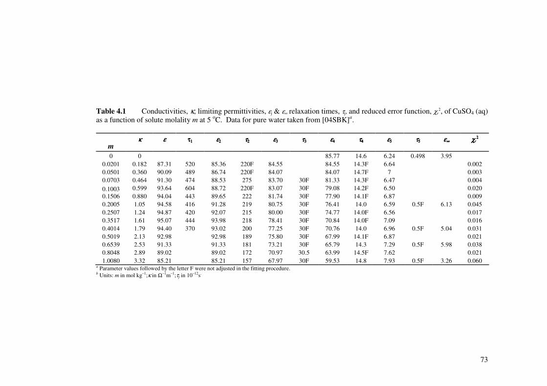
73
Table 4.1 Conductivities, κ, limiting permittivities, εj & ε∞ relaxation times, τj, and reduced error function, χr
2, of CuSO4 (aq)
as a function of solute molality m at 5 oC. Data for pure water taken from [04SBK]
a.
κκκκ εεεε ττττ1111 εεεε2222 ττττ2222 εεεε3333 ττττ3333 εεεε4444 ττττ4444 εεεε5555 ττττ5555 εεεε∞∞∞∞ χχχχr
2222
m
0 0 85.77 14.6 6.24 0.498 3.95
0.0201 0.182 87.31 520 85.36 220F 84.55 84.55 14.3F 6.64 0.002
0.0501 0.360 90.09 489 86.74 220F 84.07 84.07 14.7F 7 0.003
0.0703 0.464 91.30 474 88.53 275 83.70 30F 81.33 14.3F 6.47 0.004
0.599 93.64 604 88.72 220F 83.07 30F 79.08 14.2F 6.50 0.020 0.1003
0.1506 0.880 94.04 443 89.65 222 81.74 30F 77.90 14.1F 6.87 0.009
0.2005 1.05 94.58 416 91.28 219 80.75 30F 76.41 14.0 6.59 0.5F 6.13 0.045
0.2507 1.24 94.87 420 92.07 215 80.00 30F 74.77 14.0F 6.56 0.017
0.3517 1.61 95.07 444 93.98 218 78.41 30F 70.84 14.0F 7.09 0.016
0.4014 1.79 94.40 370 93.02 200 77.25 30F 70.76 14.0 6.96 0.5F 5.04 0.031
0.5019 2.13 92.98 92.98 189 75.80 30F 67.99 14.1F 6.87 0.021
0.6539 2.53 91.33 91.33 181 73.21 30F 65.79 14.3 7.29 0.5F 5.98 0.038
0.8048 2.89 89.02 89.02 172 70.97 30.5 63.99 14.5F 7.62 0.021
1.0080 3.32 85.21 85.21 157 67.97 30F 59.53 14.8 7.93 0.5F 3.26 0.060 a Parameter values followed by the letter F were not adjusted in the fitting procedure. b Units: m in mol kg
–1;κ in Ω
–1m
–1;τj in 10
–12s
.
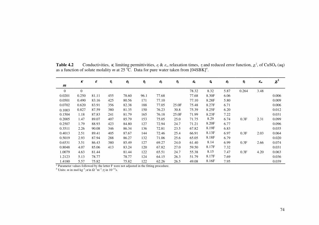
74
Table 4.2 Conductivities, κ, limiting permittivities, εj & ε∞, relaxation times, τj and reduced error function, χr
2, of CuSO4 (aq)
as a function of solute molality m at 25 oC. Data for pure water taken from [04SBK]
a.
κκκκ εεεε ττττ1111 εεεε2222 ττττ2222 εεεε3333 ττττ3333 εεεε4444 ττττ4444 εεεε5555 ττττ5555 εεεε∞∞∞∞ χχχχr
2222
m
0 0 78.32 8.32 5.87 0.264 3.48
0.0201 0.250 81.11 455 78.60 96.1 77.68 77.68 8.30F 6.06 0.006
0.0501 0.490 83.16 425 80.56 171 77.10 77.10 8.28F 5.80 0.009
0.0702 0.620 83.91 356 82.38 188 77.05 25.0F 75.48 8.27F 6.71 0.006
0.827 87.59 380 81.35 150 76.23 30.8 75.39 8.25F 6.20 0.012 0.1003
0.1504 1.18 87.83 241 81.79 165 76.18 25.0F 71.99 8.23F 7.22 0.031
0.2005 1.47 89.07 407 85.79 153 75.05 25.0 71.75 8.29 6.74 0.3F 2.31 0.099
0.2507 1.79 88.93 423 84.80 127 72.94 24.7 71.21 8.20F 6.77 0.096
0.3511 2.26 90.08 346 86.34 136 72.81 23.5 67.82 8.19F 6.83 0.035
0.4013 2.51 89.41 405 87.67 144 72.46 25.4 66.91 8.13F 6.97 0.3F 2.03 0.064
0.5019 2.93 87.94 288 86.27 132 71.06 25.6 65.05 8.18F 6.79 0.020
0.6531 3.51 86.43 380 85.49 127 69.27 24.0 61.40 8.14 6.99 0.3F 2.66 0.074
0.8048 4.07 85.06 413 83.24 120 67.82 27.0 59.50 8.17F 7.32 0.031
1.0079 4.63 81.44 81.44 122 65.51 24.7 55.38 8.15 7.47 0.3F 4.20 0.063
1.2123 5.13 78.77 78.77 124 64.15 26.3 51.79 8.17F 7.69 0.036
1.4180 5.57 75.82 75.82 122 62.26 26.5 49.08 8.16F 7.95 0.039 a Parameter values followed by the letter F were not adjusted in the fitting procedure. b Units: m in mol kg–1;κ in Ω–1m–1;τj in 10–12s.
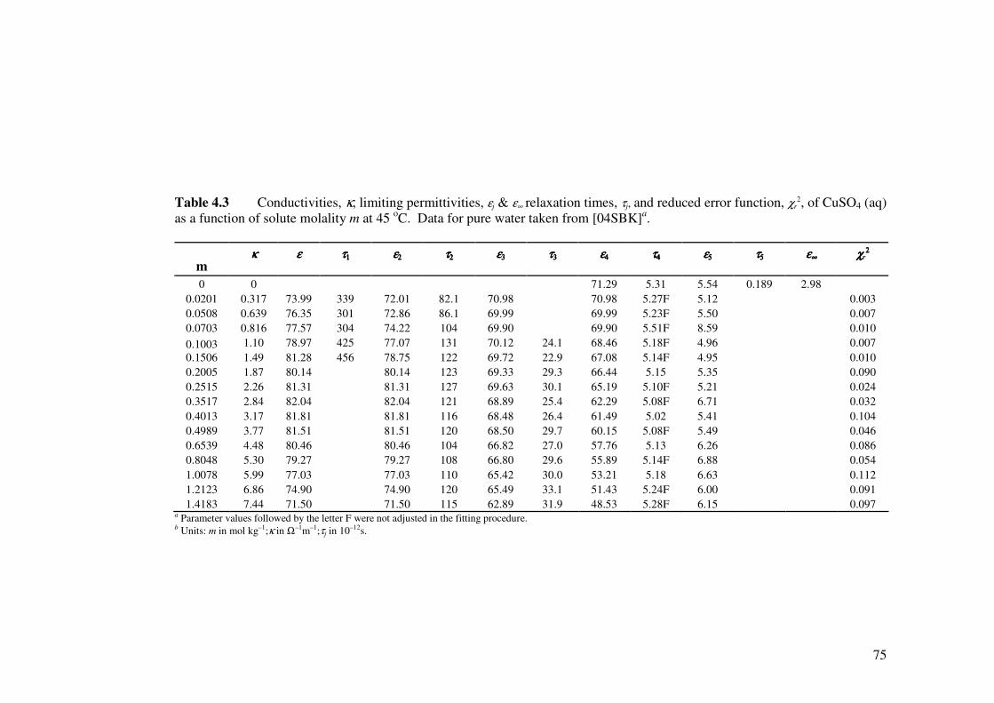
75
Table 4.3 Conductivities, κ, limiting permittivities, εj & ε∞ relaxation times, τj, and reduced error function, χr
2, of CuSO4 (aq)
as a function of solute molality m at 45 oC. Data for pure water taken from [04SBK]
a.
κκκκ εεεε ττττ1111 εεεε2222 ττττ2222 εεεε3333 ττττ3333 εεεε4444 ττττ4444 εεεε5555 ττττ5555 εεεε∞∞∞∞ χχχχr
2222
m
0 0 71.29 5.31 5.54 0.189 2.98
0.0201 0.317 73.99 339 72.01 82.1 70.98 70.98 5.27F 5.12 0.003
0.0508 0.639 76.35 301 72.86 86.1 69.99 69.99 5.23F 5.50 0.007
0.0703 0.816 77.57 304 74.22 104 69.90 69.90 5.51F 8.59 0.010
1.10 78.97 425 77.07 131 70.12 24.1 68.46 5.18F 4.96 0.007 0.1003
0.1506 1.49 81.28 456 78.75 122 69.72 22.9 67.08 5.14F 4.95 0.010
0.2005 1.87 80.14 80.14 123 69.33 29.3 66.44 5.15 5.35 0.090
0.2515 2.26 81.31 81.31 127 69.63 30.1 65.19 5.10F 5.21 0.024
0.3517 2.84 82.04 82.04 121 68.89 25.4 62.29 5.08F 6.71 0.032
0.4013 3.17 81.81 81.81 116 68.48 26.4 61.49 5.02 5.41 0.104
0.4989 3.77 81.51 81.51 120 68.50 29.7 60.15 5.08F 5.49 0.046
0.6539 4.48 80.46 80.46 104 66.82 27.0 57.76 5.13 6.26 0.086
0.8048 5.30 79.27 79.27 108 66.80 29.6 55.89 5.14F 6.88 0.054
1.0078 5.99 77.03 77.03 110 65.42 30.0 53.21 5.18 6.63 0.112
1.2123 6.86 74.90 74.90 120 65.49 33.1 51.43 5.24F 6.00 0.091
1.4183 7.44 71.50 71.50 115 62.89 31.9 48.53 5.28F 6.15 0.097 a Parameter values followed by the letter F were not adjusted in the fitting procedure. b Units: m in mol kg–1;κ in Ω–1m–1;τj in 10–12s.
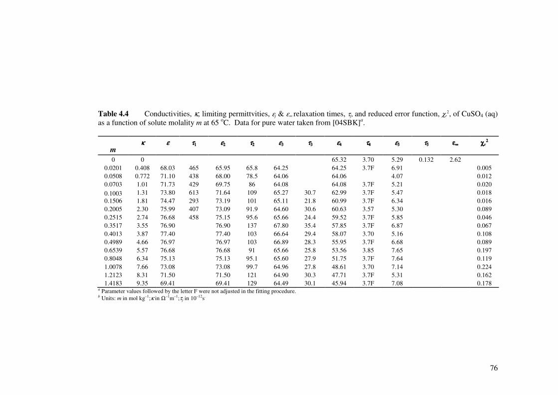
76
Table 4.4 Conductivities, κ, limiting permittvities, εj & ε∞ relaxation times, τj, and reduced error function, χr
2, of CuSO4 (aq)
as a function of solute molality m at 65 oC. Data for pure water taken from [04SBK]
a.
κκκκ εεεε ττττ1111 εεεε2222 ττττ2222 εεεε3333 ττττ3333 εεεε4444 ττττ4444 εεεε5555 ττττ5555 εεεε∞∞∞∞ χχχχr2222
m
0 0 65.32 3.70 5.29 0.132 2.62
0.0201 0.408 68.03 465 65.95 65.8 64.25 64.25 3.7F 6.91 0.005
0.0508 0.772 71.10 438 68.00 78.5 64.06 64.06 4.07 0.012
0.0703 1.01 71.73 429 69.75 86 64.08 64.08 3.7F 5.21 0.020
1.31 73.80 613 71.64 109 65.27 30.7 62.99 3.7F 5.47 0.018 0.1003
0.1506 1.81 74.47 293 73.19 101 65.11 21.8 60.99 3.7F 6.34 0.016
0.2005 2.30 75.99 407 73.09 91.9 64.60 30.6 60.63 3.57 5.30 0.089
0.2515 2.74 76.68 458 75.15 95.6 65.66 24.4 59.52 3.7F 5.85 0.046
0.3517 3.55 76.90 76.90 137 67.80 35.4 57.85 3.7F 6.87 0.067
0.4013 3.87 77.40 77.40 103 66.64 29.4 58.07 3.70 5.16 0.108
0.4989 4.66 76.97 76.97 103 66.89 28.3 55.95 3.7F 6.68 0.089
0.6539 5.57 76.68 76.68 91 65.66 25.8 53.56 3.85 7.65 0.197
0.8048 6.34 75.13 75.13 95.1 65.60 27.9 51.75 3.7F 7.64 0.119
1.0078 7.66 73.08 73.08 99.7 64.96 27.8 48.61 3.70 7.14 0.224
1.2123 8.31 71.50 71.50 121 64.90 30.3 47.71 3.7F 5.31 0.162
1.4183 9.35 69.41 69.41 129 64.49 30.1 45.94 3.7F 7.08 0.178 a Parameter values followed by the letter F were not adjusted in the fitting procedure. b Units: m in mol kg–1;κ in Ω–1m–1;τj in 10–12s.
77
At 5 oC, the CIP relaxation time 3τ (c), had to be fixed at 30 ps to resolve that process
because the dominant and strongly temperature-dependent bulk water relaxation
(4τ ≈ 14 ps) was in general too close to allow separation of process 3 in free-running fits.
On the other hand, the temperature dependence of 4τ facilitated separation of the ion-pair
processes at 45 and 65 oC, which partly compensated for the higher uncertainties at these
temperatures arising from the increased solution conductivity (Figure 4.2).
Typical examples of the decomposition of the observed loss spectra into their component
processes at representative temperatures are given in Figures 4.7 – 4.8. Experimental data
were fitted with the 5D model (Equation 4.12) at 5 oC and the 4D model at 65
oC (see
above).
4.5 RESULTS AND DISCUSSION
4.5.1 General features of ion association
As discussed in Chapter 1, the Cu2+
(aq)/SO42–
(aq) system has been studied extensively
(Table 1.1). It was also noted that the data have been reviewed recently for IUPAC
[07PBB] where it was indicated that these data show a wider-than-expected variation, that
may be due partly to the presence of solvent-separated ion pairs (2SIPs and SIPs). As far
as thermodynamic methods such as potentiometry (Chapter 3) are concerned, the formation
of solvent-separated ion pairs is unimportant because there is no thermodynamic
distinction between dissolved species with the same stoichiometry but having different
degrees of solvation [79HH]. This means thermodynamic methods measure only the
overall association constant, KA, corresponding to Equilibrium 1.22. Similar
considerations apply to conductance data, at least for symmetrical electrolytes where all
ion-pair types are considered to be (equally) nonconducting [83J]. Conductance
measurements therefore produce KA values that are directly comparable with
thermodynamic results. On the other hand, the presence of the various ion-pair types
creates certain difficulties for both the activity coefficient corrections and the conductivity
expressions that are typically used in the analysis of conductance data [83J]. For strong
complexes these problems are not significant.
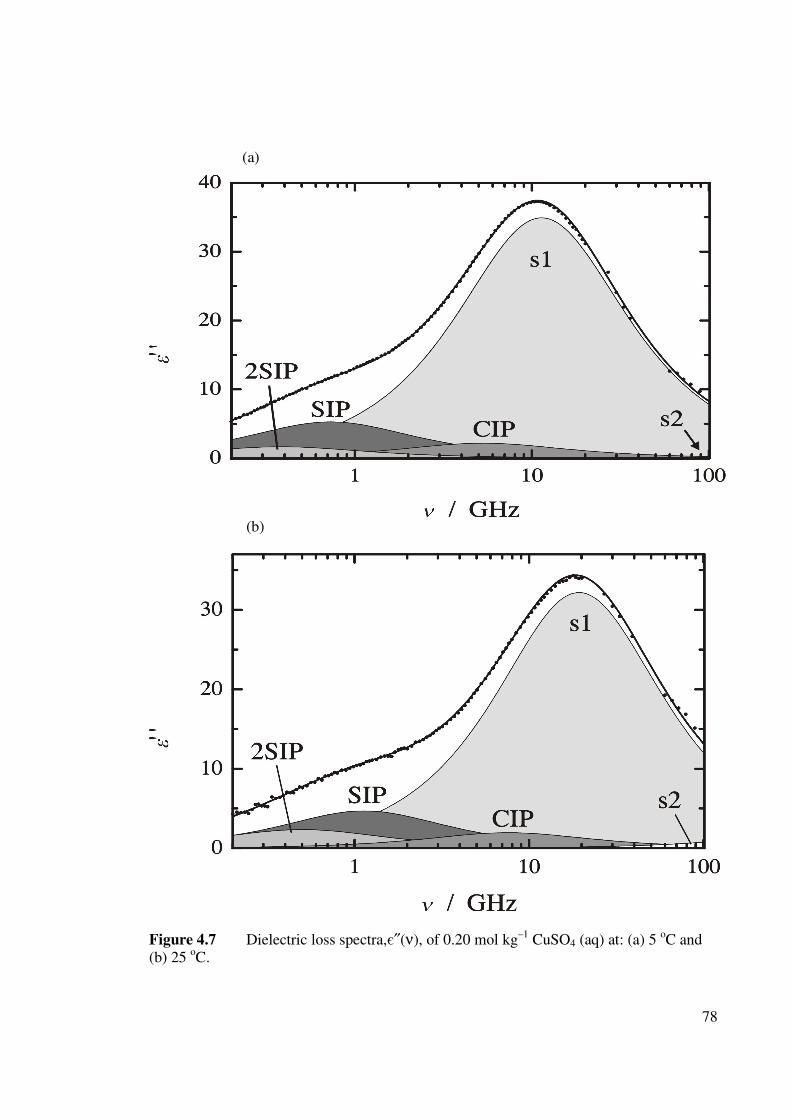
78
(a)
(b)
Figure 4.7 Dielectric loss spectra,є″(ν), of 0.20 mol kg–1
CuSO4 (aq) at: (a) 5 oC and
(b) 25 oC.
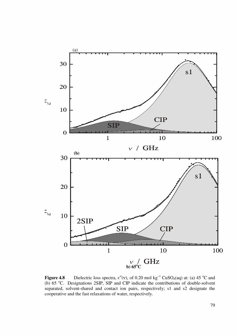
79
(a)
(b)
b) 65
oC
Figure 4.8 Dielectric loss spectra, є″(ν), of 0.20 mol kg–1
CuSO4(aq) at: (a) 45 oC and
(b) 65 oC. Designations 2SIP, SIP and CIP indicate the contributions of double-solvent
separated, solvent-shared and contact ion pairs, respectively; s1 and s2 designate the
cooperative and the fast relaxations of water, respectively.
80
However, for relatively modest association, as occurs in the Cu2+
(aq)/SO42–
(aq) system,
they can become important. These problems have long been recognized and discussed at
length in the literature on many occasions [71HPP, 72P, 05BBP]. Their major effect is to
increase the uncertainty in the calculated values of KA even for the highest quality data.
For spectroscopic measurements, however, the situation is quite different. As discussed in
detail in Chapter 3 and elsewhere [06He], the major spectroscopic methods (NMR, Raman
and UV-Vis) typically detect only CIPs. The association constant determined from such
measurements is thus typically smaller than the values obtained from thermodynamic or
conductance data [57C, 06He]. For example, conventional analysis of high-quality Raman
spectra yields oKA
( 0
4CuSO (aq)) ≈ 10 [08RIH], which is more than an order of magnitude
lower than the values from thermodynamic or conductivity studies [06He]. Furthermore,
although the CIP concentrations determined from Raman spectroscopy [08RIH] are the
same as those obtained by the other techniques (such as DRS) the equilibrium constant is
not directly comparable with either KA or Ki [04BCH].
The present dielectric spectra (see for example, Figures 4.3 & 4.4) indicate the presence of
all three ion-pair types at appropriate conditions of solute concentration and temperature.
Typical decompositions of representative loss spectra are given in Figures 4.7 and 4.8.
The existence of the various ion-pair types is confirmed in DRS (as it is with other
spectroscopic techniques) by the growth and decay of spectral features as functions of
concentration. This is seen more clearly in Figure 4.9, which plots the total solute
contribution to the loss spectra εIP"(ν), as a function of concentration. Also included in
Figure 4.9 are the average peak frequencies of the loss spectrum associated with each ion-
pair species, corresponding to the relaxation times of jτ /ps ≈ 400 (2SIP), 100 (SIP), and
27 (CIP) for j = 1, 2, and 3 respectively.
4.5.2 Analysis of the ion association
The amplitudes S1, S2, and S3 arising from the presence of 2SIPs, SIPs and CIPs
respectively, were analyzed as described previously [04BCH, 05CHB] using the modified
Cavell equation [92BHB]
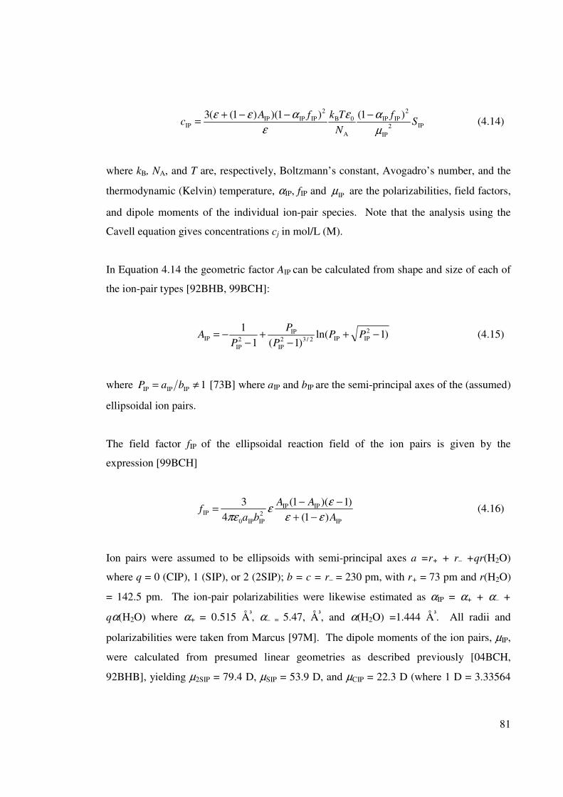
81
IP2
IP
2
IPIP
A
0B
2
IPIPIPIP
)1()1)()1((3S
f
N
TkfAc
µ
αε
ε
αεε −−−+= (4.14)
where kB, NA, and T are, respectively, Boltzmann’s constant, Avogadro’s number, and the
thermodynamic (Kelvin) temperature, αIP, fIP and IPµ are the polarizabilities, field factors,
and dipole moments of the individual ion-pair species. Note that the analysis using the
Cavell equation gives concentrations cj in mol/L (M).
In Equation 4.14 the geometric factor AIP can be calculated from shape and size of each of
the ion-pair types [92BHB, 99BCH]:
)1ln()1(1
1 2
IPIP2/32
IP
IP
2
IP
IP −+−
+−
−= PPP
P
PA (4.15)
where 1IPIPIP ≠= baP [73B] where aIP and bIP are the semi-principal axes of the (assumed)
ellipsoidal ion pairs.
The field factor fIP of the ellipsoidal reaction field of the ion pairs is given by the
expression [99BCH]
IP
IPIP
2
IPIP0
IP)1(
)1)(1(
4
3
A
AA
baf
εε
εε
πε −+
−−= (4.16)
Ion pairs were assumed to be ellipsoids with semi-principal axes a =r+ + r– +qr(H2O)
where q = 0 (CIP), 1 (SIP), or 2 (2SIP); b = c = r– = 230 pm, with r+ = 73 pm and r(H2O)
= 142.5 pm. The ion-pair polarizabilities were likewise estimated as αIP = α+ + α– +
qα(H2O) where α+ = 0.515 ų, α– = 5.47, Å
³, and α(H2O) =1.444 Å
³. All radii and
polarizabilities were taken from Marcus [97M]. The dipole moments of the ion pairs, µIP,
were calculated from presumed linear geometries as described previously [04BCH,
92BHB], yielding µ2SIP = 79.4 D, µSIP = 53.9 D, and µCIP = 22.3 D (where 1 D = 3.33564
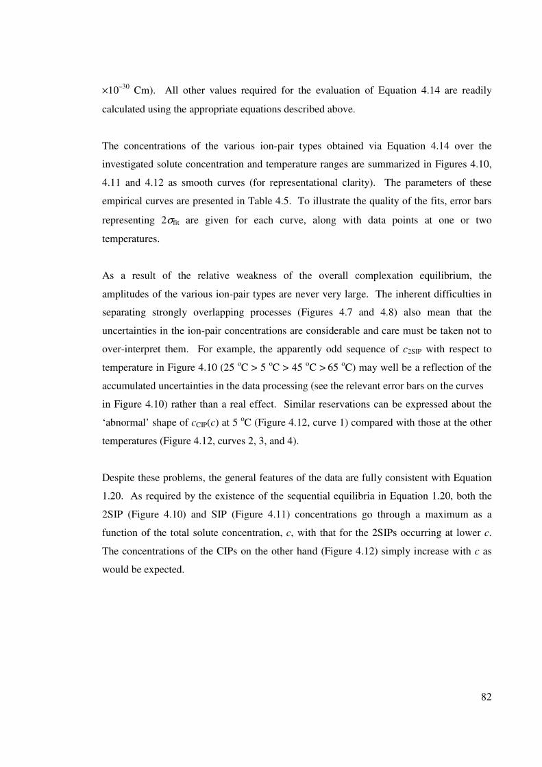
82
×10–30
Cm). All other values required for the evaluation of Equation 4.14 are readily
calculated using the appropriate equations described above.
The concentrations of the various ion-pair types obtained via Equation 4.14 over the
investigated solute concentration and temperature ranges are summarized in Figures 4.10,
4.11 and 4.12 as smooth curves (for representational clarity). The parameters of these
empirical curves are presented in Table 4.5. To illustrate the quality of the fits, error bars
representing 2σfit are given for each curve, along with data points at one or two
temperatures.
As a result of the relative weakness of the overall complexation equilibrium, the
amplitudes of the various ion-pair types are never very large. The inherent difficulties in
separating strongly overlapping processes (Figures 4.7 and 4.8) also mean that the
uncertainties in the ion-pair concentrations are considerable and care must be taken not to
over-interpret them. For example, the apparently odd sequence of c2SIP with respect to
temperature in Figure 4.10 (25 oC > 5
oC > 45
oC >
65
oC) may well be a reflection of the
accumulated uncertainties in the data processing (see the relevant error bars on the curves
in Figure 4.10) rather than a real effect. Similar reservations can be expressed about the
‘abnormal’ shape of cCIP(c) at 5 oC (Figure 4.12, curve 1) compared with those at the other
temperatures (Figure 4.12, curves 2, 3, and 4).
Despite these problems, the general features of the data are fully consistent with Equation
1.20. As required by the existence of the sequential equilibria in Equation 1.20, both the
2SIP (Figure 4.10) and SIP (Figure 4.11) concentrations go through a maximum as a
function of the total solute concentration, c, with that for the 2SIPs occurring at lower c.
The concentrations of the CIPs on the other hand (Figure 4.12) simply increase with c as
would be expected.
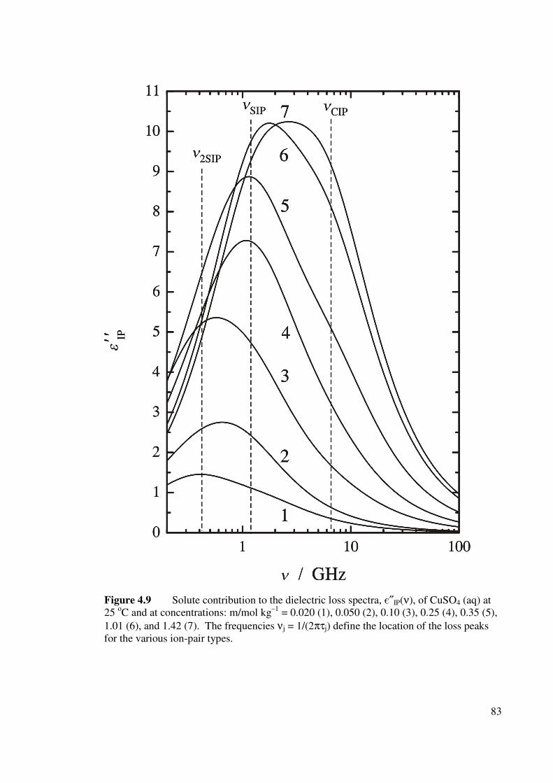
83
Figure 4.9 Solute contribution to the dielectric loss spectra, є″IP(ν), of CuSO4 (aq) at
25 oC and at concentrations: m/mol kg
–1 = 0.020 (1), 0.050 (2), 0.10 (3), 0.25 (4), 0.35 (5),
1.01 (6), and 1.42 (7). The frequencies νj = 1/(2πτj) define the location of the loss peaks
for the various ion-pair types.
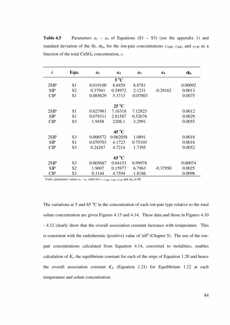
84
Table 4.5 Parameters a1 – a4 of Equations (S1 – S3) (see the appendix 1) and
standard deviation of the fit, σfit, for the ion-pair concentrations c2SIP, cSIP, and cCIP as a
function of the total CuSO4 concentration, c.
i Eqn. a1 a2 a3 a4 σσσσfit
5 oC
2SIP S1 0.019100 8.8459 8.8781 0.00092
SIP S2 0.37941 0.54972 2.1231 -0.29162 0.0013
CIP S1 0.085629 5.3713 -0.07803 0.0075
25 oC
2SIP S1 0.027981 7.16318 7.12925 0.0012
SIP S1 0.079311 2.81587 0.52676 0.0029
CIP S3 1.9458 2208.1 3.2991 0.0055
45 oC
2SIP S3 0.006572 0.062058 1.0891 0.0018
SIP S1 0.070703 4.1723 0.75103 0.0016
CIP S3 0.24267 4.7214 1.7395 0.0052
65 oC
2SIP S3 0.005687 0.04153 0.99978 0.00074
SIP S2 1.9697 0.15977 6.7963 -0.37950 0.0025
CIP S3 0.3144 4.7594 1.8186 0.0098
Units: parameter values a1 – a4 valid for c, c2SIP, cSIP, cCIP and σfit in M.
The variations at 5 and 65 oC in the concentration of each ion-pair type relative to the total
solute concentration are given Figures 4.13 and 4.14. These data and those in Figures 4.10
- 4.12 clearly show that the overall association constant increases with temperature. This
is consistent with the endothermic (positive) value of ∆Ho
(Chapter 5). The use of the ion-
pair concentrations calculated from Equation 4.14, converted to molalities, enables
calculation of Ki, the equilibrium constant for each of the steps of Equation 1.20 and hence
the overall association constant KA (Equation 1.21) for Equilibrium 1.22 at each
temperature and solute concentration.
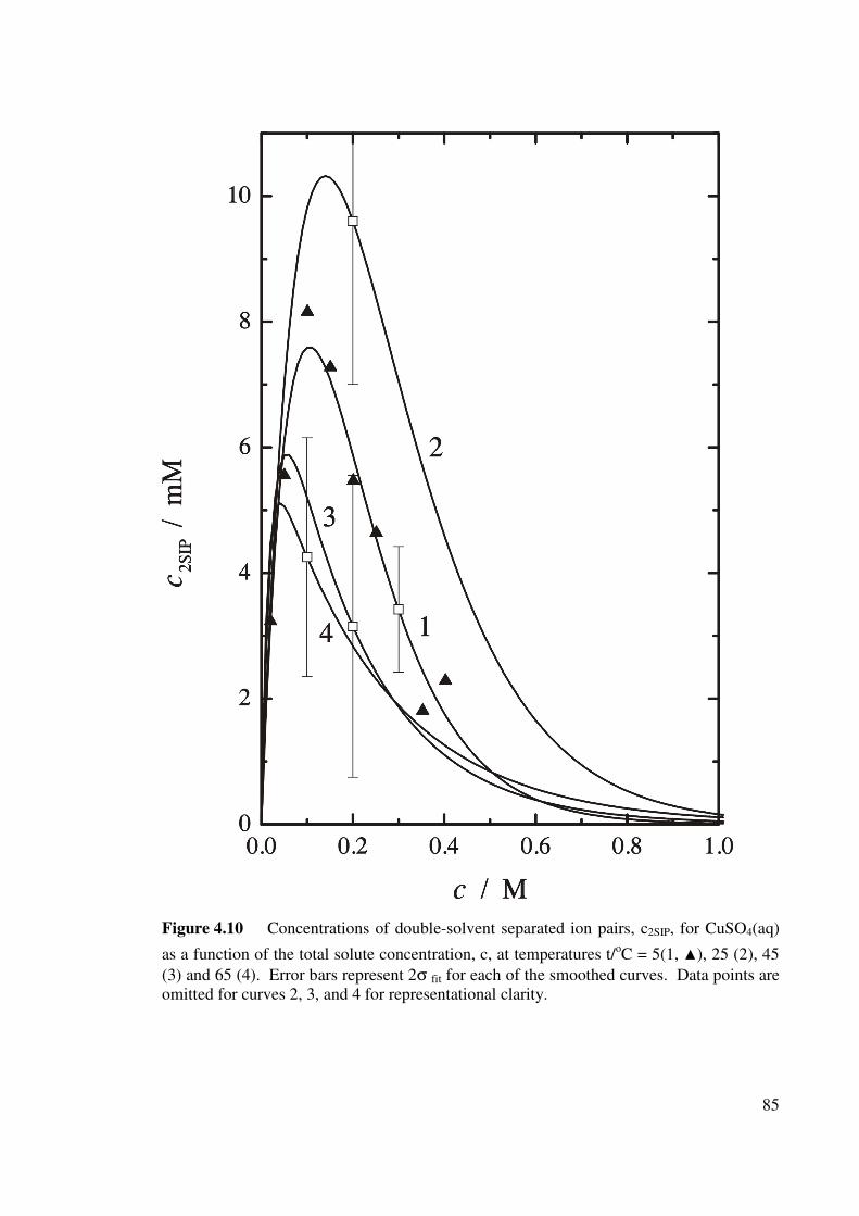
85
Figure 4.10 Concentrations of double-solvent separated ion pairs, c2SIP, for CuSO4(aq)
as a function of the total solute concentration, c, at temperatures t/oC = 5(1, ), 25 (2), 45
(3) and 65 (4). Error bars represent 2σ fit for each of the smoothed curves. Data points are
omitted for curves 2, 3, and 4 for representational clarity.
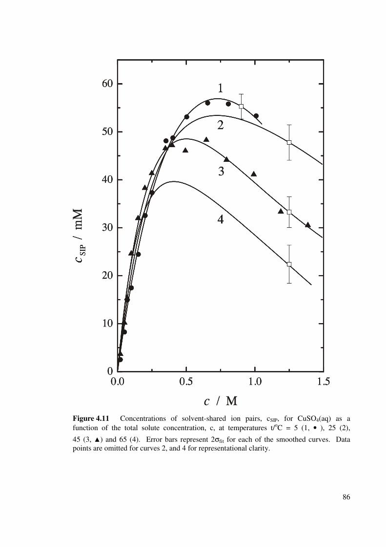
86
Figure 4.11 Concentrations of solvent-shared ion pairs, cSIP, for CuSO4(aq) as a
function of the total solute concentration, c, at temperatures t/oC = 5 (1, • ), 25 (2),
45 (3, ) and 65 (4). Error bars represent 2σfit for each of the smoothed curves. Data
points are omitted for curves 2, and 4 for representational clarity.
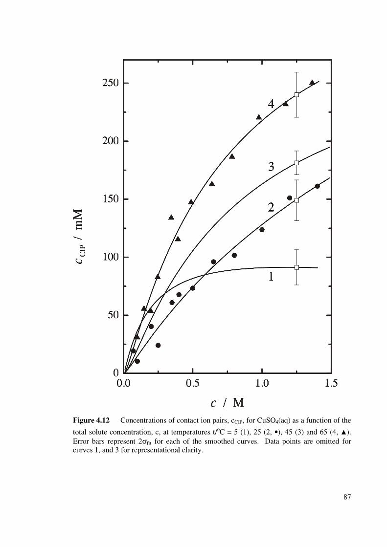
87
Figure 4.12 Concentrations of contact ion pairs, cCIP, for CuSO4(aq) as a function of the
total solute concentration, c, at temperatures t/oC = 5 (1), 25 (2, •), 45 (3) and 65 (4, ).
Error bars represent 2σfit for each of the smoothed curves. Data points are omitted for
curves 1, and 3 for representational clarity.
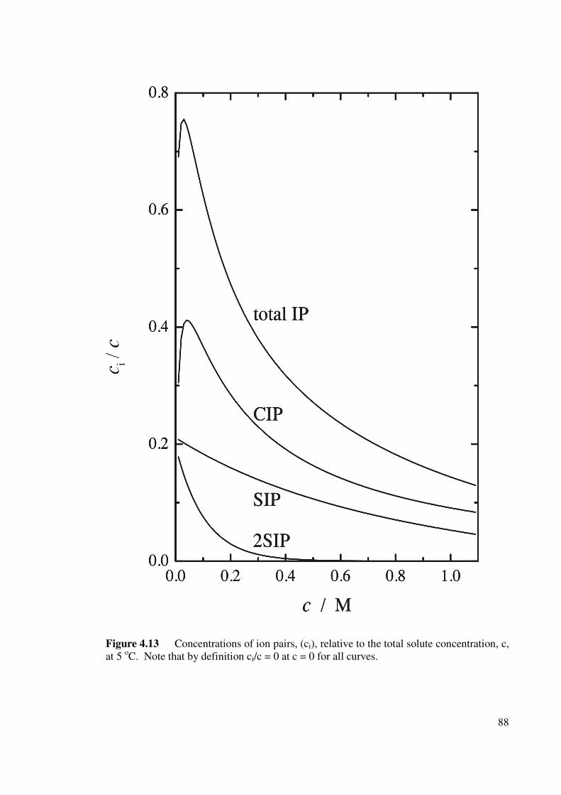
88
Figure 4.13 Concentrations of ion pairs, (ci), relative to the total solute concentration, c,
at 5 oC. Note that by definition ci/c = 0 at c = 0 for all curves.
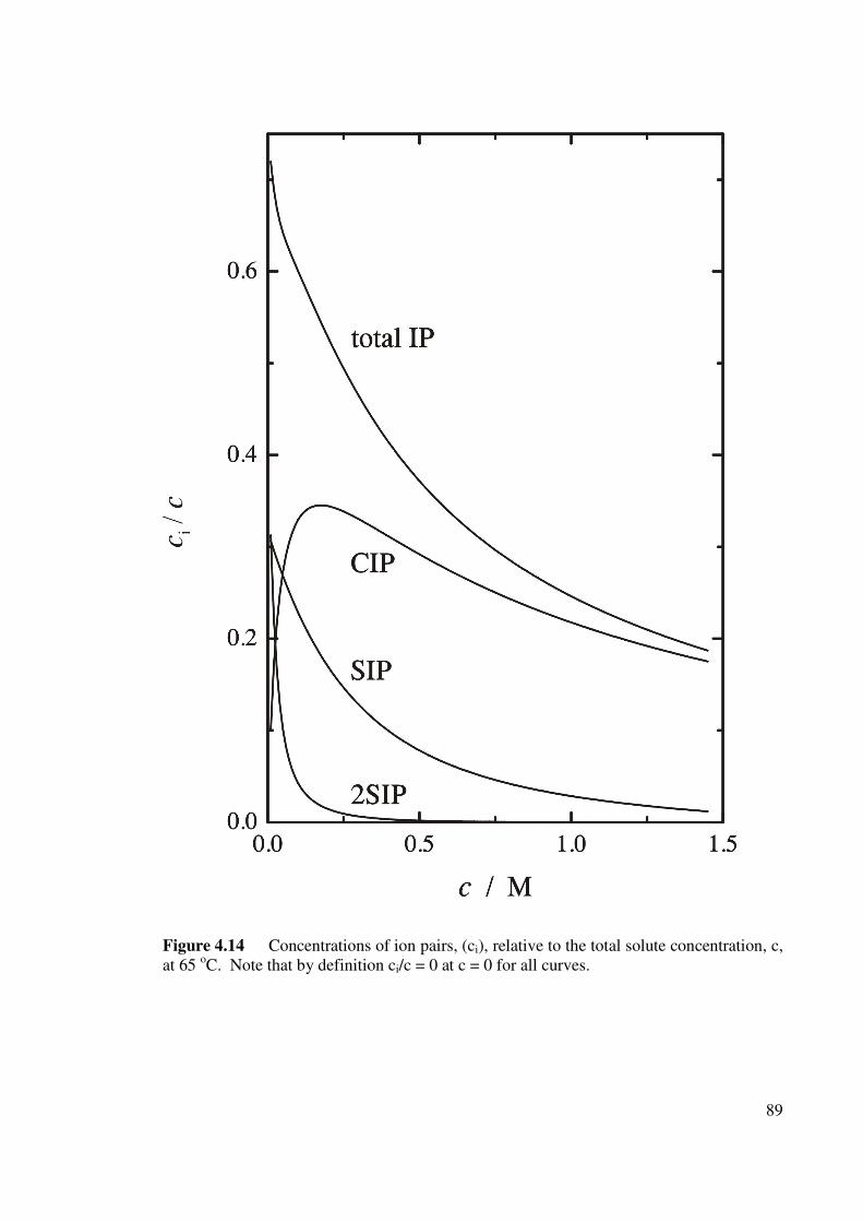
89
Figure 4.14 Concentrations of ion pairs, (ci), relative to the total solute concentration, c,
at 65 oC. Note that by definition ci/c = 0 at c = 0 for all curves.
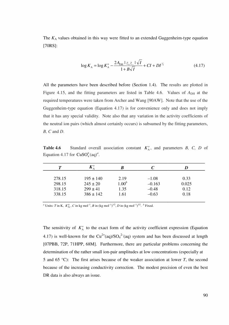
90
The KA values obtained in this way were fitted to an extended Guggenheim-type equation
[70RS]:
23
1
||2loglog DHo
AA DICIIB
IzzAKK ++
+−= −+ (4.17)
All the parameters have been described before (Section 1.4). The results are plotted in
Figure 4.15, and the fitting parameters are listed in Table 4.6. Values of ADH at the
required temperatures were taken from Archer and Wang [90AW]. Note that the use of the
Guggenheim-type equation (Equation 4.17) is for convenience only and does not imply
that it has any special validity. Note also that any variation in the activity coefficients of
the neutral ion pairs (which almost certainly occurs) is subsumed by the fitting parameters,
B, C and D.
Table 4.6 Standard overall association constant oKA , and parameters B, C, D of
Equation 4.17 for 0
4CuSO (aq)a.
T o
AK B C D
278.15 195 ± 140 2.19 –1.08 0.33
298.15 245 ± 20 1.00b –0.163 0.025
318.15 299 ± 41 1.35 –0.48 0.12
338.15 386 ± 142 1.61 –0.63 0.18
a Units: T in K, o
AK , C in kg mol–1, B in (kg mol–1)1/2, D in (kg mol–1)3/2. b Fixed.
The sensitivity of oKA to the exact form of the activity coefficient expression (Equation
4.17) is well-known for the Cu2+
(aq)/SO42–
(aq) system and has been discussed at length
[07PBB, 72P, 71HPP, 68M]. Furthermore, there are particular problems concerning the
determination of the rather small ion-pair amplitudes at low concentrations (especially at
5 and 65 °C): The first arises because of the weaker association at lower T, the second
because of the increasing conductivity correction. The modest precision of even the best
DR data is also always an issue.
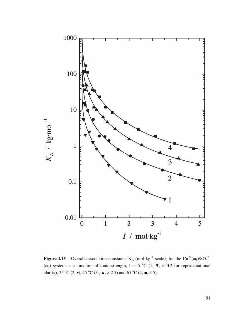
91
Figure 4.15 Overall association constants, KA (mol kg–1
scale), for the Cu2+
(aq)/SO42–
(aq) system as a function of ionic strength, I at 5 oC (1, , × 0.2 for representational
clarity), 25 oC (2, •), 45
oC (3 , , × 2.5) and 65
oC (4, , × 5).
92
Nevertheless, despite the uncertainty introduced by these factors the KA values obtained
are smooth and systematic functions of I at all temperatures (Figure 4.15).
As found for other systems [99BCH, 04BCH] the present values, valid for the ‘self-
medium’ of the pure electrolyte solutions, are lower at higher I than those measured in the
presence of a large excess of a supposedly indifferent electrolyte such as NaClO4 [07PBB].
This difference is usually attributed to activity coefficient effects [99BCH, 04BCH].
The values (on the mol kg–1
concentration scale) of the standard Gibbs energy, enthalpy,
entropy, and heat capacity changes for the overall association reaction (Equation 1.22)
were obtained from a conventional thermodynamic analysis of the )(o
A TK data based on
the equations
o
Aln KRTGo
−=∆ (4.18)
)]/ln([)()( o
p
o
298
o
p
o
298
o ∗∗∆+∆−−∆+∆=∆ TTCSTTTCHTG (4.19)
where T* = 298.15 K and o
pC∆ is assumed to be independent of temperature [07PBB].
The values derived in this way are presented in Table 4.7 along with the values obtained
from the most recent critical review [07PBB] and experimental investigation [05BBP].
Figure 4.16 shows that the values derived from the present study are in excellent
agreement with those recommended by IUPAC [07PBB] and with the most recent
experimental determination by Bešter-Rogač et al. [05BBP] (re-analyzed here in mol/kg
concentration units) employing high-precision conductivity measurements. Given the
large uncertainties in the DRS data, the agreement between the present and literature
values for the thermodynamic quantities, however gratifying, must be partly fortuitous.
This becomes apparent from a consideration of the stepwise equilibrium constants
(Equations 1.19(a-c)). Values of Ki were calculated from the smoothed species molalities
using the appropriate expressions (Equation 1.20).
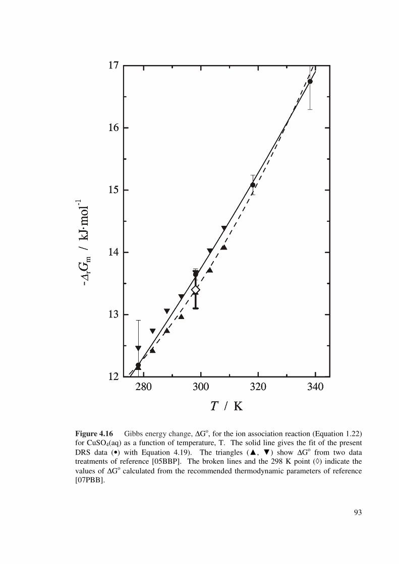
93
Figure 4.16 Gibbs energy change, ∆Go, for the ion association reaction (Equation 1.22)
for CuSO4(aq) as a function of temperature, T. The solid line gives the fit of the present
DRS data (•) with Equation 4.19). The triangles (, ) show ∆Go from two data
treatments of reference [05BBP]. The broken lines and the 298 K point (◊) indicate the
values of ∆Go calculated from the recommended thermodynamic parameters of reference
[07PBB].
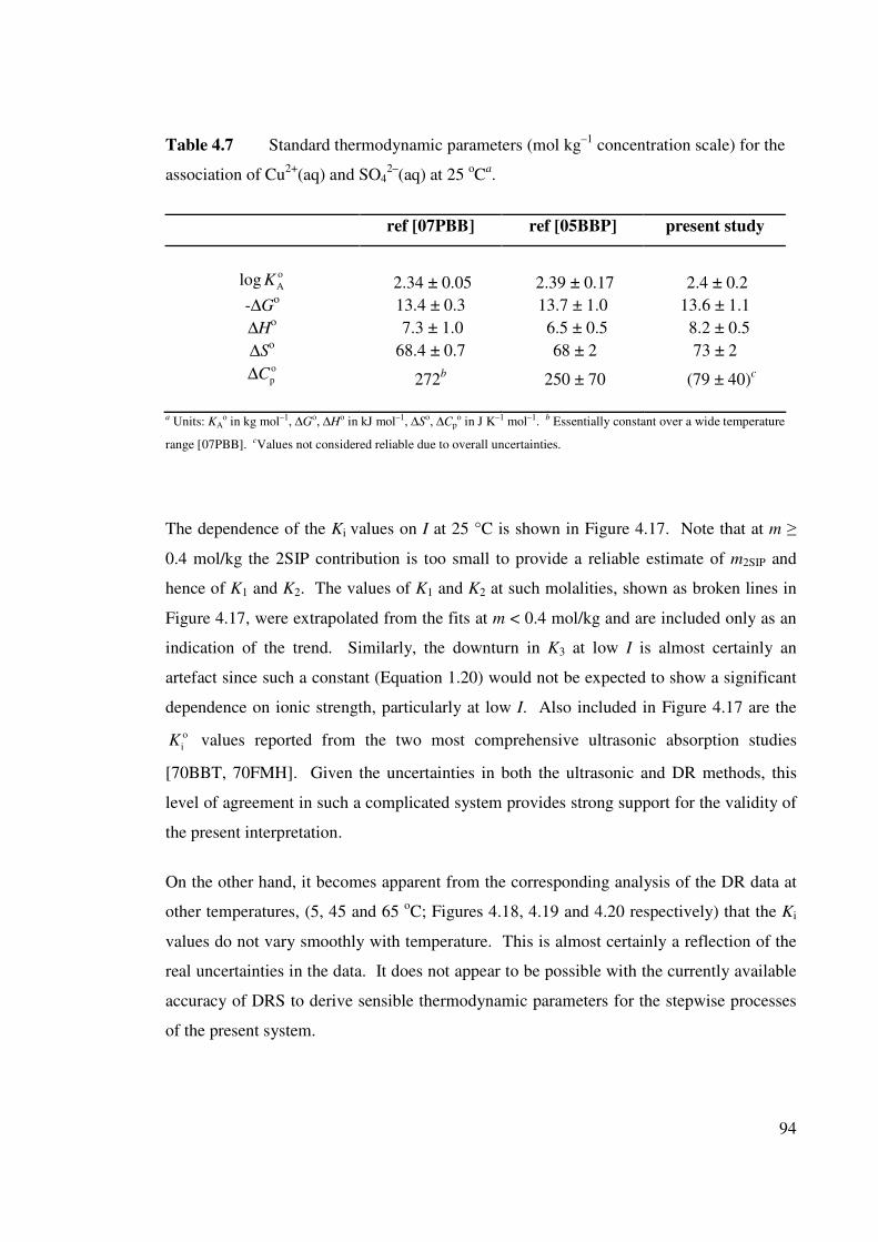
94
Table 4.7 Standard thermodynamic parameters (mol kg–1
concentration scale) for the
association of Cu2+
(aq) and SO42–
(aq) at 25 oC
a.
ref [07PBB] ref [05BBP] present study
o
Alog K 2.34 ± 0.05 2.39 ± 0.17 2.4 ± 0.2
-∆Go 13.4 ± 0.3 13.7 ± 1.0 13.6 ± 1.1
∆Ho 7.3 ± 1.0 6.5 ± 0.5 8.2 ± 0.5
∆So 68.4 ± 0.7 68 ± 2 73 ± 2
o
pC∆ 272b 250 ± 70 (79 ± 40)
c
a Units: KA
o in kg mol–1, ∆Go, ∆H
o in kJ mol–1, ∆So, ∆Cp
o in J K–1 mol–1. b Essentially constant over a wide temperature
range [07PBB]. cValues not considered reliable due to overall uncertainties.
The dependence of the Ki values on I at 25 °C is shown in Figure 4.17. Note that at m ≥
0.4 mol/kg the 2SIP contribution is too small to provide a reliable estimate of m2SIP and
hence of K1 and K2. The values of K1 and K2 at such molalities, shown as broken lines in
Figure 4.17, were extrapolated from the fits at m < 0.4 mol/kg and are included only as an
indication of the trend. Similarly, the downturn in K3 at low I is almost certainly an
artefact since such a constant (Equation 1.20) would not be expected to show a significant
dependence on ionic strength, particularly at low I. Also included in Figure 4.17 are the
o
iK values reported from the two most comprehensive ultrasonic absorption studies
[70BBT, 70FMH]. Given the uncertainties in both the ultrasonic and DR methods, this
level of agreement in such a complicated system provides strong support for the validity of
the present interpretation.
On the other hand, it becomes apparent from the corresponding analysis of the DR data at
other temperatures, (5, 45 and 65 oC; Figures 4.18, 4.19 and 4.20 respectively) that the Ki
values do not vary smoothly with temperature. This is almost certainly a reflection of the
real uncertainties in the data. It does not appear to be possible with the currently available
accuracy of DRS to derive sensible thermodynamic parameters for the stepwise processes
of the present system.
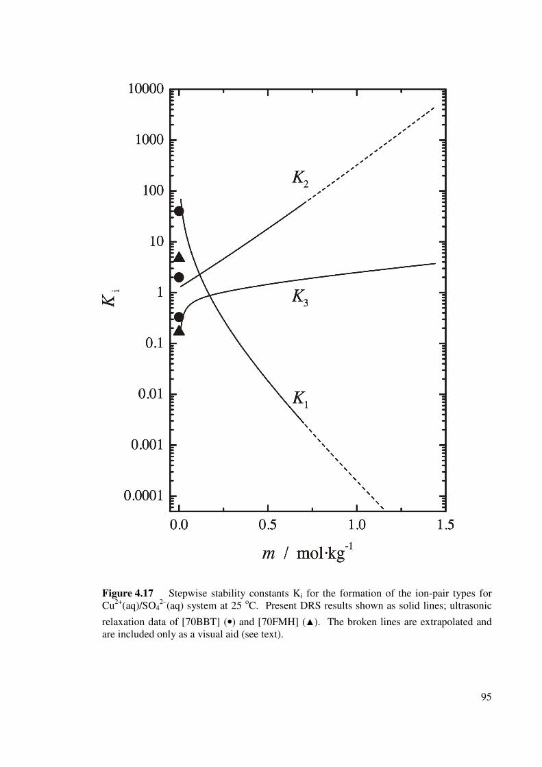
95
Figure 4.17 Stepwise stability constants Ki for the formation of the ion-pair types for
Cu2+
(aq)/SO42–
(aq) system at 25 oC. Present DRS results shown as solid lines; ultrasonic
relaxation data of [70BBT] (•) and [70FMH] (). The broken lines are extrapolated and
are included only as a visual aid (see text).
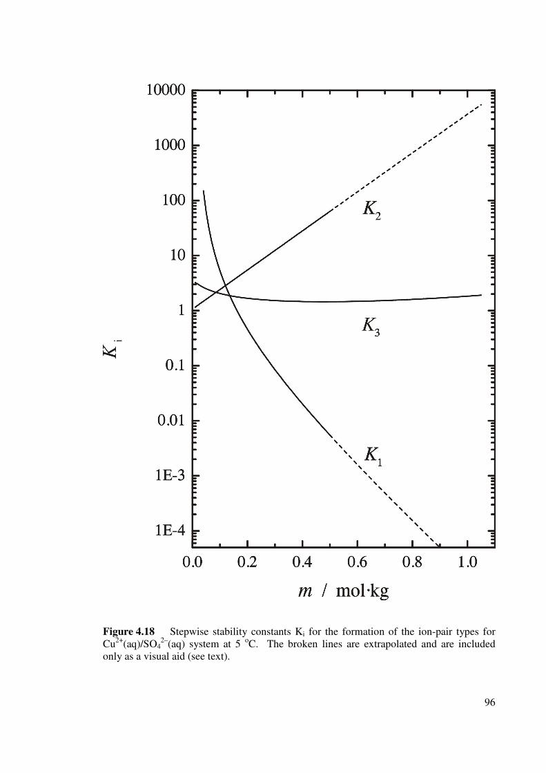
96
Figure 4.18 Stepwise stability constants Ki for the formation of the ion-pair types for
Cu2+
(aq)/SO42–
(aq) system at 5 oC. The broken lines are extrapolated and are included
only as a visual aid (see text).
97
Figure 4.19 Stepwise stability constants Ki for the formation of the ion-pair types for
Cu2+
(aq)/SO42–
(aq) system at 45 oC. The broken lines are extrapolated and are included
only as a visual aid (see text).
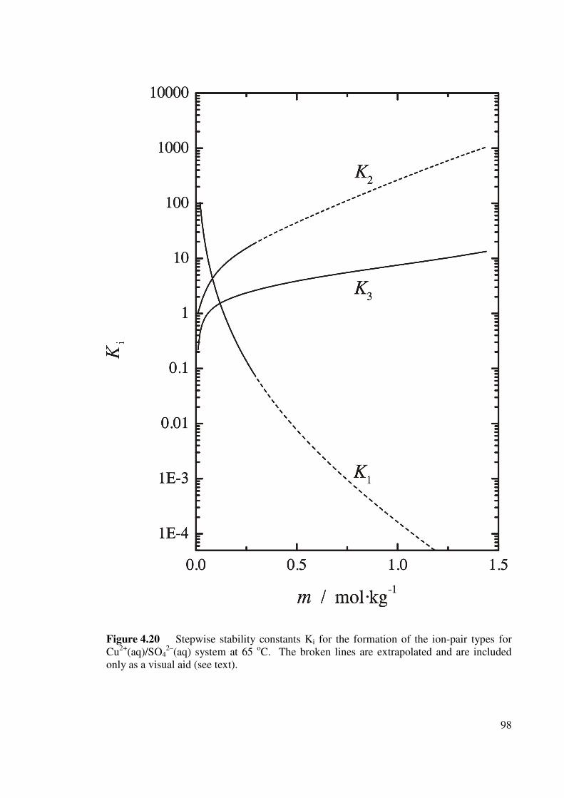
98
Figure 4.20 Stepwise stability constants Ki for the formation of the ion-pair types for
Cu2+
(aq)/SO42–
(aq) system at 65 oC. The broken lines are extrapolated and are included
only as a visual aid (see text).
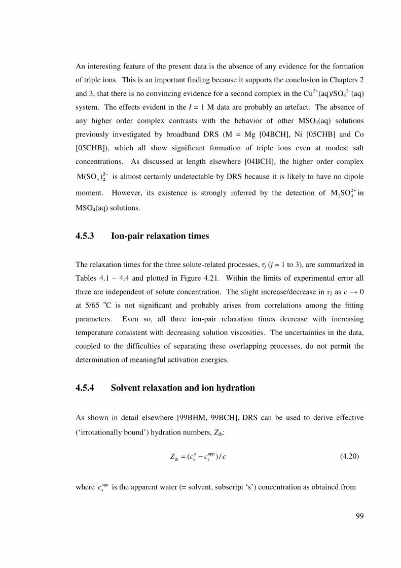
99
An interesting feature of the present data is the absence of any evidence for the formation
of triple ions. This is an important finding because it supports the conclusion in Chapters 2
and 3, that there is no convincing evidence for a second complex in the Cu2+
(aq)/SO42–
(aq)
system. The effects evident in the I = 1 M data are probably an artefact. The absence of
any higher order complex contrasts with the behavior of other MSO4(aq) solutions
previously investigated by broadband DRS (M = Mg [04BCH], Ni [05CHB] and Co
[05CHB]), which all show significant formation of triple ions even at modest salt
concentrations. As discussed at length elsewhere [04BCH], the higher order complex
−2
2)M(SO4 is almost certainly undetectable by DRS because it is likely to have no dipole
moment. However, its existence is strongly inferred by the detection of +2
42SOM in
MSO4(aq) solutions.
4.5.3 Ion-pair relaxation times
The relaxation times for the three solute-related processes, τj (j = 1 to 3), are summarized in
Tables 4.1 – 4.4 and plotted in Figure 4.21. Within the limits of experimental error all
three are independent of solute concentration. The slight increase/decrease in τ2 as c → 0
at 5/65 oC is not significant and probably arises from correlations among the fitting
parameters. Even so, all three ion-pair relaxation times decrease with increasing
temperature consistent with decreasing solution viscosities. The uncertainties in the data,
coupled to the difficulties of separating these overlapping processes, do not permit the
determination of meaningful activation energies.
4.5.4 Solvent relaxation and ion hydration
As shown in detail elsewhere [99BHM, 99BCH],
DRS can be used to derive effective
(‘irrotationally bound’) hydration numbers, Zib:
cccZ /)(app
s
o
sib −= (4.20)
where app
sc is the apparent water (= solvent, subscript ‘s’) concentration as obtained from
100
Figure 4.21 Solute relaxation times τ1, τ2 and τ3 for CuSO4(aq) at temperatures t/oC = 5
(,,), 25 (,,), (45 (,∆,), and 65(,,).
101
the DRS data and o
sc is the analytical (total) concentration of water in the solution. Values
of app
sc were calculated via the solvent-normalized Cavell equation
)()0(
)0(
))0(1(
))(1(
)(
)0(
1)0(2
1)(2s
s
o
s
2
ss
2
ssapp
s cSS
c
f
cf
c
cc ××
−
−××
+
+=
α
α
ε
ε
ε
ε (4.21)
as described in detail for MgSO4(aq) [04BCH], with correction for kinetic depolarization
of the ions assuming slip boundary conditions [99BHM, 99BCH]. As justified previously
[05CHB], the dispersion amplitude of unbound water in the CuSO4(aq) solutions:
∞−=+= εε454S )( SScS was derived by assuming )0(
∞∞= εε , the pure water value at the
appropriate temperature. The )0(∞
ε values were taken from Hölzl et al. [07HSB] and are
included in Tables 4.1 - 4.4 for convenience.
The values of Zib so obtained are plotted in Figure 4.22 and show that the total effective
solvation decreases smoothly with increasing concentration. The error bars correspond to
the standard deviation of the solvent amplitude obtained from fits of ∞
− εε 4 with
appropriate polynomials forced through the value for pure water, )0()0(∞
− εε . A striking
feature of the data in Figure 4.22 is the strong increase of the infinite dilution value, Zib(0),
with decreasing temperature. The trend from Zib(0) ≈ 41 at 5 °C to ≈ 29 at 25 °C, ≈ 22 at
45 °C, and ≈ 21 at 65 °C is consistent with the DRS solvation numbers reflecting a balance
between ion-solvent interactions and thermal motion.
The Zib(0) values substantially exceed the sum of the first-shell coordination numbers of
Cu2+
(CN+ ≈ 6 [93OR, 04RST]) and SO42–
(CN– ≈ 8 [93OR]) dictated by geometric
constraints. This indicates that water molecules beyond the first, and possibly even the
second, hydration shell of the ions are also restricted in their response to the imposed
electric field. At higher solute concentrations, Zib drops to values close to (5 and 25 °C) or
even below (45 and 65 °C) the sum of the first-shell coordination numbers (CN+ + CN–).
This is consistent with the breakdown of well-defined second hydration shells associated
with increased ion association and, in particular, with the increased formation of CIPs,
with rising temperature.
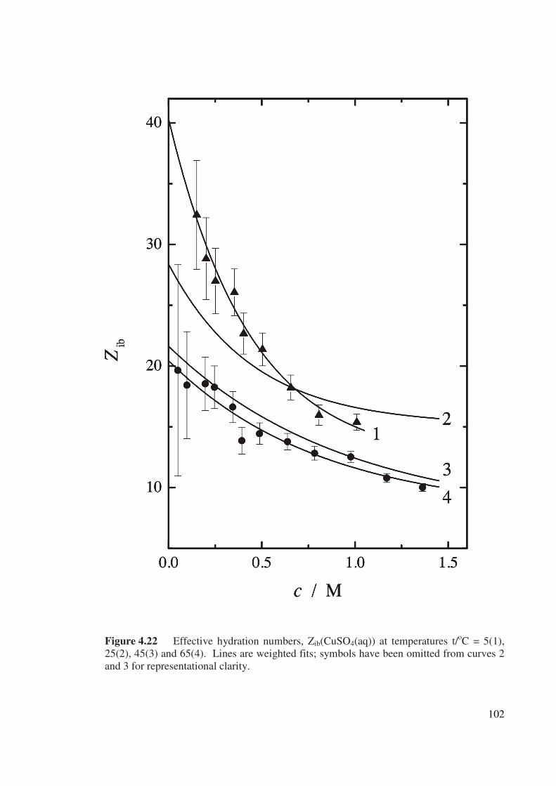
102
Figure 4.22 Effective hydration numbers, Zib(CuSO4(aq)) at temperatures t/oC = 5(1),
25(2), 45(3) and 65(4). Lines are weighted fits; symbols have been omitted from curves 2
and 3 for representational clarity.
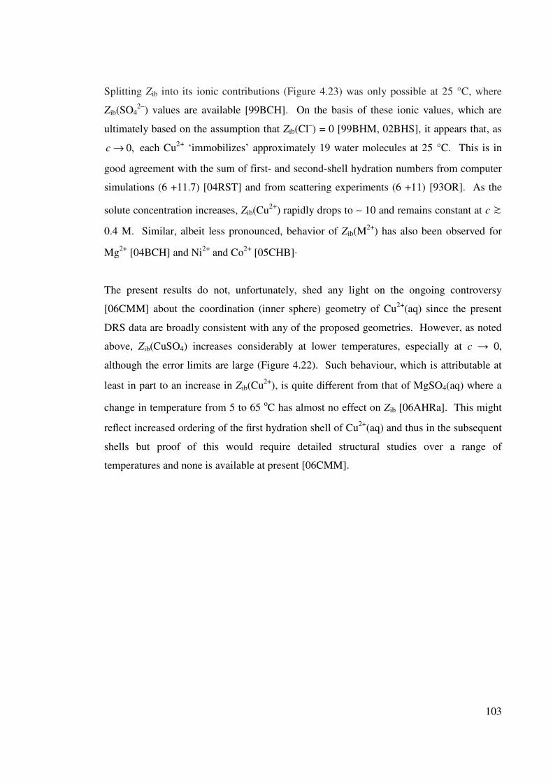
103
Splitting Zib into its ionic contributions (Figure 4.23) was only possible at 25 °C, where
Zib(SO42–
) values are available [99BCH]. On the basis of these ionic values, which are
ultimately based on the assumption that Zib(Cl–) = 0 [99BHM, 02BHS], it appears that, as
,0→c each Cu2+ ‘immobilizes’ approximately 19 water molecules at 25 °C. This is in
good agreement with the sum of first- and second-shell hydration numbers from computer
simulations (6 +11.7) [04RST] and from scattering experiments (6 +11) [93OR]. As the
solute concentration increases, Zib(Cu2+
) rapidly drops to ∼ 10 and remains constant at c
0.4 M. Similar, albeit less pronounced, behavior of Zib(M2+
) has also been observed for
Mg2+
[04BCH] and Ni2+
and Co2+
[05CHB].
The present results do not, unfortunately, shed any light on the ongoing controversy
[06CMM] about the coordination (inner sphere) geometry of Cu2+
(aq) since the present
DRS data are broadly consistent with any of the proposed geometries. However, as noted
above, Zib(CuSO4) increases considerably at lower temperatures, especially at c → 0,
although the error limits are large (Figure 4.22). Such behaviour, which is attributable at
least in part to an increase in Zib(Cu2+
), is quite different from that of MgSO4(aq) where a
change in temperature from 5 to 65 oC has almost no effect on Zib [06AHRa]. This might
reflect increased ordering of the first hydration shell of Cu2+
(aq) and thus in the subsequent
shells but proof of this would require detailed structural studies over a range of
temperatures and none is available at present [06CMM].
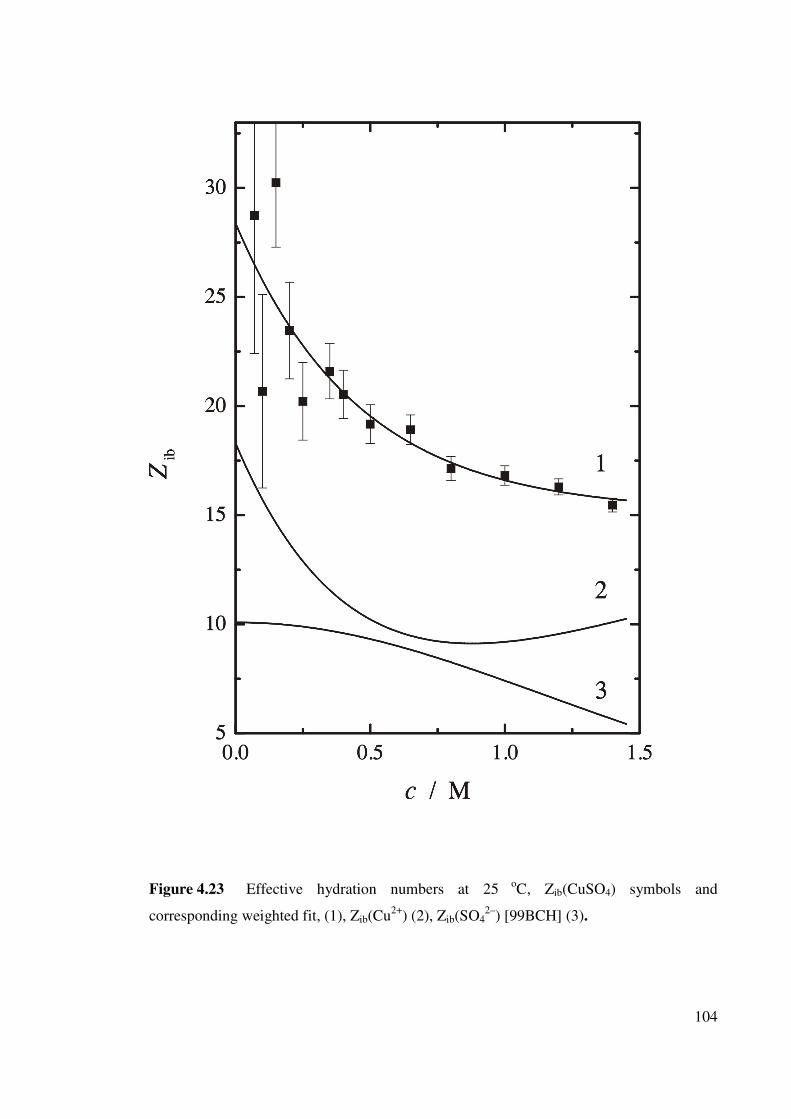
104
Figure 4.23 Effective hydration numbers at 25 o
C, Zib(CuSO4) symbols and
corresponding weighted fit, (1), Zib(Cu2+
) (2), Zib(SO42–
) [99BCH] (3).
105
4.6 IMPLICATIONS OF THE PRESENT WORK
The present DRS data clearly demonstrate that, as for MgSO4(aq) [04BCH], NiSO4(aq)
[05CHB], and CoSO4(aq) [05CHB], all three ion-pair types, 2SIPs, SIPs and CIPs, exist
simultaneously (in varying amounts) in aqueous solutions of copper(II) sulfate at all
practicable concentrations. The relative amounts of these species vary but all of them
persist over the temperature range studied (Figures 4.7 and 4.8). Where comparison is
possible, the present findings are quantitatively corroborated by earlier thermodynamic
(Figure 4.16) and ultrasonic absorption (Figure 4.17) studies.
The existence of such species explains many observations. For example, the failure of
early Raman spectroscopy studies [64HP] to detect ion association in CuSO4(aq) would
appear to be due not only to the relatively wide spectrometer slit-widths then available
(making observation of strongly overlapping peaks difficult) but also because the species
formed were mostly solvent-separated ion pairs (2SIPs and SIPs) that are not usually
detected by Raman measurements of the strong ν1(a1) mode of the SO42–
ion [03RIH].
Modern high-quality Raman spectra [06He, 08RIH] detect CIP concentrations that are in
broad agreement with the present DRS results.
The difficulties experienced in obtaining a unique theoretical description of even the most
high quality conductivity data [71HPP, 05BBP] are also closely related to the presence of
solvent-separated ion pairs. This is because such species make difficult the meaningful
definition of the integration limits (distance parameters) that are required by the theoretical
fitting equations [83J]. Similar considerations apply to the estimation of activity
coefficients, a problem that has been recognized for at least 50 years and which has led at
least one authoritative investigator to suggest that “it may become desirable to adopt
reasonable but arbitrary conventions which would make K values unambiguous [72P].” As
noted previously [04BCH], activity coefficient equations that take no account of the actual
species present cannot be much more than exercises in numerology, with little physical
significance.
The existence of solvent-separated ion pairs also explains why the KA and o
AK values that
106
have been obtained from extensive high quality measurements of the Cu2+
(aq)/SO42–
(aq)
system by UV-Visible spectrophotometry are lower than those obtained from reliable
conductivity and thermodynamic data (Chapters 2 and 3) [07PBB, 06He].
Finally, although not the focus of the present study, the presence of the various ion-pair
types is of considerable significance in kinetic studies. Not only would such species be
expected to affect homogeneous reaction kinetics involving CuSO4(aq) but, potentially
much more importantly, the heterogeneous kinetics involved for example in the
electrodissolution and electrodeposition steps of the copper refining process.
107
Chapter Five
Calorimetry of the Cu2+
/SO42–
interaction
Studies of metal/ligand interactions such as that between Cu2+
(aq) and SO42–
(aq) have
mostly involved only measurements of the association constants or Gibbs energy change
(Chapters 2 and 3). However, greater insights into the interactions taking place can be
obtained by dividing ∆Go into its component enthalpy and entropy changes, ∆H
o and ∆S
o,
since
∆Go = –RT lnK
o = ∆H
o – T∆S
o (5.1)
The enthalpy change associated with complex formation in the Cu2+
(aq)/SO42–
(aq) system
has been studied by many authors using various techniques. These data have been
presented in Table 1.2 but for convenience they are repeated here as Table 5.1. This table
shows that ∆Ho has been moderately well characterized at infinite dilution by calorimetry,
and by the variation of the overall association constant with temperature (the ‘K(T)’ or
van’t Hoff method). The calorimetric studies [69BG, 69IEC, 69IECa, 70L, 73HP, 73P]
used three similar but different methods. These are: (a) the simultaneous determination of
KA and ∆H by titration calorimetry (the so-called entropy titration technique) [69BG,
69IEC, 73P], (b) ∆H calculated from calorimetric titration data using an independently
determined KA value, [73HP, 73P] and (c) heat of dilution measurements [70L, 72P].
In the entropy titration method, the heat of complexation, Qc is measured as a function of
[Cu2+
] and [SO42–
] and standard computational techniques are then used to calculate
(optimize) KA and ∆H simultaneously [63LZ, 66CIH, 67AP, 72ECI, 89ACM]. Although
it is in principle possible to determine both KA and ∆H of a reaction in solution in this way
[66CIH, 68IES], there are certain disadvantages and limitations to this method.
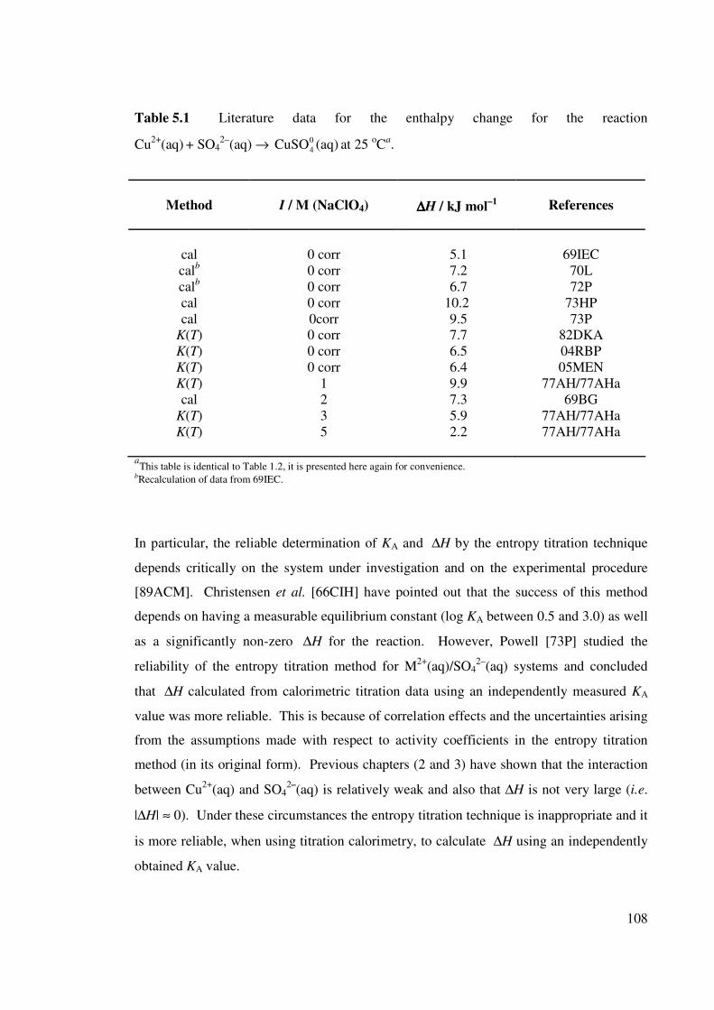
108
Table 5.1 Literature data for the enthalpy change for the reaction
Cu2+
(aq) + SO42–
(aq) → 0
4CuSO (aq) at 25 oC
a.
Method
I / M (NaClO4)
∆∆∆∆H / kJ mol–1
References
cal
calb
calb
cal
cal
K(T)
K(T)
K(T)
K(T)
cal
K(T)
K(T)
0 corr
0 corr
0 corr
0 corr
0corr
0 corr
0 corr
0 corr
1
2
3
5
5.1
7.2
6.7
10.2
9.5
7.7
6.5
6.4
9.9
7.3
5.9
2.2
69IEC
70L
72P
73HP
73P
82DKA
04RBP
05MEN
77AH/77AHa
69BG
77AH/77AHa
77AH/77AHa
aThis table is identical to Table 1.2, it is presented here again for convenience.
bRecalculation of data from 69IEC.
In particular, the reliable determination of KA and ∆H by the entropy titration technique
depends critically on the system under investigation and on the experimental procedure
[89ACM]. Christensen et al. [66CIH] have pointed out that the success of this method
depends on having a measurable equilibrium constant (log KA between 0.5 and 3.0) as well
as a significantly non-zero ∆H for the reaction. However, Powell [73P] studied the
reliability of the entropy titration method for M2+
(aq)/SO42–
(aq) systems and concluded
that ∆H calculated from calorimetric titration data using an independently measured KA
value was more reliable. This is because of correlation effects and the uncertainties arising
from the assumptions made with respect to activity coefficients in the entropy titration
method (in its original form). Previous chapters (2 and 3) have shown that the interaction
between Cu2+
(aq) and SO42–
(aq) is relatively weak and also that ∆H is not very large (i.e.
|∆H| ≈ 0). Under these circumstances the entropy titration technique is inappropriate and it
is more reliable, when using titration calorimetry, to calculate ∆H using an independently
obtained KA value.
109
In the heat of dilution method, the variation of ∆dilH of an electrolyte with concentration is
fitted with an appropriate activity coefficient model, typically an extended Debye-Hückel
equation, plus an ion association term to obtain the ∆Ho value. Since accurate heat of
dilution data can in principle be measured down to very low concentrations, this method is
able to produce reliable estimates of ∆Ho. In principle, heat of dilution data could also be
used to calculate o
AK and ∆Ho by an appropriate optimization procedure. However,
Larson (70L) noted that the KA values determined in this way were less accurate than those
obtained by any of the common methods. The value of ∆Ho obtained is again critically
dependent on the exact form of the activity coefficient equation adopted. Another
disadvantage of ∆dilH measurements is that they are restricted to a single ratio of the
interacting ions since it is the salt solution, in this case CuSO4(aq), which is being diluted.
Such measurements are therefore unsuited for determining ∆H at finite ionic strengths or if
higher order complexes are present.
As already noted, the standard ∆Ho for the association of Cu
2+(aq) with SO4
2–(aq) is,
moderately well characterized (Table 5.1). Nevertheless, given the apparent simplicity of
the reaction, the ∆Ho values show an unsatisfactory spread. The reasons for this spread are
not clear. As noted by Powell et al. [07PBB] there are a number of possible factors
including variation in the KA value adopted by different authors.
In contrast to the plethora of ∆Ho values obtained from measurements in dilute solutions,
there is only one study of ∆H as function of I. Unfortunately, this study employed the K(T)
method, which is generally considered to be less reliable than direct calorimetric
measurements due to the errors involved in taking the derivative of the log KA against 1/T
plot [57N] and the presence of unsuspected temperature dependent errors in K(T). In other
words there is virtually no reliable information on the ionic strength dependence of ∆H and
∆S for the Cu2+
(aq)/SO42–
(aq) system. Thus, a thorough investigation of the effects of
ionic strength dependence of ∆H was undertaken as part of the present work.
110
5.1 APPLICATION OF TITRATION CALORIMETRY TO
M2+
/SO42–
ASSOCIATION
There is a wide range of calorimeter types [78FC, 79KF] and methods available for
measuring the enthalpy changes accompanying complex formation. The particular
calorimeter and the method chosen depend on the system being investigated. Titration
calorimetry employing isothermal calorimeters is a powerful and versatile technique that
can provide reliable thermodynamic information on reactions in solutions [83Wa, 84N,
99V, 03C]. The advantages of this technique over the more common isoperibol
calorimeters are that large amounts of information can be obtained in a single experimental
run, no heat capacity measurements (or corrections) are required and also no corrections
are necessary for the heat exchange between reaction vessel and its environment [73CHE].
In titration calorimetry, the heat generated or absorbed by a chemically reacting system is
recorded as a function of the amount of added reactant. Thus, the amount of heat is
characterized by a direct proportionality between energy evolved or absorbed and the
amount of product formed [94MO]. Consider the formation of the complex 0
4MSO (aq)
from M2+
(aq) and SO42–
(aq). The reaction under consideration can be written as,
M2+
(aq) + SO42–
(aq) 0
4MSO (aq) (5.2)
and the overall formation constant KA in terms of concentration (molarity or molality) can
be deduced as in Chapters 2 and 3 using the same the assumption.
KA =]SO][M[
][MSO2
4
2
0
4
−+ (5.3)
Assuming Equilibrium 5.2 is the only significant process occurring, i.e., that there is no
formation of higher associates such as −2
24 )M(SO or any other species, the heat of
complexation, Qc, can be given [68CG] as
111
∑−= HVQ ∆]MSO[0
4c (5.4)
where V is the total volume of the solution, [ 0
4MSO ] is the concentration of the complex
formed and ∆H is the accompanying enthalpy change [66PVA].
The heat of complexation is obtained by subtracting from the overall heat effect, Qobs,
those heat effects, ∑ exQ , that are extraneous to the reaction. Such effects include heats of
dilution, Qd, the heat of stirring, etc. [68CG].
∑−= exobsc QQQ (5.5)
In the present context, all species are present in homogeneous solution and the stirring rate
is constant throughout and thus dex QQ ≈∑ . Therefore Equation 5.5 can be written as
dobsc QQQ −≈ (5.6)
The number of moles of the complex formed can be obtained from the initial
concentrations, volumes of the reagents and the equilibrium constant for the complexation
reaction. For the formation of 0
4CuSO using appropriate mass balance equations, Equation
5.4 can be written with known parameters to calculate the ∆H [66CIH, 66PVA]:
1/22
4
222
4
22
4
2
c
]][SOCu[4)/1][SO]Cu([)/1]][SOCu([
/2∆
−+−+−+−++−+
−=
KK
VQH (5.7)
Values of the entropy change, ∆S of the reaction can be calculated from the relationship
between the Gibbs energy change and the enthalpy change (Equation 5.1).
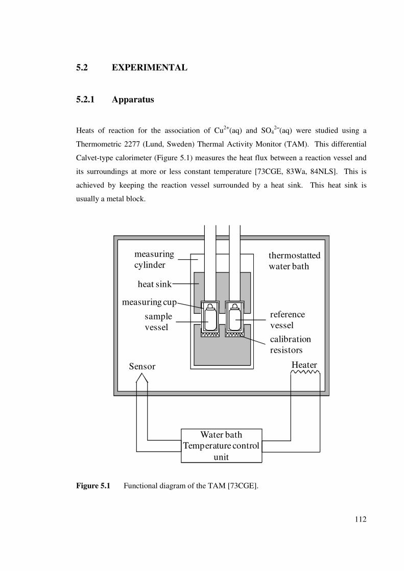
112
5.2 EXPERIMENTAL
5.2.1 Apparatus
Heats of reaction for the association of Cu2+
(aq) and SO42–
(aq) were studied using a
Thermometric 2277 (Lund, Sweden) Thermal Activity Monitor (TAM). This differential
Calvet-type calorimeter (Figure 5.1) measures the heat flux between a reaction vessel and
its surroundings at more or less constant temperature [73CGE, 83Wa, 84NLS]. This is
achieved by keeping the reaction vessel surrounded by a heat sink. This heat sink is
usually a metal block.
Water bath
Temperature control
unit
HeaterSensor
thermostatted
water bath
reference
vessel
calibration
resistors
sample
vessel
measuring cup
heat sink
measuring
cylinder
Figure 5.1 Functional diagram of the TAM [73CGE].
113
The calorimeter sensor, consisting of a multijunction thermopile made with semi-
conducting Peltier-effect plates [91BW], is placed between the reaction vessel and the heat
sink (Figure 5.2). The heat produced or absorbed during a reaction is transferred from or
to the reaction vessel through the thermopile to the heat sink/source system so as to re-
establish thermal equilibrium [03C]. Ideally, all heat exchange occurs between the
reaction vessel and the heat sink through the thermopile [91BW]. When a reaction occurs,
the temperature gradient between the reaction vessel and the sink/source is proportional to
the voltage signal of the thermopiles. This voltage signal is amplified and recorded [03C].
A precisely thermostatted calorimeter vessel and heat sink enable heat changes of less than
one microwatt to be detected. This exceptional thermal stability is achieved by utilizing a
water bath surrounding the measuring vessels (Figure 5.1) and acting as an infinite heat
sink [91BW]. As a result, the TAM can provide very sensitive measurements of heats of
reaction. The Digitam 4.1 software package provides interactive control of the TAM,
injection volumes, etc., as well as the calculation of heat loss or gain during the experiment
[03C]. To achieve accuracy in the corrected heat change, the titration calorimeter must be
calibrated and tested immediately before initiating an experiment.
5.2.2 Electrical calibration
Electrical calibration is performed by adding an accurately-known amount of energy to the
calorimeter via a resistance heater. The current through the heater is determined by
measuring the potential difference across a standard resistor held at constant temperature,
which is in series with the calibration heater. This allows calculation of the amount of
energy supplied by the calibration heater. The precision of the instrument can be obtained
by repeat calibration runs [94MO].
Electrical calibration is a convenient, precise method to determine the heat equivalent of a
calorimeter [01WG]. However, a calibration heater may produce a different heat flow
pattern than that caused by a chemical reaction, which may give rise to a significantly
different temperature distribution in the reaction vessel. In practical measurements, this
may produce in turn a different response in the thermopile (for the same quantity of heat),
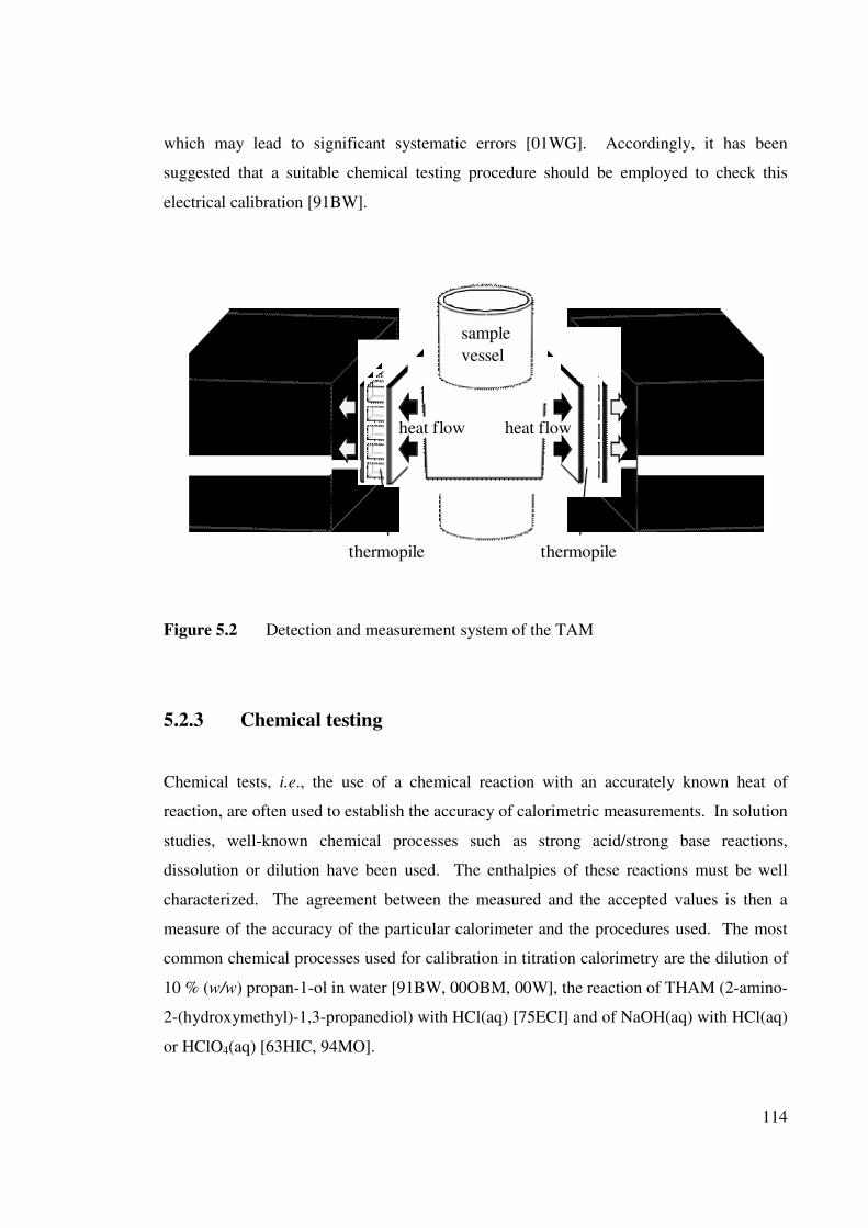
114
which may lead to significant systematic errors [01WG]. Accordingly, it has been
suggested that a suitable chemical testing procedure should be employed to check this
electrical calibration [91BW].
Heat sinkHeat sink
thermopile thermopile
heat flow heat flow
sample
vessel
Figure 5.2 Detection and measurement system of the TAM
5.2.3 Chemical testing
Chemical tests, i.e., the use of a chemical reaction with an accurately known heat of
reaction, are often used to establish the accuracy of calorimetric measurements. In solution
studies, well-known chemical processes such as strong acid/strong base reactions,
dissolution or dilution have been used. The enthalpies of these reactions must be well
characterized. The agreement between the measured and the accepted values is then a
measure of the accuracy of the particular calorimeter and the procedures used. The most
common chemical processes used for calibration in titration calorimetry are the dilution of
10 % (w/w) propan-1-ol in water [91BW, 00OBM, 00W], the reaction of THAM (2-amino-
2-(hydroxymethyl)-1,3-propanediol) with HCl(aq) [75ECI] and of NaOH(aq) with HCl(aq)
or HClO4(aq) [63HIC, 94MO].
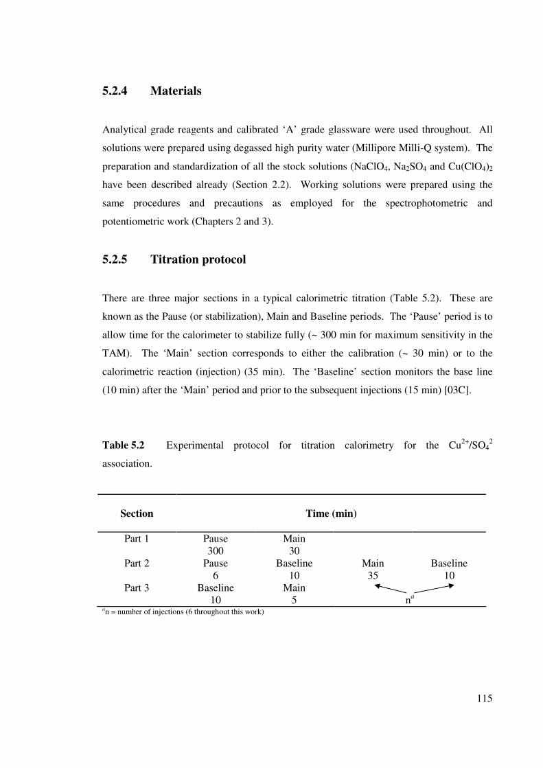
115
5.2.4 Materials
Analytical grade reagents and calibrated ‘A’ grade glassware were used throughout. All
solutions were prepared using degassed high purity water (Millipore Milli-Q system). The
preparation and standardization of all the stock solutions (NaClO4, Na2SO4 and Cu(ClO4)2
have been described already (Section 2.2). Working solutions were prepared using the
same procedures and precautions as employed for the spectrophotometric and
potentiometric work (Chapters 2 and 3).
5.2.5 Titration protocol
There are three major sections in a typical calorimetric titration (Table 5.2). These are
known as the Pause (or stabilization), Main and Baseline periods. The ‘Pause’ period is to
allow time for the calorimeter to stabilize fully (~ 300 min for maximum sensitivity in the
TAM). The ‘Main’ section corresponds to either the calibration (~ 30 min) or to the
calorimetric reaction (injection) (35 min). The ‘Baseline’ section monitors the base line
(10 min) after the ‘Main’ period and prior to the subsequent injections (15 min) [03C].
Table 5.2 Experimental protocol for titration calorimetry for the Cu2+
/SO42
association.
Section
Time (min)
Part 1 Pause
300
Main
30
Part 2 Pause
6
Baseline
10
Main
35
Baseline
10
Part 3 Baseline
10
Main
5
na
an = number of injections (6 throughout this work)
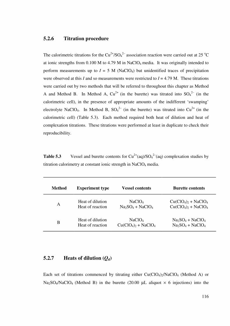
116
5.2.6 Titration procedure
The calorimetric titrations for the Cu2+
/SO42–
association reaction were carried out at 25 oC
at ionic strengths from 0.100 M to 4.79 M in NaClO4 media. It was originally intended to
perform measurements up to I = 5 M (NaClO4) but unidentified traces of precipitation
were observed at this I and so measurements were restricted to I = 4.79 M. These titrations
were carried out by two methods that will be referred to throughout this chapter as Method
A and Method B. In Method A, Cu2+
(in the burette) was titrated into SO42–
(in the
calorimetric cell), in the presence of appropriate amounts of the indifferent ‘swamping’
electrolyte NaClO4. In Method B, SO42–
(in the burette) was titrated into Cu2+
(in the
calorimetric cell) (Table 5.3). Each method required both heat of dilution and heat of
complexation titrations. These titrations were performed at least in duplicate to check their
reproducibility.
Table 5.3 Vessel and burette contents for Cu2+
(aq)/SO42–
(aq) complexation studies by
titration calorimetry at constant ionic strength in NaClO4 media.
Method Experiment type
Vessel contents
Burette contents
A Heat of dilution
Heat of reaction
NaClO4
Na2SO4 + NaClO4
Cu(ClO4)2 + NaClO4
Cu(ClO4)2 + NaClO4
B Heat of dilution
Heat of reaction
NaClO4
Cu(ClO4)2 + NaClO4
Na2SO4 + NaClO4
Na2SO4 + NaClO4
5.2.7 Heats of dilution (Qd)
Each set of titrations commenced by titrating either Cu(ClO4)2/NaClO4 (Method A) or
Na2SO4/NaClO4 (Method B) in the burette (20.00 µL aliquot × 6 injections) into the
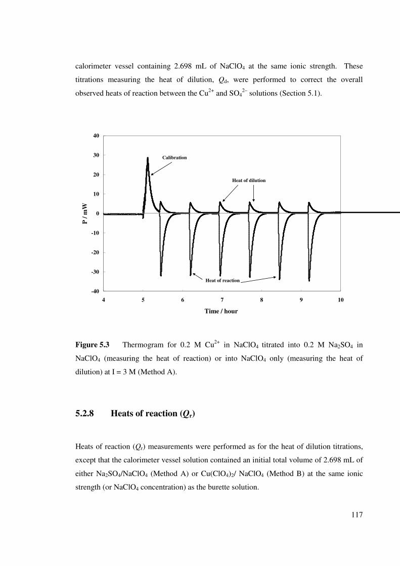
117
calorimeter vessel containing 2.698 mL of NaClO4 at the same ionic strength. These
titrations measuring the heat of dilution, Qd, were performed to correct the overall
observed heats of reaction between the Cu2+
and SO42–
solutions (Section 5.1).
-40
-30
-20
-10
0
10
20
30
40
4 5 6 7 8 9 10
Time / hour
P /
mW
Heat of dilution
Calibration
Heat of reaction
Figure 5.3 Thermogram for 0.2 M Cu2+
in NaClO4 titrated into 0.2 M Na2SO4 in
NaClO4 (measuring the heat of reaction) or into NaClO4 only (measuring the heat of
dilution) at I = 3 M (Method A).
5.2.8 Heats of reaction (Qr)
Heats of reaction (Qr) measurements were performed as for the heat of dilution titrations,
except that the calorimeter vessel solution contained an initial total volume of 2.698 mL of
either Na2SO4/NaClO4 (Method A) or Cu(ClO4)2/ NaClO4 (Method B) at the same ionic
strength (or NaClO4 concentration) as the burette solution.
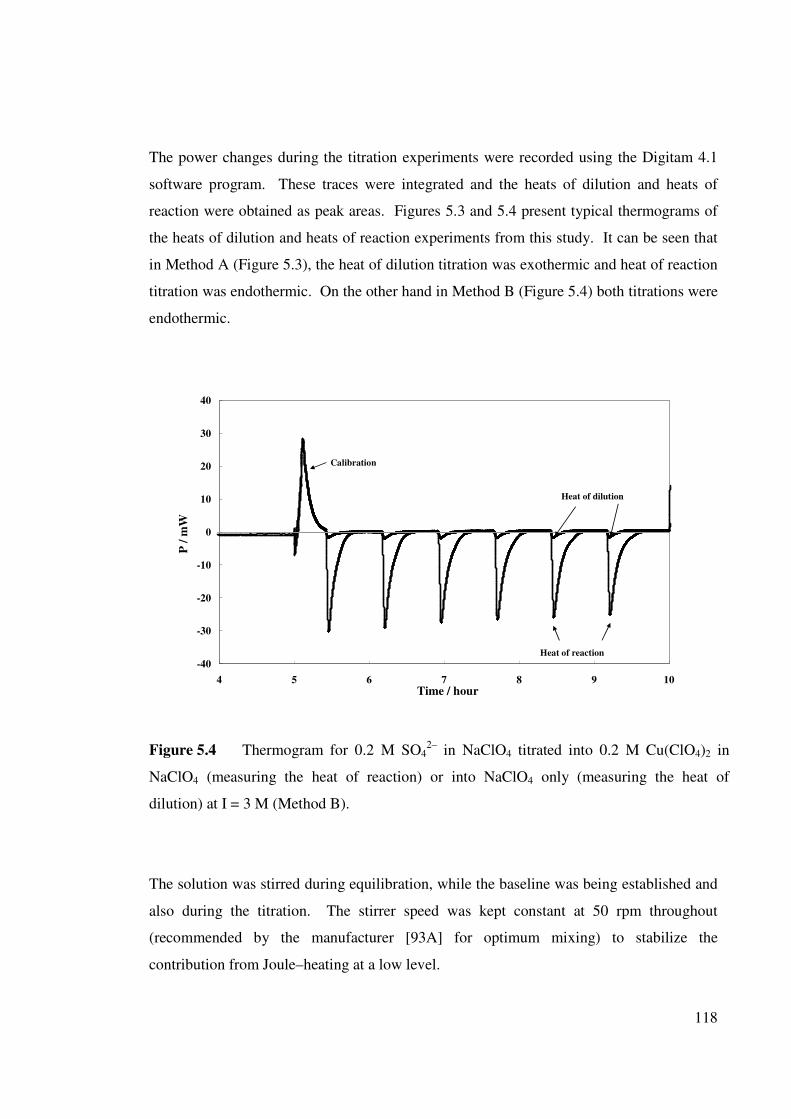
118
The power changes during the titration experiments were recorded using the Digitam 4.1
software program. These traces were integrated and the heats of dilution and heats of
reaction were obtained as peak areas. Figures 5.3 and 5.4 present typical thermograms of
the heats of dilution and heats of reaction experiments from this study. It can be seen that
in Method A (Figure 5.3), the heat of dilution titration was exothermic and heat of reaction
titration was endothermic. On the other hand in Method B (Figure 5.4) both titrations were
endothermic.
-40
-30
-20
-10
0
10
20
30
40
4 5 6 7 8 9 10Time / hour
P /
mW
Heat of dilution
Calibration
Heat of reaction
Figure 5.4 Thermogram for 0.2 M SO42–
in NaClO4 titrated into 0.2 M Cu(ClO4)2 in
NaClO4 (measuring the heat of reaction) or into NaClO4 only (measuring the heat of
dilution) at I = 3 M (Method B).
The solution was stirred during equilibration, while the baseline was being established and
also during the titration. The stirrer speed was kept constant at 50 rpm throughout
(recommended by the manufacturer [93A] for optimum mixing) to stabilize the
contribution from Joule–heating at a low level.
119
When the solution and the calorimeter vessel were in thermal equilibrium, a ‘dynamic’
calibration (of the resistors) was performed before initiating the titration. An injection
speed of 0.1 µL s–1
was selected to achieve the best reproducibility [03C]. The injection
volume was calibrated at each ionic strength before commencing the titrations by weighing
repeat injection volumes into a capped vial and calculating the exact volume using the
known densities of the solutions. Six successive aliquots of 20 µL were injected into the
vessel in each run. Each injection was kept 10 min apart to enable the instrument to reach
pseudo-equilibrium prior to the next injection. To avoid the heat changes due to the
interaction with species such as HSO4–, the pH of titrant and titrand were measured and if
necessary adjusted to 4.50 ± 0.03 by adding appropriate (minute) amounts of either
concentrated HClO4 or NaOH.
Ideally, in calorimetric titrations performed in a constant ionic medium, the interacting
species will be at far lower concentrations than the ‘swamping electrolyte’ (in this case
NaClO4). In this way the activity coefficients of the interacting species will be held
constant. However, this cannot be achieved in practice for the Cu2+
/SO42–
system because
both ∆H (Table 5.1) and KA (Table 1.1) are fairly small. Thus, to achieve measurable heat
effects, it is necessary to use relatively high concentrations of either or both Cu2+
or SO42–
.
It is therefore necessary, in both Method A and Method B titrations, to replace a relatively
large fraction of the swamping electrolyte by the interacting species. This less-than-
optimal, but inescapable, situation inevitably creates a number of problems which are
discussed further below. Table 5.4 summarizes the approximate concentrations of
Cu(ClO4)2, Na2SO4 and NaClO4 used in this study.
5.3 RESULTS AND DISCUSSION
Tables 5.5 and 5.6 show the results for the heats of dilution and heats of reaction from
calorimetric titrations of Cu2+
(aq) with SO42–
(aq) in NaClO4 media at 25 oC as a function
of ionic strength using Method A and Method B respectively. Note that in Tables 5.5 and
5.6 experiment numbers 1 and 2 refer to duplicate titrations performed under identical
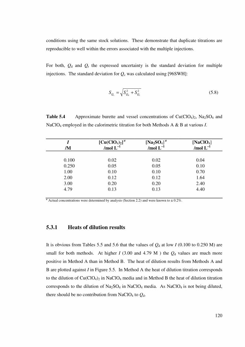
120
conditions using the same stock solutions. These demonstrate that duplicate titrations are
reproducible to well within the errors associated with the multiple injections.
For both, Qd and Qr the expressed uncertainty is the standard deviation for multiple
injections. The standard deviation for Qc was calculated using [96SWH]:
22
rdc QQQSSS += (5.8)
Table 5.4 Approximate burette and vessel concentrations of Cu(ClO4)2, Na2SO4 and
NaClO4 employed in the calorimetric titration for both Methods A & B at various I.
I [Cu(ClO4)2] a [Na2SO4]
a [NaClO4]
/M /mol L–1
/mol L–1
/mol L–1
0.100 0.02 0.02 0.04
0.250 0.05 0.05 0.10
1.00 0.10 0.10 0.70
2.00 0.12 0.12 1.64
3.00 0.20 0.20 2.40
4.79 0.13 0.13 4.40
a Actual concentrations were determined by analysis (Section 2.2) and were known to ± 0.2%.
5.3.1 Heats of dilution results
It is obvious from Tables 5.5 and 5.6 that the values of Qd at low I (0.100 to 0.250 M) are
small for both methods. At higher I (3.00 and 4.79 M ) the Qd values are much more
positive in Method A than in Method B. The heat of dilution results from Methods A and
B are plotted against I in Figure 5.5. In Method A the heat of dilution titration corresponds
to the dilution of Cu(ClO4)2 in NaClO4 media and in Method B the heat of dilution titration
corresponds to the dilution of Na2SO4 in NaClO4 media. As NaClO4 is not being diluted,
there should be no contribution from NaClO4 to Qd.
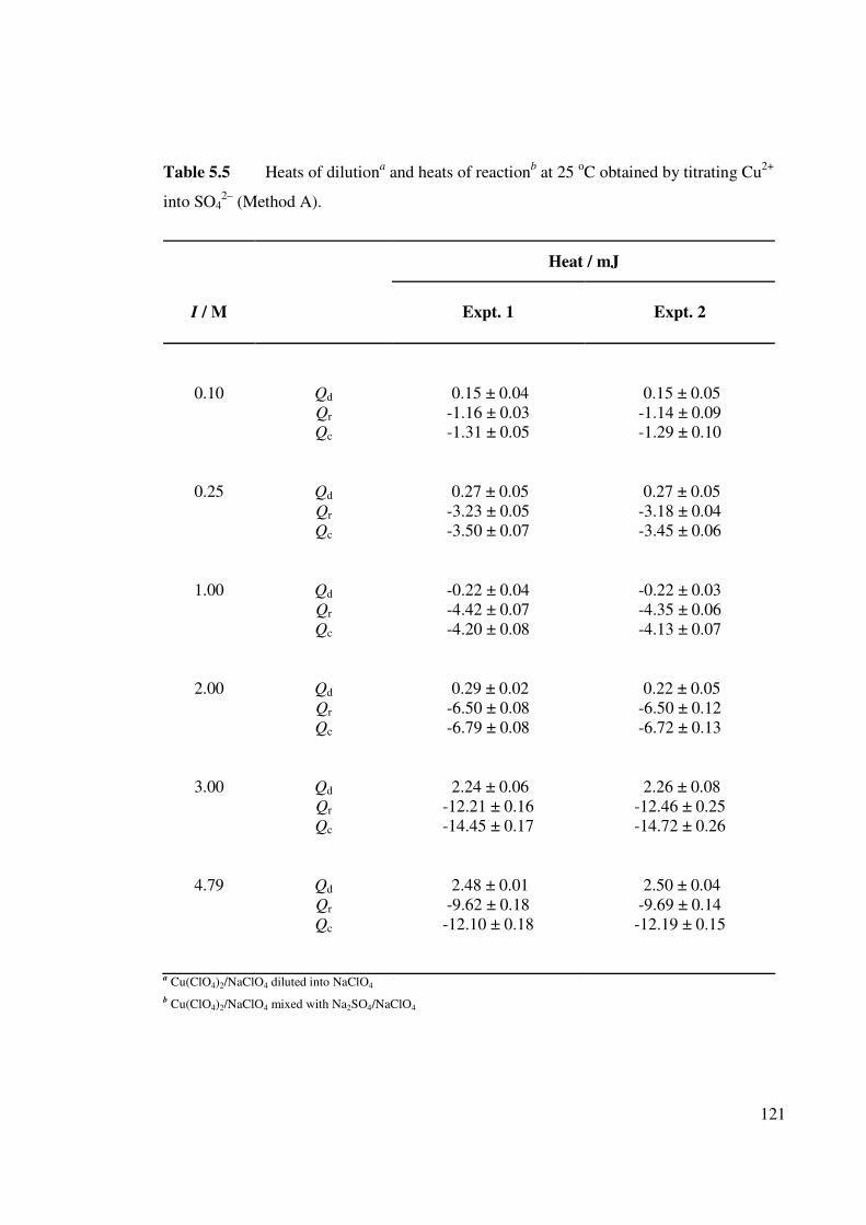
121
Table 5.5 Heats of dilutiona and heats of reaction
b at 25
oC obtained by titrating Cu
2+
into SO42–
(Method A).
Heat / mJ
I / M
Expt. 1 Expt. 2
0.10 Qd 0.15 ± 0.04 0.15 ± 0.05
Qr -1.16 ± 0.03 -1.14 ± 0.09
Qc -1.31 ± 0.05 -1.29 ± 0.10
0.25 Qd 0.27 ± 0.05 0.27 ± 0.05
Qr -3.23 ± 0.05 -3.18 ± 0.04
Qc -3.50 ± 0.07 -3.45 ± 0.06
1.00 Qd -0.22 ± 0.04 -0.22 ± 0.03
Qr -4.42 ± 0.07 -4.35 ± 0.06
Qc -4.20 ± 0.08 -4.13 ± 0.07
2.00 Qd 0.29 ± 0.02 0.22 ± 0.05
Qr -6.50 ± 0.08 -6.50 ± 0.12
Qc -6.79 ± 0.08 -6.72 ± 0.13
3.00 Qd 2.24 ± 0.06 2.26 ± 0.08
Qr -12.21 ± 0.16 -12.46 ± 0.25
Qc -14.45 ± 0.17 -14.72 ± 0.26
4.79 Qd 2.48 ± 0.01 2.50 ± 0.04
Qr -9.62 ± 0.18 -9.69 ± 0.14
Qc -12.10 ± 0.18 -12.19 ± 0.15
a Cu(ClO4)2/NaClO4 diluted into NaClO4
b Cu(ClO4)2/NaClO4 mixed with Na2SO4/NaClO4
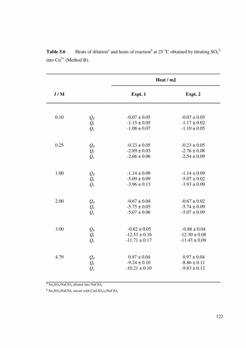
122
Table 5.6 Heats of dilutiona and heats of reaction
b at 25
oC obtained by titrating SO4
2-
into Cu2+
(Method B).
Heat / mJ
I / M
Expt. 1 Expt. 2
0.10 Qd -0.07 ± 0.05 -0.07 ± 0.05
Qr -1.15 ± 0.05 -1.17 ± 0.02
Qc -1.08 ± 0.07 -1.10 ± 0.05
0.25 Qd -0.23 ± 0.05 -0.23 ± 0.05
Qr -2.89 ± 0.03 -2.76 ± 0.08
Qc -2.66 ± 0.06 -2.54 ± 0.09
1.00 Qd -1.14 ± 0.09 -1.14 ± 0.09
Qr -5.09 ± 0.09 -5.07 ± 0.02
Qc -3.96 ± 0.13 -3.93 ± 0.09
2.00 Qd -0.67 ± 0.04 -0.67 ± 0.02
Qr -5.75 ± 0.05 -5.74 ± 0.09
Qc -5.07 ± 0.06 -5.07 ± 0.09
3.00 Qd -0.82 ± 0.05 -0.88 ± 0.04
Qr -12.53 ± 0.16 -12.30 ± 0.08
Qc -11.71 ± 0.17 -11.43 ± 0.09
4.79 Qd 0.97 ± 0.04 0.97 ± 0.04
Qr -9.24 ± 0.10 -8.86 ± 0.11
Qc -10.21 ± 0.10 -9.83 ± 0.12
a Na2SO4/NaClO4 diluted into NaClO4
b Na2SO4/NaClO4 mixed with Cu(ClO4)2/NaClO4
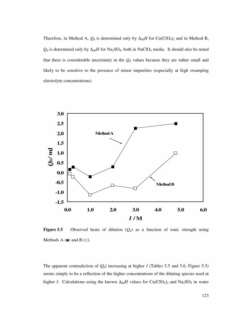
123
Therefore, in Method A, Qd is determined only by ∆dilH for Cu(ClO4)2 and in Method B,
Qd is determined only by ∆dilH for Na2SO4, both in NaClO4 media. It should also be noted
that there is considerable uncertainty in the Qd values because they are rather small and
likely to be sensitive to the presence of minor impurities (especially at high swamping
electrolyte concentrations).
-1.5
-1.0
-0.5
0.0
0.5
1.0
1.5
2.0
2.5
3.0
0.0 1.0 2.0 3.0 4.0 5.0 6.0
I / M
Qd / m
J
Method B
Method A
Figure 5.5 Observed heats of dilution (Qd) as a function of ionic strength using
Methods A () and B ().
The apparent contradiction of |Qd| increasing at higher I (Tables 5.5 and 5.6, Figure 5.5)
seems simply to be a reflection of the higher concentrations of the diluting species used at
higher I. Calculations using the known ∆dilH values for Cu(ClO4)2 and Na2SO4 in water
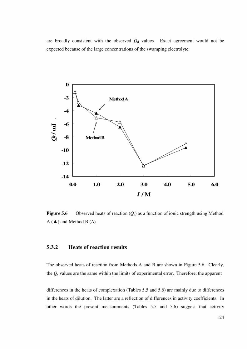
124
are broadly consistent with the observed Qd values. Exact agreement would not be
expected because of the large concentrations of the swamping electrolyte.
-14
-12
-10
-8
-6
-4
-2
0
0.0 1.0 2.0 3.0 4.0 5.0 6.0
I / M
Qr / m
J .
Method A
Method B
Figure 5.6 Observed heats of reaction (Qr) as a function of ionic strength using Method
A () and Method B (∆).
5.3.2 Heats of reaction results
The observed heats of reaction from Methods A and B are shown in Figure 5.6. Clearly,
the Qr values are the same within the limits of experimental error. Therefore, the apparent
differences in the heats of complexation (Tables 5.5 and 5.6) are mainly due to differences
in the heats of dilution. The latter are a reflection of differences in activity coefficients. In
other words the present measurements (Tables 5.5 and 5.6) suggest that activity
125
coefficients change significantly between a solution which is, say, (0.1 M Cu(ClO4)2 + 0.7
M NaClO4) and one which is (0.1 M Na2SO4 + 0.7 M NaClO4). Given the large
differences in the activity coefficients of the pure binary solutions of Cu(ClO4)2,
Na2SO4 (γ± = 0.452) and NaClO4 (γ± = 0.648) this is not surprising.
5.3.3 Enthalpy and entropy changes
Table 5.7 presents the enthalpies for the formation of 0
4CuSO from the free ions in NaClO4
media at 25 oC obtained using Methods A and B and their average. Also included are the
corresponding values of ∆G and ∆S (calculated from Equation 5.1). The uncertainty
assigned to the ∆H values is about 5% relative which does not include the uncertainty in
the KA values. The log KA (∆G) values were those determined in Chapter 3 by
potentiometry. The values of ∆H are endothermic and (Figure 5.7) show a similar trend to
log KA (Figure 2.7) against ionic strength.
The present results (Table 5.7) show that the precision in ∆H is worse at the lowest and
highest ionic strengths. Generally for this type of determination, the overall experimental
uncertainty consists of errors associated with measurement of Q and also the analytical
errors in [M]T and [L]T [66PVA]. Since the analytical error is more-or-less constant for a
given set of solutions most of the observed uncertainty must originate from the
measurement of the various Q values. The higher uncertainty at I = 0.1 M is therefore
most likely due to the concentrations of the reacting species (Cu2+
and SO42–
) not being
high enough to achieve a sufficiently large heat effect (Tables 5.5 and 5.6). At higher I,
where the uncertainty again increases this effect may possibly be due to trace impurities in
the supporting electrolyte producing spurious (small) heat effects.
Figure 5.7 presents the ∆H values for the formation of 0
4CuSO (aq) obtained via titration
Methods A and B together with the average values as a function of ionic strength. The
solid line calculated from Equation 5.9
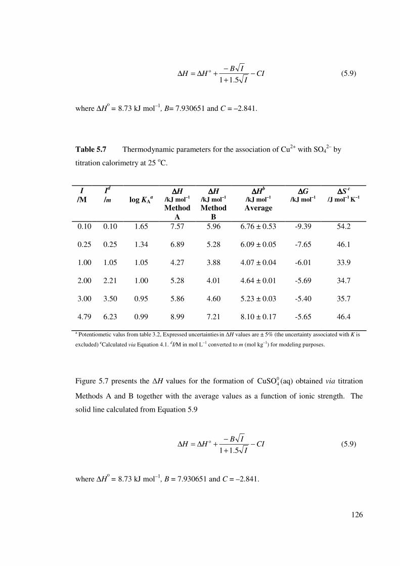
126
CII
IBHH −
+
−+ ∆=∆
5.11
o (5.9)
where ∆Ho = 8.73 kJ mol
–1, B= 7.930651 and C = –2.841.
Table 5.7 Thermodynamic parameters for the association of Cu2+
with SO42–
by
titration calorimetry at 25 oC.
I
/M
Id
/m
log KAa
∆∆∆∆H /kJ mol
–1
Method
A
∆∆∆∆H /kJ mol
–1
Method
B
∆∆∆∆Hb
/kJ mol–1
Average
∆∆∆∆G
/kJ mol–1
∆∆∆∆S c
/J mol–1
K–1
0.10 0.10 1.65 7.57 5.96 6.76 ± 0.53 -9.39 54.2
0.25 0.25 1.34 6.89 5.28 6.09 ± 0.05 -7.65 46.1
1.00 1.05 1.05 4.27 3.88 4.07 ± 0.04 -6.01 33.9
2.00 2.21 1.00 5.28 4.01 4.64 ± 0.01 -5.69 34.7
3.00 3.50 0.95 5.86 4.60 5.23 ± 0.03 -5.40 35.7
4.79 6.23 0.99 8.99 7.21 8.10 ± 0.17 -5.65 46.4
a Potentiometic valus from table 3.2, Expressed uncertainties in ∆H values are ± 5% (the uncertainty associated with K is
excluded) cCalculated via Equation 4.1. dI/M in mol L–1 converted to m (mol kg–1) for modeling purposes.
Figure 5.7 presents the ∆H values for the formation of 0
4CuSO (aq) obtained via titration
Methods A and B together with the average values as a function of ionic strength. The
solid line calculated from Equation 5.9
CII
IBHH −
+
−+ ∆=∆
5.11
o (5.9)
where ∆Ho = 8.73 kJ mol
–1, B = 7.930651 and C = –2.841.
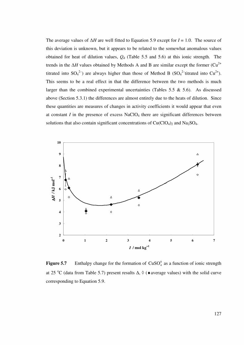
127
The average values of ∆H are well fitted to Equation 5.9 except for I = 1.0. The source of
this deviation is unknown, but it appears to be related to the somewhat anomalous values
obtained for heat of dilution values, Qd (Table 5.5 and 5.6) at this ionic strength. The
trends in the ∆H values obtained by Methods A and B are similar except the former (Cu2+
titrated into SO42–
) are always higher than those of Method B (SO42–
titrated into Cu2+
).
This seems to be a real effect in that the difference between the two methods is much
larger than the combined experimental uncertainties (Tables 5.5 & 5.6). As discussed
above (Section 5.3.1) the differences are almost entirely due to the heats of dilution. Since
these quantities are measures of changes in activity coefficients it would appear that even
at constant I in the presence of excess NaClO4 there are significant differences between
solutions that also contain significant concentrations of Cu(ClO4)2 and Na2SO4.
2
3
4
5
6
7
8
9
10
0 1 2 3 4 5 6 7
I / mol kg−−−−1
∆∆ ∆∆H
/ k
J m
ol−− −−
1
Figure 5.7 Enthalpy change for the formation of 0
4CuSO as a function of ionic strength
at 25 oC (data from Table 5.7) present results ∆, ◊ (♦average values) with the solid curve
corresponding to Equation 5.9.
128
The averaged results (Table 5.7) also show that the entropy change (∆S) decreases with
increasing I up to 2.0 M. The presence of the interacting ions (Cu2+
and SO42–
) may
disturb the solvent structure associated with the swamping electrolyte thereby lowering the
entropy term as I increases [77AH].
5.3.4 Standard enthalpy change (∆∆∆∆Ho) for 0
4CuSO (aq) formation
The standard (infinite dilution) enthalpy change ∆Ho for a reaction cannot be measured
directly but must be derived from experimental data obtained at finite concentrations at
low I by calculation or by the extrapolation of data measured at higher I using an
appropriate theoretical or semi-empirical expression. Models such as those of Masson
[79M, 02HMW], Pitzer [91P] or SIT [22B, 35G, 36S, 65G]) have been used for this
purpose.
Masson-type equations [79M] assume that the enthalpy change follows a simple square
root dependence on the ionic strength of the solution. In the case of the Cu2+
(aq)/SO42–
(aq)
system, it is obvious (Figure 5.7) that the enthalpy change does not depend simply on I
and thus use of a Masson-type equation will not give a reliable estimation of ∆Ho.
For enthalpies of reaction between ions, the SIT model can be expressed as [97GP],
IεRT
I
IzAHrLH
i
L
22
Lo
11.514
3∆−
+
∆×+∆=−∆ (5.10)
where r is the number of moles of water specifically participating in the reaction, L1 is the
relative partial molar enthalpy of water, AL is the Debye Hückel parameter for enthalpies
(at 25 oC and 1 atm, AL = 1.986 kJ kg
–1/2 mol
–3/2 ), ∆zi
2 is the change in the formal
charges of species involved in the reaction ((∆zi
2 = ∑z
2products - ∑z
2reactants) = –8) and
Lε∆ is
the change in the ion-interaction coefficients ( ( )ji
i
i,LL ενε ∑=∆ . Note that here the
129
subscript i refers to a reaction participant and j to the counter-ion of the ionic medium, and
the other terms have their usual meanings [97GP].
Equation 5.10 can also be written as,
IRTHrLIIAzHo
i L
2
1
1
L
2 )5.11(75.0 ε∆−∆=−+∆−∆− (5.11)
or, since water is not explicitly involved in the complex formation reaction, and therefore
r= 0:
IRTHIfHo
L
2
H )( ε∆−∆=−∆ (5.12)
where I
IzAIf
i
1.514
3)(
2
LH
+
∆×= represents the second term on the left hand side of Equation
5.11. Thus, a plot of )(H IfH −∆ vs. I should give a straight line with ∆Ho as the intercept.
Figure 5.7 shows the average ∆H values from this study (Table 5.7) fitted to the SIT
model. The intercept ∆Ho, has the value of 8.7 ± 0.5 kJ mol
–1 with ∆εL = 9.1×10
–4 kg
mol–1
K–1
.
Figure 5.8 shows that the present results are reasonably well fitted by the SIT model. The
experimental ∆H values at lower I lie above the SIT line. Such behaviour is often
observed when the SIT is used to model equilibria involving highly charged ions [07PBB].
This is probably a reflection of the variation of ∆εL with I and represents a real limitation
on the application of SIT model.
The result obtained from this study (8.7 ± 0.5 kJ mol–1
) is slightly higher than the average
∆Ho value for Cu
2+/SO4
2–system recommended by IUPAC [07PBB] (∆H
o = 7.3 ± 1.1 kJ
mol–1
) but is somewhat more precise and still agrees within the stated uncertainties.
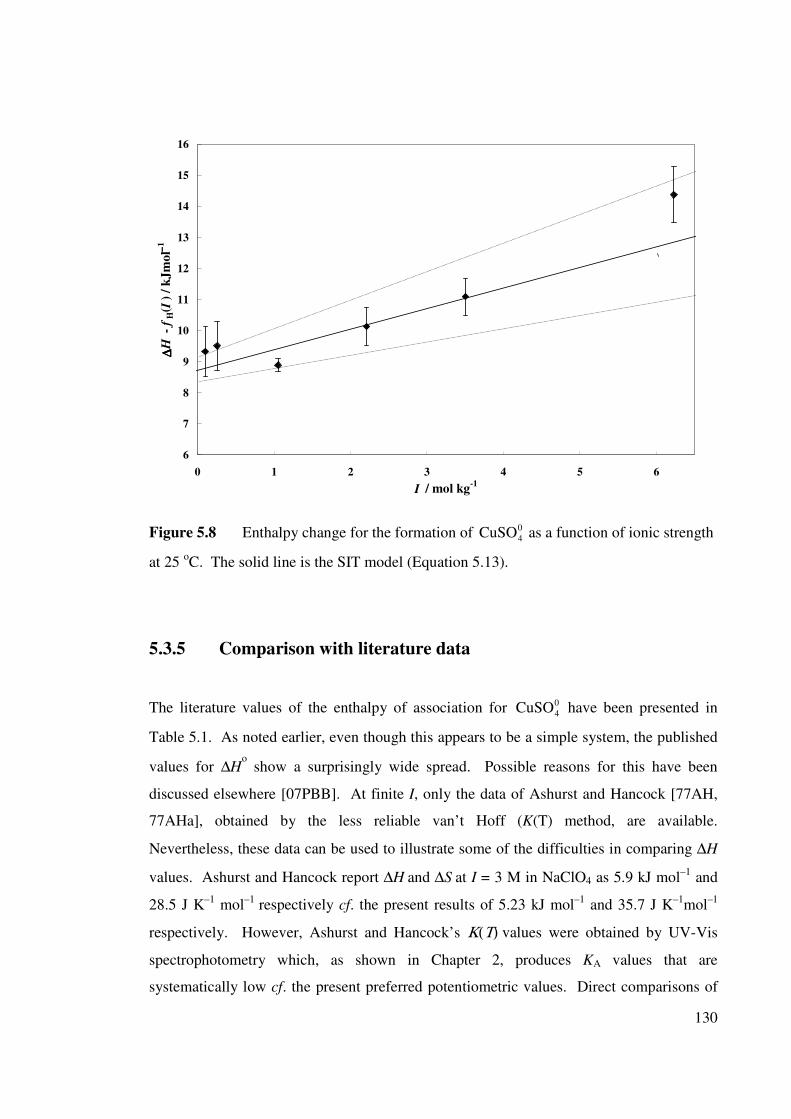
130
6
7
8
9
10
11
12
13
14
15
16
0 1 2 3 4 5 6
I / mol kg-1
∆∆ ∆∆H
- f
H( I
) /
kJ
mo
l−− −−1
Figure 5.8 Enthalpy change for the formation of 0
4CuSO as a function of ionic strength
at 25 oC. The solid line is the SIT model (Equation 5.13).
5.3.5 Comparison with literature data
The literature values of the enthalpy of association for 0
4CuSO have been presented in
Table 5.1. As noted earlier, even though this appears to be a simple system, the published
values for ∆Ho show a surprisingly wide spread. Possible reasons for this have been
discussed elsewhere [07PBB]. At finite I, only the data of Ashurst and Hancock [77AH,
77AHa], obtained by the less reliable van’t Hoff (K(T) method, are available.
Nevertheless, these data can be used to illustrate some of the difficulties in comparing ∆H
values. Ashurst and Hancock report ∆H and ∆S
at I = 3 M in NaClO4 as 5.9 kJ mol
–1 and
28.5 J K–1
mol–1
respectively cf. the present results of 5.23 kJ mol–1
and 35.7 J K–1
mol–1
respectively. However, Ashurst and Hancock’s Κ(Τ) values were obtained by UV-Vis
spectrophotometry which, as shown in Chapter 2, produces KA values that are
systematically low cf. the present preferred potentiometric values. Direct comparisons of
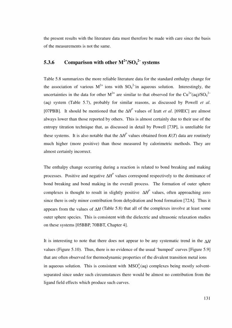
131
the present results with the literature data must therefore be made with care since the basis
of the measurements is not the same.
5.3.6 Comparison with other M2+
/SO42–
systems
Table 5.8 summarizes the more reliable literature data for the standard enthalpy change for
the association of various M2+
ions with SO42–
in aqueous solution. Interestingly, the
uncertainties in the data for other M2+
are similar to that observed for the Cu2+
(aq)/SO42–
(aq) system (Table 5.7), probably for similar reasons, as discussed by Powell et al.
[07PBB]. It should be mentioned that the ∆Ho values of Izatt et al. [69IEC] are almost
always lower than those reported by others. This is almost certainly due to their use of the
entropy titration technique that, as discussed in detail by Powell [73P], is unreliable for
these systems. It is also notable that the ∆Ho values obtained from K(T) data are routinely
much higher (more positive) than those measured by calorimetric methods. They are
almost certainly incorrect.
The enthalpy change occurring during a reaction is related to bond breaking and making
processes. Positive and negative ∆Ho values correspond respectively to the dominance of
bond breaking and bond making in the overall process. The formation of outer sphere
complexes is thought to result in slightly positive ∆Ho values, often approaching zero
since there is only minor contribution from dehydration and bond formation [72A]. Thus it
appears from the values of ∆H (Table 5.8) that all of the complexes involve at least some
outer sphere species. This is consistent with the dielectric and ultrasonic relaxation studies
on these systems [05BBP, 70BBT, Chapter 4].
It is interesting to note that there does not appear to be any systematic trend in the ∆H
values (Figure 5.10). Thus, there is no evidence of the usual ‘humped’ curves [Figure 5.9]
that are often observed for thermodynamic properties of the divalent transition metal ions
in aqueous solution. This is consistent with 0
4MSO (aq) complexes being mostly solvent-
separated since under such circumstances there would be almost no contribution from the
ligand field effects which produce such curves.
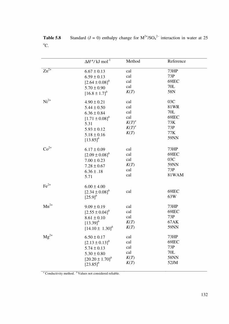
132
Table 5.8 Standard (I = 0) enthalpy change for M2+
/SO42–
interaction in water at 25
oC.
∆H° / kJ mol-1
Method Reference
Zn2+
6.67 ± 0.13
6.59 ± 0.13
[2.64 ± 0.08]b
5.70 ± 0.90
[16.8 ± 1.7]b
cal
cal
cal
cal
K(T)
73HP
73P
69IEC
70L
58N
Ni2+
4.90 ± 0.21
5.44 ± 0.50
6.36 ± 0.84
[1.71 ± 0.08]b
5.31
5.93 ± 0.12
5.18 ± 0.16
[13.85]b
cal
cal
cal
cal
K(T)a
K(T)a
K(T)
03C
81WR
70L
69IEC
73K
73P
77K
59NN
Co2+
6.17 ± 0.09
[2.09 ± 0.08]b
7.00 ± 0.23
7.28 ± 0.67
6.36 ± .18
5.71
cal
cal
cal
K(T)
cal
cal
73HP
69IEC
03C
59NN
73P
81WAM
Fe2+
6.00 ± 4.00
[2.34 ± 0.08]b
[25.9]b
cal
69IEC
63W
Mn2+
9.09 ± 0.19
[2.55 ± 0.04]b
8.61 ± 0.10
[13.39]b
[14.10 ± 1.30]b
cal
cal
cal
K(T)
K(T)
73HP
69IEC
73P
67AK
59NN
Mg2+
6.50 ± 0.17
[2.13 ± 0.13]b
5.74 ± 0.13
5.30 ± 0.80
[20.20 ± 1.70]b
[23.85]b
cal
cal
cal
cal
K(T)
K(T)
73HP
69IEC
73P
70L
58NN
52JM
a Conductivity method. b Values not considered reliable.
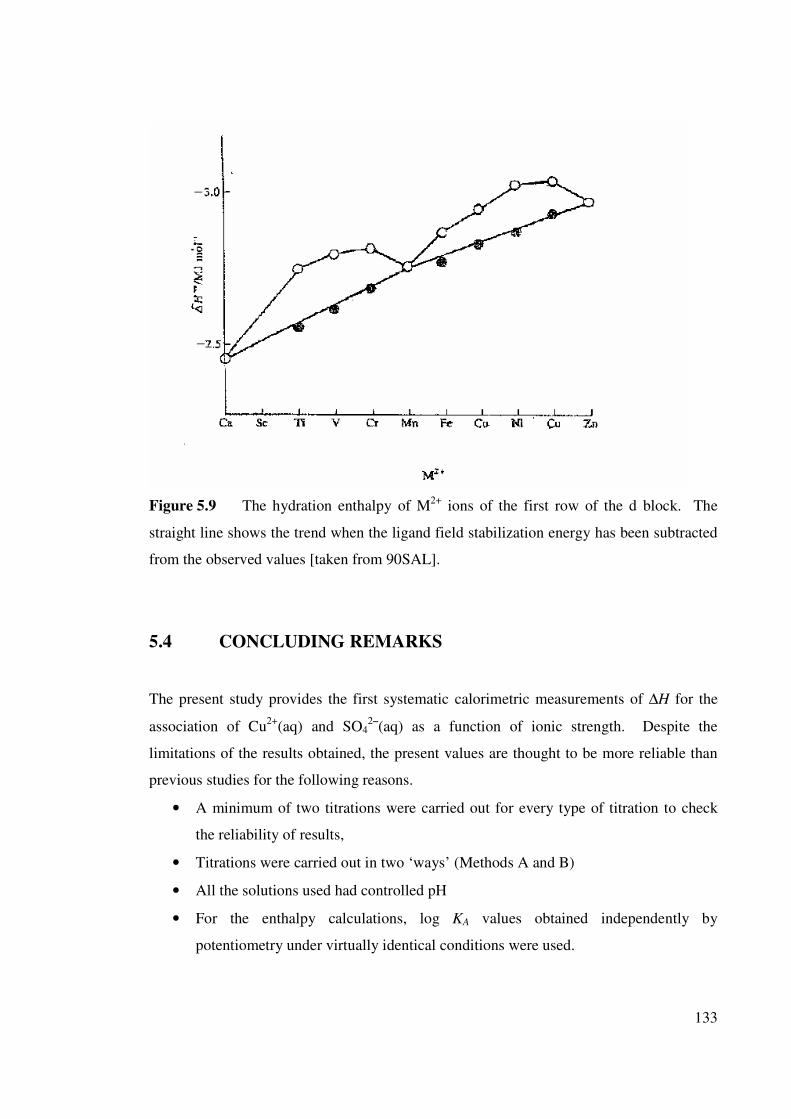
133
Figure 5.9 The hydration enthalpy of M2+
ions of the first row of the d block. The
straight line shows the trend when the ligand field stabilization energy has been subtracted
from the observed values [taken from 90SAL].
5.4 CONCLUDING REMARKS
The present study provides the first systematic calorimetric measurements of ∆H for the
association of Cu2+
(aq) and SO42–
(aq) as a function of ionic strength. Despite the
limitations of the results obtained, the present values are thought to be more reliable than
previous studies for the following reasons.
• A minimum of two titrations were carried out for every type of titration to check
the reliability of results,
• Titrations were carried out in two ‘ways’ (Methods A and B)
• All the solutions used had controlled pH
• For the enthalpy calculations, log KA values obtained independently by
potentiometry under virtually identical conditions were used.
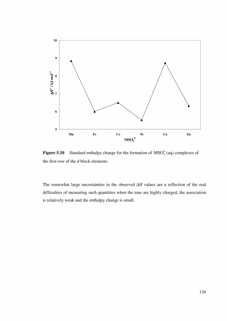
134
5
6
7
8
9
10
Mn Fe Co Ni Cu Zn
MSO40
∆∆ ∆∆H
o /
kJ
mo
l−− −−1
Figure 5.10 Standard enthalpy change for the formation of 0
4MSO (aq) complexes of
the first row of the d block elements.
The somewhat large uncertainties in the observed ∆H values are a reflection of the real
difficulties of measuring such quantities when the ions are highly charged, the association
is relatively weak and the enthalpy change is small.
135
Chapter Six
Physicochemical properties of binary and ternary
solutions of copper and related sulfates
6.1 BACKGROUND
6.1.1 Importance of physicochemical properties
The physicochemical properties of aqueous solutions of metal sulfates are of much interest
since they are components of many hydrometallurgical solutions, sea water, other natural
waters, and are also involved in acid mine drainage. As noted in Chapter 1, many of the
physicochemical properties of binary electrolyte solutions (consisting of one solute plus
the solvent) of interest to sulfate hydrometallurgy have been measured at 25 oC and
interpolative models have been established [68WRS]. However, the availability of
experimental physicochemical data for ternary aqueous sulfate solutions (solutions
consisting of two solutes plus the solvent) is limited and largely restricted to dilute or
moderately concentrated solutions [06D]. Studying the physicochemical properties of
ternary electrolytes at high concentrations is of great value for describing these properties
under industrially relevant conditions.
The osmotic coefficients, water activities and solute activity coefficients of aqueous
solutions of metal sulfate and mixtures are important for modeling reaction
thermodynamics, chemical speciation and solubilities [06D] and for understanding the
mechanism of reactions in sulfate hydrometallurgical systems [88MA]. Likewise,
densities are used in many practical situations such as chemical engineering designs for
areas such as power production from geothermal brines, oil well completion [70RC] and
hydrothermal processing of ores [93PAR, 06AZA] as well as being essential in the
development of solution theory and molecular thermodynamics [05WXZ]. Heat capacities
136
are essential for heat balance calculations in process engineering and for modeling any
process involving significant temperature changes. Heat capacities also provide important
insights into the microscopic properties of electrolyte solutions [77WH]. Solubilities are
important in a variety of industrial and environmental situations and in the recovery,
isolation, purification of many substances [85M, 02MKS]. Electrolyte solution viscosities
provide information on the nature of solutions [70RS, 95JM] but also are required for
engineering calculations relating to mass transfer, i.e. whenever such solutions must be
stirred, pumped or moved through pipes or other equipment [03HMS].
6.1.2 Selection of systems
As noted in Section 6.1.1, the physicochemical properties of aqueous electrolyte solutions
are of great technological importance. Not surprisingly therefore, the properties of binary
metal sulfate solutions have been studied fairly intensively over wide ranges of
concentration and temperature. However, relatively little is known about mixtures of salts.
This is significant because most industrial situations involve mixtures, which arise
inevitably when dealing with real substances. Accordingly, this chapter investigates key
physicochemical properties of a small range of mixtures of sulfate salts, namely, CuSO4,
MgSO4 and Na2SO4. These salts were selected because they are representative of the
sulfate salts found, for example, in the hydrometallurgical extraction and/or refinery of
copper, nickel and cobalt.
Published reports show that the osmotic coefficients of binary systems, Na2SO4 [70RS,
81RM, 00RCP], CuSO4 [70RS, 03GMD] and MgSO4 [70RS, 81RM, 98AR, 99HC,
03GMD] have been thoroughly studied at 25 oC. Several authors have also reported
measurements of osmotic coefficients or water activities of the ternary system Na2SO4-
MgSO4-H2O [68WRS, 81RM] at 25 oC. However, there are no published data available
for the Na2SO4-CuSO4-H2O and MgSO4-CuSO4-H2O systems. Densities of binary
solutions of Na2SO4 [66FKH, 80CCM, 97OMH, 02MKM], CuSO4 [37PP, 93PAR] and
MgSO4 [66FKH, 80CCM, 85I] are well characterized as too are the heat capacities
[92SLL, 02MKM]. However the densities and heat capacities of the ternary mixtures of
these solutions are scarce.
137
A wide range of solubility data of binary solutions involving Na2SO4 [41S, 65S, 91L,
99C], CuSO4 [19F, 26AB, 37MM] and MgSO4 [27K, 27R, 28RL, 29S, 34TM] solutions is
available in literature. Such solubilities have been extensively studied over a wide range of
conditions and some have also been measured in their ternary mixtures with H2SO4 and
other metal sulfates [24AG, 29S] at room temperature and other temperatures. However,
these studies were conducted several decades ago. Thus, the present investigation was
carried out to obtain the solubilities of CuSO4 and MgSO4 in Na2SO4 media at the
temperatures most relevant for industrial situations such as 60 and 90 oC and to compare
them with the literature values.
Electrolyte solution viscosities and their mixtures have been measured under various
conditions [68W, 72GP, 81KKC, 00SHM, 06AZA, 06AZAa, 06WMH]; however, the
present theoretical treatments still cannot accurately predict the behaviour of real systems.
There is therefore a requirement for more reliable viscosity data of electrolyte solutions
and their mixtures to develop better predictive models. Thus, viscosity measurements of
mixtures of CuSO4 solutions with Na2SO4 and MgSO4 were selected here with a view to
further understanding the properties of mixed solutions.
6.2 TECHNIQUES
6.2.1 Isopiestic method
The isopiestic method is a convenient, simple and popular method for determination of
osmotic coefficients, solvent activities and activity coefficients of electrolyte solutions.
This technique can be applied in principle to any solution comprising nonvolatile solutes
dissolved in a volatile solvent [79PR]. In this method, solutions are brought to equilibrium
by the transfer of solvent (alone) through the vapor phase. The equilibrium molalities of
the solutions can be determined accurately from the initial molalities of the solutions
together with the initial and final weights of the samples. Details of the isopiestic
technique are discussed at length in the review of Platford and Rard [79PR].
138
Isopiestic measurements are generally carried out by accurate weighing of samples of stock
solutions into appropriate vessels and then placing these in a sealed chamber. The
chamber (with or without evacuation) is positioned in a constant-temperature bath and is
left to equilibrate for an appropriate period of time, which may vary from several days to
many months depending on the particular apparatus, samples and conditions. At
equilibrium all the samples will have identical solvent activities (vapour pressure). The
sample vessels can then be removed from the chamber and weighed. The molalities at
isopiestic equilibrium can then be calculated using the known initial molalities and the
initial and the final weights of solution. Aqueous solutions of NaCl or KCl are generally
taken to be the reference standard, as the water activities of these solutions are known
accurately as a function of molality.
Isopiestic molality, m′ is calculated using the following equation [97HMM]
wwmM
mm
/)1000/1(1 1 ∆++=′ (6.1)
where m is the initial molality, w is the initial mass of the solution, w∆ is the mass change
of the solution and M1 is the molar mass of the involatile solute.
The osmotic coefficient of the sample solution can be calculated from the fundamental
equation for isopiestic equilibrium [97R]:
iimm ′∑= νφνφ /*** (6.2)
where ν*
and νi are the stoichiometric ionization numbers for the reference electrolyte and
the electrolyte i respectively (νi = 2 for NaCl(aq), MgSO4(aq) and CuSO4(aq) and νi = 3
for Na2SO4), m* and
im′ are the equilibrium molalities of the reference and sample
(unknown) solutions respectively, and *φ and φ are respectively the stoichiometric
molality-based osmotic coefficients of the reference solution and the mixed-electrolyte
solution i.e. ignoring any ion-pairing [97R].
139
6.2.2 Density
While densities of electrolyte solutions have been measured by pycnometry as early as the
1800s, most modern density measurements use vibrating tube techniques [02G, 04LC].
The principle of a vibrating-tube density meter is that, the difference )( ρ∆ between the
density of an electrolyte solution, ρ, and that of the pure solvent, ρo, in such a tube is
related to the change in the square of the natural vibration period of the tube 2τ [79P]:
22
o
2
o )( τττρρρ ∆=−=−=∆ KK (6.3)
where K is a (mechanical) constant of the vibrating tube, which is constant for a particular
tube at constant temperature and pressure. The value of K is determined by measuring the
τ values of two reference solutions of accurately known densities under the desired
conditions. In this study, high purity degassed water (ρo = 0.997047 g cm–3
) and dry air (ρ
= 0.001185 g cm–3
) [88WAB] were used.
Apparent molal volumes
Experimentally-measured densities can be used to calculate apparent molal volumes φ
V of
binary electrolyte solutions using the following equation [71M, 71Ma].
m
MV
o
oφ
)(1000
ρρ
ρρ
ρ
−−= (6.4)
where m is the molality of the solution in mol kg–1
and M is the molar mass of the
electrolyte in g mol–1
and the densities are in g cm–3
.
For ternary mixtures of two salts (2 & 3) in solution, the apparent molal volumes φ
V (2,3)
were calculated from
140
To
oTφ
)(1000)3,2(
m
MV
ρρ
ρρ
ρ
−−= (6.5)
where Tm is the total molality of the mixture ( Tm = m2 + m3), and MT is the average molar
mass of the mixture (MT = M2Y2 + M3Y3, where M2 and M3 are molar masses of electrolytes
2 and 3 respectively. Yi is taken as mi/mT). According to Young’s rule [54YS], the
apparent molal volume of the ternary mixture can also be calculated using
32
3φ32φ2
φ)3,2(
nn
VnVnV
+
+= (6.6)
where 2φV and 3φV are the apparent molal volumes of electrolytes 2 and 3 in their binary
solutions whose ionic strength is that of the ternary mixture.
6.2.3 Heat capacity
Flow calorimeters have revolutionalized the measurement of heat capacities of fluids
because of their sensitivity, precision and speed [96HH]. Although some doubts were
raised about their accuracy because of possible heat losses [76DVP, 76FBP] these
problems seem to have mostly been overcome in most recent instruments. The calorimeter
is capable of measuring directly the difference in the isobaric volumetric heat capacity of
two liquids flowing sequentially, in a continuous column, through a reference and a
working cell [71PLP, 02MKM]. When the test solution is in the working cell and the
reference liquid is in the reference cell, the relative volumetric heat capacity difference
between two liquids can be calculated [76DVP, 02MKM],
o
1
o
o
o
)(
W
W∆=
−=
∆
σ
σσ
σ
σ (6.7)
where oσ is the isobaric heat capacity per unit volume of the reference liquid,
oW is
the
baseline power applied to the cells and 1W∆ is the difference in the applied power
necessary to maintain the temperature of both liquids exactly equal.
141
When the test solution is in the reference cell and the reference liquid is in the working
cell, Equation 6.7 [76DVP] can be written as,
)( 2o
2
o WW
W
∆+
∆−=
∆
σ
σ (6.8)
where ∆W2 is the extra power applied to maintain the reference liquid at the same ‘final’
temperature as that of the test solution [02MKM].
The isobaric heat capacities per unit mass pc (J K
–1g
–1) of the solution were calculated
from the volumetric heat capacities using the expression [76DVP]
ρσσρ /)/1( oo
o
pp ∆+= cc (6.9)
where o
pc is the heat capacity of the reference liquid (water), which was taken as 4.1819 J
g–1
K–1
[02MKM] and oρ is the density of the reference liquid. For binary solutions, the
apparent molar heat capacities, pφC (J K–1
mol–1
) were calculated from the expression
]/)(1000[ o
ppppφ mccMcC −+= (6.10)
The mean apparent molar heat capacities of the ternary mixtures pφC (2,3) were calculated
from the expression [02MKM]
)/(]1000)1000([)3,2( 32
o
p3322ppφ mmcMmMmcC +−++= (6.11)
where the subscripts 2 and 3 refer to the two solutes. Apparent molar heat capacities of
ternary mixtures can also be calculated using Young’s rule [88HHT]
3pφ32pφ2pφ )/()/()3,2( CImCImC += (6.12)
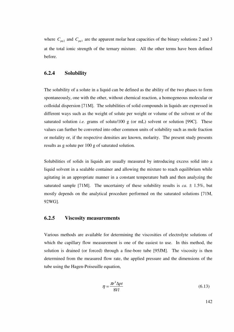
142
where 2pφC and 3pφC are the apparent molar heat capacities of the binary solutions 2 and 3
at the total ionic strength of the ternary mixture. All the other terms have been defined
before.
6.2.4 Solubility
The solubility of a solute in a liquid can be defined as the ability of the two phases to form
spontaneously, one with the other, without chemical reaction, a homogeneous molecular or
colloidal dispersion [71M]. The solubilities of solid compounds in liquids are expressed in
different ways such as the weight of solute per weight or volume of the solvent or of the
saturated solution i.e. grams of solute/100 g (or mL) solvent or solution [99C]. These
values can further be converted into other common units of solubility such as mole fraction
or molality or, if the respective densities are known, molarity. The present study presents
results as g solute per 100 g of saturated solution.
Solubilities of solids in liquids are usually measured by introducing excess solid into a
liquid solvent in a sealable container and allowing the mixture to reach equilibrium while
agitating in an appropriate manner in a constant temperature bath and then analyzing the
saturated sample [71M]. The uncertainty of these solubility results is ca. ± 1.5%, but
mostly depends on the analytical procedure performed on the saturated solutions [71M,
92WG].
6.2.5 Viscosity measurements
Various methods are available for determining the viscosities of electrolyte solutions of
which the capillary flow measurement is one of the easiest to use. In this method, the
solution is drained (or forced) through a fine-bore tube [95JM]. The viscosity is then
determined from the measured flow rate, the applied pressure and the dimensions of the
tube using the Hagen-Poiseuille equation,
Vl
ptr
8
4∆
=π
η (6.13)
143
where r is the radius of the constant-bore capillary, l is its length, ∆p is the pressure drop
along the capillary, V is the volume of liquid that flows during time t.
Various theories and equations have been introduced to explain the changes in viscosity of
a solution with its concentration. The Falkenhagen-Dole equation describes the relative
viscosities of a binary electrolyte solution at low concentrations (c < ca. 0.05 M) [06AZA].
cA+= 1oηη (6.14)
where η and oη are the dynamic viscosity of the solution and the pure solvent respectively,
the constant A is a function of solvent properties, ionic charges and mobilities respectively,
and temperature [70RS]. The semi-empirical Jones-Dole equation is used to correlate the
relative viscosities of electrolyte solutions with moderate concentrations (c < ca. 0.5 M).
BccAo
++= 1ηη (6.15)
where the empirical parameter B is known as ‘Jones-Dole B-coefficient’ [95JM, 03HMS].
Rearranging Equation 6.15 gives
2/12/1
o /)1( BcAc +=−ηη (6.16)
and the value of the coefficient A can be obtained either from the intercept of a plot of
2/1/)1/( co
−ηη against 2/1c or calculated theoretically if the equivalent conductivities of
the ions in the solution are known [95JM, 06AZA]. The B coefficient is a useful quantity
as it provides information concerning the solvation of the ions and their effects on the
solvent structure [95JM, 06AZA] and is readily obtained from the slope of the plot
2/1/)1/( c
o−ηη against 2/1
c .
144
Various empirical extensions to the Jones-Dole equation have been proposed [33JT, 57K,
72DP] to correlate viscosities of electrolyte solutions with higher concentrations (> 0.5 M).
For example:
BccAo
++= 1ηη +Dc2 (6.17)
The extra empirical term Dc2 includes all solute-solvent and solute-solute structural
interactions that were not accounted for by cA and Bc terms at higher concentrations
[06AZA].
6.3 EXPERIMENTAL
6.3.1 Isopiestic measurements
The isopiestic measurements were performed using an isopiestic apparatus [97HMM]
based on the design of Grjotheim et al. [88GVH] that contains stainless-steel cups, a gold-
plated copper block and an evacuable stainless steel chamber. A detailed description of
this apparatus is given by Hefter et al. [97HMM]. The present measurements were
performed as three series of experiments for aqueous mixtures of Na2SO4/CuSO4,
Na2SO4/MgSO4 and CuSO4/MgSO4 at 25 oC using NaCl(aq) as the isopiestic reference
standard in all cases.
Stock solutions of ~1 mol/kg of NaCl(aq) (99.5%, BDH, AnalaR), Na2SO4, (99%, APS
fine Chem., Univar), CuSO4.5H20 (98%, BioLab, proanlys AR) and MgSO4 (99% BDH,
AnalaR) were prepared using oven-dried salts without further purification. Concentrations
of aqueous CuSO4 and MgSO4 stock solutions were obtained to ± 0.2% by complexometric
titration with standard EDTA solution (BDH, UK, concentrated volumetric standard). The
isopiestic samples of mixed solutions were prepared by weight from these stock solutions
keeping the ratio of 1:4, 2:3, 3:2, 4:1 and 1:1 either as Na2SO4/CuSO4, or Na2SO4/MgSO4
or CuSO4/MgSO4.
145
Duplicate samples of the isopiestic reference standard, NaCl(aq), and binary solutions of
Na2SO4, CuSO4, and/or MgSO4, were equilibrated together with ternary solutions of
Na2SO4-CuSO4-H2O or Na2SO4-MgSO4-H2O or CuSO4-MgSO4-H2O in each experiment.
Each experiment was left for 7 – 8 weeks for the solutions to equilibrate. The osmotic
coefficients for the reference standards, *φ for NaCl(aq) were obtained from the Bayer.exe
computer program [05KEM].
6.3.2 Density measurements
Densities were measured at 25 oC using an Anton Paar DMA 602 vibrating tube density
meter connected to an Anton Paar mPDS 400 data module that measured the period of
vibration of the tube (τ). A Julabo F-33 heating and refrigerating circulator-thermostat
provided temperature control within ± 0.02 K. Some measurements were also made with
an Anton Paar Precision density meter (DMA 02D) at 25 ± 0.01 oC, controlled by a Haake
K-20 circulator.
The salts required for preparing the necessary solutions were the same as those described
previously (Chapter 2, Section 2.2). Binary solutions of Na2SO4, CuSO4, MgSO4 and the
ternary mixture Na2SO4-CuSO4-H2O at I = 1.00 mol kg–1
were prepared by weight using
the appropriate salt and high purity (Milli Q) water and filtered (0.45 µm) under vacuum
and degassed.
Apparent molal volumes of binary and ternary mixtures were calculated using the
measured densities of solutions and Equations 6.4 and 6.5.
6.3.3 Heat capacity measurements
Heat capacities were determined with a Picker flow microcalorimeter (Sodev, Model CP-
C) [71PLP]. The temperature was controlled by a Sodev circulator-thermostat (Model CT-
L). Test solutions and the reference solutions were introduced into the calorimeter through
a four way chromatography valve (Hamilton, U.S.A., model HVP). The flow rate was
maintained at 0.6 cm3 min
–1 by a peristaltic pump (Gilson, Minipuls 3) [02MKM]. The
146
voltage output from the calorimeter detector was monitored with an integrating voltmeter
(Hewlett-Packard, model 34401A) for period from 30 to 60 s. The details of this
instrument, its temperature control and the calculations involved have been described
elsewhere [71PLP, 02MKM, 03C, 05TKM].
Binary solutions of Na2SO4, CuSO4, MgSO4 and the ternary mixtures Na2SO4-CuSO4-H2O
at I = 1.00 mol kg–1
were prepared by weight using the appropriate salts and high purity
(Milli Q) water and filtered (0.45 µm) under vacuum and degassed. All the salts used in
these stock solutions were described previously (Section 2.2).
6.3.4 Solubility measurements
A solubility apparatus developed at Murdoch University [99CHM] was used for this study.
This apparatus allows the solid/liquid mixture to equilibrate in a temperature-controlled
water bath while providing continuous gentle mixing of the solute and solution. This
apparatus allows sampling of the liquid phase without the need to remove the sample from
its environment. The apparatus and the equilibration vessels and sampling procedure have
been described in greater detail elsewhere [99C, 03T].
An appropriate amount of the solid (CuSO4 or MgSO4) was added to the solution (Na2SO4)
contained in disposable polypropylene Luer-lock syringes (50 mL, Aldrich Australia) such
that the solutions were ca. 90% saturated with respect to the solid. Excess solid was then
added to the syringes, which were capped and fitted on a carousel in a constant temperature
water bath. The samples were allowed to equilibrate for about two weeks. After
equilibration, the syringes to be sampled were transferred one by one (without removal
from the bath) from the carousel to the sampling device. Duplicate aliquots of the
saturated solutions were then forced from the syringes through a 0.45µm filter as described
in detail elsewhere [99C]. Saturated solutions were analyzed using complexometric
titration with standard EDTA [89JBM].
The salts selected for this study, CuSO4·5H2O, (Ajax, Australia, 98 - 102%) and
MgSO4·7H2O, (Biolab Pronalys AR 98% ) were used without further purification. Four
147
stock solutions of Na2SO4 of accurately known concentrations (1) 0.3505, (2) 0.6866,
(3) 1.0292 and (4) 1.3819 mol kg–1
were prepared by weight using required amount of salt
and high purity (Milli Q) water.
6.3.5 Viscosity measurements
Viscosities were measured using a conventional Ubbelohde glass capillary flow viscometer
system (Schott-Geräte type 53003 with capillary numbers 0a and 0c and capacity 15 – 20
mL). The viscometer tube was held in an AVS/S measuring stand fitted with two
phototransistors and detectors [00SHM]. This system was connected to a Schott-Geräte
AVS 310 measuring system with automatic recording flow times to ± 0.01 s [00SHM,
01SSB]. The viscometer and the measuring stand were kept in a transparent continuously
stirred water bath. The temperature of the system was maintained at 25.0 ± 0.005 oC with
locally constructed regulator unit [00SHM] and was continuously monitored with Hewlett-
Packard quartz crystal thermometer. Further details of the water bath and the temperature
control system are given elsewhere [00SHM, 01SSB]. The apparatus was kept in a room
with controlled temperature at 20 ± 2 oC.
The viscometer capillaries were cleaned thoroughly with high purity water, oven dried and
then rinsed three times with the test solution before filling. Further details for cleaning and
filling the viscometers are given in the operating manual [08A]. The filled viscometer was
placed in a vertical position in the constant temperature (25.00 ± 0.005 oC) water bath.
After thermal stability was attained, the efflux times of the test solutions were measured
for duplicate fillings, each measured ten times with the automatic measuring unit. The
measurements were accepted when replicates reproduced to ± 0.05 s.
The kinematic viscosity, ν (mm2/s) is calculated using
)( θν −= tK (6.18)
where K is a constant specific for each capillary at constant temperature and pressure, t is
the average flow time, θ is the flow-time-dependent empirical (Hagenbach) correction
148
factor provided by the viscometer manufacturer [08A]. The K value can be obtained by
calibrating the viscometer with a reference liquid of accurately known viscosity.
However, the dynamic viscosity of a solution can be obtained directly without calculating
the K value. Given that kinematic viscosity of the reference liquid, oν is
)( ooo θν −= tK (6.19)
and that the densities of water and the sample are oρ and ρ respectively, the dynamic
viscosity η can be calculated as follows. From Equations 6.18, and 6.19, the dynamic
viscosities of the reference and the sample are respectively given by,
ρθνρη )( −== tK (6.20)
ooooo )( ρθρνη −== tKo
(6.21)
Dividing Equation 6.20 by 6.21 gives
oooo )(
)(
ρθ
ρθ
η
η
−
−=
t
t (6.22)
or
ooo
o)(
)(
ρθ
ρθηη
−
−=
t
t (6.23)
The viscometer was calibrated with degassed and filtered (0.45 µm) high purity water and
tested using standard NaCl solutions before introducing the samples. The density and
dynamic viscosity of water were taken to be 0.997047 g cm–3
and 0.8901 mPa s [81JER]
respectively. The kinematic viscosity of 1.000 mol kg–1
NaCl(aq) obtained from this study
(0.9388 mm2 s
–1) is in excellent agreement with the reference value of 0.9380 mm
2 s
–1
[81KKC]. Viscosities of the samples were measured in duplicates using two different
capillaries (0a and 0c). As densities of the samples were required for the calculation of
dynamic viscosity, they were also measured as described in Section 6.3.2.
149
Aqueous ∼1 mol kg–1
stock solutions of Na2SO4, MgSO4 and CuSO4 were prepared
individually from analytical grade reagents, similar to those used before (Section 6.3.1)
and analysed by the procedures described in Section 6.3.1.
Solution series at a constant ionic strength of 3 mol kg–1
(Na2SO4+MgSO4), 3 mol kg–1
(Na2SO4+CuSO4) and 4 mol kg–1
(MgSO4+CuSO4) consisting of 21 individual samples of
~100 mL total volume were prepared by weighing appropriate (Na2SO4/MgSO4),
(Na2SO4/CuSO4) and (MgSO4/CuSO4) stock solutions. Although every attempt was taken
to obtain similar concentrations in each constituent of solution, slightly different
concentrations in each set of experiments was unavoidable. Buoyancy corrections were
not applied during solution preparation so the overall accuracy of the concentrations is not
better than 0.1% relative [00SHM].
6.4 ISOPIESTIC MOLALITIES AND OSMOTIC
COEFFICIENTS RESULTS
Calculated isopiestic molalities and osmotic coefficients of the binary solutions and their
mixtures are listed in Table 6.1 along with their uncertainties. The uncertainties are based
on the agreement between the molalities of the duplicate samples. The long equilibration
times (7 – 8 weeks) used in the present study contributes to the good precision of the
isopiestic molalities and osmotic coefficients of Na2SO4(aq), CuSO4(aq) and MgSO4(aq).
The present osmotic coefficient data for the binary solutions of Na2SO4, CuSO4 and
MgSO4 are compared with literature data [70RS, 81RM, 03GMD] in Figure 6.1. These
results are all in reasonably good agreement. The average deviation without regard to sign
between the present osmotic coefficients and those given by Robinson and Stokes [70RS]
were: Na2SO4, 0.008, CuSO4, 0.009 and MgSO4, 0.010.
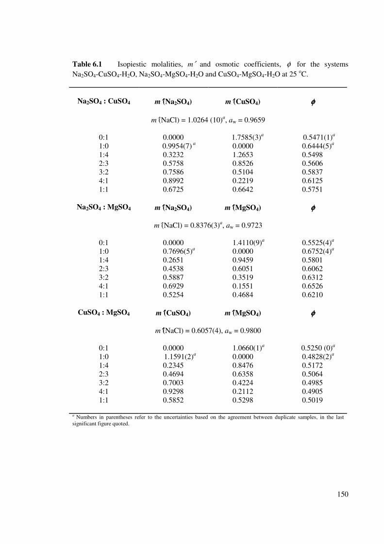
150
Table 6.1 Isopiestic molalities, m′ and osmotic coefficients, φ for the systems
Na2SO4-CuSO4-H2O, Na2SO4-MgSO4-H2O and CuSO4-MgSO4-H2O at 25 oC.
Na2SO4 : CuSO4 m′′′′(Na2SO4) m′′′′(CuSO4) φφφφ
m′(NaCl) = 1.0264 (10)a, aw = 0.9659
0:1 0.0000 1.7585(3)a 0.5471(1)
a
1:0 0.9954(7) a
0.0000 0.6444(5)a
1:4 0.3232 1.2653 0.5498
2:3 0.5758 0.8526 0.5606
3:2 0.7586 0.5104 0.5837
4:1 0.8992 0.2219 0.6125
1:1 0.6725 0.6642 0.5751
Na2SO4 : MgSO4 m′′′′(Na2SO4) m′′′′(MgSO4) φφφφ
m′(NaCl) = 0.8376(3)a, aw = 0.9723
0:1 0.0000 1.4110(9)a 0.5525(4)
a
1:0 0.7696(5)a 0.0000 0.6752(4)
a
1:4 0.2651 0.9459 0.5801
2:3 0.4538 0.6051 0.6062
3:2 0.5887 0.3519 0.6312
4:1 0.6929 0.1551 0.6526
1:1 0.5254 0.4684 0.6210
CuSO4 : MgSO4 m′′′′(CuSO4) m′′′′(MgSO4) φφφφ
m′′′′(NaCl) = 0.6057(4), aw = 0.9800
0:1 0.0000 1.0660(1)a 0.5250 (0)
a
1:0 1.1591(2)a 0.0000 0.4828(2)
a
1:4 0.2345 0.8476 0.5172
2:3 0.4694 0.6358 0.5064
3:2 0.7003 0.4224 0.4985
4:1 0.9298 0.2112 0.4905
1:1 0.5852 0.5298 0.5019
a Numbers in parentheses refer to the uncertainties based on the agreement between duplicate samples, in the last
significant figure quoted.

151
Figure 6.1 Osmotic coefficient data for binary solutions of Na2SO4, MgSO4 and CuSO4
at 25 oC. (Na2SO4: [70RS], [03GMD], Present Study; MgSO4: [70RS], X
[81RM], • Present Study; CuSO4: ∆ [70RS], + [03GMD] Present Study).
0.40
0.45
0.50
0.55
0.60
0.65
0.70
0.75
0.80
0.85
0.90
0.0 1.0 2.0 3.0 4.0
m (MSO4)/ mol kg-1
φ φ φ φ
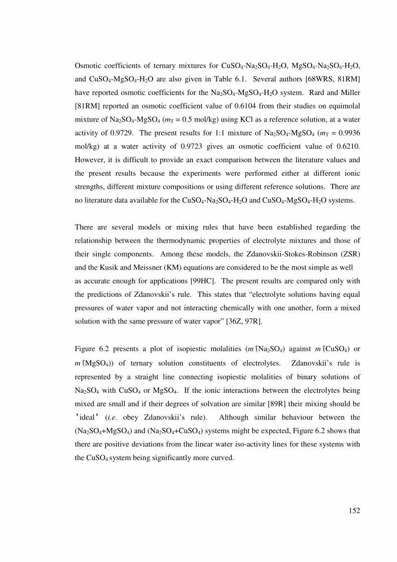
152
Osmotic coefficients of ternary mixtures for CuSO4-Na2SO4-H2O, MgSO4-Na2SO4-H2O,
and CuSO4-MgSO4-H2O are also given in Table 6.1. Several authors [68WRS, 81RM]
have reported osmotic coefficients for the Na2SO4-MgSO4-H2O system. Rard and Miller
[81RM] reported an osmotic coefficient value of 0.6104 from their studies on equimolal
mixture of Na2SO4-MgSO4 (mT = 0.5 mol/kg) using KCl as a reference solution, at a water
activity of 0.9729. The present results for 1:1 mixture of Na2SO4-MgSO4 (mT = 0.9936
mol/kg) at a water activity of 0.9723 gives an osmotic coefficient value of 0.6210.
However, it is difficult to provide an exact comparison between the literature values and
the present results because the experiments were performed either at different ionic
strengths, different mixture compositions or using different reference solutions. There are
no literature data available for the CuSO4-Na2SO4-H2O and CuSO4-MgSO4-H2O systems.
There are several models or mixing rules that have been established regarding the
relationship between the thermodynamic properties of electrolyte mixtures and those of
their single components. Among these models, the Zdanovskii-Stokes-Robinson (ZSR)
and the Kusik and Meissner (KM) equations are considered to be the most simple as well
as accurate enough for applications [99HC]. The present results are compared only with
the predictions of Zdanovskii’s rule. This states that “electrolyte solutions having equal
pressures of water vapor and not interacting chemically with one another, form a mixed
solution with the same pressure of water vapor” [36Z, 97R].
Figure 6.2 presents a plot of isopiestic molalities (m′(Na2SO4) against m′(CuSO4) or
m′(MgSO4)) of ternary solution constituents of electrolytes. Zdanovskii’s rule is
represented by a straight line connecting isopiestic molalities of binary solutions of
Na2SO4 with CuSO4 or MgSO4. If the ionic interactions between the electrolytes being
mixed are small and if their degrees of solvation are similar [89R] their mixing should be
'ideal' (i.e. obey Zdanovskii’s rule). Although similar behaviour between the
(Na2SO4+MgSO4) and (Na2SO4+CuSO4) systems might be expected, Figure 6.2 shows that
there are positive deviations from the linear water iso-activity lines for these systems with
the CuSO4 system being significantly more curved.
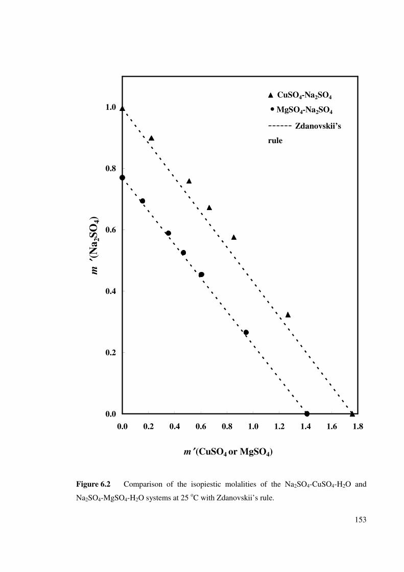
153
0.0
0.2
0.4
0.6
0.8
1.0
0.0 0.2 0.4 0.6 0.8 1.0 1.2 1.4 1.6 1.8
m ′′′′(CuSO4 or MgSO4)
m ′′ ′′
(Na
2S
O4)
CuSO4-Na2SO4
• MgSO4-Na2SO4
------ Zdanovskii’s
rule
Figure 6.2 Comparison of the isopiestic molalities of the Na2SO4-CuSO4-H2O and
Na2SO4-MgSO4-H2O systems at 25 oC with Zdanovskii’s rule.
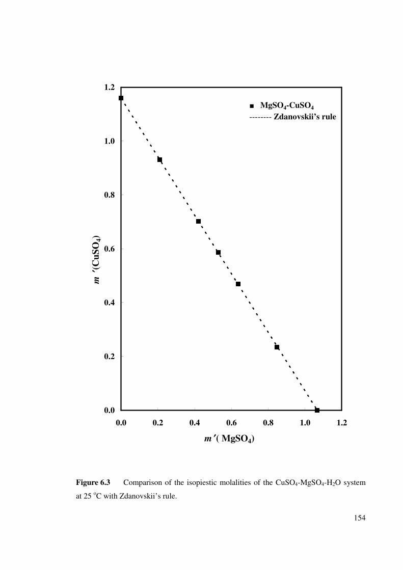
154
0.0
0.2
0.4
0.6
0.8
1.0
1.2
0.0 0.2 0.4 0.6 0.8 1.0 1.2
m ′′′′( MgSO4)
m ′′ ′′
(Cu
SO
4)
MgSO4-CuSO4
-------- Zdanovskii’s rule
Figure 6.3 Comparison of the isopiestic molalities of the CuSO4-MgSO4-H2O system
at 25 oC with Zdanovskii’s rule.
155
In other words, (Na2SO4+CuSO4) shows greater departures from Zdanovskii’s rule than
does (Na2SO4+MgSO4). The plot (Figure 6.3) of the isopiestic molalities (m′(CuSO4) and
m′(MgSO4)) of the ternary system CuSO4-MgSO4-H2O shows that it closely follows the
water iso-activity line for the system. This is perhaps not surprising given that this system
contains a common anion, SO42–
, and that the mixing is occuring between 2:2 electrolytes
and that this interactions between Mg2+
and Cu2+
with SO42–
are known to be very similar.
6.5 DENSITY RESULTS
As stated earlier (Chapter 1, Section 1.7) density measurements at 25 oC of binary aqueous
solutions of electrolytes such as Na2SO4 [22T, 27G, 35L, 52E, 68KF, 86PP, 02MKM],
CuSO4, [14H, 16HP, 19HP, 37PP, 73P, 93PAR] and MgSO4 [52E, 57K, 68KF, 73MK,
80CCM, 85I, 86PP] are abundant in the literature. Although, those measurements were
carried out at 25 oC as is the present study, densities of Na2SO4, CuSO4 and MgSO4
solutions were studied again for comparison before considering the ternary mixtures. The
densities and heat capacities of Na2SO4, CuSO4 and MgSO4 are summarized in Tables 6.2
along with the corresponding apparent molal volumes and apparent molar heat capacities.
The reproducibility of the density measurements was better than ± 10 µg cm–3
.
The performance of the density meter was assessed with standard NaCl solutions (1.000
and 2.000 mol kg–1
) and the results (1.036128 and 1.072268 g cm–1
respectively) are in
good agreement with literature data [03T] (1.036181 and 1.072216 g cm–1
), [80I] (1.03607
g cm–1
) and [02MKM] (1.072270 g cm–1
) respectively. The densities of Na2SO4 are also in
good agreement with Magalhães et al. [02MKM] and those of Korosi and Fabuss [68KF]
(Figure 6.4). The densities for CuSO4(aq) agree well with the values of Puchalska et al.
[93PAR], Pigoniowa [73Pi] and of Pearce and Pumplin [37PP], while those obtained for
MgSO4 agree well with those Chen et al. [80CCM] and Korosi and Fabuss [68KF].
The apparent molar volumes of CuSO4(aq), MgSO4(aq) and Na2SO4(aq) calculated from
experimental density data using Equation 6.4 are plotted against m in Figures 6.5 - 6.7
along with relevant literature data.
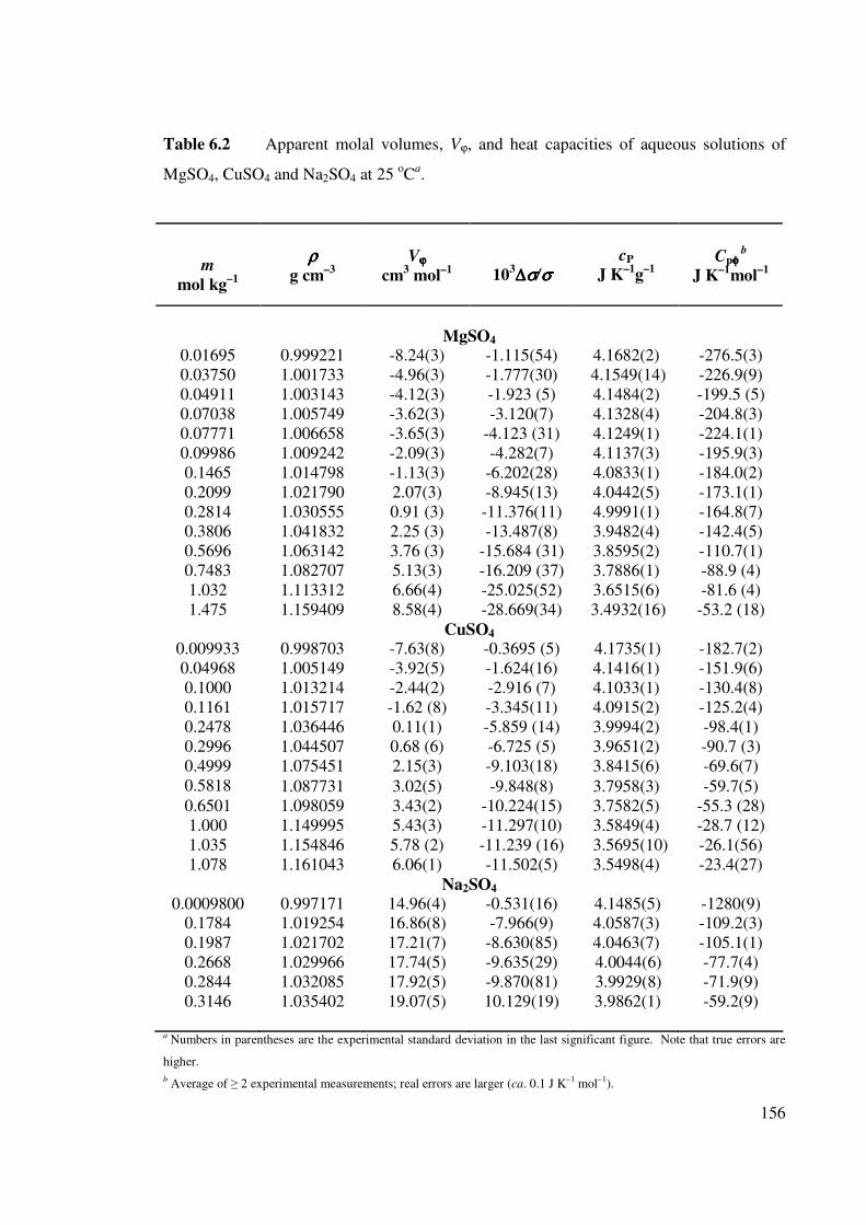
156
Table 6.2 Apparent molal volumes, Vϕ, and heat capacities of aqueous solutions of
MgSO4, CuSO4 and Na2SO4 at 25 oC
a.
m
mol kg–1
ρρρρ
g cm–3
Vϕϕϕϕ
cm3 mol
–1
103∆∆∆∆σσσσ/σσσσ
cP
J K–1
g–1
Cpφφφφ
b
J K–1
mol–1
MgSO4
0.01695 0.999221 -8.24(3) -1.115(54) 4.1682(2) -276.5(3)
0.03750 1.001733 -4.96(3) -1.777(30) 4.1549(14) -226.9(9)
0.04911 1.003143 -4.12(3) -1.923 (5) 4.1484(2) -199.5 (5)
0.07038 1.005749 -3.62(3) -3.120(7) 4.1328(4) -204.8(3)
0.07771 1.006658 -3.65(3) -4.123 (31) 4.1249(1) -224.1(1)
0.09986 1.009242 -2.09(3) -4.282(7) 4.1137(3) -195.9(3)
0.1465 1.014798 -1.13(3) -6.202(28) 4.0833(1) -184.0(2)
0.2099 1.021790 2.07(3) -8.945(13) 4.0442(5) -173.1(1)
0.2814 1.030555 0.91 (3) -11.376(11) 4.9991(1) -164.8(7)
0.3806 1.041832 2.25 (3) -13.487(8) 3.9482(4) -142.4(5)
0.5696 1.063142 3.76 (3) -15.684 (31) 3.8595(2) -110.7(1)
0.7483 1.082707 5.13(3) -16.209 (37) 3.7886(1) -88.9 (4)
1.032 1.113312 6.66(4) -25.025(52) 3.6515(6) -81.6 (4)
1.475 1.159409 8.58(4) -28.669(34) 3.4932(16) -53.2 (18)
CuSO4 0.009933 0.998703 -7.63(8) -0.3695 (5) 4.1735(1) -182.7(2)
0.04968 1.005149 -3.92(5) -1.624(16) 4.1416(1) -151.9(6)
0.1000 1.013214 -2.44(2) -2.916 (7) 4.1033(1) -130.4(8)
0.1161 1.015717 -1.62 (8) -3.345(11) 4.0915(2) -125.2(4)
0.2478 1.036446 0.11(1) -5.859 (14) 3.9994(2) -98.4(1)
0.2996 1.044507 0.68 (6) -6.725 (5) 3.9651(2) -90.7 (3)
1.075451 2.15(3) -9.103(18) 3.8415(6) -69.6(7) 0.4999
0.5818 1.087731 3.02(5) -9.848(8) 3.7958(3) -59.7(5)
0.6501 1.098059 3.43(2) -10.224(15) 3.7582(5) -55.3 (28)
1.000 1.149995 5.43(3) -11.297(10) 3.5849(4) -28.7 (12)
1.035 1.154846 5.78 (2) -11.239 (16) 3.5695(10) -26.1(56)
1.078 1.161043 6.06(1) -11.502(5) 3.5498(4) -23.4(27)
Na2SO4
0.0009800
0.1784
0.1987
0.2668
0.2844
0.3146
0.997171
1.019254
1.021702
1.029966
1.032085
1.035402
14.96(4)
16.86(8)
17.21(7)
17.74(5)
17.92(5)
19.07(5)
-0.531(16)
-7.966(9)
-8.630(85)
-9.635(29)
-9.870(81)
10.129(19)
4.1485(5)
4.0587(3)
4.0463(7)
4.0044(6)
3.9929(8)
3.9862(1)
-1280(9)
-109.2(3)
-105.1(1)
-77.7(4)
-71.9(9)
-59.2(9)
a Numbers in parentheses are the experimental standard deviation in the last significant figure. Note that true errors are
higher.
b Average of ≥ 2 experimental measurements; real errors are larger (ca. 0.1 J K
–1 mol
–1).
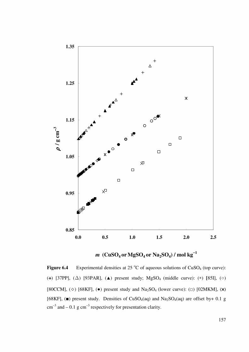
157
0.85
0.95
1.05
1.15
1.25
1.35
0.0 0.5 1.0 1.5 2.0 2.5
m (CuSO4 or MgSO4 or Na2SO4) / mol kg−−−−1
ρρ ρρ /
g c
m−− −−
3
Figure 6.4 Experimental densities at 25
oC of aqueous solutions of CuSO4 (top curve):
(++++) [37PP], (∆) [93PAR], () present study; MgSO4 (middle curve): (∗) [85I], ()
[80CCM], () [68KF], () present study and Na2SO4 (lower curve): () [02MKM], (××××)
[68KF], () present study. Densities of CuSO4(aq) and Na2SO4(aq) are offset by+ 0.1 g
cm–3
and – 0.1 g cm–3
respectively for presentation clarity.
158
The data on the CuSO4(aq) and MgSO4(aq) solutions show the negative values of the Vϕ in
dilute solutions. The same phenomenon has been observed by Pearce and Pumplin [37PP]
for CuSO4 and MgSO4 solutions. The negative and low values for CuSO4 are an indication
of the large electrostriction of the solvent produced by the cupric ions, the water dipoles
being compressed around the cupric ion by the high charge-density of the ion.
The present Vϕ values for CuSO4(aq) (Figure 6.6) are lower than those of Puchalska et al.
[93PAR] but higher than those of Pearce and Pumplin [37PP]. However all Vϕ data show a
similar trend and the present Vϕ (CuSO4(aq)) agree well with recent unpublished data from
the present laboratory [04ET]. The present Vϕ values for MgSO4(aq) agree well with
literature values [68KF, 80CCM, 85I] at higher concentrations but deviate significantly at
lower concentrations. The apparent molal volumes of Na2SO4 solutions agree well with
calculated literature results [02MKM] except the value obtained for the lowest
concentration (1×10⁻³
mol kg–1
) due to the uncertainty in ∆ρ. Thus it was ignored.
Densities of ternary aqueous solutions of Na2SO4-CuSO4, Na2SO4-MgSO4 and CuSO4-
MgSO4 were measured at constant ionic strength at 25 oC. The results are presented in
Figure 6.8 and show that the mixtures of Na2SO4-MgSO4 and CuSO4-MgSO4 show ideal
(Young’s rule) mixing while the mixtures of Na2SO4-CuSO4 deviate from linearity.
The apparent molal volumes of the ternary mixture, CuSO4-Na2SO4-H2O at constant ionic
strength (I = 1.00) are summarized in Table 6.3. The results are presented in Figure 6.10
as a function of ionic strength fraction y3,
2233
333
mImI
mIy
+= (6.24)
where m2 and m3 are the molalities of electrolytes (2) Na2SO4 and (3) CuSO4 and I is the
stoichiometric ionic strength, 2
2
1ii
z∑ν . (I = 4 and 3 for 2-2 and 2-1 electrolytes
respectively).
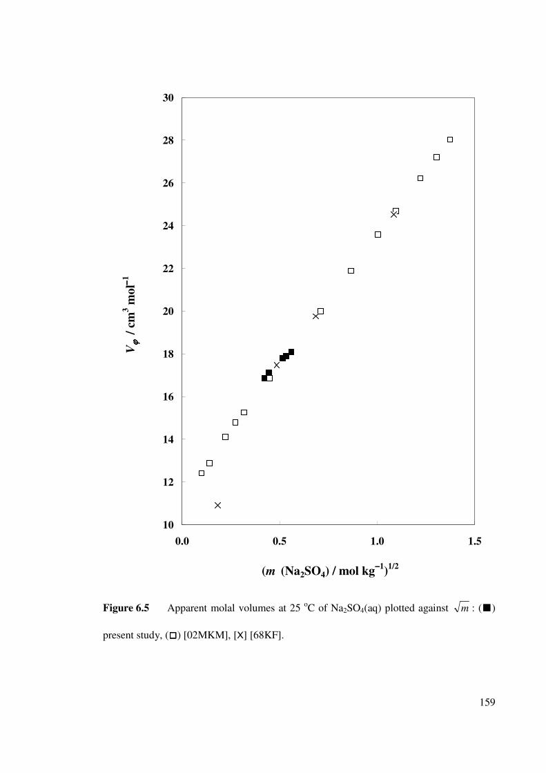
159
10
12
14
16
18
20
22
24
26
28
30
0.0 0.5 1.0 1.5
(m (Na2SO4) / mol kg−−−−1
)1/2
Vϕϕ ϕϕ
/ c
m3 m
ol−− −−
1
Figure 6.5 Apparent molal volumes at 25 oC of Na2SO4(aq) plotted against m : ()
present study, () [02MKM], [X] [68KF].
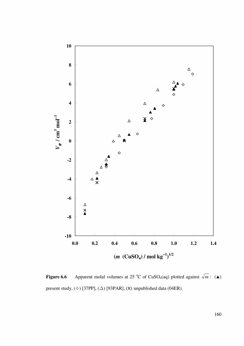
160
-10
-8
-6
-4
-2
0
2
4
6
8
10
0.0 0.2 0.4 0.6 0.8 1.0 1.2 1.4
(m (CuSO4) / mol kg−−−−1
)1/2
Vϕϕ ϕϕ
/ c
m3 m
ol−− −−
1
Figure 6.6 Apparent molal volumes at 25 oC of CuSO4(aq) plotted against m : ()
present study, () [37PP], (∆) [93PAR], (X) unpublished data (04ER).
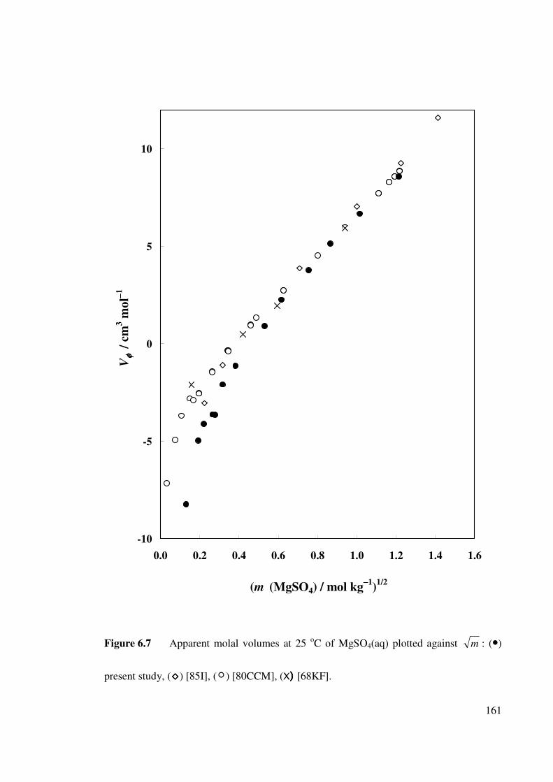
161
-10
-5
0
5
10
0.0 0.2 0.4 0.6 0.8 1.0 1.2 1.4 1.6
(m (MgSO4) / mol kg−−−−1
)1/2
Vφφ φφ
/ c
m3 m
ol−− −−
1
Figure 6.7 Apparent molal volumes at 25 oC of MgSO4(aq) plotted against m : (•)
present study, () [85I], () [80CCM], (X) ) ) ) [68KF].
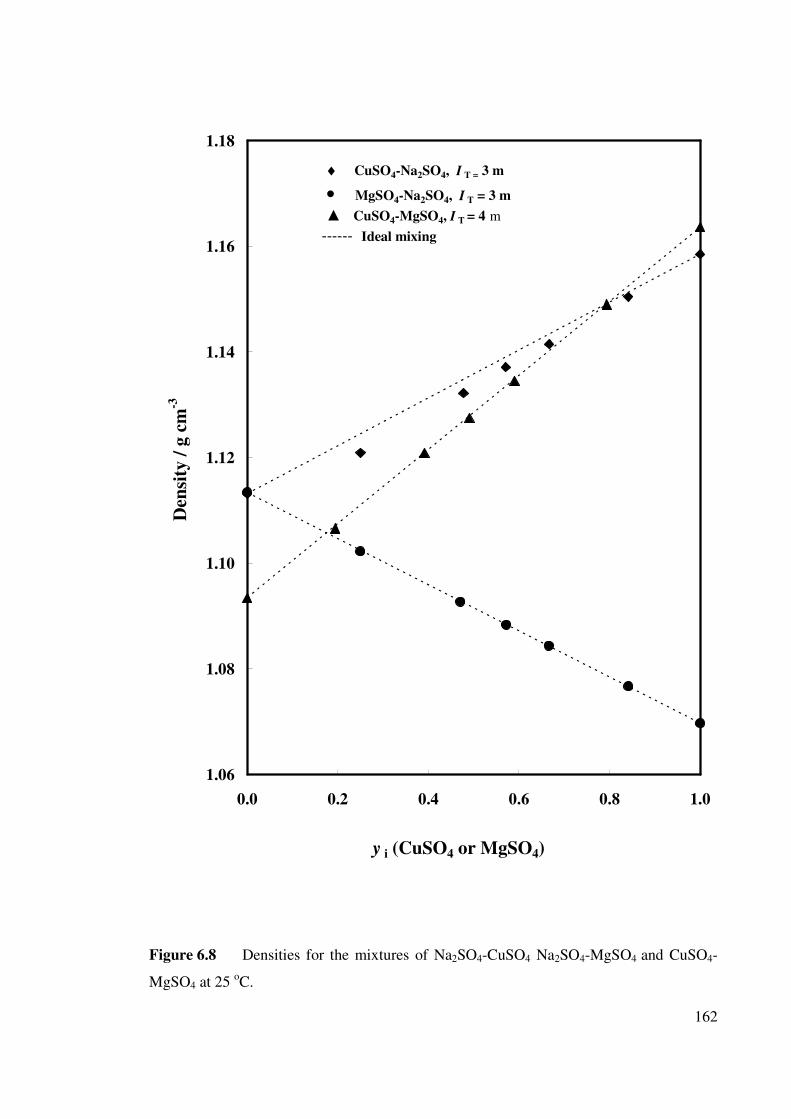
162
1.06
1.08
1.10
1.12
1.14
1.16
1.18
0.0 0.2 0.4 0.6 0.8 1.0
y i (CuSO4 or MgSO4)
Den
sity
/ g
cm
-3
♦ CuSO4-Na2SO4, I T = 3 m
• MgSO4-Na2SO4, I T = 3 m
CuSO4-MgSO4, I T = 4 m
------ Ideal mixing
Figure 6.8 Densities for the mixtures of Na2SO4-CuSO4 Na2SO4-MgSO4 and CuSO4-
MgSO4 at 25 oC.
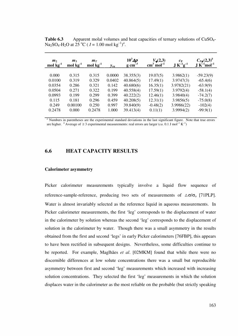
163
Table 6.3 Apparent molal volumes and heat capacities of ternary solutions of CuSO4-
Na2SO4-H2O at 25 oC ( I = 1.00 mol kg
–1)a.
m2
mol kg-1
m3
mol kg-1
mT
mol kg-1
ycu
103∆∆∆∆ρρρρ
g cm–3
Vϕϕϕϕ(2,3)
cm3 mol
–1
cP
J K–1
g–1
CPφφφφ (2,3)b
J K–1
mol–1
0.000 0.315 0.315 0.0000 38.355(3) 19.07(5) 3.9862(1) -59.23(9)
0.0100 0.319 0.329 0.0402 40.864(5) 17.49(1) 3.9747(3) -65.4(6)
0.0354 0.286 0.321 0.142 40.680(6) 16.35(1) 3.9782(21) -63.9(9)
0.0504 0.271 0.322 0.199 40.558(4) 17.59(1) 3.9792(4) -58.1(4)
0.0993 0.199 0.299 0.399 40.222(2) 12.46(1) 3.9840(4) -74.2(7)
0.115 0.181 0.296 0.459 40.208(5) 12.31(1) 3.9856(5) -75.0(8)
0.249 0.00100 0.250 0.997 39.840(9) -0.48(2) 3.9986(22) -102(4)
0.2478 0.000 0.2478 1.000 39.413(4) 0.11(1) 3.9994(2) -99.9(1)
a Numbers in parentheses are the experimental standard deviations in the last significant figure. Note that true errors
are higher. b Average of ≥ 3 experimental measurements: real errors are larger (ca. 0.1 J mol–1 K–1)
6.6 HEAT CAPACITY RESULTS
Calorimeter asymmetry
Picker calorimeter measurements typically involve a liquid flow sequence of
reference-sample-reference, producing two sets of measurements of σ/σo
[71PLP].
Water is almost invariably selected as the reference liquid in aqueous measurements. In
Picker calorimeter measurements, the first ‘leg’ corresponds to the displacement of water
in the calorimeter by solution whereas the second ‘leg’ corresponds to the displacement of
solution in the calorimeter by water. Though there was a small asymmetry in the results
obtained from the first and second ‘legs’ in early Picker calorimeters [76FBP], this appears
to have been rectified in subsequent designs. Nevertheless, some difficulties continue to
be reported. For example, Maglhães et al. [02MKM] found that while there were no
discernible differences at low solute concentrations there was a small but reproducible
asymmetry between first and second ‘leg’ measurements which increased with increasing
solution concentrations. They selected the first ‘leg’ measurements in which the solution
displaces water in the calorimeter as the most reliable on the probable (but strictly speaking
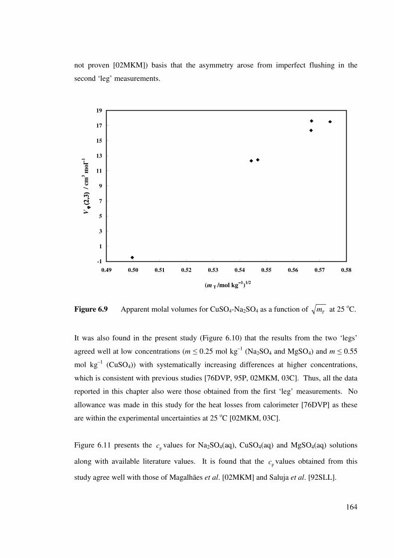
164
not proven [02MKM]) basis that the asymmetry arose from imperfect flushing in the
second ‘leg’ measurements.
-1
1
3
5
7
9
11
13
15
17
19
0.49 0.50 0.51 0.52 0.53 0.54 0.55 0.56 0.57 0.58
(m T /mol kg−−−−1
)1/2
Vϕ
ϕ
ϕ
ϕ
(2
,3)
(2,3
) (2
,3)
(2,3
) / c
m3 m
ol−− −−
1
Figure 6.9 Apparent molal volumes for CuSO4-Na2SO4 as a function of T
m at 25 oC.
It was also found in the present study (Figure 6.10) that the results from the two ‘legs’
agreed well at low concentrations (m ≤ 0.25 mol kg–1
(Na2SO4 and MgSO4) and m ≤ 0.55
mol kg–1
(CuSO4)) with systematically increasing differences at higher concentrations,
which is consistent with previous studies [76DVP, 95P, 02MKM, 03C]. Thus, all the data
reported in this chapter also were those obtained from the first ‘leg’ measurements. No
allowance was made in this study for the heat losses from calorimeter [76DVP] as these
are within the experimental uncertainties at 25 oC [02MKM, 03C].
Figure 6.11 presents the pc values for Na2SO4(aq), CuSO4(aq) and MgSO4(aq) solutions
along with available literature values. It is found that the pc values obtained from this
study agree well with those of Magalhães et al. [02MKM] and Saluja et al. [92SLL].
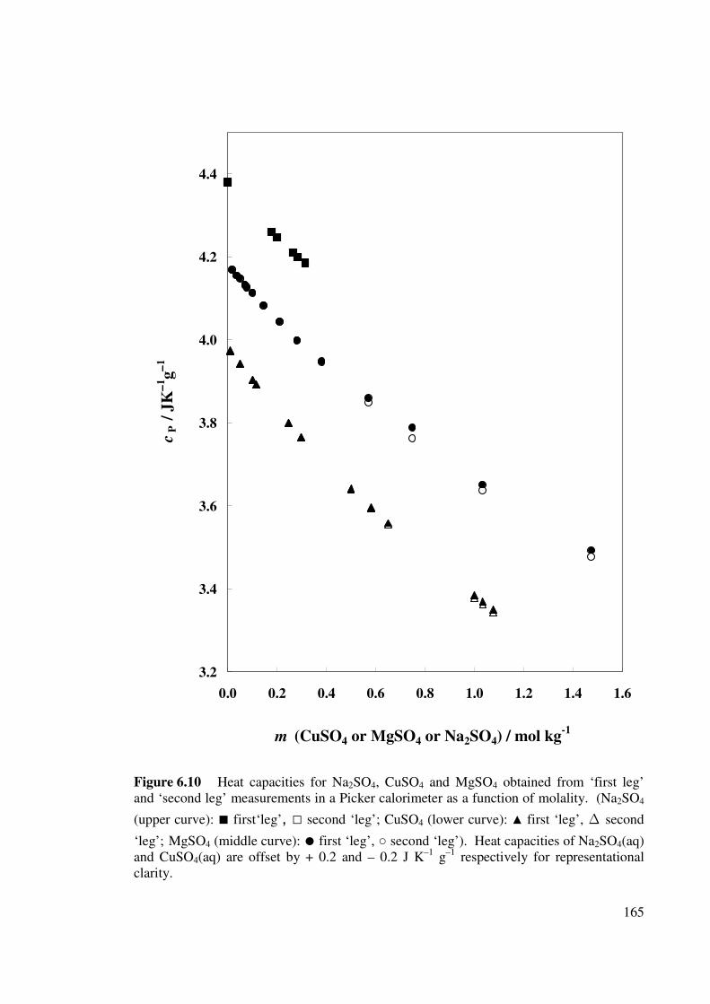
165
3.2
3.4
3.6
3.8
4.0
4.2
4.4
0.0 0.2 0.4 0.6 0.8 1.0 1.2 1.4 1.6
m (CuSO4 or MgSO4 or Na2SO4) / mol kg-1
cP
/
JK
−− −−1g
−− −−1
Figure 6.10 Heat capacities for Na2SO4, CuSO4 and MgSO4 obtained from ‘first leg’
and ‘second leg’ measurements in a Picker calorimeter as a function of molality. (Na2SO4
(upper curve): first‘leg’, second ‘leg’; CuSO4 (lower curve): first ‘leg’, ∆ second
‘leg’; MgSO4 (middle curve): first ‘leg’, second ‘leg’). Heat capacities of Na2SO4(aq)
and CuSO4(aq) are offset by + 0.2 and – 0.2 J K–1
g–1
respectively for representational
clarity.
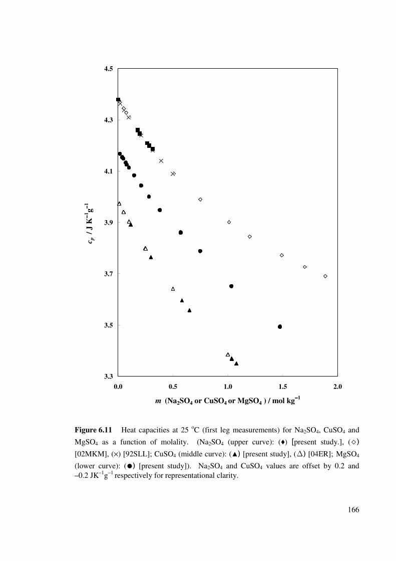
166
3.3
3.5
3.7
3.9
4.1
4.3
4.5
0.0 0.5 1.0 1.5 2.0
m (Na2SO4 or CuSO4 or MgSO4 ) / mol kg−−−−1
cp
/ J
K−− −−
1g
−− −−1
Figure 6.11 Heat capacities at 25 oC (first leg measurements) for Na2SO4, CuSO4 and
MgSO4 as a function of molality. (Na2SO4 (upper curve): (♦) [present study.], ()
[02MKM], (×) [92SLL]; CuSO4 (middle curve): () [present study], (∆) [04ER]; MgSO4
(lower curve): ( ) [present study]). Na2SO4 and CuSO4 values are offset by 0.2 and
–0.2 JK–1
g−1
respectively for representational clarity.
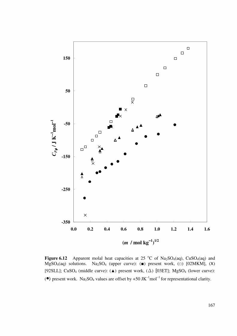
167
-350
-250
-150
-50
50
150
0.0 0.2 0.4 0.6 0.8 1.0 1.2 1.4 1.6
(m / mol kg−−−−1
)1/2
CP
φφ φφ /
J K
−− −−1m
ol−− −−
1
Figure 6.12 Apparent molal heat capacities at 25 oC of Na2SO4(aq), CuSO4(aq) and
MgSO4(aq) solutions. Na2SO4 (upper curve): () present work, () [02MKM], (X)
[92SLL]; CuSO4 (middle curve): () present work, (∆) [03ET]; MgSO4 (lower curve):
(•) present work. Na2SO4 values are offset by +50 JK–1
mol−1
for representational clarity.
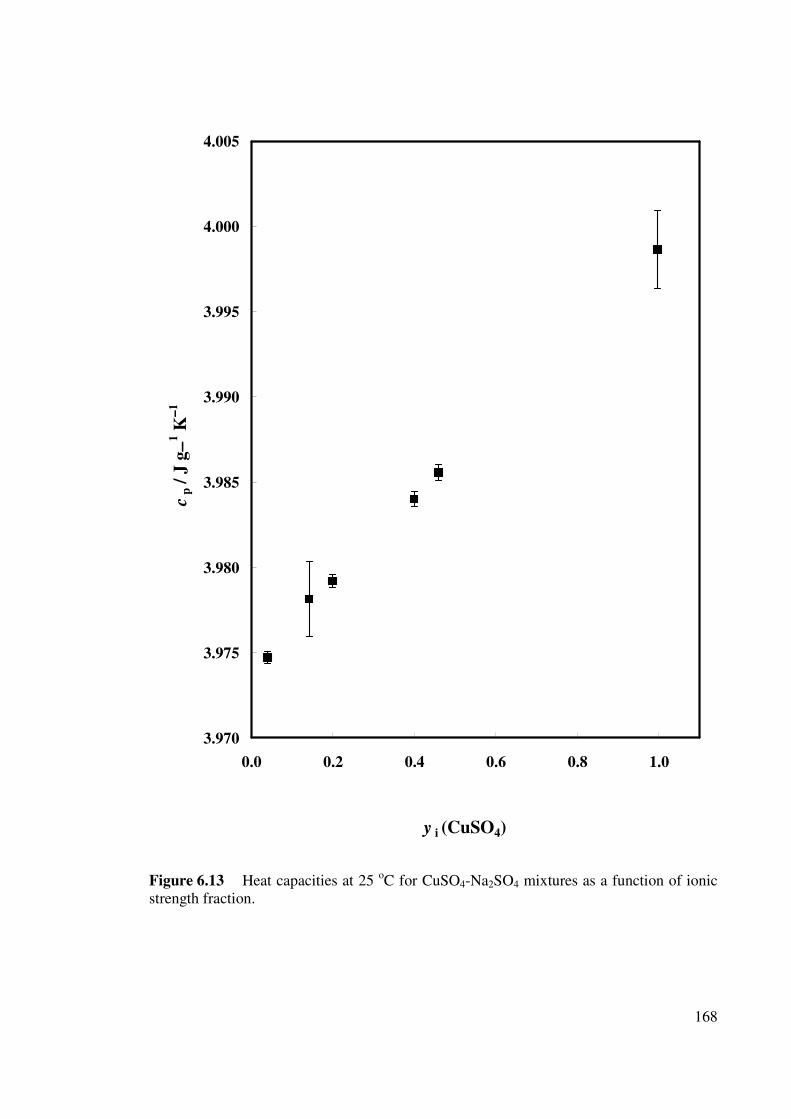
168
3.970
3.975
3.980
3.985
3.990
3.995
4.000
4.005
0.0 0.2 0.4 0.6 0.8 1.0
y i (CuSO4)
cp /
J g
−− −−1 K
−− −−1
Figure 6.13 Heat capacities at 25 oC for CuSO4-Na2SO4 mixtures as a function of ionic
strength fraction.
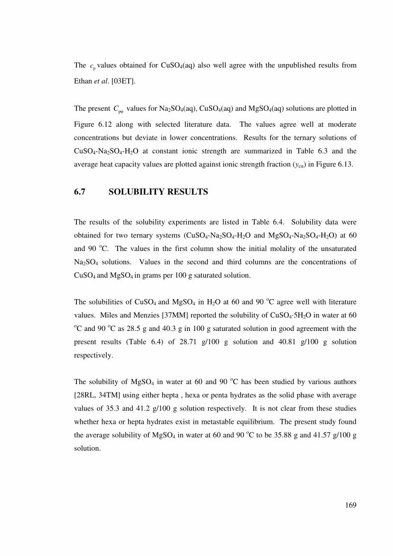
169
The pc values obtained for CuSO4(aq) also well agree with the unpublished results from
Ethan et al. [03ET].
The present pφC values for Na2SO4(aq), CuSO4(aq) and MgSO4(aq) solutions are plotted in
Figure 6.12 along with selected literature data. The values agree well at moderate
concentrations but deviate in lower concentrations. Results for the ternary solutions of
CuSO4-Na2SO4-H2O at constant ionic strength are summarized in Table 6.3 and the
average heat capacity values are plotted against ionic strength fraction (ycu) in Figure 6.13.
6.7 SOLUBILITY RESULTS
The results of the solubility experiments are listed in Table 6.4. Solubility data were
obtained for two ternary systems (CuSO4-Na2SO4-H2O and MgSO4-Na2SO4-H2O) at 60
and 90 oC. The values in the first column show the initial molality of the unsaturated
Na2SO4 solutions. Values in the second and third columns are the concentrations of
CuSO4 and MgSO4 in grams per 100 g saturated solution.
The solubilities of CuSO4 and MgSO4 in H2O at 60 and 90 oC agree well with literature
values. Miles and Menzies [37MM] reported the solubility of CuSO4·5H2O in water at 60
oC and 90
oC as 28.5 g and 40.3 g in 100 g saturated solution in good agreement with the
present results (Table 6.4) of 28.71 g/100 g solution and 40.81 g/100 g solution
respectively.
The solubility of MgSO4 in water at 60 and 90 oC has been studied by various authors
[28RL, 34TM] using either hepta , hexa or penta hydrates as the solid phase with average
values of 35.3 and 41.2 g/100 g solution respectively. It is not clear from these studies
whether hexa or hepta hydrates exist in metastable equilibrium. The present study found
the average solubility of MgSO4 in water at 60 and 90 oC to be 35.88 g and 41.57 g/100 g
solution.
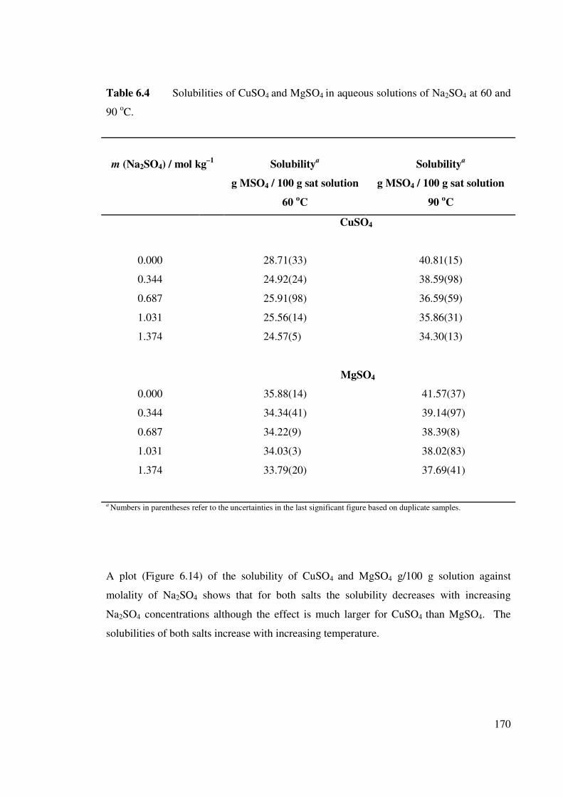
170
Table 6.4 Solubilities of CuSO4 and MgSO4 in aqueous solutions of Na2SO4 at 60 and
90 oC.
m (Na2SO4) / mol kg–1
Solubilitya
g MSO4 / 100 g sat solution
60 oC
Solubilitya
g MSO4 / 100 g sat solution
90 oC
CuSO4
0.000 28.71(33) 40.81(15)
0.344 24.92(24) 38.59(98)
0.687 25.91(98) 36.59(59)
1.031 25.56(14) 35.86(31)
1.374 24.57(5) 34.30(13)
MgSO4
0.000 35.88(14) 41.57(37)
0.344 34.34(41) 39.14(97)
0.687 34.22(9) 38.39(8)
1.031 34.03(3) 38.02(83)
1.374
33.79(20) 37.69(41)
a Numbers in parentheses refer to the uncertainties in the last significant figure based on duplicate samples.
A plot (Figure 6.14) of the solubility of CuSO4 and MgSO4 g/100 g solution against
molality of Na2SO4 shows that for both salts the solubility decreases with increasing
Na2SO4 concentrations although the effect is much larger for CuSO4 than MgSO4. The
solubilities of both salts increase with increasing temperature.
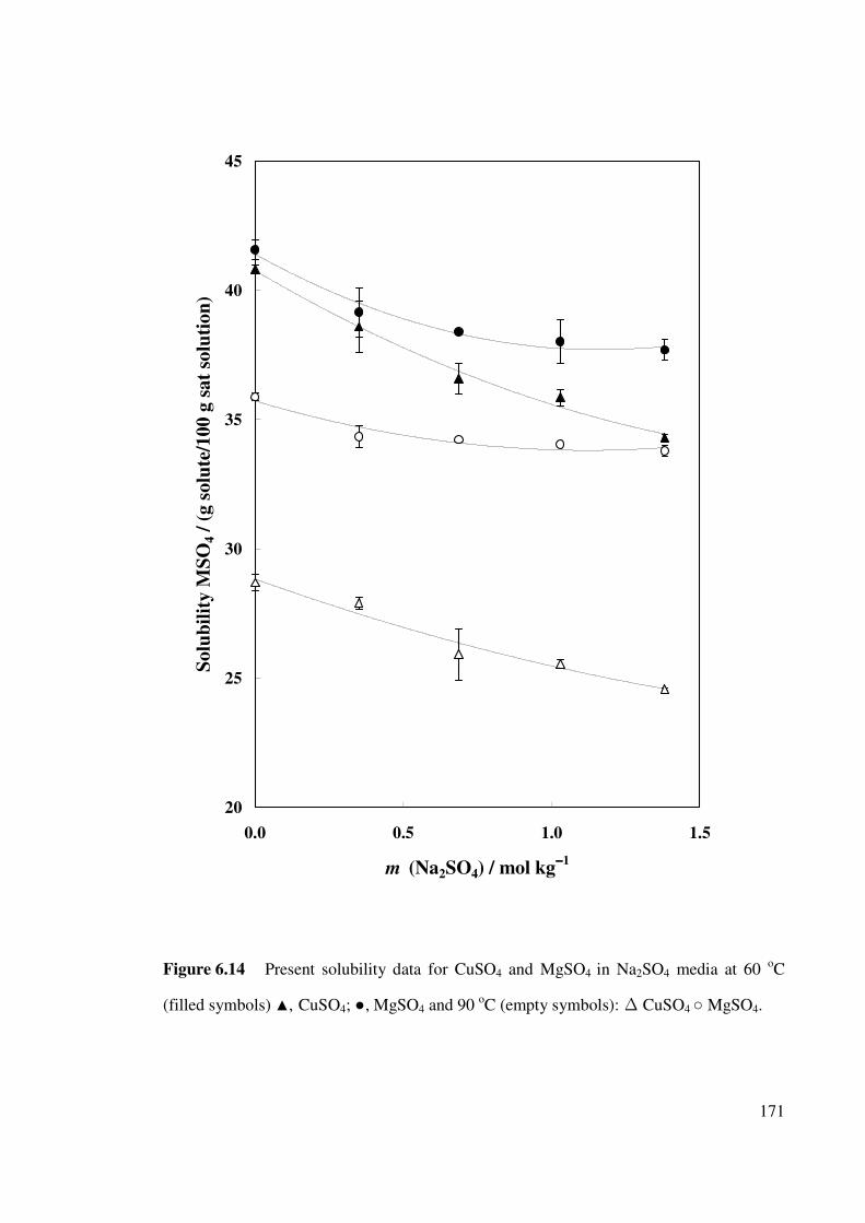
171
20
25
30
35
40
45
0.0 0.5 1.0 1.5
m (Na2SO4) / mol kg−−−−1
So
lub
ilit
y M
SO
4 /
(g
so
lute
/10
0 g
sa
t so
luti
on
)
Figure 6.14 Present solubility data for CuSO4 and MgSO4 in Na2SO4 media at 60 oC
(filled symbols) , CuSO4; , MgSO4 and 90 oC (empty symbols): ∆ CuSO4 MgSO4.
172
6.8 VISCOSITY RESULTS
The observed densities and dynamic viscosities of ternary mixtures of CuSO4-Na2SO4-
H2O, MgSO4-Na2SO4-H2O and CuSO4-MgSO4-H2O at 25 oC are presented in Table 6.5.
The results are also plotted in Figure 6.15, as a function of ionic strength fraction yi.
Dotted lines refer to the values calculated using Equation 6.18. As expected, the
viscosities (Figure 6.15) of all three systems do not behave linearly. It is apparent that the
viscosities of all of the mixtures show clear negative departure from ‘Young’s rule’
behaviour with the CuSO4-Na2SO4-H2O system showing the largest deviations.
The data presented in Figure 6.15 contain aqueous mixtures (CuSO4-Na2SO4, MgSO4-
Na2SO4) of 1:2 ternary systems of constant ionic strength of 3 obviously contain Na2SO4
as a common constituent. 2:2 ternary mixture of aqueous solution of (CuSO4-MgSO4) 2:2
ternary system has been studied at ionic strength of 4.
However, all the systems studied, including those at different ionic strengths and different
charge types, showed negative deviations and these were always close to symmetrical
[03HMS]. Negative deviations have been reported by various authors [03HMS] for
various ternary systems. Even though there is no obvious reason for this behaviour, it has
been shown by Hefter et al. [03HMS] that the size of the deviations from ideal (Young’s
rule) behaviour are related to the differences in the viscosities of the (binary) end-member
solutions.
The viscosities of the binary (end-member) solutions agree reasonably with the literature
values. Pigoniowa’s [73Pi] viscosity values 1.469 (0.752 mol L–1
) and 1.702 mPa s (1.005
mol L–1
) for aqueous CuSO4 solution at temperatures 25 oC reasonably agree with the
present study values 1.4673 mPa s (0.7500 mol L–1
) and 1.7576 mPa s (1.000 mol L–1
).
Korosi and Fabuss’s [68KF] values for the viscosities of aqueous Na2SO4 solution at 25oC
1.3432 mPa s (1.0 mol L–1
) are in fairly good agreement with the present study
value1.3676 mPa s (1.000 mol L–1
).
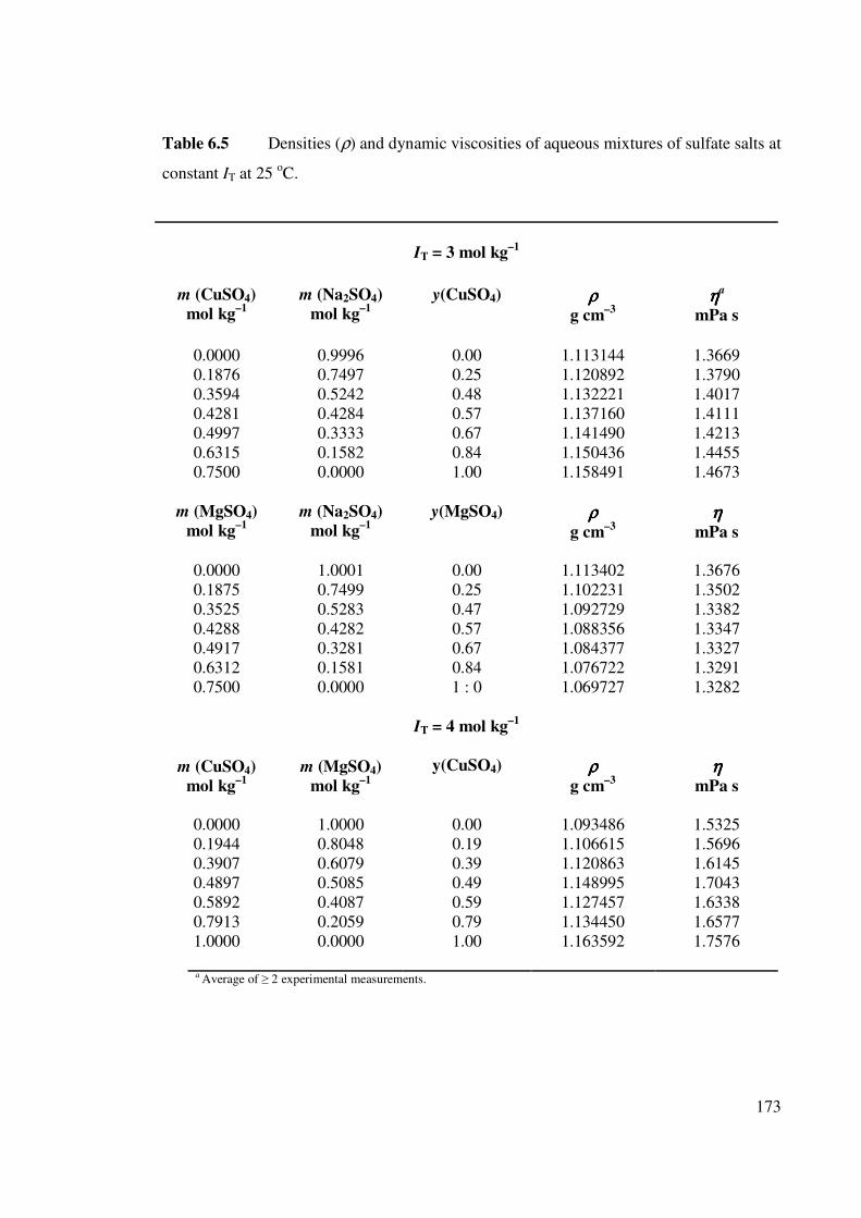
173
Table 6.5 Densities (ρ) and dynamic viscosities of aqueous mixtures of sulfate salts at
constant IT at 25 oC.
IT = 3 mol kg–1
m (CuSO4)
mol kg–1
m (Na2SO4)
mol kg–1
y(CuSO4)
ρρρρ
g cm–3
ηηηηa
mPa s
0.0000 0.9996 0.00 1.113144 1.3669
0.1876 0.7497 0.25 1.120892 1.3790
0.3594 0.5242 0.48 1.132221 1.4017
0.4281 0.4284 0.57 1.137160 1.4111
0.4997 0.3333 0.67 1.141490 1.4213
0.6315 0.1582 0.84 1.150436 1.4455
0.7500 0.0000 1.00 1.158491 1.4673
m (MgSO4)
mol kg–1
m (Na2SO4)
mol kg–1
y(MgSO4) ρρρρ
g cm–3
ηηηη
mPa s
0.0000 1.0001 0.00 1.113402 1.3676
0.1875 0.7499 0.25 1.102231 1.3502
0.3525 0.5283 0.47 1.092729 1.3382
0.4288 0.4282 0.57 1.088356 1.3347
0.4917 0.3281 0.67 1.084377 1.3327
0.6312 0.1581 0.84 1.076722 1.3291
0.7500 0.0000 1 : 0 1.069727 1.3282
IT = 4 mol kg–1
m (CuSO4)
mol kg–1
m (MgSO4)
mol kg–1
y(CuSO4) ρρρρ
g cm–3
ηηηη
mPa s
0.0000 1.0000 0.00 1.093486 1.5325
0.1944 0.8048 0.19 1.106615 1.5696
0.3907 0.6079 0.39 1.120863 1.6145
0.4897 0.5085 0.49 1.148995 1.7043
0.5892 0.4087 0.59 1.127457 1.6338
0.7913 0.2059 0.79 1.134450 1.6577
1.0000 0.0000 1.00 1.163592 1.7576
a Average of ≥ 2 experimental measurements.
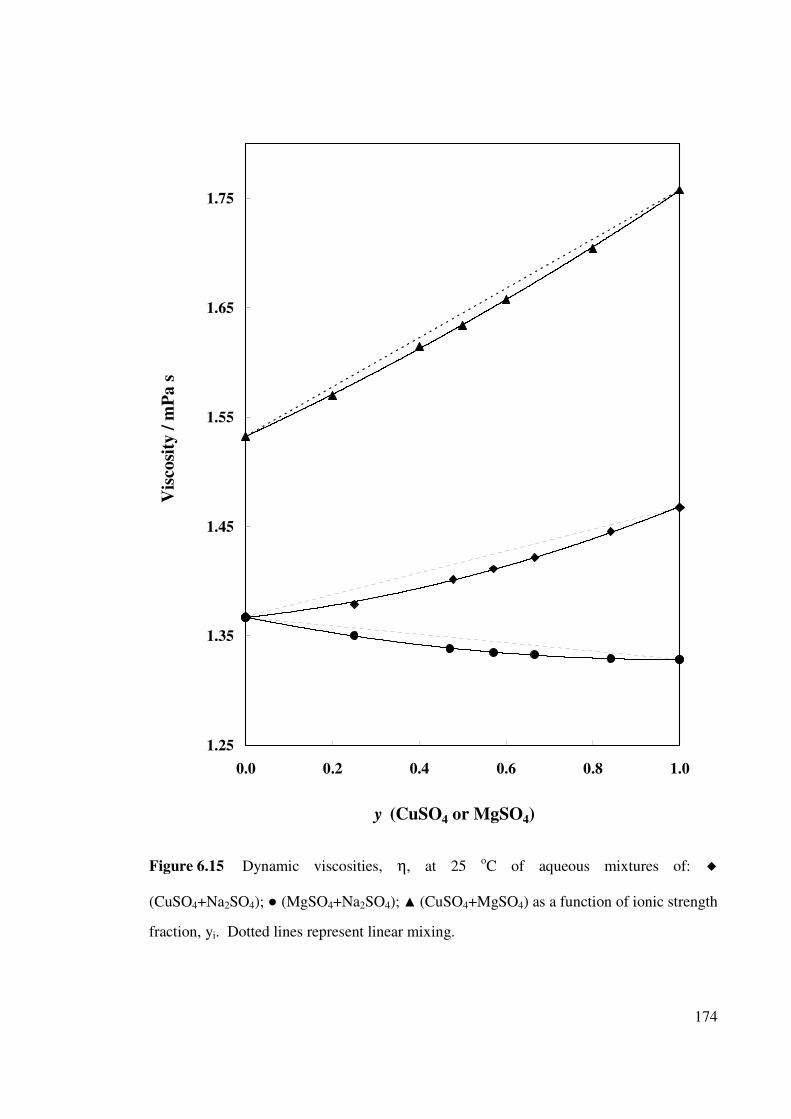
174
1.25
1.35
1.45
1.55
1.65
1.75
0.0 0.2 0.4 0.6 0.8 1.0
y (CuSO4 or MgSO4)
Vis
co
sity
/ m
Pa
s
Figure 6.15 Dynamic viscosities, η, at 25 oC of aqueous mixtures of:
(CuSO4+Na2SO4); (MgSO4+Na2SO4); (CuSO4+MgSO4) as a function of ionic strength
fraction, yi. Dotted lines represent linear mixing.
175
6.9 CONCLUDING REMARKS
Physicochemical properties such as osmotic coefficients, densities, heat capacities,
solubilities and also viscosities of CuSO4, Na2SO4 and MgSO4 and their ternary mixtures
have been measured and the results fitted to the relevant models. It was found that 2:2
electrolyte mixtures of CuSO4 and MgSO4 follow the Zdanovskii’s rule but 1:2 mixtures
electrolytes did not. Densities of 2:2 electrolyte mixtures also followed Young’s rule more
closely than 1:2/2:2 mixtures with Na2SO4-CuSO4 showing larger deviations than
Na2SO4-MgSO4. These results cannot be explained in any simple way by differences in
ion association.
The present study also shows that the viscosities of the CuSO4-MgSO4-H2O system follow
a linear mixing rule. On the other hand the behaviour of the Na2SO4-CuSO4-H2O system
is rather different from that of the CuSO4-MgSO4-H2O and the MgSO4-Na2SO4-H2O
systems.
176
Chapter Seven
Conclusions and future work
This thesis has described a quantitative investigation of the interaction between Cu2+
(aq)
and SO42–
(aq) ions in aqueous solution. UV-Visible spectrophotometry was used to
determine the formation constant of 0
4CuSO (aq) in solutions of ionic strength ranging from
0.05 to 4.0 M in NaClO4 media. High precision copper(II) ion-selective electrode
potentiometry was also used to determine formation constant constants in solutions of
ionic strength ranging from 0.05 to 5.0 M in NaClO4 media. It has been established that
the values of the formation constants for 0
4CuSO (aq) obtained from UV-Visible
spectrophotometric studies were always lower than those obtained by Cu2+
-ISE
potentiometry. No convincing evidence was found for any higher order complexes (or
‘triple ions’).
Further studies were carried out using dielectric relaxation spectroscopy to provide the
information about the nature of the various ion-pairs present in the aqueous solutions of
copper(II) sulfate. Consistent with the well-established Eigen-Tamn mechanism, the
dielectric spectra indicated the presence of three ion-pair types (doubly solvent-separated,
solvent-shared and contact ion pairs) at appropriate solute concentrations and temperatures.
The stepwise formation constants for these ion pair types gave a value of the overall
association in good agreement with o
AK value obtained from the potentiometric
measurements at 25 oC. The existence of significant concentrations of solvent-separated
ion-pairs is consistent with the UV-Visible spectrophotometry results being lower than
those obtained from potentiometry.
A detailed calorimetric titration study of the interaction between Cu2+
(aq) and −2
4SO (aq)
has provided, for the first time, reliable values for enthalpy and entropy changes for the
formation of 0
4CuSO (aq) as a function of ionic strength over the range 0.1 ≤ I/M (NaClO4)
177
≤ 4.79. The standard state values of ∆Ho
and ∆S
o for the overall association were obtained
by interpolation of the data to infinite dilution and good agreement with literature data was
achieved.
This thesis is also concerned with the ternary solutions of CuSO4 mixed with either MgSO4
of Na2SO4. Systematic measurements of osmotic coefficients, densities, heat capacities
and viscosities at 25 oC and solubilities at 60 and 90
oC were made in mixed electrolyte
solutions of 1:2 and 2:2 electrolyte solutions. Since the overall ion association constants
for 0
4CuSO (aq) and 0
4MgSO (aq) are similar, their mixtures could expect to behave in
similar manner. All the data obtained from the present work suggest that mixtures of
CuSO4 with Na2SO4 show greater deviation from ‘ideal’ mixing than does MgSO4.
Future work
A number of obvious extensions to this study present themselves. First, it would be
interesting to extend UV-Visible spectrophotometry and Cu(II)-ISE potentiometry studies
of the formation constant for 0
4CuSO (aq) to higher temperatures. The Cu(II)-ISE is
applicable to the temperature range 0 - 80 o
C and with appropriate cell designs to minimize
solvent evaporation such measurements would be useful to confirm the less precise DRS
determination of o
AK at higher temperatures and to check the persistence of the difference
from the UV-Vis values.
The DRS information obtained in Chapter 4 could possibly be more closely related to the
UV-Visible (Chapter 2) and potentiometry (Chapter 3) values if the DRS measurements
involve the measurements of CuSO4 in solutions at constant ionic strength made up with
NaClO4 for example. Note, however, that it would be difficult to study the mixtures of
CuSO4 since such solutions would undoubtedly exhibit very high conductivities.
With regard to the enthalpy and entropy of formation studies, dilution experiments could
be extended to dilution of each solution in water and dilution of Cu(ClO4)2 and Na2SO4
into their mixtures to study the possible reason for higher dilution values.
178
Isopiestic studies can be extended to several constant water activities to obtain the
behaviour of osmotic coefficients with different water activities. Further studies of
densities, heat capacities and viscosities of ternary mixtures of copper sulfate solutions at
various constant ionic strengths could be important to predict the behaviour of such
mixtures of practical importance such as those relevant to the industry.
180
References
[16HP] H. D. Holler and E. L. Peffer, J. Amer. Chem. Soc., 1916, 38, 1021.
[19F] H. W. Foote, J. Ind. Eng. Chem., 1919, 11, 629.
[22B] J. N. Bronsted, J. Amer. Chem. Soc. 1922, 44, 877.
[23DH] P. Debye and E. Huckel, Physik. Z., 1923, 24, 185.
[24AG] E. H. Archibald and W. A. Gale, J. Amer. Chem. Soc., 1924, 46, 1760.
[26AB] G. Agde and H. Barkholt, Angew. Chem., 1926, 39, 851.
[26B] N. Bjerrum, Kgl. Danske Videnskab. Selskab, 1926, 7, 1.
[27K] A. Kupper, Caliche, 1927, 8, 467.
[27R] H. L. Robson, J. Amer. Chem. Soc., 1927, 49, 2772.
[28RL] A. Smits, J. Rinse and K. L. H. Louwe, Z. Physik, 1928, 135, 78.
[29S] W. Schroder, Angew. Chem., 1929, 42, 1076.
[33JT] G. Jones and S. K. Talley, J. Amer.Chem. Soc., 1933, 55, 4124.
[34TM] H. H. Ting and W. L. McCabe, J. Ind. Eng. Chem., 1934, 26, 1207.
[35G] E. A. Guggenheim, Phil. Mag., 1935, 19, 58.
[36S] G. Scatchard, Chem. Rev., 1936, 19, 309.
181
[37MM] F. T. Miles and A. W. C. Menzies, J. Amer. Chem. Soc., 1937, 59, 2395.
[37PP] J. N. Pearce and G. G. Pumplin, J. Amer. Chem. Soc., 1937, 59, 1221.
[38OG] B. B. Owen and R. G. Gurry, J. Amer. Chem. Soc., 1938, 60, 3074.
[38Z] A. B Zdanovskii, J. Phys. Chem (USSR)., 1936, 6, 70.
[41S] A. Seidell (ed), Solubilities of Inorganic and Organic Compounds, Vol.
2, 3rd edn., Van Nostrand, New York , 1941.
[48F] S. Fronaeus, Komplexsystem Hos Kopper, Gleerupska Univ.,
Bokhandeln, Lund, 1948, 139.
[49Na] R. Nasanen, Acta Chem. Scand., 1949, 3, 179.
[49Nb] R. Nasanen, Acta Chem. Scand., 1949, 3, 959.
[50F] S. Fronaeus, Acta Chem. Scand., 1950, 4, 72.
[51NL] R. Nasanen and P. Lumme, Acta Chem. Scand., 1951, 5, 13.
[51W] P. A. H. Wyatt, Trans. Faraday Soc., 1951, 47, 656.
[51Y] T. F. Young, Rec. Chem. Prog., 1951, 12, 81.
[52BP] D. Berg and A. Patterson Jr., J. Amer. Chem. Soc., 1952, 74, 4704.
[52JM] H. W. Jones and C. B. Monk, J. Amer. Chem. Soc., 1952, 74, 4.
[53N] R. Nasanen, Suomen Kem., 1953, 26B, 67.
[54YS] T. F. Young and M. B. Smith, J. Phys. Chem., 1954, 58, 716.
182
[55BP] P. G. M. Brown and J. E. Prue, Proc. Roy. Soc., 1955, A232, 320.
[56BDM] W. D. Bale, E. W. Davies and C. B. Monk, Trans. Faraday Soc., 1956,
52, 816.
[56K] J. Kenttamaa, Suomen Kem., 1956, 29B, 59.
[57C] S. R. Cohen, J. Phys. Chem., 1957, 61, 1670.
[57DOP] W. G. Davies, R. J. Otter and J. E. Prue, Disc. Faraday Soc., 1957, 24.
[57K] M. Kaminsky, Z. Phys. Chem., 1957, 12, 206.
[57N] G. H. Nancollas, Disc. Faraday Soc., 1957, 24, 108.
[58HO] H. S. Harned and B. B. Owen, The Physical Chemistry of Electrolytic
Solutions, 3rd edn, Reinhold, New York, 1958.
[58N] V. S. K. Nair and G. H. Nancollas, J. Chem. Soc., 1958, 706.
[59NN] V. S. K. Nair and G. H. Nancollas, J. Chem. Soc., 1959, 3934.
[59RR] F. J. C. Rossotti and H. Rossotti, J. Phys. Chem., 1959, 63, 1041.
[59SA] S. Suryanarayan and S. Alamelu, Bull. Chem. Soc. Jpn., 1959, 32, 333.
[61PF] A. Patterson, Jr. and H. Freitag, J. Electrochem. Soc.,1961, 108, 529.
[61RR] F. J. C. Rossotti and H. Rossotti, The Determination of Stability
Constants, McGraw-Hill, New York, 1961.
[62AY] G. Atkinson and M. Yokoi., J. Phys. Chem., 1962, 84, 1520.
[62D] C. W. Davies, Ion Association, Butterworths., London, 1962.
183
[62ETa] M. Eigen and K. Tamm, Z. Elektrochem., 1962, 66, 93.
[62ETb] M. Eigen and K. Tamm, Z. Elektrochem., 1962, 66, 107.
[63HIC] J. D. Hale, R. M. Izatt, and J. J. Christensen, J. Phys. Chem., 1963, 67,
2605.
[63LZ] L. Lamberts and F. Zeeger-Huyskens, J. Chim. Phys., 1963, 20, 435.
[64HP] R. E. Hester and R. A. Plane, Inorg. Chem., 1964, 3, 769.
[65CIH] J. J. Christensen, R. M. Izatt and L. D. Hansen, Rev. Sci. Instr., 1965,
36, 779.
[65G] S. R. Gunn, J. Phys. Chem., 1965, 69, 2902.
[65M] R. A. Matheson, J. Phys. Chem., 1965, 69, 1537.
[65P] R. Pottel, Ber. Bunsen Ges. Phys. Chem., 1965, 5, 363.
[65SM] R. G. Seys and C. B. Monk, J. Chem. Soc., 1965, 2452.
[65TSO] N. Tanaka, Y. Saito and H. Ogino, Bull. Chem. Soc. Jpn., 1965, 38, 984.
[65YK] M. Yokoi and E. Kubota, J. Chem. Soc. Jpn., 1965, 86, 894.
[66A] Anonymous, Unicam SP800 Operating Instructions, Unicam
instruments, 1966.
[66CIH] J. J Christensen, R. M. Izatt, L. D. Hansen and J. A. Partridge, J. Phys.
Chem., 1966, 70, 2003.
[66FKH] B. M. Fabuss, A. Korosi and A. K. M. S. Huq, J. Chem. Eng. Data,
1966, 11, 325.
184
[66N] G. H. Nancollas, Interactions in Electrolyte Solutions, Elsevier, New
York, 1966.
[66PVA] P. Paoletti, A. Vacca and D. Arenare, J. Phys. Chem., 1966, 70, 194.
[67AP] L. Abello and G. Pannetier, Bull. Soc. Chim. Fr., 1967, 3752.
[68CG] S. Cabani and P. Gianni, J. Chem. Soc. (A), 1968, 547.
[68HP] P. Hemmes and S. Petrucci, J. Phys. Chem., 1968, 72, 3986.
[68IES] R. M. Izatt, D. Eatough, R. L. Snow and J. J. Christensen, J. Phys.
Chem., 1968, 72, 1208.
[68KF] A. Korosi and B. M. Fabuss, J. Chem. Eng. Data, 1968, 13, 548.
[68M] R. A. Matheson, J. Phys. Chem., 1968, 72, 3330.
[68Ma] G. Maass, Z. Phys. Chem., N. F. 1968, 60, 138.
[68MMM] V. E. Mironov, Y. A. Makashev, I. Y. Mavrina and D. M. Markhaeva,
Russ. J. Phys. Chem., 1968, 42, 2987.
[68PK] K. G. Plass and A. Kehl, Acustica, 1968, 20, 360.
[68W] Y. C. Wu, J. Phys. Chem., 1968, 72, 2663.
[68WRS] Y. C. Wu, R. M. Rush and G. Scatchard, J. Phys. Chem., 1968, 72,
4048.
[68YMK] M. Yokoi, Y. Mori, E. Kubota and K. Murata, Nippon Kagaku Zasshi,
1968, 89, 1192.
[69BG] F. Becker and R. Grundmann, Z. Phys. Chem. NF, 1969, 66, 137.
185
[69FHP] F. Fittipaldi, P. Hemmes and S. Petrucci, Acustica, 1969, 21, 228.
[69GG] A. W. Gardner and E. Glueckauf, Proc. Roy. Soc. Lond. A. 1969, 313,
131.
[69IEC] R. M. Izatt, D. Eatough, J. J. Christensen and C. H. Bartholomew, J.
Chem. Soc. A, 1969, 45.
[69IECa] R. M. Izatt, D. Eatough, J. J. Christensen and C. H. Bartholomew, J.
Chem. Soc. A, 1969, 47.
[69SF] G. Schwarzenbach and H. Flaschka, Complexometric Titrations, 2nd
edn., Methuen, London, 1969.
[69SM] D. Singh and A. Mishra, Ind. J. Chem., 1969, 7, 1219.
[70B] M. T. Beck, Chemistry of Complex Equilibria, Van Nostrand Reinhold,
London, 1970.
[70BBT] A. Bechteler, K. G. Breitschwerdt and K. Tamm, J. Chem. Phys., 1970,
52, 2975.
[70FHP] F. Fittipaldi, P. Hemmes and S. Petrucci, Acustica, 1970, 23, 322.
[70FMH] K. Fritsh, C. J. Montrose, J. L. Hunter and J. F. Dill, J. Phys. Chem.,
1970, 52, 2242.
[70HP] P. Hemmes and S. Petrucci, J. Phys. Chem., 1970, 74, 467.
[70L] J. W. Larson, J. Phys. Chem., 1970, 74, 3392.
[70MMM] V. E. Mironov, Y. A. Makashev, I. Y. Mavrina and M. M.
Kryzhanovskii, Russ. J. Inorg. Chem, 1970, 15, 668.
186
[70RC] A. M. Rowe and J. C. S. Chou, J. Chem. Eng. Data, 1970, 15, 61.
[70RS] R. A. Robinson and R. H. Stokes, Electrolyte Solutions, 2nd edn.,
Butterworths, London, 1970.
[70SW] L. G. Sillen and B. Warnqvist, Arki. Kemi., 1970, 31, 377.
[71HPP] E. M Hanna, A. D. Pethybridge and J. E. Prue, Electrochim. Acta, 1971,
16, 677.
[71KVP] M. M. Kryzhanovskii, Y. A. Volokhov, L. N.Pavlov, N. I. Eremin and
V. E. Mironov, Z. Prikl. Khim., 1971, 44, 476 (E: 484).
[71M] W. J. Mader and L. T. Grady, in Physical Methods of Chemistry. Part V,
Determination of Thermodynamic and Surface Properties, 1971.
[71Mi] F. Millero, Chem. Rev., 1971, 71, 147.
[71MKA] Y. A. Makashev, F. Y. Kul'ba, M. I. Agaf, Y. A. Volokhov and V. E.
Mironov, Russ .J. Phys. Chem., 1971, 45, 414.
[71PLP] P. Picker, P. A. Leduc, P. R. Philip and J. E. Desnoyers, J. Chem.
Thermodyn., 1971, 3, 631.
[72A] S. Ahrland, Coord. Chem. Rev., 1972, 8, 21.
[72DP] J. E. Desnoyers and G. Perron, J. Solution Chem., 1972, 1, 199.
[72ECI] D. Eatough, J. J. Christensen and R. M. Izatt, Thermochim. Acta, 1972,
3, 219.
[72GP] G. Gritzner and R. F. Philips, J. Chem. Eng. Data, 1972, 17, 425.
[72H] G. T. Hefter, J. Electroanal. Chem., 1972, 39, 345.
187
[72P] K. S. Pitzer, J. Chem. Soc. Faraday Trans. II, 1972, 68, 101.
[73B] C. F. J. Böttcher, Theory of Electric Polarisation, 2nd edn, Elsevier,
Amsterdam, 1973.
[73CGE] J. J. Christensen, J. W. Gardner, D. J. Eatough and R. M. Izatt, Rev. Sci.
Instrum., 1973, 44, 481.
[73HP] G. R. Hedwig and H. K. J. Powell, J. Chem. Soc., Dalton Trans., 1973,
798.
[73K] S. Katayama, Bull. Chem. Soc. Jpn., 1973, 46, 106.
[73P] H. K. J. Powell, J. Chem. Soc., Dalton Trans., 1973, 1947.
[73Pi] J. D. Pigoniowa, Pol. J. Chem., 1973, 47, 2183.
[74BRM] V. V. Blokhin, L. I. Razmyslova, Y. A. Makashev, and V. E. Mironov,
Russ. J. Phys. Chem, 1974, 48, 82.
[75ECI] D. J. Eatough, J. J. Christensen, and R. M. Izatt, J. Chem.Thermodyn.,
1975, 7, 417.
[75K] J. Koryta, Ion Selective Electrodes, Cambridge University Press,
Cambridge, 1975.
[75T] R. Tamamushi, Bull. Chem. Soc. Jpn., 1975, 48, 705.
[75YY] H. Yokoyama and H. Yamatera, Bull. Chem. Soc. Jpn, 1975, 48, 2719.
[76BM] C. F. Baes Jr and R. E. Mesmer, The Hydrolysis of Cations, Wiley
Interscience, New York, 1976.
188
[76DVP] J. E. Desnoyers, C. de Visser, G. Perron and P. Picker, J. Solution
Chem., 1976, 5, 605.
[76FB] J. Fortier and G. C. Benson, J. Solution Chem., 1976, 5, 605.
[76FBP] J. L. Fortier, G. C. Benson and P.Picker, J. Chem. Thermodyn., 1976, 8,
289.
[76T] R. F Tylecote, History of Metallurgy, The Metals Society, London,
1976.
[76W] J. D. Winefordner, Trace Analysis, Spectroscopic Methods for Elements,
Vol 46, Wiley Interscience, New York, 1976.
[77AH] K. G. Ashurst and R. D. Hancock, Natl. Inst. Metall. report, Randburg,
South Africa, 1977, 1914, 1.
[77AHa] K. G. Ashurst and R. D. Hancock, J. Chem. Soc. Dalton Trans., 1977,
1701.
[77H] P. Hedvig, Dielectric Properties of Polymers, Hilger, Bristol, 1977.
[77K] S. Katayama, Rikagaku Kenkyusho Hokoku, 1977, 53, 212 (Chem.
Abstr., 1978, 89, 49644q).
[77KFT] T. N. Koneva, V. A. Fedorov and G. L. Trofimov, Russ. J. Phys. Chem.,
1977, 51, 470.
[77STK] K. Shimizu, N. Tsuchihashi and Y. Kondo, Rev. Phys. Chem. Jpn, 1977,
47, 80.
[77WH] E. M. Woolley and L. G. Hepler, Can. J. Chem., 1977, 55, 158.
189
[78BB] C. F. Böttcher and P. Bordewijk, Theory of Electric Polarization, 2nd
edn., Elsevier, Amsterdam, 1978, Vol 2.
[78CP] E. A. S. Cavell and S. Petrucci, J. Chem. Soc. Faraday Trans, 1978, 74,
1019.
[78FF] F. H. Fisher and A. P. Fox, J. Solution Chem., 1978, 7, 561.
[78R] H. S. Rossotti, The Study of Ionic Equilibria, Longmans, London, 1978.
[79C] K. Cammann, Working with Ion Selective Electrodes, Springer-verlag,
Berlin, 1979.
[79GCE] J. F. Gal, C. Calleri, L. Elegant and M. Azzaro, Bull. Chim. Soc. Fr.,
1979, 311.
[79HH] L. G. Hepler and H. P. Hopkins, Rev. Inorg. Chem., 1979, 1, 333.
[79LMZ] K. Laqua, W. H. Melhuish and M. Zander, Pure Appl. Chem., 1979, 51,
1.
[79M] F. J. Millero, in Activity Coefficients in Electrolyte Solutions, R. M.
Pytkowicz, (Ed.), CRC Press, BocaRaton, U.S.A., 1979, Vol 2, Ch. 2.
[79N] J. O. Nriagu (Ed.), Copper in the Environment, Wiley-Interscience, New
York, U.S.A., 1979.
[79P] R. M. Pytkowicz, in Activity Coefficients in Electrolyte Solutions, R. M.
Pytkowicz (Ed.), CRC Press, BocaRaton, U.S.A., 1979, Vol 1, Ch. 1.
[79PR] R. F. Platford, in Activity Coefficients in Electrolyte Solutions, K. S.
Pitzer (Ed), 2nd edn., CRC Press, Boca Raton, U.S.A., 1979, Vol 1,
p.65.
190
[80CCM] C. A Chen, J. H. Chen and F. J. Millero, J. Chem. Eng. Data, 1980, 25,
307.
[80I] T. Isono, Rikagaku Kenkyusho Hokoku, 1980, 56, 103.
[80PLD] D. C. Price, H. Larsson and W. G. Davenport, Nouv. J. Chim. 1980, 4, 7.
[81FK] K. Fujita and M. Kimura, J. Raman Spectrosc., 1981, 11, 108.
[81KKC] J. Kestin, H. E. Khalifa and R. J. Correia, J. Phys. Chem. Ref. Data,
1981, 10, 71.
[81RM] J. A. Rard and D. G. Miller, J. Chem. Eng. Data, 1981, 26, 33.
[81WR] R. Wachter and K. Riederer, Pure Appl. Chem., 1981, 53, 1301.
[81YY] H. Yokoyama and H. Yamatera, Bull. Chem. Soc. Jpn., 1981, 54, 2286.
[82DKA] A. Dadgar, D. Khorsandi and G. Atkinson, J. Phys. Chem., 1982, 86,
3829.
[82H] W. J. Hayes, Pesticides Studied in Man, William and Wilkins,
Baltimore, U.S.A., 1982.
[82Ha] D. C. Harris, Quantitative Chemical Analysis, W. H Freeman, San
Francisco, U.S.A. 1982.
[82He] G. T. Hefter, Anal. Chem., 1982, 54, 2518.
[83B] L. M. Blinov, Electro-Optical and Magneto-Optical Properties of
Liquid Crystals, Wiley, Chichester, U.K.,1983.
[83HK] D. Hartley and H. Kidd (ed.), The Agrochemicals Handbook, Royal
Society of Chemistry, Nottingham, U.K., 1983.
191
[83J] J. C. Justice, Comprehensive Treatise of Electrochemistry, Vol 5, Ch 2,
B.E. Conway, J.O. Bockris and E. Yeager (Ed); 1983.
[83Jo] A. K. Jonscher, Dielectric Relaxation in Solids, Chelsea Dielectric
Press, London, 1983.
[83KS] J. S. Koryta, Ion Selective Electrodes, 2nd edn, Cambridge University
Press, Cambridge, 1983
[83W] C. R. Worthing (Ed.), The Pesticide Manual, British Crop Protection
Council, Croydon, U.K., 1983.
[83Wa] (a) I. Wadsö, Pure Appl. Chem., 1983, 55, 3. (b) I. Wadsö, Pure Appl.
Chem., 1983, 55, 515. (c) I. Wadsö, Pure Appl. Chem., 1983, 55, 528.
[84H] G. T. Hefter, J. Solution Chem., 1984, 13, 179.
[84NLS] M. G. Nordmark, J. Layne, A. Schon, J. Suurkuusk and I. Wadsö, J.
Biomed. Biophy. Methods, 1984, 10, 187.
[84S] E. P. Serjeant, Potentiometry and Potentiometric Titrations, John Wiley,
New York, 1984.
[85GMM] (a) H. Gampp, M. Maeder, C. J. Meyer and A. D. Zuberbuehler,
Talanta, 1985, 32, 95. (b) H. Gampp, M. Maeder, C. J. Meyer and A.D.
Zuberbuehler, Talanta, 1985, 32, 257. (c) H. Gampp, M. Maeder, C. J.
Meyer and A. D. Zuberbuehler, Talanta, 1985, 32, 1133.
[85I] T. Isono, Pikagaku Kenkyusho, 1985, 60, 53.
[85LY] Q. Liu and M. Yang, Huaxe Xuebao, 1985, 43, 126.
[85M] J. M. Montgomery, Water Treatment Principles and Design, John
Wiley., New York, 1985.
192
[85Mi] F. P. Millero, Pure App. Chem., 1985, 57, 1015.
[85MMW] P. M. May, K. Murray and D. R. Williams, Talanta, 1985, 32, 483.
[85SGZ] N. Schmelzer, M. Grigo, B. Zorn and J. Einfeldt, Wissenschaftliche
Zeitschrift De Wilhelm-Pieck-Universitaet Rostock, Naturwissenscha-
ftliche Reihe, 1985, 34, 25.(ISSN 0863-1204)
[86GMM] H. Gampp, M. Maeder, C. J. Meyer and A. D. Zuberbuehler, Talanta,
1986, 33, 943.
[86PP] R. C. Phutela and K. S. Pitzer, J. Chem. Eng. Data, 1986, 31, 320.
[86ZCR] Z. F. Zemaitis, D. M. Clarke, M. Rafal and N. C. Scrivner, Handbook of
Aqueous Electrolyte Thermodynamics, Design Institute for Physical
Property Data, 1986.
[88HHT] J. K. Hovey, L. G. Hepler and P. R. Tremaine, Thermochim. Acta, 1988,
126, 245.
[88MA] H. Majima and Y. Awakura, Metall. Tran., 1988, 19B, 347.
[88MM] A. E. Martell and R. J. Motekaitis, The Determination and Use of
Stability Constants, VCH publishers, New York, 1988.
[88MMW] P. M. May, K. Murray and D. R. Williams, Talanta, 1988, 35, 825.
[88P] S. Prakash, Advanced Inorganic Chemistry, 16th edn., U.K., 1988,
p.364.
[88WAB] R. C. Weast, M. Astle and W. H. Beyre, CRC Hand Book of Chemistry
& Physics, 68th edn., CRC Press, Boca Rato, U.S.A., 1988.
193
[89ACM] G. Arena, R. Cali, G. Maccarrone and R. Purrello, Thermochim. Acta,
1989, 155, 354.
[89JBM] H. Jeffery, L. Bassett, J. Mendham and R. C. Denney, Vogel’s Textbook
of Quantitative Chemical Analysis, 5th edn., Longman Scientific, New
York, 1989.
[89MBR] S. Mallick, B. Behera and S. Rath, J. Electrochem. Soc. India., 1989, 38,
203.
[89R] J. A. Rard, J. Chem. Thermodyn., 1989, 21, 539.
[90A] P. W. Atkins, Physical Chemistry, 4th edn., Oxford Press, 1990.
[90AW] D. G. Archer and P. J. Wang, J. Phys. Chem. Ref. Data, 1990, 19, 371.
[90B] R. F. Brennan, Autral. J. Exp. Agric., 1990, 30, 687.
[90BBB] J. Barthel, R. Buchner, K. Bachhuber, H. Hetzenauer, M. Kleebauer and
H. Ortmaier, Pure Appl. Chem., 1990, 62, 2287.
[90C] B. W. Clare, unpublished, 1990.
[90F] R. E. Fifoot, Modern Plastic Encyclopedia, McGraw-Hill, New York,
1990, Vol. 67, p. 26.
[90GLY] L. Guo, C. Y. Liang, J. Z. Yang and Q. T. Liu, J. Coord. Chem., 1990,
21, 43.
[90K] J. Koryta, Anal. Chim. Acta, 1990, 233, 1.
[90MB] D. C. Melchior and R. L. Bassett, Chemical Modeling of Aqueous
Systems II, American Chemical Society, Washington D.C, 1990.
194
[90SAL] D. F. Shriver, P. W. Atkins and C. H. Langford, Inorganic Chemistry,
Oxford University Press, Oxford, 1990.
[90W] S. Wasylkiewicz, Fluid Phase Equili., 1990, 57, 277.
[91BB] J. Barthel and R. Buchner, Pure Appl. Chem., 1991, 63, 1473.
[91BBB] J. Barthel, K. Bachhuber, R. Buchner, H. Hetzenauer and M. Kleebauer,
Ber. Bunsen-Ges. Phys. Chem. 1991, 95, 853.
[91BW] L. Briggner and I. Wadsö, J. Biochem. Biophys. Methods, 1991, 22, 101.
[91DU] R. A. Day and A. L. Underwood, Quantitative Analysis, 6th edn.,
Prentice-Hall Inc., U.S.A., 1991.
[91LC] J. W. Lorimer and R. Cohen-Adad (ed), Solubility Data Series, Vol. 47,
Alkali Metal and Ammonium Chlorides in Water and Heavy Water
(Binary Systems), Pergamon Press, New York, 1991.
[91MMH] P. McLay, P. M. May and G. T. Hefter, The Murdoch CHEMEQUIL
Group Procedures Manual, Murdoch University, Perth Western
Australia, 1991.
[91P] K. S. Pitzer (ed), Activity Coefficients in Electrolyte Solutions, 2nd edn.,
CRC Press, Boca Raton, U.S.A., 1991.
[92BHB] J. Barthel, H. Hetzenauer and R. Buchner, Ber. Bunsen-Ges. Phys.
Chem., 1992, 96, 1424.
[92HP] Hewlett-Packard Co., Basics of measuring the dielectric properties of
materials, HP Application Notes 1217-1, HP Literature number 5091-
3300E, 1992.
195
[92SLL] P. P. S. Saluja, R. J. Lemire and J. C. Leblanc, J. Chem. Thermodyn.,
1992, 24, 181.
[92WG] D. K. Wyatt and L. T. Grady in Physical Methods for Chemistry, Vol 6,
Determination of Thermodynamic Properties, 2nd edn, Wiley, New
York, 1992.
[92ZA] I. D. Zaytsev and G. G. Aseyev, Properties of Aqueous Solutions of
Electrolytes, CRC Press, Boca Raton, U.S.A., 1992.
[93OR] H. Ohtaki and T. Radnai, Chem. Rev., 1993, 93, 1157.
[93PAR] D. Puchalska, G. Atkinson and S. Routh, J. Solution Chem., 1993, 22,
625.
[93A] Annonymous, Thermometric 2250 Series Instruction Manual,
Thermometric AB, Sweden, 1993.
[94BB] R. Buchner and J. Barthel, Annu. Rep. Prog. Chem., Sect. C, 1994, 91,
71.
[94BD] A. K. Biswas and W. G. Davenport, Extractive Metallurgy of Copper,
3rd edn., Pergamon/Elsevier, Oxford, U.K. 1994.
[94BHB] R. Buchner, G. T. Hefter and J. Barthel, J. Chem. Soc. Faraday Trans.,
1994, 90, 2475.
[94KR] I. M. Klotz and R. M. Rosenberg, Chemical Thermodynamics, 5th edn.,
Wiley-Interscience, New York, 1994.
[94MO] K. N. Marsh, and, P. A. G. O’Hare, Solution Calorimetry, Experimental
Thermodynamics, 4th edn, Cambridge University Press, Cambridge,
U.K., 1994.
[94NH] M. S. K. Niazi and M. Hussain, J. Chem. Eng. Data, 1994, 39, 48.
196
[94SMH] P. Sipos, P. M. May, G. T. Hefter and I. Kron, J. Chem. Soc. Chem.
Commun., 1994, 2355.
[95BLM] J. Bobacka, T. Linffors, M. McCarrick, A. Ivaskn and A. Lewenstam,
Anal. Chem., 1995, 67, 3819.
[95C] D. Q. M. Craig, Dielectric Analysis of Pharmaceutical Systems, Taylor
and Francis, London, 1995.
[95JM] H. D. B. Jenkins and Y. Marcus, Chem. Rev., 1995, 95, 2695.
[95P] K. S. Pitzer, Thermodynamics, 3rd edn., McGraw-Hill, New York, 1995.
[96HH] L. G. Hepler and J. K. Hovey, Can. J. Chem., 1996, 74, 639.
[96R] G. M. Ritcey, Austral. Inst. Mining Metal., 1996, 6/96, 251.
[96SWH] D. A. Skoog, D. M. West and F. J. Holler, Fundamentals of Analytical
Chemistry, 7th edn., Saunders, Fort Worth, U.S.A., 1996.
[97BB] R. Buchner and J. Barthel, Ber. Bunsenges. Phys. Chem., 1997, 101,
1509.
[97CHM] S. G. Capewell, G. T. Hefter, P. Sipos and P. M. May, J. Solution
Chem., 1997, 26, 957.
[97GP] I. Grenthe and I. Puigdomenech, Modelling in Aquatic Chemistry,
Nuclear Energy Agency, Organisation for Economic Co-operation and
Development, Paris, 1997.
[97HMM] G. T. Hefter, P. M. May, S. L. Marshall, J. Cornish and I. Kron, Rev.
Sci. Instrum, 1997, 68, 2558.
[97M] Y. Marcus, Ion Properties, Dekker, New York, 1997.
197
[97OMH] M. Obšil, V. Majer, G. T. Hefter and V. Hynek, J. Chem. Eng. Data,
1997, 42, 137.
[97R] J. A. Rard, J. Chem. Thermodyn., 1997, 29, 533.
[97Ru] A. V. Rumyantsev, J. Solution Chem., 1997, 26, 97.
[98AR] D. G. Archer, and J. A. Rard, J. Chem. Eng. Data, 1998, 43, 791.
[98BBE] J. Barthel, R. Buchner, P. N. Eberspächer, M. Münsterer, J. Stauber and
B. Wurm, J. Mol. Liq. 1998, 78, 82.
[98BKK] J. Barthel, H. Krienke and W. Kunz, Physical Chemistry of Electrolyte
Solutions, Springer, New York, 1998.
[98BZ] R. A. Binstead and A. D. Zuberbuehler, SPECFIT Version 2.11,
Revision c, Spectrum Software Associates, Chapel Hill, U.S.A., 1998.
[98CHM] S. G. Capewell, G. T. Hefter and P.M. May, J. Solution Chem., 1998,
27, 865.
[99BCH] R. Buchner, S. G. Capewell, G. T. Hefter and P. M. May, J. Phys. Chem.
B, 1999, 103, 1185.
[99BHM] R. Buchner, G. T. Hefter and P. M. May, J. Phys. Chem. A, 1999, 103,
1.
[99C] S. G. Capewell, PhD Thesis, Murdoch University, Western Australia,
1999.
[99CHM] S. G. Capewell, G. T. Hefter and P. M. May, Rev. Sci. Ins., 1999, 70,
1481.
[99HC] Z. Ha and C. K. Chan, Aerosol Sci. Technol., 1999, 31, 154.
198
[99RC] J. A. Rard and S. L. Clegg, J. Chem. Thermodyn., 1999, 31, 399.
[00GWO] I. Grenthe, H. Wanner, and E. Osthols, Guidelines for the Extrapolation
to Zero Ionic Strength, Thermochemical Data Base Report 2, Germany,
2000.
[00KHE] U. Kaatze, T.O. Hushcha and F. Eggers, J. Solution Chem., 2000, 29,
299.
[00OBM] G. Olofsson, D. Berling, N. Markova, and M. Molund, Thermochim.
Acta, 2000, 347, 31.
[00RCP] J. A. Rard, S. L. Clegg and D. A. Palmer, J. Solution Chem., 2000, 29, 1.
[00SHM] P. Sipos, G. T. Hefter and P. M. May, J. Chem. Eng. Data, 2000, 45,
613.
[00TM] N. G. Tsierkezoz and I. E. Molinou, J. Chem. Eng. Data, 2000, 45, 819.
[00UBU] Y. Umezawa, P. Buhlmann, K. Umezawa, K. Tohda and S. Amemiya,
Pure Appl. Chem., 2000, 72, 1851.
[00W] I. Wadsö, Thermochim. Acta, 2000, 347, 73.
[01BB] R. Buchner and J. Barthel, Annu. Rep. Prog. Chem. Sect. C., 2001, 97,
349.
[01P] W. N. Perera, PhD Thesis, Murdoch University, Western Australia,
2001.
[01SSB] P. Sipos, A. Stanley, S. Bevis, G. T. Hefter and P. M. May, J. Chem.
Eng. Data, 2001, 46, 657.
[01WG] I. Wadsö and R. N. Goldberg, Pure Appl. Chem., 2001, 73, 1625.
199
[02BHS] R. Buchner, C. Hölzl, J. Stauber and J. Barthel, Phys. Chem. Chem.
Phys., 2002, 4, 2169.
[02G] S. V. Gupta, Practical Density Measurement and Hydrometry, Institute
of Physics Publishing, Bristol, U.K., 2002.
[02HMW] G. T. Hefter, Y. Marcus and W. E. Waghorne, Chem. Rev., 2002, 102,
2773.
[02KSL] F. Kremer, A. Schonhals and W. Luck, Broadband Dielectric
Spectroscopy, Springer, Verlag, 2002.
[02MKM] M. C. F. Magalhães, E. Königsberger, P. M. May and G. T. Hefter, J.
Chem. Eng. Data, 2002, 47, 590.
[02MKS] K. Maeda, H. Kuramochi, T. Shinkawa and K. Fukui, J. Chem. Eng.
Data, 2002, 47, 1472.
[03BSM] R. Buchner, F. Samani, P. M. May, P. Sturm and G. T. Hefter,
ChemPhysChem, 2003, 4, 373.
[03C] T. Chen, PhD Thesis, Murdoch University, Western Australia, 2003.
[03CBH] T. Chen, R. Buchner, and G. T. Hefter, J. Phys. Chem. A, 2003, 107,
4025.
[03GMD] M. E. L Guendouzi, A. Mounir and A. Dinane, J. Chem. Thermodyn.,
2003, 35, 209.
[03HMS] G. T. Hefter, P. M. May, P. Sipos and A. Stanley, J. Mol. Liq., 2003,
103, 261.
[03RIH] W. W. Rudolph, G. Irmer and G. T. Hefter, Phys. Chem. Chem. Phys.
2003, 5, 5253.
200
[03T] A. J. Tromans, PhD Thesis, Murdoch University, Western Australia,
2003.
[04BCH] R. Buchner, T. Chen and G. Hefter, J. Phys. Chem. B, 2004, 108, 2365.
[04B] R. Buchner, In Novel Approaches to the Structure and Dynamics of
Liquids, V. A. Durov (Eds), NATO Science Series II, Kluwer, The
Netherlands, 2004, p.133.
[04ER] W. Ethan and T. Rowland, Unpublished data, Murdoch University,
2004.
[04K] J. Kroschwitz (ed.), Kirk-Othmer Encyclopedia of Chemical
Technology, 5th edn., Wiley-Interscience, Hoboken, U.S.A., 2004, Vol.
7, p. 767.
[04LC] M. Laliberte and W. E.Cooper, J. Chem. Eng. Data, 2004, 49, 114.
[04M] M. A. Mortin, J. Chem. Eng. Data, 2004, 49, 94.
[04RST] B. M. Rode, C. F. Schwenk and A. Tongraar, J. Mol. Liq., 2004, 110,
105.
[04SBK] S. Schrödle, R. Buchner and W. Kunz, J. Phys. Chem. B, 2004, 108,
6281.
[05BBP] M. Beŝter-Rogaĉ , V. Babic, T. M. Perger, R. Neueder and J. Barthel, J.
Mol. Liq., 2005, 118, 111.
[05CHB] T. Chen, G. T. Hefter and R. Buchner, J. Solution Chem., 2005, 34,
1045.
[05KEM] E. Königsberger, G. Eriksson, P. M. May and G. T. Hefter, Ind. Eng.
Chem. Res., 2005, 44, 5805.
201
[05MBF] L. P. Mendez De Leo, H. L. Bianchi and R.Fernandez-Prini, J. Chem.
Thermodyn., 2005, 37, 499.
[05TKM] A. Tromans, E. Königsberger, P. M. May and G. T. Hefter, J. Chem.
Eng. Data, 2005, 50, 2019.
[05WXZ] L. Wang, H. Xu, J. Zhao, C. Song and F. Wang, J. Chem. Thermodyn.,
2005, 37, 477.
[06A] Anonymous, Ion-Slective Electrodes Manual, Metrohm Ltd.,
Switzerland, 2006.
[06AHR] C. Akilan, G. T. Hefter, N. Rohman and R. Buchner, J. Phys. Chem. B,
2006, 110, 14961.
[06AHRb] C. Akilan, G. T. Hefter, N. Rohman and R. Buchner, ChemPhys Chem.,
2006, 7, 2319.
[06AZA] (a) I. M. Abdulagatov, A. B. Zeinalova and N. D. Azizov, J. Chem.
Thermodyn., 2006, 38, 179. (b) I. M. Abdulagatov, A. B. Zeinalova and
N. D. Azizov, J. Chem. Eng. Data, 2006, 51, 1645.
[06AZN] I. M. Abdulagatov, A. B. Zeinalova and D. Nazim, J. Chem. Eng. Data,
2006, 51, 1645.
[06CMM] J. Chaboy, A. Muňoz-Páez, P. J.Merkling and E. Sánchez Marcos, J.
Chem. Phys. 2006, 124, 64509.
[06D] A. Dinane, J. Chem. Thermodyn., 2006, 39, 96.
[06He] G. T. Hefter, Pure Appl. Chem., 2006, 78, 1571.
[06MH] Y. Marcus and G. T. Hefter, Chem. Rev., 2006, 7, 2319.
202
[06WMH] A. Wahab, S. Mahiuddin, G. T. Hefter and W. Kunz, J. Chem. Eng.
Data, 2006, 51, 1609.
[07Aa] Anonymous, Properties of copper sulfate, Meridian World Sdn.Bhd.,
Meridianworld.com, accessed March 2007.
[07Ab] Anonymous, Uses of copper compounds, Copper Development
Association, Inc., www.copper.org/compounds, accessed June 2007.
[07HSB] H. Hölzl, S. Schrödle, J. Barthel and R. Buchner in preparation.
[07PBB] K. J. Powell, P. L. Brown, R. H. Byrne, T. Gajda, G. T. Hefter, S.
Sjöberg, and H. Wanner, Pure Appl. Chem., 2007, 79, 895.
[08A] Anonymous, Viscometer operating manual, Schott-Gerätr Gbmh,
Postfach, Hoftheim, Germany, 2008.
[08RIH] W. W. Rudolph, G. Irmer and G. T. Hefter, Unpublished observation.