Download (1496Kb) - SOAS Research Online - SOAS, University of

Tanaka, Tetsuji (2012) Risk Assessment of Food Supply: A Computable General Equilibrium Approach.

PhD Thesis, SOAS (School of Oriental and African Studies)

http://eprints.soas.ac.uk/13627

Copyright © and Moral Rights for this thesis are retained by the author and/or other

copyright owners. A copy can be downloaded for personal non‐commercial research or

study, without prior permission or charge. This thesis cannot be reproduced or quoted

extensively from without first obtaining permission in writing from the copyright holder/s.

The content must not be changed in any way or sold commercially in any format or medium

without the formal permission of the copyright holders.

When referring to this thesis, full bibliographic details including the author, title, awarding

institution and date of the thesis must be given e.g. AUTHOR (year of submission) "Full

thesis title", name of the School or Department, PhD Thesis, pagination.

Risk Assessment of Food Supply: A Computable

General Equilibrium Approach

Tetsuji Tanaka

Thesis submitted for the degree of PhD in Finance and Management

Studies

2012

Department of Financial & Management Studies

School of Oriental and African Studies

University of London

ii | P a g e

Declaration for PhD thesis

I have read and understood regulation 17.9 of the Regulations for students of the School of

Oriental and African Studies concerning plagiarism. I undertake that all the material

presented for examination is my own work and has not been written for me, in whole or in

part, by any other person. I also undertake that any quotation or paraphrase from the

published or unpublished work of another person has been duly acknowledged in the work

which I present for examination.

Signed: Date: 16 April, 2012

iii | P a g e

Chapter 3 is based on work from

Tanaka, T. and Hosoe, N., 2011. Does agricultural trade liberalization increase risks

of supply-side uncertainty?: Effects of productivity shocks and export restrictions on

welfare and food supply in Japan, Food Policy, June 2011, v. 36, iss. 3, pp. 368-77.

I am the lead author of this article. I programmed the model, conducted the

simulations and analysed the results for this research.

Chapter 4, 5, and 6 are based on works from

Tanaka, T. and Hosoe, N., 2011. What drove the crop price hikes in the food crisis?

GRIPS Discussion Papers 11-16, and

Tanaka, T. and Qiu, H., 2011. "Food security for the world poor: factors behind the

2008 grain price rises in least developed countries", manuscript, Department of Financial &

Management Studies, SOAS, University of London.

I am the lead author of these working papers. I programmed the model, conducted the

simulations and analysed the results for the researches.

iv | P a g e

Acknowledgements

I would like to express my deep and respectful gratitude to my supervisor, Professor

Laixiang Sun. Over the course of the past three years, he has given me truly valuable and

practical advice not only on this thesis, but also for my career path. In addition, I would like

to thank Professor Noriyuki Goto, Dr Hiroyuki Kawashima, and Professor Masayoshi

Honma for their very valuable comments on my research work. My gratitude also goes to

my friends, fellow researchers and staff at School of Oriental and African Studies for their

generous supports and encouragement during my PhD study.

I would like to give my special thanks to Dr Nobuhiro Hosoe at National Graduate

Institute for Policy Studies and Dr Huanguang Qiu at Chinese Academy of Sciences who

have supported me not only technically, but also spiritually and financially as collaborators.

Without them, I could not have completed my thesis.

My parents Mr Toshihiko and Mrs Fukiko Tanaka and my brother Shugo Tanaka

deserve a great amount of gratitude for their generosity and assistance. My parents firmly

supported my long student life financially and emotionally. When I faced tough times, they

always offered me warm words and crucial encouragement.

Tetsuji Tanaka

v | P a g e

Abstract

The world’s food markets have experienced significant instability in recent years and

this instability has led to increasing concerns over food security at both the regional and

global levels. This thesis employs an advanced computable general equilibrium (CGE)

approach and conducts empirical research to address three important topics in the

literature of food security assessment.

The first element of the research revisits the long-standing trade liberalisation debate

on Japanese rice imports. The Japanese government has been reluctant to liberalise the rice

trade on the grounds that it would threaten its ‘‘national food security’’ in the events of such

shocks as crop failure and trade embargoes, and it would make the Japanese economy more

dependent upon food imports and, thus, more susceptible to these risks. Using a CGE model

with a Monte Carlo simulation, the research quantifies the welfare impacts of productivity

shocks and export quotas by major rice exporters and finds little evidence of Japan suffering

from such shocks.

The second aspect of the research explores the root causes of the soaring grain prices

in 2008 by assessing the impacts of possible factors on world-market prices of wheat, rice

and maize within a global CGE modelling framework. It is found that the primal actual

demand and supply factors explain only about 20 per cent of the increases in terms of

wheat, rice and maize.

The third part of the research assesses the impact of the escalating world-market grain

price in 2008 on the grain prices in the least developed countries (LCDs), using a world

trade CGE model. It finds that while the price rises of wheat and maize are limitedly

explained by the main real-side factors, over half the rice price hike is accounted for by

export restrictions and oil price spike. The emergence of biofuel production, which is

popularly considered to be one of the most critical driving forces, marginally increases the

vi | P a g e

grain prices of LDCs. This is because LDCs have little import and export of maize, and

feedstock of biofuel (sugar cane and oil seed) does not show strong substitutive effects on

the price of wheat, rice and maize.

Through these analyses, the thesis makes a methodological contribution and identifies

policy implications. The methodological contribution is the application of the Monte Carlo

method to CGE analysis, which made it possible to evaluate the probabilistic impacts of

Japan’s rice trade liberalisation. Policy implications are identified for trade liberalisation,

grain stocks, export restrictions, and biofuel policy including energy price and financial

speculation.

vii | P a g e

Contents 1 Introduction ............................................................................................................... 1

1.1 Motivation and objective .................................................................................. 1

1.2 Methodological issues ....................................................................................... 5

1.3 Note on the database ........................................................................................ 6

1.4 Contributions of the research .......................................................................... 7

1.5 Organisation of the thesis ................................................................................ 9

2 Computable general equilibrium model ................................................................ 10

2.1 Introduction ..................................................................................................... 10

2.2 Social accounting matrix (SAM) .................................................................... 15

2.2.1 Simple social accounting matrix ............................................................ 15

2.2.2 Global social accounting matrix with the GTAP database ................... 19

2.3 CGE model ....................................................................................................... 23

2.3.1 A single country CGE model ................................................................... 23

2.3.2 Calibration ............................................................................................... 34

2.3.3 Standard world CGE model .................................................................... 36

Standard world CGE model equations .................................................................. 41

2.3.4 The modification of the standard CGE model for Chapter 3 ............... 45

2.3.5 The modification of the standard CGE model for Chapters 4, 5 and 6 52

2.4 Conclusion ....................................................................................................... 60

Appendix: list of variables and parameters .............................................................. 61

3 Does agricultural trade liberalisation increase risks of supply-side

uncertainty?: Effects of productivity shocks and export restrictions on welfare and

food supply in Japan ...................................................................................................... 69

3.1 Introduction ..................................................................................................... 69

3.1.1 National food security and Japan’s agricultural policy ........................ 71

3.1.2 The rice trade and its barriers ............................................................... 72

3.1.3 Literature review .................................................................................... 74

3.2 Structure of the world trade CGE model ...................................................... 76

3.3 Simulation scenarios ...................................................................................... 80

3.3.1 Scenario factor 1: Abolition of trade barriers ........................................ 81

viii | P a g e

3.3.2 Scenario factor 2: Productivity shocks ................................................... 82

3.3.3 Scenario factor 3: Emergency stocks...................................................... 85

3.3.4 Scenario factor 4: Export quotas ............................................................ 87

3.4 Simulation results........................................................................................... 88

3.4.1 Deterministic impact of trade liberalisation ......................................... 89

3.4.2 Productivity shocks in the rest of the world .......................................... 90

3.4.3 Productivity shocks in Japan ................................................................. 91

3.4.4 Impact of productivity shocks all over the world .................................. 92

3.4.5 Effectiveness of emergency stocks ......................................................... 93

3.4.6 Impact of export quotas .......................................................................... 95

3.5 Concluding remarks ........................................................................................ 98

Appendix: Sensitivity analysis ................................................................................ 100

A3.1 Sensitivity analysis: Armington elasticity .............................................. 100

A3.2 Sensitivity analysis: Price elasticity of food consumption ..................... 102

A3.3 Sensitivity analysis: Value added aggregation ....................................... 105

A3.4 Sensitivity analysis: Volatility of productivity ........................................ 106

A3.5 Monte Carlo draws and productivity shocks ........................................... 107

4 Driving forces of the grain price hikes on the world’s and LDCs’ markets in

2008: background and literature review .................................................................... 112

4.1 Background and motivation ......................................................................... 112

4.2 Literature review .......................................................................................... 116

4.2.1 Potential factors behind the world grain price increases ................... 116

4.2.2 Contributory factors to grain prices in LDCs ...................................... 125

4.3 Implications to our research ........................................................................ 127

4.4 Conclusion ..................................................................................................... 128


2008: model, data and scenarios ................................................................................. 130

5.1 Introduction ................................................................................................... 130

5.2 Model.............................................................................................................. 130

5.2.1 Model Review ......................................................................................... 130

5.2.2 Model Structure ..................................................................................... 131

ix | P a g e

5.3 Data ................................................................................................................ 133

5.3.1 Regional and sector aggregations ........................................................ 133

5.3.2 Splitting Sectors in the GTAP Database ............................................. 134

5.3.3 Elasticity parameters ............................................................................ 137

5.3.4 Price data ............................................................................................... 138

5.4 Scenarios ........................................................................................................ 139

5.5 Conclusion ..................................................................................................... 141


2008: simulation results and policy implications ...................................................... 142

6.1 Introduction ................................................................................................... 142

6.2 Results: the impacts on the world grain markets ...................................... 142

6.3 Results: the impacts on the LDCs’ grain markets ...................................... 149

6.4 Policy Discussions ......................................................................................... 153

6.5 Conclusion ..................................................................................................... 156

Appendix: Sensitivity Analyses ............................................................................... 158

Decomposition analysis of the world grain price hikes ...................................... 158

Decomposition analysis of the price spikes in LDCs .......................................... 161

7 Conclusion ............................................................................................................. 165

7.1 Introduction ................................................................................................... 165

7.2 Methodological contribution ......................................................................... 167

7.3 Policy implications ........................................................................................ 168

7.3.1 Trade liberalisation ............................................................................... 168

7.3.2 Grain reserves ....................................................................................... 169

7.3.3 Export restriction .................................................................................. 171

7.3.4 Biofuel policy and energy price ............................................................ 172

7.3.5 Regulation of speculation...................................................................... 173

7.4 Limitations of research ................................................................................. 174

Bibliography ................................................................................................................. 176

x | P a g e

List of tables and figures

TableNo. Title Page2.1 Example of a social accounting matrix 172.2 Structure of a global SAM with the GTAP database 212.3 Data for constructing a global SAM provided from the GTAP database 222.4 Dimensions of the elements in the GTAP database 223.1 List of regions and sectors in the model 783.2 Scenario design 813.3 Regression results of paddy rice productivity 833.4 Summary statistics of simulation results for Japan 883.5 Welfare impact in scenarios M and Q 98A3.1 Assumed key elasticity and its alternative values used in sensitivity 100A3.2 Summary statistics of simulation results for Japan (with elasticity of substitution: –30 %) 101A3.3 Summary statistics of simulation results for Japan (with elasticity of substitution: +30 %) 102A3.4 Estimates of price elasticity of rice demand 104A3.5 Summary statistics of simulation results for Japan ( =1.0) 105A3.6 Summary statistics of simulation results for Japan (with elasticity of substitution=0.1) 106A3.7 Summary statistics of simulation results for Japan (with elasticity of substitution=1.0) 106A3.8 Summary statistics of simulation results for Japan (with doubled ) 107A3.9 Summary statistics of the randomized productivity 110A3.10 Correlation between the OLS residuals 1114.1 Estimates of price rise factors 1254.2 Impact estimation on grain prices in developing countries by existing literature 1275.1 Country and sector aggregations 1345.2 Splitting maize and biofuels sectors 1365.3 Biofuel data sources 1375.4 Elasticity parameter values in the model 1385.5 Scenario table 1405.6 Crop and its related market shocks in 2007/2008 1406.1 Decomposition analysis of the grain price hikes 1476.2 Decomposition analysis of grain price hikes in LDCs 152A6.1 Decomposition analysis (the Armington elasticity=20 for agricultural sectors) 159A6.2 Decomposition analysis (the Armington elasticity=-50% for agricultural sectors) 159A6.3 Decomposition analysis (elasticity of substitution for value added=0.1) 159A6.4 Decomposition analysis (elasticity of substitution for value added=1.0) 160A6.5 Decomposition analysis (elasticity of substitution for food composite=1.0) 160A6.6 Decomposition analysis (elasticity of substitution between energy goods=+45%) 160A6.7 Decomposition analysis (elasticity of substitution between energy goods=-45%) 161A6.8 Decomposition analysis (the Armington elasticity=20 for agricultural sectors) 162A6.9 Decomposition analysis (the Armington elasticity=-50% for agricultural sectors) 162A6.10 Decomposition analysis (elasticity of substitution for value added=0.1) 162A6.11 Decomposition analysis (elasticity of substitution for value added=1.0) 163A6.12 Decomposition analysis (elasticity of substitution for food composite=1.0) 163A6.13 Decomposition analysis (elasticity of substitution between energy goods=+45%) 163A6.14 Decomposition analysis (elasticity of substitution between energy goods=-45%) 164

fε

rσ

xi | P a g e

FiguresNo. Title Page2.1 Concept of CGE model 112.2 The structure of a single-country model 232.3 The structure of a standard world CGE model 372.4 The structure of household consumption for Chapter 3 512.5 Model structure in Chapters 4,5 and 6 562.6 Model structure of household consumption in Chapters 4, 5 and 6 563.1 Productivity fluctuations of paddy rice 733.2 Impact of productivity shocks and trade liberalization on distribution of Japan’s welfare 843.3 Distribution of rice supply and effects of emergency stocks 863.4 Distribution of Japan’s welfare 893.5 Effects of emergency stocks on the domestic processed rice price in Japan 93A3.1 Distribution of paddy rice productivity in Japan (1990–2004) 108A3.2 Distribution of paddy rice productivity in Japan (1961–2004) 108A3.3 Productivity of paddy rice production in Japan 109A3.4 Distribution of the rice-crop index in Japan (1926–2005) 109A3.5 Distribution of the randomized productivity for Japan ( ) 1104.1 World nominal grain prices and biofuel production 1154.2 Nominal grain prices in LDCs 1154.3 Meat consumption in China and India 1174.4 World grain productivity 1184.5 World grain production 1194.6 Land uses in the US, Brazil and the EU 1216.1 Changes of grain exports in scenario A 1486.2 World maize export and maize export from the US 1486.3 Share of maize export from the US to the world total export 1496.4 Share of maize import by the US to the world total import 1496.5 Self-sufficiency rate of grains in LDCs 1536.6 Area harvested of grains in China 153

JPNPDRTFP ,

1 | P a g e

1 Introduction

1.1 Motivation and objective

While it is acknowledged that the occurrence of a food crisis follows

roughly a 30-year cycle (Naylor and Falcon, 2010), food prices rose sharply

twice in 2008 and 2010. The recent food price rise has pushed 44 million more

people into poverty since June 2010 and the food price turbulence in 2008

drove 100 million people into poverty (World Bank, 2011). These two very

recent crises may suggest that access to food is becoming more difficult now

and in the near future. In addition to the traditional factors of population and

income growth in BRICs (Brazil, Russia, India, and China), which would lead

to a slow increase in food demand, the striking food price turbulence in recent

years may be more closely associated with the following new factors: biofuel

production, financial globalisation, expansion of food speculation and climate

change, among others.

Biofuel production has grown rapidly over the last ten years. The US

and Brazil are large producers of bioethanol, which produce mainly from

maize and sugarcane, respectively. In 2008, over 30% of maize production in

the US - the largest producer of maize - went to ethanol factories.1 The EU is

the largest producing region of biodiesel, which is mostly manufactured from

soybean and oilseeds. Huge amounts of all grain produced in the world are

now used for industrial purposes.

Many multilateral and bilateral free trade agreements have been

concluded for agricultural products. While trade liberalisation is said to

1 The share of maize used as feedstock in the US is estimated by the author.

2 | P a g e

enhance the efficiency of resource allocation, nations deepen their

interdependency on food through these agreements and become more

susceptible to shocks from abroad such as poor harvests and embargoes.

Speculation has increased in food markets and was widely criticised

as the root cause for the grain price bubble in 2008. Nicolas Sarkozy, the

president of France, insisted at the 2011 G20 meeting that “France wants

great transparency and regulation of commodities prices and derivative

trading to stop being driven by speculation” (Rowley, 2011). Not only the G20

but the Food and Agriculture Organisation (FAO) also points out that

speculation is the largest fundamental factor of the recent food crisis (Aloisi,

2011).

Some developing economies such as China and India, the first and

second most populous countries in the world, are growing markedly., There is

a historical trend that income growth increases meat consumption in terms of

total calorie intake. In reality, meat consumption per capita in China grows

as its economy develops according to the FAOSTAT, which suggests that more

grain is demanded for livestock feed.

Global food production can be damaged where climate change brings

extreme weather pattern. Severe droughts devastated Australia’s crop

harvest in 2006 and 2007. Russia and Ukraine’s grain production declined by

as much as 38%, and they imposed a ban on their grain exports in 2010,

which may have raised the world’s wheat price by 58% according to Madon

(2010). In recent years, more floods, droughts, and typhoons seem to have

affected agricultural production.

3 | P a g e

One of the most important new factors is trade liberalisation over

agricultural products as agricultural sectors are frequently contentious

elements in negotiations of food security. Apart from industrial countries

which maintain high food self-sufficiency rate like the U.S or Australia,

industrialisation tends to undermine agricultural sectors’ comparative

advantage. Even the self-sufficiency rate of those European countries which

are considered to be large agricultural regions has been declining since the

late 1990s, and Asian countries like Japan, Taiwan and Korea show even

clearer declining trends with their economic development. With many

developed nations facing difficulty in feeding themselves, it is becoming ever

more important to think about agricultural free trade issues from the

viewpoint of food security for advanced and emerging nations such as China.

The most archetypal country is Japan. It achieved dramatic economic

growth after the Second World War, and its food self-sufficiency rate on a

calorie basis was about 80% in 1960, but only 40% after 1998. However,

Japan is almost self-sufficient in rice, the primary diet, although the country

currently imports 8% for the minimum access opportunities of the World

Trade Organisation (WTO). This is a result of the strict protection by a high

tariff of around 800%. Japan has long been called on to abolish the high tariff

on rice by other countries, but has refused for its food security concern.

As stated, food interdependency between countries can facilitate the

international transmission of food prices by lowering trade barriers. The

world food market volatility in 2008 immediately spilt over to the economies

of various regions, and some countries implemented grain export restrictions

4 | P a g e

to curb domestic prices, which made the international market tighter and

drove food prices several times higher. As a consequence, riots occurred in

many areas of the world. In 2009, after the food crisis, a G8 summit was held

to find international consensus on food price stabilisation policy. However, the

effectiveness of these policies is in doubt because the fundamental causes

behind the food price spikes were not yet fully clarified. Hence, it is essential

to evaluate the impacts of potential risk factors on the world market’s food

prices.

A major question which agricultural and development economists

have long struggled to answer is whether or not high agricultural prices are

beneficial for developing economies (Aksoy and Izik-Dikmelik, 2008; Ivanic

and Martin, 2008; Barrett and Dorosh, 1996; Ravallion and Lokshin, 2005).

There are many publications on this subject, but the fundamental causes of

grain price rises in poor countries have not been sufficiently examined. This

is despite the fact that the rampages of the 2008 food crisis happened only in

destitute regions, which implies that people in the developing world suffered

more severely than those in rich economies.

As has been noted, developed and developing countries have

individual factors for food security. This thesis evaluates the impacts of

potential risk factors on food prices, and identifies policy implications for

stabilising the food market. It does this through three empirical studies: one

focusing on assessing the effects of rice trade liberalisation in Japan; a second

identifying the underlying factors of the 2008 food price spikes, and a third

establishing the contributory factors behind grain price rises in the least

5 | P a g e

developed countries (LDCs).

1.2 Methodological issues

Computable general equilibrium (CGE) models are employed in the

thesis. These are based on the general equilibrium framework developed by L.

Walras and rooted in the work of Johansen (1960) who is widely regarded to

have established the first CGE model. They have mainly been used in the

areas of international trade, agriculture, development and environment.

CGE is suitable for agricultural research as agricultural sectors have

become more deeply related to other sectors such as energy in recent years.

Biofuel production from food materials such as maize, sugarcane, and

oilseeds grew rapidly in the last decade. It can also influence the oil price as a

substitute, and this affects agricultural production for intermediate input.

Given this context, models that can capture the interactive effects between

the industries are needed to analyse agricultural and/or food sectors. Hence,

CGE can be a powerful tool in these research fields.

Another reason is the convenience of building a world-scale model.

All three research topics in the thesis are relevant to international trade,

which means that a global trade model is indispensable. Generally, collecting

data to develop international models takes considerable costs, but for over a

decade the Global Trade Analysis Project (GTAP) has contributed to a dataset

called a social accounting matrix (SAM) for world models (Hertel, 1997). The

GTAP’s latest version of the global SAM has 113 regions of the world and 57

sectors. Today, the international interactive effects cannot be overlooked,

6 | P a g e

taking into account the unification of European countries and lower trade

barriers between countries. For this reason, it is appropriate to apply CGE

models to the agricultural policy issues addressed in the thesis.

On the other hand, an often noted major weakness of CGE models is

the unreliability of parameter estimation. In the process of building CGE

models called “calibration”, various parameters are estimated from the SAM

used in the study.2 A SAM is composed of a single-year data, which suggests

that the parameters heavily depend on the year of a SAM. Conversely, this is

an advantage of CGE models, and is a reason for which CGE is often used in

development research in which data is often difficult to be collected. Yet,

Valenzuela and Hertel (2007), for example, have demonstrated the validity of

CGE models in the field of agriculture with some other publications also

examining the reliability of the performances of CGE models in energy and

international trade (Beckman et al., 2011; and Hertel et al., 2007).

1.3 Note on the database

The primary data set for the thesis is the global SAM from the GTAP.

The latest version 7.2 of the GTAP has 57 industrial sectors and 113 regions,

which are aggregated according to the purpose of the research. Elasticity of

substitution is essential in CGE analysis. Most elasticity values are cited

from the GTAP database although some elasticities estimated

econometrically by existing literature are applied to the model.

Biofuel sectors do not exist in the latest GTAP database. For the

2 See Section 2.5 for calibration.

7 | P a g e

purpose of this research, we need to introduce bioethanol and biodiesel

sectors into the original database by estimating the relevant values of the

sectors partly following the technique of Taheripour (2007). This article uses

software called “SplitCom” to make new sectors in the GTAP database, but

we insert them into the original data on our General Algebraic Modelling

System (GAMS) programme.3

The SAM used in the thesis is based on 2004. The base year of CGE

analysis is required to be in a situation like “equilibrium”. The IMF

Commodity Prices indicate monthly time-series world agricultural prices in

which food prices do not show large price volatilities over the year of 2004.

Thus, it can be considered that the GTAP database version 7 meets the

conditions for being the base year of our analyses.

1.4 Contributions of the research

This thesis makes a methodological contribution and identifies

several policy implications. First, most studies on Japan’s rice trade

liberalisation examines deterministic effects by a partial and general

equilibrium model. Yet, for the empirical study in Chapter 3 we develop a

stochastic CGE model with the Monte Carlo method to make it possible to

assess the probabilistic impacts of rice productivities, which enables us to

answer how risky rice trade liberalisation is for Japan. The Monte Carlo

estimation in CGE is unconventional, and can make a solid contribution to

3 The GAMS is a programming language. This is more explained in Chapter 2.

8 | P a g e

the area.

Some important policy implications are noted by the thesis. On the

topic of the Japanese government’s rice trade liberalisation policy, existing

articles focus on deterministic gains/losses (Cramer et al., 1999; Cramer et al.,

1993; Wailes, 2005) but fail to answer a serious concern in Japan that rice

export embargoes may be carried out by export partners after relying more on

imports. Our study overcomes the long-standing problem by developing a

stochastic CGE model.

Many reports explore the possible factors behind the food crisis in

2008. However, most employ a descriptive method. Some articles estimate the

impact of export restrictions, oil price hikes and biofuel production

(Charlebois, 2008; Yang et al., 2008; Mitchell, 2008; and Rosegrant, 2008) but

other factors such as crop failures by drought are not investigated. In

addition, it is important to assess the effects of potential factors in one model

in order to compare the magnitude of influences. We identify the risk factors,

measuring the effects of poor harvests in Australia and Ukraine, export

restrictions by major exporters, the oil price spike and biofuel production.

Analyses of the relationship between high food prices and poverty in

developing countries can be roughly classified into three groups. The first

category considers whether high food prices increase poverty in developing

countries (Aksoy and Izik-Dikmelik, 2008; Ivanic and Martin, 2008; Barrett

and Dorosh, 1996; Ravallion and Lokshin, 2005). The second examines the

price transmission from global to regional markets (Arndt et al, 2009 and

Cudjoe et al., 2010). The final group clarifies factors threatening domestic

9 | P a g e

markets in developing economies (Yang et al., 2008; Nganou et al., 2009;

Parra and Wodon, 2008). These studies analyse the impacts of high oil price

and biofuel on food price in a specific country like China and Kenya. However,

the investigated regions are not extremely poor countries such as those least

developed countries (LDCs) which suffered more severe damages from food

inflation. Therefore, we will clarify how much the risk factors affected the

2008 price spikes in LDCs.

1.5 Organisation of the thesis

Chapter 2 describes the methodology used for the studies by explaining the

structure of SAMs, CGE models and the Monte Carlo method. Chapter 3

analyses Japan’s rice trade liberalisation policy. Chapters 4, 5 and 6 contain

two types of analyses: the analysis of the factors underlying the food price

increases in the world markets; and the identification of potential

determinants of the grain price rises in LDCs. Chapter 4 gives the

introduction and literature survey. Chapter 5 conducts a critical review of the

models in the past literature, and explains our methodology. Chapter 6 shows

the simulation results and discusses the policy implications. Finally, Chapter

7 concludes the whole thesis.

10 | P a g e

2 Computable general equilibrium model

2.1 Introduction

The general equilibrium theory developed by L. Walras was refined

by K. Arrow and G. Debreu to discuss the existence and the stability of

competitive equilibrium. However, their models are abstract and so cannot be

applied to real economic problems. As explained below, the general

equilibrium theory has evolved to become a useful tool for policy analysis,

used by many economists.

Figure 2.1 shows the basic idea of a CGE model. Households supply

their factors of production such as labour and capital to the market while

firms demand them for their production. Firms produce commodities and

services, and households consume them. The demand and supply of

production factors and commodities are adjusted on markets through the

price mechanism. Households and firms maximise their utility and profit

under the budget constraint and production technology, respectively.

11 | P a g e

Figure 2.1: Concept of a CGE model

CGE models originated from input-output (IO) models developed by

Wassily W. Leontief, although price and quantity are not independently

endogenous in IO models.1 The prototype of CGE models is Johansen (1960)

and Harberger (1962). Furthermore, Scarf (1967), who numerically solved the

Arrow-Debreu general equilibrium, contributed to developing various

applications of the models. Dervis et al. (1982) constructed CGE models for

developing economies, whilst models for tax and international trade issues in

advanced countries were built by Shoven and Whalley (1992). Although the

1 Exactly, applied general equilibrium (AGE) models are not identical to CGE models. Yet, for

simplicity both are standardised to CGE in this thesis. See Mitra-Kahn (2008) for more

explanations.

12 | P a g e

models can be applied to a wide range of areas, most models have been made for

international trade. The GTAP model and database, a global CGE model and

SAM, have played a great role in the development of trade policy analysis (Hertel,

1997).

Whalley (1982) conducted one of the pioneering works analysing trade

policies using the general equilibrium frame work in a numerical fashion. It

evaluates the effects of the various formulae proposed in the Tokyo Round

negotiations under the General Agreement on Tariffs and Trade (GATT). CGE

models have since been more widely used to discuss multi-regional trade issues

with the GTAP model and database as described. Initially, it was often applied to

the North American Free Trade Agreement (NAFTA) and multilateral trade

negotiations under the GATT/WTO. Many of the important articles on the

NAFTA and the Uruguay Round analysed by CGE are introduced by Francois

and Shiells (1994) and Martin and Winters (1996), respectively.

Studies scrutinising the international trade issues are categorised

roughly into five groups: reduction/abolishment of trade barriers for industrial

products; trade barriers/subsidy for agricultural products; trade barriers for

service sectors; trade facilitation; and others such as foreign direct investment

and the liberalisation of capital and labour mobility. The third and fourth

categories, trade barriers for service and trade facilitation, are more difficult to

analyse in terms of quantifying the trade barriers. The estimates of the barriers

differ greatly between papers because the data and methods for the estimation

used are not agreed. This is still an important subject in this area.

While the GTAP model is regarded as a standard model in international

13 | P a g e

trade CGE analyses, the Michigan model by University of Michigan and the

Francois model by Francois into which economies of scale and imperfect

competition are introduced were built with the development of the new trade

theory by Krugman (1980).2 The Francois model has a similar structure to the

GTAP model but discards the Armington assumption. In the Michigan model, the

Cobb-Douglas utility function is employed, and the Armington assumption is not

made. Also, recursive dynamic models such as the LINKAGE model by the World

Bank and the MIRAGE model by the Centre d’Etudes Prospectives et

d’Informations Internationals (CEPII) have since been constructed. 3 The

LINKAGE model adopts the perfect competition assumption while the MIRAGE

model assumes imperfect competition and economy of scale.

Given the specific topics of this thesis, rice trade liberalisation in Japan

and the grain price rises in the world market and LDCs’ economies, some major

strengths and weaknesses of CGE analyses should be mentioned. First, a CGE

model can capture the spillover effects of the paddy and processed rice trade

liberalisation on other various sectors such as service sectors, which is important

especially when evaluating household welfare changes related to a variety of

consumption goods and services. Second, it can consider repercussion effects.

Today, food security has a complex structure with agricultural production,

biofuels, oil, fertiliser and transport, which are related to each other. The

complicated structure is well expressed on an IO data matrix. Hence, CGE

2 See Hertel (1997), http://www.fordschool.umich.edu/rsie/model/ and Francois and Roland-

Holst (1997) for the information on the GTAP, Michigan and Francois models.

3 See Mensbrugghe (2005) and Bchir et al. (2002) for the LINKAGE and MIRAGE models.

14 | P a g e

simulations have an advantage. On the other hand, a weakness is that if import

share is zero in the base data, the import remains zero even after abolishing

trade barriers, which means that if Japan did not import rice from country A in

the base year, the country does not export it to Japan after liberalisation. This

suggests the possibility of the overestimation of the negative impacts on

household welfare. Another disadvantage is that CGE cannot explicitly consider

financial markets. Therefore, although financial speculation and US dollar

depreciation are considered to be important potential factors for the world’s grain

price spikes, their effects cannot be quantified directly by CGE models. To

overcome this difficulty, financial CGE models have been developed, but they are

not sufficiently applicable yet.

We will discuss rice trade liberalisation in Japan in Chapter 3. This is a

long-debated issue, but still Japan’s government imposes very high tariffs on rice

imports to protect domestic rice farmers. Economists have struggled to

demonstrate benefits or losses from liberalisation. However, one of the largest

unanswered questions is whether or not Japan secures reliable food supply by

liberalising the rice market. To assess the risk, we develop a stochastic CGE

model using the Monte Carlo method, and answer the question in Chapter 3.

A CGE model is formulated as a nonlinear programming problem or

nonlinear simultaneous equations. To solve this problem, we use the General

Algebraic Modelling System (GAMS). The GAMS was developed by the World

Bank to analyse developing economies (Hosoe et al., 2010). The main features are

that it is possible to directly programme algebraic equations and it has powerful

algorism to solve complex problems. Thus, GAMS has been a standard language

15 | P a g e

for CGE modellers.

In this chapter, firstly the structure of a SAM will be explained using

a simple and global SAM composed of the GTAP database. Next, we will

introduce a standard static single-country CGE model. Then, the model is

extended to a global scale. Finally, the modification of the world model for the

empirical studies of this thesis are delineated.

2.2 Social accounting matrix (SAM)

2.2.1 Simple social accounting matrix

A SAM describes commodity and monetary flows of an economy for a

certain period (usually one year). It is based on the input-output table

developed by Wassily W. Leontief, and is constructed by combining an IO

table with some additional data such as household savings.4 The total of each

heading is equal, suggesting demand and supply (or revenue and

expenditure) are balanced. Like an IO table, the columns and rows of a SAM

represent buyers and sellers, which mean that commodities flow from the

column to row headings, and monetary flows conversely go from the row to

column headings.

Table 2.1 shows a simplified SAM. The table includes the following

sections: production activities, production factors, indirect tax, final

consumption, and foreign countries.

4 Regarding the way of construction, see Hosoe et al. (2010).

16 | P a g e

Final consumption

In Table 2.1, (Wheat, Household) signifies that households consume

£38 worth of wheat, and that wheat producer receives £38 from households.5

In the same way, (Rice, Household) indicates that households consume £60

worth of rice, and that rice producers are paid £60 by households. Similarly,

(Wheat, Government) and (Wheat, Investment) displays that £2 and £1 worth

of wheat are consumed by the government and the investment (investor),

which pay the money to producers.

Production activities

In the table, (Production Activities, Production Activities) shows

intermediate input. (Rice, Wheat) demonstrates that £13 worth of rice is

input into wheat production, and that rice producers receive £13 for offering

rice from wheat producers. Likewise, £30 and £17 worth of wheat and rice are

used for rice production, and wheat and rice producers receive £30 and £17,

respectively.

5 In this chapter, (x,y) is x=row and y=column.

17 | P a g e

Foreign

Cou

ntries

Tota

lW

heat

Rice

Ca

pita

l Stock

Labou

rP

rod

uctio

n T

ax

Import T

ariff

Hou

sehold

Govern

men

tIn

vestm

ent

Wh

eat

12

30

38

21

790

Rice

13

17

60

410

8112

Cap

ital S

tock

10

919

Labou

r45

42

87

Prod

uction

Ta

x2

46

Imp

ort T

ariff

32

5H

ou

seh

old

19

87

106

Govern

men

t6

55

16

Investm

en

t3

10

-211

Fore

ign

Cou

ntrie

s5

813

Tota

l90

112

19

87

65

106

16

11

13

Ind

irect T

ax

Fin

al C

on

sum

ptio

nP

rod

uctio

n A

ctivitie

sP

rod

uctio

n F

acto

rs

Prod

uction

Activ

ities

Prod

uction

Fa

ctors

Ind

irect T

ax

Fin

al C

onsu

mp

tion

Table 2

.1: E

xam

ple of a

social a

ccoun

ting m

atrix

U

nit: £

18 | P a g e

Factors of production

The factors of production in the table are labour and capital stock.

(Capital Stock, Wheat) shows that £10 is paid to owners of capital such as

tractors by wheat farmers for lending the tractors. (Labour, Rice) also

designates that people who worked for rice production receive £42 from rice

producers for offering labour force.

The cell (Final Consumption, Production Factors) suggests the income

of each economic agent such as household, government, and investment. For

instance, households supply £45 and £42 worth of labour force to wheat and

rice production, respectively. The total amount of income is displayed in the

cell (Household, Labour) and (Household, Capital), which are £87 and £19,

respectively. The income of the government is tax revenue. The cells (Indirect

Tax, Production Activities) go to the government. For instance, the production

tax for wheat and rice are £2 and £4, respectively. The total production tax

revenue is displayed in the cell of (Government, Production Tax), which is £6.

The sources of revenue for investors are the savings of the household,

government, and foreign countries. They are described in the cell of

(Investment, Household), (Investment, Government), and (Investment,

Foreign Countries), which are £3, £10, and -£2, respectively.

Indirect tax

Indirect tax is imposed on productions. For example, (Wheat,

Production Tax) shows that wheat producers pay £2 to the government.

19 | P a g e

(Wheat, Import Tariff) indicates that £3 is paid to the government when

importing wheat from other countries.

Foreign countries

The cell (Foreign Countries, Rice) shows rice imports from abroad: the

country imports £8 worth of rice from other countries. The imported

commodities are used for both intermediate inputs and final consumption.

The cell (Rice, Foreign Countries) signifies rice export. It shows that £8 worth

of rice is exported to foreign countries.

IO tables are usually updated once in several years by national

governments. If one needs a particular year-base SAM, he can update it using

the RAS method.6 The next section will extend it to a world scale using the

GTAP database.

2.2.2 Global social accounting matrix with the GTAP database

The previous section outlined a basic single-country SAM. An

international SAM differs particularly in trade sectors, but the

commodity/service and monetary flows can be read in the same way. This

section describes the structure of a global SAM fed with the GTAP database.

Table 2.2 indicates the structure of an international SAM composed of

the GTAP database. The unit of value is in millions of US dollars in the GTAP

6 RAS stands for Richard A. Stone who established the approach to update IO tables. See

Parikh (1979).

20 | P a g e

database. The necessary data provided by the GTAP database for a world

SAM is shown in Table 2.3.7 The dimensions are different from those of the

single-country SAM shown in the previous section (Table 2.4). The additional

data are export duties, factor use taxes, transport margins on imports,

exports of transport services and trade balance. The export duties are

generated with exports; these are often negative values in agricultural

sectors and mean export subsidy. The factor use taxes are imposed on labour,

capital, farm land, and natural resources. In the GTAP database and model,

the international transport sector is considered, which suggests that

transportation fees are levied with the transaction of imports/exports. So,

importers pay a fee for their imports to international transport service firms,

and this appears in transport margins on imports. Contrarily, companies

exporting global transport services receive a fee from importers, which is

expressed on export of transport services.

7 See McDonald and Thiefelder (2004) for constructing a SAM with the GTAP database.

21 | P a g e

Pro

du

ction

Activ

ities

Facto

rsP

rodu

ction T

axes

Import T

ariff

Exp

ort T

ax

Facto

r Taxes

Hou

seh

old

Gov

ernm

ent

Investm

en

tIn

tern

atio

nal T

ran

sport

Foreign

Cou

ntires

Inte

rmedia

te In

pu

tsP

rivate

Gov

ernm

ent

Investm

en

tE

xp

orts o

f E

xp

orts o

f +

Su

pp

ly M

atrix

Dem

an

dD

em

an

dD

em

an

dT

ran

sport S

ervices

Goods a

nd S

erv

ices

Facto

rsP

aym

en

ts to F

acto

rs

Imp

ort T

ariff

Imp

ort D

utie

sE

xp

ort T

ax

Exp

ort D

utie

sF

acto

r Taxes

Factor U

se Taxes

Hou

seh

old

Govern

men

tD

irect T

ax

Investm

en

tH

.hold

Sa

ving

Gov. S

avin

gT

rad

e B

ala

nce

Fore

ign

Savin

g

Inte

rnatio

nal

Tra

nsp

ort Ma

rgins

Tra

nsp

ort

on

Imp

orts

Imports of G

oods

an

d S

erv

ices

Fore

ign

Cou

ntire

s

Prod

uction

Taxes

Pro

du

ction

Taxes

Prod

uction

Activ

ities

��

��

��

��

��

��

��

Table 2

.2: S

tructu

re of a g

lobal S

AM

with

the G

TA

P

22 | P a g e

Table 2.3: Data for constructing a global SAM provided from the GTAP

database

Table 2.4: Dimensions of the elements in the GTAP database

Note: i, r, and h signify goods and services, regions, and factors, respectively. j

and s are the alias for i and r.

To make a completed intermediate input matrix, an intermediate

inputs matrix and a supply matrix are doubled. In the same way as the

simple SAM, payments to factors are added to make the total income for

households (Household, Factors). Taxes imposed on production, import,

export, and factor use are also added to make the tax revenue of the

government ((Government, Production Taxes), (Government, Import Tariff),

(Government, Export Tax), and (Government, Factor Taxes)). Given

household saving data, direct tax is estimated

by∑�� − (�� + �. ℎ�! "��#). Then, Trade balance and

foreign saving are computed by (Transport Margins on Imports–Exports of

Transport Services) and (Imports of Goods and Services –Exports of Goods

Supply Side Demand Side Others

Supply Matrix Intermediate Inputs Household Saving

Payments to Factors Private Demand

Production Taxes Government Demand

Import Duties Investment Demand

Export Duties Exports of Transport Services

Factor Use Taxes Exports of Goods and Services

Transport Margins on Imports

Imports of Goods and Demands

Dimension (j,r) Dimension (j,r,s) Dimension (r) Dimension (i,j,r) Dimension (h,j,r)

Production Taxes Import Duties Household Saving Supply Matrix Payments to Factors

Private Demand Export Duties Intermediate Inputs Factor Use Taxes

Government Demand Exports of Transport Services

Investment Demand Exports of Goods and Services

Transport Margins on Imports

Imports of Goods and Demands

23 | P a g e

and Services). Similarly, government saving is calculated by (Investment

Demand – Foreign Saving – Trade Balance – H.hold Saving).

2.3 CGE model

2.3.1 A single country CGE model

In this section, we will give information on a standard static single-

country CGE model.8 Figure 2.2 is the model structure for one sector. We will

explain from the bottom to the top.

Figure 2.2: The structure of a single-country CGE model

Intermediate input (Equation (2.1.)-(2.6.))

Factors of production such as labour and capital are combined to

produce a composite commodity of production factor (Equation (2.1.)). A firm

varies the input ratio between labour and capital in response to the relative

8 See Hosoe et al. (2010) for the application of a SAM to a CGE model.

24 | P a g e

price so that the domestic representative firm maximises its profit. The

function is a constant elasticity of substitution (CES) form here, but the

Cobb-Douglas form is also often applied. The factor composite commodity is

input with the intermediate inputs for domestic production (Equation (2.5.)).

The production function is the Leontief form (Equation (2.3.)).

-Value added producing firm

Factor demand function

jf

jh

y

jjhj

jh Yp

pbF

vaj

vaj ηη β −

=

1

1

,

,

,

j∀ (2.1.)

Value added production function

vaj

vaj

h

jhjhjj FbY

ηηβ

/1

,,

= ∑

j∀ (2.2.)

-Gross output producing firm

Production function: : : :

=

j

j

ji

ji

jay

Y

ax

XZ ,min

,

,

j∀ (2.3.)

Demand function for intermediates

jjiji ZaxX ,, = ji,∀ (2.4.)

Demand function for value added

jjj ZayY = j∀ (2.5.)

Unit price function

∑+=i

q

iji

y

jj

z

rj paxpayp ,, j∀ (2.6.)

25 | P a g e

Sets

ji , : commodities/sectors

h : factors (capital (CAP), land(LAN), labour(LAB))

Variables

jY : value added

jhF , : factor uses

jZ : gross output

jiX , : intermediate uses of the i-th good by the j-th sector

y

jp : price of value added

f

jhp , : price of factors

z

ip : price of gross output

q

ip : price of Armington composite goods

Parameters

jb : scale parameter of production function for Yj

jh ,β : share parameter of factor input

f

jσ : elasticity of substitution for a value added composite

function

jiax , : share parameter of intermediate input for domestic

production

jay : share parameter of composite factor input for domestic

26 | P a g e

production

va

jη: elasticity parameter

f

j

f

jva

j σ

ση

1+=

International trade (Equation (2.7.)-(2.15.))

Products produced by the representative firm are allocated to foreign

countries (export) or to the domestic market. At this stage, we assume a firm

converts the products according to the needs of the domestic market or the

international market. It is also assumed that the company responds to the

relative price changes between international and domestic goods. The

sensitivity of the reaction to the prices is described by the elasticity of

transformation. When a UK car company, for example, makes its cars, they

would attach more functions to the vehicles exported to Japan responding to

Japanese preference. The more changes firms add to their products for export,

the more cost is entailed. So, if the quality of products differs greatly between

domestic sales and exports, the elasticity of transformation is relatively low.

Products allocated for domestic sales are combined with imported

products with a CES function to make a composite commodity for domestic

consumers such as household, government, investment, and intermediate

inputs for other sectors. It is easier to understand by imagining that a firm

mixes long-grain with short-grain rice to sell on the domestic market. If a rice

crop failure occurred in a country, the relative price would be changed,

raising domestic price, and therefore imported rice is used more to supply for

the domestic consumers. Like a CET function, the elasticity of substitution in

a CES function implies the similarity of the products between domestic and

27 | P a g e

imported commodities.

The country of the model is assumed to be an open-small country,

which suggests that international trades are conducted, but the size of the

economy is not large enough to influence the world prices (Equations (2.14.)

and (2.15.)). The balance of payments assumes that the export value in

foreign currency plus foreign saving is equal to the import value in foreign

currency (Equation (2.13.)).

-Gross output transforming firm

CET transformation function

( ) iii

i

d

ii

e

iii DEZφφφ ξξθ

1

+= i∀ (2.7.)

Composite export supply function

( )ie

i

z

i

z

i

e

iii Z

p

pE

ii φφ τξθ −

+=

1

1

1

i∀ (2.8.)

Domestic good supply function

( )id

i

z

i

z

i

d

iii Z

p

pD

ii φφ τξθ −

+=

1

1

1

i∀ (2.9.)

-Armington composite good producing firm

Composite good production function

( ) iii

i

d

ii

m

iii DMQηηη δδγ

1

+= i∀ (2.10.)

Composite import demand function

28 | P a g e

im

i

m

i

q

i

m

iii Q

p

pM

ii ηη

τδγ −

+=

1

1

)1( i∀ (2.11.)

Domestic good demand function

id

i

q

i

d

iii Q

p

pD

ii ηη δγ −

=

1

1

i∀ (2.12.)

Balance of payments and export and import price

∑∑ =+i

i

Wm

i

f

i

i

We

i MpSEp

(2.13.)

We

i

e

i pp ε=

i∀ (2.14.)

Wm

i

m

i pp ε=

i∀ (2.15.)

Endogenous Variables

iQ : Armington composite good

iM : composite imports

iD : domestic goods

iE : composite exports

m

ip : price of composite imports

d

ip : price of domestic goods

e

ip : price of composite exports

ε : exchange rate

29 | P a g e

Exogenous Variables

Wm

ip : world import price

We

ip : world export price

z

it : domestic production tax rate

m

it : import tax rate

fS : current account deficits in US dollars

Parameters

iθ : scale parameter of transformation function

iξ : share parameter of transformation function

t

iσ : elasticity of transformation

iφ : parameter related to the elasticity of transformation

(t

i

i

t

i

i σ

σφ

1−=

)

iγ : scale parameter of Armington composite function

iδ : share parameter of Armington composite function

s

iσ : elasticity of substitution for an Armington function

iη : parameter related to the elasticity of substitution

(s

i

s

i

i σσ

η1+

=)

30 | P a g e

Household behaviour (Equation (2.16.)-(2.17.))

The household offers their labour and capital to domestic firms for

income, and it consumes goods such as wheat and rice so that it maximises

its utility subject to the budget constraint (Equations (2.16.) and (2.17.)).

Disposable income for the household is factor payments minus income tax

and household saving. In the standard model, the Cobb-Douglas form is

assumed, though a CES function is also often applied instead.

-Household

Utility function: ∏=i

p

i

i

XUUα

(2.16.)

Demand functions for consumption

−−= ∑ pd

jh

jh

f

jhq

i

ip

i STFpp

X,

,,

α i∀ (2.17.)


p

iX : household consumption

pS : household savings

dT : direct taxes

UU : household utility

Parameter

iα : share parameter of household consumption

31 | P a g e

Government behaviour (Equation (2.18.)-(2.21.))

The utility function of the government is also assumed to be the Cobb-

Douglas form like the household (Equation (2.18.)). Yet, the budget

composition is different from that of the household. The budget source of the

government is from direct tax, production tax and import tariff, and the

disposable income is the tax revenue minus government saving. Direct tax

revenue is equal to the income tax rate multiplied by the factor endowments

(Equation (2.19.)).The production tax revenue is defined as the domestic

production multiplied by the production tax rate (Equation (2.20.)). Import

tariff rate is imposed on import goods (Equation (2.21.)). These tax rates are

ad valorem.

-Government

Demand function for government consumption

−++= ∑∑ g

j

m

j

j

z

j

d

q

i

ig

i STTTp

Xµ

i∀ (2.18.)

Direct tax revenue

h

h

f

h

dd FFpT ∑= τ (2.19.)

Production tax revenue

j

z

j

z

j

z

j ZpT τ= j∀ (2.20.)

Import tariff revenue

j

m

j

m

j

m

j MpT τ= j∀ (2.21.)

32 | P a g e


g

iX : government consumption

z

jT : production taxes

m

jT : import tariffs

gS : government savings

Exogenous Variables

dτ : direct tax rates

z

iτ : production tax rates

m

iτ : import tariff rates on inbound shipping from the s-th region

Parameter

iµ : share parameter of government consumption

Investment behaviour (Equation (2.22.)-(2.24.))

The model is a static, one-period model. This contradicts investment

behaviour since investment is, in nature, behaviour for the future. If there is

no “next period” in the model, no one should be motivated to save money and

invest.

Household allocates the factor payment to saving at a constant rate

(Equation (2.23.)), and government also saves at a fixed rate from tax

revenue (Equation (2.24.)). Like the household and government behaviour,

33 | P a g e

the Cobb-Douglas function is assumed for the investment behaviour

(Equation (2.22.)). The revenue sources for investment are savings by

household, government and foreign countries. It is assumed that the

investment agent expends the whole revenue on investment purposes.

However, it has to be noted that the investment influences neither the utility

of household nor the production of firms directly, owing to the nature of the

static model.

-Investment

Demand function for commodities for investment uses

( )fgp

q

i

iv

i SSSp

X ελ

++= i∀ (2.22.)

h

h

f

h

pp FFpssS ∑=

(2.23.)

)( ∑∑ ++=j

m

j

j

z

j

dg

g TTTssS

(2.24.)

Endogenous Variable

v

iX : investment uses

Exogenous Variable

jhFF , : factor endowment initially employed in the j-th sector

Parameters

iλ : share parameter of investment

34 | P a g e

pss : average propensity to save for household

gss : average propensity to save for government

Market equilibrium conditions (Equation (2.25.)-(2.26.))

We have explained the behaviours of each agent such as household,

government, investment, and firms. The demand and supply have to be

equalised through the price mechanism (Equation (2.25.)). The supply and

demand of production factors are also balanced through the price changes on

the markets (Equation (2.26.)).

-Market-clearing conditions

Commodity market

∑+++=j

ji

v

i

g

i

p

ii XXXXQ , i∀ (2.25.)

Capital and land markets

∑=j

jhh FFF , h∀ (2.26.)

2.3.2 Calibration

To run the model, scale and share parameters of the equations need to

be calculated. We indicate how to estimate the scale and share parameters of

the Cobb-Douglas, CES, CET, and Leontief functions below ((2.16.), (2.10.),

(2.7.) and (2.3.)). The zero at the top right of the endogenous variables

signifies values at the initial equilibrium. In a CGE model, the prices are

35 | P a g e

assumed to be one at the initial equilibrium because all the prices are treated

as relative prices not absolute prices in a CGE model. For this, the cell

(Production Activities, Household) in Table 2.1 is assigned for 0p

iX , and 0q

ip is

one pound. Namely, 0p

wheatX and 0p

riceX are 13 and 18 units, respectively. The one

unit means the quantity of wheat/rice he or she can buy for one pound.

∏=i

p

i

i

XUUα

(2.16.)

∑=

i

q

i

q

i

q

i

q

i

iXp

Xp00

00

α

i∀ (2.16.1)

( ) iii

i

d

ii

m

iii DMQηηη δδγ

1

+= i∀ (2.10.)

)1(00)1(000

)1(000

)1(

)1(

ii

i

i

d

ii

m

i

m

i

i

m

i

m

im

i

DpMp

Mpηη

η

τ

τδ

−−

−

++

+=

i∀ (2.10.1)

)1(00)1(000

)1(00

)1(ii

i

i

d

ii

m

i

m

i

i

d

id

i

DpMp

Dpηη

η

τδ

−−

−

++=

i∀ (2.10.2)

( ) iii

i

d

ii

m

i

ii

DM

Qηηη

δδγ

100

0

+=

i∀ (2.10.3)

( ) iii

i

d

ii

e

iii DEZφφφ ξξθ

1

+= i∀ (2.7.)

)1(00)1(00

)1(00

ii

i

i

d

ii

e

i

i

e

ie

i

DpEp

Epφφ

φ

ξ−−

−

+=

i∀ (2.7.1)

)1(00)1(00

)1(00

ii

i

i

d

ii

e

i

i

d

id

i

DpEp

Dpφφ

φ

ξ−−

−

+=

i∀ (2.7.2)

36 | P a g e

( ) iii

i

d

ii

e

i

ii

DE

Zφφφ ξξ

θ1

0

+=

i∀ (2.7.3)

=

j

j

ji

ji

jay

Y

ax

XZ ,min

,

,

j∀ (2.3.)

0

0

,

,

i

ji

jiZ

Xax =

ji,∀ (2.3.1)

0

0

i

ii

Z

Yay =

i∀ (2.3.2)

2.3.3 Standard world CGE model

A single-country CGE model was outlined in the previous section, which

will be extended to a world scale. A regional dimension is added to many of

the variables of the single-country model like the extension of a SAM of a

single-country. However, some variables and equations need to be modified,

erased or introduced for an international model.

Figure 2.3 shows the structure of a sector in a world CGE model. The

new portions are at export and import. Under the CET technology, domestic

production is allocated either to domestic sales or composite exports, which

are also distributed to each export destination using a CET function.

Similarly, imported goods from each region are aggregated to produce a

composite import good with a CES function. Then a composite import is

combined with a domestic good for a composite commodity using a CES

function. In addition, the world model has a global transport sector though

it is not depicted on Figure 2.3.

37 | P a g e

Figure 2.3: The structure of a standard world CGE model

In Equation (2.1.), factor use tax rates, %&'(, are exchanged for Equation

(2.1.’). A transport sector needs to be made for a region to complete the world

model since an inter-regional transport sector is introduced. It has economic

activities in a domestic market, but also operates the international shipping

services. Hence, domestic production )&,+ is subtracted by international

freight ��+ (Equations (2.8.’) and (2.9.’)). While the single-country model

assumed that the world prices of export and import are exogenous, they are

endogenous in the world model (Equation (2.13.’)). On the international

markets of the model, it is assumed that all the trade dealings are made in

US dollars. Factor use and export taxes are added into the revenue term of

government expenditure and saving behaviour equations (Equations (2.18.’)

and (2.24.’)).

38 | P a g e

Equations to be modified

jf

jh

y

jjhj

jh Yp

pbF

vaj

vaj ηη β −

=

1

1

,

,

,

j∀ (2.1.)

( )ie

i

z

i

z

i

e

iii Z

p

pE

ii φφ τξθ −

+=

1

1

1

i∀ (2.8.)

( )id

i

z

i

z

i

d

iii Z

p

pD

ii φφ τξθ −

+=

1

1

1

i∀ (2.9.)

∑∑ =+i

i

Wm

i

f

i

i

We

i MpSEp

(2.13.)

−++= ∑∑ g

j

m

j

j

z

j

d

q

i

ig

i STTTp

Xµ

i∀ (2.18.)

)( ∑∑ ++=j

m

j

j

z

j

dg

g TTTssS

(2.24.)

Equations after the modifications

( ) rjf

rjh

f

rjh

y

rjrjhrj

rjh Yp

pbF

vaj

vaj

,

1

1

,,,,

,,,,

,,

1

ηη

τ

β −

+= rjh ,,∀ (2.1.’)

i = transport

( ) ( )rrie

ri

z

ri

z

ri

e

riri

ri TTZp

pE

ii

−

+=

−

,

1

1

,

,,,,

,

1 φφ τξθ

ri,∀ (2.8.’)

( ) ( )rrid

ri

z

ri

z

ri

d

riri

ri TTZp

pD

ii

−

+=

−

,

1

1

,

,,,,

,

1 φφ τξθ

ri,∀ (2.9.’)

[ ] rsi

si

USAs

t

rsi

e

rsiUSAUSA

ss

rsi

r

z

rTRS

z

rTRSUSAr

f

rsri

t

sriUSAr

si

e

sri

Tpp

TTpSTp

,,

,

,,,,,,,,

,,,,,,,,

,

,,

)1(

)1()1(

∑

∑

++=

++++

ετετ

τεετ

r∀ (2.13.’)

39 | P a g e

−++++= ∑∑∑∑ g

r

jh

f

rjh

sj

e

srj

sj

m

rsj

j

z

rj

d

rq

ri

rig

ri STTTTTp

X,

,,

,

,,

,

,,,

,

,

,

µ

ri,∀ (2.18.’)

++++= ∑∑∑∑

jh

f

rjh

sj

e

srj

sj

m

rsj

j

z

rj

d

r

g

r

g

r TTTTTsS,

,,

,

,,

,

,,,

r∀ (2.24.’)

New Set

',, rsr : regions

New Endogenous Variables

rTT : exports of inter-regional shipping service by the r-th

region

sriT ,, : inter-regional transportation from the r-th region to the s-

th region

sp : inter-regional shipping service price in US dollars

t

srip ,, : price of goods shipped from the r-th region to the s-th

region

e

srjT ,, : export taxes

f

rjhT ,, : factor input taxes

New Exogenous Variables

f

rjh ,,τ : factor input tax rates

e

sri ,,τ : export tax rates on outbound shipping to the s-th region

s

sri ,,τ : inter-regional shipping service requirement per unit

transportation of the i-th good from the r-th region to the

s-th region

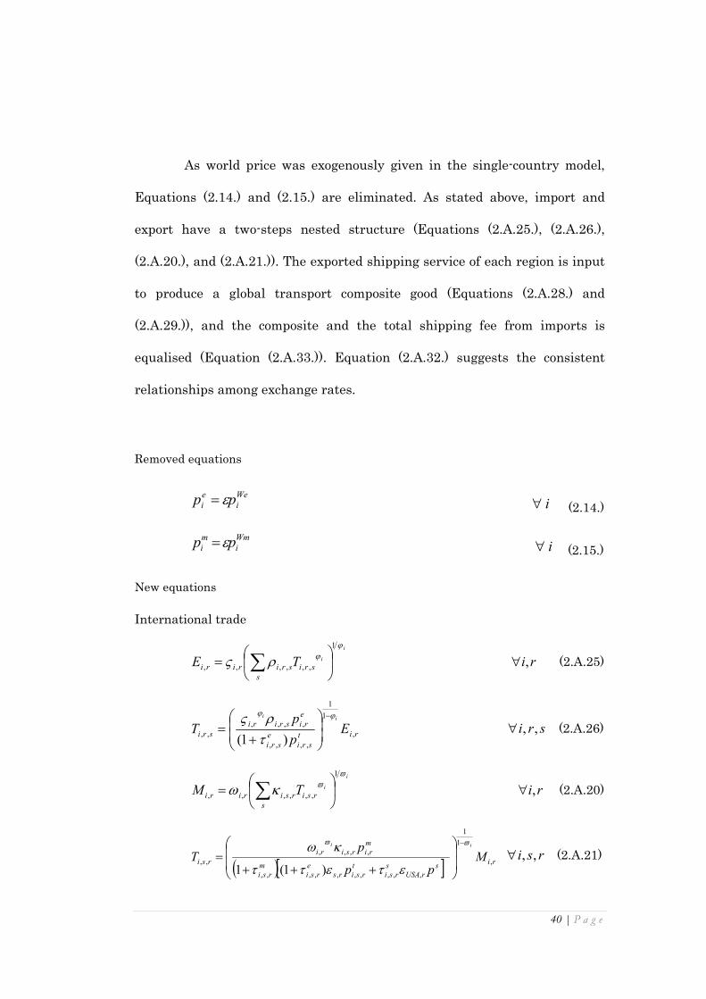
40 | P a g e

As world price was exogenously given in the single-country model,

Equations (2.14.) and (2.15.) are eliminated. As stated above, import and

export have a two-steps nested structure (Equations (2.A.25.), (2.A.26.),

(2.A.20.), and (2.A.21.)). The exported shipping service of each region is input

to produce a global transport composite good (Equations (2.A.28.) and

(2.A.29.)), and the composite and the total shipping fee from imports is

equalised (Equation (2.A.33.)). Equation (2.A.32.) suggests the consistent

relationships among exchange rates.

Removed equations

We

i

e

i pp ε= i∀ (2.14.)

Wm

i

m

i pp ε= i∀ (2.15.)

New equations

International trade

i

i

s

srisririri TE

ϕϕρς

1

,,,,,,

= ∑ ri,∀ (2.A.25)

rit

sri

e

sri

e

risriri

sri Ep

pT

ii

,

1

1

,,,,

,,,,

,,)1(

ϕϕ

τρς −

+= sri ,,∀ (2.A.26)

i

i

s

rsirsiriri TM

ϖϖκω

1

,,,,,,

= ∑ ri,∀ (2.A.20)

( )[ ] ris

rUSA

s

rsi

t

rsirs

e

rsi

m

rsi

m

rirsiri

rsi Mpp

pT

ii

,

1

1

,,,,,,,,,,

,,,,

,,

)1(1

ϖϖ

ετεττ

κω −

+++=

rsi ,,∀ (2.A.21)

41 | P a g e

Global transport sector

∏=r

r

s rTTcQχ

(2.A.28)

( )ss

z

rTRSUSAr

z

rTRS

rr Qp

pTT

,,,1 ετ

χ

+= r∀ (2.A.29)

∑=sri

sri

s

sri

s TQ,,

,,,,τ

(2.A.33)

Foreign exchange rate arbitrage condition

srsrrr ,,'', εεε =⋅ srr ,',∀ (2.A.32)

New Parameters

ri ,ζ : scale parameter of composite export transformation function

sri ,,ρ : share parameter of export

ri,ω : scale parameter of composite import production function

sri ,,κ : share parameter of import

Standard world CGE model equations

All the equations for the global CGE model explained in the previous

section are described below.

-Household

(Utility function: ∏=i

p

rir

ri

XUU,

,

α r∀ ) (2.A.1.)


42 | P a g e

−−= ∑ p

r

d

r

jh

rjh

f

rjhq

ri

rip

ri STFpp

X,

,,,,

,

,

,

α ri,∀ (2.A.2.)

Savings function

∑=jh

rjh

f

rjh

p

r

p

r FpsS,

,,,, r∀ (2.A.3.)

-Value added producing firm

Factor demand function

rjf

rjh

y

rjrjhrj

rjh Yp

pbF

vaj

vaj

,

1

1

,,

,,,,

,,

ηη β −

= rjh ,,∀ (2.A.4.)

Value added production function

vaj

vaj

h

rjhrjhrjrj FbY

ηηβ

1

,,,,,,

= ∑ rj,∀ (2.A.5.)

-Gross output producing firm

(Production function:

=rj

rj

irji

rji

rjay

Y

ax

XZ

,

,

,,

,,

, ,min rj,∀ ) (2.A.6.)

Demand function for intermediates

rjrjirji ZxX ,,,,, α= rji ,,∀ (2.A.7.)

Demand function for value added

rjrjrj ZayY ,,, = rj,∀ (2.A.8.)

Unit price function

y

rjrj

i

q

rirji

z

rj paypaxp ,,,,,, +=∑ rj,∀ (2.A.9.)

43 | P a g e

-Government

Demand function for government consumption

−++++= ∑∑∑∑ g

r

jh

f

rjh

sj

e

srj

sj

m

rsj

j

z

rj

d

rq

ri

rig

ri STTTTTp

X,

,,

,

,,

,

,,,

,

,

,

µ

ri,∀ (2.A.10.)

Direct tax revenue

rjh

jh

f

rjh

d

r

d

r FpT ,,

,

,,∑= τ r∀ (2.A.11.)

Production tax revenue

rj

z

rj

z

rj

z

rj ZpT ,,,, τ= rj,∀ (2.A.12.)

Import tariff revenue

( )[ ]rsj

s

rUSA

s

rsj

t

rsjrs

e

rsj

m

rsj

m

rsj TppT ,,,,,,,,,,,,,, 1 ετεττ ++= rsj ,,∀ (2.A.13.)

Export tax revenue

srj

t

srj

e

srj

e

srj TpT ,,,,,,,, τ= srj ,,∀ (2.A.14.)

Government savings function

++++= ∑∑∑∑

jh

f

rjh

sj

e

srj

sj

m

rsj

j

z

rj

d

r

g

r

g

r TTTTTsS,

,,

,

,,

,

,,,

r∀ (2.A.15.)

-Investment

Demand function for commodities for investment uses

( )frrUSA

g

r

p

rq

ri

riv

ri SSSp

X ,

,

,

, ελ

++= ri,∀ (2.A.16.)

-Armington composite good producing firm

Composite good production function

( ) iii

ri

d

riri

m

ririri DMQηηη δδγ1

,,,,,, += ri,∀ (2.A.17.)

Composite import demand function

rim

ri

q

ri

m

riri

ri Qp

pM

ii

,

1

1

,

,,,

,

ηη δγ −

= ri,∀ (2.A.18.)

44 | P a g e

Domestic good demand function

rid

ri

q

ri

d

riri

ri Qp

pD

ii

,

1

1

,

,,,

,

ηη δγ −

= ri,∀ (2.A.19.)

-Import variety aggregation firm

Composite import production function

i

i

s

rsirsiriri TM

ϖϖκω

1

,,,,,,

= ∑ ri,∀ (2.A.20.)

Import demand function

( ) ( )[ ] ris

rUSA

s

rsi

t

rsirs

e

rsi

m

rsi

m

rirsiri

rsi Mpp

pT

ii

,

1

1

,,,,,,,,,,

,,,,

,,

11

ϖϖ

ετεττ

κω −

+++=

rsi ,,∀ (2.A.21.)

-Gross output transforming firm

( ) iii

ri

d

riri

e

ririri DEZφφφ ξξθ

1

,,,,,, += ri,∀ (2.A.22.)

( )rie

ri

z

ri

z

ri

e

riri

ri Zp

pE

ii

,

1

1

,

,,,,

,

1 φφ τξθ −

+= ri,∀ (2.A.23.)

( )rid

ri

z

ri

z

ri

d

riri

ri Zp

pD

ii

,

1

1

,

,,,,

,

1 φφ τξθ −

+= ri,∀ (2.A.24.)

-Export variety producing firm

Composite export transformation function

i

i

s

srisririri TE

ϕϕρς

1

,,,,,,

= ∑ ri,∀ (2.A.25.)

Export supply function

rit

sri

e

risriri

sri Ep

pT

ii

,

1

1

,,

,,,,

,,

ϕϕ ρς −

= sri ,,∀ (2.A.26.)

45 | P a g e

Balance of payments

[ ] rsi

si

USAs

t

rsi

e

rsiUSAUSA

ss

rsi

r

z

rTRS

z

rTRSUSAr

f

rsri

t

sriUSAr

si

e

sri

Tpp

TTpSTp

,,

,

,,,,,,,,

,,,,,,,,

,

,,

)1(

)1()1(

∑

∑

++=

++++

ετετ

τεετ

r∀ (2.A.27.)

-Inter-regional shipping sector

Inter-regional shipping service production function

∏=r

r

s rTTcQχ

(2.A.28.)

Input demand function for international shipping service provided by the r-th

country

( )ss

z

rTRSUSAr

z

rTRS

rr Qp

pTT

,,,1 ετ

χ

+= r∀ (2.A.29.)

-Market-clearing conditions

Commodity market

∑+++=j

rji

v

ri

g

ri

p

riri XXXXQ ,,,,,, ri,∀ (2.A.30.)

Capital and land markets

∑=j

rjhrh FFF ,,, rh,∀ (2.A.31.)

Foreign exchange rate arbitrage condition

srsrrr ,,'', εεε =⋅ srr ,',∀ (2.A.32.)

Inter-regional shipping service market

∑=sri

sri

s

sri

s TQ,,

,,,,τ

(2.A.33.)

2.3.4 The modification of the standard CGE model for Chapter 3

Chapter 3 will discuss rice trade liberalisation policy by Japan. This

section describes how the standard world CGE model is changed for Chapter

46 | P a g e

3.

2.3.4.1 The Monte Carlo method9

While some countries call on Japan’s government to abolish the

import tariff on rice, the government has refused the proposal primarily on

the ground of its food security. Several papers have evaluated the impacts of

the rice free trade on its economy. Yet, most focus on the deterministic effects,

and therefore do not clearly answer whether the nation could secure its food

supply in an emergency after liberalisation. Chapter 3 will try to contribute

to this by assessing the probabilistic impacts of the rice trade liberalisation,

using an application of the Monte Carlo method taking into consideration the

rice productivity shocks of all the regions.

The Monte Carlo method is an approach to solve deterministic or

probabilistic mathematical problems using random numbers. Probabilistic

problems are simulations of a probabilistic phenomenon (or phenomena). In

the simulation, the elements are partly or entirely probabilistic, and the

probability of the events has to be specified. Deterministic problems are

where the problem is analytically solvable, but the equations are too complex

to solve or calculation efforts are enormous. The research in Chapter 3 is the

former classification and solves stochastic phenomena (possible welfare or

consumption changes of household) by generating random rice productivity

shocks.

9 This section explains the Monte Carlo method in general. For more information see Miyatake

and Nakayama (1960). Specific information on the method for this thesis will be described in

Chapter 3.

47 | P a g e

It originates from an idea by an American mathematician from

Poland, Stanislaw Marcin Ulam, who worked for the Los Alamos Laboratory

around 1946 (Metropolis and Ulam, 1949). It is said that Ulam was thinking

of the probability for finishing the card game “Solitaire.” The calculation

efforts are huge for the exponential increase in combination, but he realised

and told John von Neumann that the probability could be approximated by

randomly repeating the game, and that this method could also be applied to

explaining the diffusional phenomenon of the neutron in nuclear materials.

They devised the method of generating pseudo-random numbers on a

computer and so transforming a deterministic problem to a probabilistic

model.

As mentioned, an advantage of the Monte Carlo method is to make it

possible to approximate the solution of a problem that is not analytically

solvable. On the other hand, one of the disadvantages is not to be able to

avoid an error for a solution. Further, lots of experiments need to be

conducted for the high precision of estimation.

2.3.4.2 Productivity shocks parameter of paddy rice sector

In Chapter 3, a paddy rice productivity parameter is introduced into

a domestic rice production function (Equation (2.A.6.)), and thereby

Equations (2.A.7.), (2.A.8.) and (2.A.9.) are also transformed into Equations

((2.A.6.’), (2.A.7.’), (2.A.8.’) and (2.A.9.’)).

48 | P a g e

Equations after modification

=rj

rj

irji

rji

rjrjay

Y

ax

XTFPZ

,

,

,,

,,

,, ,min

rj,∀ (2.A.6.’)

rj

rjrji

rjiTFP

ZxX

,

,,,

,,

α= rji ,,∀ (2.A.7.’)

rj

rjrj

rjTFP

ZayY

,

,,

, = rj,∀ (2.A.8.’)

+= ∑ y

rjrj

i

q

rirji

rj

z

rj paypaxTFP

p ,,,,,

,

,

1 rj,∀ (2.A.9.’)

New exogenous variable

rjTFP, : productivity of j-th sector in r-th region (used only in rice

sector)

2.3.4.3 Emergency rice stock

Chapter 3 will also simulate the effectiveness of a rice buffer stock in

Japan. A rice stock variable is inserted into Equations (2.A.22.), (2.A.23.) and

(2.A.24.), which are replacing Equations (2.A.22.’), (2.A.23.’), and (2.A.24.’).

Equation (2.A.34.) expresses that rice stock is released into markets only

when a rice productivity shock is negative.

Equations after modification

( ) iii

ri

d

riri

e

ririrri DEEMSZφφφ ξξθ1

,,,,,, +=+ ri,∀ (2.A.22.’)

( ) ( )rrie

ri

z

ri

z

ri

e

riri

ri EMSZp

pE

ii

+

+=

−

,

1

1

,

,,,,

,

1 φφ τξθ

ri,∀ (2.A.23.’)

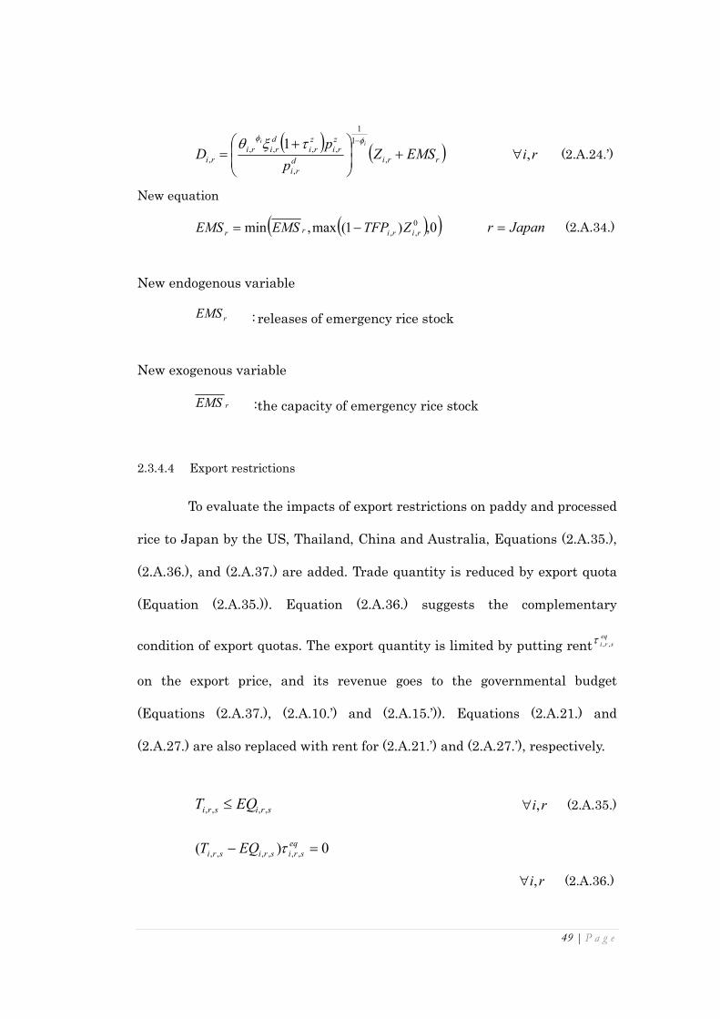
49 | P a g e

( ) ( )rrid

ri

z

ri

z

ri

d

riri

ri EMSZp

pD

ii

+

+=

−

,

1

1

,

,,,,

,

1 φφ τξθ

ri,∀ (2.A.24.’)

New equation

( )( )0,)1(max,min0

,, ririrr ZTFPEMSEMS −=

Japanr = (2.A.34.)

New endogenous variable

rEMS : releases of emergency rice stock


rEMS : the capacity of emergency rice stock

2.3.4.4 Export restrictions

To evaluate the impacts of export restrictions on paddy and processed

rice to Japan by the US, Thailand, China and Australia, Equations (2.A.35.),

(2.A.36.), and (2.A.37.) are added. Trade quantity is reduced by export quota

(Equation (2.A.35.)). Equation (2.A.36.) suggests the complementary

condition of export quotas. The export quantity is limited by putting renteq

sri ,,τ

on the export price, and its revenue goes to the governmental budget

(Equations (2.A.37.), (2.A.10.’) and (2.A.15.’)). Equations (2.A.21.) and

(2.A.27.) are also replaced with rent for (2.A.21.’) and (2.A.27.’), respectively.

srisri EQT ,,,, ≤ ri,∀ (2.A.35.)

0)( ,,,,,, =− eq

srisrisri EQT τ

ri,∀ (2.A.36.)

50 | P a g e

sri

t

sri

eq

sri

eq

sri TpT ,,,,,,,, τ= ri,∀ (2.A.37.)

−+++++= ∑∑∑∑∑ g

r

sj

eq

srj

jh

f

rjh

sj

e

srj

sj

m

rsj

j

z

rj

d

rq

ri

rig

ri STTTTTTp

X,

,,

,

,,

,

,,

,

,,,

,

,

,

µ

ri,∀ (2.A.10.’)

+++++= ∑∑∑∑∑

sj

eq

srj

jh

f

rjh

sj

e

srj

sj

m

rsj

j

z

rj

d

r

g

r

g

r TTTTTTsS,

,,

,

,,

,

,,

,

,,,

r∀ (2.A.15.’)

( ) ( )[ ] ris

rUSA

s

rsi

t

rsirs

eq

rsi

e

rsi

m

rsi

m

rirsiri

rsi Mpp

pT

ii

,

1

1

,,,,,,,,,,,,

,,,,

,,

11

ϖϖ

ετετττ

κω −

++++=

ri,∀ (2.A.21.’)

[ ] rsi

si

USAs

t

rsi

eq

sri

e

rsiUSAUSA

ss

rsi

r

z

rTRS

z

rTRSUSAr

f

rsri

t

sriUSAr

si

eq

sri

e

sri

Tpp

TTpSTp

,,

,

,,,,,,,,,,

,,,,,,,,

,

,,,,

)1(

)1()1(

∑

∑

+++=

+++++

εττετ

τεεττ

r∀ (2.A.27.’)

New endogenous variable

eq

sriT ,, : revenue from rent of export restrictions of i-th good from

r-th to s-th country

eq

sri ,,τ : rent of export restrictions of i-th good from r-th to s-th

country


sriEQ ,, : export quota of i-th good from r-th to s-th country

51 | P a g e

2.3.4.5 The structure of household consumption

The Cobb-Douglas form was applied to household consumption in the

standard model, but the empirical studies in Chapters 3, 4, 5 and 6 employ a

two-steps nested consumption structure for agricultural and food sectors with

a CES function (Figure 2.4).

Figure 2.4: the structure of household consumption for Chapter 3

A food composite is put into the utility function (Equation (2.A.1.’)), and

its demand function for food composite is derived (Equation (2.A.38)). The

food composite production function is the CES form (Equations (2.A.39.) and

(2.A.40.)).

Utility function for household

∏=nfd

p

rnfdrr

rnfdXFDr XXFDUU

,

,

αα

r∀ (2.A.1.’)


−−= ∑ p

r

d

r

jh

rjh

f

rjhq

rnfd

rnfdp

rnfd STFpp

X,

,,,,

,

,

,

α rnfd ,∀ (2.A.2.’)

−−= ∑ p

r

d

r

jh

rjh

f

rjhXFD

r

XFD

rr STFp

pXFD

,

,,,,

α r∀ (2.A.38.)

52 | P a g e

Food composite aggregation function

ΨΨ

∆Θ= ∑

1

,,

fd

p

rfdrfdrr XXFD r∀ (2.A.39.)

(Note that ff εε )1( −=Ψ .)

rq

rfd

XFD

rrfdrp

rfd XFDp

pX

Ψ−Ψ

∆Θ=

1

1

,

,

, rfd ,∀ (2.A.40.)

New set

fd : agricultural and food sectors

nfd : non-agricultural and food sectors

New endogenous variables

rXFD : food composite

XFD

rp : price of food composite

New parameters

XFD

rα : share parameter of a food composite

rΘ : scale parameter of food composite aggregate function

rfd ,∆ : share parameter of food composite function

fε : elasticity of substitution for food

Ψ : parameter related to elasticity of substitution for food

2.3.5 The modification of the standard CGE model for Chapters 4, 5 and 6

Like Chapter 3, the empirical research in Chapters 4, 5, and 6 will

53 | P a g e

employ a world model, part of which is modified from the standard model

shown above. The structure of household food consumption and the equations

for productivity shocks and export restrictions for Chapter 3 are used in

Chapters 4, 5 and 6 too. The new equations for these chapters are world oil

price and biofuel production. In addition, energy substitution structures are

put into both the firm production and the household consumption.

2.3.5.1 World oil price

oili =

{ }

{ } WOPwgtTp

wgtTp

r s

risri

t

sri

eq

sri

e

sri

o

iusar

r s

risri

t

sri

eq

sri

e

sri

o

iusar

∑ ∑

∑ ∑

+++=

+++

,,,,,,,,,,

,,,,,,,,,,

)1)(1(

)1)(1(

τττε

τττε

i∀ (2.A.41.)

∑ ++=si

sri

t

sri

eq

sri

e

sri

o

i

o

r TpT,

,,,,,,,, )1( τττ

r∀ (2.A.42.)

( ) ( )[ ] ris

rUSA

s

rsi

t

rsirs

eq

rsi

e

rsi

o

i

m

rsi

m

rirsiri

rsi Mpp

pT

ii

,

1

1

,,,,,,,,,,,,

,,,,

,,

1)1(1

ϖϖ

ετεττττ

κω −

+++++=

rsi ,,∀ (2.A.21.’’)

[ ] rsi

si

USAs

t

rsi

eq

sri

e

rsi

o

iUSAUSA

ss

rsi

r

z

rTRS

z

rTRSUSAr

f

rsri

t

sriUSAr

si

eq

sri

e

sri

o

i

Tpp

TTpSTp

,,

,

,,,,,,,,,,

,,,,,,,,

,

,,,,

)1)(1(

)1()1)(1(

∑

∑

++++=

++++++

ετττετ

τεετττ

r∀ (2.A.27.’’)


o

iτ : rent for world oil price

54 | P a g e

o

rT : revenue from oil price rent


WOP : world oil price control variable

New parameter

riwgt , : export weight

2.3.5.2 Biofuel production

To measure the impacts of the biofuel production increase in recent

years, the sector is subsidised to meet the production targets. In a similar

way to the export restriction equations, the domestic production is pushed up

by an exogenous variable rjPT , (Equation (2.A.43.)). Equation (2.A.44.) is the

complimentary condition for biofuel production. The expenditure is

considered in the governmental revenue (Equations (2.A.10.’’) and (2.A.15.’’)).

The changes are reflected in the supply functions of an export composite and

domestic good (Equations (2.A.23.’) and (2.A.24.’)).

rjrj PTZ ,, ≥

ri,∀ (2.A.43.)

0)( ,,, =− pt

rjrjrj PTZ τ

ri,∀ (2.A.44.)

rj

z

rj

pt

rj

pt

rj ZpT ,,,, τ=

ri,∀ (2.A.45.)

−−++++++= ∑∑∑∑∑∑ g

r

j

pt

rj

o

r

sj

eq

srj

jh

f

rjh

sj

e

srj

sj

m

rsj

j

z

rj

d

rq

ri

rig

ri STTTTTTTTp

X ,

,

,,

,

,,

,

,,

,

,,,

,

,

,

µ

ri,∀ (2.A.10.’’)

55 | P a g e

−++++++= ∑∑∑∑∑∑

j

pt

rj

o

r

sj

eq

srj

jh

f

rjh

sj

e

srj

sj

m

rsj

j

z

rj

d

r

g

r

g

r TTTTTTTTsS ,

,

,,

,

,,

,

,,

,

,,,

r∀ (2.A.15.’’)

( )rie

ri

z

ri

pt

ri

z

ri

e

riri

ri Zp

pE

ii

,

1

1

,

,,,,,

,

1 φφ ττξθ −

++= ri,∀ (2.A.23.’)

( )rid

ri

z

ri

pt

ri

z

ri

d

riri

ri Zp

pD

ii

,

1

1

,

,,,,,

,

1 φφ ττξθ −

++= ri,∀ (2.A.24.’)


pt

rj ,τ : subsidy rate of biofuel production target

pt

rjT , : subsidy of biofuel production target


rjPT , : biofuel production target

2.3.5.3 Energy substitution structure

Figures 2.5 and 2.6 indicate the structure of the model in Chapters 4, 5

and 6. Both the demand and supply sides have the same structure for energy

substitution. At the first stage, liquid energy goods such as oil are inputted to

produce a liquid energy composite good with a CES function (Equations

(2.A.49.), (2.A.50.), (2.A.56.) and (2.A.57.)), which is used to make an energy

composite with non-liquid energy goods like coal under the Cobb-Douglas

technology (Equations (2.A.46.), (2.A.47.), (2.A.53.), (2.A.54.) and (2.A.55.)).

With an energy composite good inserted as an intermediate good, the Leontief

56 | P a g e

domestic production function is transformed to Equation (2.A.6.’’), and its

demand function is derived (Equation (2.A.51.)). The household utility

function is also changed adding an energy composite good (Equation (2.A.1.’’)),

and its demand function is Equation (2.A.52.).

Figure 2.5: Model structure in Chapters 4, 5 and 6.

Figure 2.6: Model structure of household consumption in Chapters 4, 5 and 6.

57 | P a g e

Energy composite aggregation function

LQEC

rjXECrjnlq

rj

nlq

rjnlq

EC

rjrj LQXbEC_

,_,,

,,,,,

ββ×

= ∏ rj,∀ (2.A.46.)

rj

ec

rjq

rj

XEC

rjnlq

rjnlq ECpp

X ,,

,

_

,,

,,

β= rjnlq ,,∀ (2.A.47.)

rj

ec

rjlq

rj

LQEC

rj

rj ECpp

LQ ,,

,

_

,

,

β= rj,∀ (2.A.48.)

Liquid fuel composite aggregation function

h

h

/1

,,,,,,

= ∑

lq

rjlq

LQ

rjlq

LQ

rjrj XbLQ β rj,∀ (2.A.49.)

(Note that lqlq σσ )1( −=h .)

rjq

rjlq

lq

rj

LQ

rjlq

LQ

rj

rjlq LQp

pbX ,

1

1

,,

,,,,

,,

hh −

=

β rjlq ,,∀ (2.A.50.)

Gross output producing firm

(Production function:

=rj

rj

rj

rj

irjnen

rjnen

rjrjaec

EC

ay

Y

ax

XTFPZ

,

,

,

,

,,

,,

,, ,,min rj,∀ )

(2.A.6.’’)

rj

rjrj

rjTFP

ZaecEC

,

,,

, = rj,∀ (2.A.51.)

-Household

∏××=fd

p

rfdrrr

rfdECHr

XFDr XECHXFDUU

,

,

ααα r∀ (2.A.1.’’)

−−= ∑ p

r

d

r

jh

rjh

f

rjhech

r

ECH

rr STFp

pECH

,

,,,,

α r∀ (2.A.52.)

58 | P a g e

Energy composite aggregation function for household

×= ∏

LQHCr

ECHrnlq

r

nlq

p

nlq

ECH

rr LQHXbECH ββ ,

r∀ (2.A.53.)

r

ech

rq

rnlq

ECH

rnlqp

rnlq ECHpp

X,

,

,

β= rnlq,∀ (2.A.54.)

r

ech

rlqh

r

LQHC

rr ECHp

pLQH

β= r∀ (2.A.55.)

Liquid fuel composite aggregation function for household

ΞΞ

= ∑

/1

,,

lq

p

rlq

LQH

rlq

LQH

rr XbLQH β r∀ (2.A.56.)

(Note that lqhlqh σσ )1( −=Ξ .)

rq

rlq

lqh

r

LQH

rlq

LQH

rp

rlq LQHp

pbX

Ξ−Ξ

=

1

1

,

,

,

β rlq,∀ (2.A.57.)

New sets

lq : liquid energy goods

nlq : non-liquid energy goods


rECH : energy composite good for household

rLQH : liquid energy composite good for household

rjEC , : energy composite good

59 | P a g e

rjLQ , : liquid energy composite good

ec

rjp , : price of energy composite good

lq

rjp , : price of liquid fuel composite good

ech

rp : price of energy composite good for household

lqh

rp : price of liquid fuel for household

New parameters

EC

rjb , : scale parameter of energy composite production function

XEC

rjnlq

_

,,β : share parameter of a non-liquid energy good for energy

composite production function

LQEC

rj

_

,β : share parameter of a liquid energy composite for energy


LQ

rjb , : scale parameter of a liquid energy composite production

function

LQ

rjlq ,,β : share parameter of a liquid energy good for a liquid

energy composite production function

rjaec , : share parameter of an energy composite good for a

domestic production function

ECH

rα : share parameter of an energy composite good for a

household utility function

ECH

rnlq,β : share parameter of a non-liquid energy good for a

household’s energy composite production function

60 | P a g e

LQHC

rβ : share parameter of a liquid energy composite for a


ECH

rb : scale parameter of a household’s energy composite

production function

LQH

rlq,β : share parameter of a liquid energy good for a household’s

liquid energy composite production function

LQH

rb : scale parameter of a household’s liquid energy composite

production function

lqσ : elasticity of substitution of liquid energy goods

h : parameter related to elasticity of substitution of liquid

energy goods

lqhσ :elasticity of substitution of liquid energy goods for

household

Ξ : parameter related to elasticity of substitution of liquid

energy goods for household

2.4 Conclusion

We gave the basics of a SAM and CGE model, and showed our original

methods, models and the application of the Monte Carlo method for the thesis.

In the next chapter, we will apply the model to the topic of a rice free trade

problem in Japan in order to discuss its food security.

61 | P a g e

Appendix: list of variables and parameters

The endogenous variables, exogenous variables and parameters of the world

standard CGE model, the ones for the empirical studies in the thesis are

listed below.

World standard CGE model

Endogenous variables

p

riX , : household consumption

g

riX , : government consumption

v

riX , : investment uses

rjiX ,, : intermediate uses of the i-th good by the j-th sector

rjhF ,, : factor uses

rjY , : value added

rjZ , : gross output

riQ , : Armington composite good

riM , : composite imports

riD , : domestic goods

riE , : composite exports

sriT ,, : inter-regional transportation from the r-th region to the s-

th region

rTT : exports of inter-regional shipping service by the r-th

region

62 | P a g e

sQ : composite inter-regional shipping service

p

rS : household savings

g

rS : government savings

d

rT : direct taxes

z

rjT , : production taxes

m

rsjT ,, : import tariffs

e

srjT ,, : export taxes

f

rjhT ,, : factor input taxes

q

rip , : price of Armington composite goods

f

rjhp ,, : price of factors

y

rjp , : price of value added

z

rip , : price of gross output

m

rip , : price of composite imports

d

rip , : price of domestic goods

e

rip , : price of composite exports

t

srip ,, : price of goods shipped from the r-th region to the s-th

region

sp : inter-regional shipping service price in US dollars

63 | P a g e

sr ,ε : exchange rates to convert the r-th region’s currency into

the s-th region’s currency

Exogenous variables and parameters

f

rS : current account deficits in US dollars

rjhFF ,, : factor endowment initially employed in the j-th sector

0

,rjZ : initial amount of gross output

d

rτ : direct tax rates

z

ri ,τ : production tax rates

m

rsi ,,τ : import tariff rates on inbound shipping from the s-th

region

e

sri ,,τ : export tax rates on outbound shipping to the s-th region

s

sri ,,τ : inter-regional shipping service requirement per

unittransportation of the i-th good from the r-th region to

the s-th region

f

rjh ,,τ : factor input tax rates

Parameters

rjb , : scale parameter of production function for Yj

rjh ,,β : share parameter of factor input

f

jσ : elasticity of substitution for a value added composite

function

rjiax ,, : share parameter of intermediate input for domestic

64 | P a g e

production

rjay , : share parameter of composite factor input for domestic

production

va

jη : elasticity parameter

f

j

f

jva

j σ

ση

1+=

ri,θ : scale parameter of transformation function

ri,ξ : share parameter of transformation function

t

iσ : elasticity of transformation

iφ : parameter related to the elasticity of transformation

(t

i

i

t

i

i σ

σφ

1−=

)

ri,γ : scale parameter of Armington composite function

ri,δ : share parameter of Armington composite function

s

iσ : elasticity of substitution for an Armington function

iη : parameter related to the elasticity of substitution

(s

i

s

i

i σ

ση

1+=

)

ri ,ζ : scale parameter of composite export transformation

function

sri ,,ρ : share parameter of export

ri,ω : scale parameter of composite import production function

sri ,,κ : share parameter of import

65 | P a g e

ri,α : share parameter of household consumption

ri ,µ : share parameter of government consumption

ri,λ : share parameter of investment

p

rss : average propensity to save for household

p

rss : average propensity to save for government

Chapter 3


rXFD : food composite

XFD

rp : price of food composite

rEMS : release of emergency rice stocks

eq

sriT ,, : revenue from rent of export restrictions of i-th good from

r-th to s-th country

eq

sri ,,τ : rent of export restrictions of i-th good from r-th to s-th

country

Exogenous variables

rjTFP , : productivity; ( ) ( )0,1or,1~ 2

, NNTFP rrPDR σ

rEMS : capacity of emergency rice stocks

rσ : standard deviation of productivity in the paddy rice sector

sriEQ ,, : export quota of i-th good from r-th to s-th country

66 | P a g e

rjPT , : biofuel production target

Parameters

XFD

rα : share parameter of a food composite

rΘ : scale parameter of food composite aggregate function

rfd ,∆ : share parameter of food composite function

fε : elasticity of substitution for food

Ψ : parameter related to elasticity of substitution for food

riwgt , : export weight

Chapters 4, 5, and 6


pt

rj ,τ : subsidy rate of biofuel production target

pt

rjT , : subsidy of biofuel production target

rECH : energy composite good for household

rLQH : liquid energy composite good for household

rjEC , : energy composite good

rjLQ , : liquid energy composite good

ec

rjp , : price of energy composite good

lq

rjp , : price of liquid fuel composite good

ech

rp : price of energy composite good for household

67 | P a g e

lqh

rp : price of liquid fuel for household

Parameters

EC

rjb , : scale parameter of energy composite production function

XEC

rjnlq

_

,,β : share parameter of a non-liquid energy good for energy


LQEC

rj

_

,β : share parameter of a liquid energy composite for energy


LQ

rjb , : scale parameter of a liquid energy composite production

function

LQ

rjlq ,,β : share parameter of a liquid energy good for a liquid

energy composite production function

rjaec , : share parameter of an energy composite good for a

domestic production function

ECH

rα : share parameter of an energy composite good for a

household utility function

ECH

rnlq,β : share parameter of a non-liquid energy good for a


LQHC

rβ : share parameter of a liquid energy composite for a


ECH

rb : scale parameter of a household’s energy composite

production function

LQH

rlq,β : share parameter of a liquid energy good for a household’s

liquid energy composite production function

68 | P a g e

LQH

rb : scale parameter of a household’s liquid energy composite

production function

lqσ : elasticity of substitution of liquid energy goods

h : parameter related to elasticity of substitution of liquid

energy goods

lqhσ : elasticity of substitution of liquid energy goods for

household

Ξ : parameter related to elasticity of substitution of liquid

energy goods for household

69 | P a g e

3 Does agricultural trade liberalisation increase risks of

supply-side uncertainty?: Effects of productivity shocks

and export restrictions on welfare and food supply in

Japan

3.1 Introduction

The agricultural sector in developed countries has been the central

target of reform in multilateral trade negotiations led by the World Trade

Organization (WTO) and bilateral free trade arrangements. Japan did not

have an active role in those negotiations, although the benefits of free trade

were immense as suggested by, for example, Anderson et al. (2006). The

interested parties in Japan—farmers, politicians, and the Japanese

Government, more specifically the Ministry of Agriculture, Forestry, and

Fisheries (MAFF)—have called for protection and exceptional treatment for

this sector, particularly for rice farming, every time new trade negotiations

have been launched. Their arguments are twofold. One is the

“multifunctionality” of the agricultural sector, which appreciates the

(positive) externalities of agricultural activities such as protection of natural

environments, rural scenery, culture, and so on, studied by the Science

Council of Japan (2001). The other reason, discussed here, is “national food

security”—concerning uncertainty in the food supply, which can be

jeopardized by unforeseen supply-side shocks such as bad crops, war, and

70 | P a g e

embargoes.1 The MAFF stresses the promotion of domestic production to

secure food supply, which is often subject to these risk factors, while

considering importation as a secondary source, as the Basic Law on Food,

Agriculture and Rural Areas (the Basic Law, hereinafter) states.

The concern about food supply sounds like a reasonable justification

for protection in an age of uncertainty, considering the fact that Japan’s food

self-sufficiency rate is a mere 40%, measured on the basis of calories, which is

a significantly lower rate than those of other major developed countries.

While this low food self-sufficiency rate is a result of the outstanding

comparative advantage of Japan’s industrial sectors, it can make the

Japanese economy susceptible to food shortages caused by the

aforementioned shocks. In fact, bad weather in 1993 reduced the country’s

rice harvest by 26% compared with the average yield, the second worst year

on record since 1926.2 There was a soybean export embargo because of a

serious crop failure in the US in 1973 and a grain export embargo in response

to the USSR’s invasion of Afghanistan in 1980.

1 The focus of Japan’s national food security is slightly different from that of the popular

concept of food security. The former is set on food security in contingency in the developed

economy of Japan, the latter on food security in developing economies, which are vulnerable

to shocks because of their continuing poverty in the short run and poor capability of feeding

rapidly growing populations in the long run. Hayami (2000) discussed their difference in

detail.

2 The worst decline of 33% occurred in 1945.

71 | P a g e

3.1.1 National food security and Japan’s agricultural policy

Excessive dependency on imports for food supply is considered a risk

factor for Japan’s national food security. MAFF (2006) established a

contingency plan to secure food supplies for domestic consumption in

emergencies. This plan was put into place to achieve national food security as

defined in the Basic Law, which had been revised the year before. MAFF

defined 2,000 kcal/person/day (about 20% less than usual) as the minimum

calorie intake. The plan included several measures to secure the calorie

intake, such as promoting domestic production, managing emergency stocks,

and controlling food markets. Among the crops, rice has been the most

important commodity for Japan. In 2004, rice comprised 23% of the

population’s total calorie intake, followed by wheat, which contributed 13% of

the total. The government keeps large emergency stocks of rice and other

major crops to secure the food supply, while making continuing efforts to

increase the country’s food self-sufficiency rate.

High trade barriers on rice have played an important role in the

achievement of an almost 100% of self-sufficiency rate for rice. Proponents of

these trade barriers argue that they are necessary to maintain the overall

self-sufficiency rate of food because the supply of other foods depends heavily

on imports. Even though trade theories imply gains from trade, proposals for

free rice trade have never been accepted in Japan because free trade lowers

the food self-sufficiency rate, and thereby increases the dependency of the

food supply on imports, which is supposed to make the food supply less secure.

The impact of agricultural trade liberalisation is twofold: (1)

72 | P a g e

deterministic gains from trade achieved through the removal of trade

barriers and (2) stochastic gains and losses caused by productivity shocks,

whose magnitude can be exacerbated or mitigated depending on the level of

trade openness. Researchers have often analysed the first aspect of trade

liberalisation but have rarely examined the second aspect. This lack of

analysis of the second aspect leads to people being uninformed and triggers

their opposition to trade liberalisation, simply because trade liberalisation is

generally believed to make the domestic economy susceptible to shocks from

abroad.

3.1.2 The rice trade and its barriers

Japan has previously strictly prohibited imports of rice but permitted

minimum access (MA) imports of rice in 1995 and their tariffication in 1999

as a part of the GATT Uruguay Round agreement. The imports account for

only 10% of domestic production because of prohibitively high trade barriers.

If these trade barriers are abolished, imports are expected to have a very high

share in the total rice supply as suggested by previous studies, for example,

Cramer et al. (1993) and Wailes (2005).

Japan’s rice consumption is comprised mainly of mid- or short-grain

rice (so-called japonica rice), rather than long-grain rice (indica rice). The

former is strongly preferred in East Asian countries while the latter type is

popular elsewhere in Asia and in other regions. Japan’s rice trade patterns

reflect this preference. Japan’s three major rice trade partners (China, the

US, and Australia) produce japonica rice and expect to increase their exports

73 | P a g e

to Japan after the rice trade is liberalised.

As rice in many countries is mainly produced and consumed

domestically, its international trade is thin. Only a small fraction of

production is exported and imported internationally unlike wheat, maize, and

so on. The top 10 rice producing countries, many of which are in Asia, cover

almost 90% of the world’s total production of rice. Their production fluctuates

with weather conditions, including droughts, cool summer days, and

cyclones/typhoons. While productivity has an upward-sloping trend, it

sometimes shows sudden drops (see Figure 3.1).

Figure 3.1: Productivity fluctuations of paddy rice [Unit: tons/hectare]

Data source: FAOSTAT

Once Japan’s rice market is liberalised, any shocks in the domestic

and foreign markets will directly affect its food supply. Furthermore, taking

0

1

2

3

4

5

6

7

8

9

10

1990

1992

1994

1996

1998

2000

2002

2004

2006

2008

Japan

China

India

Indonesia

Bangladesh

Vietnam

Thailand

Philippines

US

Australia

Rest of Asia

Other countries

74 | P a g e

into account Japan’s strong preference towards japonica rice, the

international market seems much less reliable as an alternative supply

source. Therefore, it might seem a reasonable idea that national food security

can only be established by protecting the domestic rice market in order to

maintain the self-sufficiency rate of food, rather than by depending on foreign

supply sources.

3.1.3 Literature review

The majority of existing studies on Japan’s rice trade liberalisation

have been conducted from a deterministic viewpoint. Cramer et al. (1999)

developed a 22-country world rice trade model and found that Japan would

import three million tons of rice (about one-third of domestic consumption)

with an 8% annual tariff reduction after tariffication. In their conclusion,

they suggested that food security could be improved by increasing

accessibility to international markets, rather than through protection.

However, they did not explicitly consider whether the international markets

could be reliable, considering fluctuating productivity inside and outside of

Japan.

Using a spatial equilibrium model, Cramer et al. (1993) found that

the removal of direct and indirect rice trade barriers in all countries would

lead to increases in Japan’s rice imports by about five million tons. Wailes

(2005) conducted a similar but updated analysis on the elimination of tariffs

and export subsidies and found that the increase in rice imports would be

about two million tons. Overall, these results indicate that free rice trade

75 | P a g e

would lead to imports into Japan constituting as much as 20–50% of domestic

consumption. Through these imports, foreign-made shocks would affect the

Japanese economy.

On the other hand, there are only a few studies that have examined

agricultural trade liberalisation from the view of national food security. Hosoe

(2004) developed a world trade computable general equilibrium (CGE) model

to evaluate the impact of Japan’s domestic productivity shock in 1993 on its

own economy under rice price controls and the impact of Japan’s emergency

rice imports on other countries. The productivity shock was assumed to be

deterministic in the sense that its magnitude was calibrated to reproduce

that historical event in 1993. Most recently, Maeda and Kano (2008)

examined the effect of an international rice reserve system to stabilise rice

markets, using a spatial equilibrium model that considered fluctuating rice

supplies using a Monte Carlo simulation method.

In this study, we ask whether it is reasonable to sacrifice gains from

trade for the sake of national food security, to what extent rice supply can be

secured by its stockpile, and whether Japan, as one of the world’s largest

economic powers, is likely to suffer from food shortages as discussed by

Hayami (2000). To this end, we develop a world trade CGE model in

combination with a Monte Carlo simulation method that provides a

comprehensive framework to analyse international rice markets under

uncertainty. We take into account risk factors such as low food self-sufficiency

induced by trade liberalisation, and a wide range of productivity shocks

inside and outside of Japan. This technique is similar to that used by Harris

76 | P a g e

and Robinson (2001) to analyse the impact of weather fluctuations induced by

El Niño on regional agricultural output and income distribution in Mexico.

We also evaluate the effectiveness of the Japanese government’s emergency

stocks, held in preparation for a crop failure. Moreover, we simulate rice

export quotas set by major rice exporters to Japan. By using a CGE model,

we can depict how these shocks breaking out in the rice sector affects the

macroeconomy and how rice is substituted with other foods to mitigate the

impact of the shock.

This chapter proceeds as follows. We explain our world trade CGE

model in Section 2 and simulation scenarios in Section 3. Simulation results

are presented in Section 4. Our conclusions are provided in Section 5. In the

appendix of this chapter we further report the relevant sensitivity analyses.

3.2 Structure of the world trade CGE model

While using the basic structure of the single-country CGE model

described by Devarajan et al. (1990), we extend the model to create a

multicountry model to analyse international rice markets under uncertainty.

Reflecting the fact that Japan’s rice trading partners are mostly Asia-Pacific

countries, we distinguish 12 regions using the Global Trade Analysis Project

(GTAP) database (version 7.1).3 Each region has eight sectors, including five

food-related sectors (Table 3.1). Each sector is represented by a perfectly

competitive profit-maximizing firm with a Leontief production function for

3 For more information about the GTAP database, see Hertel (1997).

77 | P a g e

gross output and with a constant elasticity of substitution (CES) production

function for value-added components (Figure 2.3). For the elasticity of

substitution, we assume 0.2 for the agricultural sectors (paddy rice, wheat,

and other agriculture) and 1.0 for the other sectors.4 Among the value-added

components, capital is assumed to be immobile among sectors in order to

model relatively short-run phenomena under unforeseen shocks in all

simulations (except Scenario M, discussed later) presuming a situation where

productivity shocks are observed after allocation of capital has been

determined.5 In contrast, labour is assumed to be mobile among sectors.

International factor mobility is not assumed. These factors are assumed to be

fully employed with flexible factor price adjustments.

4 Even when we alternatively assume 0.1 or 1.0 for this elasticity in these agricultural sectors,

our conclusions are found to be almost qualitatively robust. Details are shown in the

appendix.

5 When we alternatively assume all the factors are mobile, Japan and other countries can

absorb such shocks more flexibly and experience smaller welfare fluctuations. This

alternative assumption reinforces rather than undermines the robustness of our conclusions.

78 | P a g e

Table 3.1: List of regions and sectors in the model

Note: Asterisks indicate food commodities used for the food composite.

Sectoral gross outputs are split into domestic outputs and composite

exports using a constant elasticity of transformation (CET) function. The

domestic goods and composite imports are aggregated into composite goods

using a CES function as assumed by Armington (1969). The composite

imports consist of imports from various regions, and the composite exports

are decomposed into exports to various regions. For these CES/CET functions,

we use the elasticity of substitution as suggested in the GTAP database. The

elasticity of substitution represents the similarity of goods differentiated by

the origin and destination of trade. For example, the elasticity of substitution

between the domestic goods and the composite imports is assumed to be 5.05

for paddy rice and 2.60 for processed rice.6 With this nested CES structure,

6 We assume no active stock behaviour except in the case considering Japan’s emergency

stocks in scenario S, discussed later.

Region Sector

Japan Paddy rice*

China Wheat*

India Other agriculture*

Indonesia Processed rice*

Bangladesh Other food*

Vietnam Manufacturing

Thailand ServicesPhilippines TransportationUSAustraliaRest of Asia

Other countries

79 | P a g e

we can describe how rice trade liberalisation lowers import prices leading to

the substitution of domestic production by foreign rice. We can also describe

how shocks inside and outside Japan are propagated through the

international rice trade.

Although we do not explicitly control for the different types of rice

grains in our model, the nested CES structure approximately reflects Japan’s

preference for japonica rice. Share parameters in the CES functions are

calibrated in order to reproduce the actual trade flows of rice, mainly from

countries that produce japonica rice. Exchange rates are flexibly adjusted so

that the current account balance remains constant in US dollar terms in all

regions.

Composite goods are used for consumption by the household, as well

as for government, investment, and intermediate input.7 If the commodity is

one of the food commodities listed in Table 3.1, it is aggregated into a food

composite along with other food commodities. The food composite contributes

to utility (Figure 2.4). This structure describes substitution among foods in

household consumption with a CES function, which gives flexibility to our

assumptions about the price elasticity of food consumption demand.

Surveying existing literature, we assume that its elasticity of substitution is

0.1.8 If the commodity is not a food, it contributes directly to utility.9

7 See footnote 6.

8 Generally, the price elasticity of necessities like rice is supposed to be very small. However,

there is a variety of rice price elasticity estimates ranging from zero or 0.1 to 2.8. A survey of

these parameter estimates and a sensitivity analysis with respect to this elasticity are

80 | P a g e

3.3 Simulation scenarios

To quantify the welfare impact of Japan’s rice trade liberalisation on

the country’s national food security, we conduct comparative static analyses

considering the following scenario factors: (1) unilateral abolition of trade

barriers on paddy and processed rice imports by Japan; (2) fluctuations of

productivity in the paddy rice sector; (3) emergency stocks to mitigate the

adverse impact of anticipated productivity shocks; and (4) quotas on rice

exports imposed by the four major rice exporters to Japan. We set up 11

scenarios to determine the extent to which Japan’s national food security is

jeopardized or ensured by these scenario factors identified in Table 3.2.

provided in the appendix. Our simulation results are also found to be qualitatively robust in

this sensitivity analysis.

9 The complete list of model equations is provided in the annex.

81 | P a g e

Table 3.2: Scenario design

The first two scenarios, T0 and T1, are conventional ones used to

assess deterministic gains from trade. As no shock is assumed in Scenario T0

as a base run, its results are nothing but the original GTAP data. The six

subsequent scenarios are used to investigate the impact of trade

liberalisation on regimes subject to productivity shocks in Japan (Scenarios

J0 and J1), the rest of the world (Scenarios R0 and R1), and all over the world

(Scenarios A0 and A1). Scenario S is used to analyse the effectiveness of the

government stocks. The last two Scenarios M and Q are used to evaluate the

impact of possible export quota impositions by rice exporters. Details of those

scenario factors are provided below.

3.3.1 Scenario factor 1: Abolition of trade barriers

We assume unilateral abolition of tariff and nontariff barriers by

Japan which are reported by the GTAP database. The tariff rates and tariff-

equivalent trade barriers on paddy and processed rice imports generally

T0 – – – – – –T1 x – – – – –R0 – – x – – –R1 x – x – – –J0 – x – – – –J1 x x – – – –A0 – x x – – –

A1 x x x – – –S – x x x – –M x – – – x –Q x – – – – x

Capitalmobility

Tradelibera-

lization

Shocks inRice

stocksJapanRest of

the world

Exportquotas

Scenario

82 | P a g e

reach several hundred percent. Neither border barriers in the other sectors

nor those in the other regions are changed.

3.3.2 Scenario factor 2: Productivity shocks

We assume that productivity shocks happen randomly to the total

factor productivity parameter of the gross output production function in the

paddy rice sector, following the independent identically distributed normal

distribution ( )2,1 rN σ for region r. We measure the productivity of the paddy

rice sector by production per acre of harvested area and estimate the

standard deviations rσ of the productivity of these 12 regions with time

series data for 15 years (1990–2004) provided by FAOSTAT, while removing

the effect of the time trend on productivity (Table 3.3).10 We simulate 1,000

Monte Carlo draws for each scenario. Among our 1,000 draws, Australia

shows the worst maximum productivity decline (26% compared with the

mean yield) among the 12 regions, followed by Japan. In the other regions,

maximum productivity declines are about 10–20%.

10 The estimated residuals do not seem spatially correlated by simple examination using a

correlation matrix. Even if we assume a doubling of the standard deviations for productivity

in all the regions for our simulations, we find our conclusions qualitatively robust in general.

Results are summarized in the appendix and the annex.

83 | P a g e

Table 3.3: Regression results of paddy rice productivity

[Dependent variable: rice productivity index (2001=1.00)]

Note: T-values are in parentheses. * and ** indicate parameters are

significant at 10% and 5% significance levels, respectively.

Means (=1.00) and standard deviations (SD) of the Monte Carlo draws are all

consistent with those of the original estimates for the residuals.

When an adverse productivity shock takes place in Japan—whose

domestic output is almost only for domestic use—the country’s domestic

consumption is reduced but is supported partly by imported rice. Similarly,

when an abundant rice crop is harvested in Japan, the surplus can be

Min. Max.Japan –9.7352 0.0053 0.0801 0.088 0.75 1.31

(–1.02) (1.12)China –12.9460 0.0070 0.0261 0.606 0.91 1.08

(–4.16)** (4.47)**

India –15.6576 0.0083 0.0423 0.453 0.87 1.16(–3.1)** (3.28)**

Indonesia –4.2802 0.0026 0.0186 0.304 0.94 1.07(–1.93)* (2.38)**

Bangladesh –47.7156 0.0243 0.0467 0.854 0.84 1.13

(–8.57)** (8.73)**Vietnam –54.6946 0.0278 0.0159 0.985 0.95 1.05

(–28.85)** (29.33)**Thailand –35.8382 0.0184 0.0295 0.893 0.89 1.10

(–10.17)** (10.43)**Philippines –22.8654 0.0119 0.0502 0.548 0.83 1.16

(–3.82)** (3.97)**US –26.4873 0.0137 0.0366 0.752 0.86 1.11

(–6.07)** (6.28)**

Australia –5.9156 0.0034 0.0885 0.031 0.74 1.25(–0.56) (0.65)

–19.6074 0.0103 0.0212 0.836 0.94 1.07(–7.76)** (8.14)**

–33.3938 0.0172 0.0228 0.924 0.93 1.08

(–12.26)** (12.6)**

Regression results of paddy rice productivity Monte Carlo draws

Intercept Time trendSD of

residualsR

2

Rest of Asia

Other

countries

84 | P a g e

absorbed abroad. Under a freer rice trade regime, Japan can access

international rice markets more easily and manage shocks to its domestic

production through imports more flexibly. In view of the statistical

distribution of domestic welfare, given the same magnitude of productivity

shocks, trade liberalisation itself shifts the mean of the welfare distribution

upwards and decreases the standard deviation of the welfare distribution (the

upper graph of Figure 3.2). In this case, whether a productivity shock is

negative or positive, trade liberalisation always brings about a preferable

impact on welfare distribution.

Figure 3.2: Impact of productivity shocks and trade liberalisation on

distribution of Japan’s welfare

In contrast to these cases with productivity shocks in Japan, when an

85 | P a g e

adverse productivity shock takes place in the rest of the world, particularly in

China, the US, or Australia, Japan’s imports from these countries are

jeopardized. As protectionists warn, rice trade liberalisation increases Japan’s

dependency on imported food and thus can exacerbate the impact of adverse

productivity shocks on Japan. However, if a positive productivity shock takes

place in those countries, Japan can conversely gain by the same mechanism.

As the productivity parameter, by definition, is distributed around its mean,

such productivity shocks as a whole do not seriously deteriorate the mean of

the welfare distribution in Japan. Instead, they increase the standard

deviation of the welfare distribution while trade liberalisation brings

deterministic gains through improvements of efficiency in resource allocation

(the lower graph of Figure 3.2). In this case, without combining the impact of

trade liberalisation with those of productivity shocks on the distribution of

welfare, we cannot judge immediately whether trade liberalisation is always

welfare improving.

3.3.3 Scenario factor 3: Emergency stocks

Preparing emergency stocks is a popular measure used for coping

with bad crops. The impact of the rice supply shock in 1993 was exacerbated

partly by the government-led restructuring of Japan’s food system. The

government had significantly reduced its rice stocks to 0.23 million tons,

covering 2.5% of consumption in a normal year. After the bad harvest in 1993,

the government increased the size of the emergency stocks to 1.5 million tons,

equivalent to 17% of the annual production in 2004. We assume this stock is

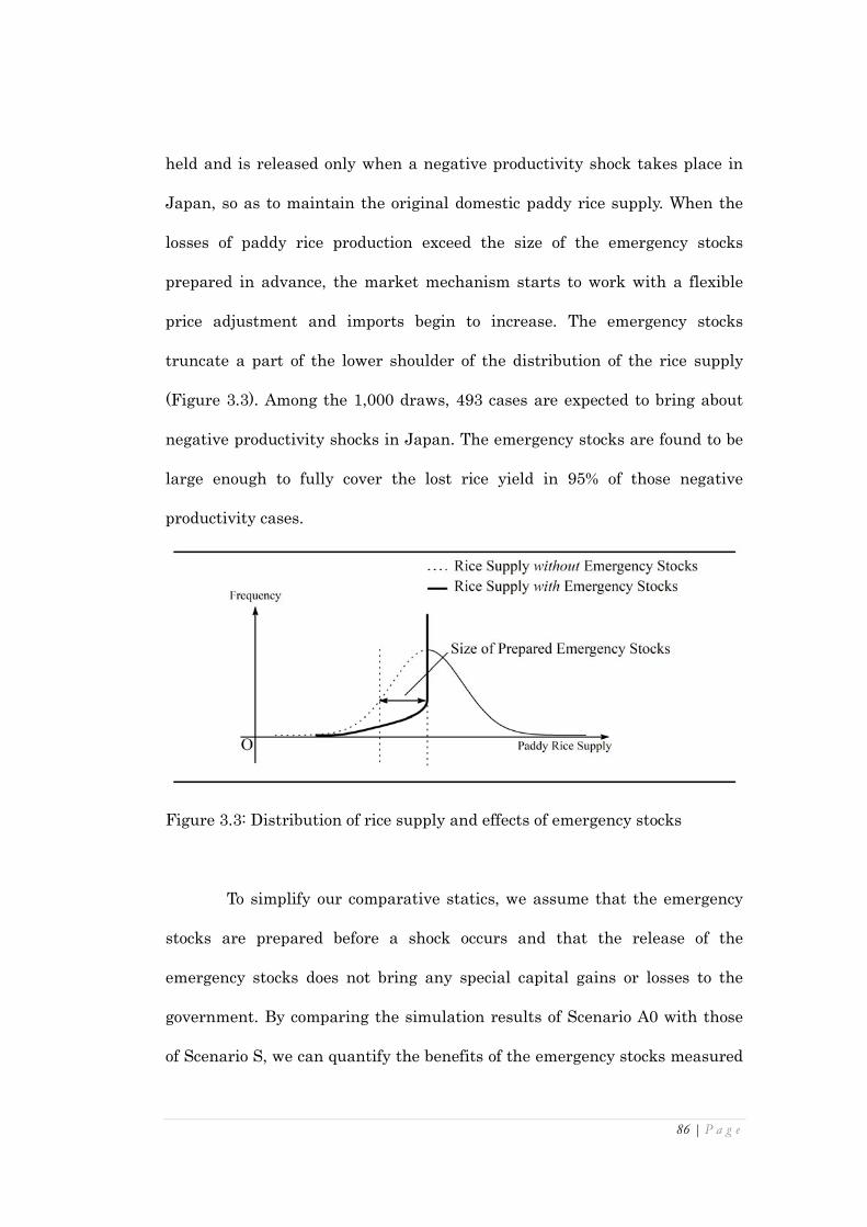
86 | P a g e

held and is released only when a negative productivity shock takes place in

Japan, so as to maintain the original domestic paddy rice supply. When the

losses of paddy rice production exceed the size of the emergency stocks

prepared in advance, the market mechanism starts to work with a flexible

price adjustment and imports begin to increase. The emergency stocks

truncate a part of the lower shoulder of the distribution of the rice supply

(Figure 3.3). Among the 1,000 draws, 493 cases are expected to bring about

negative productivity shocks in Japan. The emergency stocks are found to be

large enough to fully cover the lost rice yield in 95% of those negative

productivity cases.

Figure 3.3: Distribution of rice supply and effects of emergency stocks

To simplify our comparative statics, we assume that the emergency

stocks are prepared before a shock occurs and that the release of the

emergency stocks does not bring any special capital gains or losses to the

government. By comparing the simulation results of Scenario A0 with those

of Scenario S, we can quantify the benefits of the emergency stocks measured

87 | P a g e

with a welfare indicator. In addition, by subtracting the storage costs of the

emergency stocks from the benefits, we can see the net benefits of the

emergency stocks.

3.3.4 Scenario factor 4: Export quotas

While productivity shocks jeopardize both the domestic and the

foreign rice supply every year, export quotas damage Japan by limiting the

foreign supply. In designing scenarios for the quota analysis, we need some

reconsideration of the reference equilibrium, which describes the status quo.

If we simulate export quotas based simply on the reference equilibrium that

is characterized by the abundant domestic rice production capacity and the

very low penetration of foreign rice (i.e., Scenario T0), it is obvious that the

impact of quota imposition should be negligibly small. We cannot derive any

significant implications from such a simulation analysis.

In reality, the damage from export quotas is serious when Japan has

substituted imported rice for domestic rice under the free rice trade regime

and has reduced its domestic production capacity by reallocating factors

(particularly capital) away from the paddy rice sector in the long run.

Especially for this quota analysis, this situation is computed by assuming rice

trade liberalisation with inter-sectoral mobility of all the factors and defining

a new reference equilibrium—let it be referred to as the intermediate

equilibrium (Scenario M). Then, we assume no inter-sectoral mobility of

capital and simulate export quotas set by the four major rice exporters,

Australia, China, Thailand, and the US, to Japan (Scenario Q). The size of

88 | P a g e

the export quota is assumed to be as large as the original import level from

these exporters described in Scenario T0.

3.4 Simulation results

We simulate random productivity shocks and various policies and

quantify the costs and benefits of trade liberalisation for the Japanese

economy. The simulation results are summarized in Table 3.4 and presented

graphically in Figure 3.4.

Table 3.4: Summary statistics of simulation results for Japan

Calorie

intake

Self-suff.

rate of rice

Min. Mean Max. SD % of GDP Mean SD Min. Mean

Mean/GDP [base=1.00][kcal/person

/day][%]

T0 – 0 – – 0.00 1.00 – 2,564 94.2

T1 – 4,453 – – 0.10 0.28 – 2,622 62.4

R0 –102 0 94 26 0.00 1.01 0.04 2,562 94.2

R1 4,202 4,454 4,710 69 0.10 0.28 0.01 2,619 62.4

J0 –8,358 –319 3,515 1609 -0.01 1.00 0.01 2,474 93.7

J1 1,561 4,371 6,589 707 0.10 0.28 0.00 2,602 62.1

A0 –8,216 –319 3,518 1609 -0.01 1.01 0.04 2,476 93.7

A1 1,711 4,371 6,558 710 0.10 0.28 0.01 2,603 62.1

S –6,019 –57 3,518 1229 0.00 1.00 0.02 2,521 91.5

M – 5,707 – – 0.13 0.29 – 2,611 36.0

Q – –15,340 – – -0.34 1.20 – 2,334 46.8

Scenario

Welfare (EV)

[mil. US$]

Import price of

processed rice

89 | P a g e

Figure 3.4: Distribution of Japan’s welfare [Unit: EV in millions of US

dollars]

3.4.1 Deterministic impact of trade liberalisation

When we assume abolition of all the tariff and nontariff barriers on

paddy and processed rice imports by Japan (Scenario T1), imports of paddy

and processed rice surge to reduce Japan’s paddy rice production by 30%

90 | P a g e

compared with Scenario T0.11 Rice consumption is increased by 8% because of

consumers exploiting the falls in rice prices. As a result, the overall welfare

gains measured by equivalent variations (EV) are US$4,453 million.

3.4.2 Productivity shocks in the rest of the world

People are often concerned that when they are heavily dependent on

foreign supply sources for rice, the food supply could be insecure because of

unforeseen productivity shocks in other countries. A comparison of results

between Scenarios R0 and R1 indicates whether these concerns are

reasonable or just imaginary. The results of Scenario R0 show no change from

those of Scenario T0 in the mean of Japan’s welfare distribution, but do show

some change in its volatility.12 The welfare distribution of Scenario R0 (and

11 The increase of japonica rice imports by Japan has to be consistent with export capacity of

the four major rice exporters, particularly China, where japonica rice is not produced in large

quantities. We do not distinguish among the various rice types in our model or consider

exporters’ supply capacities of japonica rice, but approximate Japan’s preference toward

japonica rice and exporters’ japonica rice supply capacity with the nested CES/CET structure.

Thus, it is difficult to examine the validity of our model and results directly. In this regard,

the simulation results of other studies where several rice types were distinguished may help

us to estimate China’s export supply capacity of japonica rice. For example, Cramer et al.

(1993) predicted that trade liberalization would cause China to significantly increase exports

of both indica and japonica rice by 6–7 million tons in total, where japonica would comprise

about 35–40% of its total exports. A similar finding was reported by Wailes (2005).

12

The mean of the welfare impact is found to be slightly negative in scenarios J0 and A0,

where we assume only productivity shocks. This is because of the concavity of the utility

91 | P a g e

Scenarios J0 and A0, discussed later) indicates that without liberalising rice

imports there is no statistically significant chance for Japan to attain the

deterministic gain achieved in Scenario T1.

Abolition of trade barriers on rice imports increases the penetration

of foreign rice, which is subject to productivity shocks. The results of Scenario

R1 show that trade liberalisation increases both the mean and the standard

deviation of welfare compared with those of Scenario R0. This increase in

volatility is, however, not so large that it brings a case for Japan to suffer

negative welfare impact among the 1,000 cases. Furthermore, the worst

welfare level (US$4,202 million) achieved under free rice trade (Scenario R1)

is far better than the best welfare level (US$94 million) without free rice

trade (Scenario R0).

The impact of productivity shocks in foreign countries can be

confirmed by examining import prices for Japan. While rice trade

liberalisation lowers the import price of processed rice by about 70% on

average, its price fluctuations seem to be almost nil. Therefore, the

productivity shocks abroad do not cause any price hikes or adversely affect

household rice consumption.

3.4.3 Productivity shocks in Japan

When we simulate productivity shocks in Japan, the value of trade

function, which implies risk-averseness of preferences represented by the nested CES utility

function.

92 | P a g e

liberalisation during productivity shocks can be assessed from a different

viewpoint. The simulation results of Scenario J0 show that domestic

productivity shocks without trade liberalisation would bring about

significantly large volatilities in welfare. This is because the domestic market

is isolated from alternative supply sources abroad because of high trade

barriers.

With productivity shocks in Japan, trade liberalisation brings the

country a double dividend (Scenario J1)—a higher welfare mean and a lower

welfare volatility. By integrating the domestic market with foreign rice

markets, Japan can pool the risk of productivity shocks internationally.

3.4.4 Impact of productivity shocks all over the world

Comparing the simulation results of Scenarios R0, R1, J0, and J1, we

found that the domestic productivity shocks are the dominant factor in

determining the mean and the volatility of Japan’s welfare distribution. Thus,

when we assume random productivity shocks all over the world, with and

without trade liberalisation, the simulation results of Scenarios A0 and A1

are similar to those of Scenarios J0 and J1, respectively. These results do not

support the idea that trade liberalisation—even with the uncertainty of

productivity shocks—is a risky policy for the Japanese economy, either.

While we have described the distributions of welfare, we can also

obtain distributions for consumption of rice and other foods, which indicates

levels of calorie intake. None of these simulation results indicates any serious

food shortages (i.e., calorie intake lower than 2,000 kcal/person/day).

93 | P a g e

3.4.5 Effectiveness of emergency stocks

Releasing the emergency stocks in bad crop situations in Scenario S,

the upper tail of the price distribution becomes thinner (Figure 3.5). The

highest price of processed rice is 1.33 in Scenario S, while it is 1.72 in

Scenario A0. The release of stocks seems to succeed in stabilising the

domestic market and securing the rice supply. However, the welfare impact is

not so remarkable. The emergency stocks increase the mean welfare by

US$262 million, compared with the result of Scenario A0. Overall, the

volatility of welfare does not decrease markedly.

Figure 3.5: Effects of emergency stocks on the domestic processed rice price in

Japan. [Unit: Price index calibrated to the base run price (=1.00)]

While the larger stocks can make the food supply more secure,

maintaining those stocks becomes more costly. We have to assess the extent

94 | P a g e

to which the emergency stocks can stabilise the domestic market against

productivity fluctuations and achieve better national welfare. MAFF (2001)

reported that the annual storage costs of the emergency stocks in Japan

reached ten thousand yen per ton (US$178 million in total).13 In addition to

the storage costs, the rice stock depreciates during storage. Its capital losses

amount to US$253 million per annum.14 Given these facts, it does not seem

that emergency stocks are worth maintaining when we assume risk-neutral

or moderately risk-averse people. This result suggests that we should reduce

the amount of emergency stocks or store them somewhere abroad, where

cheaper storage costs are offered. For example, the International Crop

Reserve Research Workshop (2001) reported annual storage costs to be

US$22.5 per ton of paddy rice in Thailand. In this case, the annual storage

costs of 1.5 million tons of brown rice amount to US$42 million. Although the

risk would have to be accommodated during transportation between the

distant warehouses and Japan, the expected net benefits of stocking rice

abroad would be positive.15

13 Using the average exchange rate of 118.59 yen per US dollar.

14 In this rough estimate, the depreciation rate and the unit price of government rice stocks are

assumed to be 10% and 0.2 yen per ton, respectively. Regarding the depreciation rate, Rice

Stable Supply Support Organization (2007) reported a 6–19% decline in sales prices of

the government stocks in a crop year.

15 The robustness of our conclusion in this regard is examined under various assumptions in

our CGE model. Among several alternative cases, the benefits of the stock significantly

exceed its costs (including depreciation of the rice stock) only in a few cases when we assume

the stock is held in Thailand. One is the case with a small elasticity of substitution (=0.1) in

95 | P a g e

3.4.6 Impact of export quotas

If we consider the full inter-sectoral reallocation of factors induced by

rice trade liberalisation in Japan, we find a more drastic contraction of the

domestic paddy rice sector by 60% and larger foreign rice penetration

(Scenario M). After computing this intermediate equilibrium, we again

assume inter-sectoral immobility of capital and simulate export quota

imposition (Scenario Q). (No productivity shocks are assumed here, because

the previous simulation results show that they do not significantly jeopardize

the Japanese economy under a free rice trade regime.) Japan suffers far

larger welfare deterioration of US$15,340 million from the quota imposition

than the gains of US$5,707 million from free trade in a normal year

computed in Scenario M, as well as lower calorie intake of 2,334

kcal/person/day.16

A rice shortage caused by quotas by the four exporters could be

mitigated by increasing imports from other regions and/or by substituting

rice with other foods. However, the former measure requires a large increase

of imports and causes a price increase; the latter is not easy since we assume

a small elasticity of food substitution. Moreover, in this scenario it is difficult

the CES function for value added in the agricultural sectors. The other is the case with a

doubled value of the standard deviation of the productivity shocks in all the regions. Details

are shown in the appendix.

16 As the intermediate equilibrium computed by scenario M is defined as a new reference, we

should compare results of scenario Q with those of scenario M while their results are

expressed in terms of changes from the base run (i.e., scenario T0).

96 | P a g e

for domestic production to respond to the rice shortage, partly because a large

amount of capital has been reallocated away from the rice sectors and partly

because labour, the only mobile factor in Scenario Q, cannot flexibly

substitute for the lost capital due to the assumed small elasticity of

substitution between factors. This is suggested by the results of the

sensitivity analysis shown in the appendix. The adverse impact of quota

imposition is found to be smaller in cases with larger elasticity of substitution

among foods or between factors.

We should consider two points in interpreting these results. One is that while

we have conducted a Monte Carlo simulation with respect to the productivity

shock in the previous simulations, we introduce the export quotas in a

deterministic manner in this particular simulation. That is, the welfare

impact of Scenario Q suggests only a conditional welfare impact given the

imposition of export quotas. Depending on the assumption about the

probability that export quotas are set by the four countries, our overall

evaluation differs. If we expect such an emergency situation to take place

frequently, say, once every three or four years, the overall net benefit of rice

trade liberalisation would be negative. In contrast, if the emergency situation

were to happen as seldom as once every 10 or 100 years, we may well expect

the adverse impact of the export quota to be much smaller than the gains

attained in usual situations without the export quota.

Historically speaking, Japan has experienced an effective embargo

only once, during World War II. Although a brief embargo-like situation

occurred in 1973, when the US halved its soybean exports for two months, it

97 | P a g e

was surprising that at that time Japan increased crop imports despite a

sharp price rise, as Hayami (2000) pointed out. In 2008, while China and

some rice importers like the Philippines and Indonesia banned or restricted

rice exports in reaction to skyrocketing food prices from the recent

commodities boom, Thailand, a large net rice exporter, stated that it would

never restrict rice exports. Cambodia, another net rice exporter, had set a ban

on its rice exports for two months at the time but resumed exporting. In

addition, the US and Australia—the major rice exporters to the Japanese

market—have not taken any special measures for rice to date. Three out of

the four major exporters to Japan have not set any rice export restrictions

since the end of World War II.

The second point is that while liberalisation of Japan’s rice trade and

the resulting contraction of its domestic production indicate its commitment

to foreign supplies, these counterpart countries also commit their exports to

Japan. Comparing the welfare impact in Scenarios M and Q, we find that

Thailand, the US, and Australia would suffer from their own quota

imposition while China would slightly gain (Table 3.5). For those three

countries that stand to lose from imposing export quotas, it would be

unreasonable to impose such quotas. Although we can only guess about the

probability of them imposing export quotas, this probability would not be

high considering the increasing economic interdependence of these countries

within the world economy in recent years.

98 | P a g e

Table 3.5: Welfare impact in Scenarios M and Q

3.5 Concluding remarks

To analyse the impact of factors that can secure or endanger Japan’s

national food security, we developed a world trade CGE model and carried out

Monte Carlo simulations. The major findings of our analysis are as follows.

First, if rice productivity shocks are anticipated abroad, there is no

statistically significant chance for the Japanese economy to be worse off

under freer rice trade. Second, in the case of domestic productivity shocks,

rice trade liberalisation not only increases the welfare mean but also

decreases its volatility. Combining these two findings, protection of the

domestic rice market harms, rather than ensures, Japan’s national food

security. MAFF’s policy of pursuing higher food self-sufficiency through

protectionist policies for rice is thus nonsensical. Freer rice trade should be

accepted with some side payments to compensate farmers for their losses by

an influx of foreign rice. Moreover, the criterion of ensuring the minimum

calorie intake of 2,000 kcal/person/day also has no significance because Japan

(1) Scenario M (2) Scenario Q

[mil. US$] [mil. US$] [mil. US$] [% of GDP]

Japan 5,707 –15,340 –21,047 –0.47China 460 474 13 0.00India 147 781 634 0.10Indonesia 16 28 12 0.00

Bangladesh –2 –19 –17 –0.03Vietnam 84 1,217 1,133 2.87Thailand 427 51 –375 –0.23Philippines 7 –50 –57 –0.07US 586 –836 –1,422 –0.01

Australia 59 –131 –189 –0.03Rest of Asia 258 2,293 2,035 0.13

Other countries –85 –126 –41 –0.00

Total 7,664 –11,656 –19,320 –0.05

(2)–(1)

99 | P a g e

would never suffer such poor nutrition from any realistic productivity shocks.

Third, the emergency stock is not cost effective. The stock should be reduced

or kept in other countries that offer cheaper storage. Finally, if export quotas

were set by the four major rice exporters to Japan, Japan would suffer

considerably. However, three of these nations are unlikely to impose such

quotas because they would also suffer from such quotas. As discussed above,

even if we take into account the concerns of the protectionists, national food

security is found to be a very poor rationale for agricultural protection.

Some reservations regarding our analysis should be mentioned.

Households are often very sensitive to a slight shortfall in essential

commodities like food, but do not benefit much from a good harvest once they

are satisfied with their level of food consumption, particularly in developed

countries. Because the border barriers reported in the GTAP database are

estimated on the basis of gaps between domestic and international prices,

they tend to be overestimated. Thus, the actual foreign rice penetration and,

thus, gains from trade might be smaller than our estimates. We can verify

our simulation results by assuming lower original protection levels and

functional forms for the household utility function.

While we focus only on the official emergency stocks in Japan, we

ignore rice inventories held by private agents like dealers and active stock

management by exporters in reaction to their own domestic prices. We would

find the effectiveness of the official emergency stocks to be much smaller and

the risk of food shortages lower if we consider these stocks as well.

100 | P a g e

Appendix: Sensitivity analysis

We have conducted sensitivity analyses with respect to three key

parameters of our CGE model (Table A3.1) as well as the volatility of

productivity shocks. They are as follows.

Table A3.1: Assumed key elasticity and its alternative values used in

sensitivity analysis

Elasticity of substitution

Sector Armington composite

Food composite

Value added

Paddy rice 5.05#

0.1

0.2* Wheat 4.45 0.2* Other agriculture 2.23 0.2* Processed rice 2.60# 1.0 Other food 2.48 1.0 Manufacturing 3.56 – 1.0 Services 1.94 – 1.0 Transportation 1.90 – 1.0 Sensitivity analysis

Alternative elasticity

+30%, –30%

1.0 0.1, 1.0

for the rice sectors (#)

for the agricultural sectors (*)

Source: Elasticity of substitution for the Armington composite: the GTAP

database version 7.1.

A3.1 Sensitivity analysis: Armington elasticity

Elasticity of substitution for the Armington aggregation ( )iη−1/1 and

elasticity of transformation for gross output ( )1/1 −iφ are obtained from the

GTAP database (Table A3.1). These elasticities are doubled for the elasticity

for import variety aggregation ( )iϖ−1/1

and for export variety production

101 | P a g e

( )1/1 −iϕ . We carried out sensitivity analyses of our simulation results with

respect to the Armington elasticity of substitution for the paddy rice and the

processed rice sectors. We alternatively assumed 30% larger and smaller

elasticities for the paddy rice and the processed rice sectors, respectively. The

results are reported in Tables A3.2–A3.3. In cases of smaller elasticity, the

deterministic gains from trade become relatively smaller. Consequently, the

two distributions of welfare, with and without rice trade liberalisation, get

slightly closer to overlapping with each other in Scenarios J0, J1, A0, and A1.

The emergency stocks (kept in Japan) are not found to be cost-effective, either.

Smaller elasticity tends to generate smaller import penetration and thus

smaller gains from trade in Scenario M and smaller damage from quota

imposition in Scenario Q.

Table A3.2: Summary statistics of simulation results for Japan (with

elasticity of substitution: –30 %)

Calorie

intake

Self-suff.

rate of riceMin. Mean Max. SD % of GDP Mean SD Min. Mean


/day][%]

T0 – 0 – – 0.00 1.00 – 2,564 94.2T1 – 3,323 – – 0.07 0.29 – 2,608 76.2

R0 –95 –0 89 24 0.00 1.01 0.04 2,563 94.2

R1 3,164 3,323 3,464 41 0.07 0.29 0.01 2,606 76.2J0 –9,716 –358 3,506 1695 -0.01 1.00 0.01 2,445 93.8

J1 –1,003 3,187 5,874 937 0.07 0.29 0.00 2,569 75.9

A0 –9,636 –358 3,508 1695 -0.01 1.01 0.05 2,447 93.8A1 –895 3,187 5,863 938 0.07 0.29 0.01 2,571 76.0

S –6,477 –62 3,508 1243 0.00 1.00 0.02 2,513 91.4

M – 3,280 – – 0.07 0.31 – 2,591 68.5Q – –4,484 – – -0.10 1.12 – 2,475 81.3

Scenario

Welfare (EV)

[mil. US$]

Import price of

processed rice

102 | P a g e


elasticity of substitution: +30 %)

A3.2 Sensitivity analysis: Price elasticity of food consumption

We use 0.1 for the elasticity of substitution fε in the food composite

CES function, which is approximately equal to the price elasticity of food

consumption demand. However, this elasticity might be too small considering

the fact that there are a variety of estimates for the price elasticity of rice

demand in Japan (Table A3.4). As the majority of recent estimates suggest

that the elasticity is smaller than unity but these estimates have never

converged to any conclusive magnitude to date, we conduct a sensitivity

analysis with respect to this elasticity.

We alternatively assume 1.0 for fε . Since larger elasticity makes the

household consumption more sensitive to price falls from rice trade

liberalisation, the volatility of welfare is larger in the free trade Scenarios R1,

J1, and A1 (Table A3.5). Nevertheless, our conclusion about the benefit of free

rice trade is found to be robust. The result of our sensitivity analysis also

suggests that our finding about the ineffectiveness of the emergency rice

stocks demonstrated in Scenario S is robust. With larger elasticity, people can

Calorie

intake

Self-suff.



/day][%]

T0 – 0 – – 0.00 1.00 – 2,564 94.2T1 – 5,493 – – 0.12 0.27 – 2,632 44.8

R0 –109 0 100 28 0.00 1.01 0.04 2,562 94.2

R1 5,137 5,494 5,880 103 0.12 0.28 0.01 2,629 44.7J0 –7,450 –286 3,508 1538 -0.01 1.00 0.01 2,492 93.5

J1 3,385 5,439 7,251 546 0.12 0.28 0.01 2,618 44.4

A0 –7,255 –285 3,512 1537 -0.01 1.01 0.04 2,495 93.5A1 3,574 5,440 7,193 556 0.12 0.28 0.01 2,620 44.4

S –5,635 –54 3,512 1212 0.00 1.00 0.02 2,527 91.5

M – 9,594 – – 0.21 0.27 – 2,643 5.5Q – –22,047 – – -0.49 1.12 – 2,246 7.5

Scenario

Welfare (EV)

[mil. US$]

Import price of

processed rice

103 | P a g e

adjust to the shocks of quota imposition more flexibly. Thus, the adverse

impact of quota imposition is found smaller in Scenario Q.

104 | P a g e

Table A3.4: Estimates of price elasticity of rice demand

Estimates of

price elasticity Type of rice/1

Sample period

Type of sample

Data source/2

Otsuka (1984)

0.095–0.127 Rice 1955–80 annual FIES; Farming Household Survey

Sawada (1984)

0.2153–0.4091 GMR 1963–79 annual FIES

1.4161–2.7977 PMR Sawada (1985)

1.07 PMR

1972–75 pooled FIES

1.21 1976–82

Kobayashi (1988)

0.28 GMR 1968–84 annual FIES 0.184

Rice 1968–84

annual Food Balance Sheet 0.103 1974–84

Kusakari (1991)

0.469 PMR

1981–88 monthly

Rice and Crop Consumption Survey; Annual Report of Rice and Crops Market Price

1.104 GMR

Category 1, 2

0.919 GSPR

Hasebe (1996)

1.811 PMR 1969–73, 77–86

annual FIES 0.365 GSPR

Kako et al. (1997)

0.13 Rice 1970–91 annual FIES

Chino (2000)

0.3315 Rice 1970–1994 annual Food Balance Sheet

Chern (2001)

0.14 Rice 1986–95 pooled FIES

Chern et al. (2002)

1.824 Rice (all samples)

1997 cross-section FIES 1.551–1.906

Rice (by 5 income groups)

Note: Only estimates statistically significant at conventional significance levels

and with the appropriate sign are shown here.

/1 GMR: government-marketed rice, PMR: privately marketed rice, and GSPR:

government standard price rice.

/2 FIES: Family Income and Expenditure Survey.

105 | P a g e

Table A3.5: Summary statistics of simulation results for Japan ( fε =1.0)

A3.3 Sensitivity analysis: Value added aggregation

While we assume 0.2 for the elasticity of substitution between

primary factors in the agricultural sectors (Table A3.1), we alternatively

assume 0.1 (Table A3.6) and 1.0 (Table A3.7) to be the elasticities in this

sensitivity analysis. The results indicate that the less elastic assumption

leads to smaller gains from trade. The net benefits of the emergency stocks

are not large enough to cover the costs for the rice stockpile in Japan, while

the benefit can be larger than the costs for the stockpile kept in Thailand

when we assume the elasticity is equal to 0.1. As discussed in the main text,

larger elasticity allows more flexible adjustment to shocks and leads to a

smaller adverse welfare impact of quota imposition in Scenario Q.

Calorie

intake

Self-suff.



/day][%]

T0 – 0 – – 0.00 1.00 – 2,564 94.2T1 – 5,970 – – 0.13 0.31 – 2,648 57.6

R0 –73 –1 64 21 0.00 1.00 0.02 2,563 94.2

R1 5,699 5,967 6,234 78 0.13 0.31 0.00 2,644 57.6J0 –6,346 –232 3,432 1407 -0.01 1.00 0.01 2,514 94.0

J1 2,464 5,865 8,504 862 0.13 0.31 0.00 2,618 57.3

A0 –6,340 –233 3,420 1408 -0.01 1.00 0.02 2,515 94.0A1 2,546 5,863 8,452 865 0.13 0.31 0.01 2,619 57.3

S –5,072 –52 3,420 1159 0.00 1.00 0.01 2,536 91.3

M – 6,119 – – 0.14 0.30 – 2,620 36.2Q – –3,320 – – -0.07 0.80 – 2,504 54.9

Scenario

Welfare (EV)

[mil. US$]

Import price of

processed rice

106 | P a g e


elasticity of substitution=0.1)

Table A3.7: Summary Statistics of Simulation Results for Japan (with

elasticity of substitution=1.0)

A3.4 Sensitivity analysis: Volatility of productivity

There is some uncertainty in our estimates of productivity shocks

shown in Table 3.3 in the main text. We conduct a sensitivity analysis with

standard deviations twice as large as those used in the main text. The

simulation results suggest that the standard deviations of welfare

distributions in Table A3.8 become about twice as large as the original one in

Table 3.4.

These doubled standard deviation cases still qualitatively support our

Calorie

intake

Self-suff.



/day][%]

T0 – 0 – – 0.00 1.00 – 2,564 94.2T1 – 4,190 – – 0.09 0.28 – 2,621 64.3

R0 –151 1 121 34 0.00 1.01 0.05 2,561 94.2

R1 3,875 4,192 4,468 78 0.09 0.28 0.01 2,618 64.3J0 –9,356 –401 3,374 1752 -0.01 1.00 0.02 2,458 93.4

J1 1,302 4,108 6,300 698 0.09 0.28 0.01 2,601 64.0

A0 –9,035 –401 3,402 1752 -0.01 1.02 0.05 2,464 93.4A1 1,452 4,110 6,282 703 0.09 0.29 0.01 2,603 64.0

S –6,296 –37 3,402 1223 0.00 0.99 0.03 2,517 91.6

M – 5,707 – – 0.13 0.29 – 2,611 36.0Q – –17,975 – – -0.40 1.28 – 2,308 44.9

Scenario

Welfare (EV)

[mil. US$]

Import price of

processed rice

Calorie

intake

Self-suff.



/day][%]

T0 – 0 – – 0.00 1.00 – 2,564 94.2T1 – 5,054 – – 0.11 0.28 – 2,622 55.9

R0 –106 –2 102 32 0.00 1.01 0.04 2,563 94.2

R1 4,746 5,056 5,469 102 0.11 0.28 0.01 2,618 55.8J0 –18,541 –657 5,750 3009 -0.01 1.00 0.01 2,430 93.6

J1 2,235 4,980 7,355 727 0.11 0.28 0.00 2,602 55.5

A0 –18,474 –651 5,732 3005 -0.01 1.01 0.04 2,431 93.6A1 2,335 4,980 7,319 727 0.11 0.28 0.01 2,603 55.5

S –17,410 –506 5,732 2817 -0.01 1.00 0.04 2,448 89.4

M – 5,708 – – 0.13 0.29 – 2,611 36.0Q – –9,665 – – -0.21 1.02 – 2,401 55.1

Scenario

Welfare (EV)

[mil. US$]

Import price of

processed rice

107 | P a g e

findings drawn from the six simulations with Scenarios R0, R1, J0, J1, A0,

and A1. The means of welfare under free rice trade are only marginally

changed. Comparing the results of Scenarios A0 and S, the benefits of the

emergency stocks are worth US$ 574 million, which is about 2.2 times as

much as that expected in the original simulations. In this case, this benefit

can cover the annual storage costs and capital losses.

Table A3.8: Summary statistics of simulation results for Japan (with doubled

rσ )

A3.5 Monte Carlo draws and productivity shocks

A question about our Monte Carlo simulation results may arise

regarding our assumption about the distribution of productivity shocks. We

plot the distribution of productivity for the sample period of our estimation

(1990–2004) in Figure A3.1 and for 1961–2004 in Figure A3.2, where the

productivity distributions might not be found to follow a normal distribution.

Considering the upward-sloping trend of the productivity (Figure A3.3), it is

better to use the rice-crop index reported by MAFF to examine the

distribution (Figure A3.4). While there are two years (1945 and 1993)

Calorie

intake

Self-suff.



/day][%]

T0 – 0 – – 0.00 1.00 – 2,564 94.2T1 – 4,453 – – 0.10 0.28 – 2,622 62.4

R0 –251 –0 183 53 0.00 1.03 0.09 2,560 94.2

R1 3,888 4,456 4,960 138 0.10 0.28 0.01 2,616 62.4J0 –27,757 –1,177 5,198 3977 -0.03 1.00 0.02 2,326 92.3

J1 –3,615 4,177 7,923 1514 0.09 0.28 0.01 2,568 61.5

A0 –26,163 –1,176 5,224 3964 -0.03 1.03 0.09 2,345 92.3A1 –2,982 4,179 7,912 1518 0.09 0.28 0.02 2,573 61.5

S –21,768 –602 5,224 3156 -0.01 1.01 0.06 2,406 89.5

M – 5,707 – – 0.13 0.29 – 2,611 36.0Q – –15,340 – – -0.34 1.20 – 2,334 46.8

Scenario

Welfare (EV)

[mil. US$]

Import price of

processed rice

108 | P a g e

observed with extraordinarily low yields, the yield looks to be normally

distributed, as we assume in our simulations.

Figure A3.1: Distribution of paddy rice productivity in Japan (1990–2004)

[Unit: tons/hectare]

Data source: FAOSTAT.

Figure A3.2: Distribution of paddy rice productivity in Japan (1961–2004)



0

1

2

3

4

5

6

7

8

9

10

~4.0

~4.2

~4.4

~4.6

~4.8

~5.0

~5.2

~5.4

~5.6

~5.8

~6.0

~6.2

~6.4

~6.6

~6.8

~7.0

~7.2

~7.4

~7.6

~7.8

~8.0

Yield per ha (min.=4.58, max.=6.77, ave.=6.26)

Fre

qu

en

cy

0

1

2

3

4

5

6

7

8

9

10

~4.0

~4.2

~4.4

~4.6

~4.8

~5.0

~5.2

~5.4

~5.6

~5.8

~6.0

~6.2

~6.4

~6.6

~6.8

~7.0

~7.2

~7.4

~7.6

~7.8

~8.0

Yield per ha (min.=4.58, max.=6.77, ave.=5.91)

Fre

qu

en

cy

109 | P a g e

Figure A3.3: Productivity of paddy rice production in Japan



Figure A3.4: Distribution of the rice-crop index in Japan (1926–2005)

[Unit: normal yield=100]

Data source: MAFF, Sakumotsu Tokei [Crop Statistics].

Our Monte Carlo simulation generated random productivity shocks

following an independent identically distributed normal distribution ( )2,1 rN σ

(Table A3.9, Figure A3.5). The summary statistics show that the means and

standard deviations are consistent with our original assumption discussed in

the main text.

0.0

1.0

2.0

3.0

4.0

5.0

6.0

7.0

8.0

1961 1966 1971 1976 1981 1986 1991 1996 2001 2006

110 | P a g e

Table A3.9: Summary statistics of the randomized productivity

Min. Max. Mean SD

Japan 0.75 1.31 1.00 0.08

China 0.91 1.08 1.00 0.03

India 0.87 1.16 1.00 0.04

Indonesia 0.94 1.07 1.00 0.02

Bangladesh 0.84 1.13 1.00 0.05

Vietnam 0.95 1.05 1.00 0.02

Thailand 0.89 1.10 1.00 0.03

Philippines 0.83 1.16 1.00 0.05

US 0.86 1.11 1.00 0.04

Australia 0.74 1.25 1.00 0.09

Rest of Asia 0.94 1.07 1.00 0.02

Other countries 0.93 1.08 1.00 0.02

Figure A3.5: Distribution of the randomized productivity for Japan

( JPNPDRTFP , )

In our analysis, we do not consider any spatial correlations of

productivity between regions. To justify this assumption, we simply examine

the correlations among the residuals of the OLS model shown in Table 3.3.

Table A3.10 does not indicate any systematic spatial correlations related to

the distance or adjacency between regions.

0

10

20

30

40

50

60

~ 0

.70

~ 0

.75

~ 0

.80

~ 0

.85

~ 0

.90

~ 0

.95

~ 1

.00

~ 1

.05

~ 1

.10

~ 1

.15

~ 1

.20

~ 1

.25

~ 1

.30

Fre

qu

en

cy

111 | P a g e

Table A3.10: Correlation between the OLS residuals

Ch

ina

Ind

ia

Ind

ones

ia

Ban

gla

des

h

Vie

tnam

Th

ail

an

d

Ph

ilip

pin

es

Jap

an

US

Au

stra

lia

Res

t of

Asi

a

Oth

er c

oun

trie

s

China –

India 0.0 –

Indonesia -0.5 -0.2 –

Bangladesh -0.5 -0.2 0.1 –

Vietnam -0.3 -0.4 0.5 0.1 –

Thailand -0.1 -0.1 0.2 -0.2 -0.2 –

Philippines -0.7 -0.2 0.7 0.5 0.6 -0.1 –

Japan 0.2 -0.2 -0.2 -0.2 -0.1 0.2 -0.1 –

US -0.7 -0.2 0.7 0.2 0.3 0.3 0.8 0.2 –

Australia -0.2 0.2 -0.4 0.3 -0.2 -0.2 0.0 -0.0 -0.3 –

Rest of Asia -0.6 -0.0 0.3 0.5 0.2 0.2 0.5 -0.4 0.5 -0.1 –

Other countries 0.1 -0.1 0.2 0.3 -0.0 -0.2 0.2 0.1 0.1 -0.3 -0.2 –

Note: the correlation is estimated by the author from the FAOSTAT.

112 | P a g e

4 Driving forces of the grain price hikes on the world’s and

LDCs’ markets in 2008: background and literature review

4.1 Background and motivation

Grain prices started rising in mid-2007, and then declined in mid-2008

(Figure 4.1). The prices of wheat, rice and maize rose by 180%, 313% and

157% at their peaks, against the average prices of 2004. Food riots occurred

in around 40 developing countries with these sharp food price increases

(Murphy, 2008: Figure 4.2).

In order to quieten riots down and to stabilise the regime and prices, 29

governments restricted their grain exports. Even large exporters and

producers of wheat and rice such as India, Vietnam, China, and Russia

imposed export bans, quotas, or taxes on the agricultural products (World

Bank, 2008b).

As a result, governments and international organisations started talks

about establishing urgent supports and the construction of an international

food system for more stable world markets. At the 2008 G8 Summit in Japan,

the governor of the World Bank called for lifting of the export restrictions,

and determined to implement the following supports: (1) urgent supports for

school catering and nutritious program for mother and child; (2) offer basic

substance such as seeds and fertiliser to small-scale farmers in Africa; (3)

remove food export restrictions; (4) promote biofuel from non-food materials;

and (5) to discuss the establishment of a virtual internationally-coordinated

113 | P a g e

reserve system (G8, 2008).

While both national and international governmental organisations

make countermeasures against the food price fluctuations, economists are

still struggling to uncover the factors behind the crisis, and have not yet

formed a consensus view. The factors mentioned as price drivers in many

reports are the increased food demand in China and India, the decline of

investment in agricultural research, crop failures from extreme weather, the

high oil price, biofuel production, export restrictions, the US dollar

devaluation, food speculation and low world grain stock levels (von Braun et

al., 2008; Abbott et al., 2008; Piesse and Thirtle, 2009). While descriptive or

graphical analysis is relatively copious, quantitative research is noticeably

limited.

There is also an urgent need for numerical analysis of the impact on

poor regions of this world food market turmoil – some papers report that the

price spikes seriously affected low-income countries. It has been a central

controversy in agricultural and development economics as to whether or not

high food prices increase poverty in the developing world (Aksoy and Izik-

Dikmelik, 2008; Ivanic and Martin, 2008; Barrett and Dorosh, 1996;

Ravallion and Lokshin, 2005). The number of net food sellers relative to that

of net buyers is an important factor when discussing this question, but it is

reported that there are fewer net sellers of food than net buyers in some

developing countries (Christiaensen and Demery, 2007; Jayne et al., 2001).1

1 Net sellers are defined as farm households whose quantity of a specific agricultural product

sold surpasses the amount purchased in the market.

114 | P a g e

Many of the papers conclude that high food prices aggravate the welfare or

living standard of poor people in developing countries (Ivanic and Martin,

2008; Cudjoe et al., 2010) although Aksoy and Izik-Dikmelik (2008)

demonstrate that high food prices transfer income to low-income class. Also,

Arndt et al (2009) and Cudjoe et al. (2010) show the existence of price

transmission of food between the global and domestic local markets and

between urban and rural areas during the food crisis in 2008.

In summary, although there are many papers identifying the price

drivers of the grain price rises on the global market, few papers try to

estimate their impacts quantitatively. Further, analysing the impacts on the

most seriously affected countries is important given that food riots occurred

only in poor nations.

115 | P a g e

Figure 4.1: World nominal grain and oil prices and biofuel production

Data source: IMF Commodity Prices for the grain and oil prices, European

Biodiesel Board for the biodiesel production, Renewable Fuel Association for

the bioethanol production.

Figure 4.2: Nominal grain prices in LDCs


Note: Grain prices in 2000 are 100.

Ric

e E

xp

ort

Ban

(V

ietn

am

)

Wh

eat

Poo

r C

rop

(U

kra

ine)

Wh

eat

Ex

por

t B

an

(In

dia

)

Ric

e E

xp

ort

Ba

n (

Ind

ia)

Wh

at

Poo

r C

rop

(A

ust

rali

a)

Ric

e E

xp

ort

Ban

(E

gyp

t)

0

10,000

20,000

30,000

40,000

50,000

60,000

70,000

80,000

90,000

0

50

100

150

200

250

300

350

400

450

20

05M

1

20

05M

3

20

05M

5

20

05M

7

20

05M

9

20

05

M1

1

20

06M

1

20

06M

3

20

06M

5

20

06M

7

20

06M

9

20

06

M1

1

20

07M

1

20

07M

3

20

07M

5

20

07M

7

20

07M

9

20

07

M1

1

20

08M

1

20

08M

3

20

08M

5

20

08M

7

20

08M

9

20

08

M1

1

20

09M

1

20

09M

3

20

09M

5

20

09M

7

mil. Liters2004 ave. =100

Rice

Wheat

Maize

Crude Oil

Biofuels (right axis)

116 | P a g e

4.2 Literature review

4.2.1 Potential factors behind the world grain price increases

4.2.1.1 Demand growth in China and India

The economies of the first and second most populated countries, China

and India, have been rapidly growing in the last decade. This has led to their

meat consumption increasing, which in turn pushed up the demand for grain

as feedstock (von Brown et al., 2008). However, Heady and Fan (2008) argue

that China and India are self-sufficient in food. Abbott et al. (2008) insist that

the countries are not major players on the world market of agriculture except

that China imports soybeans and vegetable oils.

It is observed that per capita meat consumption in China has been

increasing while in India it remains constant (Figure 4.3). Yet, China started

notably changing its consumption pattern around 1978. In addition, the slope

has been more gentle since around 1998. As Heady and Fan (2008) and

Abbott et al. (2008) contend, the major grains are self-sufficient in both China

and India, meaning that this factor is less likely to affect the global markets.

117 | P a g e

Figure 4.3: Meat consumption in China and India [Unit: kg/capita/year]


4.2.1.2 Decline of investment in agricultural research and grain productivity

Some articles maintain that the agricultural productivity growth rate

has been declining and that this contributed to the food price rises (IRRI,

2008; and von Brown et al., 2008). These articles also argue that the

slowdown of grain productivity occurred as a consequence of reduced public

investment in agricultural research. On the other hand, Abbott et al. (2008)

argue that some of the reports which mention the low level of investment in

agricultural research as a critical factor actually failed to distinguish between

short and long run drivers.

Figure 4.4 indicates world grain productivity from 1961 to the present.

The wheat productivity seems to decline very slightly, but then grow steadily.

So, it would be difficult to assert that the decreased investment in

agricultural research is critically attributed to the grain price hikes in 2008.

118 | P a g e

Figure 4.4: World grain productivity [Unit: tonnes/hectare]


4.2.1.3 Extreme weather pattern

Droughts, floods, and typhoons have occurred frequently and affected

agricultural production in recent years. Between 2006 and 2008, severe

droughts hit Australia and Ukraine, both large wheat exporting countries,

which decreased their wheat production and export, affecting the world

market (Mitchell, 2008; Heady and Fan, 2008). Australia and Ukraine

reduced their productivity of wheat by 35% and 28% compared with 2004.2

However, Abbott et al. (2008) and Meyers and Meyer (2008) state that the

drought in Australia would not have had such a large impact under normal

circumstances, but influenced grain prices with tight grain stocks.

As a matter of fact, world wheat production dropped in 2006 and 2007

2 These are estimated by the author based on the data from the FAOSTAT.

119 | P a g e

(Figure 4.5) although the production did not decline dramatically – and this

could support the notions above.

Figure 4.5: World grain production [Unit: tonnes]


4.2.1.4 Oil price hike

The price of oil rose while the grain price was spiking in this period

(Figure 4.1). Increased oil prices can push up agricultural prices in several

ways. First, they affect elements of modern oil-dependent food supply such as

fertiliser and transport. Second, it stimulates biofuel demand, which leads to

greater demand for feedstock, especially maize. Third, it depreciates the US

dollar, which makes it easier for countries to import agricultural products

from the US, a large exporter of grains (Piesse and Thirtle, 2009). Abbott et al.

(2008) emphasise that the oil price has greater impacts on demand for corn as

a component of biofuel rather than those as fertiliser and transport.

Yang et al. (2008) estimate the effects of the oil price hike on wheat and

maize prices, using a world CGE model, and find that about 30% of the maize

120 | P a g e

price increase is attributable to the high oil price (Table 4.1). Heady and Fan

(2008) estimate the impact of fuel-related costs on US farming costs between

2001 and 2007 using data from the USDA, and conclude that 87% and 54% of

the price hikes can be explained by the fuel price rise.3 Mitchell (2008)

examines how the rising cost of oil impacts on the production cost of wheat

and maize in the US and their transportation costs from central Illinois or

Kansas City to the Gulf Ports, and finds that the petroleum price spike

increased the maize price by 24%.

4.2.1.5 Increase in biofuel production

Biofuel policies in the US, Brazil and EU are widely criticised as a main

driver of the food price rises. The feedstock is primarily maize, sugar cane,

oilseeds and soybean. Production increased almost two-fold between 2004 and

2008 (Figure 4.1), and 33% of maize produced in the US in 2008 went to

ethanol factories.4 Many papers report that the biofuel production growth

contributed in large part to the grain price hikes, especially for maize (von

Brown et al., 2008; Heady and Fan, 2008; Mitchell, 2008; Abbott et al., 2008).

In the US, the area of maize cultivation was expanded by 23% in 2007, and

16% of the area used for growing soybean was converted to meet the increase

in maize production (Mitchell, 2008). This is observed in Figure 4.6; land-use

3 The results in Heady and Fan (2008) are 8% and 20.3% for maize and wheat, respectively.

However, they are calculated in a wrong way, and the values are estimated by the author

based on the data used in the paper.

4 It was estimated by the author based on the biofuel and maize production data from F.O.

Lichts (2010) and the FAOSTAT, respectively.

121 | P a g e

for other crops in the US, Brazil, and EU does not show clear substitution.

Rosegrant (2008) measures the effects of the biofuel production growth

using a partial equilibrium model, and concludes that it raises the wheat and

rice prices by around 20% and maize prices by approximately 40%. Also, Yang

et al. (2008) uses a CGE model to quantify the impacts of biofuels, and their

estimates are around 25% and 45% for wheat and maize, respectively.

Figure 4.6: Land uses in the US, Brazil, and theEU

Data Source: FAOSTAT

4.2.1.6 Export restrictions

Restrictions on grain export were imposed by 29 countries in 2008 as a

response to the grain price hikes (World Bank, 2008b). India, Vietnam, and

Egypt banned rice exports, and China imposed 5% tax on its wheat, rice and

maize export (Reuters, 2008; MAFF, 2008; Yang et al, 2008). Russia also put

40% tax on its wheat export (MAFF, 2008). So not only minor players in the

international grain trade but also major exporting countries limited their

grain exports to protect their economies.

This factor could aggravate the global grain markets (von Brown et al.,

2008; IRRI, 2008; Meyers and Meyer, 2008), but is not a root cause as the

0

10

20

30

40

20

00

20

01

20

02

20

03

20

04

20

05

20

06

20

07

20

08

Million Hectare the US

0

10

20

30

40

20

00

20

01

20

02

20

03

20

04

20

05

20

06

20

07

20

08

Million Hectare Brazil

0

10

20

30

40

2000

2001

2002

2003

2004

2005

2006

2007

2008

Million Hectare the EU

Wheat Rice, paddy

Soybeans Maize

Sugar cane Rapeseed

122 | P a g e

countries regulated their exports as a countermeasure against the sharp

price rises. Heady and Fan (2008) stress that rice export restrictions are a

particularly convincing explanation because rice is thinly traded, and major

rice traders regulated their exports. Charlebois (2008) employs a partial

equilibrium model to estimate the effects of the export restrictions on the

price of wheat, rice, and maize, and in its simulations, the rice price goes up

higher than wheat and maize prices, as Heady and Fan (2008) insist.

4.2.1.7 Devaluation of the US dollar

Agricultural importing countries can save import costs through the US

dollar depreciation because the US is one of the largest exporting countries of

agricultural products. Since 2002, the US dollar has weakened by 30% from

its peak (Piesse and Thirtle, 2009).

Abbott et al. (2008) use the USDA Economic Research Service

agricultural trade-weighted index to estimate the impact of the decline in the

US dollar from 2002 to 2007, and assess that the dollar depreciated by 22%,

and this increased agricultural exports in the dollar value by 54%. In

addition, they evaluate the effects of the deflated dollar on food price, and

find that 50% of the price spike can be attributed to the US dollar

devaluation, considering that the dollar fell by 30% over this period and by

56% against the euro at the maximum.

Mitchell (2008) also measures the US dollar impact on food prices citing

the elasticity of dollar commodity prices with respect to the dollar exchange

rate from Gilbert (1989) and Baffes (1997), which is 0.5-1.0. It argues that the

123 | P a g e

dollar depreciated by 35% against the euro between January 2002 and June

2008, but the dollar devaluation against most Asian currencies was 26%. It

concludes that the dollar depreciation pushed up food prices by 20%,

multiplying 0.75 (taking the middle of 0.5-1.0) by 26%.

4.2.1.8 Food speculation

Speculative money could flow into food markets and increase

agricultural prices (Wei, 2008; Piesse and Thirtle, 2009; Cooke and Robles,

2009; and Mitchell, 2008). Before the food price rises, the bubble burst on

housing market in the US, which aggravated share markets and made

commodity markets more attractive for investment, whilst the low level of

grain stock encouraged speculative activity (Piesse and Thirtle, 2009). From

2002 to 2006, the number of contracts in the wheat futures market at

Chicago Board of Trade quadrupled (Mitchell, 2008). Cooke and Robles (2009)

also examine this issue by employing a time-series econometric model, and

their results indicate that the number of futures contracts greatly explain the

grain price rises.

However, Heady and Fan (2008) highlight the lack of clarity over the

linkage between futures and spot prices. Abbott et al. (2008) argue that it is

impossible to say clearly from the existing literature that the overall price

levels were affected by speculative activities.

4.2.1.9 Low level of grain stocks

The world stock-to-utilisation rate has been declining since the late

124 | P a g e

1990s. When it is low, grain prices have upward volatility as non-commercial

traders speculate on increasing prices (Piesse and Thirtle, 2009). Additionally,

price changes become more sensitive to shocks as grain reserves decrease

(Heady and Fan, 2008). In fact, the rate of the world grain stocks was around

30% in late 1990s, but was almost half in 2008 (Trostle, 2008). Meyers and

Meyer (2008) argue that the total production and net export of grains in large

grain-producing regions during the period between 2005 and 2008 did not

indicate a clear drop, but the low level of the world grain reserves and

increased global demand for grains tightened the markets. One reason why

the low stock level occurred is that governments and private sectors try to

keep limited stock to save cost with “just-in-time” inventory management.

Another reason is that the recent extreme weather shocks dramatically

decreased stocks (Trostle, 2008).

However, Heady and Fan (2008) emphasise that although the world

maize stock level was 26% and 14% in 1990s and 2005-08, respectively, if

China is taken out (as it reduced its inefficiently high stock level in 1990s)

the level was 12% in both the periods,. They add that China’s stock decline is

not likely to have had a direct impact on international prices because major

grains are self-sufficient in China as indicated before. Abbott et al. (2009)

demonstrate the relationship between the stock-to-use ratio of corn and its

price index. In the chart, the most of the combinations from 2007 to 2008 are

outliers that imply that there are other contributory factors for the maize

price rise. It should be noted that stock is not a cause, and the depletion of

grain reserve is an outcome of demand exceeding supply (Piesse and Thirtle,

125 | P a g e

2009).

Table 4.1: Estimates of price rise factors

Impacts of:

on Price Rises by: Source Model Period Wheat

[%] Rice [%]

Maize [%]

Export Restrictions

2 7–16 2–3 Charlebois

(2008) PE

2007, 2008

Petroleum Price Rise

18 – 31 Yang et al.

(2008) CGE 2005–08

20 – 24 Mitchell (2008)

Cost Analysis

2002–07

Biofuels Production

22 21 39 Rosegrant

(2008) PE 2000–07

26 – 44 Yang et al.

(2008) CGE 2005–08

4.2.2 Contributory factors to grain prices in LDCs

Although there are many articles in related fields, only a few studies

estimate the impacts on developing economies of the potential factors behind

the recent food crisis. Most of the papers assess the effects of the price rises

on the living cost (Wodon et al., 2008; Wodon and Zaman, 2008; Dessus et al.

(2008), but do not measure the impacts on grain prices in the LDCs’ domestic

markets.

Yang et al. (2008) demonstrate the validity of China’s food policies

during the period of the food crisis with a world CGE model. Their estimates

of the impacts of the oil price hike and the emergence of biofuel on China’s

domestic grain prices without the preventative policies such as export tax on

grains are 16.6%, 21.3% and 27.9%, and 16.7%, 16.1% and 20.6% for rice,

wheat and maize, respectively. However, they only inspect two of the factors

(Table 4.2).

Parra and Wodon (2008) examine the impact of oil and food price

126 | P a g e

increases on living costs and food prices in Ghana, using a SAM (Table 4.2).

The increase in the oil price given is 34%, which is arbitrarily set by the

authors because the model is linear (if the oil price rise is 68%, the results are

simply twice those in the analysis). The oil price shock raises both maize and

rice prices by 6%, and increases living costs in the urban area more than in

the rural area. This literature provides useful information about the extent to

which people in a poor country, especially an oil-importing poor country,

suffer from soaring oil prices, but it is still not clear what drove the food price

hikes in poor nations.

Nganou et al. (2009) assess the impact of an oil price rise on the

living expenses of the households disaggregated by income level and gender

in Kenya, using a SAM (Table 4.2). With a 25% oil price shock, the price of

maize goes up by 9%. The increase in the cost of living is estimated at 9%.5

This study employs the same method as the one used by Parra and Wodon

(2008), but the difference of the effect by oil price changes between the two

papers is considered to be attributed to the difference of coefficients of SAMs

between the two countries, which are calibrated from the data.

5 Nganou et al. (2009) do not explicitly describe if the price changes are nominal or real. If it is

nominal, the price of maize is almost constant in real term.

127 | P a g e

Table 4.2: Impact estimation on grain prices in developing countries by

existing literature

4.3 Implications to our research

We have reviewed many articles for the two topics in this section:

identifying factors which raise grain prices on the world market; and those

which affect them in developing regions. As discussed above, consensus has

not yet been reached on either issue. So, we will investigate scenario factors

based on the literature survey with the CGE model described in Chapter 2.

For the first subject, nine primary factors were investigated. Some

were discounted for various reasons. Among these, increased demand in

China and India and the decline of investment in agricultural research can be

classified as long-run factors, not so relevant for this study as our focus is on

grain price rises over only one or two years – although they might have had

slight impacts on the prices. The model used for this research is a real

economic model, which does not explicitly consider financial markets. Hence,

financial-related factors such as financial speculation and the US dollar

devaluation are excluded as scenario factors in the analysis. 6 As Wright

(2011) insists, when grain stock levels are quite low, price responses to the

shocks are large. This is examined in the sensitivity analysis in which the

6 Real economy is the economy in which actually goods and services are produced in contrast

with financial economy.

Petroleum Price Rise 21.3 16.6 27.9 Yang et al. (2008) CGE 2005-08 China– – 9.1 Nganou et al. (2009) SAM 2001 Kenya– 6.1 6.4 Parra and Wodon (2008) SAM 2005 Ghana

Biofuels Production 16.1 16.7 20.6 Yang et al. (2008) CGE 2005–08 China

Impacts of: Wheat[%]

Rice[%]

Maize[%]

on Prices of:Source Model Period Region

128 | P a g e

elasticity of substitution in the Armington function is changed to a smaller

value. Therefore, we consider the extreme weather, oil price hike, increase in

biofuel production and export restrictions as shocks.

As we have seen, impoverished countries suffered from the food crisis

more severely than advanced nations. However, the regions focused on in

previous work estimating the effects are China, Kenya and Ghana, none of

which are included in LDCs.7 What is more, only the two factors, oil price

increase and biofuels, are investigated in the analyses. It is beneficial to

evaluate the impacts on the individual countries of LDCs, but LDCs are 50

regions, and around 10 large grain-producing and exporting countries need to

be considered in the model. With so many nations (i.e. many variables), the

simulations will cause computational difficulties. Further, when international

policies are decided in an intergovernmental meeting like the G8 summit in

2009, it is important to know which factor has what degree of impact on the

LDCs as a whole. For these reasons, we will evaluate the aggregated impacts

of these factors on LDCs’ economies, using the CGE model explained in

Chapter 2.

4.4 Conclusion

In 2008, food prices on the world market increased sharply, and food

7 The definition of LDCs follows the one by the United Nations. The LDCs are currently 50

countries. There are three criterion; low income, human resource weakness, and economic

vulnerability. See the UN website at

http://www.nationsonline.org/oneworld/least_developed_countries.htm.

129 | P a g e

riots occurred in many developing countries. To isolate domestic markets,

many national governments imposed bans on their grain exports, which

accelerated the price rises by tightening the global markets. While the G8

reached agreements on countermeasures against the constrained food

markets, the real causes have not yet been fully identified by academic

experts. Although destitute countries suffered from the price spikes more

acutely, the research is very scarce. In this chapter, nine potential factors of

the food price hikes were discussed and some removed from consideration.

Demand increases in China and India and the decline of investment in

agricultural research and grain productivity are long-term contributory

factors for these short-term price spikes. Our CGE model is a real economic

model that cannot capture the impacts of financial factors. Low grain stock

levels which could make grain demand less price-elastic will be analysed in

the sensitivity tests. We will use the model to assess the effects of the

remaining four factors (crop failures, export restrictions, oil price hike and

biofuel production) on the world grain markets and the LDC grain markets.

130 | P a g e


LDCs’ markets in 2008: model, data and scenarios

5.1 Introduction

The previous chapter provided a literature review of the grain price

rises in the global and LDC markets. This chapter establishes the

methodology for the two studies. First, models introduced in the preceding

chapter are reviewed, and our model is explained. Second, the data for the

newly created maize and biofuel sectors, elasticity and grain prices, are

described. Finally, the simulation scenarios are delineated.

5.2 Model

5.2.1 Model Review

Rosegrant (2008) applies the International Model for Policy Analysis

of Agricultural Commodities and Trade (IMPACT) model developed by the

International Food Policy Research Institute (IFPRI) for estimating the

impacts of biofuel production on the prices of crops. The model has 115

regions and at least five agricultural commodities.1 An advantage of the

model is the fine disaggregation of country that can reflect small changes in

the countries’ situations. However, it ignores the influence of an increase in

1 Rosegrant (2008) does not show the number of commodities in the model. See Rosegrant et al.

(2008) for the description on the structure of the IMPACT model.

131 | P a g e

biofuel production on oil demand and price which affects food production,

especially maize, through the cost expansion of transport and fertiliser.

Both Nagnough (2008) and Parra and Wodon (2008) employ SAM

models based on Kenya and Ghana to inspect oil price effects on the

economies. The models they use are price-based SAM models extended from a

traditional SAM model. The household data is disaggregated by gender and

detailed income-class, and the impacts on income distribution can be

identified. However, these are linear models that do not describe behaviour

changes in response to price variations, and so they may fail to give a precise

estimation, especially in situations where prices are greatly affected by

shocks.

Yang et al. (2008) use a world CGE model to discuss the effects of the

Chinese government’s policy against the global food price spikes, and to

measure the impacts of biofuel production and the rise in oil price. One

strength is that it is a recursive dynamic model, from 2006 to 2008, which

makes it possible to simulate food price changes by year – and so the path of

the price movements can be identified. Nevertheless, it assumes that there is

a substitution between capital stock and energy in the production structure,

but this is not likely to occur in the short term.

5.2.2 Model Structure

A single-country CGE model used in Devarajan et al. (1990) is

extended to a multi-country model for this study. We explain the model only

briefly here since it was described in detail in Chapter 2.

132 | P a g e

Each sector has a perfectly competitive profit-maximizing firm with

Leontief production function for gross output. While labour is mobile across

all sectors but immobile across regions, capital stocks and farm-land are

assumed to be immobile between all the sectors and regions. The value-added

composite made of these factors are combined with intermediate inputs to

produce gross output, which is allocated between domestic good supply and

composite exports by a constant elasticity of transformation (CET) function.

The composite exports are further decomposed into outbound shipping to

individual regions with the CET technology. Similarly, the domestic goods

and composite imports made of inbound shipping from various regions are

combined into composite goods with a constant elasticity of substitution

(CES) function following Armington (1969). The composite imports are

generated with imports shipped from various regions. The elasticities of the

CES and CET functions of imports and exports are quoted from the GTAP

database.

A representative household maximizes its utility subject to its budget

constraint. The consumption is determined by the two-stage budgeting. First,

the household considers a trade-off among various food-related goods. Its food

consumption is aggregated into a food composite with a CES function, whose

elasticity of substitution is assumed to be 0.1, following Tanaka and Hosoe

(2011b). At the first stage, the household considers a trade-off among the food

composite and the other goods.

133 | P a g e

5.3 Data

5.3.1 Regional and sector aggregations

The GTAP database ver. 7.1 has 113 regions and 57 sectors that are

aggregated focusing on large producing and exporting countries of

agricultural commodities for the regional aggregation and agricultural/food

and energy sectors for the sector aggregation (Table 5.1). Table 5.1 expresses

the aggregation for the research on LDCs. In the study to identify the factors

underlying the world grain price increases, “LDCs” is incorporated with “Rest

of the World.” Maize, bioethanol and biodiesel sectors are not displayed in the

original dataset although they are included in it. The sectors are

indispensable for the two analyses, and are made following the approach of

Taheripour et al. (2008), which is explained in the next section.

134 | P a g e

Table 5.1: Country and sector aggregations

Note: * is included in “Rest of the World” in the topic on the world food prices.**

are introduced into the GTAP database.

5.3.2 Splitting Sectors in the GTAP Database

Maize is not distinguished but included as part of other grains in the

original GTAP database version 7.1. Neither bioethanol nor biodiesel is

identified in the original database either. Therefore, we create these three

sectors by splitting the other grains and the oil sectors (Table 5.1).

Considering the relative size of the maize production vis-à-vis the other

grains (i.e., cereals other than rice and wheat) reported in the FAOSTAT, we

split the row and column of the other grains in the original social accounting

matrix (SAM), constructed on the basis of the GTAP database. The column of

the original oil sector and biofuels trade are split based on the cost component

information and trade flows provided by Taheripour et al. (2008) with the

Country Sector

Australia Paddy Rice

Argentina Wheat

Brazil Maize**

China Other Grains

Egypt Oilseeds

India Other Agriculture

Phillipines Sugar Cane and Beet

Russia Processed Rice

Thailand Other Foods

Ukraine Coal

USA Gas

Vietnam Electricity

LDCs* Crude Oil

EU Petroleum

Rest of the World Bioethanol**

Biodiesel**

Transport

Others

135 | P a g e

biofuels production and price quoted for 2004 from various sources (Table 5.2).

The row of the original oil sector is split into the share of oil and biofuels

consumption. As these new inputs unbalance the SAM, we adjust it by

solving a constrained matrix problem, à la Hosoe et al. (2010, Ch. 4).

136 | P a g e

Table 5.2: Splitting maize and biofuels sectors

Original SAM … Other Grains … Oil …

…

Other Grains

…

Oil

…

↓↓↓↓ New SAM

… Other Grains

Maize … Oil Bioethanol Biodiesel …

…

OtherGrains

←

Maize- Other Grains Ratio

Maize

…

Oil ←

Oil- Biofuels Ratio

Bioethanol

Biodiesel

…

↑ ↑

Maize-Other Grains Ratio

Cost Components of Biofuels Production

Note: Maize-other grains ratio is computed by the FAOSTAT. The cost

components of biofuels production and biofuels trade are reported by Taheripour

et al. (2008). Data sources of other biofuels data are shown in Table 5.3. “Other

Grains” sector in the original GTAP database includes all cereal grains such as

maize, soybeans, and barley except rice and wheat.

137 | P a g e

Table 5.3: Biofuel data sources

Data Fuel Type Data Source

Production Bioethanol F.O.Licht, World Ethanol & Biofuels Report

Biodiesel National Biodiesel Board (the US) http://www.biodiesel.org/pdf_files/fuelfactsheets/Production_Graph_Slide.pdf

European Biodiesel Board (the EU) http://www.ebb-eu.org/prev_stats_production.php

Price Bioethanol & biodiesel

US Department of Energy"The Alternative Fuel Price Report," March 23, 2004. http://www.afdc.energy.gov/afdc/pdfs/afpr_3_23_04.pdf

5.3.3 Elasticity parameters

The values for the elasticity of substitution are quoted mainly from

the GTAP database ver. 7.1 (Table 5.4). The elasticity for maize is applied at

the same value as that for the other grains sector from which the maize

sector is split. Regarding the Armington elasticity and the elasticity of a

value-added composite for biofuel sectors, the values of the petroleum sector

are applied. Since 1.0 is used for the elasticity of substitution among energy

goods in the GTAP-E(nergy) model, we put 1.0 for an energy composite good,

and 2.0 for a liquid energy composite considering the substitutability

(Burniaux and Truong, 2002). These values are the same in both the

production and consumption structure. As in Chapter 3, the elasticity of food

composite good for household is 0.1.2

2 See the appendix in Chapter 3 for the elasticity survey.

138 | P a g e

Table 5.4: Elasticity parameter values in the model

Data Source: the GTAP database ver. 7.1 for the Armington and value added

elasticities.

5.3.4 Price data

The actual data for price changes on the global grain market is used

to compare against simulated price variations. The IMF commodity prices are

cited for the nominal world prices of wheat, rice and maize, which are

deflated by the core inflation data from the IMF World Economic Outlook

2009. The real actual prices are standardised by the average of the prices in

2004, which is the base year of the simulations. The mean values of the real

commodity indices for one year (2008) are used as actual price variations in

the simulations. Since the IMF Commodity Prices assumes that the export

price of the largest exporting country of a commodity represents the world

price (these are the US for wheat and maize and Thailand for rice) we follow

this method to gauge the world prices of wheat, rice and maize in the model.

Armington Value Added Liquid Energy Non-liquid Energy Food Liquid Energy Non-liquid Energy

Paddy Rice 5.1 0.2 2.0 1.0 - -Wheat 4.4 0.2 2.0 1.0 - -Maize 1.3 0.2 2.0 1.0 - -Other Grains 1.3 0.2 2.0 1.0 - -Oilseeds 2.5 0.2 2.0 1.0 - -Other Agriculture 2.2 0.2 2.0 1.0 - -Sugar Cane and Beet 2.7 0.2 2.0 1.0 - -Processed Rice 2.6 1.1 2.0 1.0 - -Other Foods 2.4 1.1 2.0 1.0 - -Coal 3.0 0.2 2.0 1.0 - -Gas 17.2 0.2 2.0 1.0 - -Electricity 2.8 1.3 2.0 1.0 - -Crude Oil 5.2 0.2 2.0 1.0 -Petroleum 2.1 1.3 2.0 1.0 -Bioethanol 2.1 1.3 2.0 1.0 -Biodiesel 2.1 1.3 2.0 1.0 -Transport 1.9 1.7 2.0 1.0 - - -Others 2.5 1.3 2.0 1.0 - - -

2.0

1.0

Production ConsumptionSector

0.1

139 | P a g e

Nominal grain prices in LDCs are cited from the FAOSTAT. The

prices are deflated and weighted-averaged by the data on inflation and

consumption of individual LDCs from the World Bank and FAOSTAT for the

grain prices in LDCs, respectively. Then, the values are standardised by the

average of the wheat, rice and maize prices for 2004. The consumer’s prices of

wheat, rice and maize in LDCs in the model are used as the simulated

impacts on grain prices in the region.

5.4 Scenarios

The four types of shocks are considered individually in Scenarios C,

R, P, and B. The fifth Scenario A considers all four at once (Table 5.5). Even if

we take account of all these four major real-side factors in Scenario A, the

estimated price rises of these crops will fall short of the actual price rise. This

gap would be attributed to other factors.

In Scenario C (crop failures), we simulate the bad wheat crops in

Australia and Ukraine that occurred in 2007 (Table 5.6). These shocks are

given to the total factor productivity parameter in the gross output

production function. Scenario R (export restrictions) captures the impact of

the export restrictions on crops. While many countries set some type of export

restrictions such as bans, quotas, and taxes, we focus on the actions by the

six major countries with market shares larger than 1% of the world exports.

We assume a 95% cut of exports as an approximation of export bans to avoid

computational difficulty in our CGE model, where a nested CES structure is

used to describe the bilateral trade patterns. In Scenario P (petroleum), an oil

140 | P a g e

price hike of 126% is assumed. This price rise is generated by the imposition

of export taxes on crude oil at the same rate by all oil exporters. Scenario B

(biofuels) is designed to evaluate the impact of bioethanol production from

maize and sugarcane in the US and Brazil, respectively, and that of biodiesel

production from oilseeds in the EU. We set the bioethanol and biodiesel

production at the actual level in 2008 leveraged by production subsidies for

these two sectors.

Table 5.5: Scenario table

Scenario Scenario Factor

Crop Failures

Export Restrictions

Petroleum Price Rise

Biofuels Emergence

Base run – – – –

C yes – – –

R – yes – –

P – – yes –

B – – – yes

A yes yes yes yes

Table 5.6: Crop and its related market shocks in 2007/2008

Scenario Factor Country Sector Type of Shock Magnitude

Crop Failures Australia Wheat Productivity

Decline 35%

Ukraine Wheat 28%

Export Restrictions

Argentina What

Export Tax

28% Maize 25%

China Wheat 20% Rice

5% Maize

Egypt Rice

Export Ban 95%

ExportCut* India

Wheat Rice

Vietnam Rice Russia Wheat Export Tax 40%

Crude Oil Price Hike

World Crude Oil Export Price Rise 126%

Biofuel Productions

Brazil Bioethanol Increase of

Production

162%

USA 255%

EU Biodiesel 345%

Data Source: FAOSTAT, Sharma (2011), USDA (2008), and World Bank (2008a). Note: Export ban is approximated with imposition of a 95% export quotas.

141 | P a g e

5.5 Conclusion

We have critically reviewed the models discussed in the existing

literature, and explained the advantages and disadvantages of the model.

Based on these, our CGE model was designed and described. The regional

and sectoral aggregations are shown, but the original GTAP database does

not have maize, bioethanol and biodiesel sectors necessary in this research.

They have been introduced to the database for this research. Most of the

elasticity parameters are quoted from the GTAP database, but the elasticity

of substitution among food products for a household is cited from existing

studies, and the GTAP-E model is followed for the elasticity of an energy

composite, which is doubled for liquid energy goods. Actual food prices, which

will be compared with the estimated price variations, are adduced from the

IMF Commodity Prices and FAOSTAT. They are deflated by inflation data

from the IMF Economic Outlook and the World Bank and standardized by

2004, which is the base year of the simulations. The export prices of wheat

and maize in the US and that of rice in Thailand in the model are utilised as

the calculated world prices as for the IMF Commodity Prices. Finally, we

explained the shocks given and the scenarios.

142 | P a g e


LDCs’ markets in 2008: simulation results and policy

implications

6.1 Introduction

Chapters 4 and 5 presented literature reviews and the methodology.

This chapter shows the estimated impacts of the four real-side shocks (crop

failures, export restrictions, oil price hike and biofuel production) on grain

prices in global markets and LDCs. Firstly, the results of the world grain

prices are explained. Secondly, the outcome of the shocks on LDCs is shown,

and policy implications are made on the basis of the estimation. Thirdly, a set

of sensitivity analyses will be presented in the Appendix.

6.2 Results: the impacts on the world grain markets

Of the four factors, crop failure is the largest contributor to wheat

price rises, although it affects the other markets little (Table 6.1). Although

Ukraine was often quoted as one of the major causes of wheat shortage, it

does not actually give any sizable shock to the world export supply (Figure

6.1). It should also be noted that this price rise is brought about through the

contraction of wheat exports, not through any sizable loss of production

(Scenario C). Export restrictions directly cut wheat exports, raising its price

further (Scenario R). On the other hand, the US dollar appreciates due to the

petroleum price rise; this leads to a moderate rise of the dollar-denominated

143 | P a g e

wheat price (Scenario P).

The export restrictions are the primal cause of the rice price rise

(Table 6.1). This price rise is particularly sharp, partly because the

international rice market is far thinner than for other crops and partly

because export restrictions cover rice exports more widely than other crops

exports. Among the export restrictions on rice, those made by Vietnam and

India are particularly significant in reducing the world market supply

(Figure 6.1). The price of rice measured by the Thai export price in US dollars

is not much affected by the oil price increase as the Thai baht is devalued

against the US dollar by the high oil price.

With few countries imposing export restrictions on maize, the price of

maize is not increased by this, although the petroleum price rise and the

emergence of biofuel do contribute to increases in the maize price. The oil

price hike stimulates demand for maize through the use of biofuel as a

substitute. However, the impact of biofuel production is twice as much as that

of the oil price spike, using much maize as a feedstock and cutting its export

by the US.

In sum, the result of the simulation for the wheat price could partly

support Abbott et al. (2008) and Meyers and Meyer (2008) who indicate that

the drought in Australia alone would not have had a large impact on the

international wheat price, but only with the depletion of grain stocks.

However, crop failures are the most critical factor among the four we are

considering. As Wright (2011) argues, the impacts of these shocks tend to be

large when the crop reserve level is very low, which makes the crop demand

144 | P a g e

less price-elastic. Although we do not explicitly consider such stock behaviour

in our CGE model, in the Appendix we do assume a smaller elasticity for

agricultural products to approximate the situation. The results do not show

significant difference in the robustness tests.

Export restrictions hit the rice market significantly, but not the

wheat and maize markets. This finding is similar to Charlebois (2008), and

could support the argument made by Heady and Fan (2008) that export

restrictions push up the rice price especially, because the major players in the

international rice market restrict their exports, and rice is thinly traded on

the international market.

In Scenario P, bioethanol production in the US increases by just 7%,

which is different from the finding in the work by Abbott et al. (2008). In the

simulation, the oil price rise increases the price of transportation in the US

by 17%. This estimate is only a little smaller than the calculation by Mitchell

(2008). While the fuel-related impacts on maize and wheat production by

Heady and Fan (2008) are 35.5% and 27.8%, respectively, in our simulation

the high oil price increases the producer prices by 4.7% for maize and 4.6%

for wheat. So, regarding the oil price, our estimation is generally smaller

than in these past reports. The sensitivity tests of the elasticity of energy

substitution also do not indicate large differences from the original

decomposition analysis (Tables A6.6 and A6.7).

Given that there was little farm-land conversion from maize to rice or

wheat during the period with which we are concerned (Figure 4.6), we put the

farm-land immobility assumption into the model. Therefore only the maize

145 | P a g e

price is increased by biofuel production, although the prices of wheat and rice

do rise in Rosegrant (2008) and Yang et al. (2008). While a number of past

studies report that biofuel is a main driver of the maize price, our estimates

are much smaller. The maize export data from the FAOSTAT shows that the

share of the US maize export in the world total exports between 2000 and

2008 ranges between almost 50% and 60%. There do not seem to have been

major fluctuations in the US maize export during grain price hikes, but the

shares in 2007 and 2008 were slightly smaller than in 2006 (Figures 6.2 and

6.3). Although the US import of maize increased between 2006 and 2008, the

share of the world total maize import went up only from 0.2% to 0.5%, which

cannot constitute a large shake on the global market (Figure 6.4). These facts

partly support the result of Scenario B.

As explained above, our simulations show that only the maize price

is increased by biofuel while our result disagrees with the consensus that

biofuel is responsible for much of the global maize price hike. This is partly

because there was no serious demand-supply shock for maize except biofuel,

if financial factors are assumed not to be significant causes. What is more, a

huge amount of feedstock was input into the production in the US in 2008,

and this information could have led to misunderstanding because the maize

production in the US indicates a gradual increase from 2000 to 2008 which

partly but not entirely covered the feedstock of bioethanol, and alleviated the

maize export reduction (Figures 6.2 and 6.3). However, the robustness

analyses with the smaller value of the elasticity of factor substitution (which

substantially influenced labour mobility because other factors are immobile

146 | P a g e

across sectors) demonstrates that biofuel explains 33% of the price increase in

maize (Table A6.3). If it is assumed that in agricultural sectors labour

behaviour does not respond to wage in the short term (one or two years), the

estimate of maize produced from our model could be closer to those from

Rosegrant (2008) and Yang et al. (2008) even though the small elasticity of

0.1 implies sluggish labour mobility.

The circumstance of the low level of the world grain stocks is

expressed by a robustness test (Table A6.2), but there is little evident

dissimilarity with the original results. This is contrary to the expectation of

Timmer (2008), Piesse and Thirtle (2009) and Meyers and Meyer (2008) that

the depletion of grain stocks made the grain demand less price-elastic. This

suggests that the reasoning by Heady and Fan (2008) and Abbott et al. (2009)

that the world grain reserves did not affect the international market

seriously can be substantiated in part by our simulations. However, as Piesse

and Thirtle (2009) maintain, sufficient grain stocks might discourage

speculative actions. The results of the sensitivity test could highlight that an

important role of grain reserves is to prevent speculation.

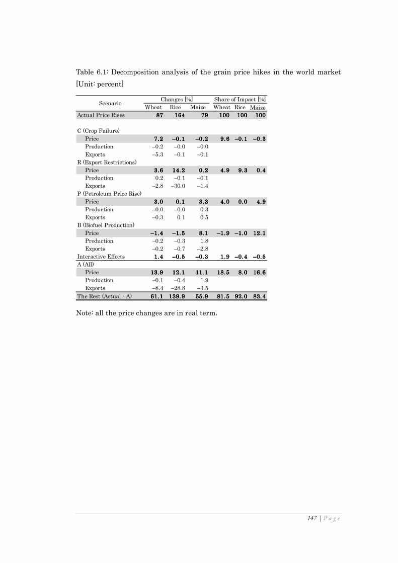
147 | P a g e

Table 6.1: Decomposition analysis of the grain price hikes in the world market

[Unit: percent]

Note: all the price changes are in real term.

Wheat Rice Maize Wheat Rice MaizeActual Price Rises 87878787 164164164164 79797979 100100100100 100100100100 100100100100

C (Crop Failure)

Price 7.27.27.27.2 –0.1–0.1–0.1–0.1 –0.2–0.2–0.2–0.2 9.69.69.69.6 –0.1–0.1–0.1–0.1 –0.3–0.3–0.3–0.3

Production –0.2 –0.0 –0.0

Exports –5.3 –0.1 –0.1

R (Export Restrictions)

Price 3.63.63.63.6 14.214.214.214.2 0.20.20.20.2 4.94.94.94.9 9.39.39.39.3 0.40.40.40.4

Production 0.2 –0.1 –0.1

Exports –2.8 –30.0 –1.4

P (Petroleum Price Rise)

Price 3.03.03.03.0 0.10.10.10.1 3.33.33.33.3 4.04.04.04.0 0.00.00.00.0 4.94.94.94.9

Production –0.0 –0.0 0.3

Exports –0.3 0.1 0.5

B (Biofuel Production)

Price –1.4–1.4–1.4–1.4 –1.5–1.5–1.5–1.5 8.18.18.18.1 –1.9–1.9–1.9–1.9 –1.0–1.0–1.0–1.0 12.112.112.112.1


Exports –0.2 –0.7 –2.8

Interactive Effects 1.41.41.41.4 –0.5–0.5–0.5–0.5 –0.3–0.3–0.3–0.3 1.91.91.91.9 –0.4–0.4–0.4–0.4 –0.5–0.5–0.5–0.5

A (All)

Price 13.913.913.913.9 12.112.112.112.1 11.111.111.111.1 18.518.518.518.5 8.08.08.08.0 16.616.616.616.6


Exports –8.4 –28.8 –3.5

The Rest (Actual - A) 61.161.161.161.1 139.9139.9139.9139.9 55.955.955.955.9 81.581.581.581.5 92.092.092.092.0 83.483.483.483.4

ScenarioChanges [%] Share of Impact [%]

148 | P a g e

Figure 6.1: Changes of grain exports in Scenario A [Unit: percent]

Figure 6.2: World maize export and maize export from the US [Unit: million

tonnes]


149 | P a g e

Figure 6.3: Share of maize export from the US in the world total export [Unit:

percent]


Figure 6.4: Share of maize import by the US to the world total import [Unit:

percent]


6.3 Results: the impacts on the LDCs’ grain markets

The poor wheat harvests in Australia and Ukraine had the greatest

impact of all four factors on increasing the LDC wheat price (Table 6.2). The

wheat price is boosted by export restrictions to almost the same level as by

crop failures. While the international wheat price rises with the petroleum

price hike, the LDC wheat price goes slightly down. This is because the

150 | P a g e

regions rely on import for around 30% of their wheat supply, and their

currencies are appreciated by the oil price hike because some of the LDCs are

oil-rich countries (Figure 6.5).

As in the analysis of the global grain market, the export restrictions

were found to be the most influential of the factors in pushing up the LDC

rice price. The oil price hike also increases the rice price in LDCs, while the

wheat price declines because rice is self-sufficient in the regions, and these

countries do not exploit the advantage of their currencies’ appreciation by the

high oil price, but do suffer from the rising international rice price

transmitted from their rice export. However, the rice price is not greatly

influenced by bad crops and biofuel production.

The LDC maize price is not increased by export restrictions because

only a few countries impose restrictions on their maize export. However, since

the real income in LDCs is restrained by general commodity inflation, the

negative income effect lowers the maize price in Scenario R. The petroleum

price spike causes an increase in income, stimulates the general demand for

commodities, and raises commodity prices, because LDCs do not take

advantage of their currencies’ appreciation as a result of the insulated

domestic market. On the other hand, due to the isolation of the LDCs’ maize

market, the domestic maize markets are only marginally affected by the

higher global maize price caused by biofuel production.

In Scenario A, the prices of wheat, rice and maize rise by around 11%,

19% and 5%. Over half the price rise in rice is accounted for by the four

factors, but these four real-side factors explain the increased prices of wheat

151 | P a g e

and maize by merely 16% and 7%. Hence, for wheat and maize, the

remaining 80%-plus are attributed to other factors. Most of the sensitivity

tests shown in the Appendix find the results robust for wheat and maize. Yet,

when changing the elasticity of substitution for a value-added composite good

from 0.2 to 0.1 or 1.0 for agricultural sectors, the explanatory shares of rice

are very wide-ranging., between 35% and 88%. Considering that the grain

price spikes last for one or two-years, which is short for labour mobility

across sectors, the parameter could be smaller than the 0.2 applied for the

original calculations. Also, it should be noted that comparing the results

between Tables 6.2 and A6.10, the impact shares of rice for Scenario R and P

increase by 47% and 30% respectively, which suggests that the effect of the

export restrictions is more likely to be under-estimated by the changed

elasticity than the effect of the high oil price.1

The oil price hike during the period from 2004 to 2008 raised the

prices of rice and maize by 7.4% and 5.9%, but did not change the price of

wheat very much. The prices of rice and maize are affected more in the LDCs’

markets than in the world’s markets. In Nganou et al. (2009) and Parr and

Wodon (2008), increases of 25% and 34% in the oil price push the maize

price,up by 9% and 6% respectively. Both studies employ linear models, so if

the results of the two papers are applied the price rises in maize are 45% and

22% compared to 126% used in our analysis. These estimates are much

higher than the ones estimated in this thesis. This is primarily because we

1 The estimates are calculated as (47.8−32.7)/32.7 and (31.0−24.7)/24.7.

152 | P a g e

use a non-linear model, which is more flexible in adjusting to the shocks.

It is difficult to explain why an oil price hike and biofuel affect grain

prices because Yang et al (2008) do not reveal the detailed model specification

and how to put shocks into the model. One possibility is that the article

considers biofuel production in China as a shock – the sectors exist in our

model as well, but the production level is not changed as the country does not

have a large share of the world biofuel production, and what is more the

three crops are self-sufficient in China. Another possibility is that their model

assumes farm-land conversion, which affects the impacts of biofuel

production on the prices of wheat and rice. Taking into account the facts that

in China nearly 80% of ethanol production is from maize (APEC, 2008) and

there was relatively little conversion of cultivated land from wheat or rice to

maize during the relevant period (although more farm-land was given to

maize), the results are difficult to be justified by the assumption (Figure 6.6).

Table 6.2: Decomposition analysis of grain price hikes in LDCs

Note: all the price changes are in real term.

Wheat Rice Maize Wheat Rice MaizeActual Price Rises 66.0 30.0 63.0 100.0 100.0 100.0

Impact of;C (Crop Failure) 5.8 -0.1 -0.1 8.8 -0.3 -0.2R (Export Restrictions) 5.0 9.8 -1.1 7.5 32.7 -1.7P (Petroleum Price Rise) -1.4 7.4 5.9 -2.1 24.7 9.3B (Biofuel Production) -0.2 -0.3 0.2 -0.4 -1.1 0.3Interactive Effects 1.5 2.0 -0.3 2.2 6.6 -0.5A (All) 10.7 18.8 4.6 16.2 62.5 7.3The Rest (Actual Price Rises - A) 55.3 11.3 58.4 83.8 37.5 92.7

ScenarioChange in Price [%] Share of Impact [%]

153 | P a g e

Figure 6.5: Self-sufficiency rate of grains in LDCs (production/consumption)

[Unit: percent]


Figure 6.6: Area harvested of grains in China [Unit: hectare]


6.4 Policy Discussions

Lifting export restrictions would have stabilised grain prices,

especially the rice price, in the global market and LDCs. As the domestic

grain price rose through exports even in major exporting countries such as

154 | P a g e

Australia, it might have been reasonable for Russia, a major exporter of

grains, to impose export taxes on grains. Furthermore, the export restrictions

of major exporting nations like India might have been followed by speculators,

who accelerate the price hike. Hence, removing the restrictions would have

been beneficial in preventing the grain price hikes. Meanwhile, export

restrictions limit farmers’ ability to sell their products at higher prices. If it is

a large exporting country like Thailand, the damage from restrictions will be

much greater than the benefit of curbing domestic price rises. As mentioned

in Section 4.1, the number of net sellers of agricultural products is key to the

question of whether poverty is increased by the high price of crops.

Combining this with our simulation results shows that poverty would have

been aggravated if the share of net sellers of rice in the total population had

clearly exceeded that of net buyers in the country. In other words, poor

countries having many net buyers of grains could have benefited from

imposing export restrictions. This is a trade-off between protecting

opportunities for farmers to make more profit by selling grains at higher

prices and safeguarding consumers by suppressing domestic price increases.

Therefore, each country has different optimal export tax rates for grains in

order to maximise the welfare of households when there are grain price hikes

in the global markets.

Biofuel production raises the maize price in the global market but

not in LDCs, and the oil price hike raises the price of crops (except wheat) in

LDCs to some extent. These findings mean that manufacturing biofuel from

non-food feedstock, as proposed by the G8, would contribute to curbing the

155 | P a g e

international maize price. Even if the oil price does spike, the maize price is

less likely to be affected if biofuel is manufactured with non-food material.

Nonetheless, net maize-exporting countries like Cambodia (which exported

50% of its production in 2008) would miss opportunities to make greater

profits with higher maize prices. Yet, many LDCs would not have seriously

suffered from biofuel production in 2008 because of the isolation of their

domestic maize markets – contrary to the popular notion that food prices in

poor nations were increased by biofuel. While the petroleum price increase

makes greater profits for LDCs and their currencies appreciate as some are

rich in oil, the general commodity price rise would have reduced the income of

workers who are not involved in the oil industries, even considering the

spillover effects of greater income as a result of the much increased oil price.

Buffer stocks of grains are versatile in absorbing shocks. If the grain

reserve rate is maintained at high level, it will be less likely to trigger food

speculation even if demand-supply shocks lead to events such as export bans.

Many countries reduced their stock rates to save cost with “just-in-time”

management, but the ratio of world stock to usage should be drawn back to

the previous level of 26% if speculative activities account for much of the

residual of the impacts of our simulations. A negative side of keeping the rate

high is the expensive managing cost that includes labour, land rent,

depreciation of capital stocks etc. Furthermore, although low-income

countries suffer from food price hikes more than rich countries, it is more

difficult for poor nations to hold sufficient grain stocks. However, this

problem might be overcome by the levels of international grain stocks stated

156 | P a g e

in the 2008 G8 meeting (Maeda and Kano, 2008).

Speculation is not examined in this study, but some papers stress it

as a convincing underlying factor (Wei, 2008; Piesse and Thirtle, 2009;, Cooke

and Robles, 2009). If much of the unexplainable portion of our simulation is

accounted for by speculative activities, regulating them would have weakened

the price spikes of grains. Cissokho et al. (2011) propose to impose a

transaction tax on all financial investments in food commodities. Yet, we

should not overlook the fact that farmers are hedging risks on futures

markets. So, whilst the regulations of food speculation protect consumers, the

commodity futures markets contribute to risk management of producers.

6.5 Conclusion

Through Chapters 4 to 6, we attempt to identify the underlying

factors behind the grain price rises in 2008 and analyse the transmitted

impacts on LDCs’ economies. In Chapter 4, the background is introduced, and

the potential factors of the world and LDCs’ grain markets are discussed with

literature reviews. Chapter 5 conducts a discussion on the models used in

earlier studies, and describes the model structure, dataset, and scenarios.

Chapter 6 shows the simulation results of the two types of research,

and derives policy implications based on the calculation outcomes. We find

that the crop failures, export restrictions and biofuel are the greatest

contributory factors among the four for the international price of wheat, rice

and maize. Nevertheless, the price increases in 2008 are not fully explained

by the four factors, and around 80% of the price hikes is still unexplained.

157 | P a g e

Regarding the prices of wheat and rice, the poor harvest shocks and export

restrictions are most critical among the four factors, but biofuel production

does not increase the maize price as much as in popular notion. This is

because only a little amount of maize is exported and imported, and therefore

the international price movement is not transmitted to the LDCs economies

to a large degree. The price hikes of wheat and maize in LDCs are not

sufficiently accounted for by all the four factors. For example, the analysis of

the world price rises finds explanations for about 60% of the rice price

increase. However, the robustness analyses demonstrate a certain

unreliability of the elasticity of substitution for a value-added composite

which implies that the simulated rice price hikes by the export restrictions

can be underestimated with the value of 0.2 for agricultural sectors. However,

the period of the price spikes is only one or two years, which cannot be long

enough for labour forces to move across sectors responding to wage while part

of unskilled labour could change industries even for such a short span.

A limitation of the analyses is that the residual of the price hikes

could not be anatomised while we evaluated the impacts of the primary real-

side factors on food prices. In particular, financial-side factors such as

speculation and the US dollar devaluation are left in the remainder if we

follow the outcomes from past research although other real-side factors not

examined in this analysis might also have affected the grain prices.

158 | P a g e

Appendix: Sensitivity Analyses

Decomposition analysis of the world grain price hikes

In this section we conduct the robustness tests for the main

conclusions of the decomposition analysis by changing elasticity values: the

Armington elasticity, the elasticity for value added composite, the elasticity of

food composite for household, and the elasticity of substitution between

energy goods in both production and household consumption.2

Many of the results support our primary conclusions, but the

elasticity of substitution among factors greatly influences the decomposition

outcome. First, the shares of impact of Scenario A assuming the elasticity

between 0.1 and 1.0 have wide ranges (Tables A6.3 and A6.4). If 0.1 is

assumed, the impact of Scenario A is 37% while it is only 4% when assuming

1.0. Additionally, if 1.0 is assumed, the effect of biofuel is negative and

obviously not the largest among the four. Relatively, rice is less affected by

the parameter change. This is because the primal factors for wheat and maize

price are poor harvest and biofuel production, respectively, both of which are

directly related to the factor substitutability while the largest determinant

for rice is export restrictions. Therefore, the results for rice are found to be

more robust than those of wheat and maize.

2 The elasticity values are indicated in Table 5.4.

159 | P a g e

Table A6.1: Decomposition analysis (the Armington elasticity = 20 for

agricultural sectors)

Table A6.2: Decomposition analysis (the Armington elasticity = −50% for


Table A6.3: Decomposition analysis (elasticity of substitution for value added =

0.1)


Impact of;C (Crop Failure) 5.9 -0.1 -0.1 7.8 -0.1 -0.2R (Export Restrictions) 3.0 13.3 0.7 4.0 8.7 1.1P (Petroleum Price Rise) 2.6 0.3 3.0 3.4 0.2 4.5B (Biofuel Production) -1.3 -1.4 4.8 -1.8 -0.9 7.2Interactive Effects 1.9 -0.4 -0.1 2.6 -0.3 -0.1A (All) 12.0 11.8 8.4 16.0 7.8 12.5The Rest (Actual Price Rises - A) 63.0 140.2 58.6 84.0 92.2 87.5



Impact of;C (Crop Failure) 8.4 -0.1 -0.2 11.2 -0.1 -0.3R (Export Restrictions) 4.3 14.5 0.1 5.7 9.6 0.1P (Petroleum Price Rise) 3.3 -0.1 3.4 4.4 0.0 5.1B (Biofuel Production) -1.5 -1.5 8.0 -2.0 -1.0 11.9Interactive Effects 1.5 -0.6 -0.5 2.0 -0.4 -0.8A (All) 16.0 12.3 10.7 21.3 8.1 16.0The Rest (Actual Price Rises - A) 59.0 139.7 56.3 78.7 91.9 84.0



Impact of;C (Crop Failure) 12.1 -0.2 -0.4 16.2 -0.1 -0.6R (Export Restrictions) 5.4 19.8 -0.2 7.2 13.0 -0.3P (Petroleum Price Rise) 3.0 0.5 4.2 4.0 0.3 6.3B (Biofuel Production) -1.8 -1.7 22.2 -2.4 -1.1 33.1Interactive Effects 4.5 -0.7 -0.8 6.0 -0.5 -1.3A (All) 23.2 17.7 25.0 31.0 11.6 37.3The Rest (Actual Price Rises - A) 51.8 134.3 42.0 69.0 88.4 62.7


160 | P a g e


1.0)

Table A6.5: Decomposition analysis (elasticity of substitution for food composite =

1.0)

Table A6.6: Decomposition analysis (elasticity of substitution for energy goods =

+45%)


Impact of;C (Crop Failure) 3.4 0.0 0.0 4.5 0.0 -0.1R (Export Restrictions) 1.8 8.0 0.4 2.5 5.3 0.6P (Petroleum Price Rise) 3.1 -0.9 2.7 4.2 -0.6 4.1B (Biofuel Production) -1.0 -1.0 -0.6 -1.3 -0.7 -0.9Interactive Effects 0.3 -0.5 -0.1 0.4 -0.3 -0.2A (All) 7.7 5.5 2.4 10.3 3.6 3.5The Rest (Actual Price Rises - A) 67.3 146.5 64.6 89.7 96.4 96.5



Impact of;C (Crop Failure) 5.1 0.0 0.0 6.8 0.0 -0.1R (Export Restrictions) 2.8 8.6 0.4 3.7 5.6 0.6P (Petroleum Price Rise) 2.9 0.2 3.0 3.8 0.1 4.5B (Biofuel Production) -1.3 -1.2 6.3 -1.8 -0.8 9.4Interactive Effects 0.8 -0.4 -0.3 1.0 -0.3 -0.4A (All) 10.2 7.2 9.4 13.6 4.7 14.0The Rest (Actual Price Rises - A) 64.8 144.8 57.6 86.4 95.3 86.0



Impact of;C (Crop Failure) 7.2 -0.1 -0.2 9.6 -0.1 -0.3R (Export Restrictions) 3.6 14.2 0.2 4.9 9.3 0.4P (Petroleum Price Rise) 2.4 -0.6 2.5 3.1 -0.4 3.8B (Biofuel Production) -1.4 -1.5 8.1 -1.9 -1.0 12.1Interactive Effects 1.1 -0.9 -0.6 1.5 -0.6 -0.9A (All) 13.0 11.1 10.1 17.3 7.3 15.1The Rest (Actual Price Rises - A) 62.0 140.9 56.9 82.7 92.7 84.9


161 | P a g e


−45%)

Decomposition analysis of the price spikes in LDCs

With varying the elasticity of substitution, the robustness of the

outcome is checked below. The key findings are that wheat price is pushed up

by the poor harvest and export restrictions while it is pulled down by oil price

rise; the rice price is explained more than half by Scenario A; and biofuel

production does not greatly affect maize price in LDCs.

Crop failure and export restrictions contribute to wheat price. On the

other hand, the petroleum price hike reduces it in all the tests. As stated in

Section 6.3, the elasticity of substitution among factors is a key parameter

that varies the results to a great extent, and less than 50% of the rice price

spike is accounted for by all the factors when assuming the elasticity to be

1.0; however, this is not plausible in the study since the period is not long

enough for labour mobility. Also, assuming the food composite elasticity for

household consumption to be 1.0, the explanatory power of the rice price is

lower than 50%. However, the literature review shown in the Appendix of

Chapter 3 shows that 1.0 is too large for grains. Biofuel production does not

significantly influence the maize price in the original analysis, but if the


Impact of;C (Crop Failure) 7.2 -0.1 -0.2 9.6 -0.1 -0.3R (Export Restrictions) 3.6 14.2 0.2 4.9 9.3 0.4P (Petroleum Price Rise) 3.9 1.0 4.3 5.2 0.7 6.4B (Biofuel Production) -1.4 -1.5 8.1 -1.9 -1.0 12.1Interactive Effects 1.9 -0.1 0.1 2.5 0.0 0.1A (All) 15.2 13.6 12.5 20.3 8.9 18.7The Rest (Actual Price Rises - A) 59.8 138.4 54.5 79.7 91.1 81.3


162 | P a g e

elasticity of the Armington function is assumed to be 20 for agricultural

sectors, the impact is 3%, which is slightly higher than the original

decomposition analysis.

Table A6.8: Decomposition analysis (the Armington elasticity = 20 for


Table A6.9: Decomposition analysis (the Armington elasticity = −50% for


TableA6.10: Decomposition analysis (elasticity of substitution for value added =

0.1)










163 | P a g e


1.0)

Table A6.12: Decomposition analysis (elasticity of substitution for food composite

= 1.0)


+45%)


Impact of;C (Crop Failure) 2.6 0.0 0.0 4.0 -0.1 0.0R (Export Restrictions) 3.2 5.5 -0.2 4.8 18.2 -0.3P (Petroleum Price Rise) -0.9 4.5 2.0 -1.4 15.1 3.1B (Biofuel Production) 0.0 -0.1 0.0 0.0 -0.4 0.0Interactive Effects 0.5 0.6 0.0 0.8 1.9 0.0A (All) 5.4 10.4 1.8 8.2 34.6 2.8The Rest (Actual Price Rises - A) 60.6 19.6 61.2 91.8 65.4 97.2



Impact of;C (Crop Failure) 4.2 0.0 0.0 6.4 0.0 0.0R (Export Restrictions) 4.4 4.1 0.2 6.7 13.8 0.2P (Petroleum Price Rise) -0.9 5.1 4.7 -1.4 16.9 7.4B (Biofuel Production) -0.2 -0.2 0.0 -0.3 -0.5 0.0Interactive Effects 1.1 0.5 0.1 1.7 1.6 0.1A (All) 8.6 9.5 4.9 13.0 31.7 7.8The Rest (Actual Price Rises - A) 57.4 20.5 58.1 87.0 68.3 92.2





164 | P a g e


−45%)




165 | P a g e

7 Conclusion

7.1 Introduction

The thesis has evaluated the risk posed to secure food supply by a

number of factors, and examined them through three empirical studies. This

chapter summarises each chapter. It then describes the methodological

contribution of the thesis and sets out the policy implications which can be

derived from the analysis. Finally, the chapter sets out the limitations of the

analyses.

Chapter 2 showed the methodology used in the thesis. In the first

part, we outlined the composition of a simple single-country and global SAM

with the GTAP database. Next, the equations of a single-country CGE model

were represented, and then it was extended to a world scale. In addition, the

model was delineated as it was transformed for Chapter 3 including the

Monte Carlo method. On the basis of the model for Chapter 3, the model

modifications for Chapters 4, 5, and 6 were also explained.

Chapter 3 addressed Japan’s rice import liberalisation issue. While

free trade is said to enhance the efficiency of resource allocation, the deeper

interdependency of food supply is regarded as a threatening factor for the

importing side. Most of the literature concluded that lowering trade barriers

improves the economic welfare of the importing country with the focus only

on the deterministic impacts, but, hence, do not answer how risky the rice

trade liberalisation is. Developing a stochastic CGE model, we assessed the

risk of the rice trade liberalisation. It was found that trade liberalisation is

166 | P a g e

highly unlikely to endanger Japan’s economy by rice productivity shocks in

the world. However, household welfare in Japan is considerably hampered by

the export bans on rice by the top four rice exporters to Japan. Given that

Japan has experienced only a soybean export embargo by the U.S since World

War II, the benefit from liberalisation will exceed the damage suffered from it.

Further, the emergency rice reserve kept by the government is too large to be

cost effective.

In Chapter 4, we introduced the background of the world food crisis

in 2008 to clarify the objectives of the two studies: the identification of the

driving forces behind the 2008 world grain price rises; and establishing the

factors in the local grain markets in LDCs. The background includes the food

price increases in the international market, food riots in poor countries, the

responses of governments, existing literature concerning price transmission

between world and local markets in developing countries, and the influences

of high agricultural prices on poverty. Then, nine primal potential factors

behind the grain price rises were outlined. These were: the demand growth

in China and India, decline of grain productivity, extreme weather pattern,

oil price hike, emergence of biofuel, export restrictions, devaluation of the US

dollar, food speculation and the low level of world grain stocks. These were

discussed with data and reference to past literature. Finally, the studies

which estimate the effects of a factor(s) on developing economies were

reviewed.

Chapter 5 showed the methodology applied to the two analyses.

Firstly, we critically reviewed the models that quantify the impacts of the

167 | P a g e

possible price drivers. Secondly, the model structure was briefly described.

Next, the regional and sectoral aggregations, the method of creating new

sectors (maize, bioethanol, and biodiesel sectors) in the original GTAP

database, elasticity parameters, and price data were outlined. Finally, the

scenario factors were outlined, namely crop failure, export restrictions, oil

price hike, and biofuel production, and the scenarios were indicated.

Chapter 6 demonstrated the simulation results of the two analyses,

and discussed policy implications. The principal findings for the drivers of the

world grain price hikes were that the four real-side factors poorly explain the

global price rises while crop failure, export restrictions and biofuel production

are crucial factors for the prices of wheat, rice, and maize, respectively. The

same four shocks also account little for the LDC,price hikes of wheat and

maize but over 50% of the rice price spike is explained by the factors,

especially by export restrictions. Another interesting outcome is that biofuel

productions do not raise the maize price in LDCs as the regions have neither

much export nor import of maize. Based on the results, we derive policy

implications related to export restrictions, biofuel policy, buffer grain stocks

and the regulation of speculative activities.

7.2 Methodological contribution

The methodological contribution of the thesis is the application of the

Monte Carlo method to a CGE model. On the topic of Chapter 3, the

literature inspects the liberalisation policy, measuring only the deterministic

effects of Japan lowering trade barriers on rice, and cannot touch the core

168 | P a g e

question of securing its food supply after the free trade. However, the

application of the method to a CGE model makes it possible to evaluate the

stochastic impacts of productivity shocks on the economy from liberalisation,

and to clarify the true benefits (or losses) from abolishing the import tariff on

rice. In the study of Chapter 3, the distribution of rice productivity shocks is

assumed to follow the independent identically distributed normal distribution,

but as long as the form of distribution is specified, it is possible to assess the

probabilistic effects of other types of variable shocks.

7.3 Policy implications

7.3.1 Trade liberalisation

The closed rice market in Japan does not necessarily enhance the

security of food supply according to our simulations. Firstly, the effects of

productivity shocks from abroad are not significant, and productivity shocks

in Japan are considerably more influential on Japan’s households than those

from the outside of Japan. Therefore, free trade raises the mean of welfare of

Japan, and what is more, the variance of welfare is smaller than without

liberalisation. Although our simulations show that rice export bans by major

four trade partners for Japan certainly reduce household welfare in Japan, it

still exceeds 2000 kcal/day/person, which is defined as the most serious level

by the MAFF. Moreover, our simulation outcomes suggest that if rice export is

banned by the major exporting countries every three or four years, the trade

should not be liberalised, in terms of the economic damage. However, from a

169 | P a g e

historical viewpoint, Japan has experienced only one export embargo from

the US on soybean since after the World War II.

The participation in the Trans-Pacific Partnership (TPP) agreement

has aroused a fierce debate in Japan, which involves agricultural sectors. The

major objections are concerned with stable food supply and unemployment.

The former is the subject examined in Chapter 3. Also many of Japan’s

nationals focus on the self-sufficiency rate of food as a means to guarantee

their food supply, but we demonstrate that self-sufficiency does not

necessarily enhance Japan’s food security. Farmers in Japan are not

competitive against those in the US and Australia who are potential

competitors in the agreement because the size of farm-land per farmer in the

US and Australia is as 49 and 316 times large as that in Japan in 2008. The

government promotes the incorporation of small-scale farmers to increase the

number of large-scale ones for greater competitiveness. Taking into account

that consumption depends not only on price but also quality, Japan’s rice

farmers have an advantage as observed in the experience of liberalising the

Japan’s beef market in 1991. It should not be disregarded but is difficult to

assess the environmental value of the rice farming although we do not

analyse it in the thesis.

7.3.2 Grain reserves

The effectiveness of the rice buffer stocks stored by Japan’s

government is measured in Chapter 3. It is shown that the buffer stocks

alleviate negative productivity shocks and contribute to rice price

170 | P a g e

stabilisation. However, the effects of the reserves on welfare do not surpass

the annual maintenance cost. Therefore, we conclude that the government

keeps too much rice in terms of the cost-effectiveness. The storage cost could

be saved by changing to other less expensive locations like Thailand, and

then it could hold more rice reserves.

Considering that the grain price impacts of shocks tend to be large

when the grain stock level is low, we have shown the sensitivity tests in

Chapter 6. However, these do not indicate large differences in the

decomposition analyses from the original results – contrary to the inference

of existing papers such as Timmer (2008) and Piesse and Thirtle (2009).

Grain stocks also have another role, to discourage non-commercial traders

from speculating on rising prices. Although our simulations do not focus on

speculation as a factor of the 2008 food price inflation, there is a possibility

that the combination of the decreased grain reserves with several other

shocks such as the poor harvest in Australia might have triggered speculative

behaviour as Heady and Fan (2008) argue. In other words, food prices might

not have gone up so much if there had been sufficient amount of grain stocks.

According to the results of our robustness tests, grain stocks do not

significantly influence grain prices, but because we have not examined the

amplified effects between speculation, grain reserve and other factors, the

impacts of low grain stock level could be underestimated.

During the food crisis, food riots happened only in poor nations. This

implies that low-income countries suffered from the price spikes of grains

more than rich countries. Yet, national governments lowered their food stock

171 | P a g e

level to save the maintenance costs, which means that destitute countries

had greater difficulty in holding sufficient grain stocks. Maeda and Kano

(2008) analyse the effectiveness of international rice stock, but this issue

should be investigated more in future research.

7.3.3 Export restriction

The analyses of Chapters 4, 5, and 6 demonstrate that export

restrictions bring some impacts on food prices in both the world markets and

LDCs. This conversely means that the annulment of the restrictions would

have lessened the upward volatility but only to a limited degree. However,

the rice price in the global and LDCs’ markets are affected by export

restrictions because international rice market is thinner than other crops,

and even major rice exporting countries such as India banned their rice

export, which corroborates Heady and Fan (2008).

However, as presented in Chapter 3, the larger the exporter a

country is, the greater the sacrifice it needs with its export restrictions. In

addition, if the number of net sellers of a crop is greater than that of net

buyers, poverty will be raised in the country even if it is not a large exporting

country. So, the balance between securing opportunities for farmers to sell

their agricultural products at higher prices and keeping down domestic prices

for consumers is a dilemma for policy makers when facing international price

hikes.

172 | P a g e

7.3.4 Biofuel policy and energy price

Our simulation results show that the emergence of biofuel raises the

price of maize in the world market by only 8% but marginally affects maize

prices in LDCs and wheat and rice prices in both the markets. Namely, even

if the subsidy for biofuel production was abolished, the price increases in

wheat and rice would not have been greatly reduced in 2008. A proposal by

the G8 to manufacture biofuel from non-food feedstock is effective for curbing

price rises to a certain extent but only for the international maize price.

The oil price hike in 2008 increased the grain prices moderately in

global and LDC markets. Causes of the oil price rise are not our focus, but if

it had been raised mainly by speculation, the Oil Trading Transparency Act

discussed in the United States Senate to strengthen the regulation on oil

speculation will work for weakening the oil price fluctuations, but will have a

limited impact on grain prices. Since the oil price hike stimulates biofuel

demand as a substitute, manufacturing biofuel from non-food materials will

further diminish the impact of an oil price increase on food prices.

Meanwhile, the suppression of maize price rises implies that maize

producers may fail to exploit the advantage of selling their maize at more

expensive prices. Some LDCs are net exporters of maize, but as indicated in

our studies, since the maize market in LDCs is rather isolated from other

regions, the price is not seriously affected.

LDCs include several oil-producing countries. The oil price spike

appreciates the LDCs’ currencies, which makes the domestic wheat price

cheaper because around 30% of wheat consumption is dependent on imports

173 | P a g e

while the prices of rice and maize increase as a consequence of not having

much international trade in the products. Nevertheless, workers from outside

the oil industry in LDCs would not have been blessed with the petroleum

price increase, but rather will have seen their real income cut by commodity

inflation.

The US Congress allowed a subsidy for ethanol production to expire

at the end of 2011 (Lever, 2012). In addition to that, bioethanol produced from

maize is not very competitive to oil without a subsidy (Kawashima, 2009).

These facts suggest that bioethanol production in the US will be substantially

discouraged from 2012.

7.3.5 Regulation of speculation

Although we do not analyse the effects of speculation in this thesis,

some papers regard it as a principal factor for the food price hikes in 2008

(Cooke and Robles, 2009;, Wei, 2008; Piesse and Thirtle, 2009). If this is true,

restraining speculation on food markets will be effective in reducing the price

volatility while the futures market functions as a means of risk-hedging for

farmers.

As a matter of fact, the EU tries to levy a tax called “Tobin tax” on

financial transactions to dis-incentivise short-term capital flows (Pop, 2012).

Yet, a major problem is that if there is a region that will not agree with and

will not introduce the tax, it can be a loophole for speculation. Especially

regions that have attracted financial institutions by favourable tax rates so-

called offshore tax havens will not be likely to ratify the agreement. Although

174 | P a g e

it is difficult to impose the financial transaction tax over the whole world,

over 600 agreements on tax transparency and information exchange have

been made since April 2009 (G20-G8 France 2011, 2011).

The Bank of Thailand legislated regulations on the foreign exchange

market in 2006 to control short-term capital flows by requiring investors to

deposit 30% of the investment money into the Bank of Thailand, which was

returned to them if the funds have remained within the country for one year

(Tongurai, 2008). In 1991, Chile put capital controls into effect, which were

found to be significantly effective on capital inflows (Gregorio et al.,

2000).Thus, even if speculation had been an influential factor in the 2008

food crisis, there are still some obstacles to overcome in enforcing the

restrictions, and the issue should be studied.

7.4 Limitations of research

The reservations of the studies of this thesis need to be acknowledged.

First, political aspects are not considered in the analyses. Chapter 3 discusses

the rice trade liberalisation by Japan’s government, which is a politically

sensitive issue since the rice farmers in Japan hold an influential number of

votes, and the government, more specifically the MAFF, has persistently

agitated to protect domestic farming. The chapter has demonstrated the

potential benefit (or risk) from liberalising the rice imports, but it does not

suggest the possibility of the implementation of the policy. For the

implementation of the policy, the political system needs to be discussed with

the result of Chapter 3.

175 | P a g e

Secondly, the trustworthiness of CGE outputs has to be examined.

Kehoe et al. (1995), for instance, confirm that a CGE model perform well in

forecasting the changes in relative prices and resource allocation in the 1986

Spanish fiscal reform, comparing with historical record. Thus, some other

articles affirm the usefulness of CGE models to some extent under some

conditions in the area of free trade, energy, agricultural commodity prices and

so on (Hertel et al., 2007; Beckman and Hertel, 2010; Valenzuela et al., 2007.).

Conversely, Kehoe (2003) argues that a few most prominent static general

equilibrium models extremely underestimate the effects of the North

American Free Trade Agreement (NAFTA), and Hertel et al. (2004) also point

out that the GTAP-AGR model holds the incapability of reproducing wheat

market price volatility. In this thesis, the robustness of the primary

conclusions has been fully checked with sensitivity analyses but publications

concerning this subject are very rare, especially given the recent increase in

CGE model usage.

176 | P a g e

Bibliography

Abbott, P. C., Christopher, H., and Wallace, E. T., 2009. What’s Driving Food

Prices?: March 2009 update. Farm Foundation Issue Report.

Abbott, P. C., Christopher, H., and Wallace, E. T., 2008. What’s Driving Food

Prices? Farm Foundation Issue Report.

Aksoy, M. A., and Isik-Dikmelik, A., 2008. Are Low Food Prices Pro-Poor?: Net

Food Buyers and Sellers in Low-Income Countries. Policy Research

Working Paper 4642, The World Bank.

Aloisi, S., 2011. France, FAO see food crisis risk as prices soar. 4 February 2011,

Reuters. http://uk.reuters.com/article/2011/02/04/uk-food-crisis-

idUKTRE7132NZ20110204

Anderson, K., Martin, W., van der Mensbrugghe, D., 2006. Market and welfare

implications of Doha reform scenarios, in: Anderson, K., Martin, W.

(Eds.), Agricultural Trade Reform and the Doha Development Agenda.

The World Bank, Washington, DC, pp. 333–399.

Asian-Pacific Economic Cooperation (APEC), 2008. China biofuels activities.

http://www.biofuels.apec.org/me_china.html.

Armington, P. S., 1969. A theory of demand for products distinguished by place of

production. International Monetary Fund Staff Pap. 16(1), 159–178.

Arndt, C., Benfica, R., Maximiano, N., Nucifora, A. M. D., and Thurlow, T., 2008.

Higher Fuel and Food Prices: Impacts and Responses for Mozambique.

Agricultural Economics 39, 497-511.

Baffes, J., 1997. Explaining stationary variable with non-stationary regressors.

Applied Economic Letters (4), 69-75.

Barrett, C. B., and Dorosh, P. A., 1996. Farmers’ Welfare and Changing Food

Prices: Nonparametric Evidence from Rice in Madagascar. American

177 | P a g e

Journal of Agricultural Economics 78, 656-669.

Bchir, M., Decreux, H. Y., Guérin, J. and Jean, S., 2002. MIRAGE, A computable

general equilibrium model for trade policy analysis, December CEPII

working paper, No 2002–17.

Beckman, J., Hertel, T. W., and Tyner, W., 2011. Validating Energy-oriented CGE

Models. Energy Economics Article in press.

Burniaux, J., and Truong, T. P., 2002. GTAP-E: An energy-environmental version

of the GTAP model. GTAP Technical Paper No. 16.

Charlebois, P., 2008. The Impact on World Price of Cereals and Oilseeds of Export

Restriction Policies. Agriculture and Agri-Food Canada, Ottawa, Ontario.

Chern, W. S., 2001. Assessment of demand-side factors affecting global food

security. in: Chern, W. S., Carter, C. A., Shei, S. (Eds.), Food Security in

Asia. Edward Elgar, Cheltenham, pp. 83–118.

Chern, W. S., Ishibashi, K., Taniguchi, K., Tokoyama Y., 2002. Analysis of food

Consumption behavior by Japanese households. ESA Working Paper No.

02-06, The Food and Agriculture Organization.

Chino, J., 2000. Kome jukyu moderu-no kozo-to seisan-chosei-no yukue [Demand-

supply model and perspectives of set-aside policy in Japanese rice

economy]. in: Morishima, N. (Ed.), Kokkyo-sochi-to Nihn-nogyo [Trade

Policy and Japanese Agriculture]. Norin-tokei-kyokai, Tokyo, pp. 234–

252 (in Japanese).

Cissokho, M., Lines, T., Nissanke, M., and Smith, A., 2011. Food security, finance

and international trade; how to protect developing countries from

volatile global markets. Veblen Institute for Economic Reforms,

September.

Cooke, B., and R. Robles, 2009. Recent Food Prices Movements: A Time Series

178 | P a g e

Analysis. IFPRI Discussion Paper No. 00942, International Food Policy

Research Institute, Washington, DC.

Cramer, G. L., Hansen, J. M., Wailes, E. J., 1999. Impact of rice tariffication on

Japan and the world rice market. Am. J. Agric. Econ. 81(5), 1149–1156.

Cramer, G. L., Wailes, E. J., Shui, S., 1993. Impacts of liberalizing trade in the

world rice market. Am. J. Agric. Econ. 75(1), 219–226.

Christiaensen, L., and Demery, L., 2007. Down to earth: agriculture and poverty

reduction in Africa. The World Bank.

Cudjoe, G., Breisinger, C., and Diao, X., 2010. Local Impacts of a Global Crisis:

Food Price Transmission, Consumer Welfare, and Poverty in Ghana.

Food Policy 35, 294-302.

Dervis, K., Melo, J. de, and Robinson, S., 1982. General Equilibrium Models for

Development Policy, Cambridge University Press.

Devarajan, S., Lewis, J. D., Robinson, S., 1990. Policy lessons from trade-focused,

two-sector models. J. Policy Modeling 12(4), 625–657.

Dessus, S, Herrera, S., and Hoyos de R, 2008. The impact of food inflation on

urban poverty and its monetary cost: some back-of-the-envelope

calculations. World Bank Policy Research Working Paper 4666.

Francois, J. F. and Roland-Holst, D. W., 1997. Scale economies and imperfect

Competition. in Francois, J. F. and Reinert, K. A. (eds.) Applied methods for

trade policy analysis: a handbook, New York: Cambridge University

Press, Chap. 11, pp. 331–363.

F.O. Licht, 2010. World ethanol and biofuels report. Vol. 9 (08).

G8 Information Centre, 2008. G8 Summits, Hokkaido Official Documents, G8

Leaders Statements on Global Food Security.

G20-G8 France 2011, 2011. Address by the president of the French Republic,

179 | P a g e

Press conference to present the presidency of the G20 and G8. Monday,

24 January 2011. http://www.g20-g8.com/g8-g20/g8/english/for-the-

press/news-releases/press-conference-by-nicolas-sarkozy-monday-

24.933.html.

Gilbert, C., 1989. The impact of exchange rate changes and developing country

debt on commodity prices. Economic Journal (99), 773-784.

Gregorio, J. D., Edwards, S., and Valdes, R. O., 2000. Controls on capital inflows:

do they work? Journal of Development Economics Vol. 63, 59−83.

Harberger, A. C., 1962. The Incidence of the Corporation Tax. Journal of Political

Economy 70, 215-240.

Harris, R. L., Robinson, S., 2001. Economy-wide effects of El Niño/Southern

Oscillation (ENSO) in Mexico and the role of improved forecasting and

technological change. TMD Discussion Paper No. 83, International Food

Policy Research Institute, Washington, DC.

Hasebe, T., 1996. Kome-no hinshitsu-betsu-juyo-to kakaku-hendo [Rice demand

by quality and price fluctuation]. in: Kuroyanagi, T., Kada, R. (Eds.),

Kome-jiyuka-no keiryo-bunseki [Quantitative Analysis on the Rice

Liberalization in Japan]. Taimeido, Tokyo, pp. 13–30 (in Japanese).

Hayami, Y., 2000. Food security: fallacy or reality? in: Chern, S. W., Carter, C. A.,

Shei, S. (Eds.), Food Security in Asia. Edward Elgar, Cheltenham, pp.

11–17.

Heady, D., and Fan, S., 2008. Anatomy of a crisis: the causes and consequences of

surging food prices. IFPRI Discussion Paper 00831.

Hertel, T. W., Hummels, D., Ivanic, M., and Keeney, R., 2007. How Confident Can

We Be of CGE-based Assessments of Free Trade Agreements? Economic

Modelling vol. 24, issue 4, pages 611-635.

180 | P a g e

Hertel, T. W., Keeney, R., and Valenzuela, 2004. Global analysis of agricultural

trade liberalization: assessing model validity. Selected paper prepared

for presentation at the American Agricultural Economics Association

Annual Meeting, Denver, Colorado, July 1-4, 2004.

Hertel, T. W. (Ed.), 1997. Global Trade Analysis. Cambridge University Press,

Cambridge.

Hosoe, N., 2004. Crop failure, price regulation, and emergency imports of Japan’s

rice sector in 1993. Appl. Econ. 36(10), 1051–1056.

Hosoe, N., Gasawa, K., and Hashimoto, H., 2010. Textbook of Computable

General Equilibrium Modeling: Programming and Simulations. Palgrave

Macmillan.

IMF (International Monetary Fund), 2009. IMF Primary Commodity Prices.

Website, http://www.imf.org/external/np/res/commod/index.asp.

International Crop Reserve Research Workshop, 2001. Dai-nikai Kokusai

Bichiku-koso Kenkyukai-iin Yokyu Shiryo [Materials for the Second

Meeting of the International Crop Reserve Research Workshop]. Food

Agency, Ministry of Agriculture, Forestry, and Fishery, Government of

Japan, Tokyo, June 5 (in Japanese).

IRRI, 2008. The rice crisis: what needs to be done? IRRI’s 9-point action plan

http://beta.irri.org/solutions/images/irri/the_rice_crisis_summary.pdf.

Ivanic, M., and Martin, W., 2008. Implications of higher global food prices for

poverty in low-income countries. Agricultural Economics 39, 405-416.

Jayne, T. S., Yamano, T., Nyoro, J., and Awuor, T., 2001. Do Famers Really

Benefit from High Food Prices?: Balancing Rural Interests in Kenya’s

Maize Pricing and Marketing Policy. Tegemeo Working Paper 2B,

Egerton University.

181 | P a g e

Johansen, L., 1960. Multi-sectoral study of growth. Amsterdam, North-Holland.

Kako, T., Gemma, M., Ito, S., 1997. Implications of the minimum access rice

import on supply and demand balance of rice in Japan. Agric. Econ.

16(3): 193–204.

Kawashima, H., 2009. Do not agitate food crisis [shokuryokiki wo aotte ha

ikenai]. Bungei Shunju.

Kehoe, T. J., Polo, C., and Sancho, F., 1995. An evaluation of the performance of

an applied general equilibrium model of the Spanish economy. Economic

Theory vol. 6, pp. 115-141.

Kobayashi, H., 1988. Nihon-no kome-jukyu [Demand and supply of rice in Japan].

in: Oga, K. (Ed.), Kome-no Kokusai-jukyu-to yunyu-jiyuka-mondai

[International Trade of Rice and its Trade Liberalization]. Norin-tokei-

kyokai, Tokyo, pp. 31–73 (in Japanese).

Krugman, P., 1980. Scale economies, product differentiation, and the pattern of

trade. American Economic Review, American Economic Association, vol.

70(5), pages 950-59.

Kusakari, H., 1991. Kome-no hinshitsu-betsu-juyo-to yunyu-jiyuka [Demand for

rice by quality and trade liberalization]. in: Kome-seisaku-kenkyukai

(Ed.), Kome-yunyu-jiyuka-no eikyo-bunseki [Impacts of Rice Import

Liberalization]. Fumin-kyokai, Tokyo, pp. 146–174 (in Japanese).

Lever, R., 2012. US looks ahead after ethanol subsidy expires. 14 January 2012,

AFP, http://www.google.com/hostednews/afp/article/ALeqM5jAkrI-

Apr7LvZ7QPUQz39oe5Jr4w?docId=CNG.2413163943498a313d9d0bab90

35d953.3e1.

Madon, C., 2010. Wheat and corn stockpiles falls as Russian droughts worsens.

12, August, 2010, Daily Finance.

182 | P a g e

http://www.bloggingstocks.com/2010/08/12/wheat-and-corn-stockpiles-

fall-as-russian-drought-worsens/

Maeda, K., Kano, H., 2008. Kokusai-kome-bichiku-ni-yoru shokuryo-anzen-

hosho-to shijo-anteika––kukan-kinko-moderu-ni-yoru keiryo-bunseki

[Food security and market stabilization through international rice

reserve stock: A spatial equilibrium analysis]. Nogyo-keizai-kenkyu 79

(4) [J. Rural Econ.], 199–216 (in Japanese).

MAFF (Ministry of Agriculture, Forestry, and Fisheries), 2008. Report on foreign

food demand and supply in 2008.(in Japanese) [kaigai shokuryo jukyu

repoto 2008].

MAFF (Ministry of Agriculture, Forestry, and Fisheries), Japan, 2006. Fusokuji-

no Shokuryo-anzen-hosho Manyuaru [Food Security Manual for

Contingency Situations]. Tokyo, April (in Japanese).

MAFF (Ministry of Agriculture, Forestry, and Fisheries), Japan, 2001. Dai-nikai

Shokuryo Anzen-hosho Manyuaru Sho-iinkai Giji-roku [Minutes of the

Second Meeting of the Subcommittee for the Food Security Manual].

Tokyo, September 26, (in Japanese).

Martin, W. and Winters, L. A. (eds.), 1996. The Uruguay Round and the

Developing Countries. New York: Cambridge University Press.

McDonald, S., and Thierfelder, K., 2004. Deriving a global social accounting

matrix from GTAP versions 5 and 6 data. GTAP Technical Paper No. 22.

Mensbrugghe, D. van der, 2005. LINKAGE technical reference document version

6.

http://siteresources.worldbank.org/INTPROSPECTS/Resources/334934-

1100792545130/LinkageTechNote.pdf

Metropolis, N., and Ulam, S. M., 1949. The Monte Carlo method. Journal of the

183 | P a g e

American Statistical Association Vol. 44, No. 247.

Meyers, W. H., and Meyer, S., 2008. Causes & implications of the food price surge.

FAPRI-MU Report #12-08, December.

Mitchell, D., 2008. A Note on Rising Food Prices. Policy Research Working

Paper 4682, the World Bank, Washington, DC.

Mitra-Kahn, B. H., 2008. Debunking the Myths of Computable General

Equilibrium Models. SCEPA Working Paper 2008-1.

Miyatake, O., and Nakayama, T., 1960. The Monte Carlo method. (in Japanese)

Nikkan Kogyo Shinbunsha.

Murphy, S., 2008. The Global Food Crisis: Creating an Opportunity for Fairer

and More Sustainable Food and Agriculture System Worldwide. Ecofair

Trade Dialogue Discussion Papers No. 11.

Naylor, R., and Falcon, W., 2010. Food security in an era of economic volatility.

Population and Development Review Vol. 36 (4), pp. 693-723.

Nganou, J. P., Parra, J. C, and Wodon, Q, 2009. Oil price shocks, poverty, and

gender: a social accounting matrix analysis for Kenya. Munich Personal

RePEc Archive (MPRA) Paper No. 28471.

Otsuka, K., 1984. Kome-no juyo-kyokyu-kansu-no suitei [Estimation of rice

demand and supply functions]. Keizai-to keizaigaku 55 [J. the Faculty of

Economics, Tokyo Metropolitan University]: 15–26 (in Japanese).

Parikh, A., 1979. Forecasts of input-output tables using the RAS method. Review

of Economics and Statistics, 61 (3), pp. 477-481.

Parra, J. C., and Wodon, Q, 2008. Comparing the impact of food and energy price

shocks on consumers: a social accounting matrix analysis for Ghana.

World Bank Policy Research Working Paper 4741.

Piesse, J., Thirtle, C., 2009. Three bubbles and a panic: An explanatory review of

184 | P a g e

recent food commodity price events. Food Policy 34 119–129.

Pop, V., 2012. Monti and Merkel: financial tax must cover whole EU. 12 January

2012 euobserver.com, http://euobserver.com/19/114847.

Ravallion, M. and Lokshin, M., 2004. Gainers and losers from trade reform in

Morocco. Middle East and North Africa Working Paper Series No. 37,

The World Bank.

Reuters, 2008. The movement of export restrictions of rice and buffer stock [kome

no yushutsu kisei to zaiko hojuu no ugoki] (in Japanese).

http://jp.reuters.com/article/worldNews/idJPJAPAN-

31611520080501?pageNumber=4&virtualBrandChannel=0, 1st of May,

2008.

Rice Stable Supply Support Organization, Japan, 2007. Seifu-bichiku-mai-

no hanbai-kakaku-no-suii [Sales prices of government rice stocks for

emergencies (October of 2007)], December 25 (in Japanese).

(http://www.komenet.jp/komedata/kakaku/documents/2007/10/4-

10_071225.xls, accessed on September 15, 2010.)

Rosegrant M. W., 2008. Biofuels and Grain Prices: Impacts and Policy Responses.

International Food Policy Research Institute, Washington, DC, May 7.

Rosegrant M. W., Ringler C., Msangi S., Sulser T. B., Zhu T., and Cline S. A.,

2008. International model for policy analysis of agricultural commodities

and trade (IMPACT): model description. International Food Policy

Research Institute website http://www.ifpri.org/book-

751/ourwork/program/impact-model.

Rowley, E., 2011. G20 Paris: Nicolas Sarkozy calls for action against inflation’s

‘great threat’. The Telegraph, 19, February, 2011.

http://www.telegraph.co.uk/finance/g20-summit/8334770/G20-Paris-

185 | P a g e

Nicolas-Sarkozy-calls-for-action-against-inflations-great-threat.html

Sawada, M., 1985. Shokuryo-juyo-to hinshitsu [Food demand and quality]. in:

Sakiura, S. (Ed.), Keizai-hatten-to nogyo-kaihatsu [Economic

Development and Agricultural Development]. Norin-tokei-kyokai, Tokyo,

pp. 70–89 (in Japanese).

Sawada, Y., 1984. Komerui-juyo-no keiryo-bunseki [Quantitative analysis of rice

demand]. in: Sakiura, S. (Ed.), Kome-no keizai-bunseki [Economic

Analysis of Rice]. Norin-tokei-kyokai, Tokyo, pp. 139–153 (in Japanese).

Scarf, H. E., 1973. The Computation of Economic Equilibria, Yale University

Press.

Science Council of Japan, 2001. Chikyu-kankyo Ningen-seikatsu-ni-kakawaru

Nogyo-oyobi-shinrin-no Tamenteki-na-kino-no Hyoka-ni-tsuite (Toshin)

[Report on the Multi-functionality of Agriculture and Forest for Global

Environment and Human Life], Tokyo, November (in Japanese).

Sharma, R., 2011. Food Export Restrictions: Review of the 2007-2010 Experience

and Considerations for Disciplining Restrictive Measures. FAO

Commodity And Trade Policy Research Working Paper No. 32.

Shoven, J. B., and Whalley, J., 1992. Applying General Equilibrium, Cambridge

University Press.

Smil, V., 2000. Feeding the World. Massachusetts Institute of Technology.

Taheripour, F., Birur, D. K., Hertel, T. W., and Tyner, W. E., 2008. Introducing

Liquid Biofuels into GTAP Data Base. GTAP Research Memorandum No.

11.

Tanaka, T., and Hosoe, N., 2011a. What Drove the Crop Price Hikes in the Food

Crisis? GRIPS Discussion Papers 11-16.

Tanaka, T., and Hosoe, N., 2011b. Does Agricultural Trade Liberalization

186 | P a g e

Increase Risks of Supply-side Uncertainty?: Effects of Productivity

Shocks and Export Restrictions on Welfare and Food Supply in Japan.

Food Policy 36(3), 368–377.

Tongrai, J., 2008. Baht appreciation and the Bank of Thailand’s foreign exchange

intervention: experience in 2001-March 2008.

Trostle, R., 2008. Global Agricultural Supply and Demand: Factors Contributing

to the Recent Increase in Food Commodity Prices. USDA, A Report from

the Economic Research Service WRS-0801.

USDA (United States Department of Agriculture), 2008. China, Peoples Republic

of, Agricultural Situation, 2008 China Tightens Control on Grain and

Flour Exports. GAIN Report No. CH8001, January 14.

Valenzuela, E. and Hertel, T. W., 2007. Assessing Global Computable General

Equilibrium Model Validity Using Agricultural Price Volatility. American

Journal of Agricultural Economics, vol. 89, issue 2, pages 383-397

Von Braun, J., 2008. Rising Food Prices: What Should Be Done? IFPRI Policy

Brief April 2008.

Von Braun, J., Ahmed, A., Asenso-Okyere, K., Fan, S., Gulati, A., Hoddinott, J.,

Pandya-Lorch, R., Rosegrant, M. W., Ruel, M, Torero, M., Van Rheenen,

T., and Von Grebmer, K., 2008. High Food Prices: The What, Who, and

How of Proposed Policy Actions. Policy Brief May 2008. IFPRI.

Wailes, E. J., 2005. Rice: global trade, protectionist policies, and the impact of

trade liberalization, in: Aksoy, M. A., Beghin, J. C. (Eds.), Global

Agricultural Trade and Developing Countries. The World Bank,

Washington, DC, pp. 177–193.

Wei Ruan, 2008. World grain price hikes. (in Japanese) [Sekai teki na kokumotsu

kakaku no koutou], Nihon Keizai Shinbun, 23, July, 2008.

187 | P a g e

Whalley, J., 1982. An Evaluation of the Recent Tokyo Round Trade Agreement

Using General Equilibrium Computation Methods, Journal of Policy

Modelling 4, 341-361.

Wodon, Q., and Zaman, H., 2008. Rising food prices in sub-saharan Africa:

poverty impact and Policy responses. World Bank Policy Research

Working Paper 4738.

Wodon, Q., Tsimpo, C., Backiny-Yetna, P., Joseph, G., Adoho, F., and Coulombe,

H., 2008. Potential impact of higher food prices on poverty: summary

estimates for a dozen west and central African countries. World Bank

Policy Research Working Paper, 4745.

World Bank, 2011. Food Price Hike Drives 44 Million People into Poverty. No:

2011/333/PREM.

World Bank, 2008a. Competitive Agriculture or State Control: Ukraine's

Response to the Global Food Crisis. Europe and Central Asia Region,

Sustainable Development Unit, May, Washington DC.

World Bank, 2008b. Group of Eight, Meeting of Finance of Ministers, Osaka,

Addressing the Food Crisis: The Need for Rapid and Coordinated Action.

Wright, B. D., 2011. The Economics of Price Volatility. Applied Economic

Perspectives and Policy 33 (1), 32–58.

Yang, J., Qiu, H., Huang, J., and Rozelle, S., 2008. Fighting Global Food Price

Rises in the Developing World: The Response of China and its Effect on

Domestic and World Markets. Agricultural Economics 39 (1), 453–464.

Download (1496Kb) - SOAS Research Online - SOAS, University of

Documents

Transcript of Download (1496Kb) - SOAS Research Online - SOAS, University of