Doubly Convolutional Neural Networks

Shuangfei ZhaiBinghamton UniversityVestal, NY 13902, USA

szhai2@binghamton.edu

Yu ChengIBM T.J. Watson Research Center

Yorktown Heights, NY 10598, USAchengyu@us.ibm.com

Weining LuTsinghua UniversityBeijing 10084, China

luwn14@mails.tsinghua.edu.cn

Zhongfei (Mark) ZhangBinghamton UniversityVestal, NY 13902, USA

zhongfei@cs.binghamton.edu

Abstract

Building large models with parameter sharing accounts for most of the success ofdeep convolutional neural networks (CNNs). In this paper, we propose doubly con-volutional neural networks (DCNNs), which significantly improve the performanceof CNNs by further exploring this idea. In stead of allocating a set of convolutionalfilters that are independently learned, a DCNN maintains groups of filters wherefilters within each group are translated versions of each other. Practically, a DCNNcan be easily implemented by a two-step convolution procedure, which is supportedby most modern deep learning libraries. We perform extensive experiments onthree image classification benchmarks: CIFAR-10, CIFAR-100 and ImageNet, andshow that DCNNs consistently outperform other competing architectures. We havealso verified that replacing a convolutional layer with a doubly convolutional layerat any depth of a CNN can improve its performance. Moreover, various designchoices of DCNNs are demonstrated, which shows that DCNN can serve the dualpurpose of building more accurate models and/or reducing the memory footprintwithout sacrificing the accuracy.

1 Introduction

In recent years, convolutional neural networks (CNNs) have achieved great success to solve manyproblems in machine learning and computer vision. CNNs are extremely parameter efficient dueto exploring the translation invariant property of images, which is the key to training very deepmodels without severe overfitting. While considerable progresses have been achieved by aggressivelyexploring deeper architectures [1, 2, 3, 4] or novel regularization techniques [5, 6] with the standard"convolution + pooling" recipe, we contribute from a different view by providing an alternative to thedefault convolution module, which can lead to models with even better generalization abilities and/orparameter efficiency.

Our intuition originates from observing well trained CNNs where many of the learned filters are theslightly translated versions of each other. To quantify this in a more formal fashion, we define thek-translation correlation between two convolutional filters within a same layer Wi,Wj as:

ρk(Wi,Wj) = maxx,y∈{−k,...,k},(x,y) 6=(0,0)

<Wi, T (Wj , x, y) >f

‖Wi‖2‖Wj‖2, (1)

where T (·, x, y) denotes the translation of the first operand by (x, y) along its spatial dimensions,with proper zero padding at borders to maintain the shape; < ·, · >f denotes the flattened inner

30th Conference on Neural Information Processing Systems (NIPS 2016), Barcelona, Spain.

Figure 1: Visualization of the 11× 11 sized first layer filters learned by AlexNet [1]. Each columnshows a filter in the first row along with its three most 3-translation-correlated filters. Only the first32 filters are shown for brevity.

Figure 2: Illustration of the averaged maximum 1-translation correlation, together with the standarddeviation, of each convolutional layer for AlexNet [1] (left), and the 19-layer VGGNet [2] (right),respectively. For comparison, for each convolutional layer in each network, we generate a filter setwith the same shape from the standard Gaussian distribution (the blue bars). For both networks, allthe convolutional layers have averaged maximum 1-translation correlations that are significantlylarger than their random counterparts.

product, where the two operands are flattened into column vectors before taking the standard innerproduct; ‖ · ‖2 denotes the `2 norm of its flattened operand. In other words, the k-translationcorrelation between a pair of filters indicates the maximum correlation achieved by translating onefilter up to k steps along any spatial dimension. As a concrete example, Figure 1 demonstratesthe 3-translation correlation of the first layer filters learned by the AlexNet [1], with the weightsobtained from the Caffe model zoo [7]. In each column, we show a filter in the first row and its threemost 3-translation-correlated filters (that is, filters with the highest 3-translation correlations) in thesecond to fourth row. Only the first 32 filters are shown for brevity. It is interesting to see for mostfilters, there exist several filters that are roughly its translated versions.

In addition to the convenient visualization of the first layers, we further study this property athigher layers and/or in deeper models. To this end, we define the averaged maximum k-translationcorrelation of a layer W as ρ̄k(W) = 1

N

∑Ni=1 maxN

j=1,j 6=i ρk(Wi,Wj), where N is the numberof filters. Intuitively, the ρ̄k of a convolutional layer characterizes the average level of translationcorrelation among the filters within it. We then load the weights of all the convolutional layers ofAlexNet as well as the 19-layer VGGNet [2] from the Caffe model zoo, and report the averagedmaximum 1-translation correlation of each layer in Figure 2. In each graph, the height of the redbars indicates the ρ̄1 calculated with the weights of the corresponding layer. As a comparison,for each layer we have also generated a filter bank with the same shape but filled with standardGaussian samples, whose ρ̄1 are shown as the blue bars. We clearly see that all the layers in bothmodels demonstrate averaged maximum translation correlations that are significantly higher thantheir random counterparts. In addition, it appears that lower convolutional layers generally havehigher translation correlations, although this does not strictly hold (e.g., conv3_4 in VGGNet).

Motivated by the evidence shown above, we propose the doubly convolutional layer (with the doubleconvolution operation), which can be plugged in place of a convolutional layer in CNNs, yieldingthe doubly convolutional neural networks (DCNNs). The idea of double convolution is to learngroups filters where filters within each group are translated versions of each other. To achieve this, adoubly convolutional layer allocates a set of meta filters which has filter sizes that are larger than theeffective filter size. Effective filters can be then extracted from each meta filter, which corresponds toconvolving the meta filters with an identity kernel. All the extracted filters are then concatenated, andconvolved with the input. Optionally, one can also choose to pool along activations produced by filtersfrom the same meta filter, in a similar spirit to the maxout networks [8]. We also show that doubleconvolution can be easily implemented with available deep learning libraries by utilizing the efficient

2

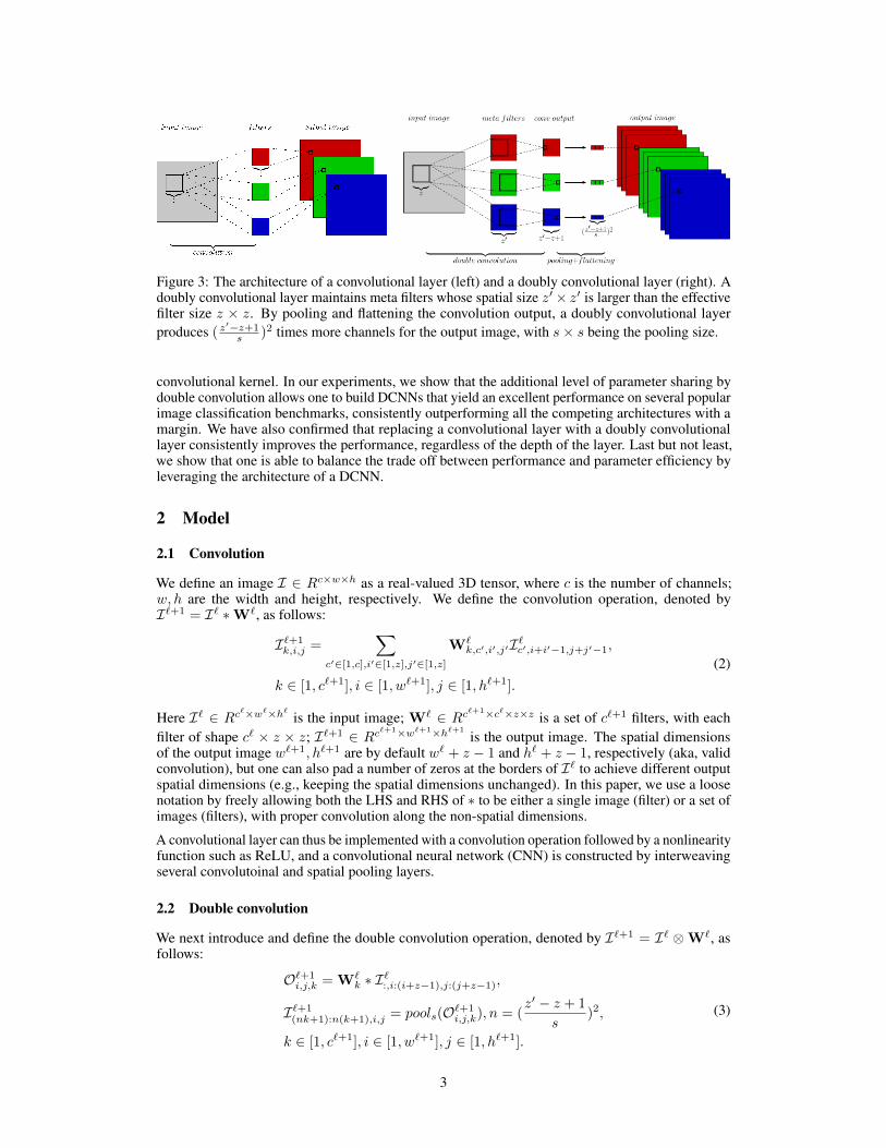
Figure 3: The architecture of a convolutional layer (left) and a doubly convolutional layer (right). Adoubly convolutional layer maintains meta filters whose spatial size z′× z′ is larger than the effectivefilter size z × z. By pooling and flattening the convolution output, a doubly convolutional layerproduces ( z′−z+1

s )2 times more channels for the output image, with s× s being the pooling size.

convolutional kernel. In our experiments, we show that the additional level of parameter sharing bydouble convolution allows one to build DCNNs that yield an excellent performance on several popularimage classification benchmarks, consistently outperforming all the competing architectures with amargin. We have also confirmed that replacing a convolutional layer with a doubly convolutionallayer consistently improves the performance, regardless of the depth of the layer. Last but not least,we show that one is able to balance the trade off between performance and parameter efficiency byleveraging the architecture of a DCNN.

2 Model

2.1 Convolution

We define an image I ∈ Rc×w×h as a real-valued 3D tensor, where c is the number of channels;w, h are the width and height, respectively. We define the convolution operation, denoted byI`+1 = I` ∗W`, as follows:

I`+1k,i,j =

∑c′∈[1,c],i′∈[1,z],j′∈[1,z]

W`k,c′,i′,j′I`c′,i+i′−1,j+j′−1,

k ∈ [1, c`+1], i ∈ [1, w`+1], j ∈ [1, h`+1].

(2)

Here I` ∈ Rc`×w`×h`

is the input image; W` ∈ Rc`+1×c`×z×z is a set of c`+1 filters, with eachfilter of shape c` × z × z; I`+1 ∈ Rc`+1×w`+1×h`+1

is the output image. The spatial dimensionsof the output image w`+1, h`+1 are by default w` + z − 1 and h` + z − 1, respectively (aka, validconvolution), but one can also pad a number of zeros at the borders of I` to achieve different outputspatial dimensions (e.g., keeping the spatial dimensions unchanged). In this paper, we use a loosenotation by freely allowing both the LHS and RHS of ∗ to be either a single image (filter) or a set ofimages (filters), with proper convolution along the non-spatial dimensions.

A convolutional layer can thus be implemented with a convolution operation followed by a nonlinearityfunction such as ReLU, and a convolutional neural network (CNN) is constructed by interweavingseveral convolutoinal and spatial pooling layers.

2.2 Double convolution

We next introduce and define the double convolution operation, denoted by I`+1 = I` ⊗W`, asfollows:

O`+1i,j,k = W`

k ∗ I`:,i:(i+z−1),j:(j+z−1),

I`+1(nk+1):n(k+1),i,j = pools(O`+1

i,j,k), n = (z′ − z + 1

s)2,

k ∈ [1, c`+1], i ∈ [1, w`+1], j ∈ [1, h`+1].

(3)

3

Here I` ∈ Rc`×w`×h`

and I`+1 ∈ Rnc`+1×w`+1×h`+1

are the input and output image, respectively.W` ∈ Rc`+1×c`×z′×z′

are a set of c`+1 meta filters, with filter size z′ × z′, z′ > z; O`+1i,j,k ∈

R(z′−z+1)×(z′−z+1) is the intermediate output of double convolution; pools(·) defines a spatialpooling function with pooling size s × s (and optionally reshaping the output to a column vector,inferred from the context); ∗ is the convolution operator defined previously in Equation 2.

In words, a double convolution applies a set of c`+1 meta filters with spatial dimensions z′ × z′,which are larger than the effective filter size z × z. Image patches of size z × z at each location(i, j) of the input image, denoted by I`:,i:(i+z−1),j:(j+z−1), are then convolved with each meta filter,resulting an output of size z′ − z + 1× z′ − z + 1, for each (i, j). A spatial pooling of size s× s isthen applied along this resulting output map, whose output is flattened into a column vector. Thisproduces an output feature map with nc`+1 channels. The above procedure can be viewed as a twostep convolution, where image patches are first convolved with meta filters, and the meta filters thenslide across and convolve with the image, hence the name double convolution.

A doubly convolutional layer is by analogy defined as a double convolution followed by a nonlinearity;and substituting the convolutional layers in a CNN with doubly convolutional layers yields a doublyconvolutional neural network (DCNN). In Figure 3 we have illustrated the difference between aconvolutional layer and a doubly convolutional layer. It is possible to vary the combination of z, z′, sfor each doubly convolutional layer of a DCNN to yield different variants, among which three extremecases are:

(1) CNN: Setting z′ = z recovers the standard CNN; hence, DCNN is a generalization of CNN.

(2) ConcatDCNN: Setting s = 1 produces a DCNN variant that is maximally parameter efficient.This corresponds to extracting all sub-regions of size z × z from a z′ × z′ sized meta filter, whichare then stacked to form a set of (z′ − z + 1)2 filters with size z × z. With the same amount ofparameters, this produces (z′−z+1)2z2

(z′)2 times more channels for a single layer.

(3) MaxoutDCNN: Setting s = z′− z+ 1, i.e., applying global pooling onO`+1, produces a DCNNvariant where the output image channel size is equal to the number of the meta filters. Interestingly,this yields a parameter efficient implementation of the maxout network [8]. To be concrete, themaxout units in a maxout network are equivalent to pooling along the channel (feature) dimension,where each channel corresponds to a distinct filter. MaxoutDCNN, on the other hand, pools alongchannels which are produced by the filters that are translated versions of each other. Besides theobvious advantage of reducing the number of parameters required, this also acts as an effectiveregularizer, which is verified later in the experiments at Section 4.

Implementing a double convolution is also readily supported by most main stream GPU-compatibledeep learning libraries (e.g., Theano which is used in our experiments), which we have summarizedin Algorithm 1. In particular, we are able to perform double convolution by two steps of convolution,corresponding to line 4 and line 6, together with proper reshaping and pooling operations. The firstconvolution extracts overlapping patches of size z× z from the meta filters, which are then convolvedwith the input image. Although it is possible to further reduce the time complexity by designing aspecialized double convolution module, we find that Algorithm 1 scales well to deep DCNNs, andlarge datasets such as ImageNet.

3 Related work

The spirit of DCNNs is to further push the idea of parameter sharing of the convolutional layers,which is shared by several recent efforts. [9] explores the rotation symmetry of certain classes ofimages, and hence proposes to rotate each filter (or alternatively, the input) by a multiplication of90◦ which produces four times filters with the same amount of parameters for a single layer. [10]observes that filters learned by ReLU CNNs often contain pairs with opposite phases in the lowerlayers. The authors accordingly propose the concatenated ReLU where the linear activations areconcatenated with their negations and then passed to ReLU, which effectively doubles the number offilters. [11] proposes the dilated convolutions, where additional filters with larger sizes are generatedby dilating the base convolutional filters, which is shown to be effective in dense prediction taskssuch as image segmentation. [12] proposes a multi-bias activation scheme where k, k ≤ 1, biasterms are learned for each filter, which produces a k times channel size for the convolution output.

4

Algorithm 1: Implementation of double convolution with convolution.

Input: Input image I` ∈ Rc`×w`×h`

, meta filters W` ∈ Rc`+1×z′×z′ , effective filter sizez × z, pooling size s× s.

Output: Output image I`+1 ∈ Rnc`+1×w`+1×h`+1

, with n = (z′−z+1)2

s2.

1 begin2 I` ← IdentityMatrix (c`z2) ;3 Reorganize I` to shape c`z2 × c` × z × z;4 W̃` ←W` ∗ I` ; /* output shape: c`+1 × c`z2 × (z′ − z + 1)× (z′ − z + 1) */5 Reorganize W̃` to shape c`+1(z′ − z + 1)2 × c` × z × z;6 O`+1 ← I` ∗ W̃` ; /* output shape: c`+1(z′ − z + 1)2 × w`+1 × h`+1 */7 Reorganize O`+1 to shape c`+1w`+1h`+1 × (z′ − z + 1)× (z′ − z + 1) ;8 I`+1 ← pools(O`+1) ; /* output shape: c`+1w`+1h`+1 × z′−z+1

s× z′−z+1

s*/

9 Reorganize I`+1 to shape c`+1( z′−z+1

s)2 × w`+1 × h`+1 ;

Additionally, [13, 14] have investigated the combination of more than one transformations of filters,such as rotation, flipping and distortion. Note that all the aforementioned approaches are orthogonalto DCNNs and can theoretically be combined in a single model. The need of correlated filters inCNNs is also studied in [15], where similar filters are explicitly learned and grouped with a groupsparsity penalty.

While DCNNs are designed with better performance and generalization ability in mind, they arealso closely related to the thread of work on parameter reduction in deep neural networks. Thework of Vikas and Tara [16] addresses the problem of compressing deep networks by applyingstructured transforms. [17] exploits the redundancy in the parametrization of deep architectures byimposing a circulant structure on the projection matrix, while allowing the use of FFT for fastercomputations. [18] attempts to obtain the compression of the fully-connected layers of the AlexNet-type network with the Fastfood method. Novikov et al. [19] use a multi-linear transform (Tensor-Traindecomposition) to attain reduction of the number of parameters in the linear layers of CNNs. Thesework differ from DCNNs as most of their focuses are on the fully connected layers, which oftenaccounts for most of the memory consumption. DCNNs, on the other hand, apply directly to theconvolutional layers, which provides a complementary view to the same problem.

4 Experiments

4.1 Datasets

We conduct several sets of experiments with DCNN on three image classification benchmarks:CIFAR-10, CIFAR-100, and ImageNet. CIFAR-10 and CIFAR-100 both contain 50,000 trainingand 10,000 testing 32× 32 sized RGB images, evenly drawn from 10 and 100 classes, respectively.ImageNet is the dataset used in the ILSVRC-2012 challenge, which consists of about 1.2 millionimages for training and 50,000 images for validation, sampled from 1,000 classes.

4.2 Is DCNN an effective architecture?

4.2.1 Model specifications

In the first set of experiments, we study the effectiveness of DCNN compared with two differentCNN designs. The three types of architectures subject to evaluation are:

(1) CNN: This corresponds to models using the standard convolutional layers. A convolutional layeris denoted as C-<c>-<z>, where c, z are the number of filters and the filter size, respectively.

(2) MaxoutCNN: This corresponds to the maxout convolutional networks [8], which uses the maxoutunit to pool along the channel (feature) dimensions with a stride k. A maxout convolutional layer isdenoted as MC-<c>-<z>-<k>, where c, z, k are the number of filters, the filter size, and the featurepooling stride, respectively.

5

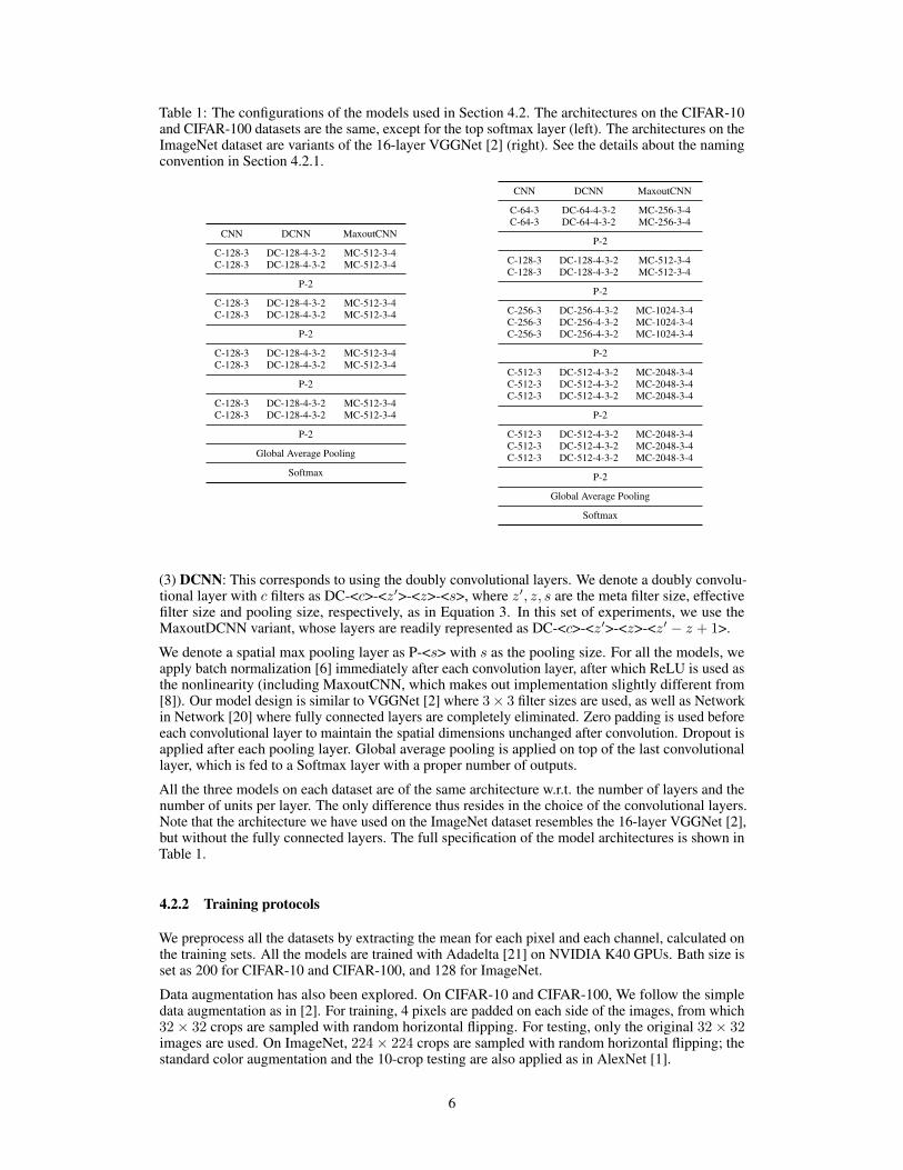
Table 1: The configurations of the models used in Section 4.2. The architectures on the CIFAR-10and CIFAR-100 datasets are the same, except for the top softmax layer (left). The architectures on theImageNet dataset are variants of the 16-layer VGGNet [2] (right). See the details about the namingconvention in Section 4.2.1.

CNN DCNN MaxoutCNN

C-128-3 DC-128-4-3-2 MC-512-3-4C-128-3 DC-128-4-3-2 MC-512-3-4

P-2

C-128-3 DC-128-4-3-2 MC-512-3-4C-128-3 DC-128-4-3-2 MC-512-3-4

P-2

C-128-3 DC-128-4-3-2 MC-512-3-4C-128-3 DC-128-4-3-2 MC-512-3-4

P-2

C-128-3 DC-128-4-3-2 MC-512-3-4C-128-3 DC-128-4-3-2 MC-512-3-4

P-2

Global Average Pooling

Softmax

CNN DCNN MaxoutCNN

C-64-3 DC-64-4-3-2 MC-256-3-4C-64-3 DC-64-4-3-2 MC-256-3-4

P-2

C-128-3 DC-128-4-3-2 MC-512-3-4C-128-3 DC-128-4-3-2 MC-512-3-4

P-2

C-256-3 DC-256-4-3-2 MC-1024-3-4C-256-3 DC-256-4-3-2 MC-1024-3-4C-256-3 DC-256-4-3-2 MC-1024-3-4

P-2

C-512-3 DC-512-4-3-2 MC-2048-3-4C-512-3 DC-512-4-3-2 MC-2048-3-4C-512-3 DC-512-4-3-2 MC-2048-3-4

P-2

C-512-3 DC-512-4-3-2 MC-2048-3-4C-512-3 DC-512-4-3-2 MC-2048-3-4C-512-3 DC-512-4-3-2 MC-2048-3-4

P-2

Global Average Pooling

Softmax

(3) DCNN: This corresponds to using the doubly convolutional layers. We denote a doubly convolu-tional layer with c filters as DC-<c>-<z′>-<z>-<s>, where z′, z, s are the meta filter size, effectivefilter size and pooling size, respectively, as in Equation 3. In this set of experiments, we use theMaxoutDCNN variant, whose layers are readily represented as DC-<c>-<z′>-<z>-<z′ − z + 1>.

We denote a spatial max pooling layer as P-<s> with s as the pooling size. For all the models, weapply batch normalization [6] immediately after each convolution layer, after which ReLU is used asthe nonlinearity (including MaxoutCNN, which makes out implementation slightly different from[8]). Our model design is similar to VGGNet [2] where 3× 3 filter sizes are used, as well as Networkin Network [20] where fully connected layers are completely eliminated. Zero padding is used beforeeach convolutional layer to maintain the spatial dimensions unchanged after convolution. Dropout isapplied after each pooling layer. Global average pooling is applied on top of the last convolutionallayer, which is fed to a Softmax layer with a proper number of outputs.

All the three models on each dataset are of the same architecture w.r.t. the number of layers and thenumber of units per layer. The only difference thus resides in the choice of the convolutional layers.Note that the architecture we have used on the ImageNet dataset resembles the 16-layer VGGNet [2],but without the fully connected layers. The full specification of the model architectures is shown inTable 1.

4.2.2 Training protocols

We preprocess all the datasets by extracting the mean for each pixel and each channel, calculated onthe training sets. All the models are trained with Adadelta [21] on NVIDIA K40 GPUs. Bath size isset as 200 for CIFAR-10 and CIFAR-100, and 128 for ImageNet.

Data augmentation has also been explored. On CIFAR-10 and CIFAR-100, We follow the simpledata augmentation as in [2]. For training, 4 pixels are padded on each side of the images, from which32× 32 crops are sampled with random horizontal flipping. For testing, only the original 32× 32images are used. On ImageNet, 224× 224 crops are sampled with random horizontal flipping; thestandard color augmentation and the 10-crop testing are also applied as in AlexNet [1].

6

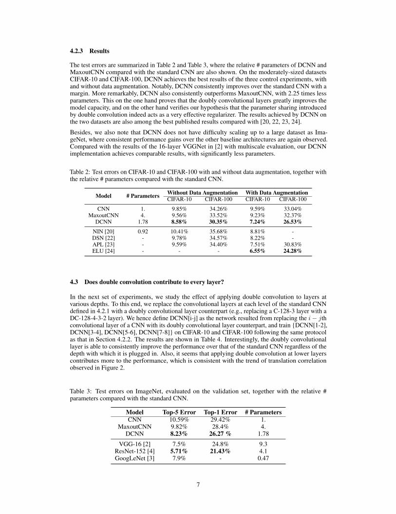
4.2.3 Results

The test errors are summarized in Table 2 and Table 3, where the relative # parameters of DCNN andMaxoutCNN compared with the standard CNN are also shown. On the moderately-sized datasetsCIFAR-10 and CIFAR-100, DCNN achieves the best results of the three control experiments, withand without data augmentation. Notably, DCNN consistently improves over the standard CNN with amargin. More remarkably, DCNN also consistently outperforms MaxoutCNN, with 2.25 times lessparameters. This on the one hand proves that the doubly convolutional layers greatly improves themodel capacity, and on the other hand verifies our hypothesis that the parameter sharing introducedby double convolution indeed acts as a very effective regularizer. The results achieved by DCNN onthe two datasets are also among the best published results compared with [20, 22, 23, 24].

Besides, we also note that DCNN does not have difficulty scaling up to a large dataset as Ima-geNet, where consistent performance gains over the other baseline architectures are again observed.Compared with the results of the 16-layer VGGNet in [2] with multiscale evaluation, our DCNNimplementation achieves comparable results, with significantly less parameters.

Table 2: Test errors on CIFAR-10 and CIFAR-100 with and without data augmentation, together withthe relative # parameters compared with the standard CNN.

Model # Parameters Without Data Augmentation With Data AugmentationCIFAR-10 CIFAR-100 CIFAR-10 CIFAR-100

CNN 1. 9.85% 34.26% 9.59% 33.04%MaxoutCNN 4. 9.56% 33.52% 9.23% 32.37%

DCNN 1.78 8.58% 30.35% 7.24% 26.53%

NIN [20] 0.92 10.41% 35.68% 8.81% -DSN [22] - 9.78% 34.57% 8.22% -APL [23] - 9.59% 34.40% 7.51% 30.83%ELU [24] - - - 6.55% 24.28%

4.3 Does double convolution contribute to every layer?

In the next set of experiments, we study the effect of applying double convolution to layers atvarious depths. To this end, we replace the convolutional layers at each level of the standard CNNdefined in 4.2.1 with a doubly convolutional layer counterpart (e.g., replacing a C-128-3 layer with aDC-128-4-3-2 layer). We hence define DCNN[i-j] as the network resulted from replacing the i− jthconvolutional layer of a CNN with its doubly convolutional layer counterpart, and train {DCNN[1-2],DCNN[3-4], DCNN[5-6], DCNN[7-8]} on CIFAR-10 and CIFAR-100 following the same protocolas that in Section 4.2.2. The results are shown in Table 4. Interestingly, the doubly convolutionallayer is able to consistently improve the performance over that of the standard CNN regardless of thedepth with which it is plugged in. Also, it seems that applying double convolution at lower layerscontributes more to the performance, which is consistent with the trend of translation correlationobserved in Figure 2.

Table 3: Test errors on ImageNet, evaluated on the validation set, together with the relative #parameters compared with the standard CNN.

Model Top-5 Error Top-1 Error # ParametersCNN 10.59% 29.42% 1.

MaxoutCNN 9.82% 28.4% 4.DCNN 8.23% 26.27 % 1.78

VGG-16 [2] 7.5% 24.8% 9.3ResNet-152 [4] 5.71% 21.43% 4.1GoogLeNet [3] 7.9% - 0.47

7

Table 4: Inserting the doubly convolutional layer at different depths of the network.

Model CIFAR-10 CIFAR-100CNN 9.85% 34.26%

DCNN[1-2] 9.12% 32.91%DCNN[3-4] 9.23% 33.27%DCNN[5-6] 9.45% 33.58%DCNN[7-8] 9.57% 33.72%DCNN[1-8] 8.58% 30.35%

4.4 Performance vs. parameter efficiency

In the last set of experiments, we study the behavior of DCNNs under various combinations of itshyper-parameters, z′, z, s. To this end, we train three more DCNNs on CIFAR-10 and CIFAR-100,namely {DCNN-32-6-3-2, DCNN-16-6-3-1, DCNN-4-10-3-1}. Here we have overloaded the notationfor a doubly convolutional layer to denote a DCNN which contains correspondingly shaped doublyconvolutional layers (the DCNN in Table 1 thus corresponds to DCNN-128-4-3-2). In particular,DCNN-32-6-3-2 produces a DCNN with the exact same shape and number of parameters of those ofthe reference CNN; DCNN-16-6-3-1, DCNN-4-10-3-1 are two ConcatDCNN instances from Section2.2, which produce larger sized models with same or less amount of parameters. The results, togetherwith the effective layer size and the relative number of parameters, are listed in Table 5. We see thatall the variants of DCNN consistently outperform the standard CNN, even when fewer parametersare used (DCNN-4-10-3-1). This verifies that DCNN is a flexible framework which allows one toeither maximize the performance with a fixed memory budget, or on the other hand, minimize thememory footprint without sacrificing the accuracy. One can choose the best suitable architecture of aDCNN by balancing the trade off between performance and the memory footprint.

Table 5: Different architecture configurations of DCNNs.

Model CIFAR-10 CIFAR-100 Layer size # Parameters

CNN 9.85% 34.26% 128 1.DCNN-32-6-3-2 9.05% 32.28% 128 1.DCNN-16-6-3-1 9.16% 32.54% 256 1.DCNN-4-10-3-1 9.65% 33.57% 256 0.69

DCNN-128-4-3-2 8.58% 30.35% 128 1.78

5 Conclusion

We have proposed the doubly convolutional neural networks (DCNNs), which utilize a novel doubleconvolution operation to provide an additional level of parameter sharing over CNNs. We show thatDCNNs generalize standard CNNs, and relate to several recent proposals that explore parameterredundancy in CNNs. A DCNN can be easily implemented by modern deep learning librariesby reusing the efficient convolution module. DCNNs can be used to serve the dual purpose of 1)improving the classification accuracy as a regularized version of maxout networks, and 2) beingparameter efficient by flexibly varying their architectures. In the extensive experiments on CIFAR-10,CIFAR-100, and ImageNet datasets, we have shown that DCNNs significantly improves over otherarchitecture counterparts. In addition, we have shown that introducing the doubly convolutionallayer to any layer of a CNN improves its performance. We have also experimented with variousconfigurations of DCNNs, all of which are able to outperform the CNN counterpart with the same orfewer number of parameters.

References[1] Alex Krizhevsky, Ilya Sutskever, and Geoffrey E Hinton. Imagenet classification with deep convolutional

neural networks. In Advances in neural information processing systems, pages 1097–1105, 2012.

8

[2] Karen Simonyan and Andrew Zisserman. Very deep convolutional networks for large-scale image recogni-tion. arXiv preprint arXiv:1409.1556, 2014.

[3] Christian Szegedy, Wei Liu, Yangqing Jia, Pierre Sermanet, Scott Reed, Dragomir Anguelov, DumitruErhan, Vincent Vanhoucke, and Andrew Rabinovich. Going deeper with convolutions. In Proceedings ofthe IEEE Conference on Computer Vision and Pattern Recognition, pages 1–9, 2015.

[4] Kaiming He, Xiangyu Zhang, Shaoqing Ren, and Jian Sun. Deep residual learning for image recognition.arXiv preprint arXiv:1512.03385, 2015.

[5] Nitish Srivastava, Geoffrey Hinton, Alex Krizhevsky, Ilya Sutskever, and Ruslan Salakhutdinov. Dropout:A simple way to prevent neural networks from overfitting. The Journal of Machine Learning Research,15(1):1929–1958, 2014.

[6] Sergey Ioffe and Christian Szegedy. Batch normalization: Accelerating deep network training by reducinginternal covariate shift. arXiv preprint arXiv:1502.03167, 2015.

[7] Yangqing Jia, Evan Shelhamer, Jeff Donahue, Sergey Karayev, Jonathan Long, Ross Girshick, SergioGuadarrama, and Trevor Darrell. Caffe: Convolutional architecture for fast feature embedding. InProceedings of the ACM International Conference on Multimedia, pages 675–678. ACM, 2014.

[8] Ian J Goodfellow, David Warde-Farley, Mehdi Mirza, Aaron Courville, and Yoshua Bengio. Maxoutnetworks. arXiv preprint arXiv:1302.4389, 2013.

[9] Sander Dieleman, Jeffrey De Fauw, and Koray Kavukcuoglu. Exploiting cyclic symmetry in convolutionalneural networks. arXiv preprint arXiv:1602.02660, 2016.

[10] Wenling Shang, Kihyuk Sohn, Diogo Almeida, and Honglak Lee. Understanding and improving con-volutional neural networks via concatenated rectified linear units. arXiv preprint arXiv:1603.05201,2016.

[11] Fisher Yu and Vladlen Koltun. Multi-scale context aggregation by dilated convolutions. arXiv preprintarXiv:1511.07122, 2015.

[12] Hongyang Li, Wanli Ouyang, and Xiaogang Wang. Multi-bias non-linear activation in deep neural networks.arXiv preprint arXiv:1604.00676, 2016.

[13] Robert Gens and Pedro M Domingos. Deep symmetry networks. In Advances in neural informationprocessing systems, pages 2537–2545, 2014.

[14] Taco S Cohen and Max Welling. Group equivariant convolutional networks. arXiv preprintarXiv:1602.07576, 2016.

[15] Koray Kavukcuoglu, Rob Fergus, Yann LeCun, et al. Learning invariant features through topographicfilter maps. In Computer Vision and Pattern Recognition, 2009. CVPR 2009. IEEE Conference on, pages1605–1612. IEEE, 2009.

[16] Vikas Sindhwani, Tara Sainath, and Sanjiv Kumar. Structured transforms for small-footprint deep learning.In C. Cortes, N. D. Lawrence, D. D. Lee, M. Sugiyama, and R. Garnett, editors, Advances in NeuralInformation Processing Systems 28, pages 3088–3096. Curran Associates, Inc., 2015.

[17] Yu Cheng, Felix X. Yu, Rogerio Feris, Sanjiv Kumar, and Shih-Fu Chang. An exploration of parameterredundancy in deep networks with circulant projections. In International Conference on Computer Vision(ICCV), 2015.

[18] Zichao Yang, Marcin Moczulski, Misha Denil, Nando de Freitas, Alex Smola, Le Song, and Ziyu Wang.Deep fried convnets. In International Conference on Computer Vision (ICCV), 2015.

[19] Alexander Novikov, Dmitry Podoprikhin, Anton Osokin, and Dmitry Vetrov. Tensorizing neural networks.In Advances in Neural Information Processing Systems 28 (NIPS). 2015.

[20] Min Lin, Qiang Chen, and Shuicheng Yan. Network in network. arXiv preprint arXiv:1312.4400, 2013.

[21] Matthew D Zeiler. Adadelta: an adaptive learning rate method. arXiv preprint arXiv:1212.5701, 2012.

[22] Chen-Yu Lee, Saining Xie, Patrick Gallagher, Zhengyou Zhang, and Zhuowen Tu. Deeply-supervised nets.arXiv preprint arXiv:1409.5185, 2014.

[23] Forest Agostinelli, Matthew Hoffman, Peter J. Sadowski, and Pierre Baldi. Learning activation functionsto improve deep neural networks. CoRR, abs/1412.6830, 2014.

[24] Djork-Arné Clevert, Thomas Unterthiner, and Sepp Hochreiter. Fast and accurate deep network learningby exponential linear units (elus). arXiv preprint arXiv:1511.07289, 2015.

9