Journal of Petroleum Science and Engineering 78 (2011) 65–77

Contents lists available at ScienceDirect

Journal of Petroleum Science and Engineering

j ourna l homepage: www.e lsev ie r.com/ locate /pet ro l

Double-porosity model for tracer transport in reservoirs having open conductivegeological faults: Determination of the fault orientation

Manuel Coronado ⁎, Jetzabeth Ramírez-Sabag, Oscar Valdiviezo-MijangosInstituto Mexicano del Petróleo, Eje Central Lázaro Cárdenas 152, 07730 México D.F., Mexico

⁎ Corresponding author. Tel.: +52 55 9175 8302.E-mail address: mcoronad@imp.mx (M. Coronado).

0920-4105/$ – see front matter © 2011 Elsevier B.V. Aldoi:10.1016/j.petrol.2011.04.002

a b s t r a c t

a r t i c l e i n f o

Article history:Received 26 February 2010Accepted 6 April 2011Available online xxxx

Keywords:tracerfaulttransportflowmodel

Conductive geological faults in oil reservoirs have a major impact in the efficiency of fluid-flooding andenhanced oil recovery schemes. Inter-well tracer tests are a traditional mean to determine undergroundcommunication channel properties, and therefore have the potential to estimate fault features. In this work ananalytical model is developed to describe inter-well tracer tests in reservoirs with open conductive faults.Specifically, a fault that intersects the flow path between the injection and production wells without reachingthem is treated. In open faults fluid can be exchanged along the fault to external regions. In addition, thepresent model captures two new relevant aspects of the process: (i) the fault region is a fractured media, and(ii) a Danckwert's discharge condition is established at production well. To treat open faults a new source-coupling scheme is designed for linking the three independent path regions in which the system isdiscomposed. The first region comprehends the path from the injector to the fault, the second represents thezone along the fault, and the third one the path from the fault to the production well. The involved coupledadvection–dispersion equations are analytically solved by the Laplace technique and numerically inverted.There are twelve parameters in the model; from them five concern the fault properties. By exploring theireffect on the tracer breakthrough curve it is found that the curve is mainly sensitive to the tracer fault pathlength and the fault fluid velocity. The two factors describing the fracture–matrix coupling become importantonly when the fluid velocity in the fault is relatively low. No relevant sensitivity is found on the faultdispersivity. An outstanding attractive feature of the new model is its capacity to determine the faultorientation, which is not possible by the standard characterization means. The model has been successfullyapplied to data from a real reservoir tracer test performed in Loma Alta Sur Field. Here, the orientation of twofaults have been determined.

l rights reserved.

© 2011 Elsevier B.V. All rights reserved.

1. Introduction

Determining the main underground communication channels ina reservoir is of primary interest in fluid flooding and improvedoil recovery programs. Highly conductive channels are generallyundesired since they dramatically reduce flood sweep efficiency byproviding direct underground flow paths and hence by-passingremaining oil. If the presence and properties of these channels areknown, their effect can be incorporated in the flooding project design;for example, by properly selecting the injection well location or bysealing problematic channels. Geological faults work frequently astransverse flow barriers but they can also work as longitudinal orvertical flow conduits depending on the fault structure. Faultscommonly comprise a low permeability plane core which is flankedat both sides by the so called damage zones. These zones are frequentlyhigh permeable regions with a complex network of small fractures

and veins (Bense and Person, 2006; Caine et al., 1996; Fairley andHinds, 2004). Therefore, reservoir fluids can move straightforwardlyalong conductive faults.

Inter-well tracer tests are traditionally employed in oil reservoirs tocharacterize communication channels and validate reservoir geologicalmodels. In these tests, a tracer is introduced in the formation throughan injection well, and its appearance is observed in the surroundingproduction wells. From the tracer breakthrough curves, fundamentalinformation on the conductive channels and formation characteristicscan be obtained. In order to interpret tracer tests, diverse analysis toolsbecome helpful. In this context, mathematical models for tracer testsstand as a fundamental platform.Many analytical andnumericalmodelshave been developed along the years to describe inter-well tracertransport in underground formations. However, only few analyticalmodels capture a common feature in oil reservoirs, which is that theinjection or production wells in the formation are located outside thefault plane (Coronado and Ramírez-Sabag, 2008; Houseworth, 2004).Therefore, the inter-well tracer route comprehends not only the pathalong the fault itself, but also a path section from the injectionwell to thefault, and another section from the fault to the production well. These

(A)

(B)

Fig. 1. Schematic representation of the fluid flow in the fault for the cases (A) fault-dominated flow and (B) injection-dominated flow.

Fig. 2. Three coupled one-dimensional flow regions.

66 M. Coronado et al. / Journal of Petroleum Science and Engineering 78 (2011) 65–77

two additional path sections have in general non-negligible length,and definitively impact the final tracer breakthrough curve shape. Theworks mentioned above partially take this fact in account. In hisreport, Houseworth (2004) represents the conductive fault by a highlypermeable streak surrounded by lowpermeability rockmatrix. Uniformfluid flow parallel and transversal to the fault is assumed. Tracertransport is determined by considering: advection in the fault, fracture–matrix diffusive exchange, tracer adsorption and radioactive decay.However twomain issues are lacking: longitudinal tracer dispersion andthe presence of the third path section, from the fault to the productionwell. In the work by Coronado and Ramírez-Sabag (2008), a closedfluid system composed by three aligned regionswith different transportproperties, plus an injector and a production well is assumed. Theamount of injectionfluidflowing througheachof the three regions is thesame. Convective flow aswell as longitudinal dispersion was taken intoaccount in the three regions; however the fractured media features ofthe central region were neglected.

In this paper a newmodel to describe tracer transport in reservoirshaving a conductive fault as well as injection and production wellsoutside the fault plane is presented. Three new aspects have beenincorporated with respect to the previous model by Coronado andRamírez-Sabag (2008). (i) The fluid system is not closed, in the sensethat fluid can be exchanged along the fault to the external inter-wellregions. To treat this first issue a new approach based on source-coupled regions has been introduced. (ii) Diffusive coupling betweenthe fracture network and the matrix rock in the damage zones of thecentral path section (fault region) is taken into account by consideringa double-porosity model for this region. (iii) Finally, the Danckwert'sboundary condition at the production well is established (Schwartzet al., 1999). This new formulation enhances the applicabilitypotential of the previous models and allows the determination ofthe fault orientation. This is a completely new feature not possiblewhen using the regular reservoir characterization techniques.

2. Model description

The system under study considers a fluid injection well, aproduction well, and a conductive fault between them, as illustratedin Fig. 1. Two flow situations are analyzed. The first situation is shownin Fig. 1(A) and describes a case when a strong flow along the fault ispresent. The fluid from the injector reaches the fault and it is thenincorporated to the main fault flow and carried by it. The secondsituation is displayed in Fig. 1(B) and corresponds to the case whenflow dynamics in the fault is dominated by the injection flow; hence, adivergent flow in the fault is established: one part of the injected fluidgoes to the left side along the fault and another part to the right side.The first case will be referred as fault-dominated flow and the secondas injection-dominated flow.

In order to model the tracer transport, the system is simplified ascomposed by three independent one-dimensional regions as shown inFig. 2. A constant velocity is assumed in each region. The first regioncomprehends the path from the injection well to the fault. The tracermotion associated to the fluid velocity u1 is described by using the spacevariable x1. There is an injection well located at x1=0 and the fault atx1=L1. The second region corresponds to the fault section, and itsbehavior is described using the space variable x2. A tracer source is set atx2=0, which takes into account the tracer arriving from Region 1. Thissource makes the coupling between both regions, and it represents aninnovation in the new approach. The fluid velocity in the central faultsection is u2, in the left fault section is u2, L, and in the right fault sectionu2,R. The total tracer path length along the fault is L2. The third region isdescribed by the space variable x3, where the fluid moves at velocity u3.The tracer source due to the tracer appearing from Region 2 into Region3 is located at x3=0. The production well is located at x3=L3.

As previouslymentioned, the fluid flow in each region is decoupledfrom the fluid flow in the other two regions; however the tracer

dynamics is coupled through sources. This assumption has beenintroduced in order to facilitate the mathematics while keeping themain tracer transport features. In reality, a relationship between thefluid velocity in the three sections exists since fluid mass is conserved.This condition establishes that the fluid mass flow,q, must beconserved at coupling interfaces. There is however no contradictionwith the decoupled velocity assumption made, since some additionalparameters are involved in the mass conservation requirement. Anexplanation of this issue is as follows. The continuity of the fluid massflow, qi=uiAiϕiρ, sets conditions on the product of velocity ui timeseffective channel cross-section ϕiAi (where Ai and ϕi are macroscopicchannel cross-section and porosity of Region i, and ρ fluid density).Thus, there is no fluid mass conservation failure by pre-establishingthe velocity in each section, since ϕiAi is still unknown.

For x1b0 in Region 1 the velocity is set as −u1, and for x1N0 as u1.This pattern represents a one-dimensional linear divergent injectionflow, as illustrated in Fig. 3(A). In Region 2 the velocity in the centralsection was established as u2, together with u2,R=u2, as displayed in

(A)

(B)

(C)

Fig. 3. Three separated flow systems.

Fig. 4. The standard double-porosity system in Region 2.

67M. Coronado et al. / Journal of Petroleum Science and Engineering 78 (2011) 65–77

Fig. 3(B). In this region a two-dimensional system (x2,z) is taken inorder to consider a fractured porous medium, as will be describedbelow. In the left section u2, L=u2 is set for the fault-dominated flowcase, and u2, L=−u2 for the injection-dominated flow case. In Region3 the velocity is u3.

The mathematical problem consists in determining the tracerconcentration in each region, which is given by C1(x1, t), C2(x2,z, t) andC3(x3, t) respectively. An initial Dirac delta pulse in Region 1 will beassumed. Region 2 will be treated as a fractured porous mediumwhile Region 1 and Region 3 as non-fractured media. Advection andlongitudinal dispersion will be considered in all three regions.

2.1. Region 1

The one-dimensional system for Region 1 corresponds to a classicalproblem. It considers a divergent linear flow around the injection wellat x1=0. The initial condition is

C1 x1; t = 0ð Þ = mA1ϕ1

δ x1ð Þ; ð1Þ

where m is the tracer mass injected and δ(x1) the Dirac delta. Theboundary conditions are

C1 x1→� ∞; tð Þ = 0: ð2Þ

The advection–dispersion equation for this region is

∂C1

∂t + u1 x1ð Þ ∂C1

∂x1−D1

∂2C1

∂x21= 0; ð3Þ

where u1(x1) is u1 for x1≥0 and −u1 for x1b0. The dispersioncoefficient D1 is constant and given by D1=α1|u1|, with α1 thedispersivity of Region 1. The Laplace transform of Eq. (3) yields

sC1 x1; sð Þ + u1 x1ð Þ∂C1 x1; sð Þ∂x1

−D1∂2C1 x1; sð Þ

∂x21=

mA1ϕ1

δ x1ð Þ: ð4Þ

For x1N0 it means

sC1 x1; sð Þ + u1∂C1 x1; sð Þ

∂x1−D1

∂2C1 x1; sð Þ∂x21

= 0; ð5Þ

and for x1b0

sC1 x1; sð Þ−u1∂C1 x1; sð Þ

∂x1−D1

∂2C1 x1; sð Þ∂x21

= 0: ð6Þ

The solution that satisfies C1 x1 = 0−; sð Þ = C1 x1 = 0þ; sð Þ is

C1 x1; sð Þ = B sð Þ exp γ sð Þ jx1 jð Þ; ð7Þ

which is symmetric in x1 with

γ sð Þ = u1

2D11−

ffiffiffiffiffiffiffiffiffiffiffiffiffiffiffiffiffiffiffiffiffiffiffiffiffiffiffiffiffiffi1 + 4sD1 = u

21

q� �b 0: ð8Þ

Tracermass conservation at x1=0 provides a condition to evaluateB(s). This condition can be obtained by integrating Eq. (4) from x1=−ε to x1=ε and then taking the limiting situation ε→0. It yields thecondition

−D1∂C1

∂x1 jx1 =0−

−∂C1

∂x1 jx1 =0þ

" #+ 2u1C1 x1 = 0ð Þ = m

A1ϕ1: ð9Þ

After substituting Eq. (7) it gives

B sð Þ = m= A1ϕ1u1

1 +ffiffiffiffiffiffiffiffiffiffiffiffiffiffiffiffiffiffiffiffiffiffiffiffiffiffiffiffiffiffi1 + 4sD1 = u

21

q : ð10Þ

The tracer mass rate that arrives at point x=L1 at time t is

M∘1 = A1ϕ1J1 x1 = L1; tð Þ; ð11Þ

where J1 is the tracer mass flux, which for any region i is given by

Ji xi; tð Þ = ui xið ÞCi xi; tð Þ−Di∂Ci xi; tð Þ

∂xi: ð12Þ

The quantity M1∘

defines the tracer source in the second region.

2.2. Region 2

Region 2 corresponds to a fractured porous media, and thereforethe well known double-porosity model is employed (Coronado etal., 2007; Maloszewski and Zuber, 1985). The conventional two-dimensional system is introduced, which comprehends the fracturenetwork and a porous matrix, as illustratively shown in Fig. 4. In thefracture network the tracer moves subject to advection, longitudinaldispersion and also diffusion into the surrounding porous matrix. Inthe porous matrix no advection occurs, only tracer diffusion and rocksurface tracer adsorption/desorption reactions are present. The spacevariable along the fracture is designed by x2 and the perpendicularspace variable by z (see Fig. 3(B)). The effective fracture width is2w and the effective matrix block size E. The tracer concentration in

68 M. Coronado et al. / Journal of Petroleum Science and Engineering 78 (2011) 65–77

the fracture network is Cf(x2, t) and in the matrix Cm(x2,z, t). Thecorresponding porosity is ϕf and ϕm respectively. The tracerdispersion coefficient in the fracture network is given by Df and thediffusion coefficient in the matrix porous media by Dm. As previouslymentioned, the fluid velocity in the fracture system is assumedconstant. As shown in Fig. 3(B) this velocity is u2 for x2N0, however,for x2b0 it is−u2 in the injection-dominated case and u2 in the fault-dominated case.

The transport equation for the tracer fracture network populationis given by

∂Cf

∂t + u2 x2ð Þ ∂Cf

∂x2−Df

∂2Cf

∂x22−ϕmDm

b∂Cm

∂z jz=w

= S2 tð Þδ x2ð Þ; ð13Þ

and for the porous matrix population by

∂Cm

∂t −Dm

R∂2Cm

∂z2= 0; ð14Þ

where u2(x) is the step-function described before, and R is a tracerretardation factor due to rock adsorption/desorption. Eqs. (13) and(14) have the standard form (Coronado et al., 2007; Maloszewski andZuber, 1985), except by the source term S2(t). This source term isthe tracer amount arriving from Region 1 per unit of cross-section. TheDirac delta function δ(x2) locates the source at x2=0. The tracersource rate S2 is the term M

∘1 from Eq. (11) divided by channel cross-

section in Region 2. Thus

S2 tð Þ = A1ϕ1

A2ϕ2J1 x1 = L1; tð Þ: ð15Þ

The boundary conditions are the traditional, i.e.

Cf x2→� ∞; tð Þ = 0; ð16Þ

Cm x2; z = w; t N 0ð Þ = Cf x2; tð Þ; ð17Þ

∂Cm

∂z jE =2

= 0; ð18Þ

plus a new initial condition, which states that no tracer is present inRegion 2 at t=0

Cf x2; t = 0ð Þ = 0; ð19Þ

Cm x2; z; t = 0ð Þ = 0: ð20Þ

The Laplace transform of Eqs. (13) and (14) yields

sCf + u2 x2ð Þ∂Cf

∂x2−Df

∂2Cf

∂x22−ϕmDm

b∂Cm

∂z jz=w

= S2 sð Þδ x2ð Þ ð21Þ

sCm−Dm

R∂2Cm

∂z2= 0 ð22Þ

The Laplace transform of the source is evaluated by using Eqs. (15),(12) and (7); it follows

S2 sð Þ = u1A1ϕ1

2A2ϕ21 +

ffiffiffiffiffiffiffiffiffiffiffiffiffiffiffiffiffiffiffiffiffiffiffiffiffiffiffiffiffiffi1 + 4sD1 = u

21

q� �B sð Þexp γL1ð Þ: ð23Þ

The solution of the equation set is found by following the standardprocedure. First, Eq. (22) is solved to find

Cm x2; z; sð Þ = Wþ x2; sð Þexp k zð Þ + W− x2; sð Þexp −k zð Þ; ð24Þ

whereW+ andW− are functions to be determined and k =ffiffiffiffiffiffiffiffiffiffiffiffiffiffiffiffisR=Dm

p.

Further, the multiple fracture condition in Eq. (18) implies

Cm x2; z; sð Þ = Wþ x2; sð Þexp k zð Þ 1 + exp 2k E = 2−zð Þð Þ½ �; ð25Þ

which after setting Eq. (17) yields

Cm x2; z; sð Þ = Cf x2; sð Þexp k z−bð Þ½ � 1 + exp 2k E = 2−zð Þð Þ½ �1 + exp 2k E = 2−wð Þð Þ½ � : ð26Þ

By using this expression the last term in the LHS of Eq. (21) can beevaluated. It is

∂Cm

∂z jz=w

= −βCf tanh k E = 2ð Þw½ �: ð27Þ

Therefore, the equation for Cf x2; sð Þ in Eq. (21) translates into

σ sð ÞCf x2; sð Þ + u2 x2ð Þ∂Cf

∂x2−Df

∂2Cf

∂x22= S2 sð Þδ x2ð Þ; ð28Þ

with σ(s) defined as

σ sð Þ = s +ffiffis

p ϕmDm

w

� � ffiffiffiffiffiffiffiRDm

stanh

ffiffiffiffiffiffiffiffiffiffiffiffiffiffiffiffisR=Dm

pE = 2−wð Þ

h i: ð29Þ

Eq. (28) can be solved in Laplace domain by seeking for solutionsof the form Cf∝exp(γ x2). First the case x2≠0 is taken, where nocontribution from the Dirac delta term appears. Later, the jump inx2=0 is taken into account. The solutions are obtained in terms of thefunctions

ξ� sð Þ = u2

2Df1�

ffiffiffiffiffiffiffiffiffiffiffiffiffiffiffiffiffiffiffiffiffiffiffiffiffiffiffiffiffiffi1 + 4σDf =u

22

q� �; ð30Þ

where ξ−b0 and ξ+N0. They specifically depend on the constantvalue u2(x2b0); therefore, the cases of injection-dominated flow andfault-dominated flow will yield different results.

2.2.1. Injection-dominated flow: u2(x2b0)=−u2:The solution for x2≠0 satisfying the boundary condition in Eq. (16)

and continuity at point x2=0 is

Cf x2; sð Þ = Y sð Þexp −ξ−x2ð Þ x2 b 0

Y sð Þexp ξ−x2ð Þ x2 N 0:

(ð31Þ

The derivative jump condition at x2=0 obtained from Eq. (28)gives

2Y sð Þ u2−Df ξ− sð Þh i

= S2 sð Þ; ð32Þ

which after substitution of ξ− it yields

Y sð Þ = S2 =u2

1 +ffiffiffiffiffiffiffiffiffiffiffiffiffiffiffiffiffiffiffiffiffiffiffiffiffiffiffiffiffiffiffi1 + 4σDf =u

22

q ð33Þ

2.2.2. Fault-dominated flow: u2(x2b0)=u2The solution for x2≠0 satisfying the boundary condition in

Eq. (16) and continuity at x2=0 is

Cf x2; sð Þ = Y sð Þ exp ξþx2� �

x2 b 0

Y sð Þexp ξ−x2ð Þ x2 N 0:

(ð34Þ

69M. Coronado et al. / Journal of Petroleum Science and Engineering 78 (2011) 65–77

The derivative jump condition at x2=0 obtained from Eq. (28)is now

Y sð ÞDf ξþ sð Þ−ξ− sð Þ = S2 sð Þ; ð35Þ

which yields

Y sð Þ = S2 =u2ffiffiffiffiffiffiffiffiffiffiffiffiffiffiffiffiffiffiffiffiffiffiffiffiffiffiffiffiffiffi1 + 4σDf =u

22

q ð36Þ

2.3. Region 3

This third region represents the tracer path from the fault planeto the production well. It corresponds to a non-fractured mediawith similar properties as Region 1. The fluid velocity is constant asillustrated in Fig. 3(C). The boundary conditions to be set on the tracerconcentration are

C3 x3→−∞; tð Þ = 0; ð37Þ

and the Danckwert's discharge condition at the production well, i.e. atx3=L3. This yields a vanishing tracer dispersive flow at the productionwell (Schwartz et al., 1999),

∂C3

∂x3 jx3 =L3

= 0: ð38Þ

which represents that there is no porous media inside the well. Theinitial condition of no tracer present in Region 3 at the initial timereads

C3 x3; t = 0ð Þ = 0: ð39Þ

Further, by following the same ideas as in the previous regiona tracer source is set at x3=0, which takes into account the tracerarriving from Region 2. The tracer transport equation is

∂C3

∂t + u3∂C3

∂x3−D3

∂2C3

∂x23= S3 tð Þδ x3ð Þ; ð40Þ

and the tracer source rate

S3 tð Þ = A2ϕ2FA3ϕ3

J2 x2 = L2; tð Þ: ð41Þ

The tracer flow J2(x2, t)is obtained from Eq. (12) with Ci=Cf(x2, t)and Di=Df. The parameter F is a factor that describes the tracerfraction transferred from Region 2 into Region 3, hence 0bF≤1.Eq. (40) is solved by the Laplace technique following the sameprocedure as in previous regions. The Laplace transform of Eq. (40)yields

sC3 x3; sð Þ + u3∂C3 x3; sð Þ

∂x3−D3

∂2C3 x3; sð Þ∂x23

= S3 sð Þδ x3ð Þ; ð42Þ

And the solution is written as

C3 x3; sð Þ = Z1 sð Þexp ηþx3� �

0 b x3Z2 sð Þexp η−x3

� �+ Z3 sð Þexp ηþx3

� �0 N x3 ≥ L3;

(ð43Þ

where

η� =u3

2D31�

ffiffiffiffiffiffiffiffiffiffiffiffiffiffiffiffiffiffiffiffiffiffiffiffiffiffiffiffiffi1 + 4sD3 =u

23

q� �; ð44Þ

and Z1(s), Z2(s) and Z3(s) are function to be determined by Eq. (38),togetherwith continuity and the derivative jump condition in x3=0 as

C3 x3 = 0−; sð Þ = C3 x3 = 0þ; s� �

; ð45Þ

D3∂C3

∂x3 jx3 =0−

−∂C3

∂x3 jx3 =0þ

" #= S3 sð Þ: ð46Þ

The source rate S3 is given by

S3 sð Þ = u2

2A2ϕ2FA3ϕ3

1 +ffiffiffiffiffiffiffiffiffiffiffiffiffiffiffiffiffiffiffiffiffiffiffiffiffiffiffiffiffiffi1 + 4σDf =u

22

q� �Y sð Þexp ξ−L2ð Þ: ð47Þ

This expression contains Y(s) which is given by Eq. (33) in thefault-dominated case or by Eq. (36) in the injection-dominated case.

2.3.1. Injection-dominated flowIn this case the solution C3 x3; sð Þ for x3b0 is

C3 =mF

4A3ϕ3u3

exp γL1 + ξ−L2 + η−L3� �

ffiffiffiffiffiffiffiffiffiffiffiffiffiffiffiffiffiffiffiffiffiffiffiffiffiffiffiffiffi1 + 4sD3 =u

23

q exp ηþx3−η−L3

− η−ηþ

� �exp ηþ x3−L3ð Þ � �

;

ð48Þ

and for 0≤x3≤L3

C3 =mF

4A3ϕ3u3

exp γL1 + ξ−L2 + η−L3� �

ffiffiffiffiffiffiffiffiffiffiffiffiffiffiffiffiffiffiffiffiffiffiffiffiffiffiffiffiffi1 + 4sD3 =u

23

q exp η− x3−L3ð Þ − η−

ηþ

� �exp ηþ x3−L3ð Þ � �

:

ð49Þ

2.3.2. Fault-dominated flowThe results are exactly the same as in the previous Section 2.3.1 for

injection dominated flow, but multiplied by the factor:

1 +ffiffiffiffiffiffiffiffiffiffiffiffiffiffiffiffiffiffiffiffiffiffiffiffiffiffiffiffiffiffi1 + 4σDf =u

22

qffiffiffiffiffiffiffiffiffiffiffiffiffiffiffiffiffiffiffiffiffiffiffiffiffiffiffiffiffiffi1 + 4σDf =u

22

q : ð50Þ

2.4. Tracer mass transferred between the regions

The total tracer mass flowing through the effective cross-sectionA1ϕ1 at point x1=L1 is accordingly to Eq. (11)

M1 = A1ϕ1∫∞

0J1 x1 = L1; tð Þdt = A1ϕ1 J1 x1=L1; sð Þj

s=0; ð51Þ

where the definition of Laplace transform has been employed. Afterintroducing the tracer mass flux from Eqs . (12) and (7) it yields

M1 = m=2: ð52Þ

It only arrives half of the injected tracer mass because the othermass half has flown from the injection well in the opposite directionto the fault (i.e. x1b0 direction). In a similar fashion, the tracer mass inRegion 2 arriving to position x2=L2 is

M2 = A2ϕ2 u2Cf−Df∂Cf

∂x2

!jx2 = L2

" #s=0

= m= 4 injection� dominatedm=2 fault� dominated

:

�ð53Þ

In the injection-dominated case half of the tracer gets lost alongthe fault in the opposite direction of the production well, i.e. in the

70 M. Coronado et al. / Journal of Petroleum Science and Engineering 78 (2011) 65–77

negative direction of the x2-axes in Fig. 3(B). In the fault-dominatedcase, the fluid velocity is positive at negative x2-values and the wholetracer is therefore carried in the x2-direction. Finally, the total tracermass arriving at the production well is purely due to advection(Danckwert's condition), and is given by

M3 = A3ϕ3∫∞

0J3 x3 = L3; tð Þdt = A3ϕ3u3C3 L3; sð Þj

s=0

= mF=4 injection� dominatedmF=2 fault� dominated :

�ð54Þ

3. Dimensionless parameters

In order to analyze the tracer breakthrough curve at the productionwell and the tracer concentration space dependence on the systemproperties it is important to introduce dimensionless variables andvarious dimensionless parameters. The dimensionless space and timevariables are

x1;D = x1=L; x2;D = x2 =L; x3;D = x3=L; tD = t=tT and sD = stT ;

ð55Þ

where L is direct surface inter-well distance between injector andproduction well, and tT is the average transit time,

tT = ∫tC tð Þdt = ∫C tð Þdt: ð56Þ

The main feature of these parameter definitions is that the localproperties of any of the three regions are not involved. Furthermore,the time has the same scale in all three regions (which significantlysimplifies the evaluation of the Laplace inverse transform). Thetracer concentration in Laplace space Ci sDð Þ has dimensions ofconcentration.

The dimensionless parameters used here are similar to thoseemployed in a previous work (Coronado and Ramírez-Sabag, 2008).Two new parameters associated to the fractured region propertiesappear. The first nine parameters are dimensionless dispersivity (ai),velocity (bi) and region length (di) defined as

ai = αi =L; bi = uitT = L and di = Li = L; ð57Þ

where i=1,2 or 3, plus the two new parameters associated to thefractured Region 2,

β =ϕmLw

ffiffiffiffiffiffiffiffiffiffiffiffiffiffiffiffiffiRDm

L2 = tT� �

s;Θ =

ffiffiffiffiffiffiffiffiffiffiffiffiffiffiffiffiffiffiffiffiffiffiR L2 = tT� Dm

vuut E2L

−wL

� �: ð58Þ

Here the assumption Di=αiui was made. The parameter ai is usedinstead the local Peclet number, Pe=αi/Li, since this would compli-cate the sensitivity analysis by mixing the dispersivity and the localpath length, Li. The parameters β and Θ involve the fracture effectivewidth (w), the matrix block size (E), the matrix diffusion coefficient(Dm), the matrix porosity (ϕm) and the retardation factor (R). A non-fractured medium is recovered when β=0.

It is useful to define a dimensionless tracer concentration interms of a reference concentration as CDi sDð Þ≡Ci sDð Þ= CREF withCREF=m/A1ϕ1u1tT. The physical meaning of the reference concentra-tion is total injected tracer mass (m) divided by the total porousvolume introduced in the reservoir during the characteristic transittime (which is A1ϕ1u1tT=Q1tT). In terms of the reference concentra-tion there is an additional linear scale parameter involved in CD2,which is F2=A1ϕ1/A2ϕ2, and also in CD3 which in turn is F3=(A1ϕ1/A3ϕ3)F. The tracer breakthrough curve at the production well istherefore obtained from the Laplace inversion of the Eq. (43)

evaluated at x3=L3, which as dimensionless quantities yields thefollowing expression for injection-dominated flow

CD;3 sDð Þ = F3b1 = b3

4 1 + δ3 sDð Þ½ � expd1 1−δ1 sDð Þ½ �

2a1+

d2 1−δ2 sDð Þ½ �2a2

+d3 1−δ3 sDð Þ½ �

2a3

� �;

ð59Þ

where δi sDð Þ =ffiffiffiffiffiffiffiffiffiffiffiffiffiffiffiffiffiffiffiffiffiffiffiffiffiffiffiffiffiffi1 + 4sDai = bi

pfor i=1 or 3 and δ2 sDð Þ =ffiffiffiffiffiffiffiffiffiffiffiffiffiffiffiffiffiffiffiffiffiffiffiffiffiffiffiffiffiffiffiffiffiffiffiffiffiffiffiffiffiffi

1 + 4σD sDð Þa2 = b2p

. Here σD is the dimensionless form of theEq. (29), i.e. σD(sD)= sD +

ffiffiffiffiffisD

pβ tanh

ffiffiffiffiffisD

pΘ½ �. For β=0 no diffusive

process into the matrix is present, and it yields σD(sD)=sD. The fault-dominated flow case results after multiplication of Eq. (59) by thefactor [(1+δ2)/δ2]. In the limiting case all three regions have the sameproperties and β=0, thus the correct expression for a single porousmedium follows.

The model developed here involves twelve parameters; they arethe eleven parameters described earlier in Eqs. (57) and (58) plus thelinear parameter F3. The amount of free parameters is large, thusfitting the model to real tracer field data is a complicated task. Beforeanalyzing the fitting problem it should be first examined otheraspects such as the parameter domain, the sensitivity of the tracerbreakthrough curve to the diverse parameter values, and a possiblereduction of the amount of model parameters. Tracer concentrationsobtained in this work are defined in Laplace space and they aretransformed into the real space numerically through the Stehfestalgorithm. In this case this algorithm has proven to be more robustand efficient than other methods.

4. Parameter range

A very relevant parameter group is {d1,d2,d3}, since it contains thefault orientation and its distance from thewells. It holds 0bdib1, sincethe path length in each region, Li, is in general expected to be smaller(or equal in the limiting case that no fault is present) than the surfacedistance between the injection and production well,L. Further, it isexpected that the total transit length L1+L2+L3 become larger thanL, thus ∑diN1. The fault orientation angle, Ω, is formed by the faultline and the line linking the injection and the production well (seeFig. A-1 in the Appendix A).

The dimensionless dispersivities satisfy 0baib1. The upper limitappears from the common result in field porous media αbL. In non-fractured homogeneous media it is frequently assumed α≈0.1L. Withrespect to the parameter β it will be taken 0≤β≤3. The case β=0means the coupling between the fracture network and the rockmatrixdisappears and a non-fractured medium is recovered. The β-upperlimit has been set by taking into account the authors experience indiverse field tracer data applications. No information about typical Θvalues is available, however by setting some common reservoir rockproperties it follows 0bΘ≤10.

The parameter bi is the fluid velocity in Region i normalized to theeffective tracer transit velocity L/tT. In the case without the fault thisdimensionless velocity becomes close but smaller than the unity. Thusa value b2N1 and in general b2NNb3 and b2NNb1are expected.

5. Model results

In this section the tracer concentration profile (concentrationversus space) and the dependence of the tracer breakthrough curve(concentration versus time) on the diverse model parameters isexamined. The tracer breakthrough curve will be analyzed in termsof the Region 2 parameters while keeping the Region 1 and Region 3parameters fix, and satisfying a1=a3 and b1=b3. The varyingparameters are a2,b2,β and Θ, as well as the fault system size, d1,d2and d3.

71M. Coronado et al. / Journal of Petroleum Science and Engineering 78 (2011) 65–77

5.1. Tracer concentration profile

The tracer pulse dynamics (i.e. concentration profile as function oftime) is illustrated by choosing a1=a2=a3=0.1, b1=b3=0.4, b2=4and β=0. Here b2/b1=10 and consequently the dispersion coeffi-cient ratio is D2/D1=10. It means that dispersion inside the faultregion is stronger than the regions outside it. A fault system with along fault is assumed, i.e. d1=0.15, d2=0.92 and d3=0.24 werechosen. It yields a total dimensionless path length dT=LT/L=1.31,where LT=L1+L2+L3. The effective path length, defined as Li/LTwith i=1 to 3, is 11.5%, 70.2% and 18.3% respectively. For simplicity anon-fractured Region 2 medium is taken. The pulse dynamics of thedifferent models mentioned here is illustrated in Fig. 5. In this figurethe tracer concentration along the tracer path lD is shown. Region 1 isgiven by 0≤ lD b0:15, in Region 2 it holds 0:15≤ lD b1:07 and Region3 is 1:07≤ lD ≤1:31. In this figure four plots are displayed, (A) to (D),which respectively correspond to the dimensionless times tD=0.18,0.35, 1 and 1.7. The solid red and blue lines correspond to the fault-dominated flow and injection-dominated flow case respectively. Forcomparison purposes a dotted black curve and a broken green curvehave been added. The broken green line represents a previouslypublished tracer transport model (Coronado and Ramírez-Sabag,2008). This model considers a closed fault (the fluid flow rate alongthe tracer path is constant) and other boundary conditions were set(noDanckwert's condition at productionwell and no divergent flow atinjection point). The black curve represents the case without the fault.It is a prolongation of the pulse behavior from Region 1 into Regions 2and 3 along theL1+L2+L3 path without any conductive fault.

From Fig. 5 it can be observed that the fault-dominated flow andinjection-dominated flow cases (red and blue curve) in Region 1 arethe same and equal to the no-fault curve (dotted black line). In Region2 differences appear. The pulse described by the red, blue and greencurves moves clearly faster through Region 2 than the no-fault pulse.Here, tracer concentration of the red and blue models shows anotorious flat profile. In Regions 2 and 3 the injection-dominated flowcase (blue curve) has near half of the concentration value than the

(A)

(C)

Fig. 5. Pulse dynamics along the three regions at four different times (A) to (D). The red andrespectively. The dotted green curve reproduces a previous model and the dotted black cur

fault-dominated case (red curve) since in the former case some tracergets lost through the left side of the fault section (see Fig. 1(B)). Thetracer concentration derivative at the end-point in lD = 1:31(production well location) in the red and blue curves is zero, becausethe Danckwert's condition (Eq. (38)) is satisfied.

5.2. Tracer breakthrough curves

The dependence of the tracer breakthrough curve (BTC) on thefault properties is examined in this section. Accordingly to the newmodels, the fault properties are synthesized in the four dimensionlessparameters, a2,b2,β and Θ, plus the fault system lengths, d1,d2 and d3.In order to perform this analysis a group of parameters is set asreference, and variations are made around it. For simplicity it is keptthat dispersivities and velocities in Regions 1 and 3 are equal andgiven by a1=a3=0.1, b1=b3=0.4, which means that dispersivity is10% of the surface direct inter-well length L, and the fluid velocity is40% of the effective tracer speed L/tT. Other parameters are d1=0.15,d2=0.92 and d3=0.24, which means dT=1.31 and a fault angleΩ=23.0° (see Fig. 9 in the Appendix A). The fault parameters taken asreference are b2=12 (this means u2/u1=30), β=1, Θ=1 anda2=0.1 (this implies D2/D1=30). The BTC variations around thesevalues are analyzed. Further, to simplify the evaluation and withoutloss of generality regarding BTC shape, the linear constant factorrelated to the injected and lost tracer mass F3 in Eq. (53) is set to one.

5.2.1. Dependence on the fault tracer velocity, b2The variation of the TBC with the tracer velocity in the fault

is examined by considering different b2-values and keeping allother parameters fixed. The results are displayed in Fig. 6, wherebreakthrough curves are presented for b2={0.4,1.2,12} in plots (A),(B) and (C) respectively. The parameter fixed are those previouslyestablished: a1=a2=a3=0.1, b1=b3=0.4, β=1, Θ=1, d1=0.15,d2=0.92 and d3=0.24. In these plots the fault-dominated flowmodelis shown as a red solid line, and the injection-dominated flow modelwith a blue solid line. As previously done, for comparison reasons two

(B)

(D)

blue curves correspond to the fault-dominated and injection-dominated flow modelsve the case without the fault (along the inter-well path).

(A) (B) (C)

Fig. 6. Tracer breakthrough curve dependence on the fault fluid velocity, u2. Fluid velocity increases from (A) to (C), while keeping all other parameters the same. Curve colors asdescribed in the previous figure.

72 M. Coronado et al. / Journal of Petroleum Science and Engineering 78 (2011) 65–77

more curves are added. The black dotted line represents the casewhenthe fault is not present. This line corresponds here to the direct straightpath between the injection and production wells. The green brokenline shows the curve obtained using the previously published model(Coronado and Ramírez-Sabag, 2008). The red curve is taller than theblue curve since smaller tracer output losses are present. The generaltrend is that the BTC shifts to a shorter transit time and gets a higherpeak as the fault fluid velocity increases. These are two remarkablecharacteristics of the presence of a conductive fault. In plot (A) the no-fault curve (black dotted) is located at the left side of the red and bluecurves, and at high fault fluid speed (i.e. plot (C) in Fig. 6) it becomeslocated at the right side, as was expected. It is to be noticed, that thepreviously published model (broken green line) yields relativelysimilar results at low and high speeds than the new models.

5.2.2. Dependence on the fault length, d2Another relevant parameter for the tracer breakthrough curves is

the length of the fault, L2. This is shown in Fig. 7, where BTC's for threedifferent fault lengths d2={0.3,0.6,0.95} satisfying dT=1.3 withd1=d3=(dT−d2)/2 are displayed. The corresponding total percent-age of the L2 path length is L2/LT={23.1%,46.1%,71.3%} respectively.Other parameters employed are those mentioned as a reference basis:a1=a2=a3=0.1, b1=b3=0.4,b2=12, β=1and Θ=1. It can beobserved in Fig. 7 that as the fault length becomes smaller (plot (A))the fault-dominated flow model (solid red curve) and the previouspublished model (broken green line) become both similar to the no-fault (black dotted line). And as the fault length become large (plot(C)) the transit time become shorter and the curve peak taller. Thesetwo last properties constitute the qualitative signature of a conductivefault in a BTC.

5.2.3. Dependence on the fracture-matrix coupling parameter, βThe dependence of the BTC on the parameter β is displayed in

Fig. 8. Curve identification features are the same used in the previousfigures. It is to be recalled that parameter β specifies the coupling ofthe fracture network with the matrix of Region 2. In the left column,series (A) to (C), a low fluid speed b2=1.2 (i.e u2/u1=3) is shown,and in the right column series (D) to (F), a high speed b2=12(i.e.u2/u1=30) is displayed. From top to bottom the parameter β takesthe values 0, 1 and 3 respectively. By increasing β at low speed, i.e.

(A) (B)

Fig. 7. Tracer breakthrough curve dependence on the fault p

from (A) to (C), the curve peak in both models (red and blue lines)gets smaller and a long curve tail appears, which is a standard β-effect.The BTC curve for the previous model (broken green) and the no-faultmodel (dotted black) no dependence on the parameter β is seen, sincefractures are not present in these models. At high speed, series (D)to (F), the dependence of the BTC on β is practically negligible,presumable because the tracer pulse travels too fast through the faultto have the opportunity to interact with the porous matrix.

5.2.4. Dependence on the matrix-block-size parameter, ΘThe sensitivity of the BTC on the parameter Θ is analyzed by

considering three Θ-values, i.e. 0.1, 1 and 10, and again the two fluidspeeds, u2/u1=3 and u2/u1=30. It is found that theΘ-parameter effectis essentially the same as the β- parameter effect previously described.

5.2.5. Dependence on the fault dispersivity, a2The dependence of the breakthrough curve on the fault dispersiv-

ity has been examined by changing a2 in four orders of magnitude, i.e.a2={0.001,0.01,0.1,1} and considering the two fault fluid velocitiesu2/u1=3 and u2/u1=30. No matter the speed, both models (red andblue curves) show a negligible effect of a2 on the BTC, except at lowspeeds if a2N0.1 holds. Thus, a remarkable weak sensitivity of the newmodel BTC on the dispersivity follows. However, it is to be mentionedthat the previously published model for closed faults (green lines) isnotoriously sensitive to dispersivity.

5.2.6. Conclusions on the BTC sensitivity on the model parametersIn conclusion, tracer breakthrough curves for the fault-dominated

and injection-dominated flow cases show high sensitivity to two faultparameters: (i) velocity in the fault expressed as b2, and (ii) the tracerfault path length expressed as d2. By increasing any one of these twoparameters the BTC shifts to a shorter tracer transit time and becomesa higher peak. These characteristics are basic features to be associatedto the presence of a conductive fault. The sensitivity of the BTC to theparameters β (fault–matrix-coupling) and Θ (related to the effectivematrix block size) is marginal, meaning it is relevant only forrelatively small fault fluid speeds. Finally, low sensitivity is found tothe dispersivity in the fault, a2. It should be mentioned that in the casedispersivity and fluid velocity are the same in Region 1 and Region 3(a1=a3 and b1=b3), no dependence is found on d1 or d3 separately,

(C)

ath length,L2/LT. Fault length increases from (A) to (C).

(A) (D)

(B) (E)

(C) (F)

Fig. 8. Dependence of the tracer breakthrough curve on the fracture–matrix-coupling in the fault region, β. The first column displays the curves for low fault fluid velocity and in thesecond column for high velocity. From (A) to (C), and similarly from (D) to (F), the fracture–matrix coupling factor increases from 0 to 3.

73M. Coronado et al. / Journal of Petroleum Science and Engineering 78 (2011) 65–77

the dependence is only on the sum d1+d3. The knowledge of thesensitivity level of the tracer breakthrough curve to the diverseparameter is of great help when applying the new model to realreservoir tracer test data. Particularly when it should be fitted to BTCdata by non-linear optimization procedures, since the amount of freeparameters can be reduced.

Further, it has been found that the tracer breakthrough curve inthe fault-dominated case (red curve in the figures) and the injection-dominated case (blue curve) are relatively similar to each other inshape, only its pulse high makes them different. This means that theexternal fluid income and outcome flow pattern have small effects onthe TBC. This would also explain why the previously published modelof tracer transport in a closed fault (green curve) lays close to, andfrequently between, the red and blue curves.

6. Application to a field tracer test in the Loma Alta Sur field

In this section the new models are applied to a tracer field testperformed in the Loma Alta Sur Field in Argentina and reported in theopen literature (Badessich et al., 2005). The field contains multiplesand bodies, which form isolated narrow fluvial channels withlow lateral continuity. The reservoir is in a mature stage and water

production is high. Before the implementation of EOR processes in thefield, a tracer test was designed to determine reservoir connectivity.Of specific interest in this paper is the South part of the field, whereseismic evidence of fault exists. By the tracer test the presence offaults or other possible communication pathways can be established.Water soluble tracers have been injected in two wells. A pulse of1000 kg Ammonium Thiocyanate in Well 24 (Q=250 m3/d) andanother pulse of 740 GBq titrated water in Well 56 (Q=200 m3/d)were introduced (see Fig. 9). Their arrival was monitored in thesurrounding production wells. Tracer breakthroughs that show cleardata of a single tracer pulse arriving at very short time are sought,which is a qualitative indication of the conductive fault influence.

The Tritium injected in Well 56 appeared in diverse neighborsproduction wells. Breakthrough curves display in general variousconcentration peaks. A remarkable case is the first main peak, whichapproximately arrives at 10, 40, 45, 75 and 90 days in wells 47, 44,14, 63 and 16 respectively. A notorious candidate to explore thepresence of a conductive fault is the tracer breakthrough at Well 47(Qw=360 m3/d), where a fast and verywell-defined peak is apparent(see data points in Fig. 10A). On the other side, a relevant indication ofthe channel importance is the total cumulated tracer amount receivedin each well (i.e. the area below the breakthrough curve times the

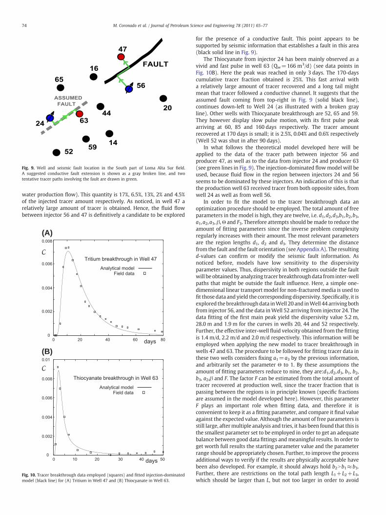
Fig. 9. Well and seismic fault location in the South part of Loma Alta Sur field.A suggested conductive fault extension is shown as a gray broken line, and twotentative tracer paths involving the fault are drawn in green.

74 M. Coronado et al. / Journal of Petroleum Science and Engineering 78 (2011) 65–77

water production flow). This quantity is 17%, 6.5%, 13%, 2% and 4.5%of the injected tracer amount respectively. As noticed, in well 47 arelatively large amount of tracer is obtained. Hence, the fluid flowbetween injector 56 and 47 is definitively a candidate to be explored

(A)

(B)

Fig. 10. Tracer breakthrough data employed (squares) and fitted injection-dominatedmodel (black line) for (A) Tritium in Well 47 and (B) Thiocyanate in Well 63.

for the presence of a conductive fault. This point appears to besupported by seismic information that establishes a fault in this area(black solid line in Fig. 9).

The Thiocyanate from injector 24 has been mainly observed as avivid and fast pulse in well 63 (Qw=166 m3/d) (see data points inFig. 10B). Here the peak was reached in only 3 days. The 170-dayscumulative tracer fraction obtained is 25%. This fast arrival witha relatively large amount of tracer recovered and a long tail mightmean that tracer followed a conductive channel. It suggests that theassumed fault coming from top-right in Fig. 9 (solid black line),continues down-left to Well 24 (as illustrated with a broken grayline). Other wells with Thiocyanate breakthrough are 52, 65 and 59.They however display slow pulse motion, with its first pulse peakarriving at 60, 85 and 160 days respectively. The tracer amountrecovered at 170 days is small; it is 2.5%, 0.04% and 0.6% respectively(Well 52 was shut in after 90 days).

In what follows the theoretical model developed here will beapplied to the data of the tracer path between injector 56 andproducer 47, as well as to the data from injector 24 and producer 63(see green lines in Fig. 9). The injection-dominated flowmodel will beused, because fluid flow in the region between injectors 24 and 56seems to be dominated by these injectors. An indication of this is thatthe production well 63 received tracer from both opposite sides, fromwell 24 as well as from well 56.

In order to fit the model to the tracer breakthrough data anoptimization procedure should be employed. The total amount of freeparameters in the model is high, they are twelve, i.e. d1,d2,d3,b1,b2,b3,a1,a2,a3, β,Θ and F3. Therefore attempts should bemade to reduce theamount of fitting parameters since the inverse problem complexityregularly increases with their amount. The most relevant parametersare the region lengths d1, d2 and d3. They determine the distancefrom the fault and the fault orientation (see Appendix A). The resultingd-values can confirm or modify the seismic fault information. Asnoticed before, models have low sensitivity to the dispersivityparameter values. Thus, dispersivity in both regions outside the faultwill be obtainedby analyzing tracer breakthroughdata from inter-wellpaths that might be outside the fault influence. Here, a simple one-dimensional linear transportmodel for non-fracturedmedia is used tofit those data and yield the corresponding dispersivity. Specifically, it isexplored the breakthroughdata inWell 20 and inWell 44 arriving bothfrom injector 56, and the data inWell 52 arriving from injector 24. Thedata fitting of the first main peak yield the dispersivity value 5.2 m,28.0 m and 1.9 m for the curves in wells 20, 44 and 52 respectively.Further, the effective inter-well fluid velocity obtained from the fittingis 1.4 m/d, 2.2 m/d and 2.0 m/d respectively. This information will beemployed when applying the new model to tracer breakthrough inwells 47 and 63. The procedure to be followed for fitting tracer data inthese two wells considers fixing a1=a3 by the previous information,and arbitrarily set the parameter Θ to 1. By these assumptions theamount of fitting parameters reduce to nine, they are:d1,d2,d3, b1, b2,b3, a2,β and F. The factor F can be estimated from the total amount oftracer recovered at production well, since the tracer fraction that ispassing between the regions is in principle known (specific fractionsare assumed in the model developed here). However, this parameterF plays an important role when fitting data, and therefore it isconvenient to keep it as a fitting parameter, and compare it final valueagainst the expected value. Although the amount of free parameters isstill large, aftermultiple analysis and tries, it has been found that this isthe smallest parameter set to be employed in order to get an adequatebalance between good data fittings andmeaningful results. In order toget worth full results the starting parameter value and the parameterrange should be appropriately chosen. Further, to improve the processadditional ways to verify if the results are physically acceptable havebeen also developed. For example, it should always hold b2Nb1≈b3.Further, there are restrictions on the total path length L1+L2+L3,which should be larger than L, but not too larger in order to avoid

75M. Coronado et al. / Journal of Petroleum Science and Engineering 78 (2011) 65–77

paths sections that go in the opposite direction to the productionwell (i.e. angle ζ described in the Appendix A should be smallerthan 90o). Another restriction is that the sum of the fluid transittime in each regionT1+T2+T3, here Ti≡Li/ui, should be similar oracceptably smaller than the average tracer transit time tT. Theseconditions should hold in order to accept a solution from theoptimization procedure.

In the next sections the optimization procedure and the fitting ofthe analytical model developed here to the tracer breakthrough datafrom Well 47 and Well 63 is described. In order to perform the fittingit is first necessary to transform the time data to the dimensionlesstime variable used in the model, i.e. tD= t/tT. Tracer concentration iskept in its original dimensions (therefore the fitting parameter F3 isin reality F3CREF). These original dimensions are relative concentra-tion, it means: tracer concentration (amount/m3) times water flow atproduction well (m3/day) times (1 day) divided by the total injectedtracer amount.

6.1. The optimization procedure

In describing the optimization procedure to determine the modelparameters, it is important to remark that inverse problems areregularly ill-posed. This means that a solution not always exists, thatmultiple solutions are possible, or also that small variations on theoriginal data can yield large fitting parameters modifications (Menke,1984). This issue should be kept in mind when treating the Loma AltaSur data. The optimization procedure employed to estimate themodelparameters consists in the minimization of an objective functioncomposed by the standard direct sum the squared differencesbetween data points and model predictions. The obtained objectivefunction is highly non-linear, and the method employed to minimizeit is Levenberg–Marquardt. This method is used since it has proven tobe reliable and efficient in solving similar problems, and it easilyallows the introduction of restrictions on the parameter values. Inorder to reduce uncertainty andmitigate the solution non-uniquenessproblem adequate starting values as well as tight search parameterdomains should be provided. The amount of free parameters finallyemployed is eight plus the linear parameter F3.

6.2. The tracer path between injector 56 and production well 47

The straight line surface distance joining wells 47 and 56 is 133 m.The tracer transit time obtained from the tracer breakthrough dataconsidering only times lower than 80 days (first pulse arrival period) is⟨t⟩=23.8 days; thus, the effective tracer pulse velocity is 5.6 m/d. Byusing the dispersivity obtained from the nearby Well 44 data(α=28.0 m), it yields the parameter value a1=a3=0.210. This valuetogether with Θ=1 will be employed as fix parameters in theoptimization procedure. The starting parameter value for b1 and b3 isextracted from the fluid velocity obtained in Well 44 (2.2 m/d). Itfollowsb1≈b3≈0.4. Startingparameters fordi canbeobtained fromthecorresponding suggested path in the map of Fig. 9. It follows d1≈0.52,d2≈0.42 and d3≈0.38. Other starting parameter values employed areβ=1, a2=0.2 and b2=10. The parameter domains finally establishedfor the lengths are 0.15≤d1≤0.6, 0.4≤d2≤0.8 and 0.15≤d3≤0.8. Forvelocities the range is 0.1≤b1≤1.2 0.1≤b2≤20 and 0.1≤b3≤1.2, forfault dispersion it is 0.02≤a2≤0.7, and for β it was taken 0.2≤β≤1.5.No starting value or parameter range are needed for F3.

The optimization procedure applied to data points for times lowerthan 80 days yields good results, as shown in the curve of Fig. 10A.The parameters found are the following: d1=0.425, d2=0.490,d3=0.241, a2=0.0423,b1=1.090, b2=9.841, b3=1.198, β=0.490and F3=0.027. The objective function is 3.84×10−6 (21 data points).Sensitivity plots of the objective function dependence on each of theeight fitting parameters show that indeed the solution is a localminimum. The optimum parameter values yield L1=56.5 m, L2=

91.5m, L3=32.1m. The dispersivity in Region 2 becomes α2=5.6m.The fluid velocities are u1=6.1 m/d, u2=55.0m/d and u3=6.7m/d.The effect of fluid matrix on the fracture network in Region 2is noticeable since β≈0.5. The total tracer path length is L1+L2+L3=180.0m. The fluid total transit time T1+T2+T3 is 15.7 days,which is acceptable smaller than the tracer transit time 23.8 days, asexpected. The velocity in the fault region is approximately 9 timesgreater than the velocity outside the fault. The longitudinal dispersioncoefficient D=αu in the fracture network of the fault is 309 m2/d,which is twice the dispersion in the regions outside the fault.

One of the most significant applications of the model, beyonddetermining fault flow properties, is its capacity to estimate faultorientation. From the values L1, L2 and L3 the angle Ω that forms thefault line and the straight line joining the injection-production wellscan be calculated, as described in the Appendix A. In this case theangle is Ω=41.5°. This angle is approximately similar to the angledisplayed in Fig. 9 (obtained from Badessich et al., 2005), which isapproximately 66°. This would indicate that the fault has a higherslope at that region. The path angle at the junction L1 to L2and L2 to L3is ς=84.7°, which means the flow arriving or leaving the fault isalmost perpendicular to the fault. By applying the fault-dominatedflow model a smaller fault orientation angle follows, it is Ω=29.1°.

6.3. The tracer path between injector 24 and production well 63

The original data show an exceptional horizontal long tail(Badessich et al., 2005). It certainly comes from a phenomenon thatis not taken into account in this new model. Consequently, onlydata for times lower than 50 days are considered. Also, all data arearbitrarily shifted downwards to eliminate the long constant tail. Bythis way the lowest data point in the tail becomes zero (see datapoints in Fig. 10B). The dimensionless parameters to be used in themodel are associated to the inter-well distance, L=118m, the tracertransit time tT=10.3d, and the average tracer velocity L/tT which is11.4 m/d. The dispersivity for Regions 1 and 3 is taken as an averagebetween the dispersivity values obtained from the data from wells20 and 52. This means α=3.6m and therefore a1=a3=0.030 isset, together with Θ=1. After diverse searches the selected startingparameters were d1=0.3, d2=0.88 and d3=0.53, together withb1=b3=0.15, a2=0.5, b2=10 and β=1. The parameter domaintaken was 0.001≤d1≤0.6, 0.6≤d2≤1, 0.001≤d3≤0.8 0.2≤b1≤1.3,0.1≤b2≤20, 0.2≤b3 ≤1.5 and 0.3≤a2≤0.9, 0.5≤β≤1.5.

The optimization procedure yields a good result. It shows the curvedisplayed in Fig. 10B, with an objective function value of 2.3×10−6(14data points) and the following parameters: d1=0.018, d2=0.951,d3=0.166, a2=0.678, b1=1.221, b2=3.534, b3= 1.468, β=0.805 andF3=0.019. Sensitivity plots of the objective function (Dai and Samper,2004) on all fitting parameters show that the solution corresponds toa local minimum. This is illustrated in Fig. 11, where the objectivefunction is plotted with respect to each one of the dimensionlessparameters in the same x-axes. All curves show a parabola-type curvewith a minimum at the optimum value. The resulting dimensionalvariables are L1=2.1m, L2=112.2 m, L3=19.6 m. From these data it isto be observed that the fault passes very close to the injection well.Dispersivity in Region 2 isα2=80.0 m. The velocities are u1=13.9m/d,u2=40.4m/d,u3=16.8m/d. The effect of diffusion in the matrixof the fracture network yields β=0.80. The total tracer path length isL1+L2+L3=133.9 m.Thefluid total transit time T1+T2+T3 is 4.1 days.The longitudinal dispersion coefficient is 3230m2/din the fault regionand only 60 m2/d in the regions outside the fault.

The fault orientation angle isΩ=10.4°, which is a very small slopewith respect the joining line between wells 24 and 63. Anyway, theresults lead to the conclusion that the fault betweenwells 24 and 63 isprobably a continuation of the fault shown at the top right side inFig. 9, determined by seismic information (Badessich, et al., 2005). Thefault arrival angle isς=79.8°. By employing the other model flow

Fig. 11. Sensitivity plots of the objective function in terms of the eight fittingdimensionless parameters around its optimum value.

76 M. Coronado et al. / Journal of Petroleum Science and Engineering 78 (2011) 65–77

case, i.e. the fault-dominated flow, a very similar orientation angle,Ω=10.5° is obtained.

Another possibility is that the fault does not cross between wells24 and 63, but it passes close over both of them. In this case Eqs. (A3)and (A4) from the Appendix A with L3NL1 applies. These equationsare solved analytically considering a small angle Ω, i.e.cos Ω≈1.It follows Ω=8.3° (confirmed graphically) and ς=76.9°. Thus, thisfault location is another possible solution, which is also very similarto the previous solution.

7. Summary and conclusions

An analytical tracer transport model has been developed in orderto describe inter-well tracer tests in the case when a reservoir hasconductive geological faults. It considers a system composed by threecoupled regions with different properties. The first region representsthe tracer path from the injector to the fault, the second region thepath along the fault, and the third one, the region from the fault tothe production well. Main physics phenomena involved are advectionand hydrodynamic dispersion. This model generalizes a previousanalytical model developed for the case when the fault system hasno external fluid flows. A mathematical procedure has now beendesigned in order to consider the presence of possible external flows.It consists in considering the three mentioned regions as independentbut coupled by effective sequential tracer sources. Additionally, thenew model incorporates the important feature that the faultcomprehends a fracture network. This fact is introduced by applyinga standard double-porosity formalism for the fault region. Further, theDanckwert's boundary condition is set at the production well in thethird region, which establishes that no dispersive flow appears atthis border. Two different fault flow situations are examined. Onesituation is when the reservoir fluid arrives in the fault region fromexternal sources. The fluid moves along the fault and leaves it at theopposite fault end. In this case the fluid from the injector reaches thefault without affecting the flow inside it (fault-dominated flow). Othersituation is when the injector determines the flow direction in thefault (injection-dominated flow). In this case the fluid from the injectorgets into the fault and at that point makes the fluid to flow in oppositefault directions, leaving the fault at both ends. These two patternsplay the role of limiting situations. Thus, an intermediate case wouldyield a tracer breakthrough curve that presumable falls between thesetwo corresponding curves. The equation set is analytically solved inLaplace space and the inverse calculated numerically by the Stehfestalgorithm. The total amount of model parameters is 12, which is alarge parameter number when fitting a model to real data. Analysesweremade in order to reduce this amount by incorporating additionalsystem information. In this context, it is also of great help to know thesensitivity of the tracer breakthrough curve to each of the relevant

parameters. A high sensitivity to the path length in each region and tothe velocity along the fault has been found. Marginal sensitivity (i.e.sensitivity only at low fluid velocity in the fault) was foundwith respectto the two parameters associated to the interaction matrix-fracturenetwork. This is probably due to the fact that at highfluid speeds there isnot enough time for this interaction to take place. Low sensitivity isfound to the dispersivity in the system. The breakthrough curves displaygreat similarity in shape for the two fault flow cases examined(injection-dominated and fault-dominated). The former case showstracer concentrations that are close to the half of the concentrations inthe latter case. This relays on the fact that approximately half of thetracer moves in the opposite direction of the production well and getslost from the fault system. The previous existingmodel for a closed faultyields tracer breakthrough curves that in general fall between the curvesof the twocases considered in thenewmodel. These factsmight indicatethat the three cases capture the samemain effective phenomena of thetracer transport in the system , and by using just one of them anapproximate general overview of it can be obtained (care should betaken with the interpretation of the linear parameter associated to thetracermass). In this case, and due to its relativemathematical simplicityand the physics phenomena included, the usage of the injection-dominated flow solution is suggested. A remarkable and highlytranscendental feature of the model developed here is its capability todetermine the fault orientation. This fact canbeof great help to reservoirengineers when setting up a reservoir geological model.

An application of the model developed here was made to areservoir tracer test performed in the Loma Alta Sur field in Argentina,which has been documented in the open literature. Here, tracertests and seismic information indicate the presence of conductivefaults. To apply the new model two field tracer breakthrough curveswere selected. The optimization procedure has been very carefullyexamined and applied. The fault orientation is obtained fromthe analysis, which closely reproduces the reported orientationestablished by seismic information. Even more, a continuation of thereported fault beyond the area originally considered is concluded.

Acknowledgments

We acknowledge Prof. C. Somaruga from the Universidad Nacionaldel Comahue, Argentina for highlighting comments on the Loma AltaSur tracer test.We also thank R.P. Everitt for revising the English in themanuscript.

Appendix A. Determination of the fault orientation

In this section a method to obtain fault orientation informationfrom a given data set {L1,L2,L3}is described. Specifically as shown inFig. 9, a determination of the orientation angle Ω, formed by the faultand the line joining the injection and production well can be done.Graphically, this angle results from placing a circle of radius L1 and L3around the corresponding injection and production well, and thenintroducing L2 in such a way that the length L2 properly joints the twocircles, as displayed in the mentioned figure.

An analytical expression for the angleΩ can be obtained if L1,L2 andL3 are known. This expression can be derived from examining thegeneral situation displayed in Fig. 10, where the path fromRegion 1 donot go perpendicular to the fault line, but forming an angle ς. The sameangle is assumed for the path from the fault to the production well. Byperforming a geometrical analysis a relation between the tracer pathand the inter-well direct line Lis obtained in terms of di=Li/L as

d1 + d3ð Þ2 + d22 + 2d2 d1 + d3ð Þcos ς = 1; ðA1Þ

and the fault orientation angle Ω by

sinΩ = d1 + d3ð Þ sinς ðA2Þ

(A) (B)

Fig. A-3. The cases where the fault crosses the well-joining-line outside the inter-wellregion.

77M. Coronado et al. / Journal of Petroleum Science and Engineering 78 (2011) 65–77

The procedure to determine Ω consists in obtaining ς fromEq. (A1) and then evaluating Ω from Eq. (A2).

A different situation appears when fault crosses the injector–producer joining line outside the inter-well region. This situation isillustrated in Fig. 11, and two cases are displayed. Themodel developedin this paper also applies. In case (A) L1NL3 and in case (B) L1bL3. Insituation (A) it holds

sinΩ = d1−d3ð Þ sinς ðA3Þ

d21 sin2 ς + d1 + d3ð Þ cosς + d2 +d3

d1−d3cosΩ

� �2=

d1d1−d3

� �2

ðA4ÞFrom Eqs. (A3) and (A4) the fault orientation angle Ω and the

angle ς can be evaluated. In case (B), when d1bd3, the same equationshold but interchanging d1 and d3.

Fig. A-1. Schematic description of fault orientation.

Fig. A-2. Geometry of the tracer path.

References

Badessich, M.F., Swinnen, I., Somaruga, C., 2005. The use of tracers to characterize highlyheterogeneous fluvial reservoirs: field results. 2005 SPE International Symposiumon Oilfield Chemistry, Houston 2–4 February, 2005. SPE e-library paper 92030,Richardson TX.

Bense, V.F., Person, M.A., 2006. Faults as conduit-barrier system to fluid flow insiliciclastic sedimentary aquifers. Water Resour. Res. 42, W05421. doi:10.1029/2005 WR004480.

Caine, J.S., Evans, J.P., Forster, C.B., 1996. Fault zone architecture and permeabilitystructure. Geology 24 (11), 1025–1028.

Coronado, M., Ramírez-Sabag, J., 2008. Analytical model for tracer transport inreservoirs having a conductive geological fault. J. Pet. Sci. Eng. 62, 73–79.

Coronado, M., Ramírez-Sabag, J., Valdiviezo-Mijangos, O., 2007. On the boundaryconditions in tracer transportmodels for fractured porous underground formations.Rev. Mex. Fís. 53 (4), 260–269.

Dai, Z., Samper, J., 2004. Inverse problem of multi-component reactive chemicaltransport in porous media: formulation and applications. Water Resour. Res. 40,W0747-1. doi:10.1029/2004 WR003248.

Fairley, J.P., Hinds, J.J., 2004. Field observation of fluid circulation patterns in a normalfault system. Geophys. Res. Lett. 31 (L19502), 1–4. doi:10.1029/2004GL020812.

Houseworth, J.E., 2004. An analytical model for solute transport in unsaturated flowthrough a single fracture and porous rock matrix. Lawrence Berkeley NationalLaboratory. paper LBNL-56342. http://repositories.cdlib.org/lbnl/LBNL-56342.

Maloszewski, P., Zuber, A., 1985. On the theory of tracer experiments in fissured rockswith a porous matrix. J. Hydrol. 79, 333–358.

Menke, W., 1984. Geophysical data analysis: discrete inverse theory. Academic PressInc., Orlando.

Schwartz, R.C., McInnes, K.J., Juo, A.S.R., Wilding, L.P., Reddell, D.L., 1999. Boundaryeffects on solute transport in finite soil columns. Water Resour. Res. 35, 671–681.