arX

iv:1

305.

1907

v2 [

hep-

th]

12

Aug

201

3

Double Field Theory:

A Pedagogical Review

Gerardo Aldazabala,b, Diego Marquesc and Carmen Nunezc,d

aCentro Atomico Bariloche, bInstituto Balseiro (CNEA-UNC) and CONICET.

8400 S.C. de Bariloche, Argentina.

cInstituto de Astronomıa y Fısica del Espacio (CONICET-UBA)

C.C. 67 - Suc. 28, 1428 Buenos Aires, Argentina.

dDepartamento de Fısica, FCEN, Universidad de Buenos Aires

aldazaba@cab.cnea.gov.ar , diegomarques@iafe.uba.ar , carmen@iafe.uba.ar

Abstract

Double Field Theory (DFT) is a proposal to incorporate T-duality, a distinctive sym-

metry of string theory, as a symmetry of a field theory defined on a double configuration

space. The aim of this review is to provide a pedagogical presentation of DFT and its ap-

plications. We first introduce some basic ideas on T-duality and supergravity in order to

proceed to the construction of generalized diffeomorphisms and an invariant action on the

double space. Steps towards the construction of a geometry on the double space are dis-

cussed. We then address generalized Scherk-Schwarz compactifications of DFT and their

connection to gauged supergravity and flux compactifications. We also discuss U-duality

extensions, and present a brief parcours on world-sheet approaches to DFT. Finally, we

provide a summary of other developments and applications that are not discussed in detail

in the review.

August 13, 2013

Contents

1 Introduction 3

2 Some references and a guide to the review 8

3 Double Field Theory 11

3.1 T-duality basics . . . . . . . . . . . . . . . . . . . . . . . . . . . . . . . . . . . . . 11

3.2 Supergravity basics . . . . . . . . . . . . . . . . . . . . . . . . . . . . . . . . . . . 16

3.3 Double space and generalized fields . . . . . . . . . . . . . . . . . . . . . . . . . . 17

3.4 Generalized Lie derivative . . . . . . . . . . . . . . . . . . . . . . . . . . . . . . . 21

3.5 Consistency constraints . . . . . . . . . . . . . . . . . . . . . . . . . . . . . . . . 23

3.6 The action . . . . . . . . . . . . . . . . . . . . . . . . . . . . . . . . . . . . . . . . 25

3.7 Equations of motion . . . . . . . . . . . . . . . . . . . . . . . . . . . . . . . . . . 29

4 Double Geometry 32

4.1 Riemannian geometry basics . . . . . . . . . . . . . . . . . . . . . . . . . . . . . . 32

4.2 Generalized connections and torsion . . . . . . . . . . . . . . . . . . . . . . . . . 35

4.3 Generalized curvature . . . . . . . . . . . . . . . . . . . . . . . . . . . . . . . . . 39

4.4 Generalized Bianchi identities . . . . . . . . . . . . . . . . . . . . . . . . . . . . . 43

5 Dimensional reductions 44

5.1 Scherk-Schwarz compactifications . . . . . . . . . . . . . . . . . . . . . . . . . . . 44

5.2 Geometric fluxes . . . . . . . . . . . . . . . . . . . . . . . . . . . . . . . . . . . . 49

5.3 Gauged supergravities and duality orbits . . . . . . . . . . . . . . . . . . . . . . . 53

5.4 Generalized Scherk-Schwarz compactifications . . . . . . . . . . . . . . . . . . . . 58

5.5 From gauged DFT to gauged supergravity . . . . . . . . . . . . . . . . . . . . . . 62

5.6 Duality orbits of non-geometric fluxes . . . . . . . . . . . . . . . . . . . . . . . . 63

1

6 U-duality and extended geometry 70

6.1 Generalized diffeomorphisms and the section condition . . . . . . . . . . . . . . . 70

6.2 The E7(7) case and maximal gauged supergravity . . . . . . . . . . . . . . . . . . 73

7 Worldsheet motivations and approaches to DFT 80

7.1 The string spacetime action . . . . . . . . . . . . . . . . . . . . . . . . . . . . . . 80

7.2 Double string sigma model . . . . . . . . . . . . . . . . . . . . . . . . . . . . . . . 82

7.3 DFT from the double sigma model . . . . . . . . . . . . . . . . . . . . . . . . . . 87

8 Other developments and applications 91

8.1 Non-commutative/non-associative structures in closed string theory . . . . . . . 91

8.2 Large gauge transformations in DFT . . . . . . . . . . . . . . . . . . . . . . . . . 93

8.3 New perspectives on α′ corrections . . . . . . . . . . . . . . . . . . . . . . . . . . 94

8.4 Geometry for non-geometry . . . . . . . . . . . . . . . . . . . . . . . . . . . . . . 95

8.5 Beyond supergravity: DFT without strong constraint . . . . . . . . . . . . . . . . 96

8.6 (Exotic) brane orbits in DFT . . . . . . . . . . . . . . . . . . . . . . . . . . . . . 97

8.7 New possibilities for upliftings, moduli fixing and dS vacua . . . . . . . . . . . . 98

9 Acknowledgments 98

2

1 Introduction

Double Field Theory (DFT) [1, 2] is a proposal to incorporate T-duality, a distinctive

symmetry of string (or M-)theory, as a symmetry of a field theory. At first sight, such

attempt could appear to lead to a blind alley since the very presence of T-duality re-

quires extended objects like strings which, unlike field theory particles, are able to wrap

non-contractible cycles. It is the very existence of winding modes (associated to these

wrappings) and momentum modes that underlies T-duality, which manifests itself by con-

necting the physics of strings defined on geometrically very different backgrounds. Then,

a T-duality symmetric field theory must take information about windings into account.

A way to incorporate such information is suggested by compactification of strings on

a torus. In string toroidal compactifications, there are compact momentum modes, dual

to compact coordinates ym, m = 1, . . . , n, as well as string winding modes. Therefore,

it appears that a new set of coordinates ym, dual to windings, should be considered for

the compactified sector in the field theory description. It is in this sense that DFT is a

“doubled” theory: it doubles the coordinates of the compact space. Formally, the non-

compact directions xµ, µ = 1, . . . , d are also assigned duals xµ for completion, although

this is merely aesthetical since nothing really depends on them. The DFT proposal is

that, for aD-dimensional space with d non-compact space-time dimensions and n compact

dimensions, i.e. D = n+d, the fields depend on coordinates XM = (xµ, ym, xµ, ym), where

xµ are space-time coordinates, xµ are there simply for decoration, and YA = (ym, y

m) are

2n compact coordinates, with A = 1, . . . , 2n.

When the compactification scale is much bigger than the string size, it is hard for

strings to wrap cycles and winding modes are ineffective at low energies. In the DFT

framework, this corresponds to the usual situation where there is no dependence on dual

coordinates. Oppositely, in the T-dual description, if the compactification scale is small,

then the momentum (winding) modes are heavy (light), and DFT only depends on dual

coordinates. Either way, these (de)compactification limits typically amount on the DFT

side to constrain the theory to depend only on a subset of coordinates. In particular, when

all the coordinates are non-compact, one finds complete correspondence with supergravity

3

in D = 10 dimensions.

The T-duality group associated to string toroidal compactifications on T n is O(n, n).

The doubled internal coordinates YA mix (span a vector representation) under the action

of this group. However, it proves useful to formulate the theory in a double space with full

duality group O(D,D), where all D coordinates are doubled, mimicking a string theory

where all dimensions are compact.1

The next step in the construction of DFT is to choose the defining fields. In the

simplest formulation of DFT, the field content involves the D-dimensional metric gij, a

two-form field bij and a scalar dilaton field φ. From a string perspective, they correspond

to the universal gravitational massless bosonic sector, present in the bosonic, heterotic

and Type II string theories as well as in the closed sector of Type I strings, in which

case bij would be a Ramond-Ramond (R-R) field. However, since we are looking for an

O(D,D) invariant theory, the fundamental fields should be O(D,D) tensors with 2D

dimensional indices. In fact, in DFT the gij and bij fields are unified in a single object:

a generalized O(D,D) symmetric metric HMN , with M,N = 1, . . . , 2D, defined in the

double space. Then, based on symmetries, DFT unifies through geometrization, since it

incorporates the two-form into a generalized geometric picture. There is also a field d,

which is a T-scalar combining the dilaton φ and the determinant of the metric g. The

first part of this review will be dedicated to discuss the consistent construction of a DFT

action as a functional of these generalized fields on a doubled configuration space.

In the decompactification limit (taking for example D = 10 so as to make contact with

string theory), when the dual coordinates are projected out, the DFT action reproduces

the action of the universal massless bosonic sector of supergravity

S =

∫dx√ge−2φ

(R + 4 (∂φ)2 − 1

12HijkH

ijk

),

where Hijk = 3∂[ibjk] is the field strength of the two-form. This limit action is invariant

under the usual diffeomorphisms of General Relativity and gauge transformations of the

two-form. Following with the unification route, we then expect to combine these trans-

1 Time is treated here at the same level of other space coordinates for simplicity, but it can be restored

by a standard Wick rotation.

4

formations into “generalized diffeomorphisms” under which the DFT action should be

invariant. They should then reduce to standard general coordinate and gauge transfor-

mations in the decompactification limit. In Section 3 we will define these transformations

and discuss constraint equations required by gauge consistency of the generalized diffeo-

morphisms. Generically, these constraints restrict the space of configurations for which

DFT is a consistent theory, i.e. DFT is a restricted theory.

The constraints of the theory are solved in particular when a section condition or

strong constraint, is imposed. This restriction was proposed in the original formulations

of DFT, inspired by string field theory constraints. It implies that the fields of the theory

only depend on a slice of the double space parameterized by half of the coordinates, such

that there always exists a frame in which, locally, the configurations do not depend on the

dual coordinates. Since the strong constraint is covariant under the global symmetries,

the theory can still be covariantly formulated, but it is actually not truly doubled after it

is solved.

Nevertheless, one can also find other solutions to the constraints that violate the strong

constraint. In particular, Scherk-Schwarz (SS) dimensional reductions of DFT, where the

space-time fields are twisted by functions of the internal coordinates, have proven to be

interesting scenarios where consistent strong-constraint violating configurations are al-

lowed. Interestingly enough, the SS reduction of (bosonic) DFT on the doubled space

leads to an action that can be identified with (part of) the action of the bosonic sector of

four-dimensional half-maximal gauged supergravities. Recall that gauged supergravities

are deformations of ordinary abelian supergravity theories, in which the deformation pa-

rameters (gaugings) are encoded in the embedding tensor. DFT provides a higher dimen-

sional interpretation of these gaugings in terms of SS double T-duality twists. Moreover,

the quadratic constraints on gaugings are in one to one correspondence with the closure

constraints of the generalized diffeomorphisms.

Gauged supergravities describe superstring compactifications with fluxes, where the

gaugings correspond to the quantized fluxes. Therefore it is instructive to look at the con-

nection between SS reductions of DFT and string flux compactifications. This connection

5

is subtle. It is known that orientifold compactifications of D = 10 effective supergravity

actions, corresponding to the low energy limit of string theories, lead to four dimensional

superpotentials in which the coefficients are the fluxes. However, by looking at flux com-

pactifications of string theories, expected to be T-duality related (for instance, type IIA

and type IIB theories) the effective superpotentials turn out not to be T-dual. Namely,

these compactifications are gauged supergravities but with different orbits of gaugings

turned on, not connected by T-duality. By invoking symmetry arguments, it has been

suggested that new fluxes should be included in order for the full superpotentials to be

T-duals, so as to repair the mismatch. Similarly, more fluxes are required by invoking

type IIB S-duality, M-theory or heterotic/type I S-duality, etc. Then, by imposing du-

ality invariance at the level of the four dimensional effective theory, the full (orientifold

truncated) supergravity theory is obtained with all allowed gaugings.

Hence, we can conclude that four dimensional gauged supergravity incorporates stringy

information that, generically, is not present in the reduction of a ten dimensional effective

supergravity action. Compactification of DFT contains this stringy information from

the start and provides a geometric interpretation for fluxes, even for those that are non-

geometric from a supergravity point of view.

There have also been different proposals to extend DFT ideas to incorporate the full

stringy U-duality symmetry group. Take E7(7) as an example, which includes T-dualities

and strong-weak duality. The symmetrization now requires an Extended Geometry on

which one can define an Extended Field Theory (EFT). Interestingly enough, from a

string theory perspective such formulation automatically incorporates information on NS-

NS and R-R fields. While in DFT with O(n, n) symmetry a doubled 2n compactified

space is needed, in EFT coordinates span a mega-space with more dimensions, where SS

compactifications lead to four-dimensional gauged maximal supergravity.

Closely related to DFT (or EFT) is the framework of Generalized Geometry (or Ex-

ceptional Generalized Geometry), a program that also incorporates duality as a building

block. In Generalized Geometry (GG), the tangent space, where the vectors generat-

ing diffeomorphisms live, is enlarged to include the one-forms corresponding to gauge

6

transformations of the two-form. The internal space is not extended, but the notion of

geometry is still modified. DFT and GG are related when the section condition (which

un-doubles the double space) is imposed.

To summarize, DFT is a T-duality invariant reformulation of supergravity which ap-

pears to offer a way to go beyond the supergravity limits of string theory by introducing

some stringy features into particle physics. DFT is all about T-duality symmetries, uni-

fication and geometry. It is a rather young theory, still under development, but it has

already produced plenty of new perspectives and results. There are still many things to

understand, and the number of applications is increasing. Here we intend to review this

beautiful theory and some of its applications, in as much a pedagogical fashion as we can.

7

2 Some references and a guide to the review

In this review we intend to provide a self-contained pedagogical introduction to DFT.

We will introduce the basics of the theory in lecture-like fashion, mostly intended for

non-experts that are willing to know more about this fascinating theory. We will mainly

review the recent literature on the formulation and applications of the theory. The field

is undergoing a quick expansion, and many exciting results are still to appear. Given

the huge amount of material in this active area of research, we are forced to leave out

many developments that are as important and stimulating as those that we consider

here. With the purpose of reducing the impact of this restriction, we provide an updated

list of references, were the reader can find more specific information. We apologize if,

unintentionally, we have omitted important references.

Let us first start with a brief list of books on string theory [3]. There are already

some very good and complete reviews and lectures on this and related topics, that we

strongly suggest. In [4, 5] the reader will find a complete exposition on T-duality. Flux

compactifications are nicely reviewed in [6]. Comprehensive reports on non-geometric

fluxes and their relation to gauged supergravities are those in [7] and [8], respectively.

DFT has also been reviewed in [9], and Generalized Geometry in [10]. A complete review

on duality symmetric string and M-theory can be found in [11].

Historically, the idea of implementing T-duality as a manifest symmetry goes back

to M. Duff [12] and A. Tseytlin [13], where many of the building blocks of DFT were

introduced. In [12], one can identify already the double coordinates, the generalized

metric and frame, the notion of duality symmetric sigma models and the extension of

these concepts to U-duality. In [13], the idea of DFT was essentially present: double

coordinates were considered, an effective action for the metric in double space presented,

and the necessity of consistency constraints noted. Soon after, Siegel contributed his

pioneer work [1], in which a full duality symmetric action for the low-energy superstring

was built in superspace formalism. More recently, C. Hull and B. Zwiebach combined

their expertise on double geometry [14] and string field theory [15] to build Double Field

Theory [2]. Later, together with O. Hohm, they constructed a background independent

8

[16] and generalized metric [17] formulation of the theory. The relation of their work

to Siegel’s was analyzed in [18]. Closely related to DFT is the Generalized Geometry

introduced by N. Hitchin and M. Gualtieri [19] and related to string theory in the works

by M. Grana, T. Grimm, J. Louis, L. Martucci, R. Minasian, M. Petrini, A. Tomasiello

and D. Waldram [20], among others.

The inclusion of heterotic vector fields in the theory was discussed in [21] (see also

[22]). R-R fields and a unification of Type II theories were included in [23, 24, 25], while

the massive Type II theory was treated in [26]. The inclusion of fermions and super-

symmetrization was performed in [27, 24]. There are many works devoted to explore the

geometry of DFT [28, 24, 29, 30]. A fully covariant supersymmetric Type II formulation

was constructed by I. Jeon, K. Lee and J. Park in [31]. The gauge symmetries and equa-

tions of motion were analyzed by S. Kwak [32], and the gauge algebra and constraints of

the theory were discussed in [33, 34]. The connection with duality symmetric non-linear

sigma models was established by D. Berman, N. Copland and D. Thompson in [35, 36, 37].

Many of these works were inspired by Siegel’s construction [1].

Covariant frameworks extending T-duality to the full U-duality group were built as

well. These include works by C. Hull [38], P. Pacheco and D. Waldram [39], D. Berman

and M. Perry [40], the E11 program by P. West et. al. [41] and [42, 43]. More recent DFT-

related developments can be found in [44, 45, 46, 47, 48, 49, 50, 51]. Also in this direction,

but more related to non-geometry and gauged supergravities we have [52, 53, 54, 55].

The ideas introduced in [56, 57, 58, 59] led to the development of non-geometry, and

T-dual non-geometric fluxes were named as such in [60] (see also [61]). Later, S-dual

fluxes were introduced in [62], and finally the full U-dual set of fluxes was completed in

[52]. Fluxes were considered from a generalized geometrical point of view in [20], and also

from a double geometrical point of view in [14, 63, 64]. The relation between DFT, non-

geometry and gauged supergravities was explored in [65, 66, 67, 68, 69, 70, 71, 72, 73, 74].

Different world-sheet perspectives for fluxes were addressed in [75, 76, 77].

Some other developments on DFT and related works can be found in [78]. In the final

section we include more references, further developments and applications of DFT.

9

The present review covers the following topics:

• Section 3 provides a general introduction to DFT. Starting with some basics on

T-duality as a motivation, double space and generalized fields are then defined.

A generalized Lie derivative encoding usual diffeomorphisms and two-form gauge

transformations is introduced, together with its consistency constraints. We then

present the DFT action, its symmetries and equations of motion.

• Section 4 reviews the construction of an underlying double geometry for DFT.

Generalized connections, torsion, and curvatures are discussed, and their similarities

and differences with ordinary Riemannian geometry are examined.

• Section 5 is devoted to a discussion of dimensional reductions of DFT. After a brief

introduction of usual SS compactifications, the procedure is applied to deal with gen-

eralized SS compactifications of DFT. The notions of geometric and non-geometric

fluxes are addressed and the connection with gauged supergravity is established.

• Section 6 considers the U-duality extension of DFT, Extended Geometries, Ex-

tended Field Theories and their relation to maximal gauged supergravity.

• Section 7 reviews the various attempts to construct O(D,D) invariant non-linear

sigma models, and their relation to DFT.

• Section 8 provides a brief summary of different developments related to DFT (and

guiding references), together with open problems, that are not discussed in detail

in the review.

10

3 Double Field Theory

Strings feature many amazing properties that particles lack, and this manifests in the

fact that string theory has many stringy symmetries that are absent in field theories

like supergravity. Field theories usually describe the dynamics of particles, which have

no dimension. Since the string is one-dimensional, closed strings can wind around non-

contractible cycles if the space is compact. So clearly, if we aimed at describing the

dynamics of strings with a field theory, the particles should be assigned more degrees

of freedom, to account for their limitations to reproduce stringy dynamics like winding.

Double Field Theory is an attempt to incorporate some stringy features into a field theory

in which the new degrees of freedom are introduced by doubling the space of coordinates.

DFT can be thought of as a T-duality invariant formulation of the “low-energy” sector

of string theory on a compact space. The reason why low-energy is quoted here is because,

although it is O(D,D) symmetric, DFT keeps the levels that would be massless in the

decompactification limit of the string spectrum. In some sense, DFT can be thought of as

a T-duality symmetrization of supergravity. Our route will begin with the NS-NS sector,

and later we will see how these ideas can be extended to the other sectors. As a starting

point, we will briefly introduce the basic notions of T-duality and supergravity, mostly in

an “informal” way, with the only purpose of introducing the fundamental concepts that

will then be applied and extended for DFT. A better and more complete exposition of

these topics can be found in the many books on string theory [3].

3.1 T-duality basics

T-duality is a symmetry of string theory that relates winding modes in a given compact

space with momentum modes in another (dual) compact space. Here we summarize the

basic ingredients of T-duality. For a complete and comprehensive review see [4].2

Consider the mass spectrum of a closed string on a circle of radius R

M2 = (N + N − 2) + p2l2sR2

+ p2l2sR2

(3.1)

2For recent progress on non-Abelian T-duality see [79].

11

where ls is the string length scale and R = l2sR, the dual radius. The first terms contain

the infinite mass levels of the string spectrum, and the last two terms are proportional to

their quantized momentum p and winding p. The modes are constrained to satisfy the

Level Matching Condition (LMC)

N − N = pp , (3.2)

reflecting the fact that there are no special points in a closed string.

If we take the decompactification limit R≫ ls, the winding modes become heavy, and

the mass spectrum for the momentum modes becomes a continuum. On the other hand,

if we take the opposite limit R≪ ls, the winding modes become light and the momentum

modes heavy. These behaviors are very reasonable: if the compact space is large it would

demand a lot of energy to stretch a closed string around a large circle so that it can wind,

but very little if the space were small.

Notice that for any level, the mass spectrum is invariant under the following exchange

R

ls↔ R

ls=

lsR

, p↔ p , (3.3)

so if we could only measure masses, we would never be able to distinguish between a

closed string moving with a given momentum k on a circle of radius R, and a closed

string winding k times on a circle of radius l2s/R. This symmetry not only holds for the

mass spectrum, but it is actually a symmetry of any observable one can imagine in the

full theory!

DFT currently restricts to the modes of the string that are massless in the decompact-

ified limit, i.e. with N + N = 2, but considers them on a compact space (actually, some

or all of these dimensions can be taken to be non-compact). These modes correspond to

the levels3 N = N = 1 (notice that the LMC forbids the possibilities (N, N) = (2, 0) and

(0, 2) when pp = 0) corresponding to a symmetric metric gij, an antisymmetric two-form

bij and a dilaton φ.

3For the cases (N, N) = (1, 0) and (0, 1) there is a particular enhancement of the massless degrees of

freedom at R = ls, which has not been contemplated in DFT so far.

12

The T-duality symmetry of circle compactifications is generalized to O(D,D,Z) in

toroidal compactifications with constant background metric and antisymmetric field. The

elements of the infinite discrete group O(D,D) (we will drop the Z in this review because

it is irrelevant for our purposes of introducing DFT at the classical level) can be defined

as the set of 2D × 2D matrices hMN that preserve the O(D,D) invariant metric ηMN

hMP ηPQ hN

Q = ηMN (3.4)

where

ηMN =

0 δij

δij 0

, ηMN =

0 δi

j

δij 0

, ηMPηPN = δMN , (3.5)

raises and lowers all the O(D,D) indices M,N = 1, . . . , 2D.

The momentum and winding modes are now D-dimensional objects pi and pi respec-

tively. They can be arranged into a larger object (a generalized momentum)

PM =

pi

pi

, (3.6)

in terms of which the mass operator becomes

M2 = (N + N − 2) + PPHPQPQ , (3.7)

where

HMN =

gij −gikbkjbikg

kj gij − bikgklblj

(3.8)

is called the generalized metric [80, 81]. The LMC now takes the form

N − N =1

2PMPM , (3.9)

and implies that, for the DFT states N = N = 1, the generalized momenta must be

orthogonal with respect to the O(D,D) metric pipi = 0.

Any element of O(D,D) can be decomposed as successive products of the following

transformations:

Diffeomorphisms : hMN =

Ei

j 0

0 Eij

, E ∈ GL(D)

13

Shifts : hMN =

δij 0

Bij δij

, Bij = −Bji (3.10)

Factorized

T− dualities :h(k)

MN =

δij − tij tij

tij δij − ti

j

, t = diag(0 . . . 0 1 0 . . . 0) ,

If the antisymmetric D × D matrix Bij in the shifts were written in the North-East

block, the resulting transformation is usually called β-transformation, for reasons that

will become clear latter. The diffeomorphisms correspond to basis changes of the lattice

underlying the torus, and the factorized T-dualities generalize the Rls↔ R

lssymmetry

discussed above. The 1 in the D × D matrix t is in the k-th position. It is therefore

common to find statements about T-duality being performed on a given k-direction, in

which case the resulting transformations for the metric gij and two-form bij are named

Buscher rules

gkk →1

gkk, gki →

bkigkk

, gij → gij −gkigkj − bkibkj

gkk,

bki →gkigkk

, bij → bij −gkibkj − bkigkj

gkk. (3.11)

These transformation rules were first derived by T. Buscher from a world-sheet perspective

in [82, 83], and they rely on the fact that the T-duality is performed in an isometric

direction (i.e., a direction in which the fields are constant). Notice that g and g−1 get

exchanged in the k-th direction, just as it happens in the circle with the inversion R/ls

and ls/R. Also notice that the metric (3.5) corresponds to a product of n successive

T-dualities, and for this reason this matrix is usually called the inversion metric (as we

will see, it inverts the full generalized metric (3.8)).

Summarizing, the T-duality symmetry of the circle compactification is generalized in

toroidal compactifications to O(n, n) acting as

HMN ↔ hMP HPQ hN

Q , PM ↔ hMN PN , h ∈ O(n, n) , (3.12)

14

on constant backgrounds. More generally, T-duality in DFT is allowed in non-isometric

directions, as we will see.

Let us now consider the dilaton, on which T-duality acts non-trivially. The closed

string coupling in D-dimensions, g(D)s = e−2φ, is related to the (D − 1)-dimensional cou-

pling when one dimension is compactified on a circle as g(D−1)s =

√R/ls g

(D)s . Given that

the scattering amplitudes for the dilaton states are invariant under T-duality, so must

be the (D − 1)-dimensional coupling. Therefore, the dilaton of two theories compacti-

fied on circles of dual radii R and l2s/R must be related. When the compact space is

n-dimensional, the T-duality invariant d is given by the following combination

e−2d =√ge−2φ (3.13)

This intriguing symmetry of string theory is not inherited by the fully decompactified

low energy effective theory (supergravity), because all the winding modes are infinitely

heavy and play no role in the low energy dynamics. Therefore, decompactified super-

gravity describes the “particle limit” of the massless modes of the string. However, it

is likely that a fully compactified supergravity in D-dimensions (i.e. where all dimen-

sions are compact, and then D = n) can be rewritten in a T-duality, or more generally

O(D,D) covariant way, such that the symmetry becomes manifest at the level of the

field theory. Then, DFT can be thought of as a T-duality invariant formulation of su-

pergravity with compact dimensions. Actually, as we will see, DFT is more general than

just a compactification of a fully decompactified theory (where the winding modes have

been integrated out). The generalization relies on the fact that the winding dynamics

is kept from the beginning, and at low-energies winding modes only decouple when the

corresponding directions of the fully compactified theory are decompactified.

In order to begin with the construction of DFT, it is instructive to first introduce

supergravity in D decompactified dimensions.

15

3.2 Supergravity basics

Before trying to assemble the NS-NS sector of supergravity in a T-duality invariant for-

mulation, let us briefly review the bosonic sector of the theory that we will then try

to covariantize. The degrees of freedom are contained in a D-dimensional metric (of

course, we always keep in mind that the relevant dimension is D = 10) gij = g(ij), with

i, j, · · · = 1, . . . , D, a D-dimensional two-form bij = b[ij] (also known as the b-field or the

Kalb-Ramond field) and a dilaton φ. All these fields depend on the D coordinates of

space-time xi.

There is a pair of local gauge transformations under which the physics does not change:

• Diffeomorphisms, or change of coordinates, parameterized by infinitesimal vectors

λi

gij → gij + Lλgij , Lλgij = λk∂kgij + gkj∂iλk + gik∂jλ

k ,

bij → bij + Lλbij , Lλbij = λk∂kbij + bkj∂iλk + bik∂jλ

k ,

φ → φ+ Lλφ , Lλφ = λi∂iφ . (3.14)

Here Lλ is the Lie derivative, defined as follows for arbitrary vectors V i

LλVi = λj∂jV

i − V j∂jλi = [λ, V ]i (3.15)

In the last equality we have defined the Lie Bracket, which is antisymmetric and

satisfies the Jacobi identity. It is very important to keep the Lie derivative in mind,

because it will be generalized later, and the resulting generalized Lie derivative is

one of the building blocks of DFT. The action of the Lie derivative amounts to

diffeomorphic transformations, and the invariance of the action signals the fact that

the physics remains unchanged under a change of coordinates.

• Gauge transformations of the two-form, parameterized by infinitesimal one-forms λi

bij → bij + ∂iλj − ∂jλi . (3.16)

16

The supergravity action takes the following form

S =

∫dDx√ge−2φ

[R + 4(∂φ)2 − 1

12H ijkHijk

], (3.17)

where we have defined the following three-form with corresponding Bianchi identity (BI)

Hijk = 3∂[ibjk] , ∂[iHjkl] = 0 , (3.18)

and R is the Ricci scalar constructed from gij in the usual Riemannian sense. It is an

instructive warm-up exercise to show that this action is invariant under diffeomorphisms

(3.14) and the two-form gauge transformations (3.16).

The equations of motion derived from the supergravity action take the form

Rij −1

4Hi

pqHjpq + 2∇i∇jφ = 0 (3.19)

1

2∇pHpij −Hpij∇pφ = 0 , (3.20)

R + 4(∇i∇iφ− (∂φ)2

)− 1

12H2 = 0 (3.21)

From the string theory point of view, they imply the Weyl invariance of the theory at the

one loop quantum level.

We have described in this section the bosonic NS-NS sector of supergravity. This

sector is interesting on its own because it determines the moduli space of the theory.

Given that the fermions are charged with respect to the Lorentz group, for any given

configuration the vacuum expectation value (VEV) of a fermion would break Lorentz

invariance. In order to preserve this celebrated symmetry, one considers vacua in which

the fermions have vanishing VEV. For this reason, and also for simplicity, in this review

we will restrict to bosonic degrees of freedom.

3.3 Double space and generalized fields

So far we have introduced the basic field-theoretical notions of supergravity, and explained

the importance of T-duality in string theory. It is now time to start exploring how the

17

supergravity degrees of freedom can be rearranged in a T-duality invariant formulation

of DFT [2]. For this to occur, we must put everything in T-duality representations, i.e.,

in objects that have well-defined transformation properties under T-duality.

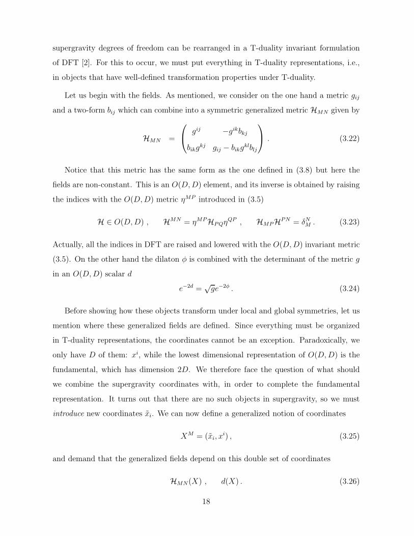
Let us begin with the fields. As mentioned, we consider on the one hand a metric gij

and a two-form bij which can combine into a symmetric generalized metric HMN given by

HMN =

gij −gikbkjbikg

kj gij − bikgklblj

. (3.22)

Notice that this metric has the same form as the one defined in (3.8) but here the

fields are non-constant. This is an O(D,D) element, and its inverse is obtained by raising

the indices with the O(D,D) metric ηMP introduced in (3.5)

H ∈ O(D,D) , HMN = ηMPHPQηQP , HMPHPN = δNM . (3.23)

Actually, all the indices in DFT are raised and lowered with the O(D,D) invariant metric

(3.5). On the other hand the dilaton φ is combined with the determinant of the metric g

in an O(D,D) scalar d

e−2d =√ge−2φ . (3.24)

Before showing how these objects transform under local and global symmetries, let us

mention where these generalized fields are defined. Since everything must be organized

in T-duality representations, the coordinates cannot be an exception. Paradoxically, we

only have D of them: xi, while the lowest dimensional representation of O(D,D) is the

fundamental, which has dimension 2D. We therefore face the question of what should

we combine the supergravity coordinates with, in order to complete the fundamental

representation. It turns out that there are no such objects in supergravity, so we must

introduce new coordinates xi. We can now define a generalized notion of coordinates

XM = (xi, xi) , (3.25)

and demand that the generalized fields depend on this double set of coordinates

HMN(X) , d(X) . (3.26)

18

From the point of view of compactifications on tori, these coordinates correspond to the

Fourier duals to the generalized momenta PM (3.6). However, here we will consider more

generally a background independent formulation [16] in which the generalized metric [17]

can be defined on more general backgrounds.

It is important to recall that here the coordinates can either parameterize compact or

non-compact directions indistinctively. Even if non-compact, one can still formulate a full

O(D,D) covariant theory. In this case, the duals to the non-compact directions are just

ineffective, and one can simply assume that nothing depends on them. This will become

clear later, when we consider DFT in the context of four-dimensional effective theories.

For the moment, this distinction is irrelevant.

Being in the fundamental representation, the coordinates rotate under O(D,D) as

follows

XM → hMN XN , h ∈ O(D,D) , (3.27)

so they mix under these global transformations. Given that xi and xi are related by

T-duality, the later are usually referred to as dual coordinates. Under O(D,D) transfor-

mations, the fields change as follows

HMN(X)→ hMP hN

Q HPQ(h X) , d(X)→ d(h X) . (3.28)

In the particular case in which h corresponds to T-dualities (3.10) in isometric directions

(i.e. in directions in which the fields have no coordinate dependence), these transforma-

tions reproduce the Buscher rules (3.11) and (3.13) for gij, bij and φ. It can be shown that

the different components of (3.28) are equivalent to (3.11), which were derived assuming

T-duality is performed along an isometry. More generally, the transformation rules (3.28)

admit the possibility of performing T-duality in non-isometric directions [14], the reason

being that DFT is defined on a double space, so contrary to what happens in supergrav-

ity, if a T-duality hits a non-isometric direction the result is simply that the resulting

configuration will depend on the T-dual coordinate.

The reader might be quite confused at this point, wondering what these dual coordi-

nates correspond to in the supergravity picture. Well, they simply have no meaning from

19

a supergravity point of view. Then, there must be some mechanism to constrain the co-

ordinate dependence, and moreover since we want a T-duality invariant formulation, such

constraint must be duality invariant. The constraint in question goes under many names

in the literature, the most common ones being strong constraint or section condition. This

restriction consists of a differential equation

ηMN∂M∂N (. . . ) = 0 (3.29)

where ηMN is the O(D,D) invariant metric introduced in (3.5). For later convenience we

recast it as

Y MPN

Q ∂M∂N (. . . ) = 0 , (3.30)

where we have introduced the tensor

Y MPN

Q = ηMNηPQ (3.31)

following the notation in [45], which is very useful to explore generalizations of DFT to

more general U-duality groups, as we will see in Section 6. The dots in (3.30) represent

any field or gauge parameter, and also products of them. Notice that since the tensor Y is

an O(D,D) invariant, so is the constraint. This means that if a given configuration solves

the strong constraint, any T-duality transformation of it will also do. When written in

components, the constraint takes the form

∂i∂i(. . . ) = 0 , (3.32)

so a possible solution is ∂i(. . . ) = 0, or any O(D,D) rotation of this. Actually, it can

be proven that this is the only solution. Therefore, even if formally in this formulation

the fields depend on the double set of coordinates, when the strong constraint is imposed

the only possible configurations allowed by it depend on a D-dimensional section of the

space. When this section corresponds to the xi coordinates of supergravity (i.e., when all

fields and gauge parameters are annihilated by ∂i), we will say that the strong constraint

is solved in the supergravity frame.

When DFT is evaluated on tori, a weaker version of the strong constraint can be

related to the LMC (3.9). In this case, the generalized fields must be expanded in the

20

modes of the double torus exp(iXMPM), such that when the derivatives hit the mode

expansion, the LMC contraction PMPM makes its appearance. Here we will pursue

background independence, and moreover we will later deal with twisted double-tori only

up to the zero mode, so the level matching condition should not be identified with the

strong constraint (or any weaker version) in this review. We will be more specific on this

point in Section 5.

Throughout this review we will not necessarily impose the strong constraint, and in

many occasions we will explicitly write the terms that would vanish when it is imposed.

The reader can choose whether she wants to impose it or not. Only when we intend to

compare with supergravity in D dimensions we will explicitly impose the strong constraint

and choose the supergravity frame (in these cases we will mention this explicitly). The

relevance of dealing with configurations that violate the strong constraint will become

apparent when we get to the point of analyzing dimensional reductions of DFT, and

the risks of going beyond supergravity will be properly explained and emphasized. Let

us emphasize that DFT is a restricted theory though, so one cannot just relax it and

consider generic configurations: the consistency constraints of the theory are imposed by

demanding closure of the gauge transformations, as we will discuss later. These closure

constraints are solved in particular by the solutions to the strong constraint, but other

solutions exist, and then it is convenient to stay as general as possible.

3.4 Generalized Lie derivative

We have seen that the D-dimensional metric and two-form field transform under diffeo-

morphisms (3.14) and that the two-form also enjoys a gauge symmetry (3.16). These

fields have been unified into a single object called generalized metric (3.22), and then

one wonders whether there are generalized diffeomorphisms unifying the usual diffeomor-

phisms (3.14) and gauge transformations (3.16). Since the former are parameterized by

a D-dimensional vector, and the latter by a D-dimensional one-form, one can think of

considering a generalized gauge parameter

ξM = (λi, λi) . (3.33)

21

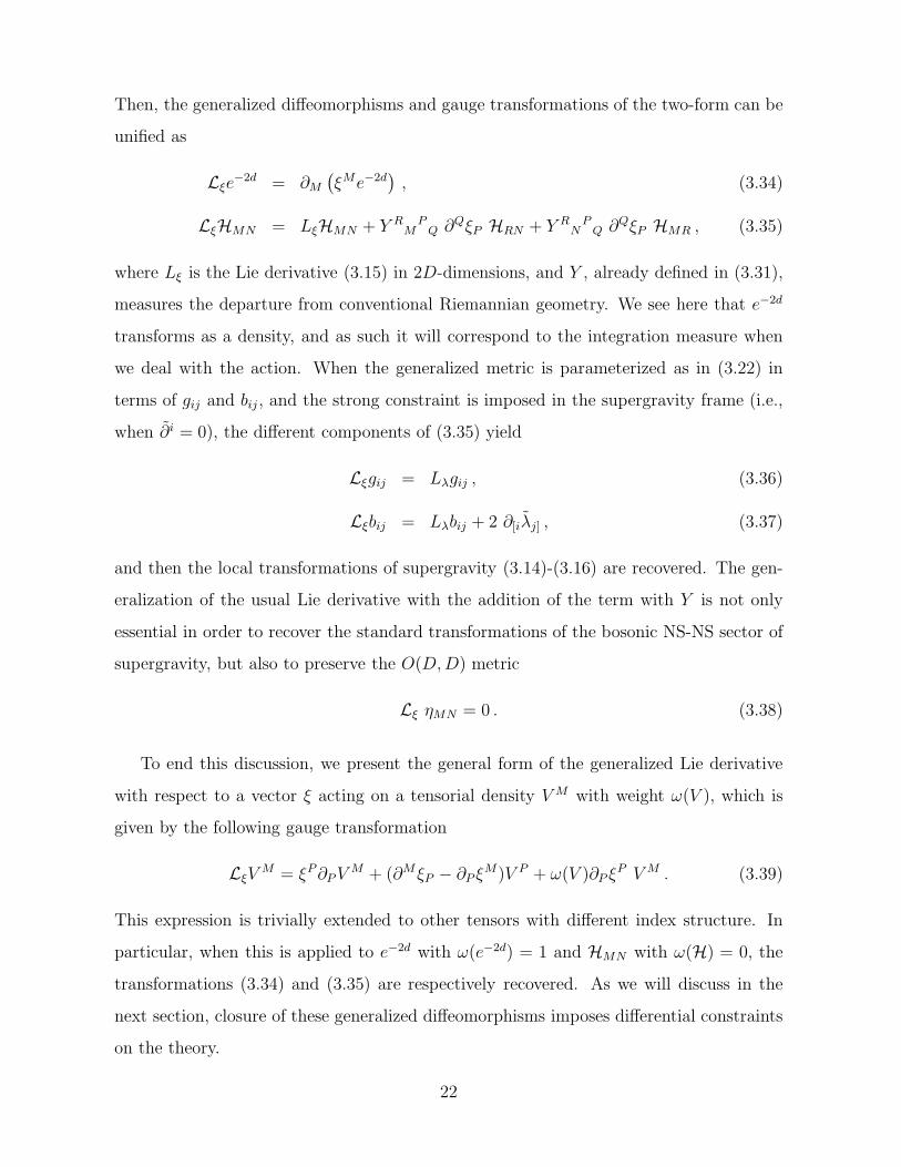
Then, the generalized diffeomorphisms and gauge transformations of the two-form can be

unified as

Lξe−2d = ∂M

(ξMe−2d

), (3.34)

LξHMN = LξHMN + Y RM

PQ ∂QξP HRN + Y R

NPQ ∂QξP HMR , (3.35)

where Lξ is the Lie derivative (3.15) in 2D-dimensions, and Y , already defined in (3.31),

measures the departure from conventional Riemannian geometry. We see here that e−2d

transforms as a density, and as such it will correspond to the integration measure when

we deal with the action. When the generalized metric is parameterized as in (3.22) in

terms of gij and bij , and the strong constraint is imposed in the supergravity frame (i.e.,

when ∂i = 0), the different components of (3.35) yield

Lξgij = Lλgij , (3.36)

Lξbij = Lλbij + 2 ∂[iλj] , (3.37)

and then the local transformations of supergravity (3.14)-(3.16) are recovered. The gen-

eralization of the usual Lie derivative with the addition of the term with Y is not only

essential in order to recover the standard transformations of the bosonic NS-NS sector of

supergravity, but also to preserve the O(D,D) metric

Lξ ηMN = 0 . (3.38)

To end this discussion, we present the general form of the generalized Lie derivative

with respect to a vector ξ acting on a tensorial density V M with weight ω(V ), which is

given by the following gauge transformation

LξVM = ξP∂PV

M + (∂MξP − ∂P ξM)V P + ω(V )∂P ξ

P V M . (3.39)

This expression is trivially extended to other tensors with different index structure. In

particular, when this is applied to e−2d with ω(e−2d) = 1 and HMN with ω(H) = 0, the

transformations (3.34) and (3.35) are respectively recovered. As we will discuss in the

next section, closure of these generalized diffeomorphisms imposes differential constraints

on the theory.

22

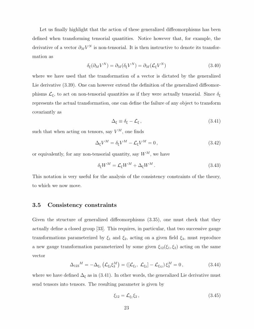
Let us finally highlight that the action of these generalized diffeomorphisms has been

defined when transforming tensorial quantities. Notice however that, for example, the

derivative of a vector ∂MV N is non-tensorial. It is then instructive to denote its transfor-

mation as

δξ(∂MV N ) = ∂M(δξVN) = ∂M (LξV

N ) (3.40)

where we have used that the transformation of a vector is dictated by the generalized

Lie derivative (3.39). One can however extend the definition of the generalized diffeomor-

phisms Lξ, to act on non-tensorial quantities as if they were actually tensorial. Since δξ

represents the actual transformation, one can define the failure of any object to transform

covariantly as

∆ξ ≡ δξ −Lξ , (3.41)

such that when acting on tensors, say V M , one finds

∆ξVM = δξV

M −LξVM = 0 , (3.42)

or equivalently, for any non-tensorial quantity, say WM , we have

δξWM = LξW

M +∆ξWM . (3.43)

This notation is very useful for the analysis of the consistency constraints of the theory,

to which we now move.

3.5 Consistency constraints

Given the structure of generalized diffeomorphisms (3.35), one must check that they

actually define a closed group [33]. This requires, in particular, that two successive gauge

transformations parameterized by ξ1 and ξ2, acting on a given field ξ3, must reproduce

a new gauge transformation parameterized by some given ξ12(ξ1, ξ2) acting on the same

vector

∆123M = −∆ξ1

(Lξ2ξ

M3

)= ([Lξ1, Lξ2 ]− Lξ12) ξ

M3 = 0 , (3.44)

where we have defined ∆ξ as in (3.41). In other words, the generalized Lie derivative must

send tensors into tensors. The resulting parameter is given by

ξ12 = Lξ1ξ2 , (3.45)

23

provided the following constraint holds

∆123M = Y P

RQS

(2∂P ξ

R[1 ∂Qξ

M2] ξS3 − ∂P ξ

R1 ξS2 ∂Qξ

M3

)= 0 . (3.46)

This was written here for vectors with vanishing weight, for simplicity. The parameter

ξ12 goes under the name of D-bracket, and its antisymmetric part is named C-bracket

ξM[12] = [[ξ1, ξ2]]M =

1

2(Lξ1ξ

M2 − Lξ2ξ

M1 ) = [ξ1, ξ2]

M + Y MN

PQ ξQ[1∂P ξ

N2] . (3.47)

It corresponds to an extension of the Lie bracket (3.15), since it contains a correction

proportional to the invariant Y , which in turn corrects the Lie derivative. Respectively,

the D and C-bracket reduce to the Dorfman and Courant brackets [84] when the strong

constraint is imposed in the supergravity frame. Under the constraint (3.46), the following

relation holds

[Lξ1, Lξ2 ] = L[[ξ1, ξ2]] . (3.48)

Notice also that symmetrizing (3.44), we find the so-called Leibniz rule (which arises here

as a constraint)

L((ξ1, ξ2)) = 0 , ((ξ1, ξ2)) = ξ(12) . (3.49)

The D-bracket, which satisfies the Jacobi identity, then contains a symmetric piece that

must generate trivial gauge transformations. This fact is important because on the other

hand, the C-bracket, which is antisymmetric, has a non-vanishing Jacobiator

J(ξ1, ξ2, ξ3) = [[[[ξ1, ξ2]], ξ3]] + cyclic . (3.50)

However, using (3.48) and (3.49), one can rapidly show that [45]

J(ξ1, ξ2, ξ3) =1

3(([[ξ1, ξ2]], ξ3)) + cyclic , (3.51)

and then the Jacobiator generates trivial gauge transformations by virtue of (3.49).

The condition (3.44) poses severe consistency constraints on the generalized diffeomor-

phisms (i.e. their possible generalized gauge parameters). Therefore, DFT is a constrained

or restricted theory. The generalized gauge parameters cannot be generic, but must be

constrained to solve (3.44). Supergravity is safe from this problem, because the usual

24

D-dimensional diffeomorphisms and two-form gauge transformations do form a group.

It is then to be expected that under the imposition of the strong constraint, (3.44) is

automatically satisfied. This is trivial from (3.46) because all of its terms are of the

form (3.30), but more generally these equations leave room for strong constraint-violating

configurations [66, 67, 34], as we will see later.

3.6 The action

The NS-NS sector of DFT has an action from which one can derive equations of motion.

Before showing its explicit form, let us introduce some objects that will be useful later.

The generalized metric can be decomposed as

HMN = EAM SAB EB

N , (3.52)

with an O(D,D) generalized frame

ηMN = EAM ηAB EB

N , (3.53)

where ηAB raises and lowers flat indices and takes the same form as ηMN (3.5). The

generalized frame EAM transforms as follows under generalized diffeomorphisms

LξEAM = ξP∂PE

AM + (∂MξP − ∂P ξM) EA

P , (3.54)

and can be parameterized in terms of the vielbein of the D-dimensional metric gij =

eaisabebj, where sab = diag(−+ · · ·+) is the D-dimensional Minkowski metric, as

EAM =

ea

i eajbji

0 eai

, SAB =

sab 0

0 sab

. (3.55)

Since the Minkowski metric is invariant under Lorentz transformations O(1, D − 1), the

metric SAB is invariant under double Lorentz transformations

H = O(1, D − 1)× O(1, D− 1) (3.56)

which correspond to the maximal (pseudo-)compact subgroup of G = O(D,D). There-

fore, the generalized metric is invariant under local double Lorentz transformations, and

25

thus it parameterizes the coset G/H . The dimension of the coset is D2, and this allows to

accommodate a symmetric D-dimensional metric gij and an antisymmetric D-dimensional

two-form bij , as we have seen. Technically, the triangular parametrization of the general-

ized frame would break down under a T-duality, and then one has to restore the triangular

gauge through an H-transformation. From the generalized frame EAM and dilaton d one

can build the generalized fluxes

FABC = ECMLEAEB

M = 3Ω[ABC] , (3.57)

FA = −e2dLEAe−2d = ΩB

BA + 2EAM∂Md , (3.58)

out of the following object

ΩABC = EAM∂MEB

NECN = −ΩACB , (3.59)

that will be referred to as the generalized Weitzenbock connection.

Since all these objects are written in planar indices, they are manifestly O(D,D) in-

variant, so any combination of them will also be. The generalized fluxes (3.57)-(3.58)

depend on the fields and are therefore dynamical. Later, when we analyze compacti-

fications of the theory, they will play an important role, for they will be related to the

covariant quantities in the effective action, and will moreover reduce to the usual constant

fluxes, or gaugings in the lower dimensional theory, hence the name generalized fluxes.

The generalized frame and dilaton enter in the action of DFT only through the dy-

namical fluxes (3.57) and (3.58). Indeed, up to total derivatives, the action takes the

form

S =

∫dXe−2d R , (3.60)

with

R = FABC FDEF

[1

4SADηBEηCF − 1

12SADSBESCF − 1

6ηADηBEηCF

]

+ FAFB

[ηAB − SAB

]. (3.61)

In this formulation, it takes the same form as the scalar potential of half-maximal super-

gravity in four dimensions. We will be more specific about this later, but for the readers

26

who are familiar with gauged supergravities, notice that identifying here the dynamical

fluxes with gaugings and the SAB matrix with the moduli scalar matrix, this action re-

sembles the form of the scalar potential of [85]. This frame formulation was introduced

in [1], later related to other formulations in [18], and also discussed in [69].

Written in this form, the O(D,D) invariance is manifest. However, some local sym-

metries are hidden and the invariance of the action must be explicitly verified. Under

generalized diffeomorphisms, the dynamical fluxes transform as

δξFABC = ξD∂DFABC +∆ξABC ,

δξFA = ξD∂DFA +∆ξA , (3.62)

where

∆ξABC = 4ZABCDξD + 3∂Dξ[AΩ

DBC] ,

∆ξA = ZABξB + F B∂BξA − ∂B∂BξA + ΩC

AB∂CξB , (3.63)

and we have defined

ZABCD = ∂[AFBCD] −3

4F[AB

EFCD]E = −34ΩE[ABΩ

ECD] , (3.64)

ZAB = ∂CFCAB + 2∂[AFB] − F CFCAB =(∂M∂ME[A

N)EB]N − 2ΩC

AB∂Cd .

The vanishing of (3.63) follows from the closure conditions (3.44), precisely because the

dynamical fluxes are defined through generalized diffeomorphisms (3.57), (3.58)

∆ξFABC = ∆ξABC = ECM∆ξ(LEAEB

M) = 0 ,

∆ξFA = ∆ξA = −e2d∆ξ(LEAe−2d) = 0 . (3.65)

Therefore, the dynamical fluxes in flat indices transform as scalars under generalized

diffeomorphisms.

Let us now argue that due to the closure constraints (3.65), the action of DFT is

invariant under generalized diffeomorphisms. In fact, since e−2d transforms as a density

(recall (3.34))

δξe−2d = ∂P (ξ

Pe−2d) , (3.66)

27

for the action to be invariant under generalized diffeomorphisms, R must transform as

a scalar. Using the gauge transformation rules for the generalized fluxes (3.62) together

with (3.65) one arrives at the following result

δξR = LξR = ξP∂PR . (3.67)

Combining (3.66) with (3.67), it can be checked that the Lagrangian density e−2d Rtransforms as a total derivative, and then the action (3.60) is invariant.

We have seen that in addition to generalized diffeomorphisms, the theory must be

invariant under local double Lorentz transformations (3.56) parameterized by an infinites-

imal ΛAB. This parameter must be antisymmetric ΛAB = −ΛBA to guarantee the invari-

ance of ηAB and it must also satisfy SACΛCB = ΛACS

CB to guarantee the invariance of

SAB. The frame transforms as

δΛEAM = ΛA

BEBM , (3.68)

and this guarantees that the generalized metric is invariant. The invariance of the action

is, however, less clear, and a short computation shows that

δΛS =

∫dX e−2d ZAC ΛB

C (ηAB − SAB) , (3.69)

with ZAB defined in (3.64). Then, the invariance of the action (3.60) under double Lorentz

transformations (3.68) is also guaranteed from closure, since

ZAB = ∆EAFB = 0 . (3.70)

As happens with all the constraints in DFT, which follow from (3.44), they are solved

by the strong constraint but admit more general solutions (this can be seen especially

in (3.46) where cancelations could occur without demanding each contribution to vanish

independently).

This flux formulation of DFT is a small extension of the generalized metric formulation

introduced in [17]. It incorporates terms that would vanish under the imposition of the

strong constraint in a covariant way. After some algebra, it can be shown that the action

28

(3.60) can be recast in the form

S =

∫dXe−2d

(4HMN∂M∂Nd− ∂M∂NHMN − 4HMN∂Md ∂Nd+ 4∂MHMN ∂Nd

+1

8HMN∂MHKL ∂NHKL −

1

2HMN∂MHKL ∂KHNL +∆(SC)R

),

(3.71)

up to total derivatives. Here, we have separated all terms in (3.60) that vanish under

the imposition of the strong constraint ∆(SC)R, to facilitate the comparison with the

generalized metric formulation [17].

To conclude this section, we recall that in order to recover the supergravity action

(3.17), the strong constraint must be imposed in the supergravity frame. Then, when

∂i = 0 is imposed on (3.71), and the generalized metric is parameterized in terms of the

D-dimensional metric and two-form as in (3.22), the DFT action (3.71) reproduces (3.17)

exactly.

3.7 Equations of motion

The equations of motion in DFT were extensively discussed in [32] for different formula-

tions of the theory. For the flux formulation we have just presented, the variation of the

action with respect to EAM and to d takes the form

δES =

∫dX e−2d GABδEAB , (3.72)

δdS =

∫dX e−2d Gδd , (3.73)

where

δEAB = δEAMEBM = −δEBA , (3.74)

to incorporate the fact that the generalized bein preserves the O(D,D) metric (3.5). It

can easily be checked that the variations of the generalized fluxes are given by

δEFABC = 3(∂[AδEBC] + δE[A

DFBC]D

), (3.75)

δEFA = ∂BδEBA + δEABFB , (3.76)

29

δdFA = 2∂A δd . (3.77)

We then obtain

G[AB] = 2(SD[A − ηD[A)∂B]FD + (FD − ∂D)F D[AB] + F CD[AFCDB] , (3.78)

G = −2R , (3.79)

where

F ABC =3

2FD

BCSAD − 1

2FDEFS

ADSBESCF − F ABC . (3.80)

The equations of motion are then

G[AB] = 0 , G = 0 . (3.81)

Upon decomposing these equations in components, and standing in the supergravity frame

of the strong constraint, one recovers the equations of motion of supergravity (3.19)-(3.21),

provided the generalized frame is parameterized as in (3.55).

For completeness let us also mention that had we varied the action in the generalized

metric formulation (3.71) with respect to the generalized metric (and setting to zero the

strong-constraint-like terms), we would have found [17], [32]

δHS =

∫dXe−2dδHMNKMN , (3.82)

with

KMN =1

8∂MHKL∂NHKL −

1

4(∂L − 2(∂Ld))(HLK∂KHMN) + 2∂M∂Nd (3.83)

−12∂(M |HKL∂LH|N)K +

1

2(∂L − 2(∂Ld))(HKL∂(MHN)K +HK

(M |∂KHL|N)) .

Notice however, that the variations δHMN are not generic, but must be subjected to

constraints inherited from (3.23). This implies that only some projections of KMN give

the equations of motion, through a generalized Ricci flatness equation:

RMN = P(MP PN)

QKPQ = 0 , (3.84)

where we introduced some projectors that will be useful in the following section

PMN =1

2(ηMN −HMN ) , PMN =

1

2(ηMN +HMN) . (3.85)

30

Finally, imposing the strong constraint to (3.81) they can be taken to the form (3.84).

These equations of motion will be revisited in the next section from a geometrical

point of view.

31

4 Double Geometry

We have explored the basics of the bosonic NS-NS sector of DFT, starting from its degrees

of freedom, the double space on which it is defined, its consistency constraints, the action

and equations of motion, etc. In particular, the action was tendentiously written in terms

of a generalized Ricci scalar and the equations of motion were cast in a generalized Ricci

flatness form. But, is there some underlying geometry? Can DFT be formulated in

a more fundamental (generalized) geometrical way? It turns out that there is such a

formulation, but it differs from the Riemannian geometry out of which General Relativity

is constructed. We find it instructive to begin this section with a basic review of the

notions of Riemannian geometry that will then be generalized for DFT.

4.1 Riemannian geometry basics

Even though General Relativity follows from an action of the form

S =

∫dx√g R , (4.1)

where R is the Ricci scalar and g the determinant of the metric, we know that there exists

an underlying geometry out of which this theory can be obtained. The starting point can

be taken to be the Lie derivative (3.15)

LξVi = ξk∂kV

i − ∂kξiV k . (4.2)

The derivative of a vector is non-tensorial under the diffeomorphisms (4.2), so one starts

by introducing a covariant derivative

∇iVj = ∂iV

j + ΓikjV k , (4.3)

defined in terms of a Christoffel connection Γ, whose purpose is to compensate the failure

of the derivative to transform as a tensor. Therefore, the failure to transform as a tensor

under diffeomorphisms parameterized by ξ, denoted by ∆ξ, is given by

∆ξΓijk = ∂i∂jξ

k . (4.4)

32

The torsion can be defined through

TijkξiV j = (L∇

ξ − Lξ)Vk = 2Γ[ij]

kξiV j . (4.5)

The superscript ∇ is just notation to indicate that, in the Lie derivative, the partial

derivatives should be replaced by covariant derivatives. A condition to be satisfied in

Riemannian geometry is covariant constancy of the metric gij. It receives the name of

metric compatibility

∇igjk = ∂igjk − Γijlglk − Γik

lgjl = 0 . (4.6)

This fixes the symmetric part of the connection

Γ(ij)k =

1

2gkl(∂igjl + ∂jgil − ∂lgij)− gm(iTj)l

mglk . (4.7)

When the connection is torsionless

Tijk = 2Γ[ij]

k = 0 , (4.8)

it is named Levi-Civita. Notice that the Levi-Civita connection is symmetric and com-

pletely fixed by metric compatibility (4.7) in terms of the degrees of freedom of General

Relativity, namely the metric gij

Γijk =

1

2gkl(∂igjl + ∂jgil − ∂lgij) . (4.9)

Let us note that the Levi-Civita connection satisfies the partial integration rule in the

presence of the measure√g

∫dx√g U∇iV

i = −∫

dx√g V i∇iU , (4.10)

given that its trace satisfies

Γkik =

1√g∂i√g . (4.11)

In a vielbein formulation, one also introduces a spin connection Wiab so that

∇ieaj = ∂iea

j + Γikjea

k −Wiabeb

j , (4.12)

33

and compatibility with the vielbein: ∇ieaj = 0, relates the Christoffel connection with

the Weitzenbock connection

Ωabc = ea

i ∂iebj ecj , (4.13)

through

Wiab = Ωca

beci + Γijkea

jebk . (4.14)

For future reference, we also introduce the notion of dynamical Scherk-Schwarz flux,

defined by the Lie derivative as

eciLeaebi = fab

c = 2Ω[ab]c . (4.15)

Notice the analogy with the generalized fluxes (3.57) defined in terms of the generalized

Lie derivative (3.39). Then, the projection of the torsionless spin connection to the space

of fluxes (i.e., its antisymmetrization in the first two indices) is proportional to the fluxes,

given that the projection of the Levi-Civita connection to this space vanishes. In fact, it

can be shown that in general

eaiWib

c =1

2

(fab

c + sadscefeb

d + sbdscefea

d). (4.16)

Then, the spin connection is fully expressible in terms of dynamical Scherk-Schwarz fluxes.

Having introduced the connections and their properties, we now turn to curvatures.

The commutator of two covariant derivatives reads

[∇i, ∇j]Vk = Rijl

k V l − Tijl ∇lV

k , (4.17)

with

Rijlk = ∂iΓjl

k − ∂jΓilk + Γim

kΓjlm − Γjm

kΓilm (4.18)

the Riemann tensor, which is covariant under Lie derivatives. It takes the same form

when it is written in terms of the spin connection

Rijab = Rijk

leakebl = ∂iWja

b − ∂jWiab +Wic

bWjac −Wjc

bWiac , (4.19)

and it has the following properties in the absence of torsion

Rijlk = Rijlmgmk = R([ij][lk]) , R[ijl]

k = 0 , (4.20)

34

the latter known as Bianchi Identity (BI). The Riemann tensor is a very powerful object in

the sense that it dictates how tensors are parallel-transported, and for this reason it is also

known as the curvature tensor. Tracing the Riemann tensor, one obtains the (symmetric)

Ricci tensor

Rij = Rikjk = Rji , (4.21)

and tracing further leads to the Ricci scalar

R = gijRij . (4.22)

The later defines the object out of which the action of General Relativity (4.1) is built,

while the vanishing of the former gives the equations of motion

Rij = 0 . (4.23)

This equation is known as Ricci flatness, and the solutions to these equations are said to

be Ricci flat. Note that the Riemann and Ricci tensors and the Ricci scalar are completely

defined for a torsionless and metric compatible connection in terms of the metric.

Before turning to the generalizations of these objects needed for DFT, let us mention

that combining the above results, the action of General Relativity can be written purely

in terms of dynamical Scherk-Schwarz fluxes as

S =1

4

∫dx√g fab

cfdef[4δac δ

dfs

be − 2δbfδecs

ad − sadsbescf

]. (4.24)

This is also analog to the situation in DFT (3.61).

4.2 Generalized connections and torsion

Some of the ingredients discussed in the last subsection, already found their general-

ized analogs in previous sections. For example, the Lie derivative (4.2) has already been

extended to its generalized version in double geometry in (3.39). The Weitzenbock con-

nection (4.13) has also been generalized in (3.59), and out of it, so have the fluxes (3.57)

been extended to (4.15). Moreover, the actions (4.24) and (3.61) were both shown to be

35

expressible in terms of fluxes. So, how far can we go? The aim of this section is to con-

tinue with the comparison, in order to find similarities and differences between the usual

Riemannian geometry and double geometry. This is mostly based on [1, 18, 28, 24, 29].

Having defined a generalized Lie derivative, it is natural to seek a covariant derivative.

We consider one of the form

∇MVAN = ∂MVA

N + ΓMPNVA

P −WMAB VB

N , (4.25)

with trivial extension to tensors with more indices. Here we have introduced a Christoffel

connection Γ and a spin connection W whose transformation properties must compen-

sate the failure of the partial derivative of a tensor to transform covariantly both under

generalized diffeomorphisms and double Lorentz transformations.

We can now demand some properties on the connections, as we did in the Riemannian

geometry construction. Let us analyze the implications of the following conditions:

• Compatibility with the generalized frame

∇MEAN = 0 . (4.26)

As in conventional Riemannian geometry, this simply relates the Christoffel connec-

tion with the spin connection through

WMAB = EC

M ΩCAB + ΓMN

P EAN EB

P , (4.27)

where we have written the Weitzenbock connection defined in (3.59), which is totally

determined by the generalized frame. Then, this condition simply says that if some

components of the spin (Christoffel) connection were determined, the corresponding

components of the Christoffel (spin) connection would also be.

• Compatibility with the O(D,D) invariant metric

∇MηPQ = 2ΓM(PQ) = 0 . (4.28)

This simply states that the Christoffel connection must be antisymmetric in its two

last indices

ΓMNP = −ΓMPN (4.29)

36

Notice that, since we have seen in (3.59) that the Weitzenbock connection satisfies

this property as well, due to (4.27) so does the spin connection

WMAB = −WMBA . (4.30)

• Compatibility with the generalized metric

∇MHPQ = ∂MHPQ + 2ΓMR(PHQ)R = 0 . (4.31)

Its planar variant ∇MSAB = 0 is then automatically guaranteed if compatibility

with the generalized frame (4.26) is imposed.

The implications of the combined O(D,D) and generalized metric compatibilities is

better understood through the introduction of the following two projectors (3.85)

PMN =1

2(ηMN −HMN ) , PMN =

1

2(ηMN +HMN) , (4.32)

which satisfy the properties

PMQPQ

N = PMN , PM

QPQN = PM

N , PMN + PM

N = δMN . (4.33)

Compatibility with both metrics then equals compatibility with these projectors

∇M PNQ = 0 , ∇M PN

Q = 0 , (4.34)

which in turn implies

PNR PS

Q ΓMRS = PR

Q∂M PNR . (4.35)

Then, compatibility with the generalized metric and O(D,D) metric combined im-

ply that only these projections of the connection are determined.

• Partial integration in the presence of the generalized density e−2d (3.66)

∫e−2dU∇MV M = −

∫e−2dV M∇MU ⇒ ΓPM

P = −2∂Md . (4.36)

Notice that if the generalized frame were compatible, this would imply in turn that

ECN WNA

C = −FA . (4.37)

37

This requirement can also be considered as compatibility with the measure e−2d,

provided a trace part in the covariant derivative is added when acting on tensorial

densities.

• Vanishing torsion. The Riemannian definition of torsion (4.5) is tensorial with

respect to the Lie derivative, but not under generalized diffeomorphisms. In order

to define a covariant notion of torsion, one can mimic its definition in terms of the

Lie derivative, and replace it with the covariant derivative [24]

(L∇ξ − Lξ)V

M = TPQMξPV Q , TPQ

M = 2Γ[PQ]M + Y M

QRSΓRP

S . (4.38)

This defines a covariant generalized torsion, which corrects the usual Riemannian

definition through the invariant Y defined in (3.31), which in turn corrects the

Lie derivative. Vanishing generalized torsion has the following consequence on the

Christoffel connection

2Γ[PQ]M + ΓM

PQ = 0 . (4.39)

If this is additionally supplemented with the O(D,D) metric compatibility (4.28),

one gets that the totally antisymmetric part of the Christoffel connection vanishes

Γ[MNP ] = 0 ⇔ 3W[ABC] = FABC , (4.40)

where the implication assumes generalized frame compatibility.

• Connections determined in terms of physical degrees of freedom. Typically, under

the imposition of the above constraints on the connections, only some of their com-

ponents get determined in terms of the physical fields. In [28], the connections were

further demanded to live in the kernel of some projectors, allowing for a full deter-

mination of the connection. The prize to pay is that under these projections the

derivative is “semi-covariant”, i.e. only some projections of it behave covariantly

under transformations.

As we reviewed in the previous section, compatibility with the O(D,D) metric is absent

in Riemannian geometry. There, metric compatibility and vanishing torsion determine

38

the connection completely, and moreover guarantee partial integration in the presence of

the measure√g. Here, the measure contains a dilaton dependent part, and then one has

to demand in addition, compatibility with the generalized dilaton. An agreement between

Riemannian geometry and double geometry is that vanishing (generalized) torsion implies

that the projection of the spin connection to the space of fluxes is proportional to the

fluxes (4.15) and (4.40).

Despite the many coincidences between Riemannian and double geometry, there is a

striking difference. While in the former demanding metric compatibility and vanishing

torsion determines the connection completely, in double geometry these requirements turn

out to leave undetermined components of the connection. Only some projections of the

connections are determined, such as the trace (4.37) and its full antisymmetrization (4.40),

among others.

To highlight the differences and similarities between Riemannian and double geometry,

we list in Table (1) some of the quantities appearing in both frameworks.

4.3 Generalized curvature

In this section we will assume that the generalized Christoffel and spin connections satisfy

all the conditions listed in Table 1. We would now like to seek a generalized curvature.

The first natural guess would be to consider the conventional definition of Riemann tensor

(4.18) and extend it straightforwardly to the double space, namely

RMNPQ = 2∂[MΓN ]P

Q + 2Γ[M |RQΓ|N ]P

R . (4.41)

However, this does not work because this expression is non-covariant under generalized

diffeomorphisms

∆ξRMNPQ = 2∆ξΓ[MN ]

RΓRPQ + strong constraint . (4.42)

In Riemannian geometry, this would be proportional to the failure of the torsion to be

covariant, which is zero. Here however Γ[MN ]P is not the torsion, because as we have seen,

it is non-covariant. This in turn translates into the non-covariance of the Riemann tensor.

39

Riemannian geometry Double geometry

Frame compatibility W = Ω+ Γ W = Ω + Γ

O(D,D) compatibility −−−−−−− ΓMNP = −ΓMPN

WMAB = −WMBA

Metric compatibility ∂igjk = 2Γi(jlgk)l ∂MHPQ = 2ΓM(P

NHQ)N

Vanishing torsion Γ[ij]k = 0 Γ[MNP ] = 0

W[ab]c = 2fab

c W[ABC] = 3FABC

Measure compatibility Γkik = 1√

g∂i√g ΓPM

P = e2d∂Me−2d

Wbab = fba

b WBAB = −FA

Determined part Totally fixed Only some

Γijk = 1

2gkl(∂igjl + ∂jgil − ∂lgij) projections

Covariance failure ∆ξΓijk = ∂i∂jξ

k ∆ξΓMNP = 2∂M∂[NξP ]

+ ΩRNPΩRMSξ

S

Table 1: A list of conditions is given for objects in Riemannian and double geometry, with

their corresponding implications on the connections. Every line assumes that the previous

ones hold.

As explained above, one has to resort to a generalized version of torsion (4.38)

TPQM = 2Γ[PQ]

M + Y MQRSΓRP

S = 0 . (4.43)

In addition, even if the first term in (4.42) were zero, we would have to deal with the

other terms taking the form of the strong constraint if we were not imposing it from the

beginning. For the moment, let us ignore them, and we will come back to them later.

Notice that vanishing torsion (4.43) implies

∆ξRMNPQ = −∆ξΓRMNΓRPQ + strong constraint , (4.44)

and then it is trivial to check that the following combination

RMNPQ = RMNPQ +RPQMN + ΓRMNΓRPQ + strong constraint (4.45)

40

is tensorial up to terms taking the form of the strong constraint:

∆ξRMNPQ = strong constraint . (4.46)

Taking the strong constraint-like terms into account, the full generalized Riemann

tensor is given by

RMNPQ = RMNPQ +RPQMN +1

2DY R

LSL (ΓRMNΓSPQ − ΩRMNΩSPQ) , (4.47)

and is now covariant up to the consistency constraints of the theory discussed in Section

3.5.

Since the connection has undetermined components, so does this generalized Riemann

tensor. This combination of connections and derivatives does not project the connections

to their determined part, so we are left with an undetermined Riemann tensor. The

projections of the Riemann tensor with the projectors (4.32) turn out to be either van-

ishing or unprojected as well. This situation marks a striking difference with Riemannian

geometry.

We can now wonder whether some traces (and further projections) of this generalized

Riemann tensor lead to sensible quantities, such as some generalized Ricci tensor related to

the equations of motion of DFT (3.81), or some generalized Ricci scalar related to (3.61).

For this to occur, the traces must necessarily project the connections in the Riemann

tensor in such a way that only their determined part survives.

Tracing the generalized Riemann tensor with the projector P (4.32), one can define a

generalized notion of Ricci tensor

RMN = P PQRMPNQ , (4.48)

from which the action of DFT and its equations of motion can be obtained from traces

and projections. Taking another trace one recovers the (already defined) generalized Ricci

scalar

R =1

4PMNRMN (4.49)

that defines the action of DFT (it actually gives this tensor up to terms that constitute

total derivatives when introduced in the action (3.60)). On the other hand, the following

41

projections of this new generalized Ricci tensor contain the information on the equations

of motion (3.81)

G[MN ] = P[MP PN ]

Q RPQ = 0 . (4.50)

It might be quite confusing that the projections of the generalized Ricci tensor yielding

the equations of motion correspond to the vanishing of an antisymmetric tensor. However,

there is a remarkable property of matrices of the form (4.50)

PMRPN

SRRS = 0 ⇒ P[MRPN ]

SRRS = 0 ⇒ PQM P[M

RPN ]SRRS = 0

⇑ m ⇓PQ

M P(MRPN)

SRRS = 0 ⇐ P(MRPN)

SRRS = 0 ⇐ PMRPN

SRRS = 0

. (4.51)

Therefore, the vanishing of the antisymmetric part of PMRPN

SRRS contains the same

information as the vanishing of the symmetric part. Then, one can alternatively define

a symmetric generalized Ricci tensor whose vanishing yields the equations of motion as

well

RMN = P(MRPN)

S RRS = 0 . (4.52)

We summarize some differences between the geometric quantities in Riemannian and

double geometry in Table (2).

Riemannian geometry Double geometry

Torsion Tijk = 2Γ[ij]

k TMNP = 2Γ[MN ]

P + ΓPMN

Riemann tensor Determined Undetermined

Rijlk = 2∂[iΓj]l

k RMNPQ = RMNPQ +RPQMN

+2Γ[i|mkΓ|j]l

m +ΓRMNΓRPQ − ΩRMNΩ

RPQ

Ricci tensor Determined Undetermined

Rij = Rikjk RMN = PP

QRMQNP

EOM Rij = 0 P(MRPN)

S RRS = 0

Ricci Scalar R = gijRij R = 14PMNRMN

Table 2: A list of definitions of curvatures is given for Riemannian and double geometry.

42

An alternative to this approach was considered in [30], where only the Weitzenbock

connection is non-vanishing and the spin connection is set to zero. The Weitzenbock

connection is torsionful, and the torsion coincides with the generalized fluxes (3.57). This

connection is flat, and then the Riemann tensor vanishes, but the dynamics is encoded in

the torsion and one can still build the DFT action and equations of motion from it, by

demanding H-invariance (3.56). Since the connection and torsion are fully determined,

this approach has the advantage of the absence of unphysical degrees of freedom. This

also has a general relativity analog with its corresponding similarities and differences.

4.4 Generalized Bianchi identities

The generalized Riemann tensor satisfies the same symmetry properties as in Riemannian

geometry (4.20)

RMNPQ = R([MN ][PQ]) , (4.53)

plus a set of Generalized BI

R[ABCD] = ZABCD = ∂[AFBCD] −3

4F[AB

EFCD]E , (4.54)

which under the strong constraint in the supergravity frame simply become the BI of

supergravity (3.18) and (4.20), as we will see later. Notice that due to the consistency

constraints (3.44) this vanishes as a in the usual Riemannian case

ZABCD = ∆EAFBCD = EDM∆ALEB

ECM = 0 . (4.55)

BI in DFT were extensively discussed in [29].

43

5 Dimensional reductions

In order to make contact with four-dimensional physics, we have to address the dimen-

sional reduction of DFT. Strictly speaking, we were already assuming that some directions

were compact, but now make the distinction between compact and non-compact direc-

tions precise, and evaluate the dynamics around particular backgrounds. We begin this

section with a brief review of Scherk-Schwarz (SS) compactifications of supergravity [86],

and then extend these ideas to dimensionally reduce DFT to four dimensions, following

[66], [67]. We show that the resulting effective action corresponds to the electric bosonic

sector of half-maximal gauged supergravity [85] containing all duality orbits of electric

fluxes, including the non-geometric ones [68].

5.1 Scherk-Schwarz compactifications

Let us briefly recall how geometric fluxes emerge in SS compactifications of supergravity,

along the lines of [87].

Consider the NS-NS sector of supergravity containing a D-dimensional metric gij =

eiasabej

b, a two-form field bij and a dilaton φ, all depending on D space-time coordinates

xi (we are thinking of D = 10). We will refer to the D−dimensional theory as the

parent theory. When dimensionally reduced to d = D− n dimensions, the resulting lower

dimensional theory will be referred to as the effective theory.

SS reductions can be introduced as the following set of steps to be performed in order

to obtain the effective theory:

• Split coordinates

xi = (xµ, ym) . (5.1)

The coordinates ym, m = 1, . . . , n correspond to the compact space directions, while

xµ, µ = 1, . . . , d are the space-time directions of the effective theory. The former

(latter) are called internal (external).

• Split indices in fields and parameters. The original D-dimensional theory enjoys

44

a set of symmetries and the fields belong to representations of these symmetries.

Upon compactification, the parent symmetry groups will be broken to those of the

effective theory. The fields must then be decomposed into the representations of the

symmetry group in the lower dimensional theory

gij =

gµν + gpqA

pµA

qν Ap

µgpn

gmpApν gmn

, (5.2)

bij =

bµν − 1

2(Ap

µVpν −ApνVpµ) + Ap

µAqνbpq Vnµ − bnpA

pµ

−Vmν + bmpApν bmn

, (5.3)

i.e. into internal, external and mixed components. Notice that here there is an

abuse of notation in that gµν are not the µν components of gij.

Also the parameters of gauge transformations must be split

λi = (ǫµ, Λm) , λi = (ǫµ, Λm) . (5.4)

• Provide a reduction ansatz. The particular dependence of the fields on the external

and internal coordinates is of the form

gµν = gµν(x) , bµν = bµν(x) , (5.5)

Amµ = ua

m(y)Aaµ(x) , Vmµ = ua

m(y)Vaµ(x) ,

gmn = uam(y)u

bn(y)gab(x) , bmn = ua

m(y)ubn(y)bab(x) + vmn(y) ,

and similarly for the dilaton φ = φ(x). The procedure even tells you what form this

ansatz should have. If there is a global symmetry in the theory, such as a shift in

the two-form b→ b+ v, then one simply “gauges” the global symmetry by making

it depend on the internal coordinates v → v(y). The y-dependent elements u(y)

and v(y) are called twists. Once the procedure is over, the dependence on internal

coordinates will disappear, but the information on the twists will remain in the

form of structure-like constants that will parameterize the possible deformations of

the effective action. For this reason, the twist matrices are taken to be constant

in the external directions, because otherwise Lorentz invariance would be explicitly

45

broken by these constants in the effective action. The hatted fields on the other

hand depend only on the external coordinates, and will therefore correspond to the

dynamical degrees of freedom in the effective action. These are a d-dimensional

metric gµν and a two-form bµν , plus 2n vectors (Aaµ, Vaµ), plus n2 + 1 scalars

(gab, bab, φ).

The gauge parameters must be twisted as well

λi =(ǫµ(x), ua

m(y)Λa(x))

, λi =(ǫµ(x), um

a(y)Λa(x)). (5.6)

• Identify residual gauge transformations. The gauge transformations of the parent

supergravity theory are given by Lie derivatives (3.14)

LλVi = λj∂jV

i − V j∂jλi , (5.7)

plus gauge transformations of the two-form (3.16). Plugging the fields and gauge

parameters with the SS form into these, one obtains the resulting gauge transfor-

mations of the effective theory. For example, taking V i = (vµ(x), uam(y)va(x)), one

gets

LλVµ = ǫν∂ν v

µ − vν∂ν ǫµ ≡ Lǫv

µ , (5.8)

and then the d-dimensional Lie derivative of the effective action is obtained. Simi-

larly,

LλVm = ua

m LλVa , (5.9)

where the resulting transformation is gauged

LλVa = LλV

a + fbcaΛbvc , (5.10)

since it receives the contribution from the following combination of twist matrices

fabc = ua

m ∂mubn uc

n − ubm ∂mua

n ucn , (5.11)

which takes the same form as the SS flux (4.15). Even if these objects are defined

in terms of the twist uam, which is y-dependent, given that they appear in the

residual transformations and we look for a y-independent theory, one must impose

46

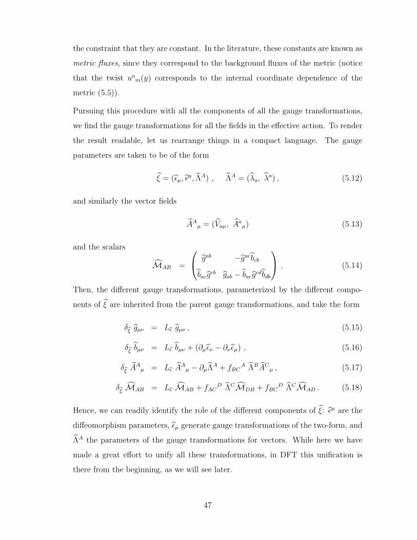
the constraint that they are constant. In the literature, these constants are known as

metric fluxes, since they correspond to the background fluxes of the metric (notice

that the twist uam(y) corresponds to the internal coordinate dependence of the

metric (5.5)).

Pursuing this procedure with all the components of all the gauge transformations,

we find the gauge transformations for all the fields in the effective action. To render

the result readable, let us rearrange things in a compact language. The gauge

parameters are taken to be of the form

ξ = (ǫµ, ǫµ, ΛA) , ΛA = (λa, λa) , (5.12)

and similarly the vector fields

AAµ = (Vaµ, Aa

µ) (5.13)

and the scalars

MAB =

gab −gacbcbbacg

cb gab − bacgcdbdb

. (5.14)

Then, the different gauge transformations, parameterized by the different compo-

nents of ξ are inherited from the parent gauge transformations, and take the form

δξ gµν = Lǫ gµν , (5.15)

δξ bµν = Lǫ bµν + (∂µǫν − ∂ν ǫµ) , (5.16)

δξ AAµ = Lǫ A

Aµ − ∂µΛ

A + fBCA ΛBAC

µ , (5.17)

δξ MAB = Lǫ MAB + fACD ΛCMDB + fBC

D ΛCMAD . (5.18)

Hence, we can readily identify the role of the different components of ξ: ǫµ are the

diffeomorphism parameters, ǫµ generate gauge transformations of the two-form, and

ΛA the parameters of the gauge transformations for vectors. While here we have

made a great effort to unify all these transformations, in DFT this unification is

there from the beginning, as we will see later.

47

Here, we have introduced the “gaugings” or “fluxes” fABC , which have the following

non-vanishing components

fabc = 3(∂[avbc] + f[abdvc]d) ,

fabc = ua

m ∂mubn uc

n − ubm ∂mua

n ucn , (5.19)

while the rest of them vanish

fabc = 0 , fabc = 0 . (5.20)

This compact way of writing the results assumes that indices are raised and lowered

with an O(n, n) metric

ηAB =

0 δab

δab 0

. (5.21)

When written in the form fABC = fABDηDC they are totally antisymmetric fABC =

f[ABC].

• Obtain the d-dimensional effective action. When the SS ansatz is plugged in the

supergravity action, the result is

S =

∫dx√

ge−2φ

(R + 4 ∂µφ∂µφ−

1

4MABFAµνFB

µν (5.22)

− 1

12GµνρGµνρ +

1

8DµMABD

µMAB + V

).

Here R is the d-dimensional Ricci scalar, and we have defined the field strengths as

FAµν = ∂µA

Aν − ∂νA

Aµ − fBC

AABµ AC

ν ,

Gµρλ = 3∂[µbρλ] − fABCAAµA

BρA

Cλ + 3∂[µA

AρAλ]A, (5.23)

and a covariant derivative for scalars as

DµMAB = ∂µMAB − fADCAD

µMCB − fBDCAD

µMAC . (5.24)

Also, due to the gaugings, a scalar potential arose

V = − 1

4fDA

C fCBDMAB − 1

12fAC

E fBDFMAB MCD MEF −

1

6fABCf

ABC ,

(5.25)

48

which strongly resembles the form of the DFT action (3.61). Let us mention that we

have actually considered a simplified ansatz. Lorentz invariance is also preserved if a

warp factor is included in the reductions ansatz, which would turn on additional flux

backgrounds of the form fA, in which case the effective action would exactly coincide

with the DFT action.

This concludes the introduction to the basic notions of SS compactifications of super-

gravity. We should say that there exist different related Scherk-Schwarz compactifications,

and their distinction goes beyond the scope of this review. Also, the consistency of these

reductions is subtle and by no means automatic, and we refer to the literature for detailed

discussions on these points (see for example [8, 88]).

5.2 Geometric fluxes

In the SS reduction defined in (5.5), we restricted to the zero modes and truncated all

the states of the infinite tower of Kaluza-Klein (KK) modes. Had we conserved them, the

effective action would have been more involved and would have had towers of KK degrees

of freedom. Typically, these modes are neglected because their masses scale proportionally

to the order of each mode. If they were kept, other stringy states with comparable masses

should be kept as well, and the effective theory would have to be completed with the

corresponding contributions.

This can be more clearly seen in a toroidal compactification. Indeed, notice that

a compactification on a torus with vanishing background of the two-form corresponds

to taking uam = δam and vab = 0 in the SS procedure. In this case, (5.19) would give

fABC = 0, i.e. we get an ungauged theory. Recalling the mass spectrum of closed strings

on tori (3.1) and the fact that the winding modes decouple in the field theory limit, we

see that the zero mode of such a compactification is massless for the fields considered

in supergravity (with N = N = 1). Had we kept states with p 6= 0, to be consistent

we should have also taken into account other string excitations with comparable masses.

Since all the fluxes vanish in this case, no masses can be generated in the effective theory.

These compactifications on tori with vanishing form fluxes (i.e., configurations with

49

fABC = 0) present many phenomenological problems:

• The scalar potential vanishes, so any configuration of scalars corresponds to a pos-

sible minimum of the theory. The moduli space is then fully degenerate, and all

scalars are massless. This poses a problem because, on the one hand, there are no

massless scalars in nature, and on the other hand, the theory loses all predictability

since one has the freedom to choose any vacuum of the effective theory.

• Since the scalar potential vanishes, there is no way to generate a cosmological con-

stant in the lower-dimensional theory. This is contrary to experimental evidence,

which indicates that our universe has a tiny positive cosmological constant, i.e. it

is a de Sitter (dS) universe.

• The gravitinos of the supersymmetric completion of the theory are massless as well.

If we start with an N = 1 theory in D = 10, we would end with an N = 4 theory

in d = 4. This is too much supersymmetry and we have no possibility to break it.

• Since the fluxes play the role of structure constants, their vanishing implies that

the gauge symmetries are abelian. Then, Standard-Model like interactions are not

possible.

It is then clear that a torus compactification is not interesting from a phenomenological

point of view. The situation changes when the twists uam(y) and vab(y) are such that

fABC 6= 0. We have seen that they allow to turn on metric fluxes fabc (through ua

m) and

two-form fluxes fabc (through vab) in (5.19). The appearance of these fluxes now generates

a scalar potential (5.25) that classically lifts the moduli space. This in turn generates

masses for scalars and gravitinos, renders the gauge symmetries non-abelian and allows

for the possibility of a cosmological constant. However, although the phenomenological

perspectives improved, it turns out that geometric fluxes seem not to be enough for moduli

stabilization and dS vacua, and then one has to go beyond them. There are a number of

no-go theorems and evidence [89] pointing in this direction.

50

In the literature, the two-form and metric fluxes both go under the name of geometric

fluxes, and are denoted

Habc ≡ fabc = 3(∂[avbc] + f[abdvc]d) , (5.26)

ωabc ≡ fab

c = uam ∂mub

n ucn − ub

m ∂muan uc

n

respectively. Since T-dualities exchange metric and two-form components (3.11), they

exchange these fluxes as well

Habch(c)

←→ ωabc . (5.27)

Let us now devote a few lines to give an interpretation of the SS procedure in terms

of a compactification. The SS ansatz (5.5) can be interpreted as follows. The twists

uam(y) correspond to the metric background in the compact space, and gab amount to

perturbations. The full internal metric reads

gmn = uam(y)gab(x)u

bn(y) . (5.28)

When plugging this in the supergravity action, one obtains an effective theory for the

perturbations gmn, that is deformed by parameters that only depend on the background.

Then, freezing the perturbations as

gab(x) = δab ⇒ gmn = uam(y)δabu

bn(y) , (5.29)

gives the background on which one is compactifying, and the effective action dictates

the dynamics of the perturbations around the background. Similarly, the perturbations

of the two-form are given by bab, and freezing them gives the corresponding two-form

background

bab(x) = 0 ⇒ bmn = vmn(y) . (5.30)

The twist matrices uam and vmn can then be interpreted as the backgrounds associated

to the vielbein and the two-form of the compact space. From now on, when referring to

backgrounds we shall assume that the perturbations are frozen.

Let us now explore a very simple setting that gives rise to a flux for the two-form, Habc

(later, we will consider all its T-duals). This is the canonical example in the literature on

51

(non-)geometric fluxes, and it is nicely discussed in [7]. Most of the terminology related

to (non-)geometric fluxes is taken from this example, so we find it instructive to revisit

it here. For simplicity, we consider a three-dimensional internal space, which can be

embedded in the full internal six-dimensional space. Consider a compactification on a

three-torus with a non-trivial two-form

gmn = δmn , b23 = Ny1 ⇔ uma = δam , v23 = Ny1 . (5.31)

Plugging this in (5.26), we obtain

H123 = N , ω123 = ω23

1 = ω312 = 0 , (5.32)

so a compactification on a torus with a non-trivial two-form field turns on a H-flux in the

effective action.

Since this background has isometries in the directions y2, y3, we can perform a T-

duality in one of these directions, lets say h(3), through the Buscher rules (3.11). Then,

we obtain the background

ds2 = gmndymdyn = (dy1)2 + (dy2)2 + (dy3 +Ny1dy2)2 , bmn = 0 . (5.33)

This corresponds to

uam =

1 0 0

0 1 0

0 Ny1 1

, vmn = 0 . (5.34)

Plugging this in (5.26), we find that the fluxes turned on in the effective action are now

H123 = ω231 = ω31

2 = 0 , ω123 = N , (5.35)

in agreement with the T-duality chain (5.27). The background (5.33) is called twisted

torus, and it generates metric fluxes ωabc upon compactifications. In more general back-

grounds, SS compactifications allow to turn on form and metric fluxes simultaneously,

provided the compactification is done on a twisted torus with a non-trivial two-form

background. Examples of different Scherk-Schwarz compactifications in different scenar-

ios, and their relation to gauged supergravity can be found in [90].

52

5.3 Gauged supergravities and duality orbits

The effective action (5.22), obtained by means of a SS compactification, is a particular

gauged supergravity. For a review of gauged supergravity see [8]. These kind of dimen-

sional reductions preserves all the supersymmetry of the parent theory, and are therefore

highly constrained. When the starting point is D = 10 supergravity with N = 1 super-

symmetries (16 supercharges), the d = 4 effective theory preserves all the supercharges

and has therefore N = 4 supersymmetries. This corresponds to half the maximal allowed

supersymmetries, and so they are called half-maximal gauged supergravities. These the-

ories have been widely studied irrespectively of their stringy higher dimensional origin,

and the full set of possible deformations have been classified in [85]. Let us here review

the basics of the bosonic sector of d = 4 half-maximal gauged supergravity, so that we

can then identify particular gaugings as specific reductions in different backgrounds.

The bosonic field content of half-maximal gauged supergravity in four dimensions

consists of a metric gµν , 12 vector fields AAµ and 38 scalars, arranged in two objects:

a complex parameter τ = e−2φ + iB0 and a scalar matrix MAB with 36 independent

components parameterizing the coset O(6, 6)/O(6)×O(6).

There is an additional freedom to couple an arbitrary number N of vector multiplets

but, for simplicity, we will not consider this possibility (otherwise the global symmetry

group would have to be extended to O(D,D + N) [66]). Also, the global symmetry

group contains an SL(2) factor as well, related to S-duality, which mixes electric and

magnetic sectors. This is not captured by DFT (unless the global symmetry group is

further extended to include S-duality) and then one can only obtain the electric sector.

The ungauged theory is invariant under an O(6, 6) global symmetry group, and by

“ungauged” we mean that the gauge group is the Abelian U(1)12. This group can however

be rendered non-Abelian by gauging a subgroup of O(6, 6). Given the O(6, 6) generators

(tα)AB, with α = 1, . . . , 66; A = 1, . . . , 12, there is a powerful object named embedding

tensor ΘAα that dictates the possible gaugings of the theory. The gauge group generators

are given by ΘAα(tα)B

C , so ΘAα establishes how the gauge group is embedded in the global

symmetry group. The 12 ⊗ 66 components of ΘAα are restricted by a linear constraint

53

that leaves only 12 + 220 components, parameterized by

ξA , fABC = f[ABC] , (5.36)

and these are further restricted by quadratic constraints

ξAξA = 0 , (5.37)

ξCfABC = 0 (5.38)

fE[ABfECD] =

1

3f[ABCξD] , (5.39)

necessary for gauge invariance of the embedding tensor (and closure of the algebra). The

O(6, 6) indices are raised and lowered with the invariant metric (5.21).

In four dimensions, two-forms are dual to scalars. Dualizing the scalar B0 → bµν ,

the action of the electric bosonic sector of half-maximal gauged supergravity then takes

the form (5.22) when ξA = 0. We then see that the SS compactification of D = 10

supergravity on a twisted torus with two-form flux leads to a particular half-maximal

gauged supergravity in d = 4. The only possible deformations in that theory are given

by (5.26). From now on we will restrict to the gaugings fABC and set the rest of them to

zero, i.e. ξA = 0, for simplicity.

The global symmetries of the ungauged theory amount to O(6, 6) transformations

AAµ → hB

A ABµ , MAB → hA

C MCD hBD , (5.40)

where the elements h ∈ O(6, 6) were introduced in Section 3.1. When the gaugings are

turned on, the global symmetry group is broken by them. However, O(6, 6) transforma-

tions do not change the physics. In fact, given a configuration of gaugings fABC with

their corresponding action (5.22), any O(6, 6) rotation of them,

fABC → hADhB

EhCFfDEF , (5.41)

would yield a different configuration with a corresponding different action. However,

through a field redefinition of the form (5.40), this action can be taken to the original

form. In other words, we have the relation

S[hA

DhBEhC

FfDEF , AAµ, MAB

]= S

[fABC , hB

AABµ, hA

CMCDhBD], (5.42)

54

and so an O(6, 6) transformation of the gaugings just amounts to a field redefinition.

Then, it corresponds to the same theory. For this reason, it is not convenient to talk

about configurations of gaugings, but rather of orbits of gaugings. An orbit is a set of

configurations related by duality transformations, so that different theories correspond to

different duality orbits of gaugings.

An intriguing feature of gauged supergravities is that they admit more deformations

than those that can be reached by means of geometric compactifications on twisted tori

with two-form flux. In fact, for generic configurations, the embedding tensor has compo-

nents

Qabc = fa

bc , Rabc = fabc , (5.43)

that cannot be turned on through the canonical SS compactification (5.20). Since the

other set of gaugings fabc, fabc were identified with the geometrical fluxes, these are said

to be non-geometric gaugings. Here we have named them Q and R to match the standard

parlance in the literature of flux compactifications. One then wonders to what kind of

backgrounds or compactifications these gaugings would correspond to. As we will see,

T-duality has a very concrete answer to this question.

Before moving to a discussion on non-geometric fluxes, let us briefly review the ar-

guments of [60, 62] to invoke non-geometric fluxes from a string theory perspective. In

[60, 62], all supergravities in D = 10 and 11 dimensions are compactified in a geometric

sense to four dimensions. These higher dimensional supergravities are the low energy limit

of duality related string theories, like for instance Type IIA and Type IIB strings. Each

compactification gives rise to a fluxed effective action containing only geometric fluxes.

When duality transformations are applied at the level of the four dimensional effective

action, one finds that, although the parent theories are connected by dualities, the effective

theories are not [60, 62]. Thus, new non-geometric fluxes have to be invoked so that

the theories match. In this process, gaugings (or fluxes) that look geometric in one

picture (duality frame), are non-geometric in others, and all of them should be included

in string compactifications in order to preserve all the stringy information at the level of the

effective action. Moreover, when all the gaugings are considered together in the effective

55

action, the resulting (super-)potential includes all the possible deformations (gaugings) of

gauged supergravity. All the T-dual deformations are captured by generalized geometric

compactifications of DFT, as we will see.

We have seen in Section 5.2 that starting with a toroidal background with a two-form

flux H123 (5.31), a h(3) T-duality can be performed in the direction y3 leading to a twisted

torus with metric flux ω123 (5.33). The latter still has an isometry in the direction y2, so

nothing prevents us from doing a new T-duality, namely h(2). At the level of fluxes, the

chain would go as

Habch(c)

←→ ωabc h(b)

←→ Qabc , (5.44)

and so a compactification on the resulting background would turn on a Q123 flux in the

effective action. Instead of using the Buscher rules, we find it more instructive to T-

dualize via the construction of a generalized metric. For the twisted torus (5.33) it takes

the form

HMN =

gmn −gmpbpn

bmpgpn gmn − bmpg

pqbqn

=

1 0 0 0 0 00 1 −Ny1 0 0 00 −Ny1 1+(Ny1)2 0 0 00 0 0 1 0 00 0 0 0 1+(Ny1)2 Ny1

0 0 0 0 Ny1 1

.

Now acting on this twisted torus background with a T-duality in the direction y2

HMN → h(2)M

Ph(2)N

QHPQ , h(2) =

( 1 0 0 0 0 00 0 0 0 1 00 0 1 0 0 00 0 0 1 0 00 1 0 0 0 00 0 0 0 0 1

), (5.45)

we get

h(2)M

Ph(2)N

QHPQ =

1 0 0 0 0 00 1+(Ny1)2 0 0 0 Ny1

0 0 1+(Ny1)2 0 −Ny1 00 0 0 1 0 00 0 −Ny1 0 1 00 Ny1 0 0 0 1

, (5.46)

and from here we can obtain the background metric

ds2 = gmndymdyn = (dy1)2 +

1

1 + (Ny1)2[(dy2)2 + (dy3)2] (5.47)

and the two-form

b23 = −Ny1

1 + (Ny1)2(5.48)

associated to the Q123 flux. This background only depends on y1 in the directions or-

thogonal to y1, so this corresponds to a base coordinate. When undergoing a monodromy

56

y1 → y1 + 1, the solution does not come back to itself, but rather to an O(2, 2) ∈ O(3, 3)

rotation of it. Since this duality element mixes the metric and the two-form in a non-

trivial way, it is called a T-fold [14]. From a supergravity point of view, these backgrounds

are globally ill-defined because the T-duality element needed to “glue” the two different

coordinate patches is not an element of the geometric (i.e. diffeos + shifts (3.10)) sub-

group of O(3, 3). This background is then said to correspond to a globally non-geometric

flux Qabc. Notice however that from the double-space point of view there is no such global

issue provided one allows transitions with the full O(3, 3) symmetry group (including

T-dualities (3.10)). In this case, the identifications between the coordinates under mon-

odromies involve the dual ones, and the generalized bein is globally well defined on the

double space.

If we intended to do a further T-duality [60], say in the direction y1,

Habch(c)

←→ ωabc h(b)

←→ Qabc h(a)

←→ Rabc , (5.49)

we would face the problem that we ran out of isometries. Therefore the resulting back-

ground would have to depend on a “dual” coordinate and we would lose any notion of

locality in terms of the usual coordinates on which supergravity is defined. For this rea-

son, the fluxes Rabc are usually named locally non-geometric. Clearly, again, this form of

non-geometry is not a problem in the double space either.

Notice that the chain (5.49) connects different configurations of gaugings via T-duality.

By definition, they all correspond to the same orbit, so the four dimensional theory really

does not distinguish between compactifications on tori with two-form flux, twisted tori

or T-folds, that are connected by T-dualities. In this sense, the orbit itself is basically

geometric: if we were given an action with a single flux, either H , ω, Q or R, we would

always find a geometric uplift and face its corresponding phenomenological problems. A

different situation would be that of an action containing both geometric and non-geometric

fluxes simultaneously turned on. T-duality would exchange geometric with non-geometric

fluxes, and it would never be able to get rid of the non-geometric ones. This kind of

configurations are said to belong to a duality orbit of non-geometric fluxes [68], and they

cannot be reached by means of a standard SS compactification of supergravity. They

57

are actually the most interesting orbits since they circumvent all the no-go theorems

preventing moduli fixing, dS vacua, etc. [89].

As we will see, being T-duality invariant and defined on a double space, DFT is free

from global and local issues. Generalized SS compactifications of DFT will be the topic of

the forthcoming subsections. We will see that DFT provides a beautiful geometric uplift

of all duality orbits, including the non-geometric ones. We anticipate the final picture in

Figure 5.3.

Supergravity D-dimO(D,D)

//❴❴❴❴❴❴❴

Geometric SS

DFT

Generalized SS

Gauged supergravity

d-dim (geometric fluxes) O(n,n)

///o/o/o/o/o/o/o/o/oGauged supergravity

d-dim (all fluxes)

Figure 1: We picture the logic of DFT compactifications [66]. While standard SS re-

ductions from supergravity in D = d + n dimensions (solid line) give rise to gauged

supergravity involving only geometric fluxes in d dimensions, invoking duality arguments

at the level of the effective action one can conjecture the need for dual fluxes [60, 62] to

complete all the deformations of gauged supergravity (waved line). More fundamentally,

DFT is the O(D,D)-covariantization of supergravity (dashed line), and generalized SS

compactifications of DFT give rise to gauged supergravities with all possible deformations

(dotted line).

5.4 Generalized Scherk-Schwarz compactifications

Here we generalize the SS procedure in a duality covariant way by applying it to DFT.

This and the following sections are mostly based on [66, 67, 34]. Let us then follow the

58

steps introduced in Section 5.1, although in a different order for convenience.

• In the double space we have coordinates XM = (xi, xi), so we split them as follows

xi = (xµ, ym) and xi = (xµ, ym). As before, m = 1, . . . , n are indices denoting

internal directions and µ = 1, . . . , d are space-time indices. Then, we have a double

external space and a double internal one with coordinates X = (xµ, xµ) and Y

A =

(ym, ym), respectively.

• Next we propose a reduction ansatz for the fields and gauge parameters in the theory,

inspired in the global symmetries of DFT. For the generalized bein and dilaton we

have

EAM(X) = EA

I(X) UIM(Y) , d(X) = d(X) + λ(Y) , (5.50)

and for the gauge parameters we have

ξM(X) = ξI(X) UIM(Y) . (5.51)

Here M,N = 1, . . . , 2D are curved indices in the parent theory and I, J = 1, . . . , 2D

are curved indices in the effective theory. Again we use the notation that hatted

objects are X-dependent, and all the (double) internal Y-dependence enters through

the twists UIM ∈ O(n, n) and λ.

• We plug this ansatz in the generalized fluxes, and get

FABC = FABC + fIJK EAIEB

JECK , (5.52)

FA = FA + fI EAI , (5.53)

where we have split the coordinate dependence in X-dependent quantities

FABC = 3Ω[ABC] , ΩABC = EAI∂IEB

JECJ , (5.54)

FA = ΩBBA + 2EA

I∂I d , (5.55)

and Y-dependent ones

fIJK = 3Ω[IJK] , ΩIJK = UIM∂MUJ

NUKN , (5.56)

59

fI = ΩJJI + 2UI

M∂Mλ . (5.57)

This splitting is possible provided one imposes the following constraint on the duality

twist UIM

UIM∂M g = ∂I g , ∂MUI

N ∂M g = 0 (5.58)

This restriction on the duality twist, implies that it must be trivial in the X-

directions. There is a very important physical reason for this constraint to hold.

The quantities fIJK and fI are named gaugings, and we take them to be constant

fIJK = constant , fI = constant . (5.59)

This is due to the fact that they appear in the action through the generalized fluxes

FABC and FA, and since we look for a Y-independent effective Lagrangian, they

must be Y-independent because their dependence comes only through the gaugings,

which were requested to be constant. This in turn implies that the internal space

is paralellizable, namely, the twist must be globally defined. The constraint (5.58)

can be recast as

fIJK∂K g = 0 , f I∂I g = 0 . (5.60)

Its effect is to protect Lorentz invariance in the reduced theory. Notice that ∂I g

is only non-vanishing in the external directions, and then if the gaugings had legs

in these directions they would explicitly break Lorentz symmetry. Therefore, fIJK

and fI can only be non-vanishing along the double internal space. For simplicity

here we will only analyze the case fI = 0, since consistency of the theory would

otherwise require a slightly modified reduction ansatz. A discussion on how to turn

the gaugings on in the usual supergravity picture can be found in [91], and in a

duality covariant way in DFT in [67].

• We next plug (5.52) and (5.53) into the action of DFT (3.60) to obtain the effective

theory

SGDFT = v

∫dXe−2d

[−14

(FIK

L + fIKL

)(FJL

K + fJLK

)HIJ (5.61)

60

− 1

12

(FIJ

K + fIJK

)(FLH

G + fLHG

)HILHJHHKG

−16

(FIJK + fIJK

)(F IJK + f IJK

)+

(HIJ − ηIJ

)FIFJ

].

The internal coordinate dependence factorized, and it just amounts to an overall

constant factor

v =

∫dYe−2λ . (5.62)

If the gaugings vanished fIJK = 0, one recovers the usual DFT action (3.60) in

less dimensions. This then corresponds to a gauged DFT (GDFT) [21, 34] (see [71]

for a geometric and supersymmetric treatment of GDFT), which has been obtained

through a generalized SS compactification of a higher dimensional parent DFT.

• The symmetries of the GDFT are inherited from those of the parent DFT. For

instance, the generalized Lie derivative induces the gauge transformations in the

effective action

LξVM = UI

M LξVI , (5.63)

namely

LξVI = LξV

I − f IJK ξ

J V K . (5.64)

The first term is the usual generalized Lie derivative, and the second one amounts

to a deformation due to the gaugings. These induced transformations now close (in

the sense of (3.46)) when the following quadratic constraints are imposed on the

gaugings

fH[IJfKL]H = 0 , (5.65)

and the strong constraint holds in the external space

∂I V ∂IW = 0 (5.66)

for any hatted quantity, such as effective fields or gauged parameters. The action

of GDFT (5.61) is invariant under (5.64) up to these constraints. Moreover, it can

be checked that compactifying the constraints of the parent DFT gives the same

result that one would obtain by directly computing the consistency conditions of the

effective GDFT. These amount to even more relaxed versions of (5.65) and (5.66).

61

5.5 From gauged DFT to gauged supergravity

Now that we have built a covariant formulation of the effective theory, we can choose to

solve the effective strong constraint (5.66) in the usual frame of a gauged supergravity

∂I V ∂IW = 0 → ∂µV = 0, i.e. we solve the strong constraint in the effective action

by demanding that the effective fields and gauged parameters only depend on xµ. Due

to the coordinate splitting X → X,Y a convenient re-parameterization of the effective

generalized metric HIJ is in order. The O(D,D) group is now broken to O(d, d)×O(n, n),

and then it is convenient to rotate the group metric to the form

ηIJ =

δµν

δµν

ηAB

, (5.67)

where ηAB was defined in (5.21). This amounts to a re-parameterization of the generalized

bein

EAI =

eaµ −eaρcρµ −eaρAAρ

0 eaµ 0

0 ΦABA

Bµ ΦA

A

, (5.68)

which is now associated to the following generalized metric

HIJ =

gµν −gµρcρν −gµρAAρ

−gνρcρµ gµν + ACµMCDA

Dν + cρµg

ρσcσν MACACµ + AAρg

ρσcσµ

−gνρABρ MBCACν + ABρg

ρσcσν MAB + AAρgρσABσ

. (5.69)

Here we have introduced the combination cµν = bµν+12AB

µABν . Also, AAµ are the vectors

(5.13) and ΦAA is the scalar bein for the scalar metric MAB defined in (5.14). Notice

that we have run out of indices, so we are denoting with the same letter A the full flat

index, and the internal one, the distinction should be clear from the context. Also due to

the splitting, now the gaugings are only non-vanishing in the internal components

fIJK =

fABC (I, J,K) = (A,B,C)

0 otherwise. (5.70)

Then, plugging (5.68) and (5.70) into (5.54), and taking into account that the indices

are now raised and lowered with (5.67), we can readily identify some of the components

62

of the compactified generalized fluxes with covariant quantities in the effective action

(5.23)-(5.24), namely

Fabc = eaµeb

ν ecρ Gµνρ , (5.71)

FabC = ea

µebνΦC

C FCµν , (5.72)

FaBC = ea

µΦCC DµΦB

C , (5.73)

where

DµΦBC = ∂µΦB

C − fABCAµ

AΦBB (5.74)

is the covariant derivative of the scalar bein. Finally, plugging (5.68) and (5.70) in the

action (5.61) of GDFT, one recovers the effective action of gauged supergravity (5.22).

Therefore, gauged supergravities are particular examples of GDFT.

5.6 Duality orbits of non-geometric fluxes

Even if it looks like the generalized SS procedure discussed in Sections 5.4 and 5.5 leads

to the same action (5.22) obtained from the usual geometric SS compactification of Sec-

tion 5.1, this is not correct. The difference resides in the gaugings. While the geometric

SS reduction only allows to turn on the fluxes (5.19) and the others (5.20) vanish, the

generalized SS reduction of DFT allows, in principle, to turn on all the gaugings simulta-

neously.

We have defined the gaugings or fluxes in (5.56) in terms of a duality valued twist

matrix U(Y) ∈ O(n, n). This generalizes the usual SS gaugings in two ways:

• Global extension. The geometric SS gaugings are generated through uam and vmn

in (5.19), which respectively correspond to the metric and two-form background.

They can both be combined into the O(n, n) duality twist matrix in the form

UAM =

ua

m uanvnm

0 uam

. (5.75)

A T-duality transformation would break the triangular form of this matrix, into

a new element of O(n, n) containing a South-West component. Therefore, the

63

only backgrounds that are allowed in the usual SS compactification of supergrav-

ity are those that come back to themselves under monodromies, up to u and/or

v-transformations only, i.e. the geometric subgroup of the full O(n, n). In a general-

ized SS compactification, we now allow the duality twist to be a generic element of

O(n, n). This includes, in addition to the elements uam and v[mn], a new component

usually dubbed β [mn]

UAM =

ua

m uanvnm

uanβ

nm uam + ua

nβnpvpm

. (5.76)

The effect of this extension is now to allow for backgrounds that come back to

themselves under monodromies, up to a generic O(n, n) transformation. This is

the case of the T-folds discussed before. Then, the generalized SS compactification

allows for new backgrounds that are globally ill defined from the usual (geometric)

supergravity point of view.

• Local extension. The fluxes (5.56) are now not only defined in terms of an extended

duality twist, but also in terms of a generalized derivative with respect to all coor-

dinates. This would allow for more richness in the space of gaugings, if the duality

twist violated the strong constraint. In this case, the dual coordinate dependence

would make no sense from a supergravity point of view, altering the standard notion

of locality.

Let us now show that the quadratic constraints (5.65) are weaker than the strong

constraint. For the duality twist, the strong constraint implies

ΩEABΩECD = 0 . (5.77)

where ΩABC was defined in (5.56). On the other hand, similar to the BI (3.64), one can

show that

∂[AfBCD] −3

4f[AB

EfCD]E = −34ΩE[ABΩ

ECD] . (5.78)

For constant gaugings the first term drops out, and then we see that the quadratic con-

straints correspond to a relaxed version of the strong constraint (5.77), because they only

require the totally antisymmetric part of (5.77) to vanish.

64

This is however not the end of the story. One has to show that there exist solutions to

the quadratic constraints that violate the strong constraint. As we explained, the gauged

supergravities we are dealing with are half-maximal. Half-maximal gauged supergravities

split into two different groups: those that can be obtained by means of a truncation of

a maximal supergravity, and those that cannot (in d = 4 see [92]). The former inherit

the quadratic constraints of the maximal theory, which in the language of the electric

half-maximal gaugings take the form (for simplicity we take λ = 0 in (5.50))

fABCfABC = 3ΩABCΩ

ABC = 0 . (5.79)

Therefore, the genuine half-maximal theories, which violate the above constraint, must be

necessarily generated through a truly doubled duality twist [68]. On the other hand, when

the strong constraint holds, the only reachable theories are those that admit an uplift to

a maximal supergravity. In Figure 2 we have pictured the kind of orbits that one finds

in half-maximal supergravities (the case d = 4 should be analyzed separately due to the

extra SL(2) factor [92]). Let us stress that the notion of non-geometry discussed in [68] is

local, and then a duality orbit of non-geometric fluxes contains all fluxes simultaneously

turned on Habc, ωabc, Qa

bc and Rabc. However, one could also define a notion of globally

non-geometric orbit, which could admit a representative without Rabc-flux.

The idea of combining geometric with non-geometric fluxes simultaneously is usually

considered with some precaution. It is common to find objections against these config-

urations mostly based on scaling arguments. The non-geometric fluxes are sometimes

associated to windings (since they are mostly generated through dual coordinate depen-

dence), while the geometric ones are related to momentum. A quick look at the mass

formula (3.1) shows that, for a given radius R, when momentum (winding) modes are

heavy, the winding (momentum) modes are light. Considering both of them simultane-

ously then leads to unavoidable heavy modes in the spectrum. This enters in conflict with

the fact that one is truncating the heavy mass levels of the string from the beginning.

The conclusion of this argument is that one should then impose the strong constraint, so

as to truncate the heavy part of the spectrum, and this in turn only permits geometric

orbits.

65

A

B

Orbits (1)

Orbits (2)Flux space

Geometric fluxes

Figure 2: We picture the space of gaugings (or fluxes) in half-maximal supergravities

in d = 7, 8 [68]. A point in this diagram corresponds to a given configuration. If two

points lie in the same diagonal line (orbit) they are related by a duality transformation.

Different theories are classified by orbits (lines) rather than configurations (points). The

configuration space splits in a subgroup of geometric (i.e. only involving fluxes like Habc

and ωabc) and non-geometric (involving fluxes Qa

bc and Rabc) configurations. The space of

orbits then splits in two: (1) non-geometric orbits (truly half-maximal) and (2) geometric

orbits (basically maximal) that intersect the geometric space (between A and B).

Notice however that these arguments are purely based on the KK-mode expansions

of fields on tori. The relation between (winding) momentum and (dual) coordinates, is

given by the Fourier transforms of the KK-modes of the torus. Moreover, the mass formula

(3.1) only holds for tori. In this section, we do not consider tori, and moreover, we do not

consider KK excitations. We only consider the zero-modes of the fields on twisted-double-

tori. The only connection between these two situations is when the duality twist is taken

to be constant, in which case we would be dealing with the (massless) zero-modes on a

torus, as discussed in section 5.2. When the twist matrix is non-constant, the effective

theory becomes massive, but these masses are corrections to the massless modes on the

torus through a twist. We are then correcting massless modes, through a procedure that

truncates all the problematic (KK) modes. When dealing with moduli fixing, one has

to make sure that for a given non-geometric orbit, the masses of the scalar fields (which

66

are totally unrelated to (3.1)) in a given vacuum are small compared to the scales of the

modes we are neglecting.

A similar reasoning prevents us from relating the strong constraint (or a weaker version

of it) with the LMC condition (3.9), as we explained in Section 3.3. If we had considered

tori compactifications, and kept the tower of excited states, whenever the derivatives in

strong-constraint like terms acted on the mode expansion they would form contractions

like PMPM related to the LMC. Here, we are considering the zero-modes, for which

PMPM = 0 is trivially satisfied because PM = 0. Then, in SS compactifications in which

the tower of KK modes is truncated, it might not be correct to identify the LMC with

strong-like constraints. Instead, the consistency constraints are given by the quadratic

constraints for gaugings (5.65).

Combining fluxes and their derivatives, it is possible to construct three quantities that

vanish upon imposition of the strong constraint [69]:

∂[AfBCD] −3

4f[AB

EfCD]E = ZABCD , (5.80)

∂EfEAB + 2∂[AfB] − fEfEAB = ZAB , (5.81)

∂EfE −1

2fEfE +

1

12fABCf

ABC = Z . (5.82)

They correspond to duality orbits of generalized BI for all the dual fluxes. The first

two (5.80), (5.81) are related to the constraints of the theory, and are obtained from

compactifications of (3.64). The last one (5.82) was associated to the embedding of the

theory into a maximal theory (5.79).

The fluxes fABC encode the standard T-dual fluxes, as we reviewed. This can be seen

by splitting the indices as

fabc = Habc , fabc = ωbc

a , fabc = Qc

ab , fabc = Rabc . (5.83)

Through T-dualities they are related according to the chain (5.49). Recall that we are

only dealing here with the case fA = 0. Splitting in components equation (5.80), we find

∂[aHbcd] −3

2He[abωcd]

e = Zabcd ,

67

3∂[aωbc]d − ∂dHabc + 3ω[ab

eωc]ed − 3Q[a

deHbc]e = Zabcd ,

2∂[aQb]cd + 2∂[cωab

d] − ωabeQe

cd −HabeRecd + 4Q[a

e[cωb]ed] = Zab

cd , (5.84)

3∂[aQdbc] − ∂dR

abc + 3Qe[abQd

c]e − 3ωde[aRbc]e = Zabc

d ,

∂[aRbcd] − 3

2Re[abQe

cd] = Zabcd .

These reduce to those of [60] for constant fluxes under the strong constraint, and to those

of [93] for non-constant fluxes. Equation (5.82), on the other hand, reads in components

1

6HabcR

abc +1

2ωab

cQcab = Z . (5.85)

This corresponds to an orthogonality-like condition between geometric (Habc, ωabc) and

non-geometric (Qabc, Rabc) fluxes, as expected. And this is the reason why the failure of

this equation to vanish requires non-geometric fluxes. Therefore, (5.85) can be used to

classify duality orbits of non-geometric fluxes.

Using the extended parameterization of the twist matrix (5.76)

UAM =

ua

m uanvnm

uanβ

nm uam + ua

nβnpvpm

, (5.86)

and inserting this in the definition of the fluxes (5.56), (5.70)

fABC = 3 U[A|M ∂MU|B

NUC]N , (5.87)

we find in components

Habc = 3[∇[avbc] − vd[a∇dvbc]

], (5.88)

ωabc = 2Γ[ab]

c + ∇cvab + 2Γmc[avb]m + βcmHmab ,

Qcab = 2Γ[ab]

c + ∂cβab + vcm∂

mβab + 2ωmc[aβb]m −Hmncβ

maβnb ,

Rabc = 3[β [am∇mβ

bc] + ∇[aβbc] + vmn∇nβ [abβc]m + β [amβbn∇c]vmn

]+ βamβbnβclHmnl ,

where we have used the following relations and definitions

uamua

n = δmn , uamub

m = δba , vab = uamub

nvmn , βab = uamu

bnβ

mn ,

68

∂a = uam∂m , ∂a = ua

m∂m ,

∇avbc = ∂avbc − Γabdvdc − Γac

dvbd , ∇avbc = ∂avbc + Γadbvdc + Γad

cvbd ,

∇aβbc = ∂aβ

bc + Γadbβdc + Γad

cβbd , ∇aβbc = ∂aβbc − Γabdβ

dc − Γacdβ

bd ,

and

Γabc = ua

m∂mubnecn , Γab

c = uam∂

mubnuc

n . (5.89)

The expressions (5.88) are very useful to explore the uplifting of fluxes to higher dimen-

sional theories. Notice that while Habc and ωabc can be generated through geometric twists

uam and vmn, the non-geometric fluxes Qa

bc and/or Rabc require β-twists and/or dual co-

ordinate dependence. This also serves to show that the distinction between “globally”

and “locally” non-geometric fluxes is just a terminology inherited from the toy example

discussed before, since Qabc can arise from dual coordinate dependence, and Rabc can arise

from globally non-geometric compactifications with non-trivial β-twist. Setting βij = 0

and ∂i = 0, the expressions (5.88) reduce to (5.26).

69

6 U-duality and extended geometry

The compactification of D = 11 supergravity and M-theory on an n-dimensional torus,

enjoys a U-duality symmetry En(n) (see for example [94, 95, 96]). The idea of extending

the space-time and/or the tangent space so as to accommodate such symmetries was

introduced in [38], [39] and more recently considered in [40, 44, 46]. In this section, we

review some of the approaches to replace the T-duality group by the U-duality group, in

order to incorporate all the extra fields (like R-R in Type II theories or the three-form

of M-theory) in a duality covariant manner, much under the same philosophy as that of

DFT.

6.1 Generalized diffeomorphisms and the section condition

We have seen that the generalized diffeomorphisms of DFT (3.39) discussed in the previous

sections enjoy the following properties:

• They preserve the duality group invariant, in that case the O(D,D) metric ηMN .

• They are defined in terms of an invariant Y -tensor related to the definition of the

strong constraint.

• They reproduce the gauge transformations of the D-dimensional metric and two-

form, upon application of the strong constraint.

• When “twisted”, they give rise to fluxes or gaugings in the representations allowed

by supersymmetry.

• Their closure imposes a set of constraints that, on the one hand are solved by

the strong constraint, and on the other, reproduce the quadratic constraints of the

supergravity gaugings upon “twisting”.

Clearly, the inclusion of other fields, like R-R sector in Type II string theory or the more

general three-form of M-theory, requires an enlargement and further generalization of the

70

already generalized Lie derivative, to be compatible now with U-duality. All the trans-

formation properties of gravitational and tensorial degrees of freedom, which mix under

U-duality, must now be accommodated (and unified) in a new generalized Lie derivative.

We will see that such a generalized transformation enjoys the U-duality extension of the

properties listed above.

This generalization is a little more involved since the U-duality group jumps with

dimension. For the n internal dimensions of M-theory, it corresponds to exceptional groups

En(n), and in n > 8 one encounters the complication of infinite-dimensional Kac-Moody

type algebras. Given the disconnected structure of the groups for different dimensions, it

is convenient to work case by case. As in DFT, where the space is doubled to account for

the winding degrees of freedom of the string, here the space is further enlarged to account

for the wrapping states of M-branes. The internal space is then replaced by an extended

mega-space with extended dimensions, and here for simplicity we neglect the external

space-time. Relevant representations for the different U-duality groups are given in Table

3. The mega-space associated to each of them is dim(R1)-dimensional.

R1 R2

E4(4) = SL(5) 10 5

E5(5) = SO(5, 5) 16 10

E6(6) 27 27

E7(7) 56 133

Table 3: Some relevant representations of U-duality groups [45].

The generalized diffeomorphisms [47, 44] formally preserve the structure of those an-

alyzed before for DFT (we are using the notation of [45])

LξVM = LξV

M + Y MN

PQ ∂P ξ

Q V N , (6.1)

where Y is a U-duality invariant tensor “measuring” the departure from the usual Lie

derivative. It can be generically decomposed as

Y MN

PQ = δMQ δPN − αP(adj)

MN

PQ + βδMN δPQ , (6.2)

71

where P(adj) is a projector to the adjoint representation of the U-duality group, α is a

group-theoretical quantity that depends on the dimension, and β is a weight for tensorial

densities that also depends on the group. Indices M,N are in the R1 reps of Table 3,

and P(adj) corresponds to the adjoint projection contained in the tensor product R1⊗R1.

It can be checked that these generalized Lie derivatives preserve the invariants of each

group. The appearance of the last β-term is due to the fact that in the U-duality case

one usually considers En(n) × R+ tensorial densities rather than just tensors (we will be

more specific later).

Before showing the general results, to warm up let us first see how the DFT O(n, n)

case fits in this language. The projector to the adjoint representation is given by

O(n, n) : P(adj)M

NPQ =

1

2(δMQ δPN − ηMPηNQ) , (6.3)

and then, introducing this in (6.2) and comparing with (3.31), we find that the correct

value of the proportionality constants is given by (α, β) = (2, 0) for un-weighted tensors.

More generally, the expression for Y in the different duality groups is given in Table 4.

Y MQN

P α β

O(n, n) ηMNηPQ 2 0

E4(4) = SL(5) ǫiMN ǫiPQ 3 15

E5(5) = SO(5, 5) 12(γi)MN(γi)PQ 4 1

4

E6(6) 10dMNRdPQR 6 13

E7(7) 12KMNPQ + δ

(MP δ

N)Q + 1

2ǫMN ǫPQ 12 1

2

Table 4: Invariant Y -tensor and proportionality constants for different dimensions. Here

ηMN is the O(n, n) invariant metric, ǫiMN is the SL(5) alternating tensor, (γi)MN are

16 × 16 MW representation of the SO(5, 5) Clifford algebra, dMNR and KMNPQ are the

symmetric invariant tensors of E6(6) and E7(7) respectively, and ǫMN is the symplectic

invariant in E7(7). These results were taken from [45], we refer to that paper for more

details.

72

In the U-duality case, there is also an analogue of the strong constraint, also known

as section condition [47, 44]

P(R2)MNPQ∂P∂Q(. . . ) = 0 , (6.4)

which again acts on any product of fields and gauge parameters. Generically, any so-

lution to this condition picks out an n-dimensional subspace of the mega-space, which

can be associated to the physical space in M-theory compactifications. Again, when an-

alyzing closure of these generalized diffeomorphisms, one finds that closure is achieved

automatically when restricted to configurations satisfying the section condition.

Analogously to the DFT case, when a duality twist reduction of these generalized Lie

derivatives is performed, they induce an effective gauge transformation giving rise to the

embedding tensor components of the different maximal gauged supergravities for different

dimensions. The analogies don’t stop here, since it is also possible to construct an ex-

tended geometrical formalism, introducing generalized connections, torsion and covariant

Ricci-like tensors for these generalized transformations. Lets now review how this works,

specializing to the E7(7) case for a detailed exposition.

The cases n ≤ 7 were studied in [44] and [45]. The cases n ≤ 2 just reduce to ordinary

Riemannian geometry. The case n = 4 was studied in [53] in the context of gauged

supergravities, and a geometry for it was considered in [49]. The cases n = 5 and 6 were

related to SS compactifications in [54], and n = 7 in [55], where an extended geometry

was also formulated. A unified geometric description for n ≤ 7 was considered in [50].

The case n = 8 was explored in [51], and for n > 8 the groups are much more involved.

An ambitious programme intended to encompass all formulations under E11 can be found

in [41].

6.2 The E7(7) case and maximal gauged supergravity

E7(7) is the U-duality group of gauged maximal supergravity in four dimensions [97], the

ungauged theory being obtained through compactifications of M-theory on a seven-torus

[98]. The idea here is to replace the internal seven-space by a 56-dimensional mega-space,

73

and accommodate the internal degrees of freedom in a generalized metric HMN defined on

the mega-space. This idea was first considered in [63], and here we will present the results

of [55]. Since we are ignoring the four-dimensional space time, the generalized metric

should be identified with the scalar degrees of freedom of the gauged supergravity. The

generalized metric transforms covariantly under G = E7(7) × R+, and is invariant under

the maximal compact subgroup H = SU(8). It can be written in terms of a generalized

bein EAM taking values in the quotient G/H

EAM = e−∆EA

M , (6.5)

where we have separated a conformal factor ∆ corresponding to the R+ components.

Here the flat indices A, B, . . . take values in H and the curved ones M,N, . . . in G.

Then, EAM lives in the quotient E7(7)/SU(8), and the tilde refers to the E7(7) part of G

only. G has a (weighted) symplectic invariant ωMN that raises and lowers indices, and

a quartic invariant KMNPQ which is totally symmetric. The fundamental representation

of E7(7) is 56 and the adjoint is 133. Given a tensorial density V M , the generalized Lie

derivative (or equivalently the exceptional Dorfman bracket) reads

LξVM = ξP∂PV

M − 12P(adj)M

NPQ ∂P ξ

Q V N − 1

2∂P ξ

P V M . (6.6)

Here P(adj)((MN)(PQ)) is the projector to the adjoint representation, defined in terms of the

E7(7) invariants

P(adj)MNPQ = (tα)NM (tα)PQ =1

12ωM(PωQ)N +KMNPQ . (6.7)

As we did before in the DFT case, here we can compute the closure of these transfor-

mations

∆123M = −∆ξ1Lξ2ξ

M3 = ([Lξ1 , Lξ2 ]−LLξ1

ξ2)ξM3 = 0 , (6.8)

and get

∆[12]3M = Y Q

LOI ∂Oξ

I[2 ξL1] ∂Qξ

M3 + AM

NJLY

QJOI ∂Qξ

I[2 ∂Oξ

L1] ξ

N3

+ QMN

QOLI ∂Q∂Oξ

I[2 ξL1] ξ

N3 = 0 ,

∆(12)3M = −Y Q

LOI ∂Qξ

I(1 ξL2) ∂Oξ

M3 + QM

NQO

LI∂Q(ξL(1 ∂Oξ

I2)) ξ

N3

74

+1

4ωLIω

QO ∂QξL1 ∂Oξ

I2 ξM3 = 0 , (6.9)

where we have defined

QMN

QOLI = Y Q

JO(LA

JI)

MN +

1

2ωILY

QMON −

1

2Y Q

LOIδ

MN . (6.10)

Notice that all derivatives are contracted as

Y MPN

Q∂M∂N =

(1

2ωMNωPQ − 12P(adj)PQ

MN

)∂M∂N . (6.11)

As we mentioned in the previous section, when the so-called section condition (6.4)

P(adj)PQMN∂M∂N(. . . ) = 0 (6.12)

is imposed, the closure condition ∆123M = 0 is automatically satisfied. In fact, it can

be seen that any solution to this condition selects a seven-dimensional subspace of the

full 56-dimensional mega-space, permitting to make contact with the physical internal

compact directions. When (6.12) holds, it can also be proven that ωMN∂M∂N(. . . ) = 0,

and therefore also Y MPN

Q∂M∂N (. . . ) = 0, in analogy with DFT (3.30).

Following the DFT logic (3.57), we can now define a dynamical flux

LEAEB = FAB

CEC , (6.13)

with

FABC = ΩAB

C − 12P(adj)CBDEΩDA

E +1

2ΩDA

DδCB , (6.14)

where

ΩABC = EA

M∂MEBN(E−1)N

C , (6.15)

is the G-generalized Weitzenbock connection. Rotating these expressions with the bein

we can define the fluxes with curved indices

FMNP = ΩMN

P − 12P(adj)PN

RSΩRM

S +1

2ΩRM

RδPN , (6.16)

and the corresponding Weitzenbock connection in curved indices takes values in the alge-

bra of G

ΩMNP = −∂M∆ δPN + ΩMN

P = ΩM0(t0)N

P + ΩMα(tα)N

P . (6.17)

75

Here, (t0)NP = −δPN is the generator of R+. The 56× 133 part

ΩMNP = (E−1)N

B∂M EBP , (6.18)

contains the irreducible representations 56 × 133 = 56 + 912 + 6480. The projectors

onto the first two representations in this product are given by [99]

P(56)Mα,N β =

56

133(tαtβ)M

N ,

P(912)Mα,N β =

1

7δαβ δ

NM −

12

7(tβt

α)MN +

4

7(tαtβ)M

N . (6.19)

Equations (6.16) to (6.19) imply that the fluxes are in the 912 and 56 representations

only. More precisely

FMNP = XMN

P +DMNP , (6.20)

with

XMNP = ΘM

α(tα)NP with ΘM

α = 7P(912)Mα,N β ΩN

β , (6.21)

and

DMNP = −ϑMδPN + 8P(adj)

PN

QMϑQ , ϑM = −1

2(ΩPM

P − 3∂M∆) . (6.22)

The fluxes F involve therefore a projection onto the 912 given by the gaugings XMNP

plus contributions from the gaugings ϑM . As in the DFT case, in the language of gauged

supergravity they correspond to the gauge group generators, i.e. they are contractions of

the embedding tensor with the generators of the global symmetry group. For this reason,

we will sometimes call them “gaugings”. The XMNP piece in (6.20) corresponds to the

912 component of the fluxes, satisfying the properties

XM [NP ] = XMPP = X(MNP ) = XPM

P = 0 , (6.23)

which are the well known conditions satisfied by gaugings in maximal supergravity. The

DMNP piece (6.22), on the other hand, contains two terms: one belonging to the 56

associated to R+, and another one belonging to the 56 in 56 × 133. Notice, however,

that both terms contain the same degrees of freedom in terms of ϑM and are therefore

76

not independent. With these results, we are able to express the gauge group generators

(FM)NP as in [100]

FM = ϑM t0 + (ΘMα + 8ϑP (t

α)MP )tα . (6.24)

In terms of FABC , the closure conditions (6.9) evaluated on frames read

∆ABCD = −

([FA, FB] + FAB

EFE

)CD (6.25)

−2∂[AFB]CD − 12P D

(adj)CEF∂EFAB

F +1

2∂EFAB

EδDC = 0 .

When the fluxes are constant, we recover the quadratic constraints of maximal gauged su-

pergravity. Notice that, as it happens in DFT, these constraints can be satisfied through

configurations that violate the section condition. This implies necessarily going beyond

supergravity, and then gives rise to a novel description of non-geometry in maximal su-

pergravity. This might be useful, for instance, to find an extended geometrical uplift of

the new SO(8) gaugings [102], which seem to find obstructions when it comes to uplifts

to D = 11 supergravity [103]. The conditions (6.25), in turn, imply that the dynamical

fluxes in flat indices behave as scalars under the following generalized diffeomorphisms

with respect to frame-vectors

δξFABC = ξD∂DFAB

C + ξD∆DABC . (6.26)

We can now proceed as in the DFT case, and look for a geometric construction that

gives the action from traces of some generalized Ricci tensor. Of course, since we only deal

with scalars here, the action will be the scalar potential of the maximal theory. Having

defined the generalized notion of Lie derivative in (6.6), it is natural to look for derivatives

that behave covariantly under such transformations. We begin by defining the covariant

derivative of a bein EAM as

∇MEAN = ωMA

BEBN = ∂MEA

N + ΓMPNEA

P , (6.27)

in terms of a Christoffel connection Γ, or alternatively a spin connection ω. They are

related to the Weitzenbock connection defined in (6.15), which takes values in the algebra

of G. In addition, one can relate the gaugings to the Weitzenbock connection through

77

projections, as in equation (6.14). These connections must also transform properly so

as to compensate the failure of the derivative to transform as a tensor. Given that the

covariant derivative is requested to transform covariantly, so must the spin connection.

We can define the generalized torsion through [44]

TABC ≡ (E−1)M

C(L∇EA−LEA

)EBM , (6.28)

where L∇ is defined as in (6.6), but with a partial replaced by a covariant derivative.

Using (6.27) we arrive at

TABC = ωAB

C − 12P(adj)CBPQωP A

Q +1

2ωDA

DδCB − FABC . (6.29)

Since√H does not transform as a density under the generalized diffeomorphisms (6.1),

the proper measure is given by (√H)−1/28 = e−2∆ since

δξe−2∆ = ∂P (e

−2∆ξP ) . (6.30)

This can be used to impose compatibility with the determinant of the generalized metric,

and together with vanishing torsion they determine the spin connection (which lives in

56× 133) up to a 6480 piece. This piece remains undetermined under these conditions,

but a part of it (corresponding to the 63 in 133 = 63+ 70) can be fixed through metric

compatibility.

It can then be shown that a torsionless and metric compatible spin connection has in

particular the following determined components

WPMP = −2ϑM

P(912)QRS,MN

P WMNP =

1

7XQR

S

P(56)QRS,MN

P WMNP = −16

19P(adj)

SRTQ ϑT , (6.31)

where the projectors here are those of (6.19) contracted with the E7(7) generators. This

is analog to (4.37) and (4.40) in DFT, where the projections there simply amounted to

tracing and antisymmetrizing the spin connection.

78

Finally, following the DFT geometrical construction, a generalized Ricci tensor can be

constructed [44] (unlike the DFT case, the definition of a Riemann tensor is less clear)

RMN =1

2

(RMN +RNM + ΓRM

PY RPSQΓSN

Q − ΩRMPY R

PSQΩSN

Q)

(6.32)

which is covariant for solutions to the closure constraints. When tracing it with the

generalized metric we can then define a generalized Ricci scalar

R =1

4HMNRMN (6.33)

which, for any torsionless and metric compatible connection, can be cast in the form

R =1

672

(XMN

PXQRSHMQHNRHPS + 7HMNXMP

QXNQP)

(6.34)

provided the gaugings ϑM = 0. Remarkably, this is exactly the scalar potential of maximal

supergravity with the very exact overall factor. The relative factor 7 is related to that in

(6.31) and can be traced back to the fact that the generalized Lie derivatives are consistent

with supersymmetry, in that they generate fluxes in accordance to the linear constraints

of the maximal theory.

Finally, notice that the Ricci scalar (6.34) can be combined with the measure (6.30)

to render a gauge invariant action

S =

∫dXe−2∆R . (6.35)

We have left some important points uncovered here. One of them is the coupling be-

tween this “scalar” internal sector with the rest of the theory, i.e. the external space-time,

its metric and vectors (plus the p-form hierarchy of maximal supergravities [101]). Steps

in this direction were recently performed in [104]. The other one is the relation between

this setup with string or M-theory degrees of freedom. To establish the correspondence,

one then has to provide a proper parameterization of the generalized bein or generalized

metric (see for instance [40, 44, 46]).

79

7 Worldsheet motivations and approaches to DFT

As discussed in the previous sections, DFT was formulated with the purpose of incor-

porating T-duality, an essentially stringy effect, into a particle field theory. Clearly, it

would be interesting to deduce DFT from a world-sheet action, much in the same way as

supergravity is obtained as the low energy effective field theory from the two-dimensional

description of the string dynamics. In this section, we briefly review some of the attempts

that have been followed to construct an O(D,D) covariant two-dimensional world-sheet

theory, from which DFT might be explicitly derived.

Before proceeding to DFT, we briefly recall the process leading from the world-sheet

theory to supergravity. We refer the reader to the string theory books [3] and references

therein for a more detailed and complete discussion of this issue. We then discuss how

the procedure has been implemented for DFT.

7.1 The string spacetime action

Strings propagating in backgrounds of massless closed string states are described by an

interacting two dimensional field theory, obtained by exponentiating the vertex operators

creating those states. The action is given by

S =1

4πα′

∫d2σ√h[(habgij(x) + iǫabbij(x)

)∂ax

i∂bxj + α′Rφ(x)

]. (7.1)

This is a non-linear sigma model where α′ is the square of the string length scale, σa, a =

0, 1 refer to the worldsheet coordinates τ, σ, respectively, gij is the spacetime metric, bij

is the antisymmetric tensor, the dilaton involves φ and the trace of gij , and R is the

curvature scalar of the worldsheet.

A consistent string theory requires the two-dimensional quantum field theory to have

local Weyl and Lorentz invariance. This implies that the trace and ǫab contraction of the

energy-momentum tensor, respectively, should vanish on-shell, which imposes rather non-

trivial conditions on the admissible background fields. Actually, to regulate divergences

in a quantum theory, one has to introduce a UV cut-off, and therefore, physical quan-

tities typically depend on the scale of a given process after renormalization. Conformal

80

invariance is achieved if the coupling constants do not depend on the scale of the theory.

In this case, the couplings are g, b and φ and the scale dependence is described by the

β−functions of the renormalization group.

The β−functions are computed perturbatively. One first expands the fields xi(τ, σ)

around a classical solution xi = xicl + πi, where πi is the quantum fluctuation. The

expansion of the Lagrangian then gets quadratic kinetic terms plus interactions of the

fluctuations. The theory has an infinite number of coupling constants: all order derivatives

of the background fields evaluated at xicl. When all the couplings are small, the theory

is then weakly coupled. Assuming the target space has a characteristic length scale Rc,

the effective dimensionless couplings are of the order α′1/2R−1c , and then perturbation

theory makes sense if Rc is much greater than the string scale. Up to terms involving two

spacetime derivatives, the β−functions are given by

βgij = α′Rij + 2α′∇i∇jφ−

α′

4HiklH

klj +O(α′) ,

βbij = −α

′

2∇kHkij + α′Hkij∇kφ+O(α′2) ,

βφ =D −Dcrit

4− α′

2∇2φ+ α′∇kφ∇kφ− α′

24HijkH

ijk +O(α′2) , (7.2)

where Rij is the spacetime Ricci tensor, to be distinguished from the worldsheet Ricci

tensor Rab. Terms with more derivatives are higher order in α′1/2R−1c . Combining (7.2)

one then recovers (3.19). The term D −Dcrit in βφ is the classical Weyl anomaly, which

vanishes in the critical dimension Dcrit = 26 (Dcrit = 10) in (super)string theory in flat

spacetime, ensuring that the negative norm states decouple.

The vanishing β−functions equations, determining Weyl invariance and UV finiteness

of the theory, can be interpreted as the equations of motion derived from the following

spacetime action

S =

∫dDx√ge−2φ

[−2(D −Dcrit)

3α′ +R − 1

12HijkH

ijk + 4∂iφ∂iφ+O(α′)

]. (7.3)

We recognize here the action for the bosonic universal gravity sector introduced in (3.17).4

4The equation of motion (3.21) combined with the trace of (3.19) reproduce βφ here when D = Dcrit.

81

This action can alternatively be obtained from the low energy limit of scattering

amplitudes of massless string modes. Low energies here refer to energies much smaller

than the string scale, i.e. E << (α′)−12 , which is equivalent to fixing E and taking the

limit α′ → 0. Recalling the mass spectrum of closed strings

M2 =2

α′ (N + N − 2) , (7.4)

where N, N are the number operators for the left and right moving string modes, we see

that it is in this regime that massive modes decouple and backgrounds of massive string

states can be consistently neglected.

The T-duality symmetry of string scattering amplitudes suggests that a T-duality

covariant formulation of the string worldsheet action should exist, from which one could

derive a T-duality covariant effective action, following a procedure analogous to the one

we have just described for conventional string theory. In the rest of this section, we

review various proposals that have been worked out in the literature in order to obtain

such formulation and we then discuss their connection with DFT.

7.2 Double string sigma model

Originally, T-duality on the worldsheet was implemented in two-dimensional nonlinear

sigma models in backgrounds with n compact dimensions in which the metric and two-

form fields have an isometry along the compact directions [82, 83, 105]. By gauging the

isometry through a gauge connection and adding to the action a Lagrange multiplier

constraining it to be pure gauge, so that the number of worldsheet degrees of freedom

remains the same, one obtains the dual theory.

Specifically, suppose the non-linear sigma model (7.1) describing the string dynamics

in a metric and two-form background

S =1

2π

∫d2z (gij + bij)∂x

i∂xj , (7.5)

is invariant under an isometry acting by translation of xκ and the fields gij and bij are

independent of xκ (here xκ refers to one or more of the spacetime coordinates). Here,

82

we disregard the dilaton and use complex coordinates z = σ + iτ, z = σ − iτ on a flat

worldsheet in units in which α′ = 1/2. The dual theory can be found from the extended

action

S ′ =1

2π

∫d2z[(gij + bij)DxiDxj + xκ(∂A

κ − ∂Aκ)], (7.6)

where Dxκ = ∂xκ+Aκ, and the Lagrange multiplier xκ enforces the pure gauge condition

∂Aκ − ∂Aκ = 0. Gauge fixing xκ = 0, one obtains the dual model

S =1

2π

∫d2z(gij + bij)∂x

i∂xj (7.7)

by integrating out the gauge fields. In this new theory, gij and bij are given by Buscher’s

rules (3.11)

gκκ =1

gκκ, gκi =

bκigκκ

, gij = gij −gκigκj − bκibκj

gκκ,

bκi =gκigκκ

, bij = bij +gκibκj − bκigκj

gκκ. (7.8)

Clearly, the background fields are in general completely changed by the duality transfor-

mation.

In [106], the (abelian) T-duality transformations were reformulated in terms of chiral

Noether currents associated with the isometries, and it was shown that any dual pair of

sigma models can be obtained by gauging different combinations of chiral currents. The

equivalence of dual sigma models at the quantum level was analyzed in [107], where it was

shown that, while one Lagrangian representation is I.R. free, the dual one is asymptotically

free.

This initial approach to deal with T-duality in the worldsheet theory allows to map a

sigma model action to its T-dual one, but neither of them is manifestly O(D,D) covariant.

However, as mentioned above, the T-duality symmetry of string theory suggests that an

O(D,D) covariant worldsheet action should exist. A natural guess for such formulation

would be a sigma model where the target space coordinates are doubled. Actually, a

democratic treatment of momentum and winding modes leads to consider independently

83

the ordinary target space coordinates xi = xi+(σ+τ)+xi

−(σ−τ) associated to momentum

and the dual ones xi = xi+(σ + τ)− xi

−(σ − τ) associated to winding, or equivalently, the

left- and right-moving closed string fields. Moreover, since T-duality mixes the metric and

two-form fields, it is reasonable to expect that these fields combine to form the generalized

metric HMN in (3.22). These heuristic arguments lead to a world-sheet action of the form

S =

∫dXM ∧ ⋆dXNHMN , XM =

xi

xi

, (7.9)

where ⋆ is the Hodge dual operation on the worldsheet, which is manifestly duality co-

variant and two dimensional Lorentz invariant. However, this action describes twice as

many degrees of freedom as the action (7.5), and then, it has to be supplemented with

additional constraints in order to eliminate the extra coordinates and be able to reproduce

the same physics.

A different approach was followed by A. Tseytlin, who was able to construct a man-

ifestly O(D,D) covariant worldsheet action for chiral bosons [13]. Evidencing that T-

duality is a canonical transformation of the phase space of string theory [108], O(D,D)

covariance is achieved through a first order action in time derivatives:

S =1

2

∫d2σ

(HMN∂1X

M∂1XN − ηMN∂0X

M∂1XN), (7.10)

which can be naturally interpreted as being expressed in terms of phase space variables,

with the dual fields playing the role of the integrated canonical momenta. This action is

invariant under the following sigma model type symmetry

X → ηX , H → ηTHη , (7.11)

transforming both the fields and the couplings.

The price for having duality as a symmetry of the action is the lack of two-dimensional

Lorentz invariance. Indeed, introducing the left and right moving parts of the string

coordinates as independent off-shell fields, one has to face the issue of having to deal with

a non-Lorentz invariant action. This is actually the case in any Lagrangian description

of chiral scalars, as originally discussed in [109], and in general, Lorentz invariance is

84

recovered on-shell [12, 13, 110]. Local Lorentz invariance is achieved here if HMN is

either constant or depends only on half of the coordinates (in the language of DFT,

Lorentz invariance requires the strong constraint [37]). The equivalence of the equations

of motion following from (7.10) with those of the ordinary sigma-model (7.5) was shown

in [37].

One way to obtain the action (7.10) starting from (7.1) (setting φ = 0), is to write the

Hamiltonian density in a manifestly O(D,D) invariant form, in terms of the canonical

momenta pi conjugate to xi: pi = −gij∂0xj + bij∂1xj , namely

H =1

2ΨMHMNΨ

N , with ΨM =

pi

∂1xi

. (7.12)

Identifying the momenta pi with the dual coordinates xi as pi = ∂1xi, and rewriting the

Lagrangian as L = pi∂0xi − H , the action (7.1) can be recast in terms of the double

coordinates XM as

S =1

2

∫d2σ

(HMN∂1X

M∂1XN − ηMN∂0X

M∂1XN − ΩMN∂0X

M∂1XN)

(7.13)

where

ΩMN =

0 δi

j

−δij 0

. (7.14)

The Ω-term does not contribute to the field equations and does not affect the classical

theory, but it is necessary in the quantum theory [14] and, in particular, to show the equiv-

alence of the doubled to the conventional partition function [35].5 The correspondence

with the standard formulation of critical string theory only appears after integrating out

one of the dual fields. Then, either the original or the dual Lorentz invariant action is

recovered.

A similar procedure was followed by W. Siegel in the so-called two-vielbein formalism

[105], where the metric and antisymmetric tensor are combined in two independent viel-

beins. Alternatively, as demonstrated in [111], the non-Lorentz invariant doubled action

(7.10) can be obtained by fixing the axial gauge in the duality and Lorentz invariant

5Reference [35] also shows the modular invariance of the one loop double string theory.

85

extended action (7.6). More recently in [112], a manifestly Lorentz invariant action was

obtained based on a path integral analysis at the quantum level.

Tseytlin’s formulation can be generalized to allow for background fields with arbitrary

dependence on the double coordinates, i.e. other than a generalized metric HMN(X)

generically depending on the double coordinates, one can include a symmetric matrix

GMN (X) generalizing ηMN , and an antisymmetric tensor CMN(X):

S =1

2

∫d2σ

[−(CMN (X) + GMN(X))∂0X

M∂1XN +HMN (X)∂1X

M∂1XN]. (7.15)

Demanding on-shell Lorentz symmetry of this action gives constraint equations for the

background fields.6 Classical solutions of these equations were found in [75]. More general

non-linear sigma models of this form, in which the generalized metric is replaced by a

generic symmetric matrix, were analyzed in [113], and it was shown that the solutions

to the Lorentz invariance constraints give an action with the form of the Poisson-Lie

T-duality action introduced in [114].

For completeness we list here other approaches that have been followed in the literature

to construct double sigma models.

• In backgrounds with a toroidal fibre, the string dynamics can be described by the

(partially) doubled formalism introduced by C. Hull in [14]. This formalism de-

scribes a worldsheet embedding into backgrounds that are locally T n bundles, with

coordinates (Y i,XA), where Y i are the coordinates of the base and XA are the co-

ordinates of the doubled torus fibre. The Lagrangian is a sum of an ordinary sigma

model Lagrangian L(Y ) like that in (7.1) plus a sigma model for the generalized

metric HAB of the doubled fibres, which crucially only depends on Y i and there is

isometry in all the fibre directions:

L =1

4HAB(Y )dXA ∧ ⋆dXB +

1

2ΩABdX

A ∧ dXB + L(Y ) . (7.16)

The action must be supplemented with the chirality constraint

dXA = ηABHBC ⋆ dXC , (7.17)

6The term with coupling CMN (X) is clearly Lorentz invariant.

86

ensuring that the fibre directions can be thought of as chiral bosons on the world-

sheet, so that the doubling does not increase the number of physical degrees of

freedom.

This doubled formalism has been very useful in elucidating the structure of non-

geometric backgrounds, such as T-folds.

• In [36] the constraint (7.17) was incorporated into the action, which then reads:

S =1

2

∫d2σ

[−Gαβ∂1Xα∂1X

α + Lαβ∂1Xα∂0X

β +Kαβ∂0Xα∂0X

β], (7.18)

where Xα = (Y i,XA) and

Gαβ =

gij 0

0 HAB

, Lαβ =

0 0

0 ηAB

, Kαβ =

gij 0

0 0

, (7.19)

gij being the standard sigma model metric for the base.

• For doubled backgrounds which are locally a group manifold, the non-linear Poisson

Lie sigma model proposed in [114] was rewritten in [115] as

S =1

2

∮d2σ

(HAB∂1X

A∂1XB − ηAB∂1X

A∂0XB)+

1

12

∫

V

tIJKdXI ∧ dXJ ∧ dXK ,

(7.20)

where V is the volume of the membrane whose boundary is the string worldsheet

and tIJK are the structure constants of the gauge algebra.

7.3 DFT from the double sigma model

We have seen that the vanishing β−functions equations can be interpreted as equations

of motion derived from the string low energy effective field theory. It is then through

the background field equations of the double sigma model that one expects to make the

connection between string theory and DFT. But this raises some conceptual questions.

For instance, perturbation theory in the non-linear sigma model (7.1) is performed around

the large volume limit. Can one also define a perturbation theory around the limit of very

small substringy sizes of the background? Or even more puzzling, is there a well defined

weak-coupling limit of the T-duality invariant models (7.10) or (7.15)?

87

These questions have been analyzed by several authors from different viewpoints. From

the β−functions standpoint, the background field method was adapted to the doubled

coordinates, expanding them around a classical solution as XM = XMcl + ΠM . Since the

fluctuation ΠM does not in general transform as a vector, in order to have a covariant

expansion, the expansion parameter is defined as the tangent vector to the geodesic from

XMcl toXM

cl +ΠM whose length is equal to that of the geodesic. Since this is a contravariant

vector, the expansion is then organized in terms of covariant objects.

The crucial point to elucidate in order to consistently apply this method to the double

sigma models is how to define geodesics in double geometries. The simplest options

starting from the action (7.15) are to consider geodesics of GMN or geodesics of HMN ,

with the resulting expansions involving covariant derivatives and tensors with respect to

the chosen metric. The background field method was first applied to the sigma model of

Hull’s doubled formalism in [36] using geodesics of HMN . This was then generalized in

[75] for the sigma model (7.15) where the expansion was also performed using geodesics

of GMN and general expressions for the Weyl and Lorentz anomaly terms were found.

UV finiteness and worldsheet Weyl invariance at one loop were shown in [36] to re-

quire the vanishing of the generalized Ricci tensor when DFT is restricted to a fibered

background of the type that the doubled formalism describes. In [37], the vanishing

βH−function equation from the sigma model (7.10), with HMN arbitrarily depending on

any of the doubled coordinates, subject to the strong constraint, was found to match

the equation of motion for the generalized metric obtained from the DFT action (3.71).

Hence, conformal invariance of the double chiral sigma model (7.10) under the strong

constraint, corresponds to the generalized Ricci flatness equation, and this implies that

DFT is the spacetime effective field theory of the double worldsheet action. A preliminary

similar result was also found in [37] for the generalized dilaton.

Although imposing the strong constraint means the theory is no longer truly doubled,

the appearance of the generalized Ricci tensor in this context is non-trivial and seems

evidence not only of an effective double geometry, but also of a string theory origin of

DFT. Nevertheless, it would be interesting to investigate if these conclusions still hold

88

beyond the strong constraint, in a truly double space. Indeed, as extensively discussed in

the preceding sections, DFT with the strong constraint is equivalent to the standard field

theory description of the massless modes of the string. Actually, the strong constraint

implies one can perform an O(D,D) rotation so that the fields only depend on xi and,

since all O(D,D) indices in the action are contracted properly, its form is preserved under

such a rotation.

Furthermore, we have seen that in standard string theory, perturbation theory makes

sense in the background field expansion of the action (7.1) if α′1/2 << Rc and in this

regime one can also neglect the massive string states. In order to analyze the validity

of perturbation theory in the double space, since O(n, n) duality is a symmetry of string

theory on an n−torus with a constant bij background, which survives in the effective

field theory when it is dimensionally reduced on T n, it is convenient to recall the mass

spectrum of closed strings in these backgrounds. In terms of the quantized canonical

momenta pi =ni

Rand winding numbers pi, the mass in d = D− n dimensions is given by

m2 =1

2α′2gij(viLv

jL + viRv

jR) +

2

α′ (N + N − 2) ,

viL,R = α′gij(nj

R+ bjkp

kR)± piR , (7.21)

where N, N are the number operators for the left and right moving oscillators, respec-

tively, of all the coordinates: compact and non-compact (we are assuming, for simplicity,

the same radius R for all compact dimensions). DFT deals with massless states of the

D−dimensional theory, i.e. having N = N = 1, and then it includes all the momentum

and winding modes of the lower dimensional theory, which are massive. Since it truncates

the massive levels (of the decompactified theory), one wonders whether this corresponds

to a consistent truncation. Then, a better understanding of this issue seems necessary in

order to strengthen the link between string theory and DFT. By the same token, given

that a T-duality symmetric description treats the compactification scale and its inverse

on an equal footing, it seems important to clarify what is the rank of parameters for

which the coupling constants are small and the theory is weakly coupled, so that the

perturbative expansion can be trusted.

Another way to tackle these issues is through the computation of scattering ampli-

89

tudes describing the interactions of winding and momentum states in geometric and non-

geometric backgrounds. A first step in this direction was taken in [116], where scattering

amplitudes of closed string tachyons in an R−flux background were computed and a very

interesting non-associative behavior of the spacetime coordinates was found. We shall

review this work in the next Section, but here we point out that an effective field theory

analysis of these kinds of scattering amplitudes, which would give an alternative approach

to this question, is not yet available.

In the absence of a better comprehension, it is important to note that the background-

field equations in a particular duality frame are the same as for the usual string. A priori

this does not have to be the case since, as we have seen, the string winding modes could

in principle correct the usual β-functions. Moreover, given that T-duality is corrected by

worldsheet instantons and the doubled space contains the naive T-dual, corrections to the

double geometry could arise. It is then reasonable to expect that once double geometry

is understood, one will be able to elucidate these questions. In this sense, a higher loop

calculation of the β−functionals would be important since the full generalized Riemann

tensor is expected to appear in case the analogy with ordinary string theory goes through.

As a matter of fact, as discussed in Section 4, although a duality covariant generalized

Riemann tensor has been constructed whose contractions give the generalized Ricci tensor

and scalar, it cannot be completely determined from the physical fields of DFT as in

ordinary Riemannian geometry. Better understanding the link between string theory and

DFT might also help to uncover the geometry of the double space.

90

8 Other developments and applications

DFT has proven to be a powerful tool to explore string theoretical features beyond the

supergravity limit and Riemannian geometry. In the past few years there has been a

great deal of progress on these issues, growing largely out of the systematic application of

symmetries and dualities. We certainly do not have a complete understanding of DFT,

but an increasing number of promising directions have opened following the original works

and several encouraging ideas have been put forward. We cannot discuss all of them in

detail here but, besides the topics covered above and by way of conclusion, we would like

to comment on some recent developments and open problems.

8.1 Non-commutative/non-associative structures in closed string

theory

In the presence of a constant two-form field, the coordinates of the end-points of open

strings attached to a D-brane become non-commutative [117]. Moreover, in the back-

ground of a non-trivial H−flux, the coordinates are not only non-commutative but also

non-associative [118]. This behavior is revealed by scattering amplitudes of open string

states and usually interpreted as a consequence of the structure of interactions in open

string theory, which involve Riemann surfaces with boundaries. To compute scattering

amplitudes, the vertex operators creating open string states must be inserted on the

boundaries, and then, a background that is sensitive to ordering might distinguish the

insertion points.

In contrast, the sum over world-sheets defining interactions of closed strings, contains

Riemann surfaces with no boundaries, in which the vertex operators are inserted in the

bulk. Therefore, one would not expect to have non-commutative coordinates in closed

string theory because no unambiguous notion of ordering can be defined in scattering

amplitudes. However, it has been argued that in presence of non-geometric fluxes, the

coordinates of closed strings can become non-commutative or even non-associative [119,

120, 116].

91

Actually, non-geometric fluxes twist the Poisson structure of the phase-space of closed

strings and the non-vanishing equal time commutator of closed string coordinates in a

Q−flux background has been conjectured to be given by

limσ→σ′

[xi(τ, σ), xj(τ, σ′)

]=

∮

Ck

Qijkdx

k , (8.1)

where Ck is a cycle around which the closed string wraps, while non-associativity has been

argued to arise in an R−flux background in which

limσ′,σ′′→σ

([xi(τ, σ),

[xj(τ, σ′), xk(τ, σ′′)

]]+ cyclic

)= Rijk . (8.2)

In particular, non-commutativity has been studied in the three dimensional back-

ground with Q−flux that is dual to the flat three-torus with H−flux discussed in Sections

5.2 and 5.3. Recall that one can use Buscher’s rules (3.11) to map the flat three-torus with

H−flux to a twisted torus with zero H−flux in which the twist is related to a geometric

flux ω. A further T-duality then yields the non-geometric Q−flux background in which

the metric and two-form are locally but not globally well-defined. In the simple case in

which Ck is a circle and the Q−flux is constant: Qijk = Qǫijk, the commutator (8.1)

becomes

limσ→σ′

[xi(τ, σ), xj(τ, σ′)

]= 2πQǫijkp

k , (8.3)

and then we see that non-commutativity is a non-local effect related to winding.

Non-associativity of the string coordinates was first observed in the theory of closed

strings moving on the three-sphere S3 in the presence of anH−flux background [119]. This

theory is described by the exactly solvable SU(2)k WZW model, and then a conformal

field theory computation can be performed. A non-vanishing equal-time, equal-position

cyclic double commutator of the spacetime coordinates, independent of the world-sheet

coordinates, was found. More recently, a non-trivial cyclic three product was also found

in [116] from the scattering amplitudes of closed string tachyon vertex operators in an

R−flux background. The three tachyon correlator gets a non-trivial phase in R−spacedepending on the operators ordering, before enforcing momentum conservation. The non-

vanishing cyclic three-bracket of the coordinates appears then to be consistent with the

structure of two-dimensional conformal field theory.

92

The non-associative geometry probed by closed strings in flat non-geometric R−fluxbackgrounds has been also studied in [77] from a different perspective. Starting from a

Courant sigma-model on an open membrane, regarded as a topological sector of closed

string dynamics in R−space, the authors derive a twisted Poisson sigma-model on the

boundary of the membrane. For constant R−flux, they obtain closed formulas for the

corresponding non-associative star product and its associator.

Recall that starting from a geometrical background and performing three T-dualities in

these three-dimensional backgrounds, one runs out of isometric directions. In particular,

in the R−flux background, the notion of locality is completely lost in the conventional

space. In DFT instead, the resulting background depends on a dual coordinate, and these

global and local issues can be avoided. Thus, by naturally incorporating all the T-dual

backgrounds in a covariant picture through a double space, DFT provides a convenient

framework for analyzing non-commutativity/non-associativity. Actually, as discussed in

[120], in the doubled phase space T-duality would exchange commutators among the

conventional space-time coordinates with others among the dual ones. If coordinates

commute in the first setting while the duals do not, the situation gets exchanged after

T-duality.

8.2 Large gauge transformations in DFT

While all the results of this review are based on the infinitesimal generalized diffeomor-

phisms (3.39), finite gauge transformations were considered by O. Hohm and B. Zwiebach

in [121] and J-H. Park in [122] (see also [123]) under the imposition of the strong con-

straint. They are defined through exponentiations of the generalized Lie derivatives, and

are interpreted as generalized coordinate transformations in the doubled space. In [121],

a formula for large gauge transformations was proposed and tested, which is written in

terms of derivatives of the coordinate maps. Successive generalized coordinate transforma-

tions give a generalized coordinate transformation that differs from the direct composition

of the original two: it is constructed using the C-bracket. Interestingly, although these

transformations form a group when acting on fields, they do not associate when acting

93

on coordinates, and then one wonders whether this can be related to the works in [119].

By now, it is not completely known how to construct a non-trivial patching of local

regions of the doubled manifold leading to non-geometric configurations. As we reviewed,

the notion of a T-fold is based on the idea that field configurations on overlaps can be

glued with the use of T-duality transformations. In order to address questions of this type

in double field theory we need a clear picture of the finite gauge transformations. This is

a very interesting line of research.

8.3 New perspectives on α′ corrections

The effective supergravity action is nicely covariantized under the T-duality group and

generalized diffeomorphisms. One can then wonder if a similar covariantization occurs

for the α′ corrections to the action. This question was posed in [29], where a first step

in this direction was given. Specifically, within a generalized metric formulation, it was

shown that the Riemann-squared scalar RijklRijkl, familiar in α′ corrections to the low-

energy effective action of string theory, is not obtained (after the proper implementation

of the strong constraint in the supergravity frame ∂i = 0) from any covariant expression

built out of the generalized metric and generalized dilaton (and setting bij = φ = 0), and

quartic in generalized derivatives. For the sake of concreteness, let us be more specific.

This obstruction appears due to a problematic contribution in the expansion, taking the

form gnpgiqgklgmtgrs∂kgmr∂igns∂q∂lgpt. It was shown that there is no possible covariant

combination giving rise to a term like this, and the origin of this problem can be traced

back to the O(D,D) structure of the generalized metric.

To understand the significance of this result, suppose one had succeeded in construct-

ing such a covariant combination related to RijklRijkl. Then, one could have written

a general four-derivative action from linear combinations of the squares of the gener-

alized curvatures. Being constructed from covariant objects, any of them would be

invariant. As argued in [29], this would be unexpected because the field redefinitions

gij → gij + α′(a1Rij + a2gijR) that respect diffeomorphism invariance, map α′-corrected

actions into each other, and alter the coefficients of Ricci-squared and R-squared terms.

94

After these field redefinitions, the T-duality transformation of gij would be α′-corrected,

in conflict with the original assumption.

Although things are not as easy as one would have liked them to be, a better un-

derstanding of α′ corrections in DFT would help to understand the contributions of the

two-form and dilaton to the corrections, as commented in [124], and also possibly help

to find new patterns, based on duality arguments. Also, a better understanding of this

problem might shed light on the mysterious un-physical components of the generalized

Riemann tensor, and viceversa. In any case, α′-corrections to supergravity in the context

of DFT seem to be a very promising line of research, where plenty of things remain to be

done and learnt. Soon after this Review appeared, progress in this direction was done in

[125] and [126].

8.4 Geometry for non-geometry

As we have seen, T-duality appears to imply that the geometrical structure underlying

string theory goes beyond the usual framework of differential geometry and suggests an

extension of the standard diffeomorphism group of General Relativity. A new geometrical

framework to describe the non-geometric structures was developed in [65, 70]. The idea

of these works is to provide a general formulation to study non-geometric backgrounds in

conventional higher dimensional space-time, in a formalism that facilitates the treatment

of global issues that are problematic in standard supergravity.

When the generalized metric has the form (3.22), it is said to be in the geometric frame.

A general O(D,D) transformation mixes the usual metric and two-form fields in a compli-

cated way and a (T-duality inspired) field redefinition is convenient to re-parameterize the

generalized metric such that the description of non-geometric backgrounds becomes more

natural (this can be named the non-geometric frame). The field redefinition makes a dual

metric and a bivector βij enter the game, and these now become the fields of the geometric

action for non-geometric fluxes. Performing these field redefinitions in the supergravity

action (3.17), makes the non-geometric fluxes appear, in such a way that the new actions

are well-defined in terms of the new fields. DFT provides a natural framework to inter-

95

polate between these two frames, in which geometric and non-geometric backgrounds are

better described.

The new actions can be interpreted as coming from the differential geometry of Lie

algebroids. These are generalizations of Lie algebras where the structure constants can be

space-time dependent. Lie algebroids give a natural generalization of the familiar concepts

of standard Riemannian geometry, such as covariant derivatives, torsion and curvatures.

A detailed account of the relation between these conventional objects and those appearing

for Lie algebroids is presented in [70].

These are very nice results that specialize in the geometry and dynamics of non-

geometric backgrounds.

8.5 Beyond supergravity: DFT without strong constraint

As we explained, in order for the generalized Lie derivative to generate closed transfor-

mations, the fields and gauge parameters of the theory must be constrained, i.e. DFT is

a restricted theory (3.44). One possibility to solve the constraints is to impose an even

stronger restriction: the strong constraint (3.30). This possibility is the most explored

one, and allows for a generic form of fields and gauge parameters, but with a strong re-

striction in their coordinate dependence: they can only depend on a (un-doubled) slice

of the double space. This enables a direct relation to supergravity, and puts DFT in a

safe and controlled place. There are however other solutions [66, 67, 34, 53, 54, 55, 30]

in which the shape of the fields is restricted, but not the coordinate dependence, which

can then be truly double. As we extensively reviewed, in this situation the fields adopt

the form of a Scherk-Schwarz reduction ansatz, and this facilitates to make contact with

gauged supergravities in lower dimensions. The double coordinate dependence here is

encoded in the gaugings, which cover the corners of the configuration space that are not

reached from standard supergravity compactifications.

These doubled solutions correspond to the first attempts of consistently going beyond

supergravity in DFT. Whether these extensions live within string theory is a question

that remains unanswered. This seems most likely to be the case, because these extensions

96

are precisely governed by the symmetries of string theory. In any case, DFT provides

a (stringy-based) scenario in which supergravity is only a particular limit, and many

explorations beyond this limit still have to be done.

8.6 (Exotic) brane orbits in DFT

In the open string sector, T-duality exchanges Dirichlet and Neumann boundary condi-

tions, and then relates D-branes with different dimensionalities. This situation was nicely

depicted in the double torus in [127]. After evaluating the one-loop beta function for the

boundary gauge coupling, the effective field theory for the double D-branes was obtained,

and is described by a T-duality covariant DBI action of double fields.

In the NS-NS sector, the NS5-brane and KK5-monopole were also considered in the

double torus [128]. Both configurations are related by T-duality, and the orbit is known

to continue. By applying a further T-duality, one obtains the 522-brane (see [129, 130]

for detailed discussions) which looks like a T-fold, and is a special case of a Q-brane

[131]. DFT allows to T-dualize further in order to obtain an R-brane. The picture

is analogous to that of duality orbits on non-geometric fluxes. The exotic Q and R-

branes are nicely accommodated in DFT, and the frameworks of [65] and [70] suitably

describe their underlying geometry. Being sources of non-geometric fluxes, they exhibit

an interesting non-associative/non-commutative behavior [131].

The NS5 and KK5 source Bianchi identities on their worldvolumes [132], and their

exotic T-duals are likely to source the corresponding T-dual Bianchi identities for non-

geometric fluxes [69]. Interestingly, these Bianchi identities are naturally identified with

the consistency constraints of DFT (3.64).

Brane orbits have been extensively discussed in [133] and [129], and we refer to those

papers for a general discussion on the topic. There are still plenty of unanswered questions,

for example regarding the existence (and validity) of bound states of geometric and non-

geometric branes described by configurations that violate the strong constraint. This

exciting area of research is just beginning, and DFT seems to be a suitable framework for

exploration.

97

8.7 New possibilities for upliftings, moduli fixing and dS vacua

Only a subset of all the possible deformations (gaugings or fluxes) in gauged supergrav-

ities in four-dimensions can be reached from standard compactifications of D = 10, 11

supergravity, as we explained. The rest of them (the non-geometric orbits) on the other

hand don’t admit supergravity uplifts, and then one has to appeal to duality arguments

in order to make sense of them from a lower dimensional perspective. DFT (and the

more general U-duality covariant frameworks) provide a suitable scenario to uplift non-

geometric orbits in an extended geometrical sense [68]. As we explained, non-geometric

fluxes seem to be necessary ingredients in purely flux-based moduli stabilization surveys

[89]. The same happens in dS vacua explorations. Although there is beautiful recent

progress in the quest for classical (meta)stable dS vacua with non-geometric fluxes [89],

their uplift to extended geometry (in particular DFT) or the 10-dimensional geometric

actions for non-geometric fluxes [65, 70] is still an open question.

Once again, DFT seems to provide a suitable framework to uplift the gauged su-

pergravities with non-geometric fluxes that give rise to desired phenomenological fea-

tures. Progress in this direction was achieved in some particular gauged supergravities

[68] through consistent relaxations of the strong constraint.

Also in this direction, the extended geometry of [55] might shed light on the uplifts

of the new SO(8) maximal supergravities [102], which seem to find obstructions in their

uplift to D = 11 supergravity [103].

9 Acknowledgments

We are very grateful to W. Baron, G. Dibitetto, J. J. Fernandez-Melgarejo, D. Geissbuhler,

M. Grana, V. Penas, D. Roest, A. Rosabal for collaboration in some works covered by this

review. We warmly thank D. Berman, N. Copland, G. Dibitetto, M. Grana, O. Hohm, J-

H. Park, V. Penas, D. Roest, A. Rosabal and B. Zwiebach for enlightening comments and

corrections to the review. We are also indebted with E. Andres, W. Baron, O. Bedoya, M.

Galante and S. Iguri for helping us to improve the presentation. CN is specially grateful

98

to V. Rivelles for the invitation to write this review. This work was partially supported

by CONICET, UBA and EPLANET.

99

References

[1] W. Siegel, “Superspace duality in low-energy superstrings,” Phys. Rev. D 48 (1993)

2826 [hep-th/9305073].

W. Siegel, “Two vierbein formalism for string inspired axionic gravity,” Phys. Rev.

D 47 (1993) 5453 [hep-th/9302036].

[2] C. Hull and B. Zwiebach, “Double Field Theory,” JHEP 0909 (2009) 099

[arXiv:0904.4664 [hep-th]].

[3] J. Polchinski, “String theory. Vol. 1: An introduction to the bosonic string, Vol. 2:

Superstring theory and beyond,” Cambridge, UK: Univ. Pr. (1998)

M. B. Green, J. H. Schwarz and E. Witten, “Superstring Theory. Vol. 1: Introduction,

Vol. 2: Loop Amplitudes, Anomalies And Phenomenology,” Cambridge, Uk: Univ.

Pr. ( 1987). ( Cambridge Monographs On Mathematical Physics)

K. Becker, M. Becker and J. H. Schwarz, “String theory and M-theory: A modern

introduction,” Cambridge, UK: Cambridge Univ. Pr. (2007)

E. Kiritsis, “String theory in a nutshell,” Princeton University Press, 2007

B. Zwiebach, “A first course in string theory,” Cambridge, UK: Univ. Pr. (2009)

L. E. Ibanez and A. M. Uranga, “String theory and particle physics: An introduction

to string phenomenology,” Cambridge, UK: Univ. Pr. (2012)

[4] A. Giveon, M. Porrati and E. Rabinovici, “Target space duality in string theory,”

Phys. Rept. 244 (1994) 77 [hep-th/9401139].

[5] E. Alvarez, L. Alvarez-Gaume and Y. Lozano, “An Introduction to T duality in string

theory,” Nucl. Phys. Proc. Suppl. 41 (1995) 1 [hep-th/9410237].

[6] M. Grana, “Flux compactifications in string theory: A Comprehensive review,” Phys.

Rept. 423 (2006) 91 [hep-th/0509003].

M. R. Douglas and S. Kachru, “Flux compactification,” Rev. Mod. Phys. 79 (2007)

733 [hep-th/0610102].

100

R. Blumenhagen, B. Kors, D. Lust and S. Stieberger, “Four-dimensional String Com-

pactifications with D-Branes, Orientifolds and Fluxes,” Phys. Rept. 445 (2007) 1

[hep-th/0610327].

[7] B. Wecht, “Lectures on Nongeometric Flux Compactifications,” Class. Quant. Grav.

24 (2007) S773 [arXiv:0708.3984 [hep-th]].

D. Andriot, “Non-geometric fluxes versus (non)-geometry,” arXiv:1303.0251 [hep-th].

A. Chatzistavrakidis and L. Jonke, “Generalized fluxes in matrix compactifications,”

arXiv:1305.1864 [hep-th].

[8] H. Samtleben, “Lectures on Gauged Supergravity and Flux Compactifications,”

Class. Quant. Grav. 25 (2008) 214002 [arXiv:0808.4076 [hep-th]].

D. Roest, “M-theory and gauged supergravities,” Fortsch. Phys. 53 (2005) 119

[hep-th/0408175].

[9] O. Hohm, “T-duality versus Gauge Symmetry,” Prog. Theor. Phys. Suppl. 188 (2011)

116 [arXiv:1101.3484 [hep-th]].

B. Zwiebach, “Double Field Theory, T-Duality, and Courant Brackets,” Lect. Notes

Phys. 851 (2012) 265 [arXiv:1109.1782 [hep-th]].

[10] N. Hitchin, “Lectures on generalized geometry,” arXiv:1008.0973 [math.DG].

P. Koerber, “Lectures on Generalized Complex Geometry for Physicists,” Fortsch.

Phys. 59 (2011) 169 [arXiv:1006.1536 [hep-th]].

[11] D. S. Berman and D. C. Thompson, “Duality Symmetric String and M-Theory,”

arXiv:1306.2643 [hep-th].

[12] M. J. Duff, “Duality Rotations In String Theory,” Nucl. Phys. B 335 (1990) 610.

M. J. Duff and J. X. Lu, “Duality Rotations In Membrane Theory,” Nucl. Phys. B

347 (1990) 394.

[13] A. A. Tseytlin, “Duality symmetric string theory and the cosmological constant

problem,” Phys. Rev. Lett. 66 (1991) 545.

101

A. A. Tseytlin, “Duality symmetric closed string theory and interacting chiral

scalars,” Nucl. Phys. B 350 (1991) 395.

A. A. Tseytlin, “Duality Symmetric Formulation Of String World Sheet Dynamics,”

Phys. Lett. B 242 (1990) 163.

[14] C. M. Hull, “A Geometry for non-geometric string backgrounds,” JHEP 0510 (2005)

065 [arXiv:hep-th/0406102].

C. M. Hull, “Doubled Geometry and T-Folds,” JHEP 0707 (2007) 080

[hep-th/0605149].

A. Dabholkar and C. Hull, “Generalised T-duality and non-geometric backgrounds,”

JHEP 0605 (2006) 009 [hep-th/0512005].

C. M. Hull and R. A. Reid-Edwards, “Gauge symmetry, T-duality and doubled ge-

ometry,” JHEP 0808 (2008) 043 [arXiv:0711.4818 [hep-th]].

C. M. Hull and R. A. Reid-Edwards, “Non-geometric backgrounds, doubled geometry

and generalised T-duality,” JHEP 0909 (2009) 014 [arXiv:0902.4032 [hep-th]].

C. M. Hull, “Global aspects of T-duality, gauged sigma models and T-folds,” JHEP

0710 (2007) 057 [hep-th/0604178].

[15] T. Kugo and B. Zwiebach, “Target space duality as a symmetry of string field theory,”

Prog. Theor. Phys. 87 (1992) 801 [hep-th/9201040].

B. Zwiebach, “Closed string field theory: Quantum action and the B-V master equa-

tion,” Nucl. Phys. B 390 (1993) 33 [hep-th/9206084].

[16] O. Hohm, C. Hull and B. Zwiebach, “Background independent action for double field

theory,” JHEP 1007 (2010) 016 [arXiv:1003.5027 [hep-th]].

[17] O. Hohm, C. Hull and B. Zwiebach, “Generalized metric formulation of double field

theory,” JHEP 1008, 008 (2010) [arXiv:1006.4823 [hep-th]].

[18] O. Hohm and S. K. Kwak, “Frame-like Geometry of Double Field Theory,” J. Phys.

A 44 (2011) 085404 [arXiv:1011.4101 [hep-th]].

102

[19] N. Hitchin, “Generalized Calabi-Yau manifolds,” Quart. J. Math. Oxford Ser. 54

(2003) 281 [math/0209099 [math-dg]].

M. Gualtieri, “Generalized complex geometry,” math/0401221 [math-dg].

[20] M. Grana, R. Minasian, M. Petrini and A. Tomasiello, “Supersymmetric backgrounds

from generalized Calabi-Yau manifolds,” JHEP 0408 (2004) 046 [hep-th/0406137].

M. Grana, R. Minasian, M. Petrini and A. Tomasiello, “Generalized structures of

N=1 vacua,” JHEP 0511 (2005) 020 [hep-th/0505212].

M. Grana, J. Louis and D. Waldram, “Hitchin functionals in N=2 supergravity,”

JHEP 0601 (2006) 008 [hep-th/0505264].

M. Grana, R. Minasian, M. Petrini and A. Tomasiello, “A Scan for new N=1 vacua

on twisted tori,” JHEP 0705 (2007) 031 [hep-th/0609124].

M. Grana, J. Louis and D. Waldram, “SU(3) x SU(3) compactification and mirror

duals of magnetic fluxes,” JHEP 0704 (2007) 101 [hep-th/0612237].

M. Grana, R. Minasian, M. Petrini and D. Waldram, “T-duality, Generalized Ge-

ometry and Non-Geometric Backgrounds,” JHEP 0904 (2009) 075 [arXiv:0807.4527

[hep-th]].

L. Martucci and P. Smyth, “Supersymmetric D-branes and calibrations on general

N=1 backgrounds,” JHEP 0511 (2005) 048 [hep-th/0507099].

L. Martucci, “D-branes on general N=1 backgrounds: Superpotentials and D-terms,”

JHEP 0606 (2006) 033 [hep-th/0602129].

P. Koerber and L. Martucci, “Deformations of calibrated D-branes in flux generalized

complex manifolds,” JHEP 0612 (2006) 062 [hep-th/0610044].

P. Koerber and L. Martucci, “From ten to four and back again: How to generalize

the geometry,” JHEP 0708 (2007) 059 [arXiv:0707.1038 [hep-th]].

I. Benmachiche and T. W. Grimm, “Generalized N=1 orientifold compactifications

and the Hitchin functionals,” Nucl. Phys. B 748 (2006) 200 [hep-th/0602241].

103

T. W. Grimm and J. Louis, “The Effective action of type IIA Calabi-Yau orien-

tifolds,” Nucl. Phys. B 718 (2005) 153 [hep-th/0412277].

T. W. Grimm and J. Louis, “The Effective action of N = 1 Calabi-Yau orientifolds,”

Nucl. Phys. B 699 (2004) 387 [hep-th/0403067].

[21] O. Hohm and S. K. Kwak, “Double Field Theory Formulation of Heterotic Strings,”

JHEP 1106 (2011) 096 [arXiv:1103.2136 [hep-th]].

[22] D. Andriot, “Heterotic string from a higher dimensional perspective,” Nucl. Phys. B

855 (2012) 222 [arXiv:1102.1434 [hep-th]].

[23] O. Hohm, S. K. Kwak and B. Zwiebach, “Unification of Type II Strings and T-

duality,” Phys. Rev. Lett. 107 (2011) 171603 [arXiv:1106.5452 [hep-th]].

O. Hohm, S. K. Kwak and B. Zwiebach, “Double Field Theory of Type II Strings,”

JHEP 1109 (2011) 013 [arXiv:1107.0008 [hep-th]].

[24] A. Coimbra, C. Strickland-Constable and D. Waldram, “Supergravity as Generalised

Geometry I: Type II Theories,” JHEP 1111 (2011) 091 [arXiv:1107.1733 [hep-th]].

A. Coimbra, C. Strickland-Constable and D. Waldram, “Generalised Geometry and

type II Supergravity,” Fortsch. Phys. 60 (2012) 982 [arXiv:1202.3170 [hep-th]].

[25] I. Jeon, K. Lee and J. -H. Park, “Ramond-Ramond Cohomology and O(D,D) T-

duality,” JHEP 1209 (2012) 079 [arXiv:1206.3478 [hep-th]].

[26] O. Hohm and S. K. Kwak, “Massive Type II in Double Field Theory,” JHEP 1111

(2011) 086 [arXiv:1108.4937 [hep-th]].

[27] O. Hohm and S. K. Kwak, “N=1 Supersymmetric Double Field Theory,” JHEP 1203

(2012) 080 [arXiv:1111.7293 [hep-th]].

I. Jeon, K. Lee and J. -H. Park, “Supersymmetric Double Field Theory: Stringy

Reformulation of Supergravity,” Phys. Rev. D 85 (2012) 081501 [Erratum-ibid. D 86

(2012) 089903] [arXiv:1112.0069 [hep-th]].

104

I. Jeon, K. Lee and J. -H. Park, “Incorporation of fermions into double field theory,”

JHEP 1111 (2011) 025 [arXiv:1109.2035 [hep-th]].

[28] I. Jeon, K. Lee and J. -H. Park, “Differential geometry with a projection: Application

to double field theory,” JHEP 1104 (2011) 014 [arXiv:1011.1324 [hep-th]].

I. Jeon, K. Lee and J. -H. Park, “Stringy differential geometry, beyond Riemann,”

Phys. Rev. D 84 (2011) 044022 [arXiv:1105.6294 [hep-th]].

[29] O. Hohm and B. Zwiebach, “On the Riemann Tensor in Double Field Theory,” JHEP

1205 (2012) 126 [arXiv:1112.5296 [hep-th]].

O. Hohm and B. Zwiebach, “Towards an invariant geometry of double field theory,”

arXiv:1212.1736 [hep-th].

[30] D. S. Berman, C. D. A. Blair, E. Malek and M. J. Perry, “The OD,D Geometry of

String Theory,” arXiv:1303.6727 [hep-th].

[31] I. Jeon, K. Lee, J. -H. Park and Y. Suh, “Stringy Unification of Type IIA

and IIB Supergravities under N=2 D=10 Supersymmetric Double Field Theory,”

arXiv:1210.5078 [hep-th].

[32] S. K. Kwak, “Invariances and Equations of Motion in Double Field Theory,” JHEP

1010 (2010) 047 [arXiv:1008.2746 [hep-th]].

[33] C. Hull and B. Zwiebach, “The Gauge algebra of double field theory and Courant

brackets,” JHEP 0909 (2009) 090 [arXiv:0908.1792 [hep-th]].

[34] M. Grana and D. Marques, “Gauged Double Field Theory,” JHEP 1204 (2012) 020

[arXiv:1201.2924 [hep-th]].

[35] D. S. Berman and N. B. Copland, “The string partition function in Hull’s doubled

formalism,” Phys. Lett. B 649 (2007) 325 [arXiv:hep-th/0701080].

[36] D. S. Berman, N. B. Copland and D. C. Thompson, “Background Field Equations

for the Duality Symmetric String,” Nucl. Phys. B 791 (2008) 175 [arXiv:0708.2267

[hep-th]].

105

D. S. Berman and D. C. Thompson, “Duality Symmetric Strings, Dilatons and O(d,d)

Effective Actions,” Phys. Lett. B 662 (2008) 279 [arXiv:0712.1121 [hep-th]].

N. B. Copland, “Connecting T-duality invariant theories,” Nucl. Phys. B 854 (2012)

575 [arXiv:1106.1888 [hep-th]].

D. C. Thompson, “T-duality Invariant Approaches to String Theory,”

arXiv:1012.4393 [hep-th].

[37] N. B. Copland, “A Double Sigma Model for Double Field Theory,” JHEP 1204

(2012) 044 [arXiv:1111.1828 [hep-th]].

[38] C. M. Hull, “Generalised Geometry for M-Theory,” JHEP 0707 (2007) 079

[hep-th/0701203].

[39] P. P. Pacheco and D. Waldram, “M-theory, exceptional generalised geometry and

superpotentials,” JHEP 0809 (2008) 123 [arXiv:0804.1362 [hep-th]].

[40] D. S. Berman and M. J. Perry, “Generalized Geometry and M theory,” JHEP 1106

(2011) 074 [arXiv:1008.1763 [hep-th]].

[41] P. C. West, “E(11) and M theory,” Class. Quant. Grav. 18 (2001) 4443

[hep-th/0104081].

F. Riccioni and P. C. West, “The E(11) origin of all maximal supergravities,” JHEP

0707 (2007) 063 [arXiv:0705.0752 [hep-th]].

F. Riccioni and P. C. West, “E(11)-extended spacetime and gauged supergravities,”

JHEP 0802 (2008) 039 [arXiv:0712.1795 [hep-th]].

F. Riccioni, D. Steele and P. West, “The E(11) origin of all maximal supergravities:

The Hierarchy of field-strengths,” JHEP 0909 (2009) 095 [arXiv:0906.1177 [hep-th]].

P. West, “Generalised geometry, eleven dimensions and E11,” arXiv:1111.1642 [hep-

th].

[42] K. Koepsell, H. Nicolai and H. Samtleben, “An Exceptional geometry for D = 11

supergravity?,” Class. Quant. Grav. 17 (2000) 3689 [hep-th/0006034].

106

[43] C. Hillmann, “Generalized E(7(7)) coset dynamics and D=11 supergravity,” JHEP

0903 (2009) 135 [arXiv:0901.1581 [hep-th]].

[44] A. Coimbra, C. Strickland-Constable and D. Waldram, “Supergravity as Generalised

Geometry II: Ed(d) × R+ and M theory,” arXiv:1212.1586 [hep-th].

A. Coimbra, C. Strickland-Constable and D. Waldram, “Ed(d) ×R+ Generalised Ge-

ometry, Connections and M theory,” arXiv:1112.3989 [hep-th].

[45] D. S. Berman, M. Cederwall, A. Kleinschmidt and D. C. Thompson, “The gauge

structure of generalised diffeomorphisms,” JHEP 1301 (2013) 064 [arXiv:1208.5884

[hep-th]].

[46] D. S. Berman, H. Godazgar, M. J. Perry and P. West, “Duality Invariant Actions

and Generalised Geometry,” JHEP 1202 (2012) 108 [arXiv:1111.0459 [hep-th]].

D. S. Berman, H. Godazgar and M. J. Perry, “SO(5,5) duality in M-theory and

generalized geometry,” Phys.Lett. B700 (2011) 65-67 [arXiv:1103.5733 [hep-th]]

[47] D. S. Berman, H. Godazgar, M. Godazgar and M. J. Perry, “The Local symmetries

of M-theory and their formulation in generalised geometry,” JHEP 1201 (2012) 012

[arXiv:1110.3930 [hep-th]].

[48] D. C. Thompson, “Duality Invariance: From M-theory to Double Field Theory,”

JHEP 1108 (2011) 125 [arXiv:1106.4036 [hep-th]].

[49] J. -H. Park and Y. Suh, “U-geometry : SL(5),” arXiv:1302.1652 [hep-th].

[50] M. Cederwall, J. Edlund and A. Karlsson, “Exceptional geometry and tensor fields,”

arXiv:1302.6736 [hep-th].

M. Cederwall, “Non-gravitational exceptional supermultiplets,” arXiv:1302.6737

[hep-th].

[51] H. Godazgar, M. Godazgar and M. J. Perry, “E8 duality and dual gravity,”

arXiv:1303.2035 [hep-th].

107

[52] G. Aldazabal, E. Andres, P. G. Camara and M. Grana, “U-dual fluxes and General-

ized Geometry,” JHEP 1011 (2010) 083 [arXiv:1007.5509 [hep-th]].

[53] D. S. Berman, E. T. Musaev, D. C. Thompson and D. C. Thompson, “Duality

Invariant M-theory: Gauged supergravities and Scherk-Schwarz reductions,” JHEP

1210 (2012) 174 [arXiv:1208.0020 [hep-th]].

[54] E. T. Musaev, “Gauged supergravities in 5 and 6 dimensions from generalised Scherk-

Schwarz reductions,” arXiv:1301.0467 [hep-th].

[55] G. Aldazabal, M. Grana, D. Marques and J. A. Rosabal, “Extended geometry and

gauged maximal supergravity,” arXiv:1302.5419 [hep-th].

[56] K. Dasgupta, G. Rajesh and S. Sethi, “M theory, orientifolds and G - flux,” JHEP

9908 (1999) 023 [hep-th/9908088].

[57] S. Kachru, M. B. Schulz, P. K. Tripathy and S. P. Trivedi, “New supersymmetric

string compactifications,” JHEP 0303 (2003) 061 [hep-th/0211182].

[58] S. Hellerman, J. McGreevy and B. Williams, “Geometric constructions of nongeo-

metric string theories,” JHEP 0401 (2004) 024 [hep-th/0208174].

[59] A. Dabholkar and C. Hull, “Duality twists, orbifolds, and fluxes,” JHEP 0309 (2003)

054 [hep-th/0210209].

[60] J. Shelton, W. Taylor and B. Wecht, “Nongeometric flux compactifications,” JHEP

0510 (2005) 085, hep-th/0508133.

[61] A. Flournoy, B. Wecht and B. Williams, “Constructing nongeometric vacua in string

theory,” Nucl. Phys. B 706 (2005) 127 [hep-th/0404217].

A. Flournoy and B. Williams, “Nongeometry, duality twists, and the worldsheet,”

JHEP 0601 (2006) 166 [hep-th/0511126].

A. Lawrence, M. B. Schulz and B. Wecht, “D-branes in nongeometric backgrounds,”

JHEP 0607 (2006) 038 [hep-th/0602025].

108

W. Schulgin and J. Troost, “Backreacted T-folds and non-geometric regions in con-

figuration space,” JHEP 0812 (2008) 098 [arXiv:0808.1345 [hep-th]].

F. Marchesano and W. Schulgin, “Non-geometric fluxes as supergravity back-

grounds,” Phys. Rev. D 76 (2007) 041901 [arXiv:0704.3272 [hep-th]].

K. Becker and S. Sethi, “Torsional Heterotic Geometries,” Nucl. Phys. B 820 (2009)

1 [arXiv:0903.3769 [hep-th]].

J. McOrist, D. R. Morrison and S. Sethi, “Geometries, Non-Geometries, and Fluxes,”

Adv. Theor. Math. Phys. 14 (2010) [arXiv:1004.5447 [hep-th]].

[62] G. Aldazabal, P. G. Camara, A. Font and L. E. Ibanez, “More dual fluxes and moduli

fixing,” JHEP 0605, 070 (2006) [arXiv:hep-th/0602089].

[63] G. Dall’Agata, N. Prezas, H. Samtleben and M. Trigiante, “Gauged Supergravities

from Twisted Doubled Tori and Non-Geometric String Backgrounds,” Nucl. Phys. B

799 (2008) 80 [arXiv:0712.1026 [hep-th]].

[64] E. Hackett-Jones and G. Moutsopoulos, “Quantum mechanics of the doubled torus,”

JHEP 0610 (2006) 062 [hep-th/0605114].

[65] D. Andriot, O. Hohm, M. Larfors, D. Lust and P. Patalong, “Non-Geometric

Fluxes in Supergravity and Double Field Theory,” Fortsch. Phys. 60 (2012) 1150

[arXiv:1204.1979 [hep-th]].

D. Andriot, O. Hohm, M. Larfors, D. Lust and P. Patalong, “A geometric action for

non-geometric fluxes,” Phys. Rev. Lett. 108 (2012) 261602 [arXiv:1202.3060 [hep-

th]].

D. Andriot, M. Larfors, D. Lust and P. Patalong, “A ten-dimensional action for

non-geometric fluxes,” JHEP 1109 (2011) 134 [arXiv:1106.4015 [hep-th]].

D. Andriot and A. Betz, “beta-supergravity: a ten-dimensional theory with non-

geometric fluxes, and its geometric framework,” arXiv:1306.4381 [hep-th].

109

[66] G. Aldazabal, W. Baron, D. Marques and C. Nunez, “The effective action of

Double Field Theory,” JHEP 1111 (2011) 052 [Erratum-ibid. 1111 (2011) 109]

[arXiv:1109.0290 [hep-th]].

[67] D. Geissbuhler, “Double Field Theory and N=4 Gauged Supergravity,” JHEP 1111

(2011) 116 [arXiv:1109.4280 [hep-th]].

[68] G. Dibitetto, J. J. Fernandez-Melgarejo, D. Marques and D. Roest, “Duality orbits

of non-geometric fluxes,” Fortsch. Phys. 60 (2012) 1123 [arXiv:1203.6562 [hep-th]].

[69] D. Geissbuhler, D. Marques, C. Nunez and V. Penas, “Exploring Double Field The-

ory,” arXiv:1304.1472 [hep-th].

[70] R. Blumenhagen, A. Deser, E. Plauschinn, F. Rennecke and C. Schmid, “The Intrigu-

ing Structure of Non-geometric Frames in String Theory,” arXiv:1304.2784 [hep-th].

R. Blumenhagen, A. Deser, E. Plauschinn and F. Rennecke, “Non-geometric strings,

symplectic gravity and differential geometry of Lie algebroids,” JHEP 1302 (2013)

122 [arXiv:1211.0030 [hep-th]].

R. Blumenhagen, A. Deser, E. Plauschinn and F. Rennecke, “A bi-invariant

Einstein-Hilbert action for the non-geometric string,” Phys. Lett. B 720 (2013) 215

[arXiv:1210.1591 [hep-th]].

[71] D. S. Berman and K. Lee, “Supersymmetry for Gauged Double Field Theory and

Generalised Scherk-Schwarz Reductions,” arXiv:1305.2747 [hep-th].

[72] R. Blumenhagen, X. Gao, D. Herschmann and P. Shukla, “Dimensional Oxidation

of Non-geometric Fluxes in Type II Orientifolds,” arXiv:1306.2761 [hep-th].

[73] O. Hohm and H. Samtleben, “Gauge theory of Kaluza-Klein and winding modes,”

arXiv:1307.0039 [hep-th].

[74] C. Condeescu, I. Florakis, C. Kounnas and D. Lust, “Gauged supergravities and non-

geometric Q/R-fluxes from asymmetric orbifold CFT’s,” arXiv:1307.0999 [hep-th].

110

[75] G. Dall’Agata and N. Prezas, “Worldsheet theories for non-geometric string back-

grounds,” JHEP 0808 (2008) 088 [arXiv:0806.2003 [hep-th]].

S. D. Avramis, J. -P. Derendinger and N. Prezas, “Conformal chiral boson models

on twisted doubled tori and non-geometric string vacua,” Nucl. Phys. B 827 (2010)

281 [arXiv:0910.0431 [hep-th]].

[76] N. Halmagyi, “Non-geometric String Backgrounds and Worldsheet Algebras,” JHEP

0807 (2008) 137 [arXiv:0805.4571 [hep-th]].

N. Halmagyi, “Non-geometric Backgrounds and the First Order String Sigma Model,”

arXiv:0906.2891 [hep-th].

[77] D. Mylonas, P. Schupp and R. J. Szabo, “Membrane Sigma-Models and Quantization

of Non-Geometric Flux Backgrounds,” JHEP 1209 (2012) 012 [arXiv:1207.0926 [hep-

th]].

[78] I. Jeon, K. Lee and J. -H. Park, “Double field formulation of Yang-Mills theory,”

Phys. Lett. B 701 (2011) 260 [arXiv:1102.0419 [hep-th]].

O. Hohm, “On factorizations in perturbative quantum gravity,” JHEP 1104 (2011)

103 [arXiv:1103.0032 [hep-th]].

I. Vaisman, “On the geometry of double field theory,” J. Math. Phys. 53 (2012)

033509 [arXiv:1203.0836 [math.DG]].

I. Vaisman, “Towards a double field theory on para-Hermitian manifolds,”

arXiv:1209.0152 [math.DG].

E. Malek, “U-duality in three and four dimensions,” arXiv:1205.6403 [hep-th].

E. Malek, “Timelike U-dualities in Generalised Geometry,” arXiv:1301.0543 [hep-th].

A. Chatzistavrakidis and L. Jonke, “Matrix theory origins of non-geometric fluxes,”

JHEP 1302 (2013) 040 [arXiv:1207.6412 [hep-th]].

M. P. Garcia del Moral, “Dualities as symmetries of the Supermembrane Theory,”

arXiv:1211.6265 [hep-th].

111

M. P. Garcia del Moral, J. Pena and A. Restuccia, “T-duality Invariance of the

Supermembrane,” arXiv:1211.2434 [hep-th].

J. Maharana, “The Worldsheet Perspective of T-duality Symmetry in String Theory,”

Invited Review article for Int. Journal of Mod. Phys. A 2013 [arXiv:1302.1719 [hep-

th]].

J. Maharana, “Duality Symmetry of String Theory: A Worldsheet Perspective,”

Phys. Lett. B 695 (2011) 370 [arXiv:1010.1727 [hep-th]].

J. Maharana, “T-duality of NSR superstring: The worldsheet perspective,” Int. J.

Mod. Phys. A 27 (2012) 1250140 [arXiv:1203.3357 [hep-th]].

M. Aldi and R. Heluani, “Dilogarithms, OPE and twisted T-duality,”

arXiv:1105.4280 [math-ph].

M. B. Schulz, “T-folds, doubled geometry, and the SU(2) WZW model,” JHEP 1206

(2012) 158 [arXiv:1106.6291 [hep-th]].

N. Kan, K. Kobayashi and K. Shiraishi, “Equations of Motion in Double Field The-

ory: From particles to scale factors,” Phys. Rev. D 84 (2011) 124049 [arXiv:1108.5795

[hep-th]].

D. S. Berman, E. T. Musaev and M. J. Perry, “Boundary Terms in Generalized

Geometry and doubled field theory,” Phys. Lett. B 706 (2011) 228 [arXiv:1110.3097

[hep-th]].

I. Bakhmatov, “Fermionic T-duality and U-duality in type II supergravity,”

arXiv:1112.1983 [hep-th].

M. Hatsuda and T. Kimura, “Canonical approach to Courant brackets for D-branes,”

JHEP 1206 (2012) 034 [arXiv:1203.5499 [hep-th]].

M. Hatsuda and K. Kamimura, “SL(5) duality from canonical M2-brane,” JHEP

1211 (2012) 001 [arXiv:1208.1232 [hep-th]].

N. B. Copland, S. M. Ko and J. -H. Park, “Superconformal Yang-Mills quantum

mechanics and Calogero model with OSp(N—2,R) symmetry,” JHEP 1207 (2012)

076 [arXiv:1205.3869 [hep-th]].

112

T. Kimura and S. Sasaki, “Gauged Linear Sigma Model for Exotic Five-brane,”

arXiv:1304.4061 [hep-th].

M. Hatsuda and K. Kamimura, “M5 algebra and SO(5,5) duality,” arXiv:1305.2258

[hep-th].

H. Wu and H. Yang, “Double Field Theory Inspired Cosmology,” arXiv:1307.0159

[hep-th].

[79] G. Itsios, C. Nunez, K. Sfetsos and D. C. Thompson, “On Non-Abelian T-Duality

and new N=1 backgrounds,” Phys. Lett. B 721 (2013) 342 [arXiv:1212.4840 [hep-th]].

G. Itsios, C. Nunez, K. Sfetsos and D. C. Thompson, “Non-Abelian T-duality and

the AdS/CFT correspondence:new N=1 backgrounds,” arXiv:1301.6755 [hep-th].

G. Itsios, Y. Lozano, E. .O Colgain and K. Sfetsos, “Non-Abelian T-duality and con-

sistent truncations in type-II supergravity,” JHEP 1208 (2012) 132 [arXiv:1205.2274

[hep-th]].

Y. Lozano, E. .O Colgain, K. Sfetsos and D. C. Thompson, “Non-abelian T-duality,

Ramond Fields and Coset Geometries,” JHEP 1106 (2011) 106 [arXiv:1104.5196

[hep-th]].

[80] A. Giveon, E. Rabinovici and G. Veneziano, “Duality in String Background Space,”

Nucl. Phys. B 322 (1989) 167.

[81] J. Maharana and J. H. Schwarz, “Noncompact symmetries in string theory,” Nucl.

Phys. B 390 (1993) 3 [hep-th/9207016].

[82] T. Buscher, “A Symmetry of the String Background Field Equations,” Phys. Lett.

194B (1987) 59.

[83] T. Buscher, “Path Integral Derivation of Quantum Duality in Nonlinear Sigma Mod-

els,” Phys. Lett. 201B (1988) 466.

[84] T. Courant, “Dirac Manifolds.” Trans. Amer. Math. Soc. 319: 631-661, 1990.

D. Roytenberg, “Courant algebroids, derived brackets and even symplectic super-

manifolds”, Ph.D. Thesis, U.C. Berkeley, arXiv:math/9910078.

113

[85] J. Schon and M. Weidner, “Gauged N=4 supergravities,” JHEP 0605 (2006) 034

[hep-th/0602024].

[86] J. Scherk and J. H. Schwarz, “Spontaneous Breaking of Supersymmetry Through

Dimensional Reduction,” Phys. Lett. B 82 (1979) 60.

J. Scherk and J. H. Schwarz, “How to Get Masses from Extra Dimensions,” Nucl.

Phys. B 153, 61 (1979).

[87] N. Kaloper and R. C. Myers, “The Odd story of massive supergravity,” JHEP 9905

(1999) 010 [hep-th/9901045].

[88] M. Grana, R. Minasian, H. Triendl and T. Van Riet, “The moduli problem in Scherk-

Schwarz compactifications,” arXiv:1305.0785 [hep-th].

[89] U. H. Danielsson, G. Shiu, T. Van Riet and T. Wrase, “A note on obstinate tachyons

in classical dS solutions,” arXiv:1212.5178 [hep-th].

U. Danielsson and G. Dibitetto, “On the distribution of stable de Sitter vacua,”

JHEP 1303 (2013) 018 [arXiv:1212.4984 [hep-th]].

J. Blaback, U. Danielsson and G. Dibitetto, “Fully stable dS vacua from generalised

fluxes,” arXiv:1301.7073 [hep-th].

C. Damian and O. Loaiza-Brito, “More stable dS vacua from S-dual non-geometric

fluxes,” arXiv:1304.0792 [hep-th].

C. Damian, O. Loaiza-Brito, L. Rey and M. Sabido, “Slow-Roll Inflation in Non-

geometric Flux Compactification,” arXiv:1302.0529 [hep-th].

B. de Carlos, A. Guarino and J. M. Moreno, “Flux moduli stabilisation, Supergravity

algebras and no-go theorems,” JHEP 1001 (2010) 012 [arXiv:0907.5580 [hep-th]].

B. de Carlos, A. Guarino and J. M. Moreno, “Complete classification of Minkowski

vacua in generalised flux models,” JHEP 1002 (2010) 076 [arXiv:0911.2876 [hep-th]].

J. Shelton, W. Taylor and B. Wecht, “Generalized Flux Vacua,” JHEP 0702 (2007)

095 [hep-th/0607015].

114

A. Micu, E. Palti and G. Tasinato, “Towards Minkowski Vacua in Type II String

Compactifications,” JHEP 0703 (2007) 104 [hep-th/0701173].

E. Palti, “Low Energy Supersymmetry from Non-Geometry,” JHEP 0710 (2007) 011

[arXiv:0707.1595 [hep-th]].

K. Becker, M. Becker, C. Vafa and J. Walcher, “Moduli Stabilization in Non-

Geometric Backgrounds,” Nucl. Phys. B 770 (2007) 1 [hep-th/0611001].

[90] C. M. Hull and R. A. Reid-Edwards, “Flux compactifications of M-theory on twisted

Tori,” JHEP 0610 (2006) 086 [hep-th/0603094].

C. M. Hull and R. A. Reid-Edwards, “Flux compactifications of string theory on

twisted tori,” Fortsch. Phys. 57 (2009) 862 [hep-th/0503114].

R. A. Reid-Edwards, “Flux compactifications, twisted tori and doubled geometry,”

JHEP 0906, 085 (2009) [arXiv:0904.0380 [hep-th]].

G. Dall’Agata and S. Ferrara, “Gauged supergravity algebras from twisted tori com-

pactifications with fluxes,” Nucl. Phys. B 717 (2005) 223 [hep-th/0502066].

G. Aldazabal, P. G. Camara and J. A. Rosabal, “Flux algebra, Bianchi identities and

Freed-Witten anomalies in F-theory compactifications,” Nucl. Phys. B 814 (2009)

21 [arXiv:0811.2900 [hep-th]].

G. Dall’Agata, G. Villadoro and F. Zwirner, “Type-IIA flux compactifications and

N=4 gauged supergravities,” JHEP 0908 (2009) 018 [arXiv:0906.0370 [hep-th]].

L. Andrianopoli, M. A. Lledo and M. Trigiante, “The Scherk-Schwarz mecha-

nism as a flux compactification with internal torsion,” JHEP 0505 (2005) 051

[hep-th/0502083].

G. Villadoro and F. Zwirner, “N=1 effective potential from dual type-IIA D6/O6

orientifolds with general fluxes,” JHEP 0506 (2005) 047 [hep-th/0503169].

J. -P. Derendinger, C. Kounnas, P. M. Petropoulos and F. Zwirner, “Superpoten-

tials in IIA compactifications with general fluxes,” Nucl. Phys. B 715 (2005) 211

[hep-th/0411276].

115

D. A. Lowe, H. Nastase and S. Ramgoolam, “Massive IIA string theory and matrix

theory compactification,” Nucl. Phys. B 667 (2003) 55 [hep-th/0303173].

D. Andriot, R. Minasian and M. Petrini, “Flux backgrounds from Twists,” JHEP

0912 (2009) 028 [arXiv:0903.0633 [hep-th]].

R. A. Reid-Edwards, “Geometric and non-geometric compactifications of IIB super-

gravity,” JHEP 0812 (2008) 043 [hep-th/0610263].

R. A. Reid-Edwards and B. Spanjaard, “N=4 Gauged Supergravity from Duality-

Twist Compactifications of String Theory,” JHEP 0812 (2008) 052 [arXiv:0810.4699

[hep-th]].

A. Chatzistavrakidis and L. Jonke, “Matrix theory compactifications on twisted tori,”

Phys. Rev. D 85 (2012) 106013 [arXiv:1202.4310 [hep-th]].

[91] J. -P. Derendinger, P. M. Petropoulos and N. Prezas, “Axionic symmetry gaugings in

N=4 supergravities and their higher-dimensional origin,” Nucl. Phys. B 785 (2007)

115 [arXiv:0705.0008 [hep-th]].

[92] G. Dibitetto, A. Guarino and D. Roest, “How to halve maximal supergravity,” JHEP

1106, 030 (2011) [arXiv:1104.3587 [hep-th]].

G. Dibitetto, A. Guarino and D. Roest, “Exceptional Flux Compactifications,” JHEP

1205 (2012) 056 [arXiv:1202.0770 [hep-th]].

G. Aldazabal, D. Marques, C. Nunez and J. A. Rosabal, “On Type IIB moduli stabi-

lization and N = 4, 8 supergravities,” Nucl. Phys. B 849, 80 (2011) [arXiv:1101.5954

[hep-th]].

[93] R. Blumenhagen, A. Deser, E. Plauschinn and F. Rennecke, “Bianchi Identities for

Non-Geometric Fluxes - From Quasi-Poisson Structures to Courant Algebroids,”

arXiv:1205.1522 [hep-th].

R. Blumenhagen, A. Deser, E. Plauschinn and F. Rennecke, “Palatini-Lovelock-

Cartan Gravity - Bianchi Identities for Stringy Fluxes,” Class. Quant. Grav. 29

(2012) 135004 [arXiv:1202.4934 [hep-th]].

116

[94] C. M. Hull and P. K. Townsend, “Unity of superstring dualities,” Nucl. Phys. B 438

(1995) 109 [hep-th/9410167].

[95] E. Cremmer, B. Julia, H. Lu and C. N. Pope, “Dualization of dualities. 1.,” Nucl.

Phys. B 523 (1998) 73 [hep-th/9710119].

[96] N. A. Obers and B. Pioline, “U duality and M theory,” Phys. Rept. 318 (1999) 113

[hep-th/9809039].

[97] B. de Wit, H. Samtleben and M. Trigiante, “The Maximal D=4 supergravities,”

JHEP 0706 (2007) 049 [arXiv:0705.2101 [hep-th]].

[98] B. de Wit and H. Nicolai, “N=8 Supergravity,” Nucl. Phys. B 208 (1982) 323.

[99] B. de Wit, H. Samtleben and M. Trigiante, “On Lagrangians and gaugings of maximal

supergravities,” Nucl. Phys. B 655 (2003) 93 [hep-th/0212239].

[100] A. Le Diffon and H. Samtleben, “Supergravities without an Action: Gauging the

Trombone,” Nucl. Phys. B 811 (2009) 1 [arXiv:0809.5180 [hep-th]].

A. Le Diffon, H. Samtleben and M. Trigiante, “N=8 Supergravity with Local Scaling

Symmetry,” JHEP 1104 (2011) 079 [arXiv:1103.2785 [hep-th]].

[101] B. de Wit, H. Nicolai and H. Samtleben, “Gauged Supergravities, Tensor Hierar-

chies, and M-Theory,” JHEP 0802 (2008) 044 [arXiv:0801.1294 [hep-th]].

B. de Wit and H. Samtleben, “The End of the p-form hierarchy,” JHEP 0808 (2008)

015 [arXiv:0805.4767 [hep-th]].

J. Palmkvist, “The tensor hierarchy algebra,” arXiv:1305.0018 [hep-th].

[102] G. Dall’Agata, G. Inverso and M. Trigiante, “Evidence for a family of SO(8) gauged

supergravity theories,” Phys. Rev. Lett. 109 (2012) 201301 [arXiv:1209.0760 [hep-

th]].

[103] B. de Wit and H. Nicolai, “Deformations of gauged SO(8) supergravity and super-

gravity in eleven dimensions,” arXiv:1302.6219 [hep-th].

117

[104] O. Hohm and H. Samtleben, “U-duality covariant gravity,” arXiv:1307.0509 [hep-

th].

O. Hohm and H. Samtleben, “Exceptional Form of D=11 Supergravity,”

arXiv:1308.1673 [hep-th].

[105] W. Siegel, “Covariantly Second Quantized String,” Phys. Lett. B 142 (1984) 276.

[106] M. Rocek and E. P. Verlinde, “Duality, quotients, and currents,” Nucl. Phys. B

373, 630 (1992) [hep-th/9110053].

[107] B. E. Fridling and A. Jevicki, “Dual Representations and Ultraviolet Divergences

in Nonlinear sigma Models,” Phys. Lett. B 134 (1984) 70.

[108] K. Sfetsos, “Canonical equivalence of non-isometric sigma-models and Poisson-Lie”,

Nucl. Phys. B 517 (1998) 549 [arXiv:hep-th/9710163].

E. Alvarez, L. Alvarez-Gaume and Y. Lozano, “A Canonical approach to duality

transformations,” Phys. Lett. B 336 (1994) 183 [hep-th/9406206].

Y. Lozano, “NonAbelian duality and canonical transformations,” Phys. Lett. B 355,

165 (1995) [arXiv:hep-th/9503045].

Y. Lozano, “Duality and canonical transformations,” Mod. Phys. Lett. A 11, 2893

(1996) [arXiv:hepth/ 9610024].

[109] R. Floreanini and R. Jackiw, “Selfdual Fields as Charge Density Solitons,” Phys.

Rev. Lett. 59 (1987) 1873.

M. Henneaux and C. Teitelboim, “Dynamics Of Chiral (selfdual) P Forms,” Phys.

Lett. B 206 (1988) 650.

[110] J. H. Schwarz and A. Sen, “Duality symmetric actions,” Nucl. Phys. B 411, 35

(1994) [hep-th/9304154].

[111] M. Rocek and A. A. Tseytlin, “Partial breaking of global D = 4 supersymmetry,

constrained superfields, and three-brane actions,” Phys. Rev. D 59, 106001 (1999)

[hep-th/9811232].

118

[112] S. Groot Nibbelink and P. Patalong, “A Lorentz invariant doubled worldsheet the-

ory,” Phys. Rev. D 87 (2013) 041902 [arXiv:1207.6110 [hep-th]].

[113] K. Sfetsos, K. Siampos and D. C. Thompson, “Renormalization of Lorentz

non-invariant actions and manifest T-duality,” Nucl. Phys. B 827, 545 (2010)

[arXiv:0910.1345 [hep-th]].

[114] C. Klimcik and P. Severa, “Poisson-Lie T duality and loop groups of Drinfeld dou-

bles,” Phys. Lett. B 372, 65 (1996) [hep-th/9512040].

[115] R. A. Reid-Edwards, “Bi-Algebras, Generalised Geometry and T-Duality,”

arXiv:1001.2479 [hep-th].

[116] R. Blumenhagen, A. Deser, D. Lust, E. Plauschinn and F. Rennecke, “Non-

geometric Fluxes, Asymmetric Strings and Nonassociative Geometry,” J. Phys. A

44, 385401 (2011) [arXiv:1106.0316 [hep-th]].

[117] C. -S. Chu and P. -M. Ho, “Noncommutative open string and D-brane,” Nucl. Phys.

B 550, 151 (1999) [hep-th/9812219].

V. Schomerus, “D-branes and deformation quantization,” JHEP 9906, 030 (1999)

[hep-th/9903205].

N. Seiberg and E. Witten, “String theory and noncommutative geometry,” JHEP

9909, 032 (1999) [hep-th/9908142].

F. Ardalan, H. Arfaei and M. M. Sheikh-Jabbari, “Mixed branes and M(atrix) theory

on noncommutative torus,” hep-th/9803067.

[118] M. Herbst, A. Kling and M. Kreuzer, “Star products from open strings in curved

backgrounds,” JHEP 0109, 014 (2001) [hep-th/0106159].

M. Herbst, A. Kling and M. Kreuzer, “Noncommutative tachyon action and D-brane

geometry,” JHEP 0208, 010 (2002) [hep-th/0203077].

L. Cornalba and R. Schiappa, “Nonassociative star product deformations for D-

brane world volumes in curved backgrounds,” Commun. Math. Phys. 225, 33 (2002)

[hep-th/0101219].

119

[119] R. Blumenhagen and E. Plauschinn, “Nonassociative Gravity in String Theory?,”

J. Phys. A 44, 015401 (2011) [arXiv:1010.1263 [hep-th]].

R. Blumenhagen, “Nonassociativity in String Theory,” arXiv:1112.4611 [hep-th].

E. Plauschinn, “Non-geometric fluxes and non-associative geometry,” PoS CORFU

2011, 061 (2011) [arXiv:1203.6203 [hep-th]].

[120] D. Lust, “T-duality and closed string non-commutative (doubled) geometry,” JHEP

1012, 084 (2010) [arXiv:1010.1361 [hep-th]].

C. Condeescu, I. Florakis and D. Lust, “Asymmetric Orbifolds, Non-Geometric

Fluxes and Non-Commutativity in Closed String Theory,” JHEP 1204, 121 (2012)

[arXiv:1202.6366 [hep-th]].

D. Lust, “Twisted Poisson Structures and Non-commutative/non-associative Closed

String Geometry,” PoS CORFU 2011, 086 (2011) [arXiv:1205.0100 [hep-th]].

D. Andriot, M. Larfors, D. Lust and P. Patalong, “(Non-)commutative closed string

on T-dual toroidal backgrounds,” arXiv:1211.6437 [hep-th].

[121] O. Hohm and B. Zwiebach, “Large Gauge Transformations in Double Field Theory,”

JHEP 1302, 075 (2013) [arXiv:1207.4198 [hep-th]].

[122] J. -H. Park, “Comments on double field theory and diffeomorphism,”

arXiv:1304.5946 [hep-th].

[123] K. Lee and J. -H. Park, “Covariant action for a string in doubled yet gauged space-

time,” arXiv:1307.8377 [hep-th].

[124] M. R. Garousi, “On Riemann curvature corrections to type II supergravity,”

arXiv:1303.4034 [hep-th].

M. R. Garousi, “Ricci curvature corrections to type II supergravity,” Phys. Rev. D

87 (2013) 025006 [arXiv:1210.4379 [hep-th]].

M. R. Garousi, “T-duality of the Riemann curvature corrections to supergravity,”

Phys. Lett. B 718 (2013) 1481 [arXiv:1208.4459 [hep-th]].

120

[125] O. Hohm, W. Siegel and B. Zwiebach, “Doubled alpha’-Geometry,” arXiv:1306.2970

[hep-th].

[126] H. Godazgar and M. Godazgar, “Duality completion of higher derivative correc-

tions,” arXiv:1306.4918 [hep-th].

[127] C. Albertsson, T. Kimura and R. A. Reid-Edwards, “D-branes and doubled geom-

etry,” JHEP 0904 (2009) 113 [arXiv:0806.1783 [hep-th]].

C. Albertsson, S. -H. Dai, P. -W. Kao and F. -L. Lin, “Double Field Theory for

Double D-branes,” JHEP 1109 (2011) 025 [arXiv:1107.0876 [hep-th]].

[128] S. Jensen, “The KK-Monopole/NS5-Brane in Doubled Geometry,” JHEP 1107

(2011) 088 [arXiv:1106.1174 [hep-th]].

[129] J. de Boer and M. Shigemori, “Exotic branes and non-geometric backgrounds,”

Phys. Rev. Lett. 104 (2010) 251603 [arXiv:1004.2521 [hep-th]].

J. de Boer and M. Shigemori, “Exotic Branes in String Theory,” arXiv:1209.6056

[hep-th].

[130] T. Kikuchi, T. Okada and Y. Sakatani, “Rotating string in doubled geometry with

generalized isometries,” Phys. Rev. D 86 (2012) 046001 [arXiv:1205.5549 [hep-th]].

[131] F. Hassler and D. Lust, “Non-commutative/non-associative IIA (IIB) Q- and R-

branes and their intersections,” arXiv:1303.1413 [hep-th].

[132] G. Villadoro and F. Zwirner, “Beyond Twisted Tori,” Phys. Lett. B 652 (2007) 118

[arXiv:0706.3049 [hep-th]].

G. Villadoro and F. Zwirner, “On general flux backgrounds with localized sources,”

JHEP 0711 (2007) 082 [arXiv:0710.2551 [hep-th]].

[133] E. A. Bergshoeff, A. Marrani and F. Riccioni, “Brane orbits,” Nucl. Phys. B 861

(2012) 104 [arXiv:1201.5819 [hep-th]].

E. A. Bergshoeff and F. Riccioni, “The D-brane U-scan,” arXiv:1109.1725 [hep-th].

121

E. A. Bergshoeff and F. Riccioni, “Branes and wrapping rules,” Phys. Lett. B 704

(2011) 367 [arXiv:1108.5067 [hep-th]].

E. A. Bergshoeff and F. Riccioni, “Dual doubled geometry,” Phys. Lett. B 702 (2011)

281 [arXiv:1106.0212 [hep-th]].

E. A. Bergshoeff and F. Riccioni, “String Solitons and T-duality,” JHEP 1105 (2011)

131 [arXiv:1102.0934 [hep-th]].

122