Double-Exponential Fast Gauss Transform Algorithms for Pricing

Discrete Lookback Options

Yusaku Yamamoto

Nagoya University

“Thirty Years of the Double Exponential Transforms”

KRIMS, Kyoto

September 3, 2004

Outline of the talk

1. Introduction

2. The DE-FGT algorithm for lookback options

3. Extension to lookback options under Merton’s jump-diffusion model

4. Extension to American lookback options

5. Conclusion

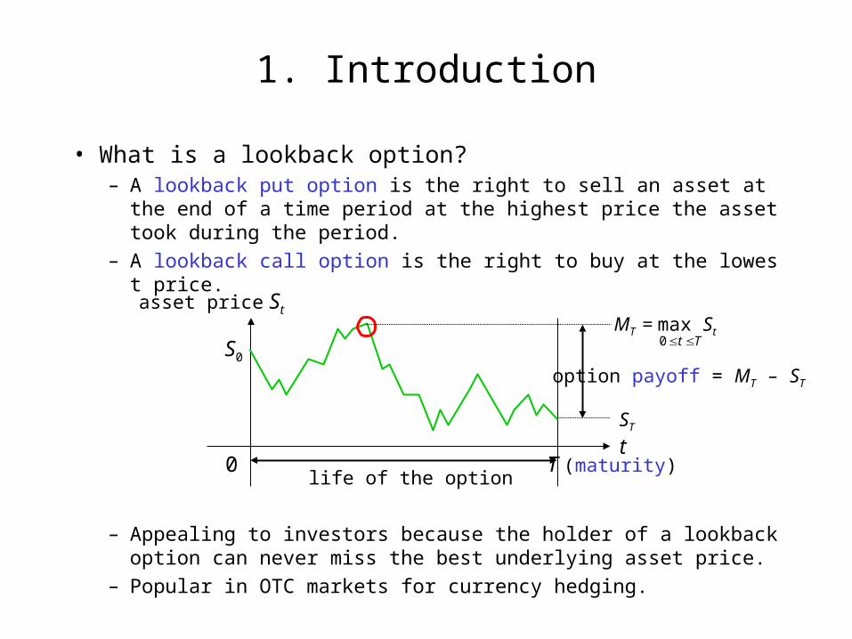
1. Introduction

• What is a lookback option? – A lookback put option is the right to sell an asset at the end of a ti

me period at the highest price the asset took during the period.

– A lookback call option is the right to buy at the lowest price.

– Appealing to investors because the holder of a lookback option can never miss the best underlying asset price.

– Popular in OTC markets for currency hedging.

asset price St

tT (maturity)

S0

0life of the option

option payoff = MT – ST

ST

MT = max St Tt 0

Pricing of lookback options

• The option price– Though lookback options give the buyer great flexibility, the seller (the counter party

of the option contract) has to take on a lot of risk.– To compensate for the risk, the buyer of the option has to pay the seller at the beginn

ing of the contract. This is called the option price.

• The pricing principle– The rational option price is given as the discounted expectation value (under the risk-

neutral probability) of the option payoff:

• Analytical formula– When the asset follows the Black-Scholes model dSt/St = r dt + dWt and the extreme v

alues are continuously monitored, analytical pricing formula is available . (Conze and Viswanathan, 1991)

V0(S0) = e–rT E0[MT – ST].

Pricing of discrete lookback options

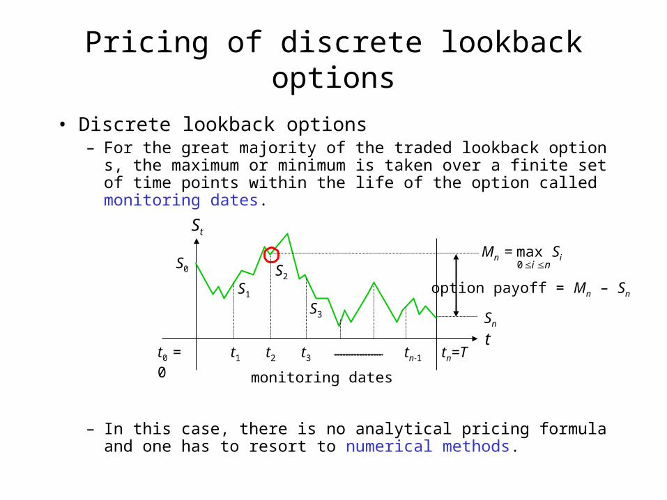
• Discrete lookback options– For the great majority of the traded lookback options, the maximu

m or minimum is taken over a finite set of time points within the life of the option called monitoring dates.

– In this case, there is no analytical pricing formula and one has to resort to numerical methods.

St

t

S0

monitoring dates

option payoff = Mn – Sn

Sn

Mn = max Sini 0

t1 t2 t3 tn-1 tn=Tt0 = 0

S1

S2

S3

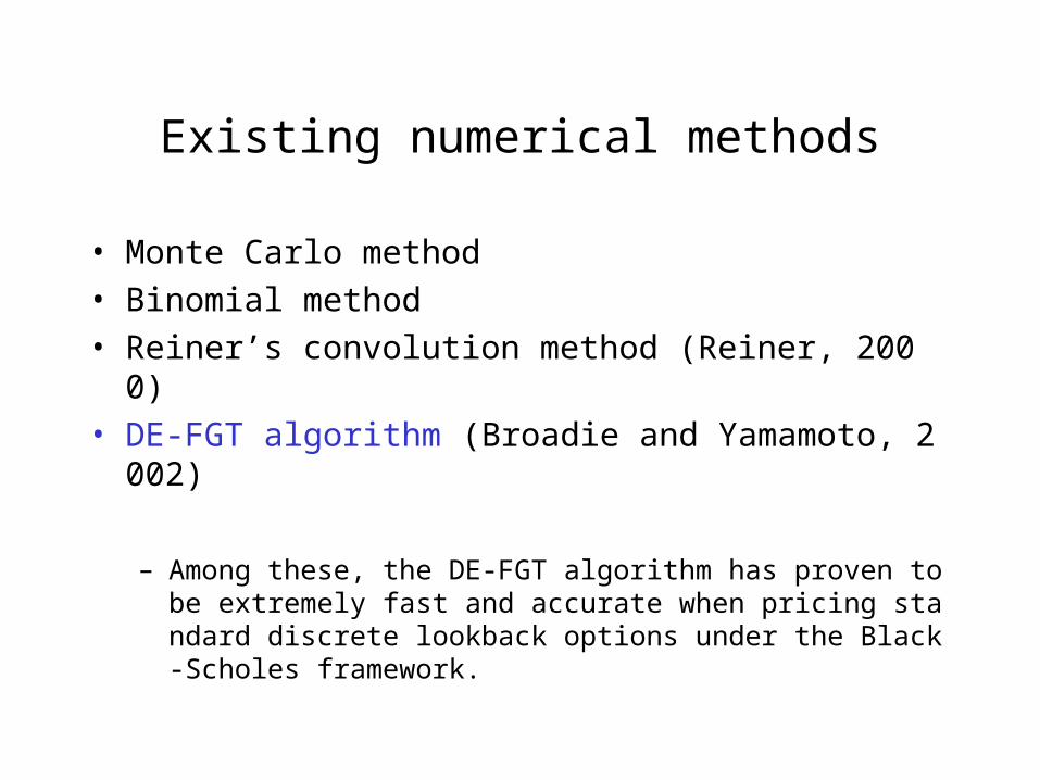
Existing numerical methods

• Monte Carlo method

• Binomial method

• Reiner’s convolution method (Reiner, 2000)

• DE-FGT algorithm (Broadie and Yamamoto, 2002)

– Among these, the DE-FGT algorithm has proven to be extremely fast and accurate when pricing standard discrete lookback options under the Black-Scholes framework.

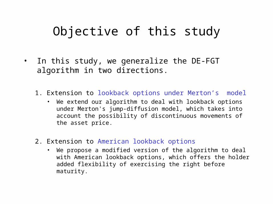
Objective of this study

• In this study, we generalize the DE-FGT algorithm in two directions.

1. Extension to lookback options under Merton’s model• We extend our algorithm to deal with lookback options under

Merton's jump-diffusion model, which takes into account the possibility of discontinuous movements of the asset price.

2. Extension to American lookback options• We propose a modified version of the algorithm to deal with

American lookback options, which offers the holder added flexibility of exercising the right before maturity.

2. The DE-FGT algorithm for lookback options

• Problem formulation– Let’s consider a discrete lookback put option with time period [0, T]

and n+1 monitoring dates ti = it (i = 0, 1, …, n, t = T/n).– Assume also that the asset price follows the Black-Scholes model:

– and let• Si = (asset price at ti) and• Mi = max Sk.

– Then the option price is given as the discounted expectation value of the option payoff:

dSt / St = (r – q) dt + dWt (r: interest rate, q: dividend rate,: volatility,Wt : standard Brownian motion)

ik 0

V0(S0) = e–rT E0[Mn – Sn].

Computation of the expectation value

• Reduction to a 1-dimensional problem– To evaluate the expectation value, we need the joint probability de

nsity function (pdf) of Sn and Mn.

– To reduce the dimensionality, we apply a change of measure (Babbs, 1992):

and obtain a new expression:

– By introducing log stock prices by si = log(Si /S0) and mi=log(Mi /S0),

– So we only need the probability density function of mn – sn.

V0(S0) .

V0(S0)

Computing the pdf of mn – sn

• The recurrence formula– To compute the pdf of mn – sn, we use the following relation:

– If the asset follows a Levy process, mi–1– si–1 is independent of si–1– si.

– The pdf of (mi–1– si–1) + (si–1– si) can be computed as the convolution of the pdf’s of mi–1– si–1 and si–1– si.

– Finally, the pdf of mi– si is obtained by collecting all the probability mass corresponding to mi– si < 0 to the point mi– si = 0 .

• As a result, the pdf of mi– si has a -function component at mi– si = 0.

Computing the pdf of mn – sn (cont’d)

• The recurrence formula (cont’d)– By expressing the pdf of mi– si as ci(x) + gi(x), we have the recurrence fo

rmula:

where c0 = 1, gi(x) = 0 and f (x) is the pdf of si–1– si.– Under the BS model, si–1– si follows Gaussian distribution N(–(r – q – (1/2)2)t, 2). – The recurrence formula reduces to convolution of a given function with

Gaussian.

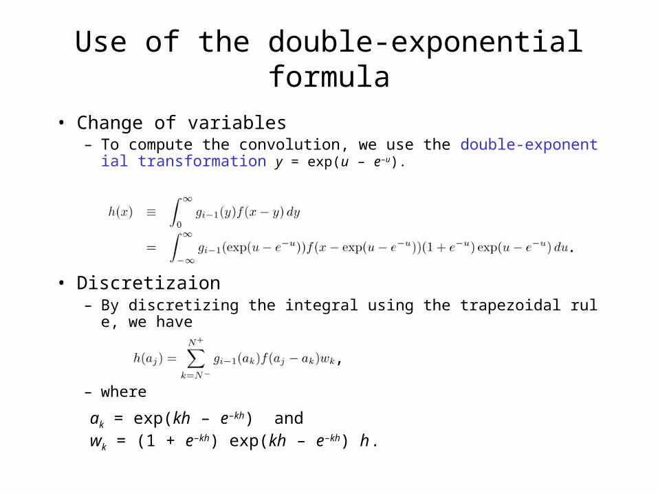
Use of the double-exponential formula

• Change of variables– To compute the convolution, we use the double-exponential transf

ormation y = exp(u – e–u).

• Discretizaion– By discretizing the integral using the trapezoidal rule, we have

– where

.

,

ak = exp(kh – e–kh) andwk = (1 + e–kh) exp(kh – e–kh) h .

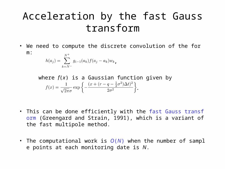
Acceleration by the fast Gauss transform

• We need to compute the discrete convolution of the form:

where f(x) is a Gaussian function given by

• This can be done efficiently with the fast Gauss transform (Greengard and Strain, 1991), which is a variant of the fast multipole method.

• The computational work is O(N) when the number of sample points at each monitoring date is N.

,

.

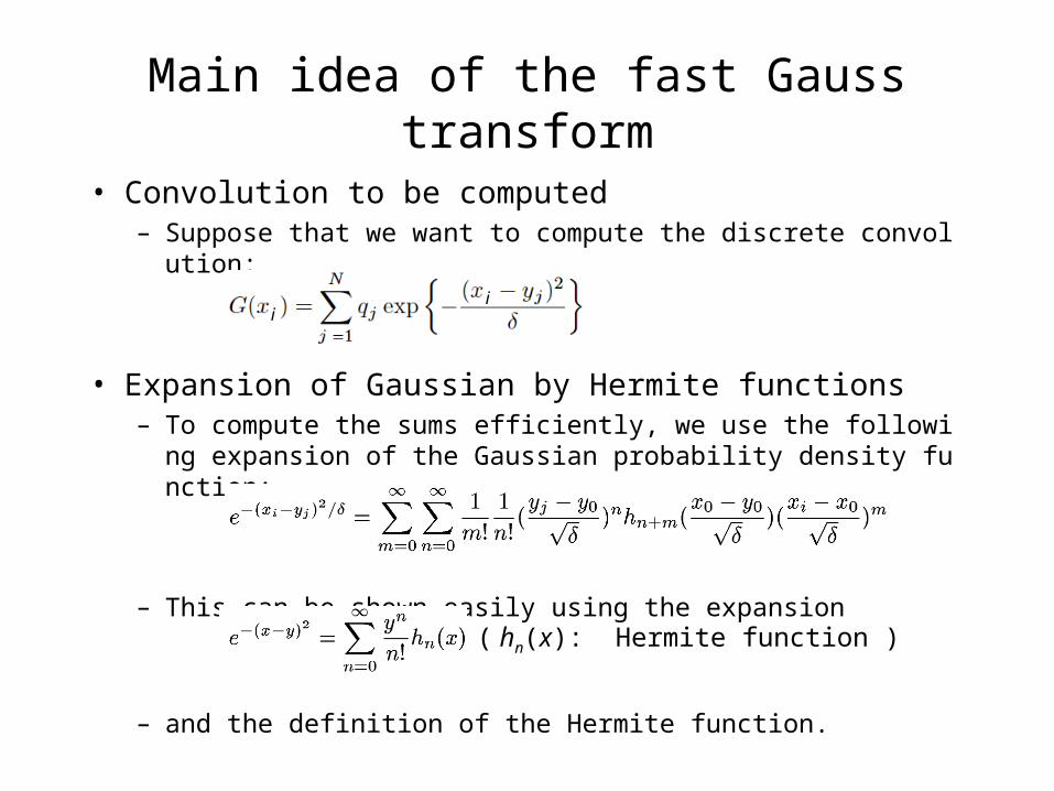
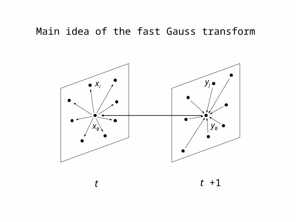
Main idea of the fast Gauss transform

• Convolution to be computed– Suppose that we want to compute the discrete convolution:

• Expansion of Gaussian by Hermite functions– To compute the sums efficiently, we use the following expansion o

f the Gaussian probability density function:

– This can be shown easily using the expansion

– and the definition of the Hermite function.

( hn(x): Hermite function )

ii

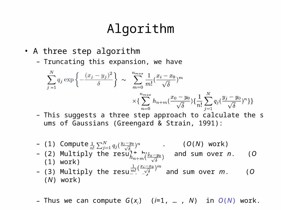
Algorithm

• A three step algorithm– Truncating this expansion, we have

– This suggests a three step approach to calculate the sums of Gaussians (Greengard & Strain, 1991):

– (1) Compute . (O(N) work)

– (2) Multiply the result by and sum over n. (O(1) work)

– (3) Multiply the result by and sum over m. (O(N) work)

– Thus we can compute G(xi) (i=1, … , N) in O(N) work.

ii

Main idea of the fast Gauss transform

t t +1

yj

y0

xi

x0

Acceleration by the fast Gauss transform

• We need to compute the discrete convolution of the form:

where f(x) is a Gaussian function given by

• This can be done efficiently with the fast Gauss transform (Greengard and Strain, 1991), which is a variant of the fast multipole method.

• The computational work is O(N) when the number of sample points at each monitoring date is N.

,

.

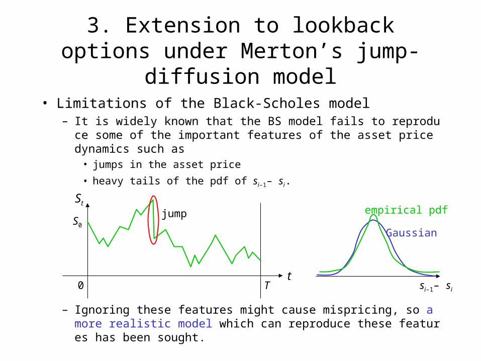
3. Extension to lookback options under Merton’s jump-diffusion model

• Limitations of the Black-Scholes model– It is widely known that the BS model fails to reproduce some of th

e important features of the asset price dynamics such as• jumps in the asset price

• heavy tails of the pdf of si–1– si.

– Ignoring these features might cause mispricing, so a more realistic model which can reproduce these features has been sought.

St

t

S0

T0

jump

Gaussian

empirical pdf

si–1– si

Merton’s jump-diffusion model

• The model– Merton’s jump-diffusion model (Merton, 1976) is the simplest mo

del that can reproduce these features.– It adds random jumps driven by a Poisson process to the BS mode

l.– The size of jumps is also random and is log-normally distributed.

• SDE for the asset price

– where• N(t) : Poisson process with intensity .• Vl: i.i.d. random variables such that log(Vl) follows N (, 2).

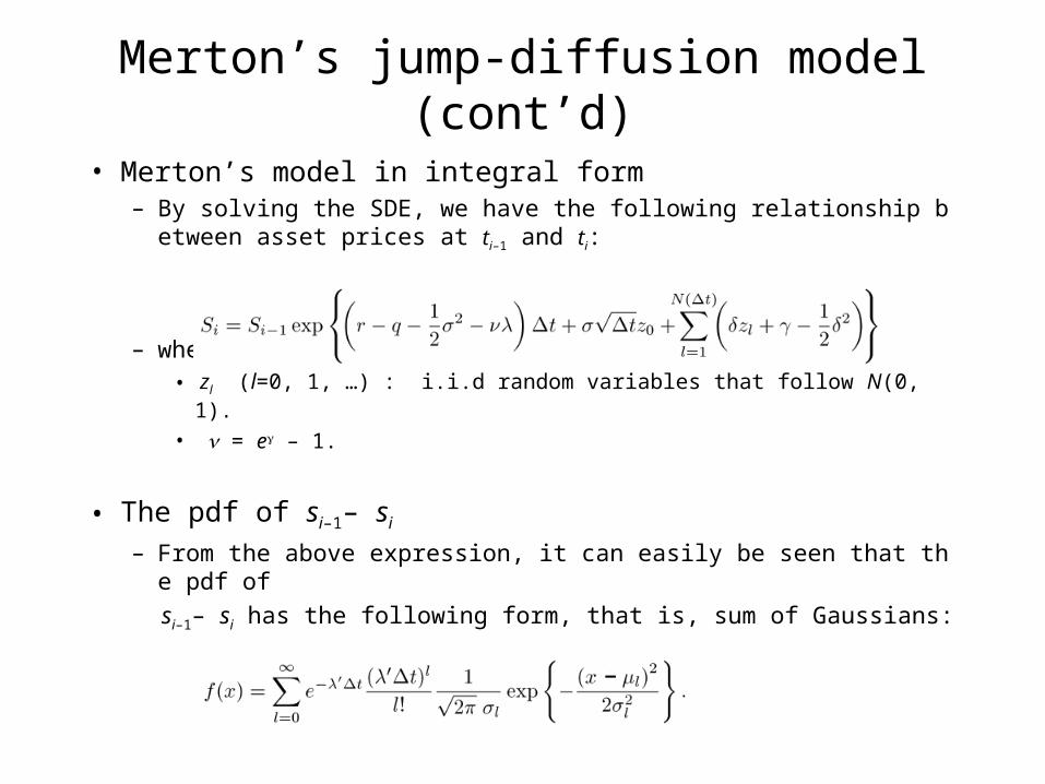
Merton’s jump-diffusion model (cont’d)

• Merton’s model in integral form– By solving the SDE, we have the following relationship between a

sset prices at ti–1 and ti:

– where• zl (l=0, 1, …) : i.i.d random variables that follow N(0,1).

• = e – 1.

• The pdf of si–1– si

– From the above expression, it can easily be seen that the pdf of

si–1– si has the following form, that is, sum of Gaussians:–

Computing the lookback option price

• Reduction to a 1-dimensional problem– To compute the lookback option price, we first apply the change of measure to reduce

the dimensionality of the problem:

– Then we can write the option value (as in the BS case) as follows:

– Under the new measure Q’, the asset price can be shown to follow a new jump-diffusion process with modified parameters:

The functional form of f(x) does not change.

– This can be proved using Girsanov’s theorem for jump-diffusion processes. An elementary proof can also be given.

V0(S0)

r’ = r + 2, ’ = + 2, ’ = e

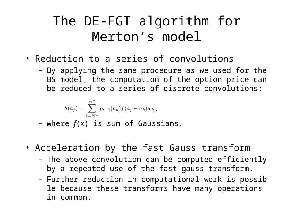
The DE-FGT algorithm for Merton’s model

• Reduction to a series of convolutions– By applying the same procedure as we used for the BS model, the

computation of the option price can be reduced to a series of discrete convolutions:

– where f(x) is sum of Gaussians.

• Acceleration by the fast Gauss transform– The above convolution can be computed efficiently by a repeated

use of the fast gauss transform.

– Further reduction in computational work is possible because these transforms have many operations in common.

,

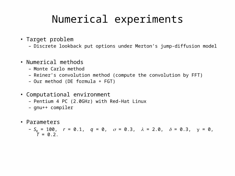
Numerical experiments

• Target problem– Discrete lookback put options under Merton’s jump-diffusion model

• Numerical methods– Monte Carlo method– Reiner’s convolution method (compute the convolution by FFT)– Our method (DE formula + FGT)

• Computational environment– Pentium 4 PC (2.0GHz) with Red-Hat Linux – gnu++ compiler

• Parameters– S0 = 100, r = 0.1, q = 0, = 0.3, = 2.0, = 0.3, = 0, T = 0.2.

1.E-09

1.E-08

1.E-07

1.E-06

1.E-05

1.E-04

1.E-03

1.E-02

1.E-01

1.E+00

1.E+01

0.1 1 10 100 1000

ReinerMonte Carlo

DE-FGT

Numerical results

Computation time (sec)

The DE-FGT method outperforms Reiner’s convolution method and the Monte Carlo method in this case.

It can compute the price of the lookback option price within 0.4 seconds up to the accuracy of 10-9.

Results for an option with 25 monitoring dates (extremum monitored every two days)

Option price = 12.09911864

Abs

olut

e er

ror

1.E-10

1.E-09

1.E-08

1.E-07

1.E-06

1.E-05

1.E-04

1.E-03

1.E-02

1.E-01

1.E+00

1.E+01

0.1 1 10 100 1000

ReinerMonte Carlo

DE-FGT

Numerical results (cont’d)A

bsol

ute

erro

r

Computation time (sec)

The behavior of the three numerical methods are almost the same as for the n=25 case.

The DE-FGT algorithm can compute the price of the lookback option price within 1.0 seconds up to the accuracy of 10-9.

Results for an option with 50 monitoring dates (daily monitoring).

Option price = 12.57499665

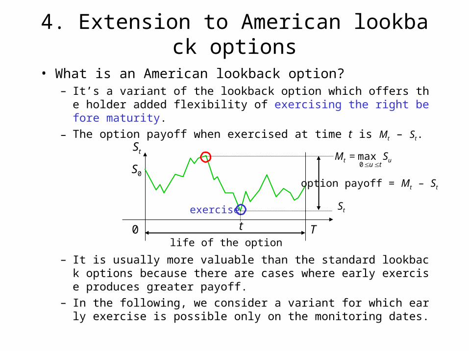
4. Extension to American lookback options

• What is an American lookback option?– It’s a variant of the lookback option which offers the holder added

flexibility of exercising the right before maturity.

– The option payoff when exercised at time t is Mt – St.

– It is usually more valuable than the standard lookback options because there are cases where early exercise produces greater payoff.

– In the following, we consider a variant for which early exercise is possible only on the monitoring dates.

St

t T

S0

0life of the option

option payoff = Mt – St

St

Mt = max Su tu 0

exercise

Pricing of the American lookback options

• Pricing principle– It is known that the rational price of the American lookback option

is given by the following expression (cf. Duffie, 1996):

V0(S0) = sup E0[e–rt (M – S)]

– Here, denotes Markov stopping time.

– That is, we consider expectation values under all possible stopping times (i.e. exercise strategies) and take the supremum.

Pricing by dynamic programming

• To compute this expectation value, we use dynamic programming and use the backward recursion:

Vi(Si, Mi) = max (Mi – Si, e–rt Ei[Vi+1] )

where– Vi is the option value at time ti and is a function of Mi and Si in general.– Ei is the expectation value operator given information up to ti.

• For i = n, we have Vn = Mn – Sn.

• This backward recursion reflects the strategy of exercising the right when the “immediate exercise value” is greater than the discounted expected value of the option at the next monitoring date, and holding the right otherwise.

immediate exercise value continuation value

Reduction to a 1-dimensional problem

• Change of measure– To reduce the dimensionality of the problem, we introduce a new

variable Vi’ = Vi/Si and rewrite the backward recursion formula:

– B further introducing a change of measure similar to the one used for standard lookback options, we have

– Inserting this into the above formula, we have a new recursion:

– Furthermore, it can be shown that Vi’ (Si, Mi) is a function of Mi / Si only. Thus we have reached a 1-diemnsional problem.

Vi(Si, Mi) = max (Mi – Si, e–rt Ei[Vi+1] )

Vi’ (Si, Mi) = max (Mi / Si – 1, e–rt Ei[Vi+1] / Si ).

Vi’ (Si, Mi) = max (Mi / Si – 1, e–qt Ei’ [Vi+1]).

e–rt Ei[Vi+1] = Si e–qt Ei’ [Vi+1/Si+1]

Application of the DE-FGT method

• The main task in computing the recursion

is the evaluation of the expectation value Ei’ [Vi+1] for each value of Mi / Si.

• By introducing the log stock prices by si = log(Si /S0) and mi=log(Mi /S0) (as in the case of standard lookback options), this can be rewritten as a convolution of a function with Gaussian.

• Then our DE-FGT method can be applied.

Vi’ (Si, Mi) = max (Mi / Si – 1, e–qt Ei’ [Vi+1]).

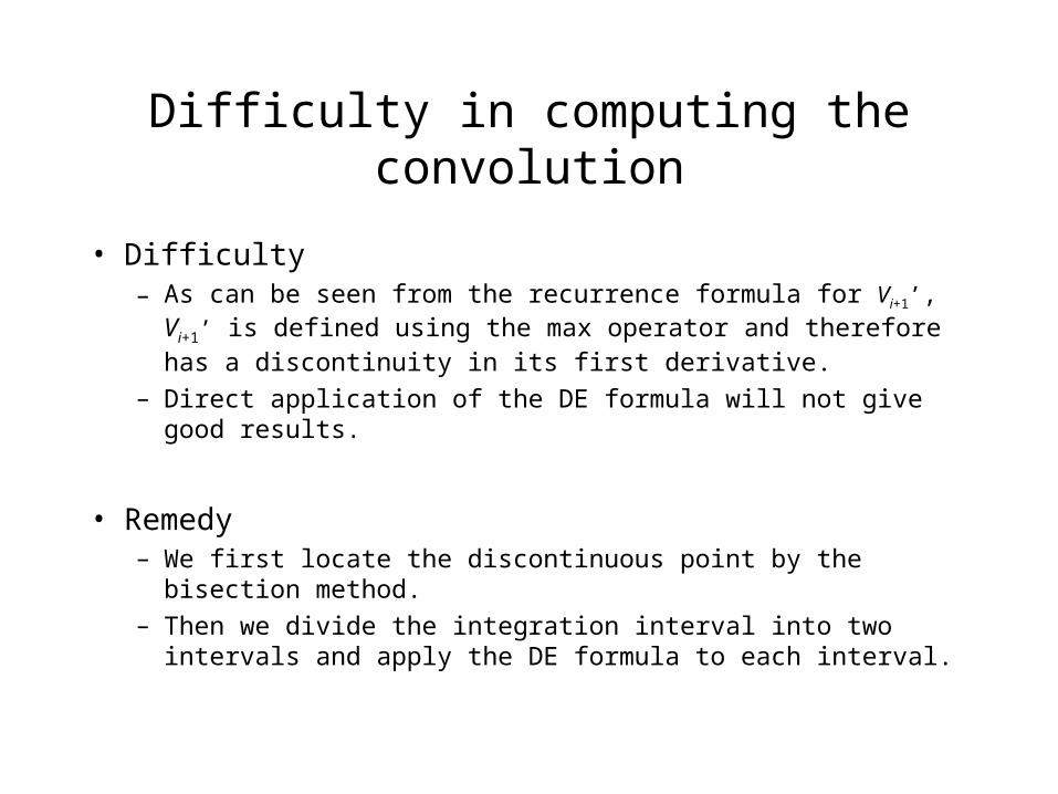
Difficulty in computing the convolution

• Difficulty– As can be seen from the recurrence formula for Vi+1’, Vi+1’ is

defined using the max operator and therefore has a discontinuity in its first derivative.

– Direct application of the DE formula will not give good results.

• Remedy– We first locate the discontinuous point by the bisection method.

– Then we divide the integration interval into two intervals and apply the DE formula to each interval.

Numerical experiments

• Target problem– Discrete American lookback put options under Black-Scholes model

• Numerical methods– Binomial method– Reiner’s convolution method– Our method (DE formula + FGT)

• Computational environment– Same as the previous numerical experiments

• Parameters– S0 = 100, r = 0.1, q = 0, = 0.3, T = 0.2.

1.E-09

1.E-08

1.E-07

1.E-06

1.E-05

1.E-04

1.E-03

1.E-02

1.E-01

1.E+00

0.01 0.1 1 10 100

ReinerBinomial

DE-FGT

Numerical results

Computation time (sec)

Results for an option with 5 monitoring /exercise dates (bi-weekly monitoring/exercise)

Option price = 7.05538954

Abs

olut

e er

ror

The convergence of Reiner’s method is rather irregular. This seems to be because of the discontinuity in the first derivative of the integrand function.

1.E-09

1.E-08

1.E-07

1.E-06

1.E-05

1.E-04

1.E-03

1.E-02

1.E-01

1.E+00

0.01 0.1 1 10 100

ReinerBinomial

DE-FGT

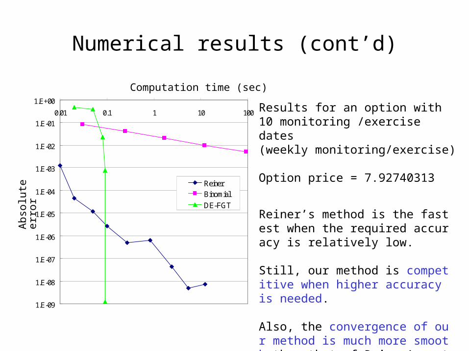
Numerical results (cont’d)

Computation time (sec)

Reiner’s method is the fastest when the required accuracy is relatively low.

Still, our method is competitive when higher accuracy is needed.

Also, the convergence of our method is much more smooth than that of Reiner’s method.

Results for an option with 10 monitoring /exercise dates (weekly monitoring/exercise)

Option price = 7.92740313

Abs

olut

e er

ror

5. Conclusion

• We proposed a pricing algorithm based on the DE formula and the fast Gauss transform for lookback options under Merton’s model and American lookback options.

• For lookback options under Merton’s model, our method outperforms conventional methods such as Reiner’s convolution method and can compute the option price within 1 second up to accuracy of 10–9.

• For American lookback options, reiner’s method is the fastest when the required accuracy is relatively low. But our method is competitive when high accuracy is required.

Future work

• Extension to more general jump-diffusion asset price models– variance gamma models

– stochastic volatility models

• Extensions to other types of exotic options– options on two or more assets

– various path-dependent options