Doppler Lidar Research at ASU - University of Utahwhiteman/metcrax2/images/kickoff/Lidars... ·...
23
Doppler Lidar Research at ASU Jan. 23, 2013 METCRAX II - Kickoff Ronald Calhoun Associate Professor Environmental Remote Sensing Group Department of Mechanical & Aerospace Engineering Senior Sustainability Scientist, School of Sustainability ASU Arizona State University
Transcript of Doppler Lidar Research at ASU - University of Utahwhiteman/metcrax2/images/kickoff/Lidars... ·...

Doppler Lidar Research at ASU
Jan. 23, 2013 METCRAX II - Kickoff
Ronald Calhoun
Associate Professor Environmental Remote Sensing Group
Department of Mechanical & Aerospace Engineering Senior Sustainability Scientist, School of Sustainability ASU
Arizona State University

Environmental Remote Sensing Group I. LIDAR Group - Background
Established Record (ASU lidar): • ~ 10 years research in Lidar Data Analysis • ~ $3.7 million of research, • 31 Journals articles, • 72 conference presentation/papers, • 30 invited talks…
Current Research Projects: • DOE Offshore Wind Project • INTEL – Wind Farm Control • Lockheed Martin – Dual Doppler Validation • NASA – Aircraft Vortex Tracking • National Science Foundation – Nocturnal Flows • National Science Foundation –Canopy Flow
History • Africa & Colorado Demonstration Projects • Ongoing Dual Doppler – Boulder, CO Directions • Offshore Demonstration of WRA • Wind Farm Control Algorithm Testing
3D Scanning Doppler Lidar (Type LM: WINDTRACER)
Lidar data overlay for ACUA Deployment New Jersey

Environmental Remote Sensing Group- last 10 years • ARO – DURIP: Acquisition of WindTracer • Lawrence Livermore National Laboratory: Advanced sensor integration into NARAC • ARO: JU2003 Deployment • WERF: Airborne biological contaminants associated with land applied biosolids • ARO: Air flow and dispersion over an Urban downtown area (JU2003 Analysis) • NSF: Data assimilation of dual Doppler lidar observations of the urban bound. layer • ARO: Acquisition of a Sodar/RASS Instrument for Remote Sensing of Urb. Environ… • NSF: Coherent Doppler lidar deployment and data analysis for T-REX • ARO: Stable boundary layer analysis – T-REX • Western Australian Department of the Environment: Pathways of Pollution Exposure • ARO: Sedona workshop on the atmospheric stable boundary layer • Arizona Dept. Environ. Quality: Tracking PM-10 using coherent Doppler Lidar • ARO: Doppler Lidar Deployment for the Canopy Horizontal Array Turbulence Study • TABLES – scintillometry and temperature/humidity lidar over Swiss lake. • Kenya Wind Project – Doppler lidar deployment for wind resource assessment • NASA Wake Vortex • NSF Lidar Analysis for Canopy Studty (CHATS) • DOE Offshore Wind Measurements • Feasibility study wind farm control & optimization • METCRAX-II Wind Flow over a Crater

Courtesy of LMCT
ASU Laser Radar Equipment (2 lidars): • Windtracer, LMCT, 2 micron system • Windtracer, LMCT, 1.6 micron system

Horizontal velocity vectors from OI technique on a 3.5o elevation conical scan showing the rotation of winds with height. The colors on the plot represent radial velocity measurements by lidar. Red color (positive values) represent wind moving away from the lidar and blue color (negative values) shows wind moving towards the lidar. Data with low SNR is not shown (white regions). See Choukulkar et al. 2012

Town
Plume Source
Alcoa Aluminium Refinery
Wagerup, Australia Alcoa has proposed a $A 1.5 billion expansion of the Wagerup refinery. – Now on hold….
~ 5 Kilometers

The PPI (2.5 degrees) at 8:09. The view is toward the northeast, again note the break in the PPI is at zero degrees.
Backscatter on August 27th, 2006

These two figures show 2.5 degree RHI backscatter plots for 5:39 and 6:27 a.m. on August 29th, 2006.
Two PPI’s at 6:48 and 6:57 a.m. on August 29th, 2006.

RHI’s looking eastward toward escarpment at successively larger angles. Radial velocity on left and backscatter is on the right. Time progresses according to typical scanning pattern after approximately 8:32 a.m.

Radial velocities on 2.5 degree PPI’s at 5:27, 5:48, 6:18, 6:39, 6:48, and 7:09 a.m. on August 29th, 2006. Notice the counterclockwise rotation of the wind on the lowest levels near the center of the sub-plots.
Rotation of Lower Wind Direction
Conclusion: Must use radial velocity fields to diagnose representativeness of 2.5 degree PPI of backscatter for ground exposures.

Note continuity between elevated release and lower levels closer to lidar…
500 1000 1500 2000 2500 3000
200
400
600
800
1000
1200
1400
1600
1800
2000
PPI sweep:Date:8/27/2006 Time:8:21:54 AZ:39.9775
-9
-8.5
-8
-7.5
-7
-6.5
-6
Aerial Schematic
RHI Direction
“Fanning”
RHI’s indicate “Milling Vent” producing strong backscatter levels.

Terrain –induced Rotors Experiment TREX
Mar 1 – May 1 2006
Meteorological Overview (iii)
DLR PPI scan of radial velocity in ms-‐1 at an eleva8on angle of 5 degrees on Mar 25, 2006 at 6:29:00 am PST (14:29:00 UTC ). Flow is south to north flow, along the 345 degree azimuth with a maximum magnitude of 11 to 12 m s-‐1.
• South to North flow driven by
the pressure gradient.

Meteorological Overview (iv)
DLR PPI radial velocity scan in m s-‐1 at an eleva=on angle of 10 degrees at 8:59:50 am PST (16:59:50 UTC). Flow is south to north along 350 azimuth. Maximum velocity ~10 m s-‐1. Note the incoming pulse of the wind from the west over the mountains.
• South to North flow driven by the pressure gradient.
• Westerly flow descending over the mountain topography to the west.

Meteorological Overview (v)
DLR PPI radial velocity scan in ms-‐1 at an eleva8on angle of 10 degrees at 9:29:49 am PST (17:29:49 UTC). Flow is southwest to northeast along the 40 degree azimuthal direc8on, and with a velocity maximum velocity of ~13 m s-‐1. The mean flow has become cross-‐valley, and the lower up-‐valley mean flow has been destroyed.
• Prevailing westerly flow has broken up the pressure driven
flow at the lowest altitudes.

DLR ASU
2.9 km 9.1 km 10.9 km
Lidar Scanning Configura8on
• Coplanar scans along 80 degree azimuth • Height difference: Zdlr – Zasu ~ 63.5 m

Retrieval of Rotors From T-REX


Smaller mo=ons: sub-‐rotors • Sub-‐rotor Characteris=cs
– Usually at least 300 m in diameter.
– Vor=city/Swirl above 0.02 s-‐1.
– Advects with the mean flow.
– When isolated above 2.6 km agl, sub-‐rotors typically have nega=ve orienta=on.
– Below 2.0 km agl, may have posi=ve or nega=ve orienta=on.
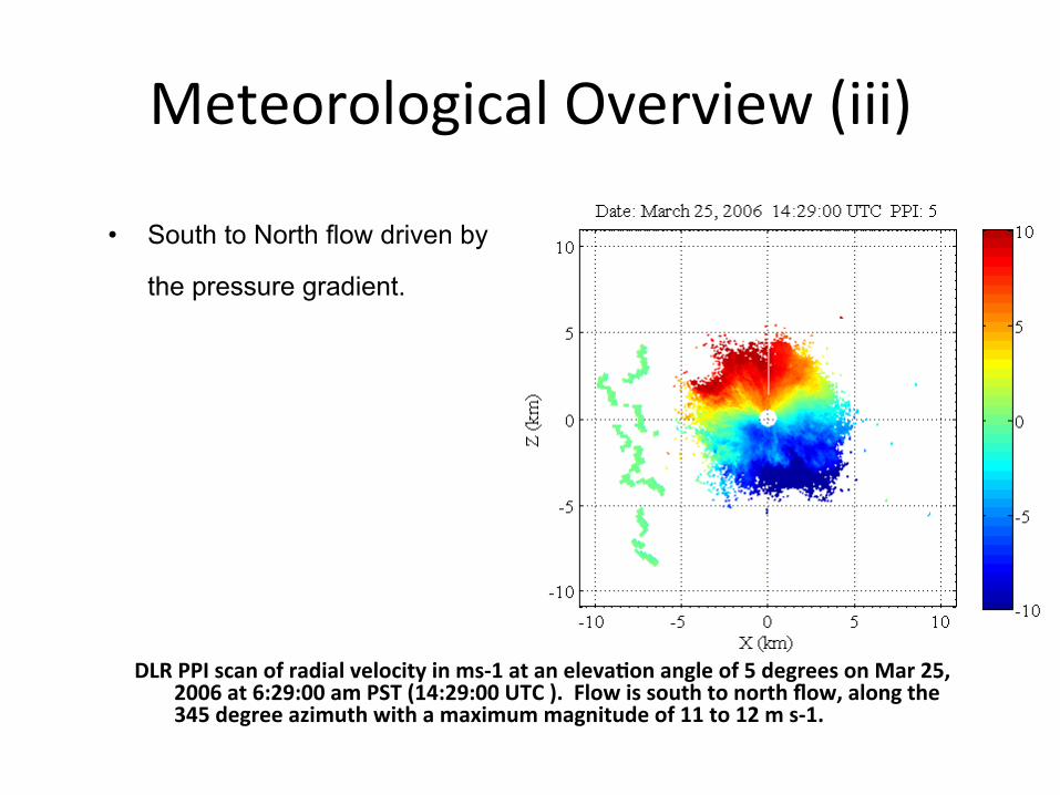
Streamlines (with arrows), vorticity and swirling strength (contours without arrows) for the rotor at 11:09 am PST (1909 UTC). Units are in s-1. [Hill et al. 2010, Journal of the Atmospheric Sciences.]

Larger Coherent Mo=ons: Rotors • Rotor Characteris=cs
– 1+ km in diameter. – Complete circula=on,
connec=on of streamlines.
– Same approximate loca=on on the order of minutes.
– May contain smaller vor=ces (with nega=ve vor=city) within the larger circula=on.
– Preceded/accompanied by lee wave or gravity current.
– Principally nega=ve rota=on (clockwise)
Vorticity and swirling strength (contours without arrows) for the rotor at 11:04 am PST (1904 UTC) with the accompanying streamlines (with arrows).
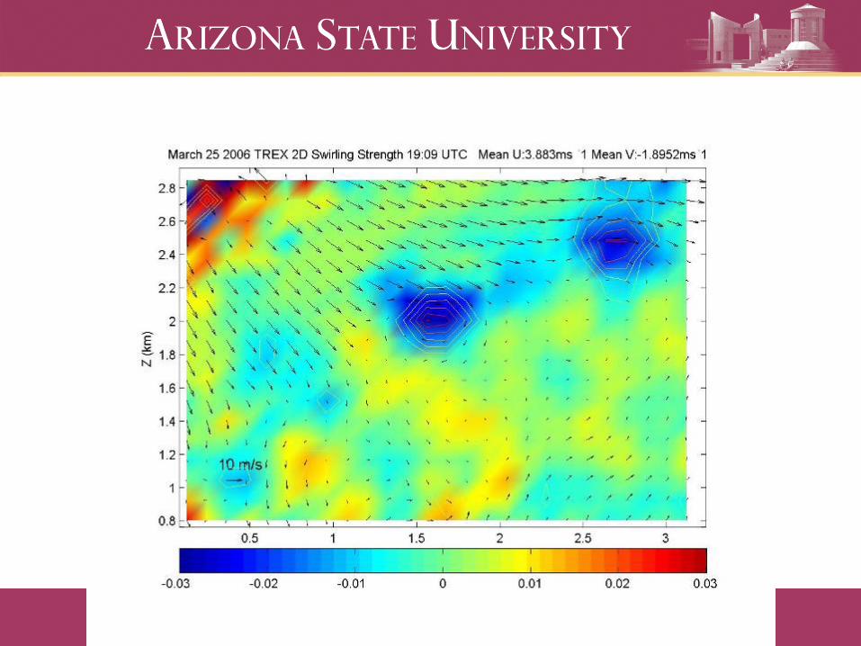
Noise Pollu=on of Rotor at 11:04 am PST
Vorticity, swirl, and streamline subplots at 11:04 am PST (1904 UTC) with increasing levels of gaussian zero mean noise. Mean domain velocity <u> is approximately 5.5 ms-1. Noise magnitude
indicated by standard deviation, σNoise. a) No noise b) σNoise = 1.00 ms-1 and σNoise /<u> = 0.18 d) σNoise = 2.00 ms-1 and σNoise/<u> = 0.36, and d) σNoise = 3.00 ms-1 and σNoise/<u> = 0.54.
a
d c
b