Doppler effect on target tracking in wireless sensor...

Computer Communications 36 (2013) 834–848

Contents lists available at SciVerse ScienceDirect

Computer Communications

journal homepage: www.elsevier .com/ locate/comcom

Doppler effect on target tracking in wireless sensor networks

0140-3664/$ - see front matter � 2013 Elsevier B.V. All rights reserved.http://dx.doi.org/10.1016/j.comcom.2013.01.002

⇑ Corresponding author. Tel.: +1 256 824 6858.E-mail addresses: [email protected] (Y.K. An), [email protected] (S.-M. Yoo),

[email protected] (C. An), [email protected] (B. Earl Wells).

Youngwon Kim An a, Seong-Moo Yoo a,⇑, Changhyuk An b, B. Earl Wells a

a Department of Electrical and Computer Engineering, The University of Alabama in Huntsville, Huntsville, AL 35899, United Statesb PRA, Huntsville, AL 35801, United States

a r t i c l e i n f o a b s t r a c t

Article history:Received 27 April 2012Received in revised form 17 December 2012Accepted 2 January 2013Available online 10 January 2013

Keywords:Wireless sensor networksDoppler effectKalman filterTrackingDetection

This paper presents a new detection algorithm and high speed/accuracy tracker for tracking ground tar-gets in acoustic wireless sensor networks (WSNs). Our detection algorithm naturally accounts for theDoppler effect which is an important consideration for tracking higher-speed targets. This algorithmemploys Kalman filtering (KF) with the weighted sensor position centroid being used as the target posi-tion measurement. The weighted centroid makes the tracker to be independent of the detection modeland changes the tracker to be near optimal, at least within the detection parameters used in this study.Our approach contrasts with previous approaches that employ more sophisticated tracking algorithmswith higher computational complexity and use a power law detection model. The power law detectionmodel is valid only for low speed targets and is susceptible to mismatch with detection by the sensorsin the field. Our tracking model also enables us to uniquely study various environmental effects on trackaccuracy, such as the Doppler effect, signal collision, signal delay, and different sampling time. Our WSNtracking model is shown to be highly accurate for a moving target in both linear and accelerated motions.The computing speed is estimated to be 50–100 times faster than the previous more sophisticated meth-ods and track accuracy compares very favorably.

� 2013 Elsevier B.V. All rights reserved.

1. Introduction

Recent advancements of micro sensors technology have al-lowed a wide range of wireless sensor networks (WSNs) imple-mentations to be realized. WSNs are used in monitoring anddetecting specific events in many types of industrial and militaryenvironments. They are especially useful in such situations astracking emergency rescue workers, tracking military targets inmodern battlefield scenerios, and monitoring traffic in transporta-tion systems [1].

WSNs, in general, are composed of a large number of micro sen-sors and a base station. Each micro sensor is battery powered andis constructed using analog sensor, microcontroller, memory, andcommunication component subunits. A WSN acoustic tracking sys-tem, the main subject of this paper, includes two parts. One con-sists of acoustic sensors which are distributed in a uniform grid(or some other known configuration) to detect target sound. Theother is the fusion center where target detection information fromthe sensors is processed to track the target. In general, these sen-sors are not capable of performing complicated computation andcommunication because of the limited power and computing re-sources that are present at each node. Each sensor uses a single

bit to indicate that a target had been detected. When the sensor de-tects target sound power that is higher than a predeterminedthreshold value, it sends the detection information bit along withits ID and sound power information to the fusion center, otherwiseit sends no information. The fusion center receives the signals fromthe sensors and records the receiving time along with the sensor IDand sound power information. Based upon the particular sensorlayout, each sensor ID is translated into a corresponding target po-sition that can be used along with the sound power information fortracking the target using a wide range of tracking methods.

1.1. Previous studies

A number of tracking methods for a single target trackinghave been proposed in the literature for WSN type applications.Mechitov et al. [1] and Kim et al. [2] used a path based approachthat used the detection duration of each sensor as a weight andperformed line fitting in a time window to estimate target positionat each time step. The requirement of using detection durationinformation from each sensor may be a hindrance for real timeapplication of the algorithm and reliable line fitting may requirea high sampling rate by each sensor. Both methods also need timesynchronization and information exchange between neighboringsensors and thus tend to further impose computing and communi-cation loads to each sensor. Wang et al. [3,4] used a similar geo-metric method for target position estimation which requires each

http://dx.doi.org/10.1016/j.comcom.2013.01.002

mailto:[email protected]




http://dx.doi.org/10.1016/j.comcom.2013.01.002

http://www.sciencedirect.com/science/journal/01403664

http://www.elsevier.com/locate/comcom

Y.K. An et al. / Computer Communications 36 (2013) 834–848 835

sensor to store neighbor node identifier, intersection points ofsensing circle of the node and its neighbor and an angle corre-sponding to the arc defined by these intersection points of thesensing circle. In noisy real-world environments accurate estima-tion of these parameters may be challenging. Also the applicabilityof the method to a target with a short sensing range covering onlyone or zero sensor or with a long sensing range covering many sen-sors is to be seen.

Ribeiro et al. [5] developed Kalman filter (KF) based recursivealgorithms for distributed state estimate based on the sign of inno-vations (SOI). Running the SOI-KF requires each sensor to detectthe target sound, compute the state and observation predicted esti-mate, obtain SOI and send the information to all other sensors forcomputing the updated state. As each sensor has limited powerand limited computing and communication resources, this algo-rithm may give too much load to each of the sensor nodes.

Recently, a number of authors [6–8,11] chose the particle filters(PFs) over KF for target tracking in WSN environments. They claimthat KF is not an optimal filter as the system and measurementprocess are not linear and Gaussian in real environments. PFs havebecome one of the most popular methods for stochastic dynamicestimation problems and the PFs can handle nonlinear/non-Gaussian measurements and dynamics of target with highaccuracy but at the expense of computational complexity [10].For the application of PF to WSN, PFs with lower computationalcomplexity were proposed [22,23] but the error propagationthrough the sensor network was regarded as the main drawbackof the methods [9]. Similar results are reported by other authors[12–19]. As an improvement over PF, Teng et al. [9] applied avariational filter (VF) for target tracking. The filter uses a MonteCarlo method for a set of weighted samples to approximate theposterior distribution and adapts the variational approach. Theauthors claim that the algorithm is able to track targets in nearrandom motion with high accuracy.

All the previous studies mentioned above use the power law forsimulating target sound power detection by the sensors and usethe same power law for modeling the detection in their trackers.Their use of power law excludes the Doppler effect so that theirdetection model and track results are applicable only for verylow speed targets. The power law model also makes the detectionmodel in their tracker susceptible to mismatch with the detectionby the sensors deployed in real environment [8]. Even though theirchoice of trackers yields high track accuracy in their simulation,their trackers do not guarantee the same accuracy when it is usedfor real WSN environments because of the mismatch. Furthermore,their computational complexity, especially for PF and VF, is toohigh that their trackers may be costly for real world WSN system.

1.2. Contribution of this paper

The main contribution of this paper is to develop a realisticdetection algorithm where the Doppler effect appears naturallydepending on the target speed. For our tracker, we use the KF withthe weighted centroid of detecting sensor positions as target posi-tion measurement, which makes KF near optimal. None of the pre-vious studies used KF for acoustic WSN tracking systems, exceptthe case of distributed state [5,24], by reasoning that KF is not opti-mal in a variety of real world situations. The weighted centroid alsoallows the tracker to be independent of sound detection models sothat there is no detection mismatch between the tracker and thesensors in the field.

With our realistic detection model incorporated into KF, we cantrack high as well as low speed targets accurately with very lowcomputational complexity. The tracker also enables us to studyvarious environmental effects on track accuracy, including Dopplereffect, detection message delay and message collision at the fusion

center, and different sampling time steps. Our simulation study ofthese environmental effects demonstrates that the track accuracyis sensitive to these effects.

Using our KF, our track accuracy is comparable to the accuracyof PF and VF and the computing speed is estimated to be nearly 100times faster than the speed of those filters. The high computingspeed and high track accuracy are critical factors for implementingthe system in real world. This study is meant to lay the ground-work for more detailed systems study for implementing a WSNtracking system in real world scenarios.

This paper is organized as follows: Section 2 describes thedetection framework. It gives a detailed description of Doppler ef-fect in the sensor detection simulation. In Section 3, we describethe tracking framework demonstrating that KF becomes near opti-mal. An algorithm for tracking a target in acceleration is also pre-sented. In Section 4, we show the simulation results for trackaccuracy of target in linear and accelerated motions, and differentenvironmental effects. Section 5 compares our results with those ofprevious works. Section 6 concludes the paper.

2. Detection framework

We assume that the wireless sensors are simple passive sensorswithout range measurement capability. Each sensor has its ownunique integer ID that translates into its position. Each sensorhas own internal noise and also encounters ambient noise fromthe sensing region. A threshold value for the noises is set for eachsensor before the deployment. Target sound over the threshold va-lue will be detected by the sensor as a signal from a target and thedetection information will be sent to the fusion center.

2.1. Model for target sound propagation with Doppler effect

Most of previous studies modeled the received target soundpower using the following simple power law equation.

Ps;t ¼ P0;t=das;j þ ms;t ð1Þ

where P0,t is the target sound power at time t, Ps,t is the target soundpower detected by the sensor, s, at time t, and ms,t is the detectionnoise at the sensor s which is assumed to be a zero mean Gaussiandistribution. The distance from the sensor, s, to a target position at atime index j is expressed as ds,j in Eq. (2) and a is an attenuationparameter that depends on the environment of the sensing region.

d2s;j ¼ xs � xt

j

� �2þ ys � yt

j

� �2ð2Þ

Here, (xs, ys) is the sth sensor position and ðxtj ; y

tj Þ is the target posi-

tion at a time index j. If the detected target sound power, Ps,t is oneof measurement vector, the relationship between the measurement,~zs;t and target state vector, ~xt is a non-linear function as

~zs;t ¼ hð~xtÞ þ ms;t ð3Þ

Eq. (3) causes the Kalman filter (KF) to be suboptimal and then thePFs are appropriate for target tracking in WSN.

We note that Eq. (1) is not an accurate detection model for highspeed targets as the equation does not take into account the Dopp-ler effect. As the sound speed is 340 m/s, target speed can be a non-negligible fraction of the sound speed and the Doppler effect isimportant for high speed targets. Below, we are going to derivean equation of target sound propagation in which the Doppler ef-fect is included and estimate the maximum target speed that al-lows us to use Eq. (1) as an accurate target sound detection model.

Fig. 1(a) shows the target position moving from left to rightwith a constant speed at times t0, t1, t2, and t3 and the sound wavepropagation from respective target positions in the time step, Dt.

Fig. 1. (a) Sound wave propagation from a moving target. Target position and thecenter of each sound propagation at each time step are shown with solid and cleardiamond respectively. Each arrow shows sound propagation from each propagationcenter. (b) Sound detection regions at each time step are shown with shades.Different shades are from different propagation centers.

836 Y.K. An et al. / Computer Communications 36 (2013) 834–848

At t = t0, the target at x = x0 starts to send sound and at t = t1 the tar-get is at x = x1 and sound propagates by d0 = Vc�Dt from x0. Here Vc

is the speed of sound. At t = t2, the target moves to x = x2 and soundfrom x0 propagates by d0 = Vc�2Dt and sound from x1 propagates byd1 = Vc�Dt. At subsequent time steps, target and sound propagate insimilar fashion as at previous time steps. Because the target speedis set to be more than half of the sound speed in the figure, theDoppler effect is clearly seen where sound wavelength in the for-ward direction is shorter (so the sound frequency is higher) thanthat in the rear direction and the target position is shifted to for-ward from each center of the propagation.

Next, we are going to derive an equation for target sound powerdistribution from the target position at the current time t by takinginto account the Doppler effect. Fig. 2 shows target positions x0 andx at a previous time t0 and the current time t respectively and thesound propagation from x0 at t. The distance between x0 and s is Rand between x and s is r, and the distance between x0 and x is d.

From the following three equations we can derive an equationof target sound propagation.

d ¼ v t � ðt � t0ÞR ¼ Vc � ðt � t0ÞPs;t ¼ P0;t=R2

ð4Þ

From the trigonal relation, we have

t0 t

d

x0 x

s

θ

R r

Fig. 2. Target position x0 and x at t = t0 and t and the sound propagation from x0 at t.

R2 ¼ d2 þ r2 � 2rd cos h ð5Þ

From Eqs. (4) and (5), we have

r2X � 2rb cos hffiffiffiffiXpþ b2 � 1 ¼ 0 ð6Þ

where X = Ps,t/P0,t and b = vt/Vc. By computing the root of Eq. (6), wehave the equation for target sound detection which includes theDoppler effect as

Ps;t ¼P0;t

r2 1þ b2ð2 cos2 h� 1Þ þ 2bj cos hjffiffiffiffiffiffiffiffiffiffiffiffiffiffiffiffiffiffiffiffiffiffiffiffiffiffiffi1� b2 sin2 h

q� �ð7Þ

For this derivation we assume that the attenuation parameter, a ofEq. (1), equals 2 for simplicity. The terms with b of Eq. (7) comefrom the Doppler effect. As b < 1 for most ground vehicles, we canneglect b2 terms and Eq. (7) becomes

Ps;t �P0;t

r2 ð1þ 2bj cos hjÞ ð8Þ

If b = 0 (or Vc =1), Eq. (8) becomes identical to Eq. (1) with a = 2 ex-cept the noise term. For target speed vt = 30 m/s and the soundspeed of 340 m/s, the Doppler effect is too big to neglect as2b = 0.18. On the other hand, for vt = 10 m/s, the Doppler effect isinsignificant as 2b = 0.06 implying that Eq. (1) is a good approxima-tion for the speed. As target speed increases to higher than 10 m/s,the mismatch between the detection model of Eq. (1) and the detec-tion by the sensors deployed in real environment will increase andcauses increasing track error. The Doppler effect is not the onlycause of detection model mismatch with real sensor detection.The attenuation parameter may be variable depending on the envi-ronmental condition of the sensing region. The mismatch of theattenuation parameter between the tracker and real environmentwill also cause high track error when the tracker is deployed inthe field as studied by Ahmid et al. [8]. This simple analysis showsthat the track results of the previous studies mentioned in the intro-duction are valid only for target speed less than 10 m/s.

We note that Eq. (7) merely shows the target sound power dis-tribution from the current target position when the Doppler effectis taken into account. Target sound detected by a sensor is morecomplicated than Eq. (7) because a sensor can detect target soundfrom previous multiple target positions at a given time as can beseen from Fig. 1(b). An algorithm for target sound detection bythe sensors is shown in the next section.

2.2. Algorithm for target sound detection with Doppler effect

Fig. 1(b) shows target sound detection regions with shadedareas at each time. If the sensors are distributed evenly and thesensing range, rs, is set to be large to cover multiple sensors inthe range, the sensors in the shaded areas of Fig. 1(b) detect targetsound as long as the sound signal is higher than the threshold val-ues of the sensors. We note that some sensors in the detection re-gion receive the sound signal from more than one previous targetpositions. We see some gaps at t = t2 and t3 in which the sensors donot detect the sound. The gaps are due to the finite time step. Thetime step, Dt, is set to be 0.005 s in our simulation.

For the simulation, target motion is described by the followingdiscrete equations.

~xtkþ1 ¼~xt

k þ~v tk � Dt þ 0:5 �~at

k � Dt2

~v tkþ1 ¼ ~v t

k þ~atk � Dt

~atkþ1 ¼~at

k

ð9Þ

Here, ~xtk;~v t

k;~atk are target position, velocity, and acceleration at a

time index k. The sound propagation from the target position ateach previous time step can be expressed by the following equation.

200 300 400 500 600 700 800 900 1000 1100400

500

600

700

800

900

1000

1100

1200

Fig. 3. Detecting sensors marked by ‘‘⁄‘‘ surround the target of sensing range 75 mand speed of 50 m/s at three different times. The target is marked by a soliddiamond.


d2j;k ¼ xj;k � xt

j

� �2þ yj;k � yt

j

� �2

dj;k ¼ ðk� jÞ � Vc

ð10Þ

where Vc is sound speed, j(=1,2, . . .,k � 1) is the index of previoustime steps, dj,k is the sound propagation distance at the current timeof k from the target position at j,~xj;k is the sound wave front positionat the time of k propagating from the target position at j, and ~xt

j isthe target position at j. The distance between a sensor of s andthe target position at j can be expressed by Eq. (2). Any sensor thatsatisfies the following two conditions simultaneously at the currenttime step of k can detect the target sound.

dj;k�1 6 ds;j 6 dj;k ð11Þ

Ps;t ¼X

j

P0;t=das;j P cs ð12Þ

where cs is the sensor threshold value. Algorithm 2.2 shows thepseudocode of the detection model described above.

Algorithm 2.2 Target detection

Require: Sensor positions~xs and target sound power, Ps,t = 0(s = 1, . . .,Nt)

1. for k = 1:kmax % Index of current time step2. Compute target motion using (9)3. for j = 1:k � 1%Index of previous time step4. Compute dj,k using (10)5. Compute dj,k�1 using (10)6. for s = 1:Nt % Nt = total number of deployed sensors7. Compute ds,j using (2)8. Check if dj,k�1 = <ds,j< = dj,k using (11)9. Compute target sound power at sensor, Ps,j

from target position j using (12)10. Ps,t = Ps,t + Ps,j

11. end12. end13. Find Ps,t > cs (s = 1, . . .,N), save s into array ~xd.14. Send detection_info (~xd, Ps,t) to the fusion center15. end

Multiple target detection can be simulated by adding a for-loop be-tween line 1 and 2 to compute each target motion and modifyingthe single target sound detection shown in the algorithm for multi-ple targets. A robust multiple targets tracking algorithm requiresnot only a new detection model but also effective data association[29,30].

Fig. 3 shows a simulation example of the detecting sensors atthree different times for a target of sensing range of 75 m and itsspeed of 50 m/s. The sensor separation (the distance betweenneighboring sensors) is 25 m. The detecting sensor is marked witha symbol ‘‘⁄’’ and the target is shown as a diamond among thedetecting sensors. The figure shows that the target is a little shiftedto the front due to the Doppler effect at the high speed. The Dopp-ler effect will be more clearly seen for various target speeds in thenext section.

3. Tracking framework

In Sections 2.1 and 2.2, we show that Eq. (1) is not accurate as atarget sound detection model because the equation does not takeinto account the Doppler effect. Eq. (7) is not accurate either fortarget detection model as a sensor detects target sound from morethan one of previous target positions. None of the two equations

can avoid mismatch with the target sound detection by the sensorsdeployed in the field because the attenuation parameter, a, can bevariable depending on the environmental condition. To avoid theseadverse effects of the detection models, we use the centroid of thedetecting sensor positions as target position measurement andfeed the measurements to our tracker. For the centroid to be a gooddetection model for tracker, the detection error should be a meanzero Gaussian distribution. We show in this section that the targetposition measurement through the weighted centroid has nearzero mean Gaussian error even with the Doppler effect for reason-able target speeds. We will also show an algorithm for tracking atarget in acceleration with KF.

3.1. Target position measurement with centroid of detecting sensors

For passive acoustic sensors with no range measurement capa-bility, the target position can be measured by computing the cen-troid of the detecting sensors. We are going to consider twodifferent centroids, one is the unweighted (or geometric) and theother is the weighted centroid. The unweighted centroid is anarithmetic average of the detecting sensor positions as shown inEq. (13). Here, N is the number of detecting sensors at a given timestep.

~xc ¼XN

s¼1

~xs

,N ð13Þ

The geometric centroid computes the target position at the geomet-rical center of the detecting sensors which is equivalent to thedetection model of Eq. (1). Geometric centroid is a good target posi-tion measurement for a low target speed as implied by Eq. (8). For ahigh target speed, as the target position is shifted forward from thegeometric center, the unweighted centroid (geometric centroid)will give a target position measurement bias. The centroid weightedwith the detecting target sound power is a better target positionmeasurement because the centroid is closer to the true target posi-tion and the measurement bias will be much reduced. For theweighted centroid, each detecting sensor scales the detecting power(Ps) with its threshold value (cs), turns it into an integer as

ws ¼ floorðPs=csÞ ð14Þ

and sends the integer value to the fusion center. Here, floor(x)changes the real value x into a nearest integer smaller than x and

-9

-6

-3

0

3

6

9

Time (sec)

dc (m

)

-9

-6

-3

0

3

6

9

0 20 40 60 80 100 120 0 20 40 60 80 100 120Time (sec)

dc (m

)

(a) (b)Fig. 4. The difference between the target truth position and centroid, ~dc , for a target of sensing range 75 m traveling with speed of 10 m/s. (a) Weighted centroid, (b)Geometric centroid.


subscript s stands for each detecting sensor. The integer weight isintended to lower the number of bits when transmitting the infor-mation to the fusion center. The fusion center computes a weightedcentroid as

~xc ¼XN

s¼1

ws~xs

,XN

s¼1

ws ð15Þ

Similar ideas for weighted centroid are used in binary sensor net-work [2] and radio frequency identification systems [27,28,31].For reliable target position measurements with the centroids, wemay need the sensing range larger than the distance betweenneighboring sensors so that more than two sensors are includedin the centroid computation.

3.2. Doppler effect on the target position measurements

The Doppler effect on the target position measurement throughthe centroids is to be shown in this section. We compute the differ-ence between the target true position (~xt) and the centroid as

~dc ¼~xt �~xc ð16Þ

The difference is considered as measurement error.Figs. 4 and 5 show the variation of ~dc as a target moves with

velocity of 10 and 50 m/s, respectively, and (a) is for with and (b)is for without the weighting factor. The sensing range of the targetis 75 m. The target speed of 50 m/s is very high for any groundvehicles but the speed is chosen for demonstration purpose.

When the target speed is 10 m/s, Fig. 4(a) shows that ~dc fluctu-ates with time around zero but Fig. 4(b) shows that the fluctuation

-6

-3

0

3

6

9

12

Time (sec)

dc (m

)

0 10 20 30 40

(a)Fig. 5. The difference between the target truth position and centroid, ~dc , for

center is a little bit shifted to positive. In other words, the targetposition measurement has an unbiased zero mean with weightedcentroid but is a little bit biased for geometric centroid. For targetspeed of 50 m/s, Fig. 5 shows that the measurement bias is signif-icant for geometric centroid and the bias is noticeable even forweighted centroid.

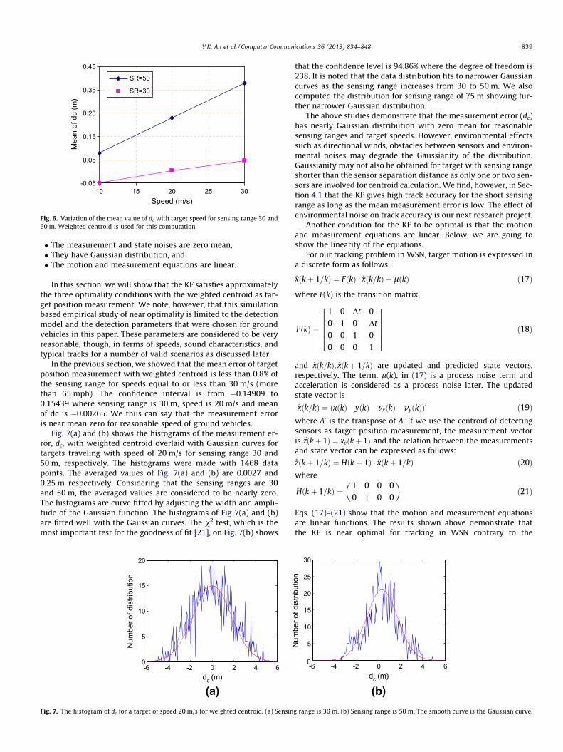
It is an expected result as the truth target position is far aheadfrom the geometric center for the high speed due to Doppler effect.However, the implication of the result needs to be addressed. Thepower law detection model of Eq. (1), which is equivalent to targetposition measurement with geometric centroid, will have mea-surement bias if their trackers are used in real world for targetspeed >10 m/s. The results also show that the measurement biasis unavoidable even for weighted centroid for target speed>50 m/s. But as most of ground vehicles have speed less than50 m/s we may say that the measurement is almost unbiased withthe weighted centroid as shown in Fig. 6. Fig. 6 shows the timeaverage of detection error using weighted centroid vs. target speedfor sensing range 50 and 30 m. The mean of dc varies from 0.09 to0.4 for sensing range of 50 m and from 0.049 to 0.045 for sensingrange of 30 m as target speed varies from 10 to 30 m/s. Withinthe speed range, the maximum mean value is less than 0.8% and0.17% of the sensing range of 50 and 30 m respectively. The studyshows that within a reasonable target speed, the mean of dc is nearzero for various target sensing ranges.

3.3. Near optimality of Kalman Filter with the weighted centroid

KF becomes optimal filter if the following three conditions aresatisfied [10,20];

-6

-3

0

3

6

9

12

0 10 20 30 40Time (sec)

dc (m

)

(b)target speed of 50 m/s. (a) Weighted centroid, (b) Geometric centroid.

-0.05

0.05

0.15

0.25

0.35

0.45

10 15 20 25 30Speed (m/s)

Mea

n of

dc

(m)

SR=50

SR=30

Fig. 6. Variation of the mean value of dc with target speed for sensing range 30 and50 m. Weighted centroid is used for this computation.


� The measurement and state noises are zero mean,� They have Gaussian distribution, and� The motion and measurement equations are linear.

In this section, we will show that the KF satisfies approximatelythe three optimality conditions with the weighted centroid as tar-get position measurement. We note, however, that this simulationbased empirical study of near optimality is limited to the detectionmodel and the detection parameters that were chosen for groundvehicles in this paper. These parameters are considered to be veryreasonable, though, in terms of speeds, sound characteristics, andtypical tracks for a number of valid scenarios as discussed later.

In the previous section, we showed that the mean error of targetposition measurement with weighted centroid is less than 0.8% ofthe sensing range for speeds equal to or less than 30 m/s (morethan 65 mph). The confidence interval is from �0.14909 to0.15439 where sensing range is 30 m, speed is 20 m/s and meanof dc is �0.00265. We thus can say that the measurement erroris near mean zero for reasonable speed of ground vehicles.

Fig. 7(a) and (b) shows the histograms of the measurement er-ror, dc, with weighted centroid overlaid with Gaussian curves fortargets traveling with speed of 20 m/s for sensing range 30 and50 m, respectively. The histograms were made with 1468 datapoints. The averaged values of Fig. 7(a) and (b) are 0.0027 and0.25 m respectively. Considering that the sensing ranges are 30and 50 m, the averaged values are considered to be nearly zero.The histograms are curve fitted by adjusting the width and ampli-tude of the Gaussian function. The histograms of Fig 7(a) and (b)are fitted well with the Gaussian curves. The v2 test, which is themost important test for the goodness of fit [21], on Fig. 7(b) shows

-6 -4 -2 0 2 4 60

5

10

15

20

dc (m)

Num

ber o

f dis

tribu

tion

(a)Fig. 7. The histogram of dc for a target of speed 20 m/s for weighted centroid. (a) Sensin

that the confidence level is 94.86% where the degree of freedom is238. It is noted that the data distribution fits to narrower Gaussiancurves as the sensing range increases from 30 to 50 m. We alsocomputed the distribution for sensing range of 75 m showing fur-ther narrower Gaussian distribution.

The above studies demonstrate that the measurement error (dc)has nearly Gaussian distribution with zero mean for reasonablesensing ranges and target speeds. However, environmental effectssuch as directional winds, obstacles between sensors and environ-mental noises may degrade the Gaussianity of the distribution.Gaussianity may not also be obtained for target with sensing rangeshorter than the sensor separation distance as only one or two sen-sors are involved for centroid calculation. We find, however, in Sec-tion 4.1 that the KF gives high track accuracy for the short sensingrange as long as the mean measurement error is low. The effect ofenvironmental noise on track accuracy is our next research project.

Another condition for the KF to be optimal is that the motionand measurement equations are linear. Below, we are going toshow the linearity of the equations.

For our tracking problem in WSN, target motion is expressed ina discrete form as follows.

xðkþ 1=kÞ ¼ FðkÞ � xðk=kÞ þ lðkÞ ð17Þ

where F(k) is the transition matrix,

FðkÞ ¼

1 0 Dt 00 1 0 Dt

0 0 1 00 0 0 1

26664

37775 ð18Þ

and xðk=kÞ; xðkþ 1=kÞ are updated and predicted state vectors,respectively. The term, l(k), in (17) is a process noise term andacceleration is considered as a process noise later. The updatedstate vector is

xðk=kÞ ¼ ðxðkÞ yðkÞ vxðkÞ vyðkÞÞ0 ð19Þwhere A0 is the transpose of A. If we use the centroid of detectingsensors as target position measurement, the measurement vectoris ~zðkþ 1Þ ¼~xcðkþ 1Þ and the relation between the measurementsand state vector can be expressed as follows:

zðkþ 1=kÞ ¼ Hðkþ 1Þ � xðkþ 1=kÞ ð20Þwhere

Hðkþ 1=kÞ ¼1 0 0 00 1 0 0

� �ð21Þ

Eqs. (17)–(21) show that the motion and measurement equationsare linear functions. The results shown above demonstrate thatthe KF is near optimal for tracking in WSN contrary to the

-6 -4 -2 0 2 4 60

5

10

15

20

25

30

Num

ber o

f dis

tribu

tion

dc (m)

(b)g range is 30 m. (b) Sensing range is 50 m. The smooth curve is the Gaussian curve.

0 200 400 600 800 1000250

300

350

400

450

500

550

600

650

xtrajectory

ytra

ject

ory

Fig. 8. A trajectory of a target in acceleration with speed 20 m/s.


previous authors’ assertion, if weighted centroid is used for positionmeasurement.

For the completeness of this paper, we present the remaining KFequations below.

Pðkþ 1=kÞ ¼ FðkÞPðk=kÞFðkÞ0 þ QðkÞ ð22Þ

xðkþ 1=kþ 1Þ ¼ xðkþ 1=kÞ þWðkþ 1Þmðkþ 1Þ ð23Þ

Pðkþ 1=kþ 1Þ ¼ Pðkþ 1=kÞ �Wðkþ 1ÞSðkþ 1ÞWðkþ 1Þ0 ð24Þ

Sðkþ 1Þ ¼ Hðkþ 1ÞPðkþ 1=kÞHðkþ 1Þ0 þ Rðkþ 1Þ ð25Þ

Wðkþ 1Þ ¼ Pðkþ 1=kÞHðkþ 1Þ0Sðkþ 1Þ�1 ð26Þ

mðkþ 1Þ ¼ zðkþ 1Þ � Zðkþ 1=kÞ ð27Þ

Eq. (22) is the predicted state covariance with Q(k) being the covari-ance matrix of the process noise, l(k) of Eq. (17). Eqs. (23) and (24)are the updated state vector and updated state covariance matrix,S(k + 1) is the sum of measurement error and state error covariance,W(k + 1) is the Kalman gain, (k + 1) is the innovation or measure-ment residual, and R(k + 1) is the measurement error covariance.

The initializations of the state vector, state covariance, and mea-surement error covariance are determined empirically after runningthe tracker with numerous realistic parameters. The empiricaldetermination is a calibration process of the tracker. The initial xand y positions are selected from the x and y centroid computedat the start of track and initial x and y component of velocity areset to be 10 m/s as the velocity is reasonable for most of groundvehicles. The initializations of state (Eq. (28)) and measurementerror covariance matrix (Eq. (29)) are based on the simulationresults of various target speed and sensing ranges. The initial valuesof the process covariance Q(0) are determined knowing that Eq.17describes the linear target motion very accurately.

xð0Þ ¼ ðxc yc 10 10Þ ð28Þ

Pð0Þ ¼ diagð52 52 52 52Þ ð29Þ

Rð0Þ ¼ diagð52 52Þ ð30Þ

Qð0Þ ¼ diagð10�4 10�4 10�5 10�5Þ ð31Þ

Here, diag stands for diagonal elements of the matrix.

3.4. Tracking target in acceleration

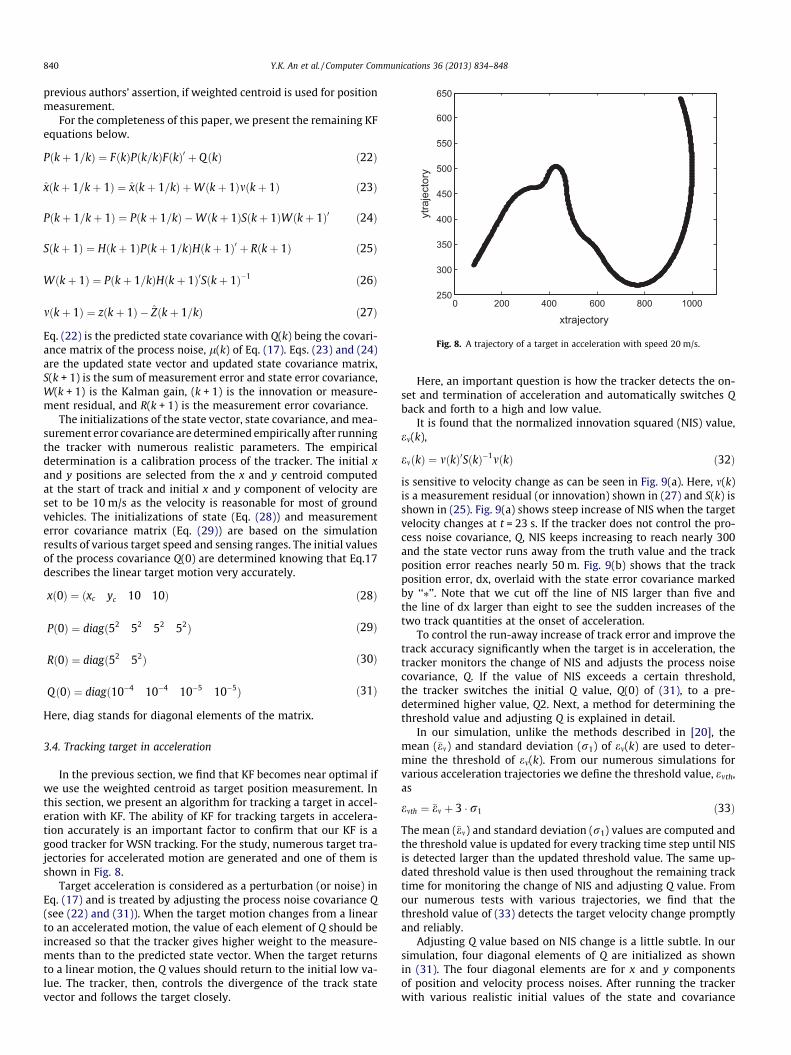
In the previous section, we find that KF becomes near optimal ifwe use the weighted centroid as target position measurement. Inthis section, we present an algorithm for tracking a target in accel-eration with KF. The ability of KF for tracking targets in accelera-tion accurately is an important factor to confirm that our KF is agood tracker for WSN tracking. For the study, numerous target tra-jectories for accelerated motion are generated and one of them isshown in Fig. 8.

Target acceleration is considered as a perturbation (or noise) inEq. (17) and is treated by adjusting the process noise covariance Q(see (22) and (31)). When the target motion changes from a linearto an accelerated motion, the value of each element of Q should beincreased so that the tracker gives higher weight to the measure-ments than to the predicted state vector. When the target returnsto a linear motion, the Q values should return to the initial low va-lue. The tracker, then, controls the divergence of the track statevector and follows the target closely.

Here, an important question is how the tracker detects the on-set and termination of acceleration and automatically switches Qback and forth to a high and low value.

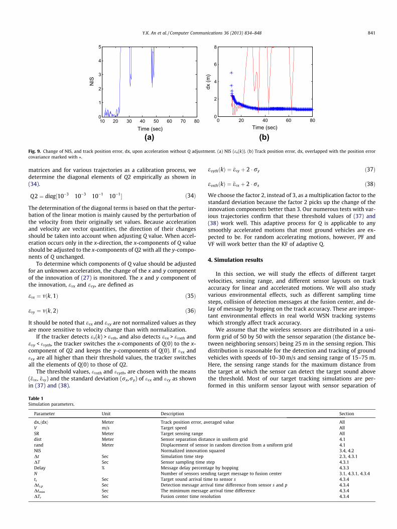
It is found that the normalized innovation squared (NIS) value,em(k),

emðkÞ ¼ mðkÞ0SðkÞ�1mðkÞ ð32Þ

is sensitive to velocity change as can be seen in Fig. 9(a). Here, m(k)is a measurement residual (or innovation) shown in (27) and S(k) isshown in (25). Fig. 9(a) shows steep increase of NIS when the targetvelocity changes at t = 23 s. If the tracker does not control the pro-cess noise covariance, Q, NIS keeps increasing to reach nearly 300and the state vector runs away from the truth value and the trackposition error reaches nearly 50 m. Fig. 9(b) shows that the trackposition error, dx, overlaid with the state error covariance markedby ‘‘⁄’’. Note that we cut off the line of NIS larger than five andthe line of dx larger than eight to see the sudden increases of thetwo track quantities at the onset of acceleration.

To control the run-away increase of track error and improve thetrack accuracy significantly when the target is in acceleration, thetracker monitors the change of NIS and adjusts the process noisecovariance, Q. If the value of NIS exceeds a certain threshold,the tracker switches the initial Q value, Q(0) of (31), to a pre-determined higher value, Q2. Next, a method for determining thethreshold value and adjusting Q is explained in detail.

In our simulation, unlike the methods described in [20], themean (�em) and standard deviation (r1) of em(k) are used to deter-mine the threshold of em(k). From our numerous simulations forvarious acceleration trajectories we define the threshold value, emth,as

emth ¼ �em þ 3 � r1 ð33Þ

The mean (�em) and standard deviation (r1) values are computed andthe threshold value is updated for every tracking time step until NISis detected larger than the updated threshold value. The same up-dated threshold value is then used throughout the remaining tracktime for monitoring the change of NIS and adjusting Q value. Fromour numerous tests with various trajectories, we find that thethreshold value of (33) detects the target velocity change promptlyand reliably.

Adjusting Q value based on NIS change is a little subtle. In oursimulation, four diagonal elements of Q are initialized as shownin (31). The four diagonal elements are for x and y componentsof position and velocity process noises. After running the trackerwith various realistic initial values of the state and covariance

10 20 30 40 50 60 70 800

1

2

3

4

5

0 20 40 60 800

2

4

6

8

Time (sec)

NIS

dx (m

)

Time (sec)

(a) (b)Fig. 9. Change of NIS, and track position error, dx, upon acceleration without Q adjustment. (a) NIS (ev(k)). (b) Track position error, dx, overlapped with the position errorcovariance marked with ⁄.


matrices and for various trajectories as a calibration process, wedetermine the diagonal elements of Q2 empirically as shown in(34).

Q2 ¼ diag½10�3 10�3 10�1 10�1� ð34Þ

The determination of the diagonal terms is based on that the pertur-bation of the linear motion is mainly caused by the perturbation ofthe velocity from their originally set values. Because accelerationand velocity are vector quantities, the direction of their changesshould be taken into account when adjusting Q value. When accel-eration occurs only in the x-direction, the x-components of Q valueshould be adjusted to the x-components of Q2 with all the y-compo-nents of Q unchanged.

To determine which components of Q value should be adjustedfor an unknown acceleration, the change of the x and y componentof the innovation of (27) is monitored. The x and y component ofthe innovation, emx and emy, are defined as

emx ¼ mðk;1Þ ð35Þ

emy ¼ mðk;2Þ ð36Þ

It should be noted that emx and emy are not normalized values as theyare more sensitive to velocity change than with normalization.

If the tracker detects em(k) > emth, and also detects emx > emxth andemy < emyth, the tracker switches the x-components of Q(0) to the x-component of Q2 and keeps the y-components of Q(0). If emx andemy are all higher than their threshold values, the tracker switchesall the elements of Q(0) to those of Q2.

The threshold values, emxth and emyth, are chosen with the means(�emx, �emy) and the standard deviation (rx,ry) of emx and emy as shownin (37) and (38).

Table 1Simulation parameters.

Parameter Unit Description

dx,hdxi Meter Track position error, avV m/s Target speedSR Meter Target sensing rangedist Meter Sensor separation distarand Meter Displacement of sensoNIS Normalized innovationDt Sec Simulation time stepDT Sec Sensor sampling timeDelay % Message delay percentN Number of sensors sents Sec Target sound arrival timDts,p Sec Detection message arriDtmin Sec The minimum messageDTr Sec Fusion center time res

evythðkÞ ¼ �emy þ 2 � ry ð37Þ

evxthðkÞ ¼ �emx þ 2 � rx ð38Þ

We choose the factor 2, instead of 3, as a multiplication factor to thestandard deviation because the factor 2 picks up the change of theinnovation components better than 3. Our numerous tests with var-ious trajectories confirm that these threshold values of (37) and(38) work well. This adaptive process for Q is applicable to anysmoothly accelerated motions that most ground vehicles are ex-pected to be. For random accelerating motions, however, PF andVF will work better than the KF of adaptive Q.

4. Simulation results

In this section, we will study the effects of different targetvelocities, sensing range, and different sensor layouts on trackaccuracy for linear and accelerated motions. We will also studyvarious environmental effects, such as different sampling timesteps, collision of detection messages at the fusion center, and de-lay of message by hopping on the track accuracy. These are impor-tant environmental effects in real world WSN tracking systemswhich strongly affect track accuracy.

We assume that the wireless sensors are distributed in a uni-form grid of 50 by 50 with the sensor separation (the distance be-tween neighboring sensors) being 25 m in the sensing region. Thisdistribution is reasonable for the detection and tracking of groundvehicles with speeds of 10–30 m/s and sensing range of 15–75 m.Here, the sensing range stands for the maximum distance fromthe target at which the sensor can detect the target sound abovethe threshold. Most of our target tracking simulations are per-formed in this uniform sensor layout with sensor separation of

Section

eraged value AllAllAll

nce in uniform grid 4.1r in random direction from a uniform grid 4.1

squared 3.4, 4.22.3, 4.3.1

step 4.3.1age by hopping 4.3.3ding target message to fusion center 3.1, 4.3.1, 4.3.4

e to sensor s 4.3.4val time difference from sensor s and p 4.3.4

arrival time difference 4.3.4olution 4.3.4

dx (m

)

14

10

6

2

0 5 10 15 20 25 30 35 0 5 10 15 20 25 30 35

dx (m

)

14

10

6

2

Time (Sec)

(a)Time (Sec)

(b)Fig. 10. Track position error with speed V = 50 m/s. (a) Geometric centroid. (b) Weighted centroid. Sensing range is 50 m for both cases. The state position error of thin line isplotted with the position state covariance of ⁄.


25 m. We also simulate target tracking in different sensor layouts;uniform grids with different sensor separations (20, 25, and 30 m)and random distribution of sensors. The simulation parametersused in this section is shown in Table 1.

4.1. Track accuracy for linear motions

In this section, track accuracy is studied for a target in linearmotion with speed of 50 and 10 m/s. The speed of 50 m/s is ratherhigh for ground vehicles but we take this number for comparisonpurpose. The centroids of detecting sensor positions computedwith and without weight are fed to the tracker as target positionmeasurements. As discussed in Section 3.3, weighted centroidcauses the KF near optimal by being closer to the true target posi-tion and leads to the relatively accurate target tracking.

Fig. 10 shows clearly the Doppler effect on the track accuracyfor a high speed target (50 m/s) with the sensing range 50 m. Notethat the sensing range is two times the distance between sensors.Fig. 10(a) is for the centroid without weight and (b) is for withweight. The position state error covariance (marked by ⁄) overlaysthe position track error. The figure shows that the track errorshown in Fig. 10(a) of geometric centroid is three times higher thanthat in Fig. 10(b) of weighted centroid and that the position stateerror covariance fits to the position error well for Fig. 10(b) butnot for Fig. 10(a). The high track error for Fig. 10(a) is caused bythe position measurement bias of the geometric centroid due tothe Doppler effect.

When the speed is low, the Doppler effect is reduced and thedifference between the weighted and geometric centroid de-creases. For the low speed (10 m/s), Fig 11(a) and (b) show that

20 30 40 50

6

5

4

3

2

1

0

Time (Sec)

(a)

dx (m

)

Fig. 11. Track position error with speed V = 10 m/s. (a) Geometric centroid. (b) Weightedpeak is plotted with the position state covariance.

the tracking error for geometric centroid is about 1.5 times higherthan for weighted centroid and the position error covariances fit tothe track error well for both cases. The Doppler effects are clearlyreflected for high and low speed targets in the tracking resultsabove.

Next, we are going to study the effects of different velocities andsensing ranges on the track accuracy. For the study of differentsensing ranges’ effect on track accuracy, we choose two sensingranges, 50 and 30 m in Fig 12(a) and compute the mean track posi-tion error, hdxi, for the speeds of 10–50 m/s.

The figure shows that as the speed becomes faster, the meantrack error becomes larger for both of the sensing ranges but theerror increase rate is higher for larger sensing range. Fig 12(b)shows position track error for target speed of 20 m/s and varioussensing ranges of 15–75 m. Note that the distance between neigh-boring sensors is 25 m and the sensing range of 15 m is muchshorter than the sensor distance. In the previous section, we men-tioned that the measurement error distribution is not near Gauss-ian for sensing range shorter than the distance between sensors.However, Fig. 12(b) shows that the track accuracy is very goodfor the sensing ranges shorter than the sensor distance. The resultsmay be understood with Fig. 12(c) which shows the mean mea-surement error vs. sensing range. For sensing ranges equal or lessthan 30 m, the mean measurement error is much lower than0.1 m but the error increases to 0.38 and 0.6 m as the sensing rangeincrease to 50 and 75 m. Fig. 12(b) and (c) imply that as long as themean measurement error is near zero, the track accuracy is stillgood even if the error distribution is off the Gaussian.

The results shown above are for a sensor layout in a uniformgrid with 25 m of sensor separation. Track accuracy may also be

20 30 40 50Time (Sec)

(b)

6

5

4

3

2

1

0

dx (m

)

centroid. Sensing range is 50 m for both cases. The state position error with multiple

00.20.40.60.8

11.21.4

0 20 40 60

<dx>

(m)

Velocity (m/s)

SR=50SR=30

0

0.1

0.2

0.3

0.4

0.5

0.6

0.7

0 20 40 60 80

<dx>

(m)

SR (m)

0

0.1

0.2

0.3

0.4

0.5

0.6

0.7

0 20 40 60 80

<dc>

(m)

SR (m)(a) (b) (c)

Fig. 12. (a) Averaged track position error, hdxi, in meter vs. target speed for sensing ranges 50 and 30 m. (b) Averaged track position error, hdxi, vs. sensing range (SR) fortarget speed 20 m/s. (c) Measurement error vs. sensing range (SR).

(a) (b) (c)Fig. 13. Three different sensor layouts. (a) Sensors are distributed in a uniform grid with 25 m of sensor separation. (b) Sensors are shifted from the uniform grid by 5 m inrandom directions. (c) Sensors are shifted from the uniform grid by 10 m in random directions. The sensors designated with ⁄ in red are the sensors that detect target soundabove the threshold. (For interpretation of the references to color in this figure legend, the reader is referred to the web version of this article.)


affected by different sensor separations in uniform grids and byrandom layouts of the sensors. We have studied the track accuracyfor sensors in a uniform grid with sensor separations of 20, 25, and30 m respectively and for three different sensor layouts as shownin Fig. 13. Fig. 13(a) is a uniform grid with sensor separation of25 m and Fig. 13(b) and (c) are random distributions of sensorsgenerated by shifting each sensor by 5 and 10 m respectively fromthe uniform grid in random directions.

Fig. 14(a) shows the mean position track error vs. target speedfor sensors in uniform grids with sensor separation 20, 25, and30 m. The target sensing range is set to be 40 m. For target velocitylower than 30 m/s, higher sensor separation gives higher track er-ror as the measurement error increases with higher sensor dis-tance. For target speed 30 m/s or higher, the track error forsensor separation of 30 m is slightly lower than the track errorfor sensor separation of 25 m showing intricate coupling betweenDoppler effect and higher sensor distance. Fig. 14(b) shows trackerror vs. target speed for the three different sensor layouts shownin Fig. 13. The figure shows that track error increases as the ran-dom shift increases from zero to 5 and10 m for target velocity lessthan 30 m/s. The Doppler effect on track error appears for targetvelocity P30 m/s for the random layouts. This study shows thatthe track accuracy is within a comparable range for various sensordensity and layouts.

4.2. Track accuracy for accelerated motions

Fig. 15 shows the result of controlling Q when the targetswitches back and forth between linear and accelerated motionsas shown by the trajectory of Fig. 8. Fig. 15(a) shows NIS changeand Fig. 15(b) shows drastic improvement of track accuracy whenQ value is adjusted based on the change of NIS as explained above.

Fig. 16 shows the track results for target sensing ranges of 30and 50 m with speed of 20 m/s. Here, we fix the sensor samplingtime to be 0.1 s and change the track time step and compute theaveraged position error for the target trajectory described inFig. 8. The averaged errors generally increase with increased track-ing time step and are higher than for the linear trajectory. The fig-ure shows that the sensing range of 50 m gives a little higher trackerror than the sensing range of 30 m. The result shows that theaccuracy of our KF compares favorably with other trackers thathave higher computational complexity for targets in acceleration.

4.3. Environmental effects

The uniqueness of our realistic detection model enables us tostudy the following environmental effects on the target tracking.We will show that the track accuracy is sensitive to these environ-mental effects.

4.3.1. Different sampling time stepsAs the sensors in WSN have limited power and communication

resources, it is desirable for each sensor to have longer samplingtime step for sending detection message to the fusion center aslong as track accuracy is not degraded. However, we have foundthat the increase of sampling time step gives an adverse effect onthe track accuracy and the effect is more serious than previousstudies indicated. Before going into details, we note that we usetwo different time steps; one is the simulation time step, Dt, withwhich target motion and sound propagation are simulated and theother is the sampling time step, DT. In our simulation, the simula-tion time step is fixed to be 0.005 s and the sampling time step var-ies from 0.1 to 1.0 s. The effect of different sampling time steps onthe target position measurement through the centroid computa-tion can be explained in a simple way as follows.

0

0.2

0.4

0.6

0.8

1

1.2

0 10 20 30 40 50

<dx>

(m)

Velocity (m/s)

dist=20dist=25dist=30

00.20.40.60.8

11.21.41.6

0 10 20 30 40 50

<dx>

(m)

Velocity (m/s)

rand=0rand=5rand=10

(a) (b)Fig. 14. Track position error vs. target velocity for different sensor layouts. (a) Track errors for sensors in uniform grids with distance between sensors (dist) 20, 25, and 30 m.(b) Track errors for three different sensor layouts shown in Fig. 13. The data label ‘‘rand’’ stands for sensor shift in meter in random direction from the uniform grid.

0 20 40 60 800

0.5

1

1.5

2

2.5

Time (sec)

NIS

0 20 40 60 800

2

4

6

8

Time (sec)

<dx>

(m)

(a) (b)Fig. 15. Change of NIS and track position error upon acceleration with Q adjustment. (a) NIS. (b) Track position error overlapped with the position error covariance markedwith ⁄.

0

0.5

1

1.5

2

2.5

3

3.5

0 0.2 0.4 0.6 0.8 1Time step (sec)

SR=50

SR=30

<dx>

(m)

Fig. 16. Averaged position error vs. different track time steps for targets of sensingrange 30 and 50 m in accelerated motion.


For simplicity, we assume that the sampling time is the same asthe detection message sending time, which means that a sensorsends a detection message to the fusion center as soon as it sam-ples a target sound higher than the threshold. For a given simula-tion time, t = t0, N0 number of sensors are assumed to be in thedetection region (the shaded area of Fig. 1(b)). If N1 out of the N0

number of sensors sent the detection messages to the fusion centerin t0 � DT < t < t0, those sensors are excluded for sampling at t = t0

and only N = N0–N1 number of sensors send the detection messageto the fusion center. When the sampling time step, DT, increases,N1 also increases so the number of sensors, N, that send the detec-

tion message at t = t0 decreases in average. When the fusion centercomputes the centroid based on the received message at t = t0 thecentroid does not represent an accurate target position measure-ment because of the missing messages.

Fig. 17 shows how different sampling times affect the numberof sensors which send detection message at a given simulationtime. Each of Fig 17(a)–(c) shows the number sensors for the sam-pling time step 0.1, 0.6, and 1.0 s, respectively, and each frameshows the sensors at five different times. The target is in the mid-dle of the sensors designated with a diamond. The target is movingdiagonally from the left lower corner to the right upper corner ofthe sensing area. As the time step, DT, is larger, the simulationshows that the number of message sending sensors decreases asmentioned above.

Fig. 18(a) and (b) show the number of sensors sending thedetection message to the fusion center every 0.1, 0.6, and 1.0 s dur-ing the target motion described above for target sensing range 75and 30 m respectively. For the sensing range 30 m and DT = 0.6and 1.0 s, sometimes there is no sensors which send detectionmessage to the fusion center. In this case, the tracking is skippeduntil at least one sensor sends the detection message to the fusioncenter. Thus, for short sensing range targets, the KF tracking timestep is variable. For sensing range of 15 m which is shorter thanthe distance between neighboring sensors, the number of sensorsthat send detection message can often be zero for several secondsof time interval.

Fig. 19 shows the dependence of the mean position track error,hdxi, on DT, for the sensing range of 15, 50, and 75 m. The figureshows that increasing DT gives higher track error because of theloss of the detection messages for centroid calculation. This study

0 200 400 600 800 1000 1200200

300400500600700

800900

100011001200

0 200 400 600 800 1000 1200200

300

400

500600

700

800900

1000

11001200

0 200 400 600 800 1000 1200200

300400

500600

700800

9001000

11001200

(a) (b) (c)Fig. 17. Each figure shows the sensors which send detection signal to the fusion center every DT s for five different simulation times. The target position is designated with adiamond in the middle of the sensors. (a) DT = 0.1 s, (b) DT = 0.6 s, (c) DT = 1.0 s. The target sensing range is 75 m and target velocity is 30 m/s.

0

5

10

15

20

25

30

35

40

Track time (sec)

Num

ber o

f sen

sors

(a)

0

1

2

3

4

5

6

7

0 20 40 60 0 20 40 60Track time (sec)

Num

ber o

f sen

sors

(b)

τΔ = 0.1

τΔ = 1.0

τΔ = 0.6

τΔ = 0.1

τΔ = 1.0

τΔ = 0.6

Fig. 18. The number of sensors that send detection message to fusion center every 0.1, 0.6, and 1.0 s for two different target sensing ranges. (a) Sensing range = 75 m, (b)Sensing range = 30 m.


shows that for accurate tracking, DT should be as short as possible,in other words, saving sensor energy requires significant sacrificeof track accuracy especially for sensing range 15 m. For sensingrange 15 m, the track error suddenly increases from 2.5 m to nearly8 m when DT increases from 0.8 to 1.0 s. Ahmed et al. [8] studiedthe track accuracy for different values of DT and found that besttracking results are obtained with 0.5 and 1.0 s of sampling time.The discrepancy of their result from ours may be attributed to their

0

2

4

6

8

10

0 0.2 0.4 0.6 0.8 1

<dx>

(m)

Sending time step (sec)

sr=75sr=50sr=15

Fig. 19. Dependence of track accuracy on the sampling time steps (detectionmessage sending time steps), DT, for various target sensing ranges (SR), 75, 50, and15 m. hdxi is the mean position track error in meter.

simple power law detection model and very low target speed of0.35 m/s.

4.3.2. Delay of detection message at the fusion center due to hoppingAs each of the wireless sensor nodes has short transmission

range, the detection message needs to be relayed to a remote fu-sion center by nearby sensors, in other words, the message signalmay require several hopping to reach the fusion center. The hop-ping delays the signal to reach the fusion center and the delay willaffect the tracking accuracy. In this section, we will study how themessage delay affects the track accuracy.

For the study, we select the delay time at the fusion center ran-domly in 0–0.1 s and choose the delayed messages randomly withthe ratios of 0%, 60%, and 100% of the detecting sensors at each sim-ulation time. The ratio of 100% means all the detecting sensors’messages are delayed and the ratio of 0% means none of the detect-ing sensors’ messages are delayed. We also assume that nearlyequal numbers of the delayed messages at each time step are filledwith the delayed messages in previous time steps. The delay timethat we choose for this study does not mean to reflect any real sen-sor delay time but for simulation purpose only. The accurate delaytime might be WSN systems dependent. Because of the mix of thedetection messages from current and previous simulation timesteps, the target position measurement estimate with the mes-sages will have a bias depending on the number of delayedmessages.

Fig. 20 shows the averaged position track error vs. target speedfor three different ratios of delayed messages. The figure shows

0

1

2

3

4

5

6

7

8

0 20 40 60

<dx>

(m)

Target Speed (m/s)

delay=100%

delay=60%

delay=0%

Fig. 20. The effect of detection message delay at the fusion center due to hoppingon averaged position track error for the delay ratio of 100%, 60% and 0%. The targetsensing range is 75 m and delay time is 0–0.1 s.


that the track errors increase with target speed and the rate of in-crease is higher for higher delay ratio. The track errors of 100% and60% of delay ratio are nearly 6 and 4 times higher than the trackerror of no delay. If the delay time is shorter than 0.1 s, the trackerrors will decrease below the levels shown in the figure. Thisstudy suggests that message delay by hopping can be fatal for trackaccuracy unless the delay time is reduced to much less than 0.1 sby having local fusion centers. Some authors [9,25,26] suggestedvarious ways of handling multiple hoppings or local fusion centersbut we do not consider them in detail in this paper.

4.3.3. Collision of detection messages at the fusion centerFor a target with sensing range of 75 m, there are 25–30 sensors

at each simulation time step that detect the target sound. Whenthese sensors send the detection message to the fusion center ondetection, there will be collisions between the messages dependingon the time resolution of the fusion center. In this section, we aregoing to study how different sensing ranges affect the collision andhow collisions affect the track accuracy.

For a given simulation time step, we have, for example, N num-ber of sensors that detect target sound. Because the distance be-tween the target and each of the sensors varies depending onsensor position, the detection time of each sensor is different bysensor position. We assume that each sensor sends a detectionmessage as soon as it detects the target sound and neglect messagedelay by hopping for simplicity. The detection time, then, can beconsidered as the message arrival time to the fusion center. We

0 0.2 0.4 0.6 0.8 1

x 10-3

0

10

20

30

min-time (sec)

dist

ribut

ion

(%)

SR=75m

0 0.2 0.40

10

20

30

min-tim

dist

ribut

ion

(%)

SR=50m

(a) (Fig. 21. The distribution of the minimum time difference, Dtmin, through the course of th(c) 30 m.

compute the time difference between the messages that arrivedat the fusion center and then find the minimum difference at eachsimulation time step as follows. For all the sensors that satisfy thetarget sound detection conditions shown by (11) and (12), thesound arrival time to each sensor is calculated as

ts ¼ ds;j=Vc ðs ¼ 1;2; . . . ;NÞ ð39Þ

We, then, compute the arrival time differences between the detect-ing sensors and find the minimum value from the differences ateach simulation time step.

Dts;p ¼ jts � tpj ; ðs ¼ 1;2; . . . ;N � 1Þ and ðp ¼ sþ 1; . . . ;NÞ ð40Þ

Dtmin ¼minðDts;pÞ ð41Þ

If the time resolution of the fusion center, DTr, is lower than theminimum difference, Dtmin, the fusion center can process all themessages without missing any of them. But if DTr is larger thanDtmin, some of the messages will be lost. The minimum difference,Dtmin, fluctuates with simulation time in the range of 0–10�3 s asthe distance between the moving target and each of the detectingsensors varies with time. The distribution of Dtmin throughout thetarget track time varies depending on the size of sensing range asshown in Fig. 21.

Fig. 21(a)–(c) show the percentage distribution of Dtmin for tar-get speed 30 m/s and sensing range 75, 50, and 30 m respectively.The horizontal axis is for Dtmin and the vertical axis is for the per-centage distribution of Dtmin. We compute the percentage with to-tal about 360 samples. The average number of detecting sensors ateach simulation time is 28, 13, and 5 for sensing ranges 75, 50, and30 m respectively. The figure shows that 40% of the samples haveDtmin 6 5 � 10�5 s for sensing range 75 m. For sensing range of50 and 30 m, 28% and 78% of the samples have Dtmin P 10�3 srespectively. The results imply that if the time resolution of the fu-sion center, DTr, is 5 � 10�5 s, it can handle most of the messageswithout collisions for all the sensing ranges shown above.

The effect of the collision on the track accuracy is studied withthe following process. From Eqs. (40) and (41), we computethe time difference, Dts,p for a given detection message s and p. IfDts,p < DTr, then the message s is discarded, otherwise, the messageis kept to send it to the fusion center. This process continues for alls = 1,2, . . .,N � 1 and p = s + 1, . . .,N, and send all the messages thatsurvive from this selection process to fusion center.

Fig. 22 shows the effect of fusion center time resolution, DTr, onthe track accuracy for the three different sensing ranges. The hor-izontal axis is for different time resolutions and the vertical axis isfor mean track position error in meter. The figure shows that long-er sensing range gives higher track error for all time resolutions.The track result matches well with the prediction from Fig. 21 as

0.6 0.8 1x 10-3e (sec)

0 0.2 0.4 0.6 0.8 1x 10-3

0

20

40

60

80

min-time (sec)

dist

ribut

ion

(%)

SR=30m

b) (c)e target travel with the speed of 30 m/s. Sensing range (SR) is (a) 75 m, (b) 50 m, and

0

0.4

0.8

1.2

1.6

2

0.E+00 2.E-04 4.E-04 6.E-04 8.E-04 1.E-03

<dx>

(m)

Time resolution (sec)

SR=75SR=50SR=30

Fig. 22. The effect of fusion center time resolution, DTr, on track position error forsensing range 75, 50, and 30 m. Target speed is 30 m/s.


mentioned above showing that the time resolution of 5 � 10�5 scan handle all the collisions without degrading track accuracymuch.

Ahmed et al. [8] studied packet losses occurred in a real multi-hop network deployment due to channel contention, collisions,and queues overflows in the buffers. At this moment, it is unclearhow their experimental result of collision is compared with oursimulation result as we lack detailed knowledge of their experi-ments. Comprehensive simulation studies for the effects of thesepacket losses on track accuracy with realistic parameters areimportant work to perform in the future.

5. Comparison with previous work

The main difference between our work and the previous studiesmentioned in the introduction is that we have developed a morerealistic model for target sound propagation and detection that ac-counts for the Doppler effect. Previous studies used a power law forsound power propagation and detection model in their trackersneglecting the Doppler effect. As the power law detection modelsin their trackers are susceptible to the mismatch with the soundpower detection by the sensors deployed in the field, we expectthat the track error by PF and VF of the previous studies may in-crease by factor of two or three higher than reported in their pa-pers when used in real world WSN.

Ahmed et al. [8] studied the track accuracy for different sensorsampling times and found that best tracking results are obtainedwith 0.5 and 1.0 s of sampling time. Our result in Section 4.3.2shows, however, that the maximum time step that gives reason-ably good tracking results is 0.2 s, above which the track accuracydeteriorates rapidly with increasing time steps. The discrepancybetween our result and the result of Ahmed et al. may be attributedto their simple detection model and their low target speed. Thiscomparison demonstrates the importance of using realistic detec-tion model and realistic target speed for the WSN tracking simula-tion. We have also studied the effects of message delay due tohopping, and message collisions on the track accuracy but noneof the previous work studied these environmental effects.

Any direct comparison of our track accuracy and computationalcomplexity with other trackers is beyond the scope of this paper asour KF tracker is integrated with our detection model while theprevious studies used a simple power law detection model. How-ever, Teng et al. [9] compared their VF results with the PF andSOI-KF results and found that the VF gives higher accuracy thanthe PF and SOI-KF results. The computation time of the VF is re-ported to be similar to that of the PF but is nearly 50 times higherthan the computing time of the SOI-KF. Ristic et al. [10] also com-

pared the track accuracy and computing time for tracking a reentryobject by the PF and extended KF (EKF) methods. They showed thetrack accuracy improvement by the PF method over EKF but the PFcomputing time was 100 times longer than EKF time. Consideringthat our KF is less complex than EKF and SOI-KF, these studies sug-gest that our KF is about 100 times faster than the PF and VF track-ers. For track accuracy, our position error of a target in accelerationis 1.2–3 m for sensing range 30 and 50 m (see Fig. 14) which iscompared well with the errors of 1.85 m for VF, 5.64 m for PF,and 11.01 m for SOI-KF [9]. We note that the comparison is tenta-tive as the target speed and sensing range are not explicitly speci-fied in [9] and the target trajectories used for both studies are notthe same.

6. Conclusion

The implementation requirements of WSN trackers in the realworld are low computing complexity with high track accuracyand robust tracking in real environments. The tracker is also re-quired to be verified and validated using simulations in which real-istic detection model and environmental effects are implemented.To satisfy the requirements of WSN, we have developed a realisticWSN detection algorithm from which the Doppler effect naturallyappears depending on target velocity. For a tracker of low comput-ing complexity, we use the KF with weighted centroid of detectingsensors as target position measurement. The weighted centroidmakes our tracker independent of detection models and becomesimpervious to the mismatch of detection between the trackerand the sensors deployed in the field. We also find that the KF be-comes near optimal filter with the weighted centroid for the detec-tion model and detection parameters used in this study.

The high computing speed and high track accuracy will makethe WSN tracking system inexpensive to implement in the realworld, which is one of crucial factors for WSN. With our detectionmodel and KF tracker, we plan to expand this study to multiple tar-gets tracking in noisy environments to verify the robustness of thetracker in real environments.

References

[1] K. Mechitov, S. Sundresh, Y. Kwon, G. Agha, Cooperative tracking with binarydetection sensor networks, Technical Report UIUCDCS-R-2003-2379,University of Illinois at Urbana-Champaign, September 2003.

[2] W. Kim, K. Mechitov, J. Choi, S. Ham, On target tracking with binary proximitysensors, in: Proc. IEEE Fourth Int’l Symp. Information Processing in SensorNetworks, Los Angeles, USA, April 2005, pp. 301–308.

[3] Z. Wang, E. Bulut, B. Szymanski, A distributed cooperative target tracking withbinary sensor networks, in: Proc. IEEE Int’l Conf. on Communications (ICC ‘08),Communication Workshop, Beijing, China, May 2008, pp. 306–310.

[4] Z. Wang, E. Bulut, B. Szymanski, Distributed target tracking with imperfectbinary sensor networks, in: Proc. IEEE Global Telecommunications Conference(Globecom ’08), New Orleans, USA, November 2008, pp. 1–5.

[5] A. Ribeiro, G.B. Giannakis, S.I. Roumeliotis, SOI-KF: distributed Kalman filteringwith low-cost communications using the sign of innovations, IEEETransactions on Signal Processing 54 (12) (December 2006) 4782–4795.

[6] P.M. Djuric, M. Vemula, M. Bugallo, Signal processing by particle filtering forbinary sensor networks, in: Proc. IEEE 11th Digital Signal Processing Workshopand IEEE Signal Processing Education Workshop, Taos Ski Valley, NM, USA,August 2004, pp. 263–267.

[7] P.M. Djuric, M. Vermula, M. Bugallo, Target tracking by particle filtering inbinary sensor networks, IEEE Transactions on Signal Processing 56 (6) (June2008) 2229–2238.

[8] N. Ahmed, M. Rutten, T. Bessell, S.S. Kanhere, N. Gordon, S. Jha, Detection andtracking using particle-filter-based wireless sensor networks, IEEETransactions on Mobile Computing 9 (9) (September 2010) 1332–1345.

[9] J. Teng, H. Snoussi, C. Richard, Decentralized variational filtering for targettracking in binary sensor networks, IEEE Transactions on Mobile Computing 9(10) (October 2010) 23.

[10] B. Ristic, S. Arulampalam, N. Gordon, Beyond the Kalman Filters for TrackingApplications, Artech House, 2004.

[11] N. Ahmed, Y. Dong, S. Kanhere, S. Jha, M. Rutten, T. Bessell, N. Gordon,Performance evaluation of a wireless sensor network based tracking system,


in: Proc. IEEE Fifth Int’l l Conf. Mobile Ad Hoc and Sensor Systems (MASS ’08),Atlanta, USA, October 2008, pp. 163–172.

[12] D. Li, K. Wong, Y. Hu, A. Sayeed, Detection, classification and tracking of targetsin distributed sensor networks, IEEE Signal Processing Magazine 19 (2) (March2002) 17–29.

[13] M.S. Arulampalam, S. Maskell, N. Gordon, T. Clapp, A tutorial on particle filtersfor online nonlinear/non-Gaussian Bayesian tracking, IEEE Transactions onSignal Processing 5 (2) (February 2002) 174–188.

[14] R. Brooks, P. Ramanathan, A.M. Sayeed, Distributed target classification andtracking in sensor networks, Proceedings of the IEEE 91 (8) (August 2003)1163–1171.

[15] A. Doucet, B. Vo, C. Andrieu, M. Davy, Particle filtering for multi-target trackingand sensor management, in: Proc. Fifth Int’l Conf. Information Fusion,Annapolis, vol. 1, USA, November 2002, pp. 474–481.

[16] W. Chen, J. Hou, L. Sha, Dynamic clustering for acoustic target tracking inwireless sensor networks, IEEE Transactions on Mobile Computing 3 (3) (July2004) 258–271.

[17] A. Arora, P. Dutta, S. Bapat, B. Kulathumani, H. Zhang, V. Naik, V. Mittal, H. Cao,M. Demirbas, M. Gonda, Y. Choi, H. Herman, S. Kulkarni, U. Arumugam, M.Nesterenko, A. Vora, M. Miyashita, A line in the sand: a wireless sensornetwork for target detection, classification, and tracking, Computer Networks46 (5) (December 2004) 605–634.

[18] D.S. Friedlander, S. Phoha, Semantic information fusion for coordinated signalprocessing in mobile sensor networks, International Journal of HighPerformance Computing Applications 16 (3) (August 2002) 235–241.

[19] W.R. Heinzelman, A. Chandrakasan, H. Balakrishnan, Energy-efficientcommunication protocol for wireless microsensor networks, in: Proc. ofthe Hawaii Int’l Conf. on Sys. Sci. vol. 2, Maui, Hawaii, USA, January 2000, pp. 10.

[20] Y. Bar-Shalom, X. Li, T. Kirubarajan, Estimation with Applications to Trackingand Navigation – Theory, Algorithms and Software, John Wiley & Sons, Inc.,New York, 2001.

[21] R.J. Barlow, Statistics, John Wiley & Sons, Inc., New York, 1989.[22] J.H. Kotecha, P.M. Djuric, Gaussian particle filtering, IEEE Transactions on

Signal Processing 51 (10) (October 2003) 2592–2601.[23] J.H. Kotecha, P.M. Djuric, Gaussian sum particle filtering, IEEE Transactions on

Signal Processing 51 (10) (October 2003) 2602–2612.[24] R. Olfati-Saber, Distributed Kalman filtering for sensor networks, in: Proc. of

the 46th IEEE Conf. on Decision and, Control, December 2007.[25] S. Pattem, S. Poduri, B. Krishnamachari, Energy-quality tradeoff for target

tracking in wireless sensor networks, in: Proc. Int’l Conf. InformationProcessing in Sensor Network, 2003, pp. 32–46.

[26] S. Singh, U. Madhow, E.M. Belding, Shaping throughput profiles in multihopwireless networks: a resource-biasing approach, IEEE Transactions on MobileComputing 11 (3) (March 2012).

[27] A. Athalye, V. Savic, M. Bolic, P.M. Djuric, Radio frequency identification systemfor accurate indoor localization, in: Proc. of IEEE Int. Conf. on Acoustic, Speechand Signal Proceeding (ICASSP), 2011.

[28] V. Savic, A. Athalye, M. Bolic, P.M. Djuric, Particle filtering for indoor RFID tagtracking, in: Proc. of IEEE Statistical Signal Processing Workshop (SSP), 2011.

[29] Z. Chen, L. Chen, M. Cetin, A.S. Willsky, An efficient message passing algorithmfor multi-target tracking, in: Proc. of 12th Int. Conf. on, Information Fusion,2009.

[30] M.R. Morelande, Joint data association using importance sampling, in: Proc. of12th Int. Conf. on, Information Fusion, 2009.

[31] A. Athalye, V. Savic, M. Bolic, P.M. Djuric, A novel semi-passive rfid system forindoor localization, IEEE Sensors Journal 13 (2) (2013) 528–537.

Doppler effect on target tracking in wireless sensor...

Documents

Transcript of Doppler effect on target tracking in wireless sensor...