Dooptionmarketscorrectlypricethe …yacine/comp.pdf ·...

*Corresponding author. Tel.: #1-609-258-4015; fax: #1-609-258-0719.E-mail address: [email protected] (Y. AmK t-Sahalia).

Journal of Econometrics 102 (2001) 67}110

Do option markets correctly price theprobabilities of movement of

the underlying asset?

Yacine AmK t-Sahalia��*, Yubo Wang�, Francis Yared�

�Department of Economics, Princeton University, Princeton, NJ 08544-1021, USA�Fixed Income Research, J.P. Morgan Securities Inc., New York, NY 10017, USA

�Lehman Brothers International (Europe), London EC 2M7HA, UK

Received 4 January 1999; received in revised form 21 August 2000; accepted 2 October 2000

Abstract

We answer this question by comparing te risk-neutral density estimated in completemarkets from cross-section of S&P 500 option prices to the risk-neutral density inferredfrom the time series density of the S&P 500 index. If investors are risk-averse, the latterdensity is di!erent from the actual density that could be inferred from the time series ofS&P 500 returns. Naturally, the observed asset returns do not follow the risk-neutraldynamics, which are therefore not directly observable. In contrast to the existingliterature, we avoid making any assumptions on investors' preferences, by comparing tworisk-adjusted densities, rather than a risk-adjusted density from option prices to anunadjusted density from index returns. Our only maintained hypothesis is a one-factorstructure for the S&P 500 returns. We propose a new method, based on an empiricalGirsanov's change of measure, to identify the risk-neutral density from the observedunadjusted index returns. We design four di!erent tests of the null hypothesis that theS&P 500 options are e$ciently priced given the S&P 500 index dynamics, and reject it.By adding a jump component to the index dynamics, we are able to partly reconcile thedi!erences between the index and option-implied risk-neutral densities, and proposea peso-problem interpretation of this evidence. � 2001 Elsevier Science S.A. All rightsreserved.

JEL classixcation: C14; G13

0304-4076/01/$ - see front matter � 2001 Elsevier Science S.A. All rights reserved.PII: S 0 3 0 4 - 4 0 7 6 ( 0 0 ) 0 0 0 9 1 - 9

�See Ross (1976), Banz and Miller (1978), Breeden and Litzenberger (1978) and Harrison andKreps (1979).

�See Cox and Ross (1976), Merton (1976), Jarrow and Rudd (1982), Bates (1991), Goldberger(1991), Longsta! (1995) and Bakshi et al. (1997).

�See Shimko (1993), Derman and Kani (1994), Dupire (1994), Rubinstein (1994), Stutzer (1996),Jackwerth and Rubinstein (1996), AmK t-Sahalia and Lo (1998) and Dumas et al. (1998).

Keywords: State-price densities; Risk-neutral densities; Density comparison; Arbitragerelationships; Girsanov's Theorem; Implied volatility smile; Jump risk; Peso problem

1. Introduction

Do investors rationally forecast future stock price distributions when theyprice options? Provided that markets are dynamically complete, arbitragearguments tie down option prices to the prices of primary assets. We maytherefore expect that option prices will accurately re#ect the risk implicit in thestochastic dynamics of their underlying assets } and nothing else. Is this the caseempirically, at least within the framework of a given class of models?

An arbitrage-free option pricing model can be reduced to the speci"cation ofa density function assigning probabilities to the various possible values of theunderlying asset price at the option's expiration. This density function is namedthe state-price density (SPD), due to its intimate relationship to the prices ofArrow}Debreu contingent claims.� A number of econometric methods are nowavailable to infer SPDs from option prices. These methods deliver SPD esti-mates which either relax the Black}Scholes (1973) and Merton (1973) log-normalassumption in speci"c directions,� or explicitly incorporate the deviations fromthe Black}Scholes model when estimating the option-implied SPD and pricingother derivative securities.� One of the main attractions of the latter methods isthat they produce direct estimates of the Arrow}Debreu state prices implicit inthe market prices of options. Their main drawback is that they empiricallyignore the evidence contained in the observed time series dynamics of theunderlying asset } which, in theory, should indeed be redundant information.

The goal of this paper is to examine whether the information contained in thecross-sectional option prices and the information contained in the time series ofunderlying asset values are empirically consistent with each other, i.e., whetheroption prices are rationally determined, under the maintained hypothesis thatthe only source of risk in the economy is the stochastic nature of the asset price.More concretely, does the S&P 500 option market correctly price the S&P 500index risk? It is certainly tempting to answer this question simply by comparingfeatures of the SPD implied by S&P 500 option prices to features of theobservable time series of the underlying asset price.

68 Y. An(t-Sahalia et al. / Journal of Econometrics 102 (2001) 67}110

�See Chiras and Manaster (1978), Schmalensee and Trippi (1978), Macbeth and Merville (1979),Rubinstein (1985), Day and Lewis (1988, 1990), Engle and Mustafa (1992), Canina and Figlewski(1993), Lamoureux and Lastrapes (1993), and for a study of the e!ect of institutional features onthese comparisons Harvey and Whaley (1992).

�See AmK t-Sahalia and Lo (2000) and Jackwerth (2000).�See for example Mehra and Prescott (1985) and Cochrane and Hausen (1992).

In fact, previous studies in the literature have always compared the observedoption data to the observed underlying returns data, i.e., a risk-neutral density toan actual density. Naturally, in the case where all the Black}Scholes assumptionshold, the comparison between the option-implied and the asset-implied SPDs,both log-normal with the same mean, reduces to a comparison of impliedvolatilities, assumed common across the cross-section of options, to the index'stime series realized volatility over the life of the option.� More generally, thewell-documented presence in option prices of an &implied volatility smile', wherebyout-of-the-money put options are more expensive than at-the-money options,directly translate into a negatively skewed option-implied SPD. At the same time,there is evidence in the S&P 500 time series of time-varying volatility, generallynegatively correlated with the index changes, as well as jumps; both of these e!ectscan give rise to a negatively skewed SPD. We argue in this paper that no conclu-sions regarding the rationality of option prices should be drawn from puttingthese two pieces of evidence together. The distribution of the underlying assetvalues that can be inferred from its observed time series, and the SPD implied byoption prices, are not comparable without assumptions on investors' preferences.

In fact, it is possible to use the exact same data to determine the representativepreferences that are implicit in the joint observations on option and underlyingasset prices.� In other words, the extra degree of freedom introduced by prefer-ences can &reconcile' any set of option prices with the observed time seriesdynamics of the underlying asset (up to suitable restrictions). Thus it is alwayspossible to conclude that the options are rationally priced from a comparison ofthe option-implied SPD and the actual density of index returns, when prefer-ences (albeit strange ones) can be found that legitimize the observed optionprices. Yet very little is known about aggregate investors' preferences } evenwithin the class of isoelastic utility functions, there is wide disagreement in theliterature regarding what constitutes a reasonable value of the coe$cient ofrelative risk aversion: is the coe$cient of relative risk aversion equal to 5 or250?� Therefore there is no reason a priori to compare the dynamics of theunderlying asset that are implied by the option data to the dynamics implied bythe actual time series, unless for some reason one holds a strong prior view onpreferences. Consequently, the combination of the facts that the observed S&P500 returns are negatively skewed and that there exists a persistent impliedvolatility smile, cannot be used as evidence either in favor or against therationality of option prices.

Y. An(t-Sahalia et al. / Journal of Econometrics 102 (2001) 67}110 69

In fact, the two SPDs need not even belong to the same parametric family,meaning that comparisons of their variances alone, as would be appropriateunder the Black}Scholes assumptions, can lead to type-II errors (if the varianceshappen to be equal but other features of the densities are distinct) and/or type-Ierrors (if the SPDs are in fact equal but the variance estimates are inconsistentdue to misspeci"cation of the assumed parametric form). For instance, Lo andWang (1995) give an example of misspeci"ed variance estimates in a simplercontext. The di$culty at this point is that we do not observe the data that wouldbe needed to infer directly the time-series SPD, since we only observe the actualrealized values of the S&P 500, not its risk-neutral values.

The main novelty in this paper is to show that it is nevertheless possible to usethe observed asset prices to infer indirectly the time-series SPD that should beequal to the option-implied cross-sectional SPD. We rely on Girsanov's charac-terization of the change of measure from the actual density to the SPD: thedi!usion function of the asset's dynamics is identical under both measures, onlythe drift needs to be adjusted. This fact is of course not surprising froma theoretical point of view, but had not been exploited empirically. Our econo-metric strategy is to start by estimating the di!usion function from the observedS&P 500 index returns. Then by Girsanov's Theorem, this is the same di!usionfunction as the di!usion function of the risk-neutral S&P 500 returns. Whatremains to be done is to adjust the drift to re#ect the risk-neutral rate of return.Fortunately, it turns out that this drift can be inferred from the observed pricesof market-traded instruments. The price of an S&P 500 futures contract givesthe risk-neutral expected value of the S&P 500 (cash) index at the contract'sexpiration. From these we obtain the risk-neutral drift rate of the S&P 500index. Having fully characterized the S&P 500 risk-neutral dynamics, it is theneasy to obtain the corresponding time-series SPD. We already discussed how toextract cross-sectional SPDs from option prices. By comparing the two SPDs} cross-sectional and time-series } our methodology allows us to assess whetheroptions are priced rationally, without making assumptions about, or having toestimate, the representative preferences that are embodied in the market pricesof options.

We examine, using every option traded on the S&P 500 index between April1986 and December 1994, whether the rationality condition that the two SPDsbe equal holds empirically. Because we construct an exactly identi"ed systemwith separate identi"cation of the cross-sectional and time-series SPDs, theequality between the two SPDs becomes an over-identifying restriction. As such,that restriction is testable. Our approach can be contrasted to the situationwhere the option-implied SPD is compared to the actual distribution implied bythe time-series of asset values: such a system can only be identi"ed throughassumptions on preferences. In that case, no implications for market e$ciencyare left to be tested since all the information contained in the data has alreadybeen exploited just to construct the estimators. To obtain over-identifying


�Of course, it might be di$cult to justify in practice why option markets enjoy such large tradingvolumes if they truly were redundant assets. Our approach shares this limitation with the entireliterature that relies on market completeness to tie down the prices of di!erent assets.

restrictions, even more stringent restrictions must be imposed on preferences,which opens the door to a potentially severe joint hypothesis problem.

In addition to escaping the need to specify preferences, we also wish to avoid asecond type of joint hypothesis problem: when we compare the two SPDs, we makeas few assumptions as possible on the cross-section of options and the dynamics ofthe underlying asset. For that reason, we rely on nonparametric estimates (seeAmK t-Sahalia (1996) for a di!erent nonparametric approach to derivative pricing).Our test for rationality is therefore robust to the biases arising from the potentialmisspeci"cation of the option pricing model, the data-generating process for theasset values, and the speci"cation of investors' preferences. In e!ect, our onlymaintained assumption is that markets are dynamically complete,�with the aggreg-ate risk solely driven by the variations in the S&P 500 index.

We "nd empirically that the option-implied SPDs exhibit systematic excessiveskewness and kurtosis with respect to the index-implied SPDs and reject the nullhypothesis that the S&P 500 options can be e$ciently priced within the limitedcontext of a univariate speci"cation with no jumps. This is not just restating thatthe option data exhibit an implied volatility smile, which is of course well-knownby now. Instead this demonstrates that the implied volatility smile is incompat-ible with the dynamics of the S&P 500 returns } as captured by a univariatedi!usion } independently of investors' preferences. We then design out-of-sample trading schemes to exploit the SPD di!erences and show that theycapture superior pro"ts, due to the irrationality of option prices (at least duringthe period under consideration). We also document that the high Sharpe ratiosachieved by these trading schemes demand excessive variation in investors'marginal utilities, in the sense of Hansen and Jagannathan (1991).

In a sense, we have taken the univariate speci"cation as far as it could go bybeing #exible in every possible dimension (nonparametric on the speci"cation ofthe dynamic process, no assumptions whatsoever on representative preferences).The "rst main conclusion of our paper is that this model, even pushed to its most#exible limits, simply cannot explain the joint time series dynamics of S&P 500returns and cross-sectional properties of S&P 500 option prices. Moving awayfrom the restrictive nature of the univariate di!usion speci"cation, we are able topartly reconcile the di!erences between the index and option implied SPDs byadding a jump component to the index dynamics. We propose a peso-probleminterpretation of this evidence: cross-sectional option prices capture a premiumas compensation for the risk of a market crash, but actual realizations of thatjump are too infrequent to be consistently observed and re#ected in estimatesdrawn from the time series of asset returns. The prediction of this model is thattime series SPD estimates should be insu$ciently skewed and leptokurtic


See the conclusion for a discussion of what the over-identifying restrictions would be in this case.

relative to their cross-sectional counterparts, which is exactly what we foundempirically. In future work, we intend to incorporate stochastic volatility inaddition to jumps and test the ability of that broader speci"cation to fullyreconcile the joint observations on option and asset returns.

The paper is organized as follows. In Section 2 we present a brief review of theno-arbitrage paradigm, propose an estimation strategy for the cross-sectionaland time-series SPDs and construct a statistical test of the null hypothesis thatthe option-implied and index-implied SPDs are identical. We apply ourestimators to the S&P 500 options and index prices in Section 3. We concludein Section 4. Technical assumptions and results are in the Appendix.

2. Cross-sectional vs. time-series SPDs

2.1. Implications of no-arbitrage

Suppose that the uncertainty in the economy is driven by the stochastic valuesS�of an underlying asset at a future date ¹. There exists a riskless cash account

which can be used to borrow and lend without restrictions between dates t and¹"t#� at the instantaneous rate of return r

�� . During that period, the assetpays dividends continuously at rate �

�� . For simplicity, we take r�� and �

�� to benonstochastic. When markets are frictionless, a path-independent derivativesecurity with payo! �(S

�) at ¹ can be perfectly replicated by a dynamic trading

strategy involving the asset and a riskless cash account, i.e., the derivative isa redundant asset which can be priced by arbitrage.

In order to rule out arbitrage opportunities among the asset, the derivativeand the cash account, Harrison and Kreps (1979) showed that the pricingoperator mapping payo!s at date ¹ into prices at date t must be linear,continuous and strictly positive. The Riesz representation theorem then charac-terizes the derivative price as an integral, or expectation operator, applied to thederivative's payo! function. The SPD is the density function fH

�(S

�, S

�, �, r

�� , ��)to be used in the expectation, i.e.:

e��

�(S�) fH

�(S

�, S

�, �, r

�� , �� ) dS�(2.1)

is the price of a European-style derivative security with a single liquidatingpayo! �(S

�).

If we are willing to be more speci"c about the nature of the uncertainty in S�,

we can further characterize the SPD. Suppose that the vector S of n�asset prices


� In that case, the system of asset prices S in (2.2) supports an SPD if and only if the system oflinear equations �(S

�) ) �

�"�(S

�) admits at every instant a solution �

�such that

E�exp� �� ) �� d�/2��(R,

<�exp�!�� d=�!��

�� )�� d�/2��(R.

In the presence of an SPD, markets are complete if and only if rank �(S�)"n

�almost everywhere.

follows Ito( di!usions driven by n�independent Brownian motions=:

dS�"�(S

�) dt#�(S

�) d=

�(2.2)

with n�*n

�.� Consider the conditional density that is generated by the dynam-

ics

dSH�

"(r��!�

��)SH�dt#�(SH

�) d=H

�(2.3)

where=H is a Brownian motion. The transformation from= to=H and S toSH is an application of Girsanov's Theorem [see Harrison and Kreps (1979)].Let gH

�(S

�, S

�, �, r

�� ,�� ) denote this conditional density.Under the assumptions made, the two characterizations of the SPD are

identical, i.e., fH"gH. For example, in the Black}Scholes case wheren�"n

�"1 (r

��!�� ) is constant and �(SH

�)"� ) SH

�for a constant value of the

parameter �, the risk-neutral density is given by

fH��

(S�, S

�, �, r

�� , ��)"gH��

(S�, S

�, �, r

�� , ��)

"

1

S��2��

exp�![ln(��

��)!(r

��!��!��

�)�]�

2�� .(2.4)

If we denote by H the price of a European call option with maturity date ¹

and strike price X, i.e., (2.1) evaluated for the payo! function�(S

�)"max[S

�!X, 0], then Eq. (2.1) reduces to the well-known

Black}Scholes formula:

H��(F

�� ,X, �, r�� ;�)"e�� F

��(d�)!X�(d

�) (2.5)

where F��"S

�exp((r

��!��)�) is the forward price for delivery of the underly-

ing asset at date ¹ and

d�,

ln(F��/X)#(��/2)�

��, d

�,d

�!��. (2.6)


As we discussed in the Introduction, fH can only be compared to the condi-tional distribution gH of S

�given S

�implied by the dynamics (2.3), not to the

conditional distribution g implied by (2.2). This paper examines how well theequality fH"gH holds in the data, without making the Black}Scholes (1973)assumptions } or for that matter any alternative parametric restrictions } andstudies the deviations from equality that arise in the data, and their conse-quences. In Section 2.2, we will estimate the function fH from the cross-section ofoption prices. This step essentially consists in collecting the market prices Hof call options, and given that we know their payo! functions �, inverting or&de-convoluting' equation (2.1) to obtain fH.

In Section 2.3, we will then estimate the time-series SPD gH. Of course, therisk-neutral path of the index �SH

� is not observable. Our estimation method is

based on the fact, which follows from Girsanov's Theorem, that the instan-taneous volatility functions �( ) ) are identical under both the actual and risk-neutral dynamics. That is, the same function �( ) ) modi"es the Brownian shocksin both (2.2) and (2.3). Therefore, we can use the observable index values �S

� to

devise an estimator of �( ) ), and then use this estimate, in conjunction with thecharacterization of the drift �H(SH

�)"(r

��!�� )SH

�. The risk-neutral drift rate

(r��!�

�� ) is readily observable from the spot-forward parity relationship

r��!�

��"ln(F

��/S�)

�(2.7)

where both F�� and S

�are date-t market prices.

Throughout, we never need to observe the process �SH�, yet we are estimating

its conditional density gH, not the actual density g of the process �S�. We can

then proceed in Section 2.4 to examine whether our nonparametric estimators offH and gH are identical.

2.2. Cross-sectional inference: SPD inferred from option data

In order to estimate fH from option prices, we use the nonparametric methodof AmK t-Sahalia and Lo (1998). This method exploits an insight of Banz andMiller(1978) and Breeden and Litzenberger (1978). Building on Ross's (1976) funda-mental realization that options can be combined to create pure Arrow}Debreustate-contingent claims, Banz and Miller (1978) and Breeden and Litzenberger(1978) provide a strategy for obtaining an explicit expression for fH as a functionof H: fH is the future value of the second derivative of the call option pricingformula H with respect to the option's strike price X. This can be seen either bya direct calculation of the integral in (2.1), or more intuitively by forminga butter#y portfolio with three call options, and letting the interval between thestrike prices of these call options shrink to zero.

Based on this characterization, AmK t-Sahalia and Lo (1998) take the option-pricing formulaH to be an arbitrary nonlinear function of a pre-speci"ed vector


� Locally polynomial estimators (especially linear, p"1) are a better choice in general than theNadaraya}Watson estimator (p"0), especially for small sample sizes. In our empirical application,the sample sizes are large enough to alleviate the need to consider locally polynomial estimators. Seealso AmK t-Sahalia and Duarte (1999) for a local polynomial-based estimator that incorporates shaperestrictions (such as the monotonicity and convexity of the price function).

of option characteristics or &explanatory' variables, Z,[F�� ,X, �, r

��], and usekernel regression to construct a nonparametric estimate of the function H. TheestimatorHK can then be di!erentiated twice to produce an estimator of the SPD,according to fH

�( ) )"exp(r

��)��H( ) )/�X�. In practice, the dimension of thekernel regression can be reduced by using a semiparametric approach. Thed-dimensional vector of explanatory variables Z is partitioned into [ZI ,F

�� , r��]where ZI ,[X/F

�� , �] contains dI "2 regressors. Suppose that the call pricingfunction is given by the parametric Black}Scholes formula (2.5) except that theimplied volatility parameter for that option is a nonparametric function �(ZI ):

H(S�,X, �, r

�� , ��)"H��(F

�� ,X, �, r�� ; �(X/F

�� , �)). (2.8)

To estimate �(X/F�� , �), the Nadaraya}Watson kernel estimator� is given by

�( (X/F�� , �)"

��

k��

X/F��!X

�/F

�� h��

�k��!�

�h� ��

��

k��

(��

)k� (��

)(2.9)

where ��is the volatility implied by the option price H

�, and the univariate

kernel functions k��

and k� and the bandwidth parameters h��

and h� arechosen to optimize the asymptotic properties of the SPD estimator:

fK H�(S

�, S

�, �, r

�� , �� )"e�� HK (S

�,X, �, r

�� , ��)�X� �

��

(2.10)

where HK (S�,X,�, r

�� ,�� )"H��(F

�� ,X,�, r�� ,�� ; �( (X/F

�� ,�)).

2.3. Time-series inference: SPD inferred from returns data

Our time-series estimator of the SPD gH is based on inferring the conditionaldensity resulting from the risk-neutral evolution (2.3) of the asset price. Theessential di$culty is that we do observe the actual index values �S

�, rather than

the risk-neutral values �SH�. As we discussed above, we rely crucially on the

commonality of the di!usion function under both the actual and risk neutraldynamics of the asset price. We start in Section 2.3.1 by estimating the di!usionfunction ��( ) ) of the asset price dynamics using the actual price series �S

�, and

then proceed in Section 2.3.2 to use this estimate, in conjunction with the knownand observable drift of the risk-neutral dynamics, to estimate the time-seriesSPD gH.


2.3.1. Estimation of the asset's diwusion functionTo introduce as few unnecessary restrictions as possible on the behavior of the

process �S�, we select an estimator of the di!usion function ��( ) ) that does not

place restrictions on the drift function. We use Florens}Zmirou's (1993) non-parametric version of the minimum contrast estimators (hereafter FZ). FZprovides an unbiased nonparametric estimator for the di!usion coe$cient in theabove model. The frequency of the data is assumed to be high enough that thedrift � can be unknown and treated as a nuisance parameter. The estimateddi!usion at a point is the squared change of observations weighted by thecontribution to the local time of these observations. Without loss of generality,set t"0 and ¹"1, and assume that the process is sampled at the discrete datest�"i/N. The FZ estimator is based on a discrete approximation of the local

time in S of the di!usion function during [0, t],

¸�(S)"lim

��

1

2��

1�� du. (2.11)

¸�(S) is estimated consistently by

¸�(S)"

1

nh��

��

K�S�!S

h�� (2.12)

where [ ) ] denotes the integer part,K is a kernel function and h��

is a bandwidthparameter such that (Nh

��)� ln(N)P0 and Nh�

��P0 as the number of obser-

vations N tends to in"nity. When the trajectory of the di!usion visits the assetprice level S, the natural local estimator of the di!usion function at that level is

�( ��(S)"

��

K(��

)N�S��

!S��

��

��K(��

��)

(2.13)

which consistently estimates ��(S) as NPR, provided that Nh��

P0. More-over, if Nh�

��P0,

N��h��

�( ��(S)

��(S)!1� �

P ¸(S)�� ) Z (2.14)

where Z is a standard Normal variable independent of ¸(S).In order to assess the empirical performance of the estimator, we perform

Monte-Carlo simulations in conditions that approximate the real data. Wesimulate sample paths of the asset price process �S

� according to (2.2) with

a constant drift rate, �(S)"� ) S, and a di!usion function given by

�(S)" #�(S!S )#�(S!S

)�.


��The Milstein scheme is a strong Taylor discrete approximation of the continuous-time samplepath which converges strongly with an order 1.0. The traditionally-used Euler scheme convergessubstantially more slowly: its order of convergence is 0.5.

S is set to 400. The parameter represents the level of volatility, � the slope of

the volatility function and � its curvature at S . We consider various combina-

tions of , � and � and obtain a range of shapes for the di!usion function whichis capable of capturing the empirical features of the asset's dynamics.

To simulate the continuous-time sample paths, we generate three months ofdata using the Milstein scheme [see e.g., Kloeden and Platen (1992, Section10.3)] sampled every 5 minutes, assuming 8 hours of trading per day and 21trading days per month.�� We check whether the estimators do capture theshape of the di!usion by considering a #at, downward sloping and upwardsloping �( ) ) in our path simulations. Details on the simulations can be found inAppendix C [see Table 8 and Fig. 11]. The results show that �(

��( ) ) captures

very well the average level, slope and curvature of �( ) ). Since the estimator hasa local character, the di!usion function is estimated more precisely around theinitial level S

where most of the observations are recorded. The results of our

simulations also show that the estimator widely outperforms the standardmaximum-likelihood estimator, which assumes that the volatility parameter isconstant.

2.3.2. Estimation of the returns SPDOnce the volatility function �( ) ) of the index dynamics �S

� is estimated, we

can make use of Girsanov's characterization of the change of measure from theactual to the risk-neutral dynamics: the drift is set at the di!erence between theriskless rate and the dividend yield of the index, but the di!usion functionis unchanged. We can then recover the time-series SPD gH using one oftwo natural methods. We can either solve, for all possible values of S

�, the

Fokker}Planck partial di!erential equation

�gH

��#(r

��!��)

�gH

�S�

#

1

2�( �(S

�)��gH

�S�

"0 (2.15)

with the initial condition that gH(S,S, 0, r, �) is a Dirac mass at S, or computegH by Monte-Carlo integration.

In our empirical implementation below, we adopt the second method. Giventhe starting value of the index at the beginning of the period, we simulateM"10,000 sample paths of the estimated risk-neutral dynamics (2.3), where wehave replaced the di!usion function by its nonparametric estimate:

dSH�"(r

��!�� )SH

�dt#�(

��(SH

�) d=H

�(2.16)


and use the Milstein scheme. The end points at ¹ of these simulated paths arecollected as �S

��: m"1,2,M, and annualized three-month index log-returns

are calculated.We obtain the SPD gH of the future index values S�by construct-

ing a nonparametric kernel density estimator p( H�for the index continuously-

compounded log-returns u:

p( H�(u)"

1

Mh��

��

��

k��

u�

!u

h��

� (2.17)

where u�is the log-return recorded at the end of the mth sample path. From the

density of the continuously compounded log-returns we then have

Pr(S�

)S)"Pr(S�e�)S)"Pr(u)log(S/S

�))"�

��

�

pH�(u) du (2.18)

and can recover the price density gH corresponding to the return density pH as

gH�(S)"

��S

Pr(S�

)S)"pH�(ln(S/S

�))

S. (2.19)

As we show in Appendix A, both methods result in a nonparametric estimator

g( H which is �N-consistent for gH, even though the estimator �(��( ) ) converges at

a speed that is slower than �N.

2.4. Testing the no-arbitrage restriction

We have now obtained consistent estimators of both the cross-sectional andtime-series SPDs. In this section, we construct a test of the null hypothesis that} as speci"ed by the no-arbitrage theory } they are identical, i.e., fH"gH.Formally, the null and alternative hypotheses that we consider are

H :Pr( fH

�(S

�)"gH

�(S

�))"1 vs. H

�:Pr( fH

�(S

�)"gH

�(S

�))(1.

(2.20)

A natural test statistic is the distance between the cross-sectional and time-seriesSPDs:

D( fH, gH),E[( fH�(S

�)!gH

�(S

�))��(ZI )] (2.21)

where �(ZI ) is a weighting function. Intuitively, the distance measure D will belarge when fH is far from gH, leading to a rejection of H

, and small when the two

are su$ciently close together, and the null hypothesis cannot be rejected. Theactual test statistic is D evaluated at the two nonparametric estimates fK H and g( H.


How &far' is far enough to reject H ? We derive the asymptotic distribution of

this test statistic in Appendix B. The use of the ¸�distance metric is a matter of

convenience, which makes the derivation of the limiting distribution of thestatistic feasible.

In practice, any numerical evaluation of the integral on the right-hand side of(2.21) can be used. We evaluate numerically the integral on a rectangle of valuesof the vector ZI representing a subset of the support of its density � } so �(ZI ) isa trimming index } and use the binning method to evaluate the kernels [see, e.g.,Wand and Jones (1995) for a description of the binning method].

3. An empirical comparison of S&P 500 implied SPDs

3.1. Estimating the S&P 500 implied SPDs

We collected the entire sample of daily prices of S&P 500 call and put optionsbetween April 25, 1986, when the options "rst became European, and December31, 1994. These options are traded on the Chicago Board Options Exchange(symbol SPX) calls and puts. For the underlying index, we obtained the timeseries of S&P 500 Index values from the Chicago Mercantile Exchange (CME)between January 2, 1986 and February 28, 1995. The CME provides a time-stamped high-frequency tick series of S&P 500 index values. The index value isrecorded every few seconds.

We focus our empirical analysis on the three-month horizon. Since the goal ofthis paper is to assess if option markets correctly price the probabilities ofmovement of the S&P 500 index, we design our estimation procedure for theSPDs to avoid any look-ahead bias while including ample observations for ourestimation. We use two weeks of option prices that matures at the same date¹ to estimate fH. This is a reasonable compromise between having a snapshot ofthe cross-sectional SPD at one point in time and having enough observationsfor our estimation procedure to be su$ciently precise. We make sure that theestimation period for the time-series SPD (gH) does not overlap with that for thecross-sectional SPD ( fH). To estimate gH, we use ten weeks of index pricesstarting immediately after the last used option price and up to the maturity date¹. Fig. 1 describes the two estimation subperiods that we use to estimate fH andgH, respectively.

The options dataset presents four challenges. First, it contains some implaus-ible entries; second, dividends are not observable; third, S&P 500 futures aretraded on the ChicagoMercantile Exchange, and cannot easily be time-stampedsynchronously with the options; and fourth, in-the-money options are much lessliquid than at and out-of-the-money options, whether calls or puts. We "rstdrop options with implied volatility greater than 70%, or price less than 1/8. Asin AmK t-Sahalia and Lo (1998), we solve the second problem by relying on the


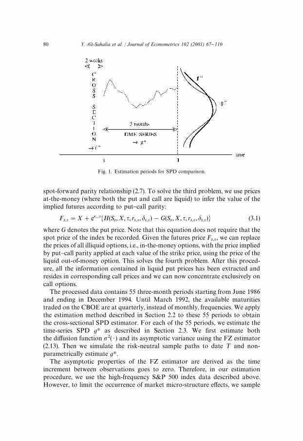
Fig. 1. Estimation periods for SPD comparison.

spot-forward parity relationship (2.7). To solve the third problem, we use pricesat-the-money (where both the put and call are liquid) to infer the value of theimplied futures according to put}call parity:

F��"X#e�� H(S

�,X, �, r

�� , �� )!G(S�,X, �, r

�� , ��) (3.1)

where G denotes the put price. Note that this equation does not require that thespot price of the index be recorded. Given the futures price F

�� , we can replacethe prices of all illiquid options, i.e., in-the-money options, with the price impliedby put}call parity applied at each value of the strike price, using the price of theliquid out-of-money option. This solves the fourth problem. After this proced-ure, all the information contained in liquid put prices has been extracted andresides in corresponding call prices and we can now concentrate exclusively oncall options.

The processed data contains 55 three-month periods starting from June 1986and ending in December 1994. Until March 1992, the available maturitiestraded on the CBOE are at quarterly, instead of monthly, frequencies. We applythe estimation method described in Section 2.2 to these 55 periods to obtainthe cross-sectional SPD estimator. For each of the 55 periods, we estimate thetime-series SPD gH as described in Section 2.3. We "rst estimate boththe di!usion function ��( ) ) and its asymptotic variance using the FZ estimator(2.13). Then we simulate the risk-neutral sample paths to date ¹ and non-parametrically estimate gH.

The asymptotic properties of the FZ estimator are derived as the timeincrement between observations goes to zero. Therefore, in our estimationprocedure, we use the high-frequency S&P 500 index data described above.However, to limit the occurrence of market micro-structure e!ects, we sample


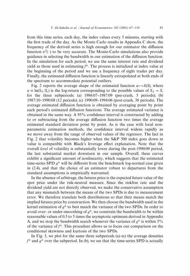
from this time series, each day, the index values every 5 minutes, starting withthe "rst trade of the day. As the Monte Carlo results in Appendix C show, thefrequency of the derived series is high enough for our estimator the di!usionfunction ��( ) ) to be very accurate. The Monte-Carlo simulations also provideguidance in selecting the bandwidth in our estimation of the di!usion function.In the simulation for each period, we use the same interest rate and dividendyield as those used in estimating fH. The process is initialized at index value atthe beginning of the period and we use a frequency of eight trades per day.Finally, the estimated di!usion function is linearly extrapolated at both ends ofthe spectrum to accommodate potential outliers.

Fig. 2 reports the average shape of the estimated function uC �( (S), whereu,ln(S

�/S

�) is the log-return corresponding to the possible values of S

�"S,

for the three subperiods: (a) 1986:07}1987:09 (pre-crash, 5 periods); (b)1987:10}1990:08 (12 periods); (c) 1990:09}1994:06 (post-crash, 38 periods). Theaverage estimated di!usion function is obtained by averaging point by pointeach period's estimated di!usion functions. The average estimated variance isobtained in the same way. A 95% con"dence interval is constructed by addingto or subtracting from the average di!usion function two times the averageestimated standard deviation point by point. As is the case with local non-parametric estimation methods, the con"dence interval widens rapidly aswe move away from the range of observed values of the regressor. The fact inFig. 2 that volatility becomes higher when the S&P 500 index goes down invalue is compatible with Black's leverage e!ect explanation. Note that theoverall level of volatility is substantially lower during the post-1990:09 period,the last substantial market downturn in our sample. Overall, these curvesexhibit a signi"cant amount of nonlinearity, which suggests that the estimatedtime-series SPD gH will be di!erent from the benchmark log-normal case givenin (2.4), and that the choice of an estimator robust to departures from thestandard assumptions is empirically warranted.

In the absence of arbitrage, the futures price is the expected future value of thespot price under the risk-neutral measure. Since the riskfree rate and thedividend yield are not directly observed, we make the conservative assumptionthat any mismatch between the means of the two SPDs is due to measurementerror. We therefore translate both distributions so that their means match theimplied futures price by construction.We then choose the bandwidth used in thekernel estimation of gH to best match the variance of the two SPDs. In order toavoid over- or under-smoothing of gH, we constrain the bandwidth to be withinreasonable values of 0.5 to 5 times the asymptotic optimum derived in AppendixA, and we stop the bandwidth search whenever the variance of gH is within 5%of the variance of fH. This procedure allows us to focus our comparison on theconditional skewness and kurtosis of the two SPDs.

In Fig. 3, we plot for the same three subperiods (a)}(c) the average densitiesfH and gH over the subperiod. In (b), we see that the time-series SPD is actually


Fig. 2. Average estimated � function.


Fig. 3. Average state price densities.


Table 1Bandwidth values for the SPD estimators�

Estimator Kernel Sample size q p m d h

X/F in fKH k��

n"2,520 2 5 2 2 h��

� in fKH k��

n"2,520 2 5 0 2 h��(��

in g( H k��

N"63 2 3 0 1 h��

g( H k��

M"10,000 2 3 0 1 h��

�Bandwidth selection for the SPD estimators, according to the selection rules given in Appendix A.All values in the table are averaged over the 52 three-month subperiods betweenApril 1986 and June1996.

more negatively skewed than the cross-sectional SPD, due to the October 1987market crash. The fact that from that point on fH will become more skewed (andmore leptokurtic) than gH is obviously consistent with the emergence of theimplied volatility smile after the market crash. More importantly, however, thedi!erences in skewness and kurtosis show that the options market has adjustedto pricing options according to a cross-sectional SPD that re#ects negativeskewness and excess kurtosis, but to a level that over-ampli"es their presence inthe time-series SPD. We now examine this last point in greater detail.

3.2. Comparing the cross-sectional and time-series SPDs

If investors had perfect foresight and knew the process governing the underly-ing asset price dynamics, then by no arbitrage, fH and gH should be equal. If thisassumption is too unrealistic } after all, the econometrician does not knowgH before the end of the estimation period, recall Fig. 1 } then we cannot expectall di!erences between the two SPDs in any given period to be traded away byarbitrageurs. However, we can still expect rational nonsatiated investors to takeadvantage of any systematic di!erences between the two SPDs that keep arisingover time. In much the same way, the CAPM is derived under the assumptionthat investors know the variance covariance matrix of the asset returns; hencein practice market e$ciency conclusions can only be drawn from repeateddeviations from the expected return relation. Therefore our comparisons ofthe two SPDs will focus only on the systematic di!erences between the twoimplied SPDs.

We document these di!erences in four di!erent ways. First, we focus on the"rst four conditional moments of the two SPDs. We start by regressing theconditional moments implied by fH on the corresponding moments implied bygH for the same period. If the moments estimated from option prices correctlyforecast the corresponding moments of the S&P 500 index through theirrespective SPDs, the intercept in the regression should be 0 and the slope shouldbe 1. Results in Table 2 indicate that the cross-sectional SPD fH systematically


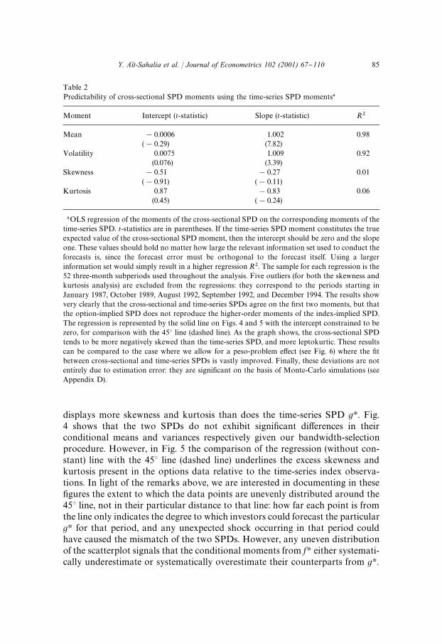
Table 2Predictability of cross-sectional SPD moments using the time-series SPD moments�

Moment Intercept (t-statistic) Slope (t-statistic) R�

Mean !0.0006 1.002 0.98(!0.29) (7.82)

Volatility 0.0075 1.009 0.92(0.076) (3.39)

Skewness !0.51 !0.27 0.01(!0.91) (!0.11)

Kurtosis 0.87 !0.83 0.06(0.45) (!0.24)

�OLS regression of the moments of the cross-sectional SPD on the corresponding moments of thetime-series SPD. t-statistics are in parentheses. If the time-series SPD moment constitutes the trueexpected value of the cross-sectional SPD moment, then the intercept should be zero and the slopeone. These values should hold no matter how large the relevant information set used to conduct theforecasts is, since the forecast error must be orthogonal to the forecast itself. Using a largerinformation set would simply result in a higher regression R�. The sample for each regression is the52 three-month subperiods used throughout the analysis. Five outliers (for both the skewness andkurtosis analysis) are excluded from the regressions: they correspond to the periods starting inJanuary 1987, October 1989, August 1992, September 1992, and December 1994. The results showvery clearly that the cross-sectional and time-series SPDs agree on the "rst two moments, but thatthe option-implied SPD does not reproduce the higher-order moments of the index-implied SPD.The regression is represented by the solid line on Figs. 4 and 5 with the intercept constrained to bezero, for comparison with the 453 line (dashed line). As the graph shows, the cross-sectional SPDtends to be more negatively skewed than the time-series SPD, and more leptokurtic. These resultscan be compared to the case where we allow for a peso-problem e!ect (see Fig. 6) where the "tbetween cross-sectional and time-series SPDs is vastly improved. Finally, these deviations are notentirely due to estimation error: they are signi"cant on the basis of Monte-Carlo simulations (seeAppendix D).

displays more skewness and kurtosis than does the time-series SPD gH. Fig.4 shows that the two SPDs do not exhibit signi"cant di!erences in theirconditional means and variances respectively given our bandwidth-selectionprocedure. However, in Fig. 5 the comparison of the regression (without con-stant) line with the 453 line (dashed line) underlines the excess skewness andkurtosis present in the options data relative to the time-series index observa-tions. In light of the remarks above, we are interested in documenting in these"gures the extent to which the data points are unevenly distributed around the453 line, not in their particular distance to that line: how far each point is fromthe line only indicates the degree to which investors could forecast the particulargH for that period, and any unexpected shock occurring in that period couldhave caused the mismatch of the two SPDs. However, any uneven distributionof the scatterplot signals that the conditional moments from fH either systemati-cally underestimate or systematically overestimate their counterparts from gH.


Fig. 4. Moment comparison.


Fig. 5. Moment comparison.


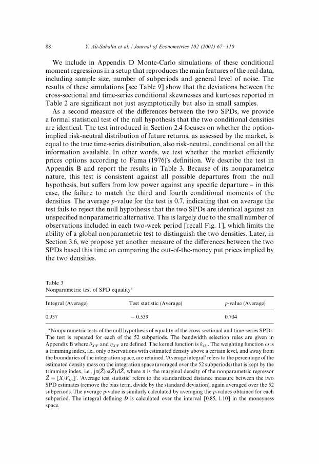
Table 3Nonparametric test of SPD equality�

Integral (Average) Test statistic (Average) p-value (Average)

0.937 !0.539 0.704

�Nonparametric tests of the null hypothesis of equality of the cross-sectional and time-series SPDs.The test is repeated for each of the 52 subperiods. The bandwidth selection rules are given inAppendix B where �

��and �

��are de"ned. The kernel function is k

��. The weighting function � is

a trimming index, i.e., only observations with estimated density above a certain level, and away fromthe boundaries of the integration space, are retained. &Average integral' refers to the percentage of theestimated density mass on the integration space (averaged over the 52 subperiods) that is kept by thetrimming index, i.e., ��(ZI )�(ZI ) dZI , where � is the marginal density of the nonparametric regressorZI "[X/F

��]. &Average test statistic' refers to the standardized distance measure between the twoSPD estimates (remove the bias term, divide by the standard deviation), again averaged over the 52subperiods. The average p-value is similarly calculated by averaging the p-values obtained for eachsubperiod. The integral de"ning D is calculated over the interval [0.85, 1.10] in the moneynessspace.

We include in Appendix D Monte-Carlo simulations of these conditionalmoment regressions in a setup that reproduces the main features of the real data,including sample size, number of subperiods and general level of noise. Theresults of these simulations [see Table 9] show that the deviations between thecross-sectional and time-series conditional skewnesses and kurtoses reported inTable 2 are signi"cant not just asymptotically but also in small samples.

As a second measure of the di!erences between the two SPDs, we providea formal statistical test of the null hypothesis that the two conditional densitiesare identical. The test introduced in Section 2.4 focuses on whether the option-implied risk-neutral distribution of future returns, as assessed by the market, isequal to the true time-series distribution, also risk-neutral, conditional on all theinformation available. In other words, we test whether the market e$cientlyprices options according to Fama (1976)'s de"nition. We describe the test inAppendix B and report the results in Table 3. Because of its nonparametricnature, this test is consistent against all possible departures from the nullhypothesis, but su!ers from low power against any speci"c departure } in thiscase, the failure to match the third and fourth conditional moments of thedensities. The average p-value for the test is 0.7, indicating that on average thetest fails to reject the null hypothesis that the two SPDs are identical against anunspeci"ed nonparametric alternative. This is largely due to the small number ofobservations included in each two-week period [recall Fig. 1], which limits theability of a global nonparametric test to distinguish the two densities. Later, inSection 3.6, we propose yet another measure of the di!erences between the twoSPDs based this time on comparing the out-of-the-money put prices implied bythe two densities.


3.3. The trading proxtability of SPD diwerences

Our third measure of the di!erences between the two SPDs consists inrecording the trading pro"ts that would have resulted from exploiting optimallytheir discrepancies. So far, we have identi"ed statistically signi"cant di!erencesbetween the cross-sectional SPD fH and the time-series SPD gH when comparingtheir conditional moments. We now propose to measure the di!erences betweenthe two SPDs using as a metric the pro"tability of trading from their di!erences.In Section 3.2, we were chie#y interested in whether the option market correctlyassesses at date t the time-series SPD that will prevail over the life of the option,i.e., in the period immediately following the option price observation: recallFig. 1. By contrast, trading decisions must obviously be made based on date t,not future, information and hence we must estimate both fH and gH with pastdata. We describe in Fig. 8 the estimation subperiods used at each point in timefor forming our trading portfolio. The cross-sectional SPD fH is estimated usingoption data within a window of two weeks following the latest expiration date,whereas the time-series SPD gH is estimated for a three-month period beforethat date. Option quotes on the business day immediately following the cross-sectional SPD estimation subperiod are used as the input of our tradingstrategy. We only take positions in out-of-the-money (OTM) and at-the-money(ATM) puts and calls, since these are more competitively priced due to theirliquidity. Thus our trading pro"ts are conservative in the sense that we haverestricted the investment opportunity set.

In Fig. 9, we indicate how to design such a trading strategy. Intuitively, we arebuying the range of strike prices which are underpriced in the sense of fH(gH

(prices, which are determined by fH, are cheaper than justi"ed by the time seriesgH) and selling options with payo!s in the ranges that are overpriced: fH'gH

(prices more expensive than justi"ed by the time series). Speci"cally, we takelong and short positions in options according to the rules described in Table 4.

In constructing our trading portfolio at time t, we value-weight each option inthe portfolio by their cash out#ow. The cash out#ow of a long position is thecost of the option itself; that of a short position is its margin deposit. We canthen measure the performance of our trading portfolio by its return. We de"nethe rate of return of the trading portfolio as

return"(total in#ow at expiration)/(total out#ow at initiation)!1. (3.2)

For simplicity, we assume that the margin deposit does not earn interest andshort sale proceeds cannot be used to "nance purchases. Based on our prior thatthe index option SPD is overly skewed and leptokurtic, we call &skewness trades'trades that are triggered by the rule (S1) only and &kurtosis trades' tradestriggered by rule (K1) only.

We report the results of these trading strategies in Table 5. It is clear from thetable that both trading strategies would have provided superior Sharpe ratios


Fig. 6. Moment comparison with jumps.


Fig. 7. Average relative price di!erence for out-of-the-money put.


Table 4Trading rules to exploit SPD di!erences�

Skewness (S1) skew( fH)'skew(gH) Sell OTM put,Buy OTM call

Trade (S2) skew( fH)(skew(gH) Buy OTM put,Sell OTM call

Kurtosis (K1) kurt( fH)'kurt(gH) Sell far OTM and ATM,Buy near OTM options

Trade (K2) kurt( fH)(kurt(gH) Buy far OTM and ATM,Sell near OTM options

�This table describes the trading rules designed to exploit the di!erences between the cross-sectional and time-series SPDs. A far OTM call (put) is de"ned as one whose strike price is 10%higher (lower) than the futures price. A near OTM call (put) is de"ned as one whose strike price is 5%higher (lower) but 10% lower (higher) than the futures price. The CBOE imposes speci"c marginrequirements on the S&P 500 index options. Uncovered writers must deposit 100% of the optionproceeds plus 15% of the aggregate contract value (current index level multiplied by $100) minus theamount by which the option is out-of-the money, if any. The minimummargin is 100% of the optionproceeds plus 10% of the aggregate contract value. Long puts or calls must be paid in full.

Table 5The pro"tability of trading SPD di!erences�

(S1) Skewness Trade

S&P 500Period Return Volatility Range Sharpe ratio Sharpe ratio

86:04}87:09 7.49 0.94 [7, 8] 1.8395 !0.089587:10}89:12 16.30 15.38 [!7, 47] 0.5680 0.347890:01}96:06 6.18 13.16 [!38, 21] 0.1346 0.1487Overall 8.79 13.79 [!38, 47] 0.2545 0.1106

(K1) Kurtosis Trade

S&P 500Period Return Volatility Range Sharpe ratio Sharpe ratio

86:04}87:09 !23.84 99.05 [!138, 41] !0.2985 !0.089587:10}89:12 17.58 21.38 [!18, 36] 0.4755 0.347890:01}96:06 21.50 24.94 [!44, 51] 0.6867 0.1487Overall 16.51 36.39 [!138, 51] 0.3145 0.1106

�This table reports the pro"t recorded from trading according to one of the two strategies (S1) or(K1) is measured as an annualized rate of return. The trading strategies are described in Fig. 7. Thereturns and their volatilities are all annualized. All numbers except Sharpe ratios are percentages.

(compared to buying and holding the S&P 500 index) over the 1986}1996period, as well as over the same three subperiods that we considered above.Given that the trading signal is based on the current option and the lagged indexobservations, the persistent trading pro"tability suggests that the relative shapes


of the SPDs evolve very slowly over time. The option SPD is overly skewed andleptokurtic in general, not period speci"c.

We will provide below a peso-problem interpretation for the superior pro"tsof the trading strategy. Indeed, by introducing a simple jump component to theindex dynamics to re#ect the nature of the peso problem, we are able to partiallyreconcile some of the di!erences in the time-series and cross-section SPDs. Boththe &skewness trades' and the &kurtosis trades' sell OTM puts, which couldconceivably incorporate a risk premium for the (downward) jump risk in theindex. By selling these options in a time period where ex post no jumps actuallyoccurred (but could have occurred ex ante), we are capturing this risk premiumin the form of superior returns.

3.4. Implications for the aggregate pricing kernel

Our option trading simulations based on the estimated SPD di!erencesachieves superior Sharpe ratios compared to buying and holding the S&P 500index over our sample period: see Table 5. We now explore a di!erent metric bywhich to assess the di!erences between the cross-sectional and time-seriesimplied state-price densities, or equivalently pricing kernels or stochastic dis-count factors. In this section, we look at the volatility of the stochastic discountfactor M that is consistent with our data. Hansen and Jagannathan (1991) showthat the "rst-order condition E(MR)"0 for the asset's excess return R impliesthe bound �(M)*E(M)E(R)/�(R) where the expectation and the standarddeviation are conditional on the information available at time t. The questionwe are now asking is how much tighter the bound is in the presence of options.

For a vector m of returns, the Hansen}Jagannathan bound without thepositivity restriction, M*0, becomes,

��(M)*(1!E(M)E(1#R))��(1!E(M)E(1#R)) (3.3)

where � is the variance}covariance matrix of the returns vector.We present the volatility bound of the stochastic discount factor in Fig. 10 in

the same format as Fig. 1 in Hansen and Jagannathan (1991, p. 228). The "gureshows the feasible region for the stochastic discount factor using the S&P 500index and T-bill (the solid line), and that using S&P 500 index, T-bill, and theoption portfolios (the dashed line). The option portfolios are from our skewnessand kurtosis trades reported in Table 5. For simplicity, the "gure does notimpose the nonnegativity restriction of the pricing kernel. Since we use oursample moments in our calculations, the short sample period and small numberof assets inevitably introduces measurement error. However, our goal is toillustrate the more stringent restriction on the volatility bound when the optionportfolio returns are included in our calculation.

In addition, we compare our volatility bounds obtained above to the volatil-ity of the stochastic discount factor under the consumption-CAPM. Here, we


Fig. 8. Estimation periods for trading SPD di!erences.

take the representative agent's preferences to be given by a time-separable powerutility function, ;(C)"(C��!1)/(1!�), where � is the coe$cient of relativerisk aversion, andC represents aggregate consumption. In this case, the stochas-tic discount factor is given at date t#1 by M

��"�(C

��/C

�)�, where � is the

subjective or time discount factor and C�is the level of aggregate consumption

at date t. We assume that consumption growth is an i.i.d. lognormal process. Wecalculate the volatility values of M corresponding to various values of the riskaversion parameter �. The volatility of M generated by the consumption data isalso plotted in Fig. 10. The "rst point above the horizontal axis has relative riskaversion of one; successive points have risk aversion of two, three, and so on; allvalues are obtained with �"1.0. Not surprisingly, the bound for M is morerestrictive in the presence of the option portfolios, although the restriction onthe risk aversion parameters is essentially comparable to the benchmark casewithout options: the power utility pricing kernels do not enter the feasible regionuntil the coe$cient of relative risk aversion reaches the value 27, vs. 26 withoutoptions.

3.5. Reconciling the implied SPDs: A peso-problem interpretation

A natural interpretation for the di!erences in skewness and kurtosis betweenfH and gH lies in the possible existence of a peso problem for the S&P 500 index:


the option market could price the S&P 500 options as if the S&P 500 index weresusceptible to large (downward) jumps of the type experienced in October 1987,even though jumps of that magnitude are absent from the time series data in thesubsequent period. A number of studies have documented the presence of jumpsin "nancial time series, and modeled their e!ect on option prices [see Bates(1991, 1996) and Bakshi et al. (1997)]. These studies have estimated the struc-tural parameters of the postulated SPD from the option data. They compare theoption-implied parameters to parameters estimated from the actual series of theunderlying asset value } not its risk-neutralized series } which is possiblethrough assumptions on preferences (typically log-utility or power utility). Ourfocus here is on the no-arbitrage restriction fH"gH, with the explicit objective ofavoiding assumptions on preferences.

In a context where realized jumps are infrequent, our estimates of thetime-series SPD would not be able to show any evidence of jumps; however, theestimated cross-sectional SPD would re#ect the existence of a jump risk as longas that risk is priced [Merton (1976) derives a closed-form option-pricingformula if this risk is unpriced]. To examine how the presence of jumps woulda!ect our empirical comparison of the two SPDs, we allow the risk-neutraldynamics of the index to contain a jump term in addition to its di!usioncomponent:

dSH�"(r

��!��!qH�H)SH

�dt#�(SH

�) d=H

�#JH

�SH�dNH

�(3.4)

where we specify that NH�

is a Poisson process with constant intensityqH (Pr(dNH

�"1)"qHdt), independent of =H

�, and for simplicity we make the

percentage jump size JH�nonrandom. The corresponding actual dynamics are

dS�"�(S

�) dt#�(S

�) d=

�#J

�S�dN

�(3.5)

where N�is a Poisson process with intensity q and the same jump times as NH

�,

and the percentage jump size is J�"JH

�"�H. The market price of jump risk is

qH/q.When we simulate dynamics (3.4), with the estimated �(

��( ) ), we will draw

observations from a process that incorporates the jump term. Over the multiplesample paths simulated, we will certainly observe some jumps, even thoughnone were present in the single sample path of the actual data } this isthe essence of the peso problem. Therefore, we use the same estimator of �( ) )as is the case where no jumps have been observed during the period of interest(three months in our empirical implementation). However, our estimatedtime-series SPD will re#ect the presence of the jumps because we are simulatinga large number of sample paths from a process where jumps are present,even though none were present in a single realization } the observed samplepath.


Table 6Skewness and kurtosis SPD "t in the presence of jumps�

No jump Jump frequency

10 yr 5 yr 3 yr 2 yr 1 yr

Skewness "t 0.5933 0.5344 0.5019 0.4806 0.5085 0.6964Kurtosis "t 1.6053 1.5187 1.4930 1.4947 1.5642 1.8014

�Root-mean-squared di!erences between the cross-sectional and time-series SPD moments, wherethe time series dynamics incorporate a jump term as in (3.4). The jump frequency parameter for thejump speci"cation is �H. The jump frequency is quoted in the table in terms of one jump per length oftime.

Note that the parameter qH/q, which enters the risk-neutral dynamics of theS&P 500, is determined by investors' preferences. In other words, we can nolonger fully identify the risk-neutral dynamics from the time series of actual S&P500 values. Instead, we will utilize the excess parameter qH to make the time-series SPD gH as close as possible to the cross-sectional SPD fH which wepreviously estimated. We still make no speci"c assumptions on preferences, aswe do not attempt to specify separately the actual jump intensity in (3.5). Speci"cpreferences would tell us how to go from (3.4) to (3.5), but that step is notrequired here since in a peso-problem context the observed Poisson processdoes not actually jump (i.e., the realized values in the sample are all dN

�"0).

Speci"cally, when jumps are possible, the equality fH"gH is no longer anover-identifying restriction since gH is no longer identi"able separately from theactual observations on �S

�. Instead, this equality allows us to restore the exact

identixcation of the system when previously it was an over-identifying restric-tion. As a result, there are no testable implications to be drawn, but we still fullyidentify the system without assumptions on preferences. Of course, if we werewilling to set bounds on the risk premium associated with the jump risk } orequivalently investors' risk aversion } then we could draw further conclusionsregarding the plausibility of the actual jump arrival intensity q correspondingto the estimated qH. Alternatively, we could use the additional restrictions givenby the equality between the two SPDs for di!erent option maturities. Thiswould then restore the overidenti"cation of the system and generate testableimplications.

Empirically, using post-1962 daily returns, we estimate the standard deviationof the S&P 500 index ex-dividend returns to be 0.855%. We classify negativereturns beyond "ve standard deviations to be downward jump events. There areseven such events out of the 8685 daily observations (roughly corresponds toonce every 5 year) with an average jump size of !8%. As a realistic speci"ca-tion, we therefore perform our simulations with a "xed downward jump size of!10%, and moment-matching scheme for four jump frequency speci"cations,


corresponding to one jump every ten years, "ve years, two years, and oneyear, respectively. The root mean squared (RMS) di!erences in Table 6between the cross-sectional and time-series (with jump) SPD moments exhibit aU-shaped pattern: the once-every-ten-years speci"cation does not produceenough skewness, whereas the once-every-two-years one results in a skewnessfor the time-series SPD that overshoots that of the cross-sectional SPD. We"nd that the minimum RMS is achieved for a frequency close to once everythree years. We therefore simulated (3.4) with this "fth jump frequency speci"ca-tion, which indeed produces a time-series SPD that best matches the cross-section SPD.

Fig. 6 is analogous to Fig. 5, but the time-series SPDs include the possibilityof jumps at the once-every-three-years frequency. Note that the scatter plot isnow more evenly distributed around the 453 axis, i.e., the conditional momentsof the cross-sectional SPD are matched more accurately when jumps areincluded than they were in Fig. 5. It is apparent that the incorporation of a jumpterm produces an improvement towards reconciling the cross-sectional andtime-series SPDs, but is not su$cient to explain the magnitude of the dispersionof the excess skewness and excess kurtosis of fH relative to gH. In particular, theinclusion of jumps reconciles the cross-sectional and time-series skewnessesbetter than it does for the corresponding kurtoses, which is to be expected sincewe have constrained the jumps to be exclusively of negative sign.

3.6. A comparison of out-of-the-money put prices

Our fourth and last measure of the di!erences between the two SPDs consistsin comparing the out-of-the-money put prices implied by the two distributions.Rather than comparing conditional moments, we are now comparing integralsof the option's payo! against the respective densities. For out of the moneyoptions, we are essentially computing (weighted) tail probabilities. Indeed,excess skewness and kurtosis implies that, other things being equal, out-of-the-money put options are more expensive. We report in Fig. 7 the relative averagedi!erence between the prices implied by both fH and gH. We obtain put pricesby integrating the left tail of the respective SPD against the respective putpayo!, and discounting at the riskfree rate. For a given moneyness level (de"nedas the ratio of the option's strike price to the S&P 500 futures price), we averagethe corresponding prices over the corresponding periods used in forming theSPD estimates. We "nally compute the relative di!erence between the pricesimplied by the fH and gH SPDs. As a result, excess skewness or kurtosisembedded in option prices should translate in a relative price di!erence whichgets larger as their moneyness is lower. Fig. 7 shows that this is indeed the caseespecially after the 1987 crash. Far out of the money puts valued using fH can beas much as 70% more expensive than their counterparts valued using gH.Further, Fig. 7 con"rms Fig. 6: it shows that the out-of-the-money put prices


Fig. 9. (a) Skewness trade. (b) Kurtosis trade.

implied by the time-series SPD when jumps are included are closer to thoseimplied by the cross-sectional SPD than the corresponding curve withoutjumps.


Fig. 10. Hansen}Jagannathan bound.

4. Conclusions

We have provided a method to infer from the observed time series of under-lying asset values the SPD that is directly comparable to the option-impliedSPD, and requires no assumptions on the representative preferences. We alsoshowed how separate exact identi"cation of the two SPDs from the observabledata can be achieved, leaving the theoretical restriction of equality between thetwo SPDs as an overidentifying restriction. In that context, the equality betweenthe cross-sectional and time-series SPDs becomes an over-identifying restric-tion, which is therefore testable. In addition to making no assumptions whatso-ever on preferences, we also avoided parametric assumptions on the nature ofthe di!usion driving the observable asset's price.

The extension of this method to the case of multiple traded state variablesposes no conceptual di$culties; in practice, our reliance on nonparametricestimators would result, in higher dimensions, in a loss of accuracy, and hencepower to detect deviations from one SPD to the other. This &curse of dimen-sionality' is a consequence of the local character of nonparametric estimators:accurate estimates can only be obtained in regions of the state space that are


visited often enough by the variables. For a given sample size, each region isrevisited much less often as the dimension gets higher. With this standard caveatin mind,Monte-Carlo evidence shows that our method performs very well in thecontext that was relevant for our empirical application.

In the case of the S&P 500 index, our comparison of the two SPDs revealsthat the market prices options with an overly skewed and leptokurtic SPD. Thuswe reject the joint hypothesis that the S&P 500 options are e$ciently priced andthat the S&P 500 index follows a one-factor di!usion. Trading schemes designedto exploit the SPD di!erences are able to produce superior pro"ts. The highSharpe ratios achieved by these trading schemes demand excessive variation ininvestors' marginal utilities, which further questions market e$ciency. Onepossible explanation for this evidence is the presence of an S&P 500 pesoproblem, whereby options incorporate a premium for the jump risk in theunderlying index that is absent from its recorded time series. We "nd someevidence in favor of that interpretation.

Moving away from the restrictive nature of the univariate di!usion speci"ca-tion, we were able to partly reconcile the di!erences between the index andoption implied SPDs by adding a jump component to the index dynamics. Theempirical results of this paper can therefore be interpreted alternatively asevidence of the limitations of a one-factor di!usion structure for the underlyingasset returns rather than an indictment on the rationality of the options markets.A further natural departure from this speci"cation would consist in incorporat-ing stochastic volatility to our speci"cation. Our method can be extended toincorporate the case where the volatility of the underlying asset is stochastic asa separate process, rather than stochastic only through its dependence on theasset price. The law of motion of the volatility process under the real probabilitymeasure can be estimated using standard "ltering techniques. However, giventhat volatility is a nontraded asset, its risk-neutral behavior cannot be solelyidenti"ed by estimating the di!usion function as in Section 2.3.1. We can stillestimate a three-dimensional option price function as in Section 2.2 (withvolatility as the additional, third, regressor). Then by applying Ito( 's lemma wecan derive the drift and di!usion function of any derivative price. In the absenceof arbitrage, the respective market prices of S&P 500 risk and volatility riskshould be identical for all derivative assets that are subject to these two sourcesof risk. This implies (as in the APT) that the instantaneous expected excessreturn of these derivative assets should be an average of the market prices of riskweighted by the size of their respective exposures, i.e., their di!usion coe$cients.Therefore, given the instantaneous expected excess returns and the di!usionfunction for options of two di!erent maturities, we can solve for the impliedmarket prices of risk. We can then obtain an overidentifying restriction bychecking if the implied market prices of risk are consistent with the derivedexpected instantaneous excess return and di!usion function for a di!erent set ofderivative prices, for instance options with a third maturity. Hence, we could


still, at least theoretically, test the validity of the model without resorting to anyassumptions on preferences.

Acknowledgements

We are grateful to David Bates, George Constantinides, Robert Engle andRobert MacDonald for useful discussions. Seminar participants also providedhelpful comments. This research was conducted in part during the "rst author'stenure as an Alfred P. Sloan Research Fellow. Financial support from the NSF(Grant SBR-9996023) and the University of Chicago's Center for Research inSecurity Prices is gratefully acknowledged.

Appendix A. Assumptions and asymptotic distributions

For each three-month subperiod, option prices form a panel data, consistingof N observation periods and J options per period. The sample size relevant forthe computation of the cross-sectional SPD fH is n"NJ, and N for thecomputation of the time-series SPD gH. We make the following assumptions onthe data used to construct the nonparametric regression (2.9), i.e., (�,ZI ) whereZI ,[X/F

�� , �]. The nonparametric regression function is �( (ZI ), and we wish toestimate its second partial derivative with respect to the "rst component X/F

��of the vector ZI .

Assumption A.1.

1. The process �>�,(�

�,ZI

�): i"1,2, n is strictly stationary with

E[��](R, E[��ZI

��](R

and is �-mixing with mixing coe$cients ��that decay as jPR at a rate at

least as fast as j�, b'19/2. The joint density of (>�,>

��) exists for all j and

is continuous.2. The density �(�,ZI ) is p-times continuously di!erentiable with respect to ZI ,

with p'm, and � and its derivatives are bounded and in ¸�(R��I ). The

marginal density of the nonparametric regressors, �(ZI ), is bounded awayfrom zero on every compact set in R�I .

3. �(ZI )�(ZI ) and its derivatives are bounded. The conditional variance

s�(ZI ),E[(�!�(ZI ))� � ZI ] (A.1)

is bounded and in ¸�(R�I ). The conditional fourth moment E[(�!�(ZI ))� � ZI ]

is bounded.


Dexnition A.1. A kernel function k is of order q if

��

�

z�k(z) dz"�1 if l"0

0 if 0(l(q

(!1)�q!��

if l"q

where l is an integer and ��

�z��k(z)�dz(R for all 0)l)q.

Assumption A.2. The kernel functions k��

and k� are bounded, three-timescontinuously di!erentiable, and have derivatives which are bounded and in¸�(R). k

��is of order q

��and k� is of order q� . The bandwidths are given by

h��

"c��

s(X/F)n��I ��, h�"c�s(�)n��I �� (A.2)

where s(X/F) and s(�) are the unconditional standard deviations of the non-parametric regressors, c

��,�

��/ln (n), with �

��constant, and c�,��/ln (n),

with �� constant.

In practice, we use the kernel functions

k��(z),e�

��/�2�, k��(z),(3!z�)e�

��/�8� (A.3)

which are of order q"2 and q"4 respectively. We then obtain, as in AmK t-Sahalia and Lo (1998), with ZI "[X/F

�� , �]:

Proposition A.1. Under Assumptions A.1 and A.2

n��h��

h�� [ fK H(S�)!fH(S

�)] �P N(0, ��

�H ) (A.4)

where �H��/�� is the option's gamma evaluated at �( (ZI ) and

��

H,�e�� H

��

(�( (ZI ), Z)��s�(ZI )(��

�(k��

��)�(�) d�)(��

�k�� (�) d�)

�(ZI )F��

. (A.5)

To estimate the time-series SPD gH, we make the following assumptions:

Assumption A.3. The drift function �( ) ) in (2.2) is a bounded function, twicecontinuously di!erentiable with bounded derivatives. The instantaneous volatil-ity function �( ) ) in (2.2) and (2.3) has three continuous and bounded derivatives,and there exist two constants c and C such that for all S.


Assumption A.4. The kernel function k��

is in ¸�(R) and is of order q

��"2. The

bandwidth h��

to form �(��( ) ), is given by

h��

"c��

N�� (A.6)

where c��

,��/ln(N), and �

��is a constant.

Assumption A.5. The kernel function k��

is in ¸�(R) and is of order q

��. The

bandwidth h��

is given by

h��

"c��

M�� (A.7)

where M is the number of Monte-Carlo simulations, c��

,��

/ln(M), and��

is a constant.

We discuss in Section 3 how we select the constants ��

and ��

. Letting thenumber of simulated sample paths of (2.3) go to in"nity, we obtain

Proposition A.2. Under Assumptions A.3 and A.4:

[g( H�(S

�)!gH

�(S

�)]"O

(N��). (A.8)

Appendix B. A nonparametric comparison test of fH"uH

To construct the estimators involved in the test statistic of Section 2.4, we usethe following bandwidth and kernel function, for the one-dimensionalsemiparametric model corresponding to ZI "[X/F

��]:

Assumption B.1. The bandwidth h��

to estimate fK H in (2.21) is given by

h��

"��

n��

where ��

is constant, and ��

satis"es

0(��

(2q��

#

9

2(B.1)

where q��

is the order of the kernel function k��

.

We then obtain

Proposition B.1. Under Assumptions A.1, A.3}A.5 and under H

nh��

D( fK H, g( H)!h��

B�

�P N(0,��) (B.2)


Table 7Kernel constants in asymptotic distributions�

Di!erentiation order m 0 1 2

��

(k��)�(w) dw �

��

��

��

��

��

(k��)�(w) dw ��

��

��

��

��

��

(��

k��(w)k��

��(w#v) dw)�dv �

��

��

��

�Kernel constants that characterize the asymptotic variances of the nonparametric estimators, andthe distribution of the test statistic. The kernel functions k

��and k

��are de"ned in (A.3). k�� denotes

the mth derivative of k.

where

B�

"��

�

k��(w) dw��ZI��(ZI )�� (ZI ) dZI (B.3)

��

"2��

��

��

�

k�(w)k�(w#v) dw��dv��ZI

��(ZI )�� (ZI ) dZI

(B.4)where

�� (ZI ),�e�� H

��(�(ZI ),Z)��

��(ZI ). (B.5)

Note that the sampling variation of g( H does not enter the asymptotic distribu-tion of the test statistic under H

, due to the faster rate of convergence of

g( H compared to fK H (compare (A.4) to (A.8)).To estimate consistently the conditional variance of the regression, s�(ZI )

we calculate the di!erence between the kernel estimate of the regression ofthe squared dependent variable �� on ZI and the squared of the regression �(ZI )of the dependent variable � on ZI . The regression E[�� ZI ] is estimatedwith bandwidth h

��"�

��n��), �

��"�� and �

��constant. The test statistic

is formed by standardizing the asymptotically normal distance measure D:we estimate consistently B

�and ��

�by plugging-in the estimate of the condi-

tional variance ��(ZI ), then subtract the asymptotic mean and divide by theasymptotic standard deviation. The test statistic then has the asymptotic N(0, 1)distribution. Since the test is one-sided (we only reject when D( fK H, g( H), hencethe test statistic, is large and positive), the 10% critical value is 1.28, while the5% value is 1.64. We "x the variables in Z that are excluded from ZI at theirsample means. Kernel constants appearing in Propositions A.1 and A.2 aregiven in Table 7.


Appendix C. Performance of the di4usion estimators in Monte-Carlo simulations

In our simulations, we set the drift of the log-return process to be constant at9% per year, which corresponds to the long-run historical ex-dividend average ofthe S&P 500 index. We calculate the volatility estimator with a given bandwidthh��

to each path and obtain the estimated volatility as a function of the price level.To investigate the sensitivity of the estimators to the choice of bandwidths, weevaluate the estimators over a range of possible bandwidth values. Two perfor-mance measures of the estimators are used for each choice of bandwidth.

We adopt as an evaluation criterion the mean integrated squared error(MISE) of the estimator. For each path, point-by-point squared estimationerrors (SE) are calculated. Then the SEs are weighted by their density (of S overall paths) and are summed up, producing the integrated squared error (ISE). Theaverage ISE over the 1000 paths becomes the MISE. However, the MISE doesnot explicitly tell how well the estimator captures the shape of the di!usionfunction. In fact it tends to favor the smoothness of the estimate over howaccurately the shape is captured. In practice, when estimating the di!usionfunction, we are not only interested in its level, but also its shape whichdetermines the skewness and the kurtosis of the time-series SPD gH.

Thus we propose a second performance measure that emphasizes how well theshape is captured (since the di!usion function is parametrically speci"ed, withparameters that determines the shape). The second measure describes how wellthe estimated di!usion function can reproduce these parameters. To obtain theestimated value �K "(a, b, c) of �"( ,�, �) for each path, we run an OLS regres-sion. The average of (a, b, c) over the 1000 paths are calculated.We then proceed totest the separate hypotheses "

, �"�

, �"�

(the subscript 0 denotes true

values) using the t-test, and the joint hypothesis �"� , using the ��-test. We then

select a bandwidth that balances MISE-minimization and shape preservation.In general, the FZ estimators capture the level and slope very well over almost

all shapes of volatility considered. The only exception is that the estimator tendsto under-estimate the slope as the volatility level gets lower. When the level andthe spread is large, FZ captures the curvature well, but not when the spread issmall and the level is low. However, one can argue that the ability to capture thecurvature is more crucial in the former case. To be closer to the theoreticalassumptions of FZ, we also generated paths using a small drift (3%) and foundthat it resulted in a slight improvement in the curvature estimation. Finally,when we increased the number of draws per day the performance of theestimator increased substantially, providing support for the asymptotic conver-gence results that we rely on. Table 8 summarizes quantitatively the estimator'sability to capture the shape of the �( ) ) for a variety of possible con"gurations. InFig. 11, we select four typical shapes of the true function �( ) ) and plot theaverage �(

��( ) ) estimated over all the simulated sample paths, as well as its 95%

Monte-Carlo con"dence interval.


Table 8Monte-Carlo simulations of the di!usion estimator�

Shape of ��( ) ) Estimation�( ��( ) )

Error�( ��

Relativeerror

Spread Slope Curvature Figure

Flat Flat Flat 11a 0.000233 0.000045 5.2Large Up Concave 0.000512 0.0229 0.02Large Up Flat 0.00106 0.00962 0.11Large Down Flat 11b 0.000871 0.0253 0.03Large Down Convex 0.00911 0.0323 0.28Small Up Flat 0.000699 0.0112 0.06Small Up Concave 11c 0.000808 0.0216 0.04Small Down Flat 0.000617 0.0129 0.05Small Down Convex 11d 0.000955 0.0294 0.03

�This table reports the results of Monte-Carlo simulations of the di!usion estimator for a varietyof shapes of the true di!usion function ��( ) ), which is parameterized as �(S)" #

�(S!S )#�(S!S

)�. The parameter is set at 0.20. A &large' spread represents the cases where

�"$0.002 and �"$0.00004, whereas a &small' spread corresponds to the cases where�"$0.001 and �"$0.00002. The sign of � and � determines the quali"ers up, down, concaveand convex in the usual sense. &Flat' corresponds to a parameter value of 0. The estimation errorreported in the table is the integrated mean squared error of the estimator (squared bias plusvariance), averaged over all the simulations. For each shape of the di!usion function, we have useda bandwidth that balances MISE-minimization and shape preservation. In the case where the truefunction is constant (and we know it), the maximum-likelihood estimator is naturally the moste$cient choice (see the "rst row of the table). However, in general the estimation error of �( �

��is less

than 5% of that of �( ��

.

Appendix D. Monte-Carlo simulations of the conditional moment regressions

In Table 9, we report the results of Monte-Carlo simulations of the condi-tional moments regressions used to compare the time-series and cross-sectionalconditional SPDmoments in Section 3.2, speci"cally Table 2. These simulationsare useful to assess the degree of small sample bias and variance inherent in theseconditional moments comparisons in conditions that approximate those of thereal data.

We replicate 500 economies with 11 year histories consisting of 55 subperiodseach. Each subperiod consists of 10,000 simulated sample paths for the underly-ing S&P 500 index assumed to follow Cox's CEV process

dSH�"(r!�)SH

�dt#�(SH

�)� d=H

�.

We set the initial value of the index at 450, the risk free rate r at 5% and thedividend payout rate � at 0%. For each period, we draw the volatility parameterfrom a normal distribution with mean of 35% (the real data average) anda standard deviation of 15%, with a cap and #oor of 70% and 5%, respectively.


Fig. 11. Monte-Carlo con"dence interval for the estimated �. (a) #at spread, #at slope, #atcurvature; (b) large spread, down slope, #at curvature; (c) small spread, up slope, concave curvature;(d) small spread, down slope, convex curvature.

We then calculate returns from the simulated paths and estimate the time-seriesSPD using the same estimator as with the real data. On the option side,we analytically price a cross-section of call options for each of the 55 periodsof the 500 sets using the closed-form CEV formula. The strikes range from 25%in the money to 35% out of the money. The time-to-maturity is three months, asin the real data. We use the same volatility parameter as that in the matchingindex simulation subperiod so that in the absence of noise and estimation errorthe two SPDs would by construction be identical. As with the real data, we thencompute the cross-sectional SPD for each of the 55 subperiods from theassociated cross-section of option prices. Since the cross-sectional moments aremore precisely estimated than their time-series counterparts, the regressions are


Table 9Monte-Carlo simulations of the conditional moments regressions�

Moment Intercept MC average(MC standard deviation)

Slope MC average(MC standard deviation)

R� MC average(MC standard deviation)

Mean !0.0004 1.019 0.73(0.001) (0.09) (0.06)

Volatility !0.002 0.988 0.99(0.006) (0.009) (0.001)

Skewness 0.012 1.08 0.75(0.03) (0.08) (0.06)

Kurtosis !0.14 1.22 0.42(0.11) (0.20) (0.10)

�This table reports the results of Monte-Carlo simulations of the conditional moment regressions.For each simulation, we compute the intercept and slope coe$cients and R� from a regression of theconditional moments using the simulated 55 subperiods. The table reports the mean and standarddeviations obtained from 500 overall simulations. The setup for the simulations is detailed inAppendix D and reproduces the main features of the real data, including sample size, number ofsubperiods and general level of noise. The results of these simulations show that the deviationsbetween the cross-sectional and time-series conditional skewnesses and kurtoses reported in Table 2are signi"cant in the sense of being outside their respective Monte-Carlo con"dence intervals.

corrected for the potential errors in variables problem (where y is regressed ona constant and x, with x measured with error) by inferring the coe$cients fromthe better-estimated reverse regression.

The closed-form expression of the CEV SPD is

fH�(S

�, S

�, �, r, �)"gH

�(S

�, S

�, �, r, �)

"

2S��

e��S��

S��

��

�I��

2�e��S��

S��

�(!1#e��)(1! )��

exp��

��

�� (!1#e��)��

where �"r!� (see Cox, 1996). This expression reduces to

fH�(S

�,S

�, �, r,�)"gH

�(S

�,S

�,�, r,�)"

2�� sinh�2e��S

�S��

(!1#e��)��exp�

(S��

#e��S��)�

(!1#e��)��!1#e��

for the absolute model ( "0).


References

AmK t-Sahalia, Y., 1996. Nonparametric pricing of interest rate derivative securities. Econometrica 64,527}560.

AmK t-Sahalia, Y., Duarte, J., 1999. Nonparametric option pricing under shape restrictions. Workingpaper, Princeton University.

AmK t-Sahalia, Y., Lo, A.W., 1998. Nonparametric estimation of state-price densities implicit in"nancial asset prices. Journal of Finance 53, 499}547.

AmK t-Sahalia, Y., Lo, A.W., 2000. Nonparametric risk management and implied risk aversion. Journalof Econometrics 94, 9}51.

Bakshi, G., Cao, C., Chen, Z., 1997. Empirical performance of alternative option pricing models.Journal of Finance 52, 2003}2049.

Banz, R., Miller, M., 1978. Prices for state-contingent claims: some estimates and applications.Journal of Business 51, 653}672.

Bates, D.S., 1991. The crash of '87: was it expected? The Evidence from Options Markets. Journal ofFinance 46, 1009}1044.

Bates, D.S., 1996. Jumps and stochastic volatility: exchange rate processes implicit in DeutscheMark options. Review of Financial Studies 9, 69}107.

Black, F., Scholes, M., 1973. The pricing of options and corporate liabilities. Journal of PoliticalEconomy 81, 637}659.

Breeden, D., Litzenberger, R., 1978. Prices of state-contingent claims implicit in option prices.Journal of Business 51, 621}651.

Canina, L., Figlewski, S., 1993. The informational content of implied volatility. Review of FinancialStudies 6, 659}681.

Chiras, D., Manaster, S., 1978. The informational content of option prices and a test of markete$ciency. Journal of Financial Economics 6, 213}234.

Cochrane, J.H., Hausen, L.P., 1992. Asset pricing explorations for macroeconomics, in NBER Macro-economics Annual, ed. by O. Blanchard and S. Fisher, MIT Press, Cambridge, MA, pp. 115}165.

Cox, J., 1996. The constant elasticity of variance option pricing model. The Journal of PortfolioManagement, Special Issue, 15}17.

Cox, J., Ross, S., 1976. The valuation of options for alternative stochastic processes. Journal ofFinancial Economics 3, 145}166.

Day, T., Lewis, C., 1988. The behavior of volatility implicit in the prices of stock index options.Journal of Financial Economics 22, 103}122.

Day, T., Lewis, C., 1990. Stock market volatility and the information content of stock index options.Journal of Econometrics 52, 267}287.

Derman, E., Kani, I., 1994. Riding on the smile. RISK 7, 32}39.Dumas, B., Flemming, J., Whaley, R.E., 1998. Implied volatility functions: empirical tests. Journal of

Finance 53, 2059}2106.Dupire, B., 1994. Pricing with a smile. RISK 7, 18}20.Engle, R.F., Mustafa, C., 1992. Implied ARCH models from option prices. Journal of Econometrics

52, 289}311.Fama, E.F., 1976. Foundations of Finance. Basil Books, New York, NY.Florens}Zmirou, D., 1993. On estimating the di!usion coe$cient from discrete observations.

Journal of Applied Probability 30, 790}804.Goldberger, D.H., 1991. A uni"ed method for pricing options on di!usion processes. Journal of

Financial Economics 29, 3}34.Hansen, L.P., Jagannathan, R., 1991. Implications of security market data for models of dynamic

economies. Journal of Political Economy 99, 225}262.Harrison, M., Kreps, D., 1979. Martingales and arbitrage in multiperiod securities markets. Journal

of Economic Theory 20, 381}408.


Harvey, C., Whaley, R., 1992. Market volatility prediction and the e$ciency of the S&P 100 indexoption market. Journal of Financial Economics 31, 43}73.

Jackwerth, J.C., 2000. Recovering risk aversion from option prices and realized returns. Workingpaper, London Business School.

Jackwerth, J.C., Rubinstein, M., 1996. Recovering probability distributions from contemporarysecurity prices. Journal of Finance 51, 1611}1631.

Jarrow, R., Rudd, A., 1982. Approximate option valuation for arbitrary stochastic processes. Journalof Financial Economics 10, 347}369.

Kloeden, P.E., Platen, E., 1992. Numerical Solution of Stochastic Di!erential Equations. Springer,Berlin, Germany.

Lo, A.W., Wang, J., 1995. Option pricing models when asset returns are predictable. Journal ofFinance 50, 87}129.

Longsta!, F., 1995. Option pricing and the martingale restriction. Review of Financial Studies 8,1091}1124.

Lamoureux, C.G., Lastrapes, W.D., 1993. Forecasting stock-return variance: toward an understand-ing of stochastic implied volatilities. Review of Financial Studies 6, 293}326.

Macbeth, J.D., Merville, L.J., 1979. An empirical examination of the Black}Scholes call optionpricing model. Journal of Finance 34, 1172}1186.

Mehra, R., Prescott, E.C., 1985. The equity premium: A puzzle. Journal of Monetary Economics 15,145}161.

Merton, R., 1973. Rational theory of option pricing. Bell Journal of Economics and ManagementScience 4, 141}183.

Merton, R., 1976. Option Pricing when Underlying Stock Returns are Discontinuous. Journal ofFinancial Economics 3, 125}144.

Ross, S., 1976. Options and e$ciency. Quarterly Journal of Economics 90, 75}89.Rubinstein, M., 1985. Nonparametric tests of alternative option pricing models using all reported

trades and quotes on the 30 most active CBOE option classes from August 23, 1976 throughAugust 31, 1978. Journal of Finance 40, 455}480.

Rubinstein, M., 1994. Implied binomial trees. Journal of Finance 49, 771}818.Schmalensee, R., Trippi, R.R., 1978. Common stock volatility expectations implied by option

premia. Journal of Finance 33, 129}147.Shimko, D., 1993. Bounds of probability. RISK 6, 33}37.Stutzer, M., 1996. A simple nonparametric approach to derivative security valuation. Journal of

Finance 51, 1633}1652.Wand, M.P., Jones, M.C., 1995. Kernel Smoothing. Chapman & Hall, London, UK.


Dooptionmarketscorrectlypricethe …yacine/comp.pdf ·...

Documents

Transcript of Dooptionmarketscorrectlypricethe …yacine/comp.pdf ·...