Donghwan Lee, Hyungjin Yoon, and Naira Hovakimyan

arX

iv:1

803.

0803

1v2

[m

ath.

OC

] 2

2 A

ug 2

018

Primal-Dual Algorithm for Distributed Reinforcement Learning: Distributed

GTD

Donghwan Lee, Hyungjin Yoon, and Naira Hovakimyan

Abstract— The goal of this paper is to study a distributedversion of the gradient temporal-difference (GTD) learningalgorithm for multi-agent Markov decision processes (MDPs).The temporal-difference (TD) learning is a reinforcement learn-ing (RL) algorithm which learns an infinite horizon discountedcost function (or value function) for a given fixed policy withoutthe model knowledge. In the distributed RL case each agentreceives local reward through a local processing. Informationexchange over sparse communication network allows the agentsto learn the global value function corresponding to a globalreward, which is a sum of local rewards. In this paper, theproblem is converted into a constrained convex optimizationproblem with a consensus constraint. Then, we propose aprimal-dual distributed GTD algorithm and prove that it almostsurely converges to a set of stationary points of the optimizationproblem.

I. INTRODUCTION

The goal of this paper is to study a distributed ver-

sion of the gradient temporal-difference (GTD) learning

algorithm, originally presented in [1], [2], for multi-agent

Markov decision processes (MDPs). There are N agents

i ∈ {1, . . . , N} =: V , which do not know the statistics of the

state transitions and rewards. Each agent i receives local re-

ward following a given fixed local policy πi. However, it will

be able to learn the global infinite horizon discounted cost

function (or value function) corresponding to the reward that

is a sum of local rewards through information exchange over

a sparse communication network. This paper only focuses

on the value evaluation problem with fixed local policies πi.However, the proposed approach can be extended to actor-

critic algorithms, which have multi-agent cooperative control

design applications.

A distributed Q-learning (QD-learning) was studied in [3].

The focus of [3] is to learn an optimal Q-factor [4] for a

global reward expressed as a sum of local rewards, while

each agent is only aware of its local reward. This work

therefore addresses the multi-agent optimal policy design

problem. If each agent has access to partial states and

actions, then the transition model of each agent becomes

non-stationary. This is because the state transition model of

each agent depends on the other agents’ policies. In [3], the

authors assumed that each agent observes the global state and

This work has been supported in part by the National Science Foundationthrough the National Robotics Initiative grant number 1528036, EAGERgrant number 1548409 and AFOSR grant number FA9550-15-1-0518.

D. Lee is with Coordinated Science Laboratory (CSL),University of Illinois, Urbana-Champaign, IL 61801, [email protected].

H. Yoon, and N. Hovakimyan are with the Department of Mechanical Sci-ence and Engineering, University of Illinois, Urbana-Champaign, IL 61801,USA [email protected], [email protected].

action; therefore, this non-stationary problem does not occur

in Q-learning settings. Distributed actor-critic algorithms

were explored in [5] with a similar setting. Each agent

acquires local observations and rewards, but it tries to learn

an optimal policy that maximizes the long-term average

of total reward which is a sum of local rewards. It was

assumed that each agent’s state-action does not change the

other agents’ transition models. In a more recent work [6],

consensus-based actor-critic algorithms were studied, where

the authors assumed that the transition model depends on

the joint action-states of all agents, and that each agent can

observe the entire combination of action-states.

In [7], a distributed policy evaluation was studied with the

GTD from [1], [2] combined with consensus steps. The study

focused on the scenario that there exists only one global

reward, each agnet behaves according to their own behavior

policy πi, and the agents cooperate to learn the value function

of the target policy π; thereby, it is a multi-agent off-policy

learning scheme. It was also assumed that each agent can

only explore a small subset of the MDP states. A consensus-

based GTD was also addressed in [8]. The authors considered

a problem similar to [7], and the weak convergence of the al-

gorithm was proved. In [9], a gossip-based distributed tempo-

ral difference (TD [4]) learning was investigated. Compared

to the previous work, the main difference in [9] is that all

agents know the global reward, but they have different linear

function approximation architectures with different features

and parameters of different dimensions. Agents cooperate to

find a value function with a linear function approximation

consisting of aggregated features of all agents to reduce

computational costs. Lastly, the papers [10], [11] addressed

distributed consensus-based stochastic gradient optimization

algorithms for general convex and non-convex objective

functions, respectively. Whenever the learning task can be

expressed as a minimization of an objective function, e.g.,

GTD [1], [2] or the residual method [12], algorithms in [10],

[11] can be applied. Besides, [13] studied a distributed

Newton method for policy gradient methods.

The main contribution of this paper is the development of

a new class of distributed GTD algorithm based on primal-

dual iterations as compared to the original one in [2]. The

most relevant previous studies which addressed the same

problem setting are [5], [6]. Even though [5], [6] studied

actor-critic algorithms, if the actor updates are ignored with

fixed policies, then they can deal with the same problem as

ours. The main difference compared to the previous result

is that the proposed algorithm incorporates the consensus

task into an equality constraint, while those in [5], [6]

http://arxiv.org/abs/1803.08031v2

use the averaging consensus steps explicitly. Therefore, our

algorithm views the problem as a constrained optimization,

and solves it using a primal-dual saddle point algorithm. The

proposed method is mainly motivated by [7], where the GTD

was interpreted as a primal-dual algorithm using Lagrangian

duality theory. The proposed algorithm was also motivated

by the continuous-time consensus optimization algorithm

from [14]–[16], where the consensus equality constraint was

introduced. The recent primal-dual reinforcement learning

algorithm from [17] also inspired the development in this

paper. We also note a primal-dual variant of the GTD in [18]

with proximal operator approaches.

One of the benefits of the proposed scheme is that the

consensus and learning tasks are unified into a single ODE.

Therefore, the convergence can be proved solely based on the

ODE methods [19]–[21], and the proof is relevantly simpler.

The second possible advantage is that the proposed algorithm

is a stochastic primal-dual method for solving saddle point

problems, and hence some analysis tools from optimization

perspectives, such as [17], can be applied (for instance, the

convergence speed and complexity of the algorithm), and

this agenda is briefly discussed at the end of the paper.

Full extension in this direction will appear in an extended

version of this paper. The third benefit of the approach

is that the method can be directly extended to the case

when the communication network is stochastic. In addition,

the proposed method can be generalized to an actor-critic

algorithm and off-policy learning. In this paper, we will focus

on a convergence analysis based on the ODE approach [19]–

[21]. Several open questions remain. For example, it is not

clear if there exists a theoretical guarantee that the proposed

algorithm improves previous consensus algorithms [5], [6],

[8]. Brief discussions are included in the example section.

II. PRELIMINARIES

A. Notation

The adopted notation is as follows: Rn: n-dimensional

Euclidean space; Rn×m: set of all n×m real matrices; AT :

transpose of matrix A; In: n× n identity matrix; I: identity

matrix with an appropriate dimension; ‖ · ‖: standard Eu-

clidean norm; for any positive-definiteD, ‖x‖D :=√xTDx;

for a set S, |S| denotes the cardinality of the set; E[·]:expectation operator; P[·]: probability of an event; for any

vector x, [x]i is its i-th element; for any matrix P , [P ]ijindicates its element in i-th row and j-th column; if z is a

discrete random variable which has n values and µ ∈ Rn is

a stochastic vector, then z ∼ µ stands for P[z = i] = [µ]i for

all i ∈ {1, . . . , n}; 1 denotes a vector with all entries equal

to one; dist(S, x): standard Euclidean distance of a vector xfrom a set S, i.e., dist(S, x) := infy∈S ‖x−y‖; for a convex

closed set S, ΓS(x) := argminy∈S ‖x− y‖.B. Graph theory

An undirected graph with the node set V and the edge set

E ⊆ V×V is denoted by G = (E ,V). We define the neighbor

set of node i as Ni := {j ∈ V : (i, j) ∈ E}. The adjacency

matrix of G is defined as a matrix W with [W ]ij = 1, if

and only if (i, j) ∈ E . If G is undirected, then W = WT .

A graph is connected, if there is a path between any pair of

vertices. The graph Laplacian is L = H −W , where H is

diagonal with [H ]ii = |Ni|. If the graph is undirected, then

L is symmetric positive semi-definite. It holds that L1 = 0.

We put the following assumption on the graph G.

Assumption 1: G is connected.

Under Assumption 1, 0 is a simple eigenvalue of L.

III. REINFORCEMENT LEARNING OVERVIEW

We briefly review basic RL algorithm from [22] with linear

function approximation for the single agent case. A Markov

decision process is characterized by a quadruple M :=(S,A, P, r, γ), where S is a finite state space (observations

in general),A is a finite action space, P (s, a, s′) := P[s′|s, a]is a tensor that represents the unknown state transition

probability from state s to s′ given action a, r : S ×A → R is the reward function, and γ ∈ (0, 1) is the

discount factor. The stochastic policy is a mapping π :S×A → [0, 1] representing the probability π(s, a) = P[a|s],rπ(s) : S → R is defined as rπ(s) := Ea∼π(s)[r(s, a)],P π denotes the transition matrix whose (s, s′) entry is

P[s′|s] = ∑

a∈A P[s′|s, a]π(s, a), and d : S → R denotes

the stationary distribution of the observation s ∈ S. The

infinite-horizon discounted value function with policy π and

reward r is

Jπ(s) := Eπ,P

[

∞∑

k=0

γk−1rπ(sk)

∣

∣

∣

∣

∣

s0 = s

]

,

where Eπ,P implies the expectation taken with respect to

the state-actor trajectories following the state transition Pand policy π. Given pre-selected basis (or feature) functions

φ1, . . . , φq : S → R, Φ ∈ R|S|×q is defined as a full column

rank matrix whose i-th row vector is[

φ1(i) · · · φq(i)]

.

The goal of RL with the linear function approximation is to

find the weight vector w such that Jw = Φw approximates

Jπ. This is typically done by minimizing the mean-square

Bellman error loss function [2]

minw∈Rq

MSBE(w) :=1

2‖rπ + γP πΦw − Φw‖2D , (1)

where D is a symmetric positive-definite matrix. For online

learning, we assume that D is a diagonal matrix with positive

diagonal elements d(s), s ∈ S. The residual method [12]

applies the gradient descent type approach wk+1 = wk −αk∇wMSBE(w)(w), where ∇wMSBE(w) = (γP πΦ −Φ)T (rπ + γP πΦw − Φw). In the model-free learning, the

gradient is replaced with a sample-based stochastic estimate.

A drawback of the residual method is that the next ob-

servation s′ should be sampled twice to obtain an unbi-

ased gradient estimate. In the TD learning [4], [22] with

a linear function approximation, the problem is resolved

by ignoring the first γP πΦ in the gradient ∇wMSBE(w):∇wMSBE(w) ∼= (−Φ)TD(rπ+γP πΦw−Φw). If the linear

function approximation is used, then this algorithm converges

to an optimal solution of (1). Compared to the residual

method, the double sampling issue does not occur. In the

above two methods, the fixed point problem rπ+γP πΦw =Φw may not have a solution in general because the left-hand

side need not lie in the range space of Φ. To address this

problem, the GTD in [2] solves instead the minimization of

the mean-square projected Bellman error loss function

minw∈Rq

MSPBE(w) :=1

2‖Π(rπ + γP πΦw − Φw)‖2D , (2)

where Π is the projection onto the range space of Φ, denoted

by R(Φ): Π(x) := argminx′∈R(Φ) ‖x−x′‖2D. The projection

can be performed by the matrix multiplication: we write

Π(x) := Πx, where Π := Φ(ΦTDΦ)−1ΦTD. Compared to

TD learning, the main advantage of GTD [1], [2] algorithms

are their off-policy learning abilities.

IV. DISTRIBUTED REINFORCEMENT LEARNING

OVERVIEW

Consider N reinforcement learning agents labelled

by i ∈ {1, . . . , N} =: V . A multi-agent Markov

decision process is characterized by the tuple

({Si}i∈V , {Ai}i∈V , P, {ri}i∈V , γ), where Si is a finite

state space (observations) of agent i, Ai is a finite action

space of agent i, ri : Si × Ai → R is the reward function,

γ ∈ (0, 1) is the discount factor, and P (s, a, s′) := P[s′|s, a]represents the unknown transition model of the joint state

and action defined as s := (s1, . . . , sN), a := (a1, . . . , aN ),

π(s, a) :=∏N

i=1 πi(si, ai), S :=N∏

i=1

Si, A :=N∏

i=1

Ai. The

stochastic policy of agent i is a mapping πi : Si×Ai → [0, 1]representing the probability πi(si, ai) = P[ai|si],rπi

i : Si → R is defined as rπi

i (si) := Eai∼πi(si)[ri(si, ai)],P π denotes the transition matrix, whose (s, s′) entry is

P[s′|s] =∑

a∈A1×···×ANP[s′|s, a]π(s, a), d : S → R

denotes the stationary distribution of the observation s ∈ S.

We assume that each agent can observe the entire joint

states s and local reward ri. We consider the following

assumption.

Assumption 2: With a fixed policy π, the Markov chain

P π is ergodic with the stationary distribution d with d(s) >0, s ∈ S.

Throughout the paper, D is defined as a diagonal matrix

with diagonal entries equal to those of d. The goal is to

learn an approximate value of the centralized reward rc =(rπ1

1 + · · ·+ rπN

N )/N .

Problem 1: The goal of each agent i is to learn an

approximate value function of the centralized reward rc =(rπ1

1 + · · · + rπN

N )/N without knowledge of its transition

model.

Remark 1: Possible scenarios of Problem 1 are summa-

rized as follows. Agents are located in a shared space, can

observe the joint states s from the environment, but get their

own local rewards. Another possibility is that each agent

has its own simulation environment and tries to learn the

value of their policy πi for the reward rπi

i . However, each

agent does not have access to other agents’ rewards due

to several reasons. For instance, there exists no centralized

coordinator; thereby each agent does not know other agents’

rewards. Another possibility is that each agent/coordinator

does not want to uncover their own goal or the global goal

for security/privacy reasons.

It can be proved that solving Problem 1 is equivalent to

solving

minw∈C

N∑

i=1

MSPBEi(w), (3)

where C ⊂ Rq is a compact convex set which includes the

unique unconstrained global minimum of (3).

Proposition 1: Solving (3) is equivalent to finding a so-

lution w∗ to the projected Bellman equation

Π

(

1

N

N∑

i=1

rπi

i + γP πΦw∗

)

= Φw∗. (4)

Proof: See Appendix .

Equivalently, the problem can be written by the consensus

optimization [23]

minwi∈C

N∑

i=1

MSPBEi(wi) (5)

subject to w1 = w2 = · · · = wN . (6)

To make the problem more feasible, we assume that its

learning parameter wi is exchanged via a communication

network represented by the undirected graph G = (E ,V).

V. PRIMAL-DUAL DISTRIBUTED GTD ALGORITHM

(PRIMAL-DUAL DGTD)

In this section, we study a distributed GTD algorithm. To

this end, we first define several vector and matrix notations

to save the space: w :=

w1

...

wN

, rπ :=

rπ1

1...

rπN

N

, P π :=

IN ⊗ P π, L := L ⊗ I|S|, D := IN ⊗ D, Φ := IN ⊗ Φ,

and B := ΦT D(I − γP π)Φ. If we consider the loss

function in (2), then the sum of loss functions in (5) can be

compactly expressed as∑N

i=1 MSPBEi(wi) =12 (Φ

T Drπ−Bw)T (ΦT DΦ)−1(ΦT Drπ−Bw). Noting that the consensus

constraint (6) can be expressed as

minw

1

2(ΦT Drπ − Bw)T (ΦT DΦ)−1(ΦT Drπ − Bw)

subject to Lw = 0

and motivated by [14]–[16], we convert it into the augmented

Lagrangian problem [24, sec. 4.2]

minw

1

2(ΦT Drπ − Bw)T (ΦT DΦ)−1(ΦT Drπ − Bw)+ wT LLw (7)

subject to Lw = 0.

If the system is known, the above problem is an equality

constrained quadratic programming problem, which can be

solved by means of convex optimization methods [25]. If

the model is unknown but observations can be sampled,

then the problem can be still solved by using stochastic

optimization techniques. To this end, some issues need to

be carefully taken into account. First, the objective function

evaluation involves the double sampling problem. Second,

the inverse in the objective function may lead to issues in

developing algorithms. In GTD [2], this problem is resolved

by a decomposition technique. In [7], it was proved that the

GTD can be related to the dual problem. Following the same

direction, we convert (7) into the equivalent optimization

problem

minε,h,w

1

2εT (ΦT DΦ)−1ε+

1

2hT h (8)

subject to

B I 0L 0 −IL 0 0

wεh

+

−ΦT Drπ

00

= 0,

where ε, h are newly introduced parameters. Its Lagrangian

dual can be derived by using standard approaches [25].

Proposition 2: The Lagrangian dual problem of (8) is

given by

minθ,v,µ

ψ(θ, v, µ) (9)

subject to BT θ − LT v − LT µ = 0,

where ψ(θ, v, µ) := 12 θ

T (ΦT DΦ)θ − θT ΦT Drπ + 12 v

T v.

Proof: The dual problem can be obtained by using the

standard manipulations in [25, Chap. 5].

As in [7], we again construct the Lagrangian func-

tion of (9), L(θ, v, µ, w) := ψ(θ, v, µ) + [BT θ −LT v − LT µ]T w, where w is the Lagrangian multiplier.

Since (9) satisfies the Slater’s condition [25, pp. 226], the

strong duality holds, i.e., maxw minθ,v,µ L(θ, v, µ, w) =minθ,v,µ maxw L(θ, v, µ, w), and the solutions of (9) are

identical to solutions (θ∗, v∗, µ∗, w) of the saddle point prob-

lem L(θ∗, v∗, µ∗, w) ≤ L(θ∗, v∗, µ∗, w∗) ≤ L(θ, v, µ, w∗).In addition, the saddle points (θ∗, v∗, µ∗, w) satisfying the

saddle point problem are identical to the KKT points

(θ∗, v∗, µ∗, w) satisfying

0 = ∇θL(θ∗, v∗, µ∗, w∗), 0 = ∇vL(θ

∗, v∗, µ∗, w∗),

0 = ∇µL(θ∗, v∗, µ∗, w∗), 0 = ∇wL(θ

∗, v∗, µ∗, w∗).(10)

It is known in [14], [15] that under a certain set of

assumptions the continuous gradient dynamics, dθdt =

−∇θL(θ, v, µ, w),dvdt = −∇vL(θ, v, µ, w),

dµdt =

−∇µL(θ, v, µ, w),dwdt = ∇wL(θ, v, µ, w), of the Lagrangian

function can solve the saddle point problem. The dynamic

systems can be compactly written by the ODE x = −Ax−b,where

A :=

ΦT DΦ 0 0 ΦT D(I − γP π)Φ0 I 0 −L0 0 0 −L

−ΦT (I − γP π)T DΦ L L 0

,

b :=

−ΦT Drπ

000

, x :=

θvµw

.

We first establish the fact that the set of stationary points of

the ODE x = −Ax − b corresponds to the set of optimal

solutions of the consensus optimization problem (6).

Proposition 3: Consider the ODE x = −Ax− b. The set

of stationary points of the ODE is given by R := {θ∗} ×{v∗}×F ×{w∗}, where v∗ = 0, w∗ = w∗

1 = · · · = w∗N , w∗

is the unique solution of the projected Bellman equation (4),

θ∗ = (ΦT DΦ)−1ΦT D(rπ− Φw∗+γP πΦw∗), and F is the

set of all solutions to the linear equation for µ

F := {µ : Lµ = ΦT (I − γP π)T DΦθ∗}. (11)


From Proposition 3 and Proposition 1, w∗ is the optimal

solution of (3). In addition, the stationary points in Proposi-

tion 3 are the KKT points given in (10). In addition, we can

prove that partial coordinates of the set of stationary points

in (3) are globally asymptotically stable.

Proposition 4: Consider the ODE x = −Ax − b. Then,

(θ, v, w)→ (θ∗, v∗, w∗) as t→∞.


Based on those observations, one can imagine a stochastic

approximation algorithm which can take benefits of the

properties of the ODE x = −Ax − b. In this respect, we

propose the distributed GTD (DGTD) in Algorithm 1, where

Cθ, Cv, Cµ, Cw are box constraints satisfying the following

assumption.

Assumption 3: The constraint sets satisfy θ∗ ∈ Cθ , v∗ ∈Cv , w∗ ∈ Cw, and Cµ ∩ F 6= ∅.The constraints are added to guarantee the stability and

convergence of the algorithm. According to [11, Prop. 4],

[20, Appendix E], the corresponding ODE is

x = ΓTC(x)(−Ax− b), (12)

where ΓTC(x) is defined as the projection of x onto the

tangent cone TC(x) [24, pp. 343] of C := Cθ×Cv×Cµ×Cw

at x. Due to the additional constraints, the set of stationary

points of (12) is a larger set, which includes those of x =−Ax − b as a subset. The following results can be directly

proved using the definitions of tangent and normal cones [24,

pp. 343].

Proposition 5: The set of stationary points of (12) is P :={x ∈ C : ΓTC(x)(−Ax − b) = 0} = {x ∈ C : −Ax − b ∈NC(x)}.We first establish the convergence of Algorithm 1 to the

stationary points of (12) under the standard diminishing step

size rule [23]

αk > 0, ∀k ≥ 0,

∞∑

k=0

αk =∞,∞∑

k=0

α2k <∞. (13)

Proposition 6 (Convergence of DGTD): Define

θk :=

θ1,k...

θN,k

, vk :=

v1,k...

vN,k

, µk :=

µ1,k

...µN,k

, wk :=

w1,k

...wN,k

,

and xk :=[

θTk vTk µTk wT

k

]Twith iterations in Algo-

rithm 1. With the step size rule (13), dist(xk,P) → 0 as

k → ∞, where P := {x ∈ C : −Ax − b ∈ NC(x)} with

probability one.


Algorithm 1 Distributed GTD algorithm (DGTD)

1: Initialize {θ(i)0 }i∈V and set k = 0.

2: repeat

3: k ← k + 14: for agent i ∈ {1, . . . , N} do

5: Sample (s, a, s′) with s ∼ di(s), a ∼πi(a|s), s′ ∼ pi(s

′|s, a) and update parameters accord-

ing to

θi,k+1/2 =θi,k − αk[φφT θi,k + φφTwi,k

− γφ(φ′)Twi,k − φrπi

i ]

vi,k+1/2 =vi,k − αk

vi,k −

|Ni|wi,k −∑

j∈Ni

wj,k

,

µi,k+1/2 =µi,k + αk

|Ni|wi,k −∑

j∈Ni

wj,k

,

wi,k+1/2 =wi,k − αk

|Ni|vi,k −∑

j∈Ni

vj,k

− αk

|Ni|µi,k −∑

j∈Ni

µj,k

+ αk(φφT θi,k − γφ′φT θi,k),

where Ni is the neighborhood of node i on the graph G,

φ := φ(s), φ′ := φ(s′), rπi

i := rπi

i (s).6: Project the iterates θi,k+1 = ΓCθ

[θi,k+1/2],vi,k+1 = ΓCv

[vi,k+1/2], µi,k+1 = ΓCµ[µi,k+1/2],

wi,k+1 = ΓCw[wi,k+1/2].

7: end for

8: until a certain stopping criterion is satisfied.

Although Proposition 6 states that the iterations of Propo-

sition 6 converge to a stationary point of the projected

ODE (12), it does not guarantee that they converge to the

set of stationary points of the ODE without the projection

in Proposition 3. In practice, however, we expect that they

may often converge to the set in Proposition 3, if the

constraint sets are sufficiently large. On the other hand, if we

follow the analysis of the stochastic primal-dual algorithm

in [17], we can prove that under certain conditions, the

iterations of Algorithm 1 converge to the the stationary points

in Proposition 3. The proof is similar to those in [17], and

we defer its full analysis to an extended version of this paper.

VI. EXAMPLES

Example 1: Consider a stock market whose price pro-

cess is approximated by a Markov chain with 100

states S := {$10, $20, . . . , $1000}. If an agent buys

a stock, then it loses s ∈ S, and if sells, then it

earns s ∈ S. Define the trading policy π(s; a, b) =

{

If a ≤ s ≤ b, then buy a stock

Otherwise, sell a stock. There are five trading

agents V = {1, 2, . . . , 5} with different private policies

π1(s) = π(s; $10, $30), π2(s) = π(s; $10, $40), π3(s) =π(s; $10, $50), π4(s) = π(s; $10, $60), and π5(s) =π(s; $10, $70). To determine an investment strategy, each

agent is interested in estimating an average of long term

discounted profits of all agents as well as its own. When the

current state is s ∈ S, the reward of each agent is rπi

i = −sif πi = buy, and rπi

i = s if πi = sell. For this example, we

used Gaussian radial basis functions as features of the linear

function approximation with 11 parameters, i.e., wi ∈ R11,

we considered the discount factor γ = 0.5, and we used a

randomly generated Markov chain for the stock price process

model. Using the single agent GTD [2], each agent computed

the approximate value functions Jw∗

i= Φw∗

i , i ∈ V . The

expected profits with the uniform initial state distribution

are Es∼U(S)[Jw∗

1(s)] = 164.3, Es∼U(S)[Jw∗

2(s)] = 55.6,

Es∼U(S)[Jw∗

3(s)] = −107.5, Es∼U(S)[Jw∗

4(s)] = −240.4,

and Es∼U(S)[Jw∗

5(s)] = −284.4639, where U(S) is the

uniform distribution over the state S. Using the single agent

GTD again, the value function Jw∗

c= Φw∗

c (global value

function) corresponding to the central reward rc = (r1 +r2 + r3 + r4 + r5)/5 was computed, and the expected profit

is Es∼U(S)[Jw∗

c(s)] = −82.5. Since each agent wants to keep

its profit secure, agent i can compute its own value function

Jw∗

ionly. However, there are associated agents, which are

able to exchange their parameters. The associate relations are

depicted in Figure 1. Under this assumption, Algorithm 1

Fig. 1. Graph describing the associate relations among five trading agents.

was applied with the step size rule αk = 10/(k+1000) and

without the projections, and each agent computed the global

value function estimations Jw∗

i= Φw∗

i , i ∈ V . The result

of 50000 iterations with a single simulation trajectory is

illustrated in Figure 2. Distinguished by different colors, the

consensus of 11 parameters of wi for five agents is shown.

The same color is used for each coordinate of all the agents.

The expected profits with uniform initial state distribution

are Es∼U(S)[Jw∗

1(s)] = −83.2, Es∼U(S)[Jw∗

2(s)] = −85.0,

Es∼U(S)[Jw∗

3(s)] = −81.2, Es∼U(S)[Jw∗

4(s)] = −83.5, and

Es∼U(S)[Jw∗

5(s)] = −79.5. This result demonstrates that

each agent successfully estimated the global value function

Jw∗

c= Φw∗

c . Even though we are not aware of previous

methods on the same topic, we combined the standard con-

sensus method with GTD and compared the result with Fig-

ure 2. We observed that the convergence of Figure 2 is

usually faster than the standard consensus approach.

0.5 1 1.5 2 2.5 3 3.5 4 4.5 5

x 104

−100

−50

0

50

100

Iterations

w1,w

2,...,w

5

Fig. 2. Example 1: Convergence of 11 parameters (distinguished bydifferent colors) of five agents (not distinguished by colors).

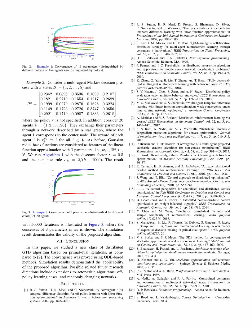
Example 2: Consider a multi-agent Markov decision pro-

cess with 5 states S := {1, 2, . . . , 5} and

P π =

0.2362 0.0895 0.3536 0.1099 0.21070.1821 0.2719 0.1553 0.1217 0.26890.1999 0.0279 0.2870 0.1628 0.32240.1149 0.1723 0.2726 0.3747 0.06560.2921 0.1719 0.0907 0.1836 0.2618

,

where the policy π is not specified. In addition, consider 20

agents V = {1, 2, . . . , 20}. They exchange their parameters

through a network described by a star graph, where the

agent 1 corresponds to the center node. The reward of each

agent i is rπi

i ≡ i for all i ∈ V . As before, Gaussian

radial basis functions are considered as features of the linear

function approximation with 3 parameters, i.e., wi ∈ R3, i ∈

V . We run Algorithm 1 with the discount factor γ = 0.5and the step size rule αk = 2/(k + 1000). The result

0.5 1 1.5 2 2.5 3 3.5 4 4.5 5

x 104

0

2

4

6

8

10

12

Iterations

w1,w

2,w3

Fig. 3. Example 2: Convergence of 3 parameters (distinguished by differentcolors) of 20 agents.

with 50000 iterations is illustrated in Figure 3, where the

consensus of 3 parameters in wi is shown. The simulation

result demonstrates the validity of the proposed algorithm.

VII. CONCLUSION

In this paper, we studied a new class of distributed

GTD algorithm based on primal-dual iterations, as com-

pared to [2]. The convergence was proved using ODE-based

methods. Simulation results demonstrated the applicability

of the proposed algorithm. Possible related future research

directions include extensions to actor-critic algorithms, off-

policy learning cases, and randomly changing networks.

REFERENCES

[1] R. S. Sutton, H. R. Maei, and C. Szepesvari, “A convergent o(n)temporal-difference algorithm for off-policy learning with linear func-tion approximation,” in Advances in neural information processing

systems, 2009, pp. 1609–1616.

[2] R. S. Sutton, H. R. Maei, D. Precup, S. Bhatnagar, D. Silver,C. Szepesvari, and E. Wiewiora, “Fast gradient-descent methods fortemporal-difference learning with linear function approximation,” inProceedings of the 26th Annual International Conference on Machine

Learning, 2009, pp. 993–1000.

[3] S. Kar, J. M. Moura, and H. V. Poor, “QD-learning: a collaborativedistributed strategy for multi-agent reinforcement learning throughconsensus + innovations,” IEEE Transactions on Signal Processing,vol. 61, no. 7, pp. 1848–1862, 2013.

[4] D. P. Bertsekas and J. N. Tsitsiklis, Neuro-dynamic programming.Athena Scientific Belmont, MA, 1996.

[5] P. Pennesi and I. C. Paschalidis, “A distributed actor-critic algorithmand applications to mobile sensor network coordination problems,”IEEE Transactions on Automatic Control, vol. 55, no. 2, pp. 492–497,2010.

[6] K. Zhang, Z. Yang, H. Liu, T. Zhang, and T. Basar, “Fully decentral-ized multi-agent reinforcement learning with networked agents,” arXiv

preprint arXiv:1802.08757, 2018.

[7] S. V. Macua, J. Chen, S. Zazo, and A. H. Sayed, “Distributed policyevaluation under multiple behavior strategies,” IEEE Transactions on

Automatic Control, vol. 60, no. 5, pp. 1260–1274, 2015.

[8] M. S. Stankovic and S. S. Stankovic, “Multi-agent temporal-differencelearning with linear function approximation: weak convergence undertime-varying network topologies,” in American Control Conference(ACC), 2016, pp. 167–172.

[9] A. Mathkar and V. S. Borkar, “Distributed reinforcement learning viagossip,” IEEE Transactions on Automatic Control, vol. 62, no. 3, pp.1465–1470, 2017.

[10] S. S. Ram, A. Nedic, and V. V. Veeravalli, “Distributed stochasticsubgradient projection algorithms for convex optimization,” Journal

of optimization theory and applications, vol. 147, no. 3, pp. 516–545,2010.

[11] P. Bianchi and J. Jakubowicz, “Convergence of a multi-agent projectedstochastic gradient algorithm for non-convex optimization,” IEEE

Transactions on Automatic Control, vol. 58, no. 2, pp. 391–405, 2013.

[12] L. Baird, “Residual algorithms: Reinforcement learning with functionapproximation,” in Machine Learning Proceedings 1995, 1995, pp.30–37.

[13] R. Tutunov, H. B. Ammar, and A. Jadbabaie, “An exact distributednewton method for reinforcement learning,” in 2016 IEEE 55th

Conference on Decision and Control (CDC), 2016, pp. 1003–1008.

[14] J. Wang and N. Elia, “Control approach to distributed optimization,”in 48th Annual Allerton Conference on Communication, Control, and

Computing (Allerton), 2010, pp. 557–561.

[15] ——, “A control perspective for centralized and distributed convexoptimization,” in 50th IEEE Conference on Decision and Control andEuropean Control Conference (CDC-ECC), 2011, pp. 3800–3805.

[16] B. Gharesifard and J. Cortes, “Distributed continuous-time convexoptimization on weight-balanced digraphs,” IEEE Transactions on


[17] Y. Chen and M. Wang, “Stochastic primal-dual methods andsample complexity of reinforcement learning,” arXiv preprint

arXiv:1612.02516, 2016.

[18] S. Mahadevan, B. Liu, P. Thomas, W. Dabney, S. Giguere, N. Jacek,I. Gemp, and J. Liu, “Proximal reinforcement learning: A new theoryof sequential decision making in primal-dual spaces,” arXiv preprint

arXiv:1405.6757, 2014.

[19] V. S. Borkar and S. P. Meyn, “The ODE method for convergence ofstochastic approximation and reinforcement learning,” SIAM Journalon Control and Optimization, vol. 38, no. 2, pp. 447–469, 2000.

[20] S. Bhatnagar, H. Prasad, and L. Prashanth, Stochastic recursive algo-

rithms for optimization: simultaneous perturbation methods. Springer,2012, vol. 434.

[21] H. Kushner and G. G. Yin, Stochastic approximation and recursive

algorithms and applications. Springer Science & Business Media,2003, vol. 35.

[22] R. S. Sutton and A. G. Barto, Reinforcement learning: An introduction.MIT Press, 1998.

[23] A. Nedic, A. Ozdaglar, and P. A. Parrilo, “Constrained consensusand optimization in multi-agent networks,” IEEE Transactions on


[24] D. P. Bertsekas, Nonlinear programming. Athena scientific Belmont,1999.

[25] S. Boyd and L. Vandenberghe, Convex Optimization. CambridgeUniversity Press, 2004.

APPENDIX

Since (3) is strongly convex, its unconstrained global

minimum is unique, and it satisfies

∇w

N∑

i=1

MSPBEi(w) = −(ΦTD(I − γP π)Φ)T

× (ΦTDΦ)−1ΦTDN∑

i=1

(rπi

i − (I − γP π)Φw) = 0.

Since ΦTD(I − γP π)Φ is nonsingular [4, pp. 300], this

implies

(ΦTDΦ)−1ΦTD

N∑

i=1

(rπi

i − (I − γP π)Φw) = 0.

Pre-multiplying the equation by Φ yields the desired result.

The proof is based on the analysis of the stochastic

recursion

xk+1 = ΓC(f(xk) + εk). (14)

Define the σ-field Fk :=σ(ε0, . . . , εk−1, x0, . . . , xk, α0, . . . , αk). According to [11,

Prop. 4], [20, Appendix E], the corresponding ODE can be

expressed as

x = ΓTC(x)[f(x)].

We consider assumptions listed below.

Assumption 4:

1) The function f : RN → RN is continuous.

2) The step sizes satisfy

αk > 0, ∀k ≥ 0,

∞∑

k=0

αk =∞, αk → 0 as k →∞.

3) The ODE x = ΓTC(x)[f(x)] has a compact subset Pof R

N as its set of asymptotically stable equilibrium

points.

Let t(k), k ≥ 0 be a sequence of positive real numbers

defined according to t(0) = 0 and t(k) =∑k−1

j=0 αj , k ≥ 1.

By the step size in Assumption 4, t(k) → ∞ as k → ∞.

Define m(t) := max{k|t(k) ≤ t}. Thus, m(t) → ∞ as

t→∞.

Assumption 5: There exists T such that for all δ > 0

limk→∞

P

supj≥k

max0≤t≤T

∥

∥

∥

∥

∥

∥

m(jT+t)−1∑

i=m(jT )

αiεi

∥

∥

∥

∥

∥

∥

≥ δ

= 0. (15)

Lemma 1 (Kushner and Clark Theorem [21, Appendix E]):

Under Assumption 4 and Assumption 5, for any initial

x(0) ∈ RN , x(k)→ P as k→∞ with probability one.

Proof of Proposition 6: We will check Assumption 4

and Assumption 5 and use Lemma 1 to complete the proof.

The ODE in (12) is a projection of an affine map f(x) =−Ax−b; therefore, it is obviously continuous. The step size

assumption is satisfied by the hypothesis. In addition, the set

of stationary points P = {x ∈ C : ΓTC(−Ax − b) = 0} is

compact. This is because P is expressed as P = {x ∈ C :−Ax− b ∈ NC(x)}, where NC(x) is a convex closed cone,

and its pre-image of an affine map is also closed. Therefore,

P is closed. P ⊆ C, because ΓTC(−Ax − b) = 0 only

when x ∈ C. Since C is compact and P is its closed subset,

P is also compact. P can be also proved to be globally

asymptotically stable following analysis given in [11]. For

completeness of the presentation, the brief proof is given in

Appendix . Next, we will prove Assumption 5. Proposition 6

can be expressed as (14) with εk = (−Axk−b)−(−Axk−b),where −Axk − b is a stochastic approximate of −Axk −b such that E[−Axk − b|Fk] = −Axk − b. Therefore,

E[εk|Fk] = 0. Define Mk :=∑k−1

i=0 αiεi. Then, since

E[Mk+1|Fk] =Mk, (Mk)∞k=0 is a Martingale sequence. We

will prove the sufficient condition for (15).

limk→∞

P

max0≤t≤T

∣

∣

∣

∣

∣

∣

m(kT+t)−1∑

i=m(kT )

αiεi

∣

∣

∣

∣

∣

∣

≥ δ

= 0.

Since max0≤t≤T

∥

∥

∥

∑m(kT+t)−1i=m(kT ) αiεi

∥

∥

∥ ≤maxm(kT )≤t≤m(kT+T )−1

∥

∥

∥

∑ti=m(kT ) αiεi

∥

∥

∥, we will

consider a more conservative sufficient condition:

limk→∞

P

(

max0≤t≤m(kT+T )−m(kT )−1

‖Ht‖ ≥ δ)

= 0, (16)

where (Ht)∞t=0 with Ht :=

∑m(kT )+ti=m(kT ) αiεi is a Martingale

sequence. Then, by using the Martingale inequality, we have

P

(

max0≤t≤m(kT+T )−m(kT )−1

|Ht| ≥ δ)

≤E

[

∣

∣

∣

∑m(kT+T )−1i=m(kT ) αiεi

∣

∣

∣

2]

δ2≤C2∑∞

i=m(kT ) α2i

δ2,

where we used ‖εi‖2 ≤ C2. By the step size rule in (13),∑∞

k=0 α2k < ∞ implies that the right-hand side converges

to zero as k → ∞. Therefore, we prove (16) and (15).

By Lemma 1, we prove that xk globally converges to the

stationary point H with probability one.

In this section, we will prove the following claim.

Proposition 7: Consider the ODE x = ΓTC(x)(−Ax −b) in (12). The set of stationary points H = {x ∈ C :ΓTC

(−Ax− b) = 0} is globally asymptotically stable.

The proof is given in [11], and we provide a brief sketch of

the proof.

Proof: If we define the function V (x) :=xT (Ax + b), then the ODE can be represented by x =ΓTC(x)(−∇xV (x)). Let V (x) be a candidate Lyapunov

function for P . Then, its time derivative is expressed as

V (x) = ∇xV (x)TΓTC(x)(−∇xV (x)). Since ∇xV (x) =ΓTC(x)(∇xV (x)) + ΓNC(x)(∇xV (x)), and the tangent cone

and normal cone are orthogonal, we arrive at V (x) =

−∥

∥ΓTC(x)(−∇xV (x))∥

∥

2. Therefore, P = {x ∈ C :

ΓTC(x)(−∇xV (x)) = 0} = {x ∈ C : −∇xV (x) ∈ NC(x)}is globally asymptotically stable. Since −∇xV (x) = −Ax−b, the proof is completed.

We first consider the stationary points of (12) without the

projection. They are obtained by solving the linear equation:

0 = (ΦT DΦ)θ − ΦT Drπ + ΦT D(I − γP π)Φw, (17)

0 = v − Lw, (18)

0 = Lw, (19)

0 = Lv + Lµ− ΦT (I − γP π)T DΦθ. (20)

Since G is connected by Assumption 1, the dimension of the

null space of L is one. Therefore, span(1) is the null space.

Therefore, (19) implies the consensusw∗ = w∗1 = · · · = w∗

N ,

and plugging (19) into (18) yields v∗ = 0. With v∗ = 0, (20)

is simplified to

Lµ∗ = ΦT (I − γP π)T DΦθ∗. (21)

In addition, from (17), the stationary point for θ satisfies

θ∗ = (ΦT DΦ)−1ΦT D(rπ − Φw∗ + γP πΦw∗). (22)

Plugging the above equation into (21) yields

Lµ = ΦT (I − γP π)T DΦθ

= ΦT (I − γP π)T DΦ(ΦT DΦ)−1

× ΦT D(rπ − Φw + γP πΦw). (23)

Multiplying (23) by (1⊗ I)T on the left results in

N∑

i=1

([Φ− γP πΦ]TDΦ(ΦTDΦ)−1

ΦTD[−rπi

i +Φw∗ − γP πΦw∗]) = 0,

which is equivalent to∑N

i=1∇wMSPBEi(w∗) = 0. Since

the loss functions are strict convex quadratic functions,

w∗ is the unique global minimum of∑N

i=1 MSPBEi(w).From (22), θ∗ is also uniquely determined. In particular,

multiplying (17) by (1 ⊗ I)T from the left, the unique

stationary point for w∗ is expressed as w∗ = 1⊗ w∗ with

w∗ =1

N(ΦTD(I − γP π)Φ)−1ΦTD

(

N∑

i=1

rπi

i −NΠ

×(

− 1

N

N∑

i=1

rπi

i +Φw∗i − γP πΦw∗

i

))

,

From (23), stationary µ∗ is any solution of the linear equa-

tion (23).

Define

x :=

[

θv

]

, y := µ, z := w,

f(x, y) :=1

2θT (ΦT DΦ)θ − θT ΦT Drπ +

1

2vT v,

A :=[

BT −LT −LT]

.

Then, the dual problem can be compactly expressed as

minx,y f(x, y) s.t. A

[

xy

]

= 0, and the ODE (12) can be

written by[

xy

]

= −[

∇xf(x, y)∇yf(x, y)

]

−AT z, z = A

[

xy

]

.

The asymptotic stability analysis is based on the Lyapunov

method in the proof of [15, Thm. 2.1]. However, the proof

in [15, Thm. 2.1] cannot be directly applied because f(x, y)

is not strictly convex in y, which requires an additional

analysis. Let (x∗, y∗, z∗) be the stationary point given in Sec-

tion , and define (x, y, z) := (x − x∗, y − y∗, z − z∗). The

corresponding ODE is

d

dt

[

xy

]

= −[


]

+

[

∇xf(x∗, y∗)

∇yf(x∗, y∗)

]

−AT z,

d

dtz = A

[

xy

]

. (24)

Consider the quadratic candidate Lyapunov function

V (x, y, z) :=1

2

[

xy

]T [xy

]

+1

2zT z,

whose time derivative is

d

dtV (x, y, z) = −

[

xy

]T [∇xf(x, y)∇yf(x, y)

]

+

[

xy

]T [∇xf(x∗, y∗)

∇yf(x∗, y∗)

]

.

Since f is convex, the gradient satisfies the global under-

estimator property

f(x′, y′) ≥f(x, y)

+

[


]T ([x′

y′

]

−[

xy

])

, ∀[

x′

y′

]

,

[

xy

]

.

Since f(x, y) only depends on x and is strictly convex in x,

a strict inequality holds if and only if x′ = x. Therefore, the

following holds:

f(x, y) > f(x∗, y∗) +

[

∇xf(x∗, y∗)

∇yf(x∗, y∗)

]T [xy

]

,

f(x∗, y∗) > f(x, y)−[


]T [xy

]

,

if and only if x 6= 0. Adding both sides of the inequalities

leads to ddtV (x, y, z) < 0 if and only if x 6= 0. Therefore,

one concludes that θ → θ∗ and v → v∗ = 0. SinceddtV (x, y, z) = 0, ∀(x, y, z) ∈ G := {x, y, z : x = 0},we invoke LaSalle invariant principle to prove that all

bounded trajectories converge to the largest invariant set

M such that M ⊆ G. Now, we focus on the trajecto-

ries (x(t), y(t), z(t)) ∈ G, where the ODE (24) becomes

ddt

[

0y

]

= −AT z, ddt z = A

[

0y

]

. In particular, we have

0 = B(w − w∗), 0 = L(w − w∗), ddt µ = L(w − w∗), d

dt w =−LT (µ− µ∗). Since B := ΦT D(I − γP π)Φ is nonsingular,

we have w = w∗, ddt µ = 0, and 0 = −LT (µ − µ∗). This

implies

M =

θvµw

:

θvµw

=

θ∗

v∗

µ∗

w∗

, µ∗ ∈ F

,

where F is defined in (11). Therefore, all bounded solutions

converge to M. However, the boundedness of the solutions

is not guaranteed. By Lyapunov inequality ddtV (x, y, z) ≤

0, ∀(x, y, z), trajectory (θ, v, w) is guaranteed to be bounded,

while µ may not because the set of stationary points F

of µ defined in (11) is an unbounded affine space. How-

ever, LaSalle’s invariance principle can be applied to those

bounded partial coordinates. Therefore, we have (θ, v, w)→(θ∗, v∗, w∗) as t→∞ globally. This completes the proof.

Donghwan Lee, Hyungjin Yoon, and Naira Hovakimyan

Documents

Transcript of Donghwan Lee, Hyungjin Yoon, and Naira Hovakimyan