TECHNICAL MANUALTEH-1096B

DomesticWater Pressure BoosterDESIGN MANUAL

2

Table of Contents

SECTION 1 DETERMINING BUILDING FLOW REQUIREMENTS ..................................................................................3

SECTION 2 DETERMINING BUILDING PRESSURE REQUIREMENTS ...........................................................................7

SECTION 3 DOMESTIC WATER PIPE SIZING ................................................................................................................15

SECTION 4 PRESSURE BOOSTER SELECTION PROCEDURE.....................................................................................24

SECTION 5 HYDROPNEUMATIC TANK SIZING ............................................................................................................28

SECTION 6 DOES VARIABLE SPEED PUMPING MAKE CENTS? ................................................................................37

NOTICE: The information contained in this book is based upon generally accepted engineering principles. However, it is the individual designer's responsibility to make certain that the final design conforms to all applicable federal, state and local codes.

Reprinted by permission from the ASHRAE Guide and Data Book 1967, Chapter 66 Figure 1.2 and Figure 1.3.

3

SECTION 1DETERMINING BUILDING FLOW REQUIREMENTS — HOW MUCH FLOW DOES MY BUILDING NEED?

System flow requirements are determined by the number of plumbing fixtures in the building. A plumbing fixture is defined as any device which requires domestic water. Washing machines, urinals, sinks and showers are examples of plumbing fixtures.

Take a look at the flow calculation sheet in Figure 1.1 (page 4). Notice that each type of plumbing fixture has been assigned a fixture unit count in column A. This number reflects the typical GPM requirements of the respective fixture. Since these are estimates, it is always advisable to use actual fixture ratings when available from the manufacturer. You may occasionally run across a fixture or two that are not listed on our sheet. In this case, it will be up to your best judgment to estimate the maximum GPM requirements of these units.

The first step in determining flow requirements is to count the total of each type of plumbing fixture. It is a good idea to also consider fixtures which may be added during future expansion. These totals should be recorded in column B. Then multiply columns A&B and record this value in the Total Fixture Unit Count column. After you have completed this for all fixtures, add up the totals and put this number in the space marked 'Total building fixture count'' This number will be used to calculate our demand GPM and to size the main pipe prior to the split into separate cold and hot water risers. Ignore columns C and D. They will be used to size individual hot and cold water piping in Chapter 3.

Now we know what our building flow requirements are. Or do we? Experience and common sense tell us that it is nearly impossible for every fixture in a building to be in operation at the same time. Somehow, we must estimate a “usage factor” for our building. The usage factor is defined as the percentage of fixtures that will be in use at any given time.

4

FLOW CALCULATION SHEET - Figure 1.1

Column A Column B Total Fixture Column C Column D Total CW Total HW Fixture Type Fixture Unit Quantity Unit Count CW Fixture* HW Fixture* Fixture Fixture Fixture of Fixtures A x B Units/ Units/ Units* Units* Fixture Fixture (B & C) (B & D)

WC/Public - Flush Valve 10 10

WC/Public - Flush Tank 5 5

Pedestal Urinal/Public 10 10

Stall - Wall Urinal/Public 5 5

Stall - Wall Urinal/Private 3 3

Lavatory/Public 2 1.5 1.5

Bathtub/Public 4 3 3

Shower Head/Public 4 3 3

Service Sink/Office 3 2.25 2.25

Kitchen Sink/Hotel, etc. 4 3 3

WC/Private Flush Valve 6 6

WC/Private Flush Tank 3 3

Lavatory/Private 1 0.75 0.75

Bathtub/Private 2 1.5 1.5

Shower Head/Private 2 1.5 1.5

Bathroom Group/Private Flush Valve 8 8.25

Bathroom Group/Private Flush Tank 6 5.25

Separate Shower/Private 2 1.5 1.5

Kitchen Sink/Private 2 1.5 1.5

Dishwasher/Private - Public 4 3 3

Washing Machine/Private 8 6 6

Washing Machine/Hospital 6 4.5 4.5

Bidet/Private 3 2.25 2.25

Ice Maker/Private - Public 3 3

Lawn Hoses/Public 6 6

Lawn Hoses/Commercial 4 4

Equipment Fill Valves/Commercial 4 4

OTHER FIXTURES

OTHER FIXTURES

OTHER FIXTURES

OTHER FIXTURES

SIZE MAIN PIPE

*Used for building pipe sizing only

Source: ASPE Data Book, Chapter 3: Cold Water Systems (Nov. 1988)

Total building fixture unit count

Total building CW fixture units

Total building HW fixture units

5

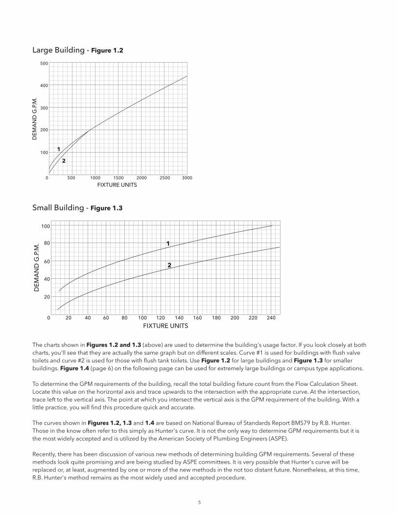
Large Building - Figure 1.2

Small Building - Figure 1.3

The charts shown in Figures 1.2 and 1.3 (above) are used to determine the building's usage factor. If you look closely at both charts, you'll see that they are actually the same graph but on different scales. Curve #1 is used for buildings with flush valve toilets and curve #2 is used for those with flush tank toilets. Use Figure 1.2 for large buildings and Figure 1.3 for smaller buildings. Figure 1.4 (page 6) on the following page can be used for extremely large buildings or campus type applications.

To determine the GPM requirements of the building, recall the total building fixture count from the Flow Calculation Sheet. Locate this value on the horizontal axis and trace upwards to the intersection with the appropriate curve. At the intersection, trace left to the vertical axis. The point at which you intersect the vertical axis is the GPM requirement of the building. With a little practice, you will find this procedure quick and accurate.

The curves shown in Figures 1.2, 1.3 and 1.4 are based on National Bureau of Standards Report BMS79 by R.B. Hunter. Those in the know often refer to this simply as Hunter's curve. It is not the only way to determine GPM requirements but it is the most widely accepted and is utilized by the American Society of Plumbing Engineers (ASPE).

Recently, there has been discussion of various new methods of determining building GPM requirements. Several of these methods look quite promising and are being studied by ASPE committees. It is very possible that Hunter's curve will be replaced or, at least, augmented by one or more of the new methods in the not too distant future. Nonetheless, at this time, R.B. Hunter's method remains as the most widely used and accepted procedure.

0 500 1000 1500 2000 2500 3000

1

2

100

500

200

300

400

FIXTURE UNITS

DE

MA

ND

G.P

.M.

0 20 40 60 80 100 120

100

80

20

40

60

FIXTURE UNITS

DE

MA

ND

G.P

.M. 1

2

140 160 180 200 220 240

6

0 5 10 15 20 25 30

10

20

30

FIXTURE UNITS (Thoudsands)

GPM

(Hun

dre

ds)

5

15

25

Multiple Large Buildings - Figure 1.4

7

SECTION 2DETERMINING BUILDING PRESSURE REQUIREMENTS HOW MUCH PRESSURE DOES MY BUILDING NEED?

Now that we know our GPM requirements, it is time to calculate the pressure boost required to maintain flow and pressure at all fixtures. Keep in mind that water, like people, tends to follow the path of least resistance. Therefore, if we satisfy the fixture at the end of the path of greatest resistance, it seems reasonable that we will satisfy all other fixtures in our system. When calculating this resistance, or pressure drop, it is important to totalize piping pressure drop and the pressure drop of the far-end fixture. The path of greatest pressure drop could be a long piping run to a unit with a very small pressure drop. Conversely, it may be a very short piping run to a unit with a very high pressure drop.

To calculate the pressure drop, we must take into account several factors including piping friction losses (including fittings), elevation of highest fixture and individual fixture pressure drop. While this can be a time consuming task, it is an important step in properly determining our final boost requirements. This publication includes several worksheets to assist you in maintaining records and performing the necessary calculations.

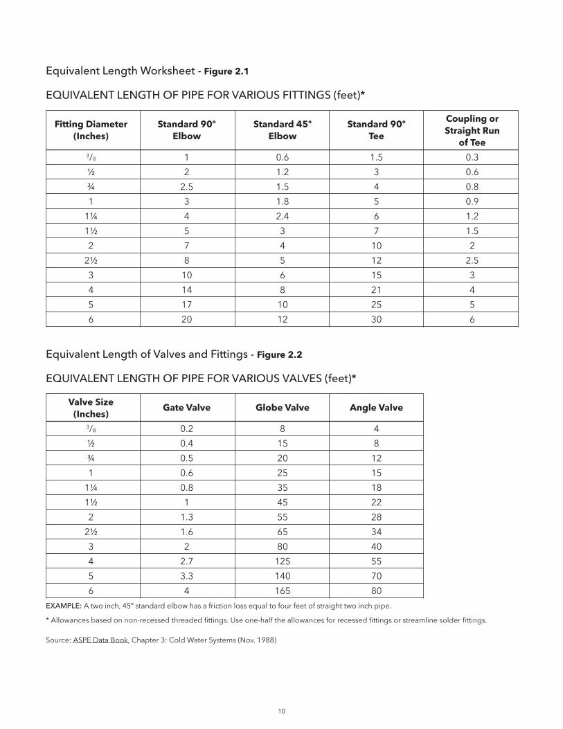
Our first step will be to determine the pressure drop across the various fittings (tees, ells, etc) in each piping branch. The worksheet and chart shown in Figures 2.1 (page 9) and 2.2 (page 10) respectively, will be our tools for this job. Step one is to trace the piping from the proposed booster location to the fixture at the farthest end of the piping branch. We must record the quantity of each type of fitting in column A of Figure 2.1 worksheet. Note that you will need one work sheet for each pipe size and flow rate in the piping run. After recording this data refer to the chart shown in Figure 2.2. This chart converts each fitting to an equivalent length of straight pipe. Record the equivalent length in the appropriate spaces in column B of Figure 2.1. After entering all data, multiply column A by column B and record your answer in column C. Add the figures in column C and move on to the next step.

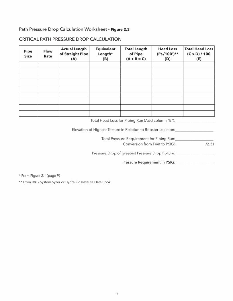
It is now time to determine the total pressure drop of the piping run. For this, we will use the path pressure drop worksheet shown in Figure 2.3 (page 11). You will also need a tool to determine pressure drop per 100' of pipe based on various flow rates. Ideally, you should use a Bell & Gossett System SyzerTM Calculator (Now available on computer disc). If you do not have this helpful tool, you can refer to the hydraulic Institute data book.

Record pipe size and flow rate in the first two columns. The actual length of straight pipe (less fittings) goes into column A. Record your total equivalent length of straight pipe (fittings only, from Figure 2.1) in column B. Remember that you will have a different value for each pipe size and flow rate. Now add columns A & B, record the sum in column C, Total Length of Pipe. Now refer to your System SyzerTM or Hydraulic Institute book to determine the pressure drop per 100’ of pipe for each size and GPM. Record this value in column D. After you have completed this exercise for the entire piping run, multiply column C by column D and divide by 100. Enter this value in column D. Now multiply column C by column D and divide the total by 100. Record the answer in column E. This is the total pressure drop for a pipe run of specific length, size and flow rate. Add the values in column E and record your answer in the appropriate space.

8

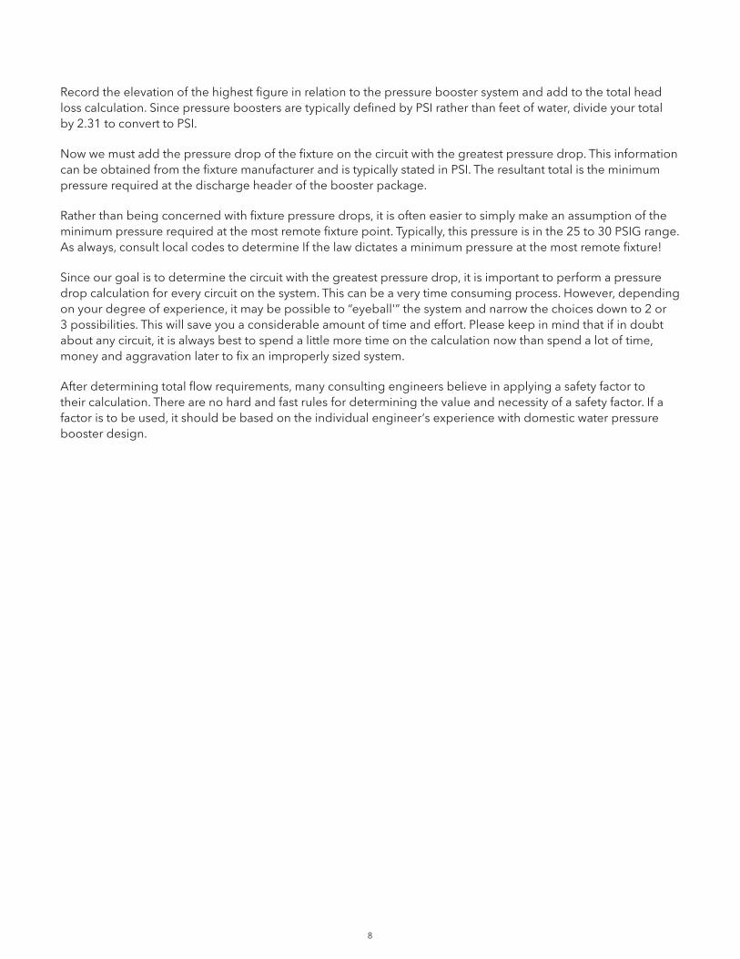
Record the elevation of the highest figure in relation to the pressure booster system and add to the total head loss calculation. Since pressure boosters are typically defined by PSI rather than feet of water, divide your total by 2.31 to convert to PSI.

Now we must add the pressure drop of the fixture on the circuit with the greatest pressure drop. This information can be obtained from the fixture manufacturer and is typically stated in PSI. The resultant total is the minimum pressure required at the discharge header of the booster package.

Rather than being concerned with fixture pressure drops, it is often easier to simply make an assumption of the minimum pressure required at the most remote fixture point. Typically, this pressure is in the 25 to 30 PSIG range. As always, consult local codes to determine If the law dictates a minimum pressure at the most remote fixture!

Since our goal is to determine the circuit with the greatest pressure drop, it is important to perform a pressure drop calculation for every circuit on the system. This can be a very time consuming process. However, depending on your degree of experience, it may be possible to “eyeball'” the system and narrow the choices down to 2 or 3 possibilities. This will save you a considerable amount of time and effort. Please keep in mind that if in doubt about any circuit, it is always best to spend a little more time on the calculation now than spend a lot of time, money and aggravation later to fix an improperly sized system.

After determining total flow requirements, many consulting engineers believe in applying a safety factor to their calculation. There are no hard and fast rules for determining the value and necessity of a safety factor. If a factor is to be used, it should be based on the individual engineer‘s experience with domestic water pressure booster design.

9

Equivalent Length Worksheet - Figure 2.1

EQUIVALENT LENGTHS OF STRAIGHT PIPE

PIPE SIZE: _______________________________________

FLOW RATE: _____________________________________

Valve/Fitting Type Quantity (A) Equivalent Length (B) Length of Straight Pipe AxB=(C)

Regular 90º ell

Long radius 90º ell

Regular 45º ell

Tee-line flow

Tee-branch flow

180º return bend

Globe valve

Gate valve

Angle valve

Swing check valve

Coupling or union

Total equivalent length of straight pipe (Add Column C) =__________________ ft.

10

Equivalent Length Worksheet - Figure 2.1

EQUIVALENT LENGTH OF PIPE FOR VARIOUS FITTINGS (feet)*

Fitting Diameter Standard 90º Standard 45º Standard 90º Coupling or (Inches) Elbow Elbow Tee Straight Run of Tee

3/8 1 0.6 1.5 0.3

½ 2 1.2 3 0.6

¾ 2.5 1.5 4 0.8

1 3 1.8 5 0.9

1¼ 4 2.4 6 1.2

1½ 5 3 7 1.5

2 7 4 10 2

2½ 8 5 12 2.5

3 10 6 15 3

4 14 8 21 4

5 17 10 25 5

6 20 12 30 6

Equivalent Length of Valves and Fittings - Figure 2.2

EQUIVALENT LENGTH OF PIPE FOR VARIOUS VALVES (feet)*

Valve Size Gate Valve Globe Valve Angle Valve (Inches)

3/8 0.2 8 4

½ 0.4 15 8

¾ 0.5 20 12

1 0.6 25 15

1¼ 0.8 35 18

1½ 1 45 22

2 1.3 55 28

2½ 1.6 65 34

3 2 80 40

4 2.7 125 55

5 3.3 140 70

6 4 165 80

EXAMPLE: A two inch, 45º standard elbow has a friction loss equal to four feet of straight two inch pipe.

* Allowances based on non-recessed threaded fittings. Use one-half the allowances for recessed fittings or streamline solder fittings.

Source: ASPE Data Book, Chapter 3: Cold Water Systems (Nov. 1988)

11

Path Pressure Drop Calculation Worksheet - Figure 2.3

CRITICAL PATH PRESSURE DROP CALCULATION

Pipe Flow Actual Length Equivalent Total Length Head Loss Total Head Loss Size Rate of Straight Pipe Length* of Pipe (Ft./100')** (C x D) / 100 (A) (B) (A + B = C) (D) (E)

Total Head Loss for Piping Run (Add column "E"):____________________

Elevation of Highest Texture in Relation to Booster Location:____________________

Total Pressure Requirement for Piping Run:____________________ Conversion from Feet to PSIG: /2.31

Pressure Drop of greatest Pressure Drop Fixture:____________________

Pressure Requirement in PSIG:____________________

* From Figure 2.1 (page 9)

** From B&G System Syzer or Hydraulic Institute Data Book

12

SUCTION PRESSURE CALCULATION

We have now determined the pressure required at the discharge of the booster. However, this is not actually what the package must generate. We need to look at our incoming or suction pressure. The required boost is equal to discharge pressure required less minimum available suction pressure. To calculate minimum suction pressure, refer to Figure 2.4, Suction Pressure Calculation Worksheet (page 13).

Minimum suction pressure at the city main can often be determined by contacting the local fire marshals or department of public works. If it is possible to simply measure the suction pressure at the point where the booster pump is to be installed, life is good. This will enable us to avoid another time consuming piping pressure drop calculation. Remember to always measure minimum suction pressure. That way, we can be sure that the folks on the top floor will be able to flush the toilet even when everybody in town is sprinkling their lawns.

Unless you are extremely fortunate, you will not have the luxury of taking a single gauge reading to determine minimum suction pressure. First we must measure the water pressure at a point as close to the booster pump suction as possible. The closer the point, the less piping calculations we'll have to perform. Record your measurement on line A of the Suction Pressure Calculation sheet. This is our gross minimum suction pressure. We will now subtract the negative effects on pressure to determine the net minimum suction pressure.

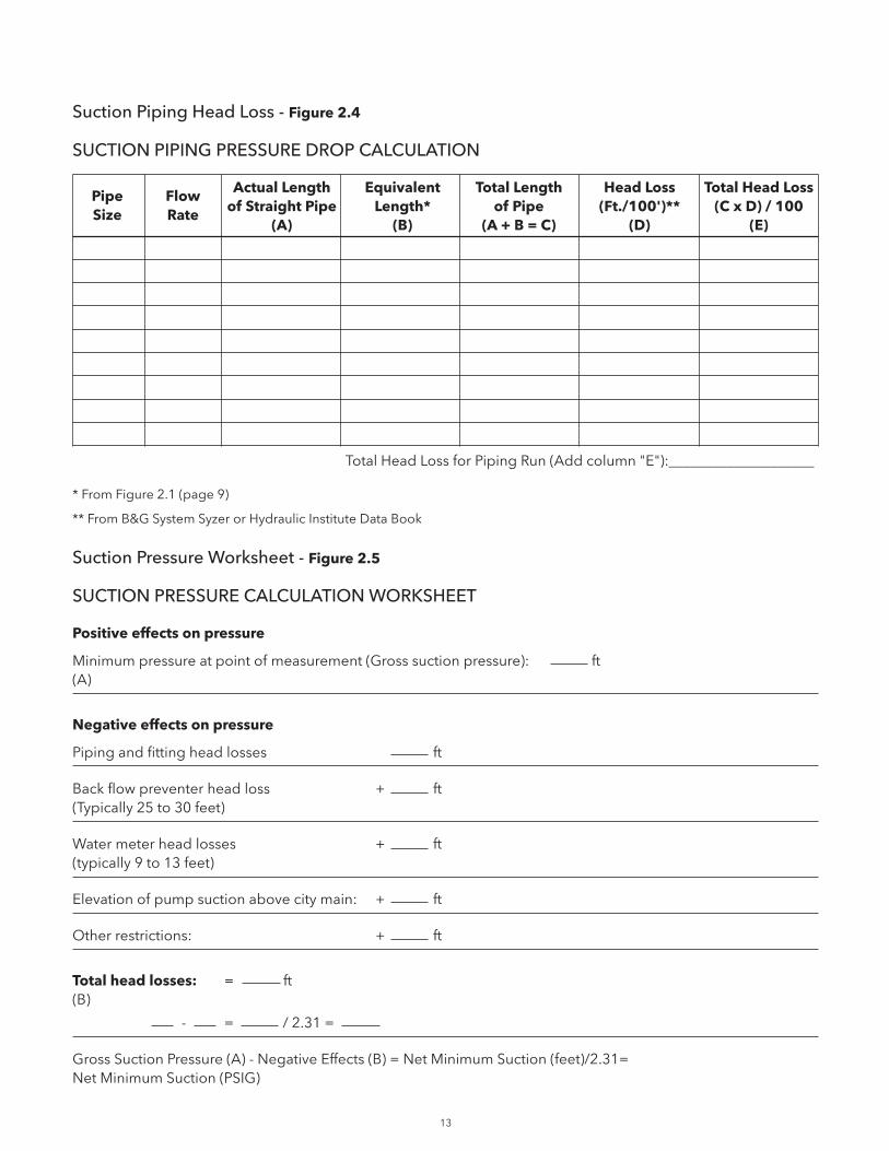
Refer back to the Equivalent Lengths Of Straight Pipe Worksheet in Figure 2.1. Trace the piping system from the point of pressure measurement to the booster pump suction. As before, note pipe sizes, flow rates and fitting types and sizes. Use the worksheet shown in Figure 2.4 to determine the piping pressure drop to the pump suction. Record this value as “piping and fitting pressure losses”. Your system will most likely have or require a back flow preventer (check local codes!) and water meter located between the city main and the pump suction. Record the pressure drop of these items in the appropriate spaces. Do not use estimates unless actual data is not available.

We must also add in the elevation (static height) of the pump suction above the city main and any other restrictions that do not fall into any of the previously mentioned categories. Record these values in the appropriate spaces.

Totalize the negative effects on suction pressure and record this value on line B. By subtracting line B from line A, we obtain the net minimum suction pressure available to our booster system. Divide this value by 2.31 to convert to PSIG.

13

Suction Piping Head Loss - Figure 2.4

SUCTION PIPING PRESSURE DROP CALCULATION

Pipe Flow Actual Length Equivalent Total Length Head Loss Total Head Loss Size Rate of Straight Pipe Length* of Pipe (Ft./100')** (C x D) / 100 (A) (B) (A + B = C) (D) (E)

Total Head Loss for Piping Run (Add column "E"):____________________

* From Figure 2.1 (page 9)

** From B&G System Syzer or Hydraulic Institute Data Book

Suction Pressure Worksheet - Figure 2.5

SUCTION PRESSURE CALCULATION WORKSHEET

Positive effects on pressure

Minimum pressure at point of measurement (Gross suction pressure): ft(A)

Negative effects on pressure

Piping and fitting head losses ft

Back flow preventer head loss + ft(Typically 25 to 30 feet)

Water meter head losses + ft(typically 9 to 13 feet)

Elevation of pump suction above city main: + ft

Other restrictions: + ft

Total head losses: = ft(B)

- = / 2.31 =

Gross Suction Pressure (A) - Negative Effects (B) = Net Minimum Suction (feet)/2.31= Net Minimum Suction (PSIG)

14

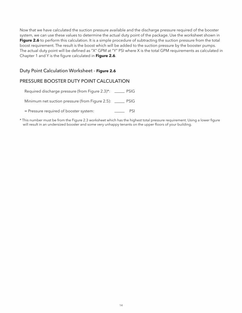
Now that we have calculated the suction pressure available and the discharge pressure required of the booster system, we can use these values to determine the actual duty point of the package. Use the worksheet shown in Figure 2.6 to perform this calculation. It is a simple procedure of subtracting the suction pressure from the total boost requirement. The result is the boost which will be added to the suction pressure by the booster pumps. The actual duty point will be defined as “X” GPM at “Y” PSI where X is the total GPM requirements as calculated in Chapter 1 and Y is the figure calculated in Figure 2.6.

Duty Point Calculation Worksheet - Figure 2.6

PRESSURE BOOSTER DUTY POINT CALCULATION

Required discharge pressure (from Figure 2.3)*: PSIG

Minimum net suction pressure (from Figure 2.5): PSIG

= Pressure required of booster system: PSI

* This number must be from the Figure 2.3 worksheet which has the highest total pressure requirement. Using a lower figure will result in an undersized booster and some very unhappy tenants on the upper floors of your building.

15

SECTION 3DOMESTIC WATER PIPE SIZING

The first step in sizing domestic water pipe is to determine the individual flow requirements of both hot and cold water. We will also need to recall the total system GPM as calculated in Section 1.

Below are Figures 3.1 and 3.2 from Section 1. By calculating the fixture unit counts for hot and cold water, we can determine the GPM requirements. These figures will then be used to determine pipe size.

Large Building - Figure 3.1

Small Building - Figure 3.2

Use curve 1 for cold water flow estimation when using flush valve toilets. Use curve 2 for hot water flow estimation and cold water flow estimation when using flush tank toilets.

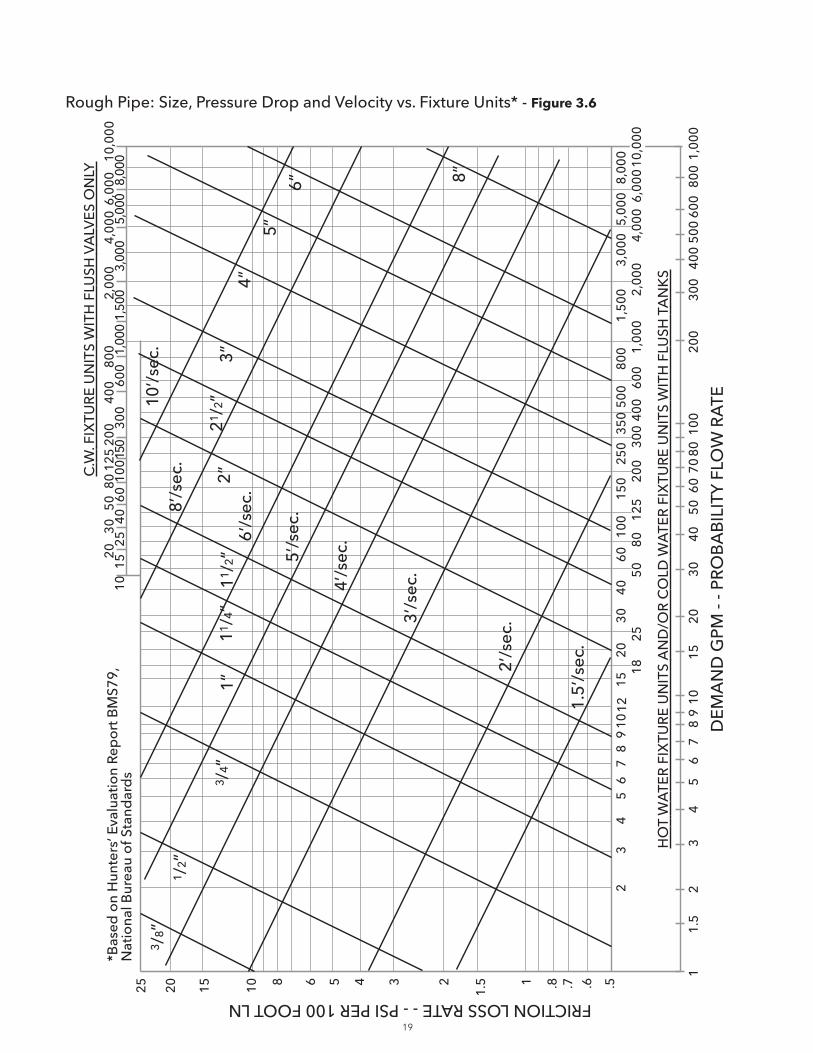
The flow requirements we establish from fixture unit counts is related to pipe size by pressure drop and flow velocity considerations. The relationship is categorized by the type of pipe being used. Our good friend R.B. Hunter from Section 1 broke piping into four different groups: “smooth copper tube”, “fairly smooth galvanized”, “fairly rough galvanized” and “rough galvanized”. Bell & Gossett has merged Hunter's data into the graphs shown in Figures 3.3, 3.4, 3.5, and 3.6. These graphs represent the correlation of fixture units to pipe size, pressure drop, velocity and demand flow rate. The graphs illustrate these relationships in smooth copper tubing, fairly smooth, fairly rough and rough galvanized pipe.

0 500 1000 1500 2000 2500 3000

1

2

100

500

200

300

400

FIXTURE UNITS

DE

MA

ND

G.P

.M.

0 20 40 60 80 100 120

100

80

20

40

60

FIXTURE UNITS

DE

MA

ND

G.P

.M. 1

2

140 160 180 200 220 240

16

Copper Tubing: Size, Pressure Drop and Velocity vs. Fixture Units* - Figure 3.3

11.

5

.5.6

DE

MA

ND

GPM

- - P

RO

BA

BIL

ITY

FLO

W R

ATE

FRICTION LOSS RATE - - PSI PER 100 FOOT LN

23

45

67

89

1015

2030

4050

6070

8010

020

030

040

050

060

080

01,

000

HO

T W

ATE

R F

IXTU

RE

UN

ITS

AN

D/O

R C

OLD

WA

TER

FIX

TUR

E U

NIT

S W

ITH

FLU

SH T

AN

KS

.81 .71.523456810152025

23

45

67

89

1012

1815

2030

4025

5060

100

150

250

8012

520

030

040

035

050

080

060

01,

0001,

500 2,

0003,

000 4,

000

5,00

08,

000

6,00

010

,000

2030

5080

125

200

400

800

2,00

04,

000

6,00

010

,000

1015

2540

6010

015

030

060

01,

000

1,50

03,

000

5,00

08,

000

C.W

. FIX

TUR

E U

NIT

S W

ITH

FLU

SH V

ALV

ES

ON

LY

*Bas

ed o

n H

unte

rs’ E

valu

atio

n Re

po

rt B

MS7

9,N

atio

nal B

urea

u o

f Sta

ndar

ds

3 /8”

KL M

1 /2”

L MK

3 /4”

KML 1”

KML

11/ 4

”11

/2”

21/2

”

2”

3”

4”

5”

6”

2’/s

ec.3’

/sec

.

4’/s

ec.

5’/s

ec.

6’/

sec.

8’/s

ec.

10’/

sec.15

’/se

c.

17

Fairly Smooth Pipe: Size, Pressure Drop and Velocity vs. Fixture Units* - Figure 3.4

11.

5

.5.6

DE

MA

ND

GPM

- - P

RO

BA

BIL

ITY

FLO

W R

ATE

FRICTION LOSS RATE - - PSI PER 100 FOOT LN

23

45

67

89

1015

2030

4050

6070

8010

020

030

040

050

060

080

01,

000

HO

T W

ATE

R F

IXTU

RE

UN

ITS

AN

D/O

R C

OLD

WA

TER

FIX

TUR

E U

NIT

S W

ITH

FLU

SH T

AN

KS

.81 .71.523456810152025

23

45

67

89

1012

1815

2030

4025

5060

100

150

250

8012

520

030

040

035

050

080

060

01,

0001,

500 2,

0003,

000 4,

000

5,00

08,

000

6,00

010

,000

2030

5080

125

200

400

800

2,00

04,

000

6,00

010

,000

1015

2540

6010

015

030

060

01,

000

1,50

03,

000

5,00

08,

000

C.W

. FIX

TUR

E U

NIT

S W

ITH

FLU

SH V

ALV

ES

ON

LY

*Bas

ed o

n H

unte

rs’ E

valu

atio

n Re

po

rt B

MS7

9,N

atio

nal B

urea

u o

f Sta

ndar

ds

3 /8”

1 /2 ”

3 /4”

1”11

/4”

11/2

”21

/ 2”

2”

3”

4”

5”

6”

2’/s

ec.3’

/sec

.

4’/s

ec.

5’/s

ec.

6’/s

ec.8’/s

ec.

10’/

sec.

15’/

sec.

18

Fairly Rough Pipe: Size, Pressure Drop and Velocity vs. Fixture Units* - Figure 3.5

11.

5

.5.6

DE

MA

ND

GPM

- - P

RO

BA

BIL

ITY

FLO

W R

ATE

FRICTION LOSS RATE - - PSI PER 100 FOOT LN

23

45

67

89

1015

2030

4050

6070

8010

020

030

040

050

060

080

01,

000

HO

T W

ATE

R F

IXTU

RE

UN

ITS

AN

D/O

R C

OLD

WA

TER

FIX

TUR

E U

NIT

S W

ITH

FLU

SH T

AN

KS

.81 .71.523456810152025

23

45

67

89

1012

1815

2030

4025

5060

100

150

250

8012

520

030

040

035

050

080

060

01,

0001,

500 2,

0003,

000 4,

000

5,00

08,

000

6,00

010

,000

2030

5080

125

200

400

800

2,00

04,

000

6,00

010

,000

1015

2540

6010

015

030

060

01,

000

1,50

03,

000

5,00

08,

000

C.W

. FIX

TUR

E U

NIT

S W

ITH

FLU

SH V

ALV

ES

ON

LY

*Bas

ed o

n H

unte

rs’ E

valu

atio

n Re

po

rt B

MS7

9,N

atio

nal B

urea

u o

f Sta

ndar

ds

3 /8”

1 /2”

3 /4”

1”11

/4”

11/2

”21

/ 2”

2”3”

4”5” 6”

2’/s

ec.3’

/sec

.4’/s

ec.

5’/s

ec.

6’/s

ec.

8’/s

ec.

10’/

sec.

8”

19

Rough Pipe: Size, Pressure Drop and Velocity vs. Fixture Units* - Figure 3.6

11.

5

.5.6

DE

MA

ND

GPM

- - P

RO

BA

BIL

ITY

FLO

W R

ATE

FRICTION LOSS RATE - - PSI PER 100 FOOT LN

23

45

67

89

1015

2030

4050

6070

8010

020

030

040

050

060

080

01,

000

HO

T W

ATE

R F

IXTU

RE

UN

ITS

AN

D/O

R C

OLD

WA

TER

FIX

TUR

E U

NIT

S W

ITH

FLU

SH T

AN

KS

.81 .71.523456810152025

23

45

67

89

1012

1815

2030

4025

5060

100

150

250

8012

520

030

040

035

050

080

060

01,

0001,

500 2,

0003,

000 4,

000

5,00

08,

000

6,00

010

,000

2030

5080

125

200

400

800

2,00

04,

000

6,00

010

,000

1015

2540

6010

015

030

060

01,

000

1,50

03,

000

5,00

08,

000

C.W

. FIX

TUR

E U

NIT

S W

ITH

FLU

SH V

ALV

ES

ON

LY

*Bas

ed o

n H

unte

rs’ E

valu

atio

n Re

po

rt B

MS7

9,N

atio

nal B

urea

u o

f Sta

ndar

ds

3 /8”

1 /2”

3 /4”

1”11

/4”

11/2

”21

/2”

2”3”

4”5”

6”

2’/s

ec.3’

/sec

.

4’/s

ec.

5’/s

ec.

6’/s

ec.

8’/s

ec.

10’/

sec.

8”

1.5’

/sec

.

20

Since this data is based on Hunter's probability curves and friction loss curves, it is generally believed that pipe sized by this method tends to be oversized. However, it was Hunter's intent to provide a safety factor in this calculation. Since the rate of pipe tuberculation is still an undefined variable, this safety factor ensures that we do not end up with undersized pipe.

Most designers establish limitations on maximum allowable friction loss rate and/or maximum velocity when designing domestic water systems. High velocities can cause unacceptable levels of flow noise. Excessive piping pressure drops can have an adverse effect on hot and cold water flow mixing stability.

Design limitations vary and we should always consult the local building code before determining the limitations we are going to use. Some of the more common criteria are as follows:

1. Use of an across the board pressure drop limitation. In this case, we simply size pipe based on a maximum allowable pressure drop per length of pipe. This pressure drop is usually set at 5 PSI per 100’. We will not be concerned with velocity.

2. Use of a 5 PSI per 100’ pressure drop limitation without exceeding a velocity of 8 feet per second.

3. Use of a velocity limitation only. Common limitations are in the 6 to 10 feet per second range.

These approaches have all worked satisfactorily due to the safety factor built into the probability flow demand statements and conservative estimates of pipe corrosion. As a rule, however, numbers 1 & 2 tend to result in lower levels of velocity noise adjacent to occupied spaces.

The suggested 5 PSI per 100’ may seem high when compared to the 1.75 PSI (4’) per 100’ we generally see in hydronic design. However, keep in mind that with a domestic water system, we are looking at a probability flow vs. a set defined flow for hydronic systems.

The basic problems associated with flow noise and hot - cold flow ratio mix must be carefully evaluated before riser pipe sizes are reduced. The cost saving we achieve by using 1” pipe instead of 1.25”. pipe can be quickly nullified when you realize that we are increasing the pressure drop by a factor of nearly four.

Pipe sizing to Hunter's probability curves and pipe sizing charts work well providing that reasonable sizing limitations are used. A conservative, yet reasonable limitation is the across the board 5 PSIG per 100’ maximum friction loss rate. Always bear in mind that, due to the many unknowns, your criteria is a matter of individual judgment based on learning and experience.

Pipe sizing tables further simplify design work and can be easily established from the fixture unit/pipe sizing chart correlation for friction loss rate or velocity parameters.

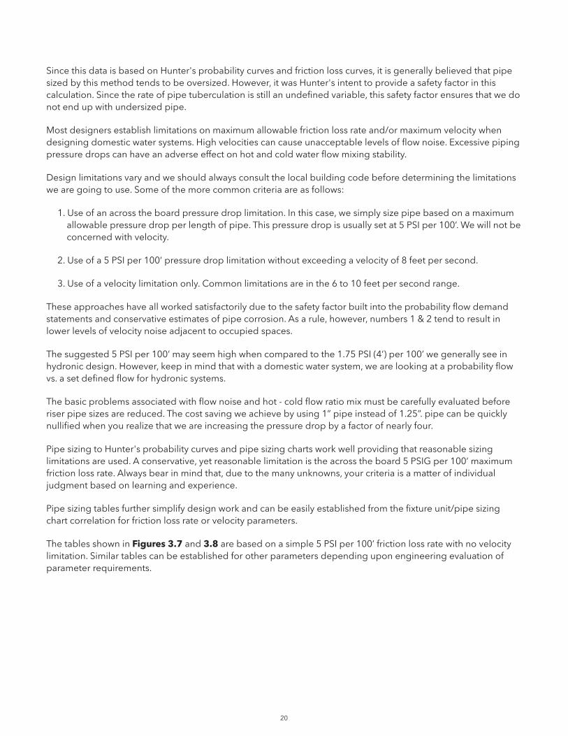
The tables shown in Figures 3.7 and 3.8 are based on a simple 5 PSI per 100’ friction loss rate with no velocity limitation. Similar tables can be established for other parameters depending upon engineering evaluation of parameter requirements.

21

Fairly Smooth Pipe - Figure 3.7

MAXIMUM FLOW DEMAND / FIXTURE COUNT @ 5 PSI / 100’ FRICTION LOSS WITH COPPER TUBING

No. Fixture Units GPM Copper Tube Size (Inches) No. Fixture Units (Flush Tank)* Demand Based on 5 PSI / 100' Pressure Loss (Flush Valve)**

0-2 0-2.1 0.5 ***

2.5-7.5 2.1-6.2 0.75 ***

7.5-18 6.2-13 1 ***

18-36 13-23 1.25 ***

36-70 23-35 1.5 10-28

70-240 35-75 2 28-130

240-575 75-140 2.5 130-500

575-1200 140-230 3 500-1200

1200-4000 230-520 4 1200-4000

Rough Pipe - Figure 3.8

MAXIMUM FLOW DEMAND / FIXTURE COUNT @ 5 PSI / 100’ FRICTION LOSS WITH ROUGH PIPE

No. Fixture Units GPM Rough Pipe Size (Inches) No. Fixture Units (Flush Tank)* Demand Based on 5 PSI / 100' Pressure Loss (Flush Valve)**

0-1 0-1.5 0.5 ***

1-4.5 1.5-4 .075 ***

4.5-11 4-8.5 1 ***

11-20 8.5-15 1.25 ***

20-35 15-23 1.5 ***

35-120 23-46 2 10-42

120-275 46-85 2.5 42-170

275-520 85-130 3 170-400

520-1400 130-260 4 400-1400

1400-3200 260-450 5 1400-3200

3200-6200 450-720 6 3200-6200

* Always applies to hot water distribution

** Should be confirmed by flush valve manufacturer

*** Consult flush valve manufacturer.

22

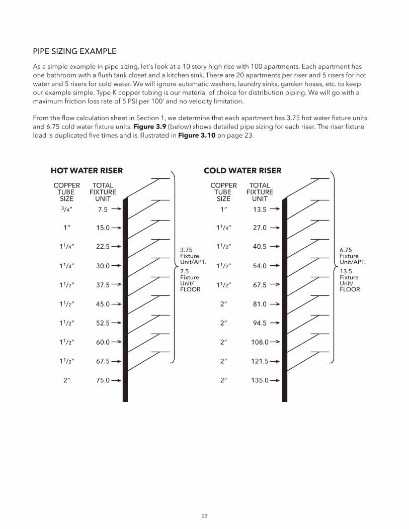
PIPE SIZING EXAMPLE

As a simple example in pipe sizing, let's look at a 10 story high rise with 100 apartments. Each apartment has one bathroom with a flush tank closet and a kitchen sink. There are 20 apartments per riser and 5 risers for hot water and 5 risers for cold water. We will ignore automatic washers, laundry sinks, garden hoses, etc. to keep our example simple. Type K copper tubing is our material of choice for distribution piping. We will go with a maximum friction loss rate of 5 PSI per 100’ and no velocity limitation.

From the flow calculation sheet in Section 1, we determine that each apartment has 3.75 hot water fixture units and 6.75 cold water fixture units. Figure 3.9 (below) shows detailed pipe sizing for each riser. The riser fixture load is duplicated five times and is illustrated in Figure 3.10 on page 23.

COLD WATER RISER

COPPER TOTALTUBE FIXTURESIZE UNIT3/4” 7.5

1” 15.0

11/4” 22.5

11/4” 30.0

11/2” 37.5

11/2” 45.0

11/2” 52.5

11/2” 60.0

11/2” 67.5

2” 75.0

HOT WATER RISER

3.75FixtureUnit/APT.

7.5FixtureUnit/FLOOR

COPPER TOTALTUBE FIXTURESIZE UNIT

1” 13.5

11/4” 27.0

11/2” 40.5

11/2” 54.0

11/2” 67.5

2” 81.0

2” 94.5

2” 108.0

2” 121.5

2” 135.0

6.75FixtureUnit/APT.

13.5FixtureUnit/FLOOR

23

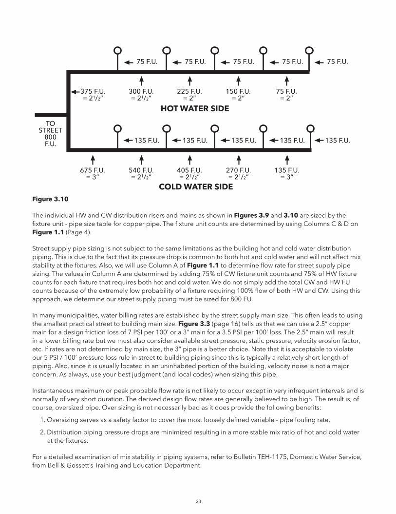
Figure 3.10

The individual HW and CW distribution risers and mains as shown in Figures 3.9 and 3.10 are sized by the fixture unit - pipe size table for copper pipe. The fixture unit counts are determined by using Columns C & D on Figure 1.1 (Page 4).

Street supply pipe sizing is not subject to the same limitations as the building hot and cold water distribution piping. This is due to the fact that its pressure drop is common to both hot and cold water and will not affect mix stability at the fixtures. Also, we will use Column A of Figure 1.1 to determine flow rate for street supply pipe sizing. The values in Column A are determined by adding 75% of CW fixture unit counts and 75% of HW fixture counts for each fixture that requires both hot and cold water. We do not simply add the total CW and HW FU counts because of the extremely low probability of a fixture requiring 100% flow of both HW and CW. Using this approach, we determine our street supply piping must be sized for 800 FU.

In many municipalities, water billing rates are established by the street supply main size. This often leads to using the smallest practical street to building main size. Figure 3.3 (page 16) tells us that we can use a 2.5” copper main for a design friction loss of 7 PSI per 100’ or a 3” main for a 3.5 PSI per 100’ loss. The 2.5” main will result in a lower billing rate but we must also consider available street pressure, static pressure, velocity erosion factor, etc. If rates are not determined by main size, the 3” pipe is a better choice. Note that it is acceptable to violate our 5 PSI / 100’ pressure loss rule in street to building piping since this is typically a relatively short length of piping. Also, since it is usually located in an uninhabited portion of the building, velocity noise is not a major concern. As always, use your best judgment (and local codes) when sizing this pipe.

Instantaneous maximum or peak probable flow rate is not likely to occur except in very infrequent intervals and is normally of very short duration. The derived design flow rates are generally believed to be high. The result is, of course, oversized pipe. Over sizing is not necessarily bad as it does provide the following benefits:

1. Oversizing serves as a safety factor to cover the most loosely defined variable - pipe fouling rate.

2. Distribution piping pressure drops are minimized resulting in a more stable mix ratio of hot and cold water at the fixtures.

For a detailed examination of mix stability in piping systems, refer to Bulletin TEH-1175, Domestic Water Service, from Bell & Gossett’s Training and Education Department.

COLD WATER SIDE

75 F.U.

HOT WATER SIDE

75 F.U.75 F.U.75 F.U.75 F.U.

135 F.U.135 F.U.135 F.U.135 F.U.135 F.U.

75 F.U.= 2”

150 F.U.= 2”

225 F.U.= 2”

300 F.U.= 21/2”

375 F.U.= 21/2”

TOSTREET

800F.U.

540 F.U.= 21/2”

405 F.U.= 21/2”

270 F.U.= 21/2”

135 F.U.= 3”

675 F.U.= 3”

24

SECTION 4PRESSURE BOOSTER SELECTION PROCEDURE

SYSTEM SPLITS

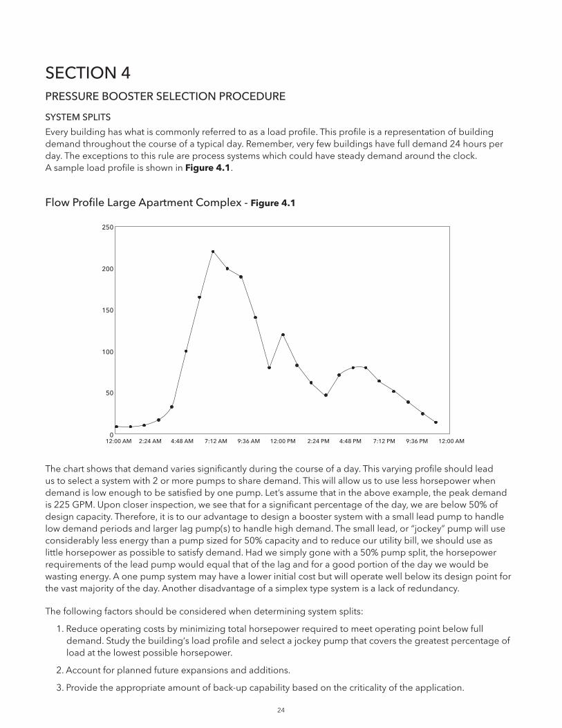
Every building has what is commonly referred to as a load profile. This profile is a representation of building demand throughout the course of a typical day. Remember, very few buildings have full demand 24 hours per day. The exceptions to this rule are process systems which could have steady demand around the clock. A sample load profile is shown in Figure 4.1.

Flow Profile Large Apartment Complex - Figure 4.1

The chart shows that demand varies significantly during the course of a day. This varying profile should lead us to select a system with 2 or more pumps to share demand. This will allow us to use less horsepower when demand is low enough to be satisfied by one pump. Let’s assume that in the above example, the peak demand is 225 GPM. Upon closer inspection, we see that for a significant percentage of the day, we are below 50% of design capacity. Therefore, it is to our advantage to design a booster system with a small lead pump to handle low demand periods and larger lag pump(s) to handle high demand. The small lead, or “jockey” pump will use considerably less energy than a pump sized for 50% capacity and to reduce our utility bill, we should use as little horsepower as possible to satisfy demand. Had we simply gone with a 50% pump split, the horsepower requirements of the lead pump would equal that of the lag and for a good portion of the day we would be wasting energy. A one pump system may have a lower initial cost but will operate well below its design point for the vast majority of the day. Another disadvantage of a simplex type system is a lack of redundancy.

The following factors should be considered when determining system splits:

1. Reduce operating costs by minimizing total horsepower required to meet operating point below full demand. Study the building‘s load profile and select a jockey pump that covers the greatest percentage of load at the lowest possible horsepower.

2. Account for planned future expansions and additions.

3. Provide the appropriate amount of back-up capability based on the criticality of the application.

0

50

100

150

200

250

12:00 AM 2:24 AM 4:48 AM 7:12 AM 9:36 AM 12:00 PM 2:24 PM 4:48 PM 7:12 PM 9:36 PM 12:00 AM

25

PRESSURE BOOSTER PACKAGE LOSS CALCULATION

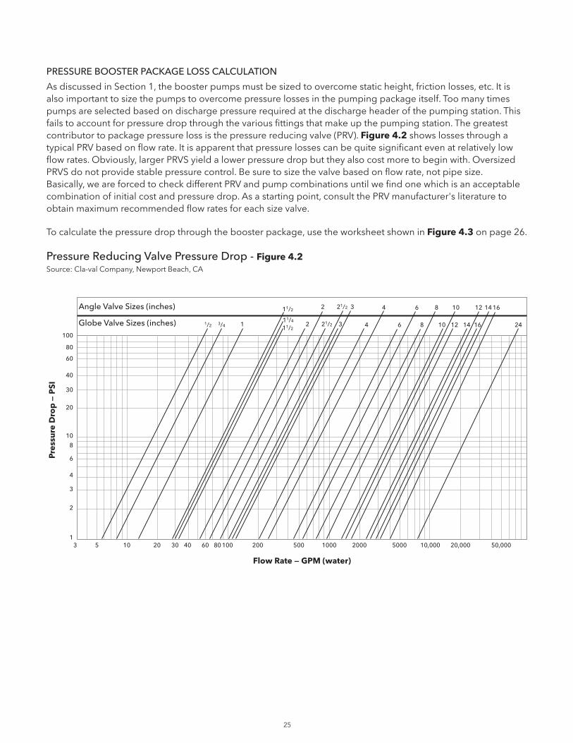
As discussed in Section 1, the booster pumps must be sized to overcome static height, friction losses, etc. It is also important to size the pumps to overcome pressure losses in the pumping package itself. Too many times pumps are selected based on discharge pressure required at the discharge header of the pumping station. This fails to account for pressure drop through the various fittings that make up the pumping station. The greatest contributor to package pressure loss is the pressure reducing valve (PRV). Figure 4.2 shows losses through a typical PRV based on flow rate. It is apparent that pressure losses can be quite significant even at relatively low flow rates. Obviously, larger PRVS yield a lower pressure drop but they also cost more to begin with. Oversized PRVS do not provide stable pressure control. Be sure to size the valve based on flow rate, not pipe size. Basically, we are forced to check different PRV and pump combinations until we find one which is an acceptable combination of initial cost and pressure drop. As a starting point, consult the PRV manufacturer's literature to obtain maximum recommended flow rates for each size valve.

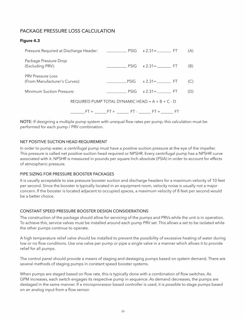
To calculate the pressure drop through the booster package, use the worksheet shown in Figure 4.3 on page 26.

Pressure Reducing Valve Pressure Drop - Figure 4.2Source: Cla-val Company, Newport Beach, CA

1

Angle Valve Sizes (inches)

Globe Valve Sizes (inches)

2

3

4

6

8

10

20

30

40

60

80

100

3 5 10 20 30 40 60 80 100 200 500 1000 2000 5000 10,000 20,000 50,000

Flow Rate — GPM (water)

Pres

sure

Dro

p —

PSI

1/2 3/4 1 2 3 4 6 8 10 12 14 16 24

2 3 4 6 8 10 12 14 1611/2

11/4

11/221/2

21/2

26

PACKAGE PRESSURE LOSS CALCULATION

Figure 4.3

Pressure Required at Discharge Header: __________ PSIG x 2.31= _______ FT (A)

Package Pressure Drop(Excluding PRV): __________ PSIG x 2.31= _______ FT (B)

PRV Pressure Loss(From Manufacturer's Curves): __________PSIG x 2.31= _______ FT (C)

Minimum Suction Pressure: __________ PSIG x 2.31= _______ FT (D)

REQUIRED PUMP TOTAL DYNAMIC HEAD = A + B + C - D

_______ FT + ______FT + ______ FT - ______ FT = ______ FT

NOTE: If designing a multiple pump system with unequal flow rates per pump, this calculation must be performed for each pump / PRV combination.

NET POSITIVE SUCTION HEAD REQUIREMENT

In order to pump water, a centrifugal pump must have a positive suction pressure at the eye of the impeller. This pressure is called net positive suction head required or NPSHR. Every centrifugal pump has a NPSHR curve associated with it. NPSHR is measured in pounds per square Inch absolute (PSIA) in order to account for effects of atmospheric pressure.

PIPE SIZING FOR PRESSURE BOOSTER PACKAGES

It is usually acceptable to size pressure booster suction and discharge headers for a maximum velocity of 10 feet per second. Since the booster is typically located in an equipment room, velocity noise is usually not a major concern. If the booster is located adjacent to occupied spaces, a maximum velocity of 8 feet per second would be a better choice.

CONSTANT SPEED PRESSURE BOOSTER DESIGN CONSIDERATIONS

The construction of the package should allow for servicing of the pumps and PRVs while the unit is in operation. To achieve this, service valves must be installed around each pump PRV set. This allows a set to be isolated while the other pumps continue to operate.

A high temperature relief valve should be installed to prevent the possibility of excessive heating of water during low or no flow conditions. Use one valve per pump or pipe a single valve in a manner which allows it to provide relief for all pumps.

The control panel should provide a means of staging and destaging pumps based on system demand. There are several methods of staging pumps in constant speed booster systems.

When pumps are staged based on flow rate, this is typically done with a combination of flow switches. As GPM increases, each switch engages its respective pump in sequence. As demand decreases, the pumps are destaged in the same manner. If a microprocessor based controller is used, it is possible to stage pumps based on an analog input from a flow sensor.

27

Pumps can also be staged based on pressure. Similar to flow staging, as the pressure switch senses a loss in system pressure, it engages the next pump in sequence. As with flow staging, it is possible for a microprocessor based controller to use a pressure sensor instead of switches.

At this time, the most common method of pump staging is based on current. Current sensing relays are used to determine where the pump is operating on its curve. As the pump moves out to the right, the motor will draw more amps. At a preset point, the current relay trips and engages the next pump in sequence. The advantage of this type of staging is that there are no moving parts to wear out or clog up.

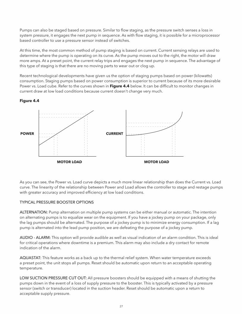
Recent technological developments have given us the option of staging pumps based on power (kilowatts) consumption. Staging pumps based on power consumption is superior to current because of its more desirable Power vs. Load cube. Refer to the curves shown in Figure 4.4 below. It can be difficult to monitor changes in current draw at low load conditions because current doesn't change very much.

Figure 4.4

As you can see, the Power vs. Load curve depicts a much more linear relationship than does the Current vs. Load curve. The linearity of the relationship between Power and Load allows the controller to stage and restage pumps with greater accuracy and improved efficiency at low load conditions.

TYPICAL PRESSURE BOOSTER OPTIONS

ALTERNATION: Pump alternation on multiple pump systems can be either manual or automatic. The intention on alternating pumps is to equalize wear on the equipment. If you have a jockey pump on your package, only the lag pumps should be alternated. The purpose of a jockey pump is to minimize energy consumption. If a lag pump is alternated into the lead pump position, we are defeating the purpose of a jockey pump.

AUDIO - ALARM: This option will provide audible as well as visual indication of an alarm condition. This is ideal for critical operations where downtime is a premium. This alarm may also include a dry contact for remote indication of the alarm.

AQUASTAT: This feature works as a back up to the thermal relief system. When water temperature exceeds a preset point, the unit stops all pumps. Reset should be automatic upon return to an acceptable operating temperature.

LOW SUCTION PRESSURE CUT OUT: AII pressure boosters should be equipped with a means of shutting the pumps down in the event of a loss of supply pressure to the booster. This is typically activated by a pressure sensor (switch or transducer) located in the suction header. Reset should be automatic upon a return to acceptable supply pressure.

POWER

MOTOR LOAD

CURRENT

MOTOR LOAD

28

LOW WATER LEVEL CUT OUT: When pumping out of a tank or cistern, this option will shut the system down if tank level drops below an acceptable point. When level is once again acceptable, the system is restarted.

HIGH SUCTION PRESSURE CUT OUT: This option will shut the pumps down when city supply pressure is high enough to satisfy the demand without requiring additional boost.

NO FLOW SHUT DOWN: During periods of low or no demand, we can save additional energy by stopping the pumps with this feature. A hydropneumatic tank should always be used with no flow shut down to satisfy minimal demand on the system and keep the pumps off for a reasonable amount of time. See Section 5 for further details on hydropneumatic tanks.

FUSED DISCONNECT / CIRCUIT BREAKERS: This gives maintenance personnel a means to shut down the system and provides individual short circuit protection for each motor. This option may assure you meet NEC requirements of having a disconnect switch located in sight of the motor. Consult latest revision of NEC handbook for details.

FLOW READ-OUT: In certain applications, it may be desirable to display instantaneous flow rate in gallons per minute. This is typically accomplished by installing a flow transmitter somewhere in the discharge main prior to any branches. This transmitter sends a 4-20 mA signal back to the pressure booster control panel for the GPM display.

MATERIALS OF CONSTRUCTION

Materials of construction are normally dictated by the type of water being pumped and the processes to which the water is being pumped. Many municipalities have codes requiring certain materials for domestic water service. The most common header materials are copper and galvanized steel. Stainless steel is used in many food processing plants.

SECTION 5HYDROPNEUMATIC TANK SIZING

Hydropneumatic tanks are primarily used in a domestic water system for draw down purposes when the pressure booster system is off on no-flow shutdown (NFSD). The NFSD circuitry turns the lead pump off when there is no demand on the system. While the system is off in this condition, the hydropneumatic tank will satisfy small demands on the system. Without the tank, the booster would restart upon the slightest call for flow such as a single toilet being flushed or even a minute leak in the piping system.

Hydropneumatic tank sizing is dependent on two factors:

1. Length of time you wish the pumps to remain off in a no-flow situation.

2. The tank location in relation to the pressure booster.

Any given building will have a low demand rate for various times of the day. Leaky faucets or someone getting a glass of water in the middle of the night are factors which prevent this low demand period from being a no demand period. It is not often that a system will have periods of zero demand.

The estimated low demand GPM should be multiplied by the minimum number of minutes you want your booster to stay off on no-flow shutdown to determine draw down volume of the tank. Due to the time delays built into most no-flow shutdown circuits, three minutes is generally the minimum off time considered. Typically, the maximum amount of time is 30 minutes. The longer the unit is off the more energy we save but the larger our tank must be. Therefore, a compromise must be made between tank size and minimum shutdown time.

29

TANK DRAW DOWN CALCULATION

The tank size is not equal to the amount of water which can actually be drawn from the tank. The usable volume of the tank is dependent upon the normal system pressure, minimum allowable system pressure and the drawdown coefficient of the tank. This drawdown coefficient can be obtained from the tank manufacturer's published data.

HYDROPNEUMATIC TANK PLACEMENT

There are several places where a hydropneumatic tank can be connected to the system. The most common connection point is to the discharge header of the booster package. Some tanks are connected just after the discharge of the pump but before the PRV. Another fairly common location is farther out in the system, usually on the roof of the building. There are pros and cons to each location.

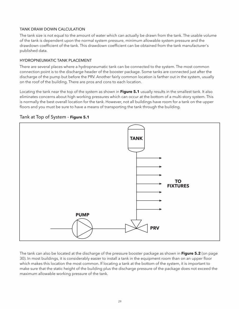
Locating the tank near the top of the system as shown in Figure 5.1 usually results in the smallest tank. It also eliminates concerns about high working pressures which can occur at the bottom of a multi-story system. This is normally the best overall location for the tank. However, not all buildings have room for a tank on the upper floors and you must be sure to have a means of transporting the tank through the building.

Tank at Top of System - Figure 5.1

The tank can also be located at the discharge of the pressure booster package as shown in Figure 5.2 (on page 30). In most buildings, it is considerably easier to install a tank in the equipment room than on an upper floor which makes this location the most common. If locating a tank at the bottom of the system, it is important to make sure that the static height of the building plus the discharge pressure of the package does not exceed the maximum allowable working pressure of the tank.

PUMP

PRV

TANK

TOFIXTURES

30

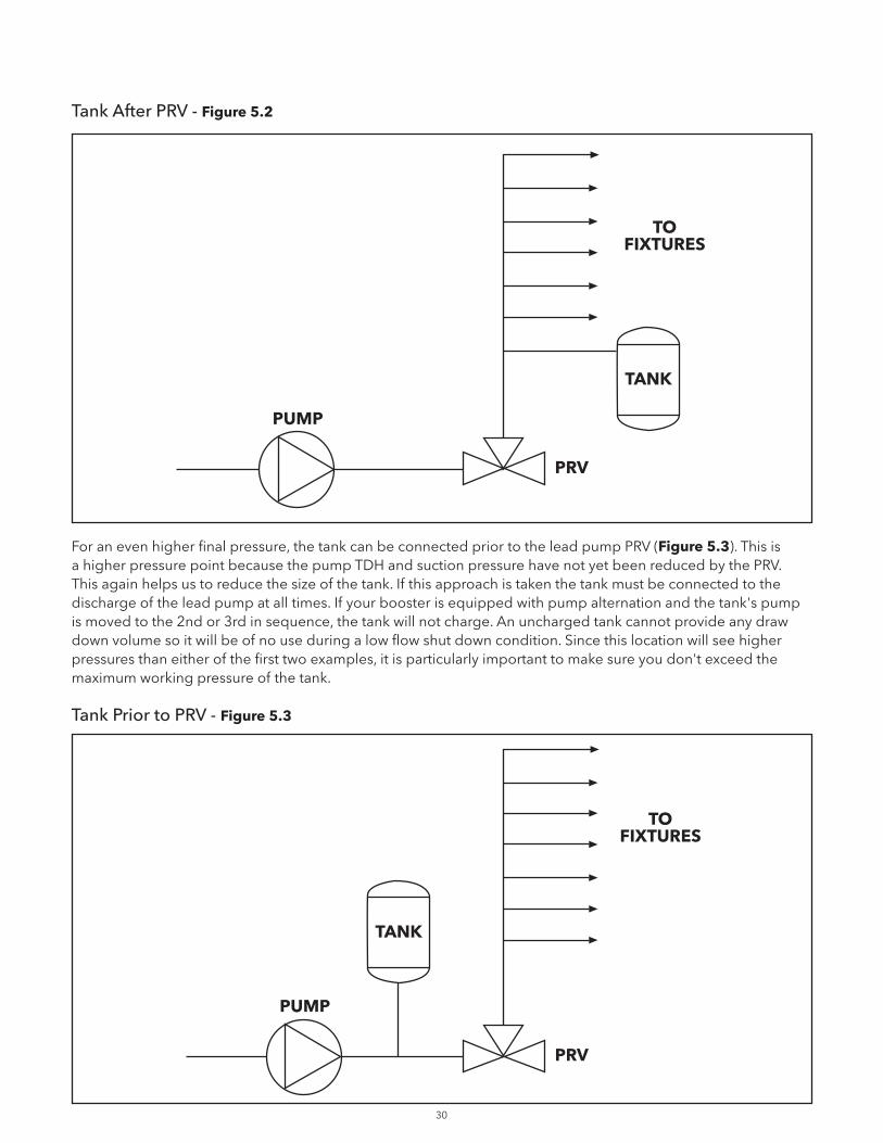
Tank After PRV - Figure 5.2

For an even higher final pressure, the tank can be connected prior to the lead pump PRV (Figure 5.3). This is a higher pressure point because the pump TDH and suction pressure have not yet been reduced by the PRV. This again helps us to reduce the size of the tank. If this approach is taken the tank must be connected to the discharge of the lead pump at all times. If your booster is equipped with pump alternation and the tank's pump is moved to the 2nd or 3rd in sequence, the tank will not charge. An uncharged tank cannot provide any draw down volume so it will be of no use during a low flow shut down condition. Since this location will see higher pressures than either of the first two examples, it is particularly important to make sure you don't exceed the maximum working pressure of the tank.

Tank Prior to PRV - Figure 5.3

PUMP

PRV

TANK

TOFIXTURES

PUMP

PRV

TANK

TOFIXTURES

31

HYDROPNEUMATIC TANK SIZING

First we must determine the tank acceptance volume. Refer to Figure 5.4, below, for a guide to typical acceptance volumes for various facilities. These figures are estimates based on 30 minute shutdown time and should be viewed accordingly.

Figure 5.4

50 8 60 15 15 23 11 15 38

100 15 120 30 30 45 22 30 75

150 23 180 45 45 68 33 45 113

200 30 240 60 60 90 44 60 150

250 38 300 75 75 113 55 75 188

300 45 360 90 90 135 66 90 225

350 53 420 105 105 158 77 105 263

400 60 480 120 120 180 88 120 300

450 68 540 135 135 203 99 135 338

500 75 600 150 150 225 110 150 375

Use this table for estimating purposes only. Final determination of the acceptance volume is the responsibility of the design engineer. Remember to consult local codes!

The thirty minute shut down time can be adjusted for different times by using the following formula:

ACCEPTANCE VOLUME (from Figure 5.4) X DESIRED SHUTDOWN TIME / 30 MINUTES = ADJUSTED ACCEPTANCE VOLUME

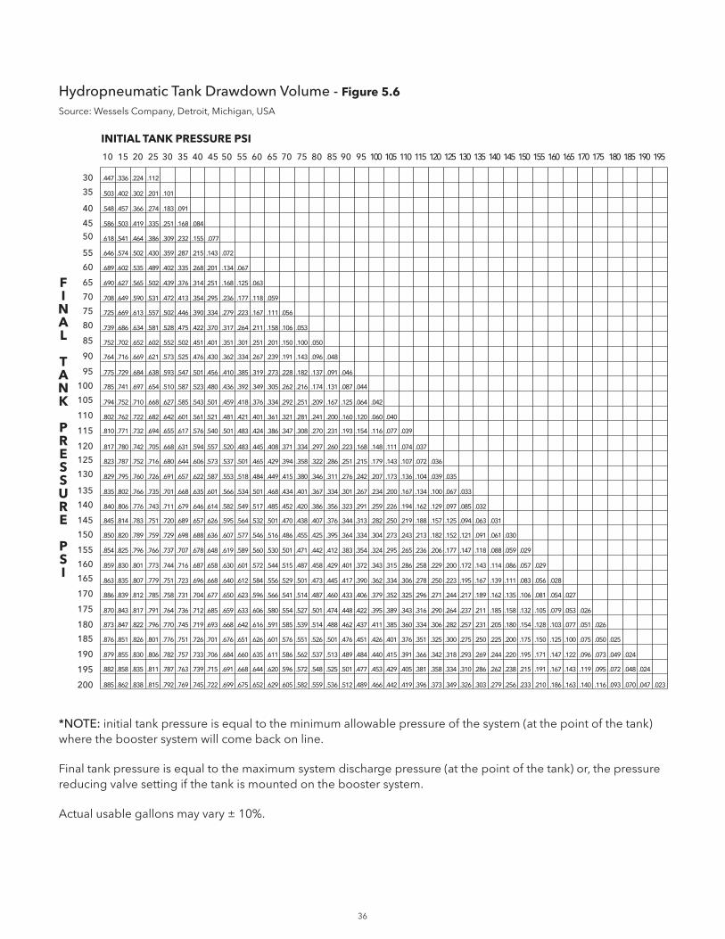
Once we have determined the required acceptance volume, we can calculate the tank size based on draw down capabilities. Consult your hydropneumatic tank supplier for information on draw down volume of their tanks. A typical data sheet is shown in Figure 5.6 on page 36. Since different manufacturer’s tanks have different draw down capabilities, it is imperative that you use the data supplied by the manufacturer whose tank you plan to use.

The value in the intersection of initial pressure and final pressure is your draw down coefficient. Divide your acceptance volume by this coefficient to obtain the total tank volume.

TOTA

L SY

STE

M

DE

MA

ND

(G

PM

)

APA

RTM

EN

T B

UIL

DIN

G

HO

SPIT

AL

SCH

OO

L

UN

IVE

RSI

TY –

C

LASS

RO

OM

S

UN

IVE

RSI

TY –

D

OR

MIT

OR

IES

CO

MM

ER

CIA

L

HO

TEL

PR

ISO

N

32

EXAMPLE #1: TANK ON ROOF

We have a pressure booster sized for 500 GPM at 75 PSIG discharge pressure with a 40 PSIG minimum suction pressure available from the city. The tank will be located on the roof of a 5 story building. Calculate the tank size required for a 15 minute shutdown during low flow conditions and a 65 PSIG booster cut-in pressure:

1. From Figure 5.4, we can see that a booster sized for 500 GPM in an apartment building to be off for 30 minutes on low flow, an acceptance volume of 75 gallons is required. However, since we only need our booster to be off for 15 minutes, we must adjust this acceptance volume accordingly 75 x 15 / 30 = 37.5.

Therefore, our acceptance volume will be 37.5 gallons.

2. Our initial pressure is equal to the pressure at the tank connection point at booster cut in pressure. This value is equal to the cut-in pressure less the static elevation of the tank above the discharge of the booster package. We must also account for the friction loss in the piping between the package discharge and the tank connection point. In this case, we have calculated a friction loss of 10 feet or 4.73 PSIG. The tank is located approximately 70 feet above the booster which equates to 30.3 PSIG.

65 PSIG (CUT IN) - 4.73 PSIG (FRICTION LOSS AT DESIGN FLOW) - 30.3 PSIG (STATIC HEIGHT) = 30 PSIG

3. Final pressure is equal to the pressure at the tank connection point when system is fully pressurized

75 PSIG (SYSTEM PRESSURE) - 4.73 PSIG (FRICTION LOSS AT DESIGN FLOW) - 30.3 PSIG (STATIC HEIGHT) = 40 PSIG

4. Using Figure 5.6, we can determine that our draw down coefficient is .183.

5. Divide the acceptance volume by the draw down coefficient to obtain the total tank volume that will give us 75 GPM during Low flow shutdown.

37.5 GPM / .183 = 205

Therefore, we need a minimum tank volume of 205 gallons to meet our shutdown requirements.

EXAMPLE #2: TANK AT DISCHARGE OF BOOSTER PACKAGE

We again have a pressure booster sized for 500 GPM at 75 PSIG discharge pressure with a 40 PSIG minimum suction pressure available from the city. Now, the tank will be located in the basement of a 5 story building and be connected to the discharge header of the package. Calculate the tank size required for a 15 minute shutdown during low flow conditions and a 65 PSIG booster cut-in pressure:

1. From Figure 5.4, we can see that for a booster sized for 500 GPM in an apartment building to be off for 30 minutes on low flow, an acceptance volume of 75 gallons is required. However, since we only need our booster to be off for 15 minutes, we must adjust this acceptance volume accordingly 75 x 15 / 30 = 37.5.

Therefore, our acceptance volume will be 37.5 gallons.

2. Our initial pressure is equal to cut-in pressure less static height and piping losses to the tank. However, since the tank is located at the discharge of the package, static height and friction losses are insignificant. Therefore, we can conclude that the initial pressure is actually equal to cut-in pressure.

INITIAL PRESSURE = CUT-IN PRESSURE = 65 PSIG.

3. Likewise, the insignificance of static height and friction losses also apply to our calculation of final pressure. We can conclude that final pressure is equal to the pressure at the tank connection point when the system is fully pressurized.

FINAL PRESSURE = SYSTEM PRESSURE = 75 PSIG

33

4. Using Figure 5.6, we can determine that our draw down coefficient is .111.

5. Divide the acceptance volume by the draw down coefficient to obtain the total tank volume that will give us 75 GPM during Low flow shutdown.

37.5 GPM / .111 = 340

Therefore, we need a minimum tank volume of 340 gallons to meet our shutdown requirements.

EXAMPLE #3: TANK CONNECTION BETWEEN PUMP DISCHARGE AND PRV

Using the same pressure booster as the previous two examples, sized for 500 GPM at 75 PSIG discharge pressure with a 40 PSIG minimum suction pressure available from the city. The tank will be located in the basement as in example #2 but will be connected before the pressure reducing valve. Calculate the tank size required for a 15 minute shutdown during low flow conditions and a 65 PSIG booster cut-in pressure:

1. From Figure 5.4, we can see that a booster sized for 500 GPM in an apartment building to be off for 30 minutes on low flow, an acceptance volume of 75 gallons is required. However, since we only need our booster to be off for 15 minutes, we must adjust this acceptance volume accordingly

75 x 15 / 30 = 37.5

Therefore, our acceptance volume will be 37.5 gallons.

2. Our initial pressure is still going to be equal to cut-in pressure as in Example 2. We do not need to be concerned with static height and friction loss since the tank will be located adjacent to the pumps. Therefore, our initial pressure will be equal to cut-in pressure.

INITIAL PRESSURE = CUT-IN PRESSURE = 65 PSIG.

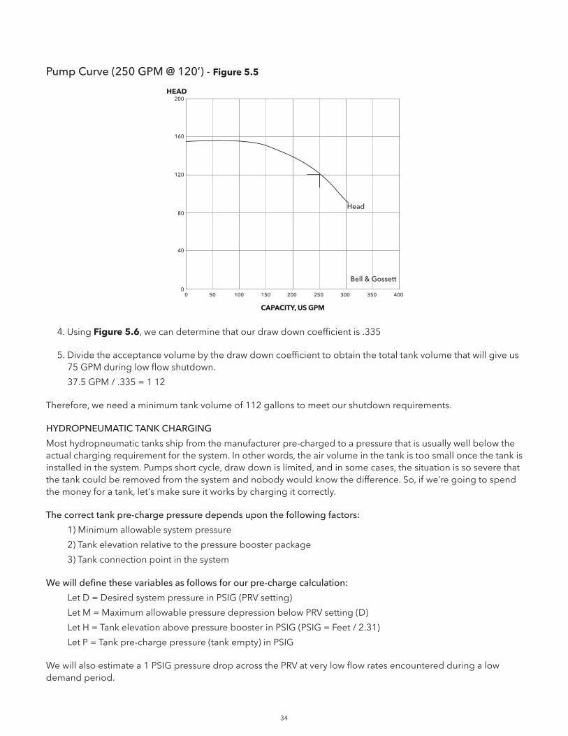
3. Final pressure is going to be significantly higher than in example #2 because our tank is connected to the system prior to the pressure reducing valve. Therefore, we actually have pump TDH at minimal flow plus minimum suction pressure. If our pump has a flow vs. Head curve as shown below in Figure 5.5, the final pressure is going to be 155. (TDH @) 0 GPM) plus minimum suction pressure of 40 PSIG. Therefore, our final pressure can be calculated by adding these values.

67 PSIG (PUMP TDH @ 0 GPM) + 40 PSIG (MIN. SUCTION PRESSURE) = 107 PSIG

34

Pump Curve (250 GPM @ 120’) - Figure 5.5

4. Using Figure 5.6, we can determine that our draw down coefficient is .335

5. Divide the acceptance volume by the draw down coefficient to obtain the total tank volume that will give us 75 GPM during low flow shutdown.

37.5 GPM / .335 = 1 12

Therefore, we need a minimum tank volume of 112 gallons to meet our shutdown requirements.

HYDROPNEUMATIC TANK CHARGING

Most hydropneumatic tanks ship from the manufacturer pre-charged to a pressure that is usually well below the actual charging requirement for the system. In other words, the air volume in the tank is too small once the tank is installed in the system. Pumps short cycle, draw down is limited, and in some cases, the situation is so severe that the tank could be removed from the system and nobody would know the difference. So, if we’re going to spend the money for a tank, let's make sure it works by charging it correctly.

The correct tank pre-charge pressure depends upon the following factors:

1) Minimum allowable system pressure

2) Tank elevation relative to the pressure booster package

3) Tank connection point in the system

We will define these variables as follows for our pre-charge calculation:

Let D = Desired system pressure in PSIG (PRV setting)

Let M = Maximum allowable pressure depression below PRV setting (D)

Let H = Tank elevation above pressure booster in PSIG (PSIG = Feet / 2.31)

Let P = Tank pre-charge pressure (tank empty) in PSIG

We will also estimate a 1 PSIG pressure drop across the PRV at very low flow rates encountered during a low demand period.

0 50 100 150 200 250 300 350 400

CAPACITY, US GPM

HEAD

Head

Bell & Gossett0

40

80

120

160

200

35

If the tank is located above the pressure booster as shown in Figure 5.1 on page 29, the pre-charge is calculated like this:

P = D - M - H - 1

Tanks located approximately level to the booster and connected to the system downstream of the PRV (Figure 5.2, page 30) have their pre-charge pressure as follows:

P = D - M – 1

If the tank is approximately level with the booster but connected to the system prior to the PRV (Figure 5.3, page 30), then we do not have to subtract the 1 PSIG drop across the valve. Therefore, the calculation is as follows:

P = D – M

To confirm the pre-charge pressure of an existing tank, the tank must be isolated from the pumping / piping system. Then the water side of the tank is drained and the air pressure read with a gauge at the air charging valve. This reading is the precharge pressure.

By simply taking a little extra time to make sure our tank is pre-charged correctly, we can be certain that it will serve its purpose of keeping the pumps off during periods of low demand.

PRE-CHARGING EXAMPLE

Let's take a look at the roof tank described in Figure 5.1 on page 29. We know that the correct pre-charge pressure is defined as:

P = D - M - H – 1

We know that:

D = 75

M = system pressure - cut-in pressure = 75 - 65 = 10

H = 70 / 2.31 = 30.3

Therefore, our correct pre-charge pressure is:

75 - 10 - 30.3 - 1 = 33.7 PSIG

To ensure correct operation of the tank during the booster's low-flow shutdown sequence, it must be precharged to 33.7 PSIG.

HYDROPNEUMATIC TANK SUMMARY

As you can see, there are few hard and fast rules to tank sizing. It is predominantly a matter of weighing various factors and compromising on a balance of initial cost and potential energy savings. Locating the tank connection prior to the pressure reducing valve results in the smallest tank but requires its respective pump to always be the lead pump. A tank connection at the discharge header results in a larger tank but allows you to alternate all pumps. A roof mounted tank seems like a pretty reasonable compromise but you must consider the complications of transporting the tank to the roof. In conclusion, tank location has a significant impact on the tank size and must be addressed on a project by project basis.

36

Hydropneumatic Tank Drawdown Volume - Figure 5.6

Source: Wessels Company, Detroit, Michigan, USA

*NOTE: initial tank pressure is equal to the minimum allowable pressure of the system (at the point of the tank) where the booster system will come back on line.

Final tank pressure is equal to the maximum system discharge pressure (at the point of the tank) or, the pressure reducing valve setting if the tank is mounted on the booster system.

Actual usable gallons may vary ± 10%.

INITIAL TANK PRESSURE PSI

FINAL

TANK

PRESSURE

PSI

200

195

190

185

180

175

170

165

160

155

150

145

140

135

130

125

120

115

110

105

100

95

90

85

80

75

70

65

60

55

5045

40

35

30

10 15 20 25 30 35 40 45 50 55 60 65 70 75 80 85 90 95 100 105 110 115 120 125 130 135 140 145 150 155 160 165 170 175 180 185 190 195

.447 .336 .224 .112

.548 .457 .366 .274 .183

.503 .402 .302 .201 .101

.091

.586 .503 .419 .335 .251 .168 .084

.618 .541 .464 .386 .309 .232 .155 .077

.646 .574 .502 .430 .359 .287 .215 .143 .072

.689 .602 .535 .489 .402 .335 .268 .201 .134 .067

.690 .627 .565 .502 .439 .376 .314 .251 .168 .125 .063

.708 .649 .590 .531 .472 .413 .354 .295 .236 .177 .118 .059

.725 .669 .613 .557 .502 .446 .390 .334 .279 .223 .167 .111 .056

.739 .686 .634 .581 .528 .475 .422 .370 .317 .264 .211 .158 .106 .053

.764 .716 .669 .621 .573 .525 .476 .430 .362 .334 .267 .239 .191 .143 .096

.752 .702 .652 .602 .552 .502 .451 .401 .351 .301 .251 .201 .150 .100 .050

.048

.785 .741 .697 .654 .510 .587 .523 .480 .436 .392 .349 .305 .262 .216 .174 .131 .087

.775 .729 .684 .638 .593 .547 .501 .456 .410 .385 .319 .273 .228 .182 .137 .091 .046

.044

.794 .752 .710 .668 .627 .585 .543 .501 .459 .418 .376 .334 .292 .251 .209 .167 .125 .064 .042

.810 .771 .732 .694 .655 .617 .576 .540 .501 .483 .424 .386 .347 .308 .270 .231 .193 .154 .116 .077

.802 .762 .722 .682 .642 .601 .561 .521 .481 .421 .401 .361 .321 .281 .241 .200 .160 .120 .060 .040

.039

.823 .787 .752 .716 .680 .644 .606 .573 .537 .501 .465 .429 .394 .358 .322 .286 .251 .215 .179 .143 .107 .072

.817 .780 .742 .705 .668 .631 .594 .557 .520 .483 .445 .408 .371 .334 .297 .260 .223 .168 .148 .111 .074 .037

.036

.835 .802 .766 .735 .701 .668 .635 .601 .566 .534 .501 .468 .434 .401 .367 .334 .301 .267 .234 .200 .167 .134 .100 .067

.829 .795 .760 .726 .691 .657 .622 .587 .553 .518 .484 .449 .415 .380 .346 .311 .276 .242 .207 .173 .136 .104 .039 .035

.033

.840 .806 .776 .743 .711 .679 .646 .614 .582 .549 .517 .485 .452 .420 .386 .356 .323 .291 .259 .226 .194 .162 .129 .097 .085 .032

.845 .814 .783 .751 .720 .689 .657 .626 .595 .564 .532 .501 .470 .438 .407 .376 .344 .313 .282 .250 .219 .188 .157 .125 .094 .063 .031

.850 .820 .789 .759 .729 .698 .688 .636 .607 .577 .546 .516 .486 .455 .425 .395 .364 .334 .304 .273 .243 .213 .182 .152 .121 .091 .061 .030

.859 .830 .801 .773 .744 .716 .687 .658 .630 .601 .572 .544 .515 .487 .458 .429 .401 .372 .343 .315 .286 .258 .229 .200 .172 .143 .114 .086 .057

.854 .825 .796 .766 .737 .707 .678 .648 .619 .589 .560 .530 .501 .471 .442 .412 .383 .354 .324 .295 .265 .236 .206 .177 .147 .118 .088 .059 .029

.029

.863 .835 .807 .779 .751 .723 .696 .668 .640 .612 .584 .556 .529 .501 .473 .445 .417 .390 .362 .334 .306 .278 .250 .223 .195 .167 .139 .111 .083 .056 .028

.886 .839 .812 .785 .758 .731 .704 .677 .650 .623 .596 .566 .541 .514 .487 .460 .433 .406 .379 .352 .325 .296 .271 .244 .217 .189 .162 .135 .106 .081 .054 .027

.870 .843 .817 .791 .764 .736 .712 .685 .659 .633 .606 .580 .554 .527 .501 .474 .448 .422 .395 .389 .343 .316 .290 .264 .237 .211 .185 .158 .132 .105 .079 .053 .026

.873 .847 .822 .796 .770 .745 .719 .693 .668 .642 .616 .591 .585 .539 .514 .488 .462 .437 .411 .385 .360 .334 .306 .282 .257 .231 .205 .180 .154 .128 .103 .077 .051 .026

.876 .851 .826 .801 .776 .751 .726 .701 .676 .651 .626 .601 .576 .551 .526 .501 .476 .451 .426 .401 .376 .351 .325 .300 .275 .250 .225 .200 .175 .150 .125 .100 .075 .050 .025

.879 .855 .830 .806 .782 .757 .733 .706 .684 .660 .635 .611 .586 .562 .537 .513 .489 .484 .440 .415 .391 .366 .342 .318 .293 .269 .244 .220 .195 .171 .147 .122 .096 .073 .049 .024

.882 .858 .835 .811 .787 .763 .739 .715 .691 .668 .644 .620 .596 .572 .548 .525 .501 .477 .453 .429 .405 .381 .358 .334 .310 .286 .262 .238 .215 .191 .167 .143 .119 .095 .072 .048 .024

.885 .862 .838 .815 .792 .769 .745 .722 .699 .675 .652 .629 .605 .582 .559 .536 .512 .489 .466 .442 .419 .396 .373 .349 .326 .303 .279 .256 .233 .210 .186 .163 .140 .116 .093 .070 .047 .023

37

SECTION 6DOES VARIABLE SPEED PUMPING MAKE CENTS?

The technological advancement in recent years of AC variable frequency drives has brought the marketplace new products that are both more reliable and lower in cost than ever before. We are witnessing much wider use of variable frequency drives on fan and pump applications in the HVAC market because of their ability to greatly reduce annual energy costs. It is not uncommon to see simple paybacks measured in months for HVAC equipment that is being retrofitted with the necessary controls for variable speed operation: pump logic controller, sensors, and variable frequency drives (refer to Figure 6.1). As the cost of electronic equipment continues to decline, more opportunities to apply cost saving variable speed pumping become worthwhile. This technology is now being applied in the plumbing market on domestic water pressure booster systems. Domestic water pressure boosting packages are an attractive application because these systems are significant energy consumers, have widely varying load demands, and are typically oversized.

Domestic water pressure boosting system with adjustable frequency pump drives - Figure 6.1

Maximum Total System Flow — 400 GPM

Required Discharge Pressure — 74 PSIG

30 PSIG Residual Pressure

24 PSIG Static Pressure20 PSIG Friction Head Loss

Minimum Suction Pressure = 20 PSIG

Required Boost = 54 PSIG

NOTE: Two sensors shown for example purposes only. Typically only one sensor is required. See Variable Head Losses (page 39) for details.

WaterHeater

HW CW

Laundry(1st floor)

WaterHeater

HW CW

Kitchen(1st floor)

Administrationand bed tower

LocalPressureSensor

RemotePressureSensor

HW CW

30 PSIG

Pump 1

Pump 2

Pressure Booster System

WaterMeter5 PSIdrop

BackflowPreventer

10 PSIdrop

CityMain

35 PSIGminimum

4-inch pipe

Ad

just

able

freq

uenc

yd

rive

Ad

just

able

freq

uenc

yd

rive

Pum

pco

ntro

ller

38

VARIABLE SPEED PRESSURE BOOSTING

The major argument against using variable speed pumps on a domestic water pressure booster application is that the system curve is relatively flat. Because design discharge pressure must be maintained in the domestic water system regardless of demand, the pump speed range is very limited. Further, since the pump head changes as the square of pump speed, when the pump reduces speed it quickly reduces system pressure. The argument concludes that since the system has little ability to change speed, its ability to save money is reduced, and it is not justifiable. While these general statements are somewhat true, they are not completely accurate. A variable speed pressure booster system can be economically desirable. In fact, this has been proven in the field many times over. However, it is important that each domestic water system be considered individually to determine the desirability for variable speed control. When examining the economic viability of a variable speed pressure boosting system, there are four factors to consider:

1. Pump oversizing

2. Variable head loss

3. Pressure reducing valve (PRV) losses

4. Changing suction pressure

PUMP OVERSIZING

There are few people who would dispute that domestic water booster pump systems are typically oversized. Oversizing begins when the system load is calculated. Loads are usually based on a method of counting the equivalent number of plumbing fixtures and then using a conservative estimate of how many plumbing fixtures will be in operation simultaneously. In addition, the flow for other loads which do not follow normal diversity, such as cooling towers and laundries, are incorporated into the maximum total system flow.

System designers will then customarily use a safety factor to guarantee that the pump is not undersized. An undersized pump will result in a disgruntled customer and possible cost penalties to correct the situation. However, a system with an oversized pump will always work satisfactorily (as long as it is not grossly oversized). In addition, the oversized pump will have the benefit of accommodating future capacity needs.

If the capacity is overstated, the pump head will also be overstated. Since the system pipe size and pressure drop are calculated on an inflated flow rate, the friction losses will be exaggerated. This situation can be compounded when piping head losses are calculated using tables with built-in safety factors.

Another element contributing to oversized pumps is an under-estimated pump suction pressure. The use of a lower than actual suction pressure to calculate boost may be justified due to a lack of suction pressure history, an expected drop in suction pressure because of an aging system, or a municipality that does not keep pace with growth.

All these items added together can result in a significantly oversized pump. The drawback of an oversized pump is wasted energy. The customer pays for the extra capacity with higher operating costs. A pump that is 25% oversized costs approximately 25% more to operate; a 50% oversized pump will cost approximately 50% more to operate. Although overriding can be corrected by trimming the pump's impeller in the field, this practice is rarely done. And if it is, the additional future capacity is lost.

Installing a variable speed system gives you the best of both worlds. A pump with variable speed controls only produces enough head to satisfy the system requirements. The excess capacity is available if it is ever needed, but while in reserve, it is not needlessly consuming energy.

Variable speed systems also allow for system fine tuning. Once a system is installed and operating the required pressure setpoint can be lowered to find the slowest speed at which the system will still satisfy all flow demands. This allows for optimal system performance with minimal effort, and without the additional expense of trimming impellers.

39

VARIABLE HEAD LOSSES

When the total pressure requirement of a system is calculated, the loss due to friction is based on peak demand. However, in actuality, a system seldom reaches a full design load state. During off-peak demand, the system pressure drop is significantly lowered since head loss changes as the square of a change in flow. The term “variable head loss” refers to the changing pressure drop as the draw on the system changes.

The load profile for a domestic water application typically shows the system operating at very low flow rates for long periods of time. In this way, pressure booster systems have an economic advantage over HVAC systems with their classical bell-shaped load profiles. To take full advantage of variable head loss on an open system and save the most energy, the pressure sensor of the variable speed control system must be placed at the most remote or highest point in the system.

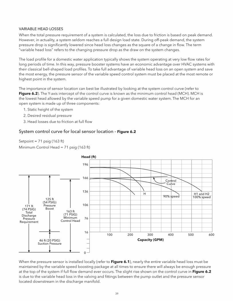
The importance of sensor location can best be illustrated by looking at the system control curve (refer to Figure 6.2). The Y-axis intercept of the control curve is known as the minimum control head (MCH). MCH is the lowest head allowed by the variable speed pump for a given domestic water system. The MCH for an open system is made up of three components:

1. Static height of the system

2. Desired residual pressure

3. Head losses due to friction at full flow

System control curve for local sensor location - Figure 6.2

Setpoint = 71 psig (163 ft)

Minimum Control Head = 71 psig (163 ft)

When the pressure sensor is installed locally (refer to Figure 6.1), nearly the entire variable head loss must be maintained by the variable speed boosting package at all times to ensure there will always be enough pressure at the top of the system if full flow demand ever occurs. The slight rise shown on the control curve in Figure 6.2 is due to the variable head loss in the valving and fittings between the pump outlet and the pressure sensor located downstream in the discharge manifold.

Capacity (GPM)

Head (ft)

ControlCurve

90% speedH H1 and H2

100% speed

100 200 300 400 500 600

0

16

76

106

136

166

196

171 ft(74 PSIG)

TotalDischargePressure

Requirement

125 ft(54 PSIG)Pressure

Boost

46 ft (20 PSIG)Suction Pressure

163 ft(71 PSIG)Minimum

Control Head

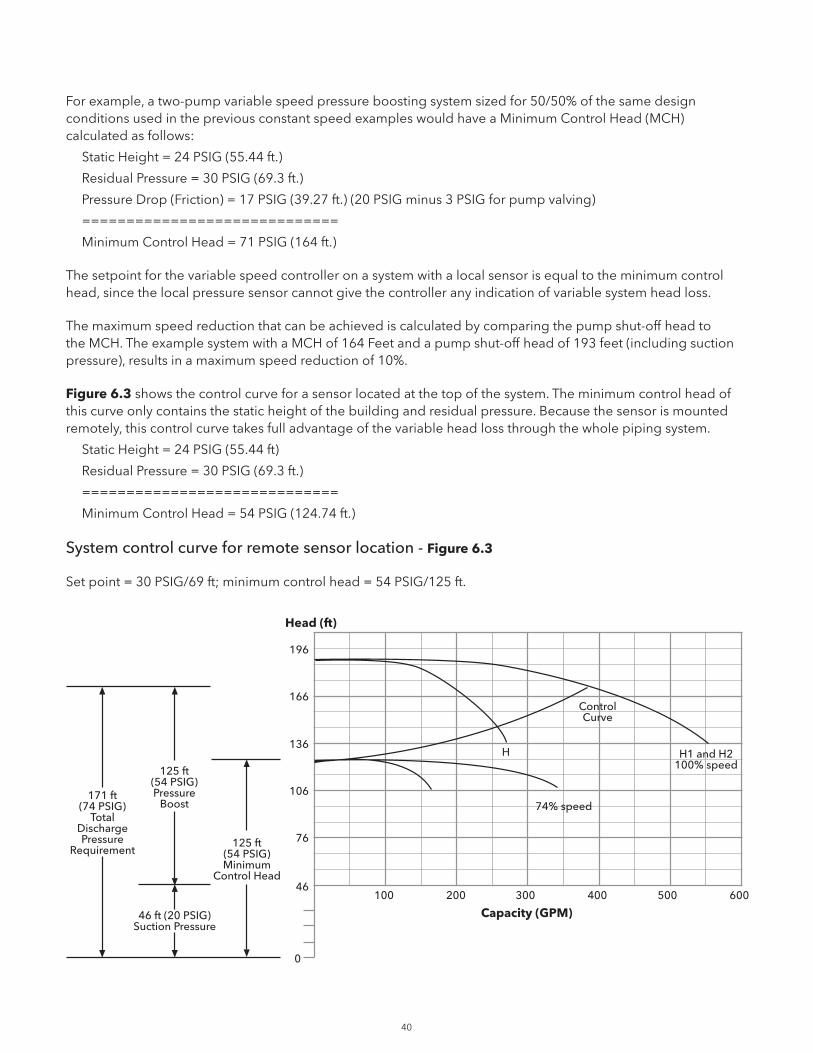
40

For example, a two-pump variable speed pressure boosting system sized for 50/50% of the same design conditions used in the previous constant speed examples would have a Minimum Control Head (MCH) calculated as follows:

Static Height = 24 PSIG (55.44 ft.)

Residual Pressure = 30 PSIG (69.3 ft.)

Pressure Drop (Friction) = 17 PSIG (39.27 ft.) (20 PSIG minus 3 PSIG for pump valving)

=============================

Minimum Control Head = 71 PSIG (164 ft.)

The setpoint for the variable speed controller on a system with a local sensor is equal to the minimum control head, since the local pressure sensor cannot give the controller any indication of variable system head loss.

The maximum speed reduction that can be achieved is calculated by comparing the pump shut-off head to the MCH. The example system with a MCH of 164 Feet and a pump shut-off head of 193 feet (including suction pressure), results in a maximum speed reduction of 10%.

Figure 6.3 shows the control curve for a sensor located at the top of the system. The minimum control head of this curve only contains the static height of the building and residual pressure. Because the sensor is mounted remotely, this control curve takes full advantage of the variable head loss through the whole piping system.

Static Height = 24 PSIG (55.44 ft)

Residual Pressure = 30 PSIG (69.3 ft.)

=============================

Minimum Control Head = 54 PSIG (124.74 ft.)

System control curve for remote sensor location - Figure 6.3

Set point = 30 PSIG/69 ft; minimum control head = 54 PSIG/125 ft.

Capacity (GPM)

Head (ft)

ControlCurve

74% speed

H H1 and H2100% speed

100 200 300 400 500 600

0

46

76

106

136

166

196

171 ft(74 PSIG)

TotalDischargePressure

Requirement

125 ft(54 PSIG)Pressure

Boost

46 ft (20 PSIG)Suction Pressure

125 ft(54 PSIG)Minimum

Control Head

41

Since a remotely mounted pressure sensor is reading the pressure at the point of use, the variable speed controller setpoint for the remote sensor is equal to the desired pressure at that point. In our example, the desired residual pressure is 30 PSIG. The maximum speed reduction in our example system with a remotely mounted sensor improves to 26%.

A variable speed control system with a remote sensor has the ability to follow a steeper control curve allowing slower operating speeds and increased cost savings. Since pump horsepower changes as the cube of the speed, even small changes in speed can have a significant effect on operating costs. Remember domestic water systems operate mostly at reduced flow demand conditions.

The following table summarizes the effects of sensor location on our example system:

LOCAL SENSOR REMOTE SENSOR

Setpoint 71 PSIG 30 PSIG

Minimum Control Head 164 Feet 125 Feet

Control Curve Little change with flow Significant head reduction

at lower flows

Speed reduction achievable 10% 26%

(assuming constant suction pressure)

It becomes obvious, looking at the control curves, that a piping system that has a higher ratio of variable head losses to fixed head elements will be a better candidate for variable speed controls than a system with a lower ratio.

The type of building and application play an important role in determining the shape of the control curve and load profile of the system. A tall residential apartment building with its large static height requirement will have a very different fixed head/variable head ratio than a large sprawling one-story factory.

PRESSURE REDUCING VALVE LOSSES

A pressure reducing valve (PRV) is used on constant speed domestic water pressure booster systems as a means of pressure control by modulating open and closed to maintain a constant discharge pressure. Some of the benefits of the PRV are that it:

1. Maintains steady system pressure regardless of changes in demand or suction pressure.

2. Helps prevent system over-pressurization.

3. Allows the use of dissimilar pumps in parallel by preventing a higher head pump from closing the check valve of a pump with lower head.

These major benefits can be summarized by the fact that the PRV absorbs the pump's excess energy. The drawback to the PRV is that the absorbed energy is wasted energy. Variable speed systems achieve proper pressure by changing the pump's speed and therefore do not waste the excess energy. Figure 6.4 examines the operating point of our example system at a reduced flow rate. On a constant speed system, variable flow is achieved by riding back and forth on the pump curve. At lower flow rates, the PRV chokes down to absorb the excess head produced by the pump as its head rises to shut-off.

42

System control curve for remote sensor location at reduced flow rate - Figure 6.4

Set point = 30 PSIG/69 ft; minimum control head = 54 PSIG/125 ft.

Variable speed systems, however, track the control curve. Lower head and flow rates are the result of slowing down the pump. The energy saved by a variable speed pump for this one flow rate is calculated below:

Constant Speed Brake Horsepower = (Flow * GPM ) / (3960 * Pump Eff)

= (100 * 143) / (3960 * .72) = 5.0 BHP

Constant Speed kW = (BHP / Motor Eff / 1.34

= (5.0 HP / .852) / 1.34 = 4.4 kW

Variable Speed Brake Horsepower = (100 * 81.7 / 3960 * .57 = 3.6 BHP

Variable Speed kW = (BHP / Motor & Drive Eff / 1 .34

= (3.6 HP / .83) / 1.34 = 3.2 kW

Net Energy Savings = (4.4 - 3.2) = 1.2 kW (approximately 27%)

As stated above, one of the reasons for utilizing pressure reducing valves on each constant speed pump is to protect against over-pressurizing the domestic water booster system. If a constant speed pump without a PRV on its discharge is turned on when there is little flow demand in the system and the actual suction pressure is much greater than design, the resulting pressure from that pump could possibly over-pressurize the system and create leaks and/or damage plumbing fixtures. This same scenario could occur on a variable speed control system that is supplied with an across-the-line VFD bypass. If an across-the-line VFD bypass is desired because of the critical nature of the domestic water system and greater redundancy is required, then each pump with this capability should also be supplied with a pressure reducing valve on its discharge or some other means of pressure control. This will protect the domestic water system against over-pressurization in the event the pump is needed to run through the constant speed VFD bypass.

Capacity (GPM)

Pump TotalDeveloped

Head and Suction Pressure (ft)

ControlCurve

74% speed

H H1 and H2100% speed

100 200 300 400 500 600

0

46

76

106

136

166

196

171 ft(74 PSIG)

TotalDischargePressure

Requirement

125 ft(54 PSIG)Pressure

Boost

46 ft (20 PSIG)Suction Pressure

125 ft(54 PSIG)Minimum

Control Head

Pump TotalDeveloped

Head (ft)

Constant Speed Operating Point

Variable SpeedOperating Point

0

20

40

60

80

100

120

140

160

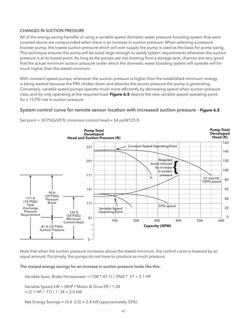
43

CHANGES IN SUCTION PRESSURE

All of the energy saving benefits of using a variable speed domestic water pressure boosting system that were covered above are compounded when there is an increase in suction pressure. When selecting a pressure booster pump, the lowest suction pressure which will ever supply the pump is used as the basis for pump sizing. This technique ensures the pump will be sized large enough to satisfy system requirements whenever the suction pressure is at its lowest point. As long as the pumps are not drawing from a storage tank, chances are very good that the actual minimum suction pressure under which the domestic water boosting system will operate will be much higher than the stated minimum.

With constant speed pumps, whenever the suction pressure is higher than the established minimum, energy is being wasted because the PRV chokes down and absorbs the excess pressure the pump is generating. Conversely, variable speed pumps operate much more efficiently by decreasing speed when suction pressure rises, and by only operating at the required load. Figure 6.5 depicts the new variable speed operating point for a 15 PSI rise in suction pressure.

System control curve for remote sensor location with increased suction pressure - Figure 6.5

Set point = 30 PSIG/69 ft; minimum control head = 54 psiW125 ft.

Note that when the suction pressure increases above the stated minimum, the control curve is lowered by an equal amount. Put simply, the pumps do not have to produce as much pressure.

The revised energy savings for an increase in suction pressure looks like this:

Variable Span, Brake Horsepower = (100 * 47.1) / 3960 * .57 = 2.1 HP

Variable Speed kW = (BHP / Motor & Drive Eff / 1.34= (2.1 HP / .77) / 1 .34 = 2.0 kW

Net Energy Savings = (4.4 -2.0) = 2.4 kW (approximately 55%)

Capacity (GPM)

Pump TotalDeveloped

Head and Suction Pressure (ft)

Required boost reduced

by increasein suctionpressure

59% speed

H H1 and H2100% speed

100 200 300 400 500 600

0

81

111

141

171

201

231

171 ft(74 PSIG)

TotalDischargePressure

Requirement

90 ft(39 PSIG)Pressure

Boost

81 ft (35 PSIG)Suction Pressure

125 ft(54 PSIG)Minimum

Control Head

Pump TotalDeveloped

Head (ft)

Constant Speed Operating Point

Variable SpeedOperating Point

0

20

40

60

80

100

120

140

160

{

44

Putting it all together...

An economic analysis comparing a constant speed domestic water pressure boosting system to a variable speed control system can be done quickly through the use of sophisticated software packages that model the system. Our sample system discussed on page 37 was modeled using $0.10 / kWH and the following suction pressure profile:

Suction Pressure % of Year

20 PSIG 33%

25 PSIG 33%

35 PSIG 34%

The results are shown in the table below:

SYSTEM ANNUAL OPERATING COST

Two constant speed pumps $6,792 Two variable speed pumps Local Sensor $3,56650/50% pump split 50/50% pump split

Three constant speed pumps $6,779 Two variable speed pumps Remote Sensor $2,537

33/33/33% pump split 50/50% pump split

Retrofitting Variable Speed controls to a Constant Speed Booster

Converting a constant speed pressure booster to variable speed operation is a fairly straightforward task. There are a few factors that need to be addressed. If your system consists of identical pumps without pressure reducing valves, the conversion is quite simple. Simply remove the existing starter panel and install the variable frequency drives, controller and remote sensor. Remember the advantages of a remote sensor discussed a few pages ago.

If you have pressure reducing valves on your system, they must either be removed, modified or set above the normal required discharge of the pump at design conditions. The purpose of a PRV on a constant speed system is to limit the discharge pressure of the pump when a suction pressure surge occurs or when the pump rides back on its curve. This action will cause the PRV to “fight” the variable speed controller. Since the PRV regulates the discharge pressure, it is difficult for the system to exceed set point. If we do not exceed the set point, the controller sees no reason to slow the AFD down or destage pumps. Therefore, if the PRV situation is not properly addressed, variable speed operation becomes a defacto constant speed system.

Fortunately, it is relatively simple to avoid the PRV dilemma. The most straightforward option is to replace the PRV with a check valve. If this is not feasible, the PRVs pilot valve can be removed. This essentially converts the PRV to a check valve only. The drawback to this shortcut is that the PRV is going to have a greater pressure drop than a typical check valve of the same size. This additional pressure drop can be significant and causes our system to use additional horsepower to overcome the pressure drop. The decision to replace or modify the PRV must be approached on a case by case basis. Weigh the cost of replacing the valve against the additional energy cost that will be incurred by pumping through the modified PRV.

Variable Speed Systems With Pressure Reducing Valves

There is a situation where it is advisable to use PRVs in variable speed applications. If you plan to have a VFD bypass on your system, consider a means to avoid over-pressurizing the system when operating in bypass. Remember, in the bypass mode, the pump is running at full speed regardless of the process variable vs. set-point relationship. Set point is defined as the pressure we want to maintain at the sensor location and process variable is what the pressure actually is at that point. The controller's primary function is to control pump speed and staging sequence to keep process variable equal to set-point. If the dead head pressure of the pump plus maximum suction pressure is sufficient to generate a system pressure high enough to damage any fixtures, you need a pressure reducing valve.

45

This seems to contradict everything we just stated, but it doesn't necessarily do so. If we set the PRVs for a pressure higher than what the pump needs to generate at the design point but low enough to prevent fixture damage the PRV will simply act as a check valve. The reducing action of a PRV really does not come into play until we get very close to the valve's set point. If we can set it high enough (10 PSIG typical) above the normal pump discharge pressure at design point the valve will not fight the variable speed operation. When the system is in bypass it could generate enough pressure to activate the reducing function of the valve.

Because of the substantial pressure drop across most PRVs, it is best to avoid them in variable speed pressure boosters. However, in applications where it is not feasible or not desirable to eliminate them, they can be effectively integrated into the system.

Multi-pump Variable Speed Boosters With Jockey Pumps

As a general rule, it is unnecessary to use a jockey pump with a multi pump variable speed pressure booster. A jockey pump is a small lead pump utilized to satisfy demand during low flow conditions. The intent is to save energy by running a low horsepower pump instead of one of the higher horsepower Iag pumps. On a constant speed system, this makes perfect sense. In a variable speed system, the energy savings associated with a jockey pump is most likely insignificant.

If your variable speed control system is designed properly, during low demand conditions, one pump will be operating at a speed just high enough to keep the setpoint satisfied. If we look at the energy consumption of this pump vs. the energy consumption of a small jockey pump, there will most likely be very little difference. If you weigh the cost of the jockey pump including valving and installation against the operating cost difference, you will most likely find the jockey pump to be expendable.

On very large systems, it may be cost effective to use a jockey pump. The main pump horsepower would have to be great enough to cause that motor to consume significantly more energy at low speed than a constant speed jockey pump. The control sequence in this case would start the jockey pump upon a detection of demand on the system. The jockey pump would operate alone up to a given flow rate. When this flow rate is reached, the main pump(s) are started and the jockey pump is destaged. Upon a decrease in demand, the jockey pump is re-started and the main pumps are again shut down. It is critical to include the appropriate proof timers to adequately fine tune the system and avoid pump short-cycling.

If a constant speed jockey pump is used, it is necessary to install a pressure reducing valve on the pump discharge. Since we are not varying the speed of this pump, the PRV is required to maintain a constant discharge pressure to protect the system from over-pressurization.

HYDROPNEUMATIC TANKS

A surprising number of people are under the impression that hydropneumatic tanks are not required with a variable speed pressure booster. While it is true that the variable speed system will function without the tank, so will a constant speed booster. As in the case of a constant speed booster the tank on a variable speed system is used to satisfy small demands while the unit is in no-flow shutdown mode. Without the tank, the pumps cannot be effectively shut down during periods of very low demand. Since the primary goal of variable speed pumping is energy savings, it makes sense to save more by utilizing the no-flow shutdown circuitry. Furthermore, since the tank acts as a “shock absorber” the variable speed system will be less prone to abrupt variations in speed.

46

SUMMARY

Applying variable speed controls to a domestic water pressure booster system can be a financially attractive opportunity with today's advanced variable speed pump control systems. The control system is extremely important when it comes to variable speed domestic water pressure boosting because the response of the system is far quicker than the typical HVAC system. Flow demands in a domestic water system vary greatly over short periods of time, and as such, the control system must be capable of tracking those fast changing loads. The situation is even more critical when staging and destaging multiple variable speed pumps in parallel. If the pump controller response is too greatly dampened, the demand requirement for an additional pump may come and go before the Iag pump ever gets started. If the decision is made to provide a variable speed domestic water pressure booster system with across-the-line VFD bypass capabilities, be certain the piping system is protected against over-pressurization. Keep in mind that for systems with across-the-line VFD bypass equipment and no means of pressure control, the risk of over-pressurizing the system is greater with higher-than-minimum design suction pressures. Nonetheless, significant energy savings over traditional constant speed systems will be realized if applied and controlled properly. Therefore, each domestic water pressure booster system should be analyzed individually, taking into account local and remote pressure sensor locations and varying suction pressures.

47

Xylem Inc. 8200 N. Austin Avenue Morton Grove, Illinois 60053 Phone: (847) 966-3700 Fax: (847) 965-8379www.bellgossett.com

Bell & Gossett is a trademark of Xylem Inc. or one of its subsidiaries. © 2018 Xylem Inc. TEH-1096B February 2018

1) The tissue in plants that brings water upward from the roots;2) a leading global water technology company.

We’re a global team unified in a common purpose: creating advanced technology solutions to the world’s water challenges. Developing new technologies that will improve the way water is used, conserved, and re-used in the future is central to our work. Our products and services move, treat, analyze, monitor and return water to the environment, in public utility, industrial, residential and commercial building services, and agricultural settings. With its October 2016 acquisition of Sensus, Xylem added smart metering, network technologies and advanced data analytics for water, gas and electric utilities to its portfolio of solutions. In more than 150 countries, we have strong, long-standing relationships with customers who know us for our powerful combination of leading product brands and applications expertise with a strong focus on developing comprehensive, sustainable solutions.

For more information on how Xylem can help you, go to www.xyleminc.com

Xylem