Domestic Trade Frictions and Agriculture

Sebastian Sotelo

University of Michigan∗

This version: June 16, 2016

First version: May 9, 2015

Abstract

I develop a model of heterogeneous land quality and study the relation between

trade, farming productivity and welfare in Peru, where high domestic and interna-

tional trade costs pose a major barrier to efficient farming. To quantify the model, I

use a new dataset on spatially disaggregated crop prices, yields and land allocations.

I then use the model to measure the welfare and productivity effects of two shocks to

trade opportunities. First, I study a policy of paving roads, which raises average pro-

ductivity and welfare (16% and 4%), but causes some regions to lose due to increased

competition from remote suppliers. Second, I study a shock to international prices

that spreads unevenly across regions, generates heterogeneous price adjustments and,

therefore, has distributional consequences that differ from those of a standard small

open economy model.

Keywords: assignment models, trade costs, equilibrium, agriculture, productivity

JEL Codes: F11, O13, Q17, D58

∗I am indebted to Sam Kortum, Nancy Stokey, and Thomas Chaney for their advice and encouragement. I also thank

Fernando Alvarez, Costas Arkolakis, David Atkin, Saki Bigio, Lorenzo Caliendo, Kerem Cosar, Javier Cravino, Alan Deardorff,

Jonathan Eaton, Jeremy Fox, Sara Heller, Erik Hurst, Gita Khun Jush, Andrei Levchenko, Joaquin Lopez, Sara Moreira,

Ralph Ossa, Edgar Salgado, Danny Tannenbaum, Adriaan Ten Kate, and Mike Waugh, as well as participants in seminars

at UChicago, Yale, the Minneapolis Fed, the St. Louis Fed, Michigan, Penn State, the Fed Board, Drexel, Toronto, Brown,

DePaul, the Philadelphia Fed for helpful comments and suggestions at different stages of this project. Special thanks to Alan

Sanchez and Ben Faber for detailed discussions. Maria Alejandra Zegarra provided excellent research assistance. Part of this

paper was written while I was visiting the Economics Department at Yale University. Funding from the Sjaastad Research

Fellowship Fund is gratefully acknowledged. Finally, I would like to thank Ministerio de Transportes y Comunicaciones de Peru

and Ministerio de Agricultura y Riego de Peru for sharing their data with me. All opinions and remaining errors are my own.

This paper circulated previously as “Trade Frictions and Agricultural Productivity: Theory and Evidence from Peru.” E-mail:

ssotelo@umich.edu

1

1 Introduction

In developing countries, a large majority of the poor live in rural areas. Their livelihoods

are often tied to unproductive agriculture, limited by major barriers to trade such as poor

infrastructure, adverse geography, and the spatial dispersion that is characteristic of rural

populations. Not surprisingly, researchers and policy makers perceive the costs of domestic

and international trade as a drag on incomes and productivity.1

Assessing the welfare and productivity effects of shocks to trade opportunities (such as

infrastructure policy), requires an understanding of how individual farmers and consumers

react to these shocks, and how their choices interact in the aggregate. On the one hand,

policies that reduce trade costs can increase allocative efficiency and welfare by unlocking

the forces of comparative advantage and the use of modern inputs. On the other hand,

such policies also affect the equilibrium prices of crops, especially of those that are traded

only domestically. Because these crops usually constitute an important part of the diet of

subsistence farmers and net food buyers, improved exchange opportunities also affect welfare

through their effect on consumption prices.

In this paper, I develop a framework to measure the consequences of trade-related shocks

to the agricultural sector, and quantify it using Peruvian data. I start by documenting four

facts about agriculture in Peru that guide my modeling choices. First, there is substantial

price dispersion across regions, indicative of domestic trade costs. Moreover, prices are higher

in urban areas and the prices of export crops rise with proximity to ports, consistent with

the presence of domestic and international trade. Second, farmers within a region allocate

land to many crops and, third, average revenue per unit of land varies substantially across

crops. These two facts suggest that land quality varies within regions and that crops require

land with different intensities. Fourth, the quality of roads varies throughout the country,

which produces variation in trade costs.

Informed by these facts, I then develop a quantitative model of specialization and trade.

In the model, farmers can grow various crops on land plots of varying quality. They can

also trade their crops, at a cost, for intermediate inputs, non-agricultural goods, and other

crops, in local, urban, and international markets. Differences in land quality across regions

and in land intensity across crops generate domestic and international trade, while domestic

trade costs discourage it. The resulting model is a hybrid between a small open economy

1According to the World Bank’s World Development Report, as of 2002, 75% of the world poor were ruraldwellers (The World Bank (2007)). The same Report relates developing countries’ agricultural performanceto within-country variation in access to markets and land quality (p. 54). Likewise, a recent Inter-AmericanDevelopment Bank report reflects on how transport costs limit overall exporting activity: “high domestictransport costs can push exports to concentrate in just a few areas [...], while squeezing gains or simplylocking out of trade large swaths of the country” (Mesquita Moreira, Blyde, Volpe, and Molina (2013), p. 3.)

2

(SOE), which takes international prices as given, and a closed economy, where prices are

determined by regional trade within the country. The equilibrium features price dispersion

and incomplete land specialization across regions, as in the data. Moreover, productivity

and welfare are determined by market access and comparative advantage.

To quantify the theory, I construct a novel data set combining several sources of data on

Peruvian agriculture. I use government statistics on land allocation, production, and prices

to estimate crop-specific land quality across and within regions. To estimate within-country

trade frictions, I bring in a complete dataset of the transportation system of Peru. Finally,

I use disaggregated household consumption data to estimate the elasticity of substitution

across crops.

Once I have quantified the model, I conduct two counterfactual experiments that illus-

trate how improved exchange opportunities affect welfare and productivity in the context

of imperfect regional integration. I first simulate an infrastructure policy of paving major

existing roads in Peru, which reduces domestic trade costs. Second, I simulate a shock to

international crop prices. In both counterfactual scenarios, the key to understanding pro-

ductivity and welfare effects are: (i) the initial production and consumption allocations,

driven by comparative advantage, and (ii) the endogenous adjustment of prices in each re-

gional market, which depend also on the substitutability of crops in production -linked to

the degree of land heterogeneity– and in consumption.

To understand how improved roads affect farming productivity, note that, when access

to markets is costly, farmers pay high prices for their purchases and collect low prices for

their sales. Consequently, they specialize less according to comparative advantage and also

cut back their use of intermediate inputs. In this setting, a simulated, country-wide policy

that paves existing major roads increases a multi-crop index of TFP in agriculture in almost

every region (16% on average).

The welfare effects of this policy are more subtle, since it also tends to reduce the price of

crops relative to the rest of the economy. While the policy increases the price a farmer fetches

for his products by improving his own access to domestic and international markets, the

policy also improves the access of farmers in other regions, increases the supply of the same

crops to domestic markets and thus decreases their price. On average, farmers experience 4%

welfare gains. But a farmer in the 25th percentile of the distribution of welfare changes loses

5%, while one in the 75th gains 12%. Rural dwellers employed in the non-agricultural sector

mostly benefit as a result of the policy, but can lose in remote areas where consumption

prices increase.

In the second counterfactual exercise, I simulate a shock to international crop prices.

In line with a World Bank scenario for the Doha trade talks, this exogenous shock mildly

3

increases the international price of cereals and cotton, relative to other crops. While net

sellers of those crops tend to gain and net buyers tend to lose, unlike in a small open

economy, international shocks spread unevenly in regional markets. Proximity to ports

increases the transmission of international shocks not only to internationally traded crops

but, importantly, to non-traded crops. Even for a small shock, these general equilibrium

effects can be quantitatively important, leading to the opposite welfare prediction of a simple

SOE model in about 27% of regions.

In addition to producing substantive results for Peru, this paper also makes three method-

ological contributions. First, the theory connects tightly with data on land allocations and

productivity, enabling the estimation of the model based solely on agricultural and aggregate

trade statistics, which are collected by many countries. This approach is especially useful for

studying economies where trade also occurs within borders, because it sidesteps the need to

use domestic trade data, often a limiting factor.

Second, the model treats crops as homogeneous goods. This choice allows for a simple

analysis of the dissemination of price shocks across regional markets, based only on initial

consumption and land shares and the elasticities of supply and demand. Moreover, when

studying trade within a country, this treatment provides a useful alternative to the stan-

dard assumption that goods are regionally differentiated (Armington) which, besides being

implausible at high spatial resolutions, forces all regions to trade bilaterally in all goods. In

contrast, the model in this paper generates sparse trade patterns – a well-known feature of

trade data – without resorting to infinite trade costs. As I show, finding the equilibrium in

this model requires solving a system of equations with complementarity constraints, where

the latter link, for each crop, the price difference and the trade flow between each pair of

regions. This is a challenging, but well-understood numerical problem.

Third, I obtain a simple estimating equation for the elasticity of land allocation with

respect to relative prices, a key quantity governing adjustments to shocks. The estimating

equation captures a basic economic intuition inherent to models where factors of production

are heterogeneous: As more land is allocated to a crop, the average productivity of the land

used to grow that crop decreases, with an elasticity directly related to the heterogeneity of

land. This parameter also governs all cross-elasticies in production – a practical compro-

mise when the availability of few cross sections of land use and prices limits the number of

parameters that can be estimated.

Peru is an ideal setting for this study because its geography is diverse, and its agriculture

shares features with developed and developing countries alike. It is a middle income country

where a few large urban markets are often the destination of traded agricultural produce,

but where some well-connected regions produce for export markets. Eighty six percent

4

of the national highway system is unpaved, yet dirt roads coexist with modern highways.

Geography also plays a major role in shaping trade patterns: the country is divided in

two by the Andes, with rainforests to the east and deserts and fertile valleys to the west.

Transport and geography in Peru produce large variation in access to markets, as shipping

crops even between relatively close locations can be very costly.2 Geography is also a basis

for specialization based on comparative advantage, because weather and land quality vary

drastically within the country. And while large farms on the coast often employ modern

techniques, isolated Andean and jungle regions still use traditional farming methods. Finally,

about 25 percent of the labor force is employed in agriculture, much like in other developing

countries.3

This paper relates to the literature on equilibrium models of trade in agriculture, such

as Costinot, Donaldson, and Smith (2016), Fajgelbaum and Redding (2014), Costinot and

Donaldson (2014) and Costinot and Donaldson (2012), who study how trade opportunities

mitigate climate change, drive structural transformation, and improve welfare. I make several

contributions to this literature. I provide a parsimonious framework to study prices and

allocations when regions that produce homogeneous goods are partially integrated with each

other and the rest of the world. These modeling elements are important in my application

to Peru and can provide an apt description of other developing economies. Yet, in terms

of the general equilibrium structure of the model, they entail a strong departure from the

literature and provide new insights on the regional adjustment to trade shocks. The model

allows me to trace separately the effect of domestic trade costs on productivity through

specialization and input use. I also show how to incorporate different land-use intensities

across crops into a tractable model of production. Finally, unlike Donaldson (2015), who

integrates the Ricardian model of Eaton and Kortum (2002) with Indian regional trade data,

my model yields predictions for land shares across crops; this allows me to make contact with

land use data, which is more widely available than data on within-country trade. In this

context, I measure land heterogeneity using an equilibrium relationship between data on

land allocations and measures of potential yields from standard agronomic models.4

More broadly, this paper also speaks to the literature that documents the role of agri-

culture in the low productivity of developing countries (Gollin, Lagakos, and Waugh (2013)

and Restuccia, Yang, and Zhu (2008)) and proposes explanations for this finding, such as

2For example, in 2013 a 209 kilometer (130 mile) trip from the district of Uchumarca to the district ofChachapoyas doubles the price of a kilogram of potatoes due to freight rates alone (source Regional Directionof Agriculture, La Libertad).

3The share of labor in agriculture in developing countries ranges from 64 percent in Sub-Saharan Africato 22 percent in Eastern Europe and Latin America (See World Bank, 2008, p.27-28).

4These are the data in the Global Agro-Ecological Zones (IIASA/FAO (2012)) also used in Costinot andDonaldson (2014) and Costinot and Donaldson (2012).

5

worker sorting across sectors (Lagakos and Waugh (2013)), policy barriers to efficient farm

size (Adamopoulos and Restuccia (2014)), and trade frictions (Tombe (2015), Adamopoulos

(2011), and Gollin and Rogerson (2014)). This paper shows that transportation technology

in developing countries is a constraint that limits the use of modern inputs, and that improv-

ing this technology can lead to a more productive allocation of land and labor. To do so,

it develops a quantitative model of spatial equilibrium that focuses on domestic trade costs

and, after estimating them directly, measures their impact on factor allocation, productivity,

and incomes.

2 Four motivating facts

In this section, I document four observations about agriculture in Peru and explain how those

facts motivate my modeling approach. First, there are large, systematic differences in crop

prices across regions, and between urban and rural areas, indicative of domestic barriers to

trade. Second, regions tend to grow many crops, which suggests land quality heterogeneity.

Third, average revenue per unit of land varies significantly across crops, which suggests

that crops use land with different intensities. Fourth, road quality varies throughout the

country. The sample I use throughout contains the top 20 crops by value of production, in

194 provinces in Peru.5

There are large spatial differences in farm gate and consumer prices. Figures 1(a)

and 1(b) give an example of variation in farmgate prices across regions using coffee, one of

Peru’s main exports. The left panel displays the large variation in the price of coffee across

regions that produce it, while the second shows that farmgate prices decline with distance

to the capital (Lima), which also contains the main sea port.

To test whether prices are systematically different across regions, we can use unit values

calculated from household surveys, which approximate consumer prices and for which we

have many observations per region (Deaton (1997), Ch. 7). Table 1 shows the results of

regressing log unit values on two different sets of dummies. Column 1 shows, for each crop,

the F statistic of a joint significance test for region dummies. Indicative of spatial dispersion,

we reject the null that these dummies have no explanatory power. Column 2 shows the R2 of

5I obtain the first three observations using a national data set on agricultural statistics and householdconsumption surveys. The crops included in the analysis are rice, potato, coffee, yellow maize, alfalfa,asparagus, banana, cassava, amilaceo maize, grape, cotton, onion, choclo maize, bean, avocado, wheat,cacao, orange, barley, and tangerine. To obtain the fourth observation I use a comprehensive dataset on theroad system in Peru. The details of the construction of the data set are contained in Section 5 and AppendixJ.

6

the regression, which indicates that a large fraction of the price variation is spatial. Columns

3 and 4 report the coefficient and standard error of regressing log unit values on a dummy

for whether the observation corresponds to an urban area. These regressions show that

consumer prices in urban areas are usually higher than in rural areas, ranging from -0.02 to

0.6 log points higher.6

These spatial price differences suggest that trade barriers prevent price equalization, and

are consistent with urban centers importing food from rural areas. They illustrate that for

some crops, such as coffee, international markets exert an effect on domestic prices. Hence,

in what follows I write down a model that includes domestic trade frictions, that allows

for international and domestic trade, and where a non-agricultural sector employs urban

workers.

Regions tend to grow many crops. In the median region, total arable land is 82km2

and 11 crops are grown (see Figure 1(c)). Table 2 shows that most regions tend to allocate

a large amount of land to a few crops and use small amounts of land to grow several others

– a pattern of incomplete specialization. For the median region, the most important crop

gets a 0.4 share of total land, and the average crop gets a share of 0.09. While equilibrium

specialization ultimately depends on relative productivity as well trading opportunities, these

data suggest land is heterogeneous within a region since, at given prices, it is optimal to grow

many crops at the same time.

Average revenue per unit of land differs systematically across crops. Figure 1(d),

presents two distributions of residual log-revenues per hectare, across crops and regions. The

distribution in the solid line is obtained by removing region fixed effects and the one in the

dashed line is obtained by additionally removing crop fixed effects. Crop-specific effects

account for a large fraction of the variation in residual log-revenue per hectare, reducing

its variance by more than half, from 0.63 to 0.20. To accommodate this variation across

crops in a tractable quantitative model, I allow for different land intensities across crops in

production.7

6Appendix Table L.9 shows that the spatial and urban-rural differences remain after controlling for totalfood spending in each household, which helps control for quality differences induced by income differences.

7As illustration, consider a farmer who combines land and labor to grow several crops. With constantreturns to scale and identical technologies across crops, cost minimization requires that the land-labor ratiobe equalized across crops. This requires in turn that yields (the average product of land) be equalizedacross crops. If more than one crop is produced, price variation across crops will reflect, at most, neutralproductivity differences. Therefore, with identical technologies there would be no room for crop fixed effectsin explaining variation in price × yield (i.e., revenue per hectare) across crops and regions. This intuitioncarries over to the heterogenous-land model I use in the paper, although it is not shared by all such models.

7

Road quality varies throughout the country Figure 1(e) presents the two main com-

ponents of the national highway system, as of 2011. The figure shows that locations along

the coast are connected through paved roads, as are a few locations in the highlands and

the jungle (towards the East). In contrast, most other locations are only served by gravel

or dirt roads. According to the Ministry of Transportation, in 2011, 12% of existing roads

were paved (Ministerio de Transportes y Comunicaciones de Peru (2011a)), which creates

heterogeneous barriers to the transportation of agricultural goods.

3 Specialization, Input Use, and Trade

To study the link between trade frictions, agricultural productivity, and welfare, I develop

a model of factor allocation and trade based on comparative advantage. In the model, the

Home country consists of many regions that differ in terms of their population and land

endowment. Within a region, the quality of land to grow different crops varies across plots.

In equilibrium, plots are allocated according to comparative advantage. But, on average,

some regions are relatively better suited than others for growing particular crops. Moreover,

crops use land with different intensities. These sources of comparative advantage produce

trade between regions and with the rest of the world, and drive patterns of specialization

across regions.

In contrast to land, each crop is homogeneous. To grow crops, farmers combine land with

labor and an imported intermediate input. Markets are perfectly competitive, but trade

across regions and with the rest of the world is costly. Trade costs impede specialization

and hence diminish productivity. Regions farther away from major ports use less of the

intermediate input because its price is relatively high, which also diminishes productivity.

The assumption that land is heterogeneous reflects that, in reality, the suitability of

a location to grow a crop depends on the quality of the soil, altitude, weather, etc. To

make contact with observed land allocations, I introduce assumptions on technology and the

distribution of crop-specific land quality that ensure that land allocation adjusts smoothly

with changes in crop prices and average land quality. With these assumptions, the model

delivers simple, estimable equations for land allocation and revenue shares across crops.

In what follows, I model trade costs using the iceberg formulation, which avoids spec-

ifying the details of the transportation sector. While in several models iceberg costs are

a condition for tractability, the tractability of the model I present would remain with an

explicit transportation sector and additive trade costs.

8

3.1 Environment

Geography and Commodities I divide the world into Home –the focus of attention– and

Foreign. Home consists of regions indexed i = 1, . . . , I. I denote Foreign by i = F . When

a region is treated as an importer, I use the index n. There are k = 1, . . . , K homogeneous

agricultural goods (crops, for short). The rest of goods for consumption are summarized

in a “manufactured” good, denoted by M . There is also an intermediate input x, used in

agricultural production, which is imported from Foreign.

Agents In each region i, there are three agents. The representative consumer owns land

and supplies labor; he rents out his factor inputs and purchases consumption goods in local

markets. The representative producer also trades in local markets, where he hires labor,

rents land, and sells the output he produces. The trader in i purchases goods in i’s local

market, ships them to other regions in Home and sells them there. The trader can also buy

and sell goods for trade between region i and Foreign.8

Preferences and Endowments The consumer in region i spends a fraction b of income

on agricultural goods and the rest on manufactured goods, Ci,M :9

Ui =

(K∑k=1

a1σk C

σ−1σ

i,k

) bσσ−1

C1−bi,M , (1)

where σ > 0 is the elasticity of substitution across agricultural goods. I normalize the weights

to add up to one:∑K

k=1 ak = 1, with ak > 0. Since consumers will be the only agents with

income to spend in equilibrium, and Foreign will be summarized by a vector of prices, these

are the only preferences we need to specify.

The household supplies inelastically its endowment of heterogeneous land, which consists

of a continuum of plots. I denote the set of plots by Ωi, and all plots, indexed by ω, have

size one. The total amount of land in the region is Hi =∫

Ωidω. The household in region i

also supplies labor inelastically to agriculture, Li,A, and to manufacturing, Li,M .10

8Because this model does not produce analytic expressions for trade flows, trading technologies play anessential role in the definition of the equilibrium. Traders are not a standard modeling choice, but they arequite useful to explain the equilibrium use of these technologies.

9This assumption allows me to attribute all income to a single representative consumer, but the modelwill miss expenditure changes induced by large changes in income. There is a recent literature that explainshow non-homotheticity helps reconcile trade models with observations on international trade. See Fieler(2011), Markusen (2013), and Fajgelbaum and Khandelwal (2016). Atkin (2013) shows how local abundanceshapes preferences and the benefits of trade.

10In line with recent research (e.g., Restuccia, Yang, and Zhu (2008); Tombe (2015); Gollin, Lagakos, andWaugh (2013), Swiecki (2014)) in my data there are large differences in value added per worker across sectors,

9

Technology I introduce two assumptions about the production function and the distri-

bution of land quality to take the model to data. The workings of the rest of the model,

however, and the definition of equilibrium are independent of these specific details.

Assumption 1. The technology to grow crop k exhibits constant returns to scale. It combines

labor, the intermediate input, and land. The suitability of plot ω in region i for producing

crop k is captured by an efficiency shifter Λi,k (ω) ≥ 0,

qi,k (ω) = (li,k (ω))αk (xi,k (ω))βk (φi,k (ω) Λi,k (ω))γk (2)

where qi,k (ω) is the output of crop k, li,k (ω) and xi,k (ω) are labor and intermediate inputs,

and φi,k (ω) is the share of plot ω allocated to k. The cost shares αk, βk and γk vary across

crops k, but αk + βk + γk = 1, ∀k.

Setting the plot-level elasticity of substitution among inputs to one fixes the cost shares,

but provides a large gain in tractability. It also implies that yield – the average product

of land – is a choice that responds to the prices of inputs, which will be important in the

estimation of the model (Section 6).11

The following assumption ensures that we obtain a structural equation for the allocation

of land across crops,

Assumption 2. The vector of land qualities for producing different crops k in region i, plot

ω, (Λi,k (ω)), is Frechet i.i.d with parameters (γAi,k, θ),

P [Λi,k (ω) ≤ Λ] = e−γθAθi,kΛ−θ .

where γ ≡[Γ(1− 1

θ

)]−1.12 In a region where growing crop k is impossible, I set Ai,k = 0.

In this probabilistic representation, the parameter Ai,k, shared by all plots ω in region

i, relates to the average land quality for growing crop k in that region. Thus, a high value

of Ai,k means that the land quality of every plot in the region is high for crop k. Within

which put the assumption of labor immobility much closer to the data (see also Dix-Carneiro (2014)). In thedata, value added is 70% lower in agriculture relative to non-agriculture in the median department in thecountry. For the cases of perfectly elastic and perfectly inelastic labor supply across sectors, the process forchoosing parameters in the model quantification is independent of this assumption about the labor market.An alternative would be to introduce a tractable model of worker selection, as in Lagakos and Waugh (2013),which I explore in Section 8.

11The empirical cross-country literature on agriculture usually allows for a degree of substitutability acrossinputs. See, for example, Hayami and Ruttan (1985) and, more recently, Restuccia, Yang, and Zhu (2008).

12Here Γ (·) is the Gamma function. The normalization is innocuous, and just simplifies the algebra lateron.

10

region i, between-plot dispersion in land quality decreases with θ, an inverse measure of land

heterogeneity.13

Manufacturing uses only labor, li,M , to produce a homogeneous output: yi,M = Tili,M ,

where Ti is a labor productivity coefficient.

3.2 Markets

Trade costs Trade in crops is costly, and subject iceberg trade costs: for a unit of crop k

to arrive from i to n, dni,k ≥ 1 units must be shipped. I normalize dnn,k = 1, all n, k. I also

assume that costs are symmetric, so dni,k = din,k, and I impose the triangle inequality, i.e.,

dni,k ≤ dnj,k × dji,k. Manufactured goods are costlessly traded within Home, but cannot be

traded between Home and Foreign.14

Prices in Domestic and International Markets Each region in Home has local markets

for land, labor, the imported agricultural intermediate and consumption goods. In region i,

let wi,A and wi,M be the wages for agricultural and manufacturing labor, ρi the price of the

intermediate input, pi,k the price of crop k, for all k, and let ri (ω) denote the rental rate of

plot ω. The price of the manufactured good, pM , is the same across regions.

Region i in Home can trade crops with Foreign, bearing the cost induced by getting crops

to and from the port. For example, i can buy a unit of crop k for diF,kpF,k, or sell a unit of

crop k for pF,k/dFi,k, where pF,k is the price at the port. Foreign is also the only producer of

the intermediate input, which costs ρF there.15 Region i takes these international prices as

given, just like a small open economy; they remain unchanged regardless of the amount of

international trade.

3.3 Consumer, producer and trader decisions

Consumers The representative household uses all of its income to purchase consump-

tion goods. The consumer’s problem is, therefore, to maximize (1) subject to the budget

13Allowing for certain types of correlation across plots, within a region, does not change the results, andonly requires redefining some variables. See for example Eaton and Kortum (2002), footnote 14. See alsoRamondo and Rodriguez-Clare (2013) for a multivariate extension of the Frechet distribution.

14I simplify non-agricultural trade by shutting down trade with ROW, assuming that the counterfactualswill not change the propensity to trade those goods internationally. Moreover, I assume that the manufac-tured good is freely traded domestically. This assumption can be motivated by the notion that manufacturedgoods are less affected by spoiling and bruising than crops. The practical implication is that trade cost re-ductions have a relatively stronger effect on the agricultural sector.

15The assumption that Foreign is the only producer of intermediate inputs is a good representation ofreality in the case of Peru. There, between 2008 and 2011, nearly 100 percent of the fertilizer used inproduction was imported, according to FAOSTAT.

11

constraintK∑k=1

pi,kCi,k + pMCi,M = Ei, (3)

where expenditure Ei = wi,ALi,A + wi,MLi,M +∫

Ωiri (ω) dω is the household’s income from

all sources, assuming that in equilibrium each plot ω is fully rented.

Producers The representative farmer in region i rents land, hires labor and buys the

imported intermediate input. He decides how to allocate plots of land across crops, and how

much labor and intermediate inputs to use in each plot. Formally, the producer’s problem

is to choose φi,k (ω) , li,k (ω) , xi,k (ω) , ω ∈ Ωi, all k, to maximize profits,

max

K∑k=1

pi,kqi,k −∫

Ωi

K∑k=1

[wi,Ali,k (ω) + ρixi,k (ω) + ri (ω)φi,k (ω)] dω

, (4)

where total output of crop k is

qi,k =

∫Ωi

[(li,k (ω))αk (xi,k (ω))βk (φi,k (ω) Λi,k (ω))γk

]dω

for all k. The representative manufacturing firm in region i also hires labor so as to maximize

profits.

Trader decisions The traders in i have access to technologies for exporting to each other

region, n, as well as for bilateral trade between i and ROW.16 Therefore, their problem is to

maximize the profits from domestic trade

maxzni,k

n,k

I∑n=1

K∑k=1

zni,k (pn,k − dni,kpi,k)

as well as from international trade

maxzFi,k,ziF,k

k

∑k

[zFi,k (pF,k − dFi,kpi,k) + ziF,k (pi,k − diF,kpF,k)] + ziF,x (ρi − diF,xρF ) ,

where zni,k are domestic trade flows of good k to n from i, zFi,k and ziF,k are international

trade flows, all expressed in units of good k at the destination, and ziF,x are imports of

intermediate inputs, expressed in units of intermediates at region i.

16In equilibrium, traders earn zero profits, so they do not affect demand. Their location is thus notimportant.

12

3.4 Remarks

Competitive equilibrium, profits and returns to scale in agriculture The definition

of equilibrium is straightforward but long, and it is contained in the Appendix D. In the next

section, once I characterize the behavior of all agents, I provide a simpler definition of the

equilibrium that is the basis for computation.

All agricultural technologies have constant returns to scale at the plot level, and all

factors are paid their marginal products, so all producers earn zero profits. The rental rate

for each plot of land adjusts to ensure that this is so, absorbing the difference between total

revenue and the total cost of labor and intermediate inputs. Also note that, as more land is

allocated to a crop, the average quality of land used in that crop decreases. Hence, at the

regional level, an increase in the amount of labor, intermediate inputs, and land allocated to

the production of a crop does not increase its output in the same proportion.

Note that, within a region, productivity variation occurs at the plot level. These plots

are not directly observed in my dataset, and I will only use the model’s predictions for

regional aggregates. Note also that farm sizes are undetermined in the model, and that

all allocations in the model are efficient given the transportation technology. The model

therefore is silent about the relation between farm sizes, labor productivity and misallocation

(e.g. Adamopoulos and Restuccia (2014)).

The nature of trade In this model, regions trade for two reasons: productivity differences

and relative factor abundance. On the one hand, as in a Ricardian model, if region i is

relatively better at growing crop k, as captured by a relatively higher Ai,k term, it will tend

to produce and export that crop. This is clearest in the limiting case of θ →∞ and γk = γ

∀k, which brings us to a Ricardian world with many goods and three factors. On the other

hand, if region i is relatively abundant in land, it will tend to specialize in goods that use

land intensively (high γk). In fact, the limiting case of θ →∞ and Ai,k = Ai ∀i, k is similar

to a Heckscher-Ohlin model with many goods and three factors. On top of these forces that

produce regional trade, within-region land heterogeneity adds curvature to the production

possibility frontier of each region, controlling how land allocations change with changes in

relative prices.

13

4 Quantitative Implications of the Model

4.1 Expenditure on each good

The solution to the representative consumer’s problem is standard. Region n spends a

share bak (pn,k/Pn)−(σ−1) of income in crop k. The price of the agricultural bundle in n is

Pn =(∑K

k=1 akp1−σn,k

) 11−σ

, and the cost of living there is P bnp

1−bM .

4.2 How to relate farmers’ choices to the data

To connect the model to data on land shares, revenue shares and yields across crops, I exploit

Assumptions 1 and 2, which yield simple results for farmer behavior. The three propositions

in this section condense the model’s empirical predictions, taking as given the equilibrium

prices and returns to factors.

The farmer in region i seeks to maximize profits over each plot ω ∈ Ωi, as shown in

expression (4). As in standard trade theory, it is quite useful to work with unit cost functions

to describe the farmer’s choices. In doing so, we treat each plot as a separate factor, since

the rental rate ri (ω) is plot specific.

For the Cobb-Douglas production function in (2), the unit cost function, which measures

the cost of producing a unit of crop k in plot ω, is:

ci,k (ω) = ckwαki,Aρ

βki (ri (ω))γk / (Ai,k (ω))γk ,

where we define ck ≡ α−αkk β−βkk γ−γkk . Let ω ∈ Ωi,k denote the event that ω is used to grow k.

Then profit maximization pins down a relation between prices and rental rates, conditional

on ω ∈ Ωi,k,

ri,k (ω) = λi,kΛi,k (ω)

where we define λi,k ≡ c−1/γkk p

1/γki,k w

−αk/γki,A ρ

−βk/γki . We can interpret λi,k as a profitability

index of growing k in ω, ignoring land.

A competitive farmer will choose crops such that the rental rate is the maximum that

can be attained in that plot,

ri (ω) = maxkλkΛi,k (ω) .

Because of Assumptions 1 and 2, typically only one crop maximizes rents for plot ω. Those

plots where specialization is incomplete are measure zero.17 Proposition 1 below derives

17Appendix A shows that a representation where the land owner and the farmer are the same agent yields

14

optimal land shares for region i.

Proposition 1. Profit maximization, together with Assumptions 1 and 2, implies that the

fraction of land allocated to crop k is

ηi,k =(λi,kAi,k)

θ

Φθi

, (5)

where

Φi =

(K∑l=1

(λi,lAi,l)θ

) 1θ

. (6)

Equation (5) states that the relative supply of land to crop k increases with the prof-

itability index λi,k and with average land productivity Ai,k. The effect of all other crop prices

and productivities are captured in Φθi , the normalizing term defined in equation (6). In what

follows Φi, an equilibrium statistic that aggregates land quality and prices across crops in a

region, will be linked to agricultural productivity and welfare.

Equation (5) also gives the elasticity of land allocation with respect to prices. Ignoring

its effect on Φi, a one percent increase in pi,k increases crop k’s share of land by θγk

percent.

To interpret this elasticity, recall that θ is an inverse measure of land quality heterogeneity

and γk is the cost share of land in the production function. When θ is large, land is more

homogeneous, and a given increase in pi,k produces a larger shift in the land use pattern.

Since land rents absorb profits, given the prices of the other inputs, a smaller value for γk

means that a given increase in pi,k must increase land rents more, inducing a larger land use

in that crop.

While I do not observe rental rates directly in the data, I do observe the land yield and

revenue per unit of land across crops in all regions. Proposition 2 below shows that data on

physical yields or revenue per unit of land can only inform us about aggregate land quality

in a region, because the average quality of the land supplied to a crop is inversely related to

the amount of land supplied to that crop.

Proposition 2. A) The physical land yield of crop k, conditional on ω ∈ Ωi,k, denoted

by yi,k (ω) |ω ∈ Ωi,k, is distributed Frechet, with parameters(γγ−1

k p−1i,kΦi, θ

). In particular,

E [yi,k (ω) |ω ∈ Ωi,k] = Φi/ (γkpi,k).

B) The revenue per unit of land for crop k, conditional on ω ∈ Ωi,k, denoted by ψi,k (ω) |ω ∈Ωi,k, is distributed Frechet, with parameters

(γγ−1

k Φi, θ). In particular, E [ψi,k (ω) |ω ∈ Ωi,k] =

Φi/γk.

the same behavior.

15

Propositions 1 and 2 summarize how each region will adjust to differences in relative prices

and relative land qualities. To illustrate, consider an exogenous increase in the relative price

of some particular crop k, keeping all other prices constant. As the land share of crop k

increases (Proposition 1), the average quality of land used in k must decrease.18 But the

increase in pi,k, though potentially countered by the decrease in crop k’s physical yield, must

increase its revenue per unit of land, since Φi increases. Conversely, for the rest of the crops

average land quality increases, through pi,k’s effect on Φi, translating directly into higher

revenues and higher yields. Assumptions 1 and 2 ensure that the increase in revenues for

crop k is identical to that of the rest of the crops. The result that increasing the amount of

land in a given use decreases its productivity is not specific to this model. But assumptions

1 and 2 put constraints on the exact magnitudes of these changes.

Proposition 2 shows that within-region variation in land productivity across crops, Ai,k,

does not translate into observed differences in land yields or revenues. To see this, note

that in the expressions for the expected yields and revenues –the theoretical counterparts of

data on yields and revenues– the values of Ai,k are buried in the Φi term. This means that,

although one might hope that observed land yields and revenues per unit of land would be

informative about unobserved land quality, the model imposes the strong restriction that

they are not.19

In light of this discussion, the content of Proposition 3 is implied by Propositions 1 and 2.

This result is important, however, because it provides a basis for identifying γk by comparing

data on land shares and data on revenue shares within regions. Let πi,k be the revenue share

of crop k in region i’s total revenue, defined as

πi,k =pi,kqi,k∑K

k′=1 pi,k′qi,k′.

Proposition 3. Within a region, the land share and the revenue share that crop k commands

are equalized, up to a crop-specific constant

πi,k =γ−1k ηi,k∑γ−1l ηi,l

. (7)

A crop’s land share relative to its revenue share, ηi,k/πi,k, will be high when its cost share

is low since land will optimally be combined with more of the other inputs.20

18Since labor and intermediate inputs also become cheaper relative to output, we should expect an increasein farmers’ demand for them. This effect will be stronger when crop k is least intensive in land.

19As shown in the Appendix, the model also implies that the return to land is equalized on average acrosscrops, and not only at the margin, since E [ri (ω) |ω ∈ Ωi,k] = γΦ.

20Propositions 1, 2, and 3 have parallels in two well-known results in the Eaton and Kortum (2002) model,

16

4.3 Regional Supply and Input Demands

To close the model in general equilibrium, it is useful to study first aggregate supply in each

region, which turns out to be tractable and smooth in the price of output. Aggregating

across all plots ω ∈ Ωi,k, we obtain the regional supply of crop k

qi,k = γ−1k p−1

i,k (λi,kAi,k)θ Φ1−θ

i Hi (8)

where, recall, λi,k = c−1/γkk p

1/γki,k w

−αk/γki,A ρ

−βk/γki measures the profitability of crop k in region

i.21 Keeping the productivity statistic Φi fixed, the revenue from crop k is increasing in the

price of the crop, with a constant partial elasticity of θ/γk − 1, and decreasing in the price

of labor and intermediates, with constant elasticities that also depend on the land intensity

of the crop. We can further aggregate the revenue across crops for this region, to obtain the

total value of production in agriculture:

Vi =ΦiHi

γi, (9)

where γi =∑

k γkπi,k is the revenue-weighted cost share of land in region i.

Turning to input demands, with crop-specific technologies, changes in input prices have

two effects. For example, if the wage increases, the amount of land allocated to relatively

labor intensive crops will go down. That effect is additional to the decrease induced by an

input mix that is less labor intensive, for every crop. Although it is then difficult to find

closed-form solutions, it turns out that, by defining appropriate aggregate cost shares, we

can write labor and intermediate input demand in a familiar way. Defining the aggregate

labor share as αi =∑

k αkπi,k, we obtain labor demand, li,A = αiVi/wi,A.22

4.4 Equilibrium

To solve the model, it is useful to show that it can be represented as a general equilibrium

model with non-linear excess demand functions and linear production technologies (see Ap-

pendix E for details.) First, we reduce the commodity space. Let p = (p1, . . . ,pI , pM ,wA, ρ)

be a (K + 2)×I+1 vector that“stacks” the prices of each crop in each region, the price of the

which predicts that the probability that a region i is region n’s cheapest supplier for some good is equalto the share of region n’s total expenditure on region i’s goods (Proposition 3). In that model, differencesin productivity across suppliers translate into differences in the fraction of goods sold in a destination(Proposition 1), keeping the distribution of unit costs of goods actually sold in region n identical acrosssuppliers (Proposition 2). In my application both terms in Proposition 3 have empirical counterparts becausethe allocation of land is observable.

21Revenue is then Vi,k = γ−1k (λi,kAi,k)

θΦ1−θi Hi.

22An analogous result holds for intermediates inputs, xi = βiVi/ρi, with βi =∑k βkπi,k.

17

manufactured good, agricultural wages in each region and the price of the intermediate input

in each region. Let C = (C1, . . . ,CI , CM , lA,x) be the corresponding market demands, and

q = (q1, . . . ,qI , qM ,LA, 0) the supplies. The vector of excess demands is then Z = C − q,

which is a function of p. Land plots ω disappear from the commodity space because the

model of heterogeneity allows us to embed optimal land allocations in the expressions for

crop supplies.

Trading possibilities are captured in the columns of a technology matrix, B. Techniques

for trading with Foreign produce crops at i using different crops at i. For example, if region

i wants to import good l from ROW by exporting good k, then one unit of l delivered in

i requires dFi,kdiF,lpF,l/pF,k units of crop k. Domestic trade, in contrast, simply transforms

crop k in region i into crop k in region n, with unit requirement dni,k. The matrix B contains

only constants.

An equilibrium is a set of prices p and activity levels s such that (i) Markets clear,

Z (p) = Bs and (ii) Traders make non-negative profits pB ≤ 0, with profits equal to zero

if the corresponding activity level is strictly positive. Since alternative trading techniques

can “produce” the same good, one should expect that many of those techniques go unused

in equilibrium. A zero in the vector s corresponds to a zero in the bilateral trade matrix, so

there is room for regions not trading with each other.23 Zero trade flows in equilibrium arise

purely from our treatment of crops as homogeneous. They are unrelated to the model of

supply and transportation, and in particular do not stem from the assumption that Ai,k = 0

for some regions and crops.24 Finally, I choose as numeraire pM = 1, which gives crop prices

a rural-urban terms-of-trade interpretation.

5 Data

This section gives a brief discussion of the dataset I have assembled. The first task is to

match the regions and crops in the model to the data. A region i in the model corresponds

to one of 194 provinces according to Peru’s 2012 administrative division. A crop k is one of

23The absence of trade linkages between pairs of countries is an established fact in the data that trademodels often cannot generate (see Helpman, Melitz, and Rubinstein (2008) and Eaton, Kortum, and Sotelo(2012)).

24Arkolakis, Costinot, and Rodriguez-Clare (2012) have shown that, despite their richer microeconomicunderpinnings, new trade models have a similar general equilibrium structure to that of the earlier CGEmodels, which rely on the Armington assumption of differentiation by origin (see Shoven and Whalley (1992),p. 81, on the role of the Armington assumption in CGE models.) Instead, in this paper the equilibriumrequires finding the cheapest supplier for a finite number of homogeneous goods. The equilibrium does notbelong in the class studied by Arkolakis, Costinot, and Rodriguez-Clare (2012).

18

the top 20 crops by value of production between the years 2008 and 2011.25

The main data sources I exploit are:

1. National Statistics on Agriculture: Collected by the Ministry of Agriculture of Peru at

a finely disaggregated geographic level. It contains comparable data on prices, physical

land yields, and land use, corresponding to pi,k, yi,k and ηi,kHi in the model.26

2. Global Agro-Ecological Zones (GAEZ): Estimates of“agro-ecological yields” in a grid of

5 arc-minute cells (see IIASA/FAO (2012)). These crop-specific estimates are obtained

by combining information on weather, soil suitability, altitude, etc., and assumptions

about management techniques (which includes assumptions about input use).27 The

GAEZ project estimates the attainable yield – i.e. the average product of land – if all

land in the cell is used in a particular crop. Costinot and Donaldson (2014) provide a

detailed discussion of these data.

3. Geography and Transportation: Georeferenced data from Peruvian Ministry of Trans-

portation (MTC), which indicates each road’s location, length, and quality (dirt, gravel,

or paved). Peru’s road system is hierarchically divided in three levels: (i) National

roads, (ii) Departmental roads, and (iii) Neighborhood roads.28

4. National Household Surveys (ENAHO): A living standards survey, collected yearly

by Instituto Nacional de Estadistica e Informatica (INEI). It contains disaggregated

information on expenditures, consumption quantities and unit values.

25Peru is divided in 24 departments. These departments are further divided into 194 provinces which, inturn, are divided in more than 1800 districts. Taking the model to data also requires identifying each crop kin the sample across different datasets. This match is explained in Appendix J, together with other detailsexcluded from the main body of this paper. My selection of crops accounts for 74% of total value, and 67%of the total area under cultivation. Throughout the analysis, internationally traded crops are those for whichthe absolute value of net exports is at least 1% of domestic production.

26I treat Hi as an exogenous endowment, which means that I neglect the relation between access tomarkets and the margin of total cultivated land. The link between deforestation and roads has been studied,for example, by Chomitz and Gray (1996). While this is effect is probably important from a societal pointof view, I ignore it assuming the the low quality of rainforest soil for agriculture will not change productivityor welfare of farmers, the focus of this paper, over the long run.

27For example, “[u]nder a low level of inputs (...), the farming system is largely subsistence based. Produc-tion is based on the use of traditional cultivars (...), labor intensive techniques, and no application of nutrients,no use of chemicals for pest and disease control and minimum conservation measures” (IIASA/FAO (2012),p. 38). In the estimation, I use yields attainable with rain-fed agriculture and “low” levels of management,although the results are robust to the choice of “intermediate” levels of management.

28The National roads (Red Vial Nacional) consist of 3 north-south axes, which connect the northern andsouthern frontiers of the country, and 20 west-east axes, which link the north-south axes at different latitudes.The Departmental roads (Red Vial Departamental), under the purview of each of the 24 departments of theadministrative division, serve as an intermediate between National roads and the more local, Neighborhoodroads (Red Vial Vecinal). The latter connect populated and production centers with departmental roads.See Ministerio de Transportes y Comunicaciones de Peru (2011b)

19

6 Connecting the Model and Agricultural Data

In this section, I explain the estimation of some of the model’s key parameters. First, I

estimate the cost shares of land γk, exploiting equation (7). Second, I estimate the het-

erogeneity parameter θ in the model’s land allocation equation (5), using exogenous yield

estimates from the GAEZ project and national statistics data. Third, I estimate a simple

model of transportation costs, following the approach in Donaldson (2015), and use it to

produce measures of transport costs for all origin-destination pairs. Finally, I use household

expenditure data to estimate the elasticity of substitution between crops in demand.29

Factor Cost Shares: γk, αk and βk To estimate the cost shares of land, γk, I regress

log πi,k on log ηi,k and a set of crop fixed effects, since Proposition 3 shows that crops whose

revenue shares are systematically higher than their land share also have lower land cost

shares, γk. This regression identifies land intensities relative to a base crop, so I set the

country-wide revenue-weighted cost share of land to 0.22, to pin down the levels. Lacking

information on labor and intermediate use across crops, I constrain the ratio of labor and

intermediate input shares to be constant across crops and equal to 2.5. Together with the

estimates of γk, this assumption pins down αk and βk.30

Figure 2(a) shows sizable differences in the estimated coefficients γk, as one would expect

if some crops were, in fact, more land intensive than others.31 Fruit crops, for example, appear

to have lower land intensities than grains. Evidently, crop fixed effects do not fully account for

the differences between πi,k and ηi,k in a region, as Proposition 3 would suggest. Nevertheless,

the residual standard deviation of a regression of log πi,k on log ηi,k shrinks substantially when

crop fixed effects are included (from 0.80 to 0.54), suggesting that extending the model to

have heterogeneous technologies helps account for a large fraction of the variation in the

data.32

29Appendix K provides further detail on these estimations. The same appendix describes the estimationand provides results for all other parameters, which include: average land qualities, Ai,k, international pricesfor crops pF,k and inputs ρF , agricultural and non-agricultural labor, Li,A and Li,M , preference parametersb, and ak, the non-agricultural productivity parameters, Ti, and the international trade barriers, τk.

30I impose a normalization for the cost share of land for the whole country:(∑k

∑i γkpi,kqi,k) / (

∑k

∑i pi,kqi,k) = 0.22. To arrive at this normalization, I take the estimates for

the input cost shares in Peru from Dias Avila and Evenson (2010), Table A.3a, for the period 1981-2001:cropland (22.17%), labor (56.23%), fertilizer and chemicals (7.02%), seeds (4.64%), mechanization (4.57%)and animal power (3.85%). Based on these shares, I calibrate α = 0.55, γ = 0.22 and β = 1− γ − α = 0.23.

31Previous literature has found that crops differ in their labor intensities. For example Vollrath (2011)finds, as I do, that wheat and other dry cereals are less labor intensive than rice (p. 345).

32The F-statistic associated with the crop fixed effects in the regression that identifies γk is 202.76, whichrejects the null that γk = γ for all k at standard levels of significance.

20

Heterogeneity, θ The farmer’s land-allocation decision in equation (5) is the basis for the

estimation of θ. As explained before, the GAEZ potential yield measures combine two types

of information: purely exogenous climatic conditions and management techniques (which

include the use of non-agricultural inputs). Further, these measures correspond to the yield

that would be attained if a grid cell were fully devoted to growing a particular crop. I show

next how to interpret the data in a manner consistent with my model, which implies that

yields reflect both the decisions of farmers and the constraints imposed by nature.33

Using the model, the yield that would be obtained using labor and land optimally, but

allocating all land in region i to the production of crop k, denoted by yi,k, is:

yi,k = γ−1k c

− 1γk

k w−αkγk

i,A ρ−βkγk

i p1−γkγk

i,k Ai,k.

I assume that this object corresponds to the measures produced by the GAEZ project,

although it is not an object that we would observe in equilibrium. To connect it to the

data, I further assume that there exist prices pGk , wGA , ρG that rationalize the management

technique assumptions used by IIASA and FAO to construct the GAEZ dataset.34 Then I

can relate observations in GAEZ, yGi,k, to average land quality Ai,k:

yGi,k = γ−1k c

− 1γk

k

(wGA) −αk

γk

(ρG)−βk

γk

(pGk) 1−γk

γk Ai,keui,k (10)

where eui,k is a term that captures the possibility that GAEZ measures Ai,k with error. Using

(5) to substitute for Ai,k in (10), we relate GAEZ yields and observed land allocations and

prices:

log

(p

1γki,k y

Gi,k

)=

1

θlog ηi,k + ιk + ιi + δi

1− γkγk

+ ui,k. (11)

where, ιk and ιi are dummies that absorb components that do not vary simultaneously at the

region-crop level. I construct the left-hand side of equation (11) using the estimated values

of γk, as to estimate θ as precisely as possible.

Equation (11) is an estimable version of the relative supply of land. Observing a high

value of ηi,k suggests that Ai,k is relatively large, too. Using equation (10), we would then

predict a large GAEZ estimate of potential productivity, which we treat as a noisy measure of

33The interpretation of the GAEZ data is contingent on the model of production. See, for example,Costinot, Donaldson, and Smith (2016), who assume that the plot-level elasticity of substitution betweenlabor and land is zero.

34Note that I assume that the prices that rationalize the GAEZ data are independent of i. I take thestance that, although the GAEZ data set models input use as a function of input prices relative to outputprices, they do not take into account the spatial variation of those relative prices.

21

Ai,k. But the farmers can also choose to allocate a large fraction of land to a crop when that

crop’s price is high, which is why the dependent variable also includes equilibrium prices.

By assuming that the fixed effects ιi and ιk absorb all unobserved supply shocks, we can

estimate θ without specifying preferences, which makes this approach compatible with many

specifications of demand, not just CES. Through the local market equilibrium, however,

unobserved supply shocks that are specific to a crop and location would simultaneously

reduce the price and increase land shares, biasing the estimation. These unobserved shocks

could come, for example, from short run shocks induced by weather, or from systematic,

long-run mistakes in the GAEZ prediction. If ηi,k is measured with error, the estimator of θ

would be biased upwards.

Data on pi,k and ηi,k come from the Peruvian Ministry of Agriculture. I estimate (11)

on a long sample of National Statistics which averages more than ten years, and contains

information for four departments, at the district level. Averaging the data for each crop k

and region i, I mitigate the effect of transitory shocks which, at high frequencies, are likely to

be produced by short run fluctuations, such as weather shocks. Furthermore, I estimate (11)

using the sample of crops that are traded internationally, as to mitigate potential endogeneity

induced by local market equilibrium.35

I estimate a coefficient on land allocation of 0.603 (std. err. 0.069), which implies an

estimate θ= 1.658. Figure 2(b) relates log

(p

1γki,k y

Gi,k

)to log ηi,k after removing the other

regressors in equation (11), thus showing the variation that identifies θ (R2 = 0.3). This

value implies a large partial elasticity of land allocation with respect to price for the average

crop, θ/γ ≈ 1.6580.22

= 7.54. A high value of θ partly reflects that heterogeneity is limited within

small regions. It also reflects the fact that, by using variation across regions, I am identifying

a long-run elasticity.36

Transport Costs Since I do not observe within-country trade flows, I cannot back out the

levels of trade costs that rationalize observed regional trade. Instead I construct a network

using geo-coded information on the complete set of roads and altitude in Peru, and use it

to predict trade costs for each origin-destination pair in the country (see Donaldson (2015)).

Using coffee, a crop that is almost completely exported, I estimate the relative costs of

traversing roads of different quality, by fitting (12):

35By using data at the district level I ensure a better spatial match with the GAEZ data. Note also that,with i.i.d Frechet draws we can estimate θ based only on a sub-sample of goods.

36While using time-series variation is plausible, it requires information on how the Ai,k parameters changein time. It also requires assumptions on the timing of farming decisions relative to the time prices arerealized.

22

E [log pn,coffee/ log pi,coffee − 1|geography, roads] = β0 + βdistance log [effective distanceni (λ)] ,

(12)

letting pn,coffee be the price at the port and n = Lima, which contains the capital and the

main port.37 The assumption here is that all producing regions i export some coffee, which

ends up either in Lima or in Foreign. In (12), βdistance and β0 translate effective distance

into an iceberg cost, approximated by the price gap. For a given choice of the transport cost

parameter λ, “effective distanceni” is the lowest-cost path between regions n and i, calculated

according to Dijkstra’s algorithm. The algorithm chooses the path R that minimizes

effective distanceni (λ) = minR

∑q∈Q

∑edge∈Eq(R)

[λqdistanceedge,q] . (13)

Equation (13) weighs all edges of quality q used in route R, edge ∈ Eq (R), by the cost of

traversing them, λq. In practice, I set Q = high, low and let paved roads be “high” quality.

Table 3 compares two versions of the model: (i) a model that constrains λq = 1,∀q, and (ii)

a model that constrains only λhigh = 1. Taking into account the quality of the road improves

the estimation, increasing correlation of data and predictions, and increasing the effect of

distance from .36 to .48. I also estimate that, in terms of effective distance, unpaved roads

are 11 times more expensive to transit than paved ones.38

To obtain iceberg costs for every pair of regions, I perform the following additional steps:

(i) use (12) and (13) to predict dni for all pairs of districts, (ii) aggregate the trade costs

at the province level, and (ii) add an international “wedge” to calculate the costs of trading

abroad.39 Figure 3(a) shows the resulting trade costs with Lima, while Table 4 presents

summary statistics. Trade costs range from small in coastal regions, to close to prohibitive

for eastern provinces.

37Price gaps measure trade costs if region i actually exports to region n. According to FAOSTAT, 86%of coffee output is exported, which suggests that it is quite reasonable to assume that the main port is adestination for coffee production.

38The Appendix K considers alternative formulations. First, it shows that the estimates are similar–although the effect of distance is more pronounced– when formulating equation (12) in levels. Second, itshows that the relative costs λq are ordered in the same way, but with larger magnitudes, when using freightrates for a sample of 46 origin-destination pairs as an alternative, but incomplete, measure of trade costs.Finally, it shows how to incorporate altitude in equation (13), but since it is estimated quite imprecisely,I ignore its role in what follows. I use the estimates discussed above since they provide conservative butplausible trade costs.

39Thus, for example, the cost of importing from ROW for region n is dnF,k = τkdni,k, if i is n’s closestport. I calibrate τk and ak as explained in Appendix K.

23

Demand Elasticity, σ I estimate the demand equation implied by CES preferences

log(sENAHOi,k,t,h

)= ιk + ιh + ιt + (1− σ) log vENAHOi,k,t,h + εENAHOi,k,t,h (14)

using detailed information from ENAHO on household expenditures and unit values. In

(14), sENAHOi,k,t,h is the expenditure share and vi,k,t,h is the unit value (expenditure divided by

quantity) of crop k for household h at time t in region i. The error εENAHOi,k,t,h reflects that

expenditure in each category and physical quantities are measured with error. Since unit

values are measured as the ratio of expenditure and quantity, these measurement errors

create a bias concern (see See Deaton (1997)).

I therefore instrument unit values with the GAEZ potential productivity estimates, yGi,k.

The instrument captures the idea that places that are relatively bad at growing a crop will

tend to have higher prices. Results are similar when using region, instead of household,

fixed effects. The estimate in the second stage is σ = 2.386, while OLS yields σOLS = 0.86.

These results are consistent with measurement error inducing a positive correlation between

expenditure shares and unit values, and with the instruments being orthogonal to those

errors.40

7 Baseline Simulation

Solving the model requires finding p and s that satisfy the definition of equilibrium in

Section 4.4.41 That is, the definition of equilibrium includes prices, trade flows and a set of

complementarity constraints arising from the traders’ problem. The key numerical challenge

in solving the model is to find the cheapest exporter for each importing region, because in

the equilibrium some pairs of regions may not trade at all.

The rest of this section discusses the model’s fit at the baseline. We start by analyzing

the model’s ability to replicate variation in prices and land shares. In evaluating the model,

bear in mind that there are twice as many observations (prices and land shares) as land

productivity parameters, Ai,k. The model, however, does a good job of capturing variation

in the price and land allocation data. As I discuss next, it also generates a sparse trade

40A value of σ = 2.386 seems to be on the higher end of plausible values, as compared, for example,with Behrman and Deolalikar (1989), who estimate 1.2 for the elasticity of substitution between broad foodgroups, at low levels of income. An alternative is to instrument prices using information on freight rates andinternational prices. Doing so yields a similar estimate of σ = 2.804. Appendix K shows these alternativeresults.

41I use Knitro 10 to solve the model. Note that, with equilibrium condition (ii), it is not obvious how touse excess demands to produce a mapping for prices, should one decide to construct an iterative algorithmfrom scratch, as in Alvarez and Lucas (2007).

24

matrix, where the relation between distance and simulated trade flows resembles a gravity

equation.

Fitting Farm-Gate Prices and Land Allocations Figure 4(a) shows the relation be-

tween log-price data and simulations, after removing crop fixed effects. Doing so focuses only

on the spatial dispersion of prices – which we are trying to explain – and correctly ignores

the fact that, on average, some crops are more expensive than others. The slope is .74 and

the R2 is .32. Note that, because we are only using National Statistics on production, we

only include farm gate prices in this comparison. This is a tougher test of the model since it

ignores the fact a crop will be pricier in regions that do not produce it – a price difference

that the model does generate.

Figure 4(b) compares land shares ηi,k in the data and model. The relation is noisier,

but the predicted land shares cluster clearly around the 45 degree line, especially for larger

land shares. A pooled regression of log shares in the data on log shares in the model gives

a coefficient of 0.39 and an R2 of 0.25. The model predicts high specialization relative to

the data, which generates some extremely small shares and drives the slope away from one.

Figure L.2 shows the fit by crop.

Intuitively, the main reason the model does not perfectly fit the data on prices and land

is that we have used variation in prices and land shares to pick only the Ai,k parameters,

which means we only choose half as many parameters as observations.42 Other reasons

include the fact that values of dni,k are just estimates, subject to sampling variation, and

that preferences are simple, and independent of income and region. Finally, actual cropping

choices may also reflect the farmers’ intention to diversify risk, so the model may predict too

much specialization.

Trade flows, sparsity, and non-analytic gravity The simulated bilateral matrix is

quite sparse: Of I × (I − 1) × K/2 = 374, 420 possible domestic trade links, there are

positive trade flows in only 2929 of them (0.8%). The average region has 15 positive trade

links (either as an importer or exporter).43

The model generates a numerical relation between trade flows and trade barriers, remi-

niscent of the gravity equation.44 Deardorff (1998) shows that, provided that specialization

42Recall we estimate or calibrate only (I + 2)×K+5 parameters: the I×K+1 technology parameters Ai,kand θ, the K international wedges τk, the K consumption parameters ak, and the 4 trade cost parametersβ, λ.

43A solver will only produce approximate equilibria. I classify as zeros those flows for which zni,k, is lessthan the convergence criterion parameter I provide the solver, 10−6.

44Current trade workhorses such as Eaton and Kortum (2002), quantitative versions of Melitz (2003), likeChaney (2008), or the Armington version of the model in this paper, due to Costinot, Donaldson, and Smith

25

in production and trade are stable, a model like this yields bilateral trade flows that satisfy

gravity, with an elasticity of trade flows with respect to trade barriers equal to 1 − σ (re-

flecting the intensive margin of trade). We should therefore expect that the trade elasticity

be tied to the degree of substitution across crops in consumption.

Unfortunately, since I do not observe domestic trade flows data, I cannot use this numer-

ical relation to test the theory. Close to Deardorff’s prediction, however, using simulated

data I estimate an elasticity of trade flows with respect to trade barriers of −1.44, after

controlling for origin-crop and destination fixed effects (recall we set 1 − σ = −1.386 in

simulations). Further, the elasticity of simulated trade flows to effective distance is −.277.

This value captures the negative effect of distance on trade, although it is quite below -1.45

In different agricultural contexts, previous research has estimated a higher value for these

trade elasticities, using trade data instead.46 A reason is that my model emphasizes only

the intensive margin of trade. Other frictions (e.g. information frictions) that correlate with

distance will tend to increase these elasticities.

8 The Effect of Improving Market Access

To understand the effects of market-access policies in this environment, I compute a coun-

terfactual equilibrium where I simulate the paving of all previously unpaved national and

departmental highways, which connect the country’s main axes with local roads. The extent

of trade cost reduction is governed by the estimates of the transport cost model in Section

6.47 The policy requires paving approximately 33,000 km. of roads, 66% of which are gravel

roads. It implies a median reduction in trade costs of 11.7%, with a standard deviation of

4.3%. The effect is asymmetric and trade costs that, at the baseline, were relatively low

(2016), do produce analytic gravity equations. For a recent discussion of theory and empirics of gravityequations, see Head and Mayer (2014).

45This low value is not surprising, given Deardorff’s result. For example, at the median trade cost of 2.32,the elasticity of trade costs with respect to distance is .273 (equation 12), which would imply a coefficientof (1− σ) × .273 ≈ −.378, substantially below one. Note that the implied elasticity of .273 is comparableto previous findings. For colonial India, Donaldson (2015) finds an elasticity of trade costs with respect toeffective distance of .25. Hummels (2001) finds an elasticity of ad-valorem freight rates to distance of .27,using international trade data.

46For example, Donaldson (2015) finds an average elasticity with respect to trade costs of 3.8, across 17crops in colonial India. Tombe (2015) estimates it to be 4.1 for agriculture as a whole, using internationaldata.

47In the wake Dekle, Eaton, and Kortum (2008), much recent work has used models whose equilibriumpredictions can be matched exactly to data on trade shares, and has then exploited the model’s analyticproperties to evaluate policy counterfactuals. A main benefit of this strategy is that it circumvents the needto estimate most of the underlying model parameters. For example, see Caliendo and Parro (2015), Parro(2013), Ossa (2014). The strategy is not applicable here, since one cannot predict changes in prices withoutsimulating the model numerically for new parameter values.

26

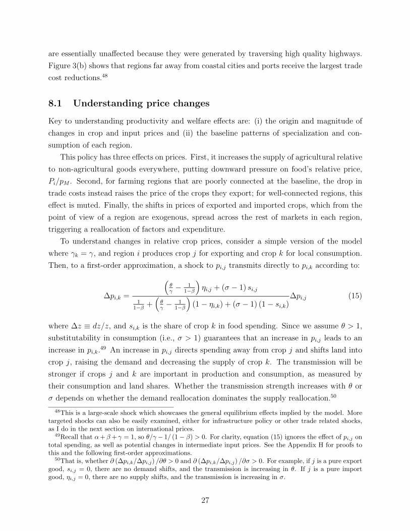
are essentially unaffected because they were generated by traversing high quality highways.

Figure 3(b) shows that regions far away from coastal cities and ports receive the largest trade

cost reductions.48

8.1 Understanding price changes

Key to understanding productivity and welfare effects are: (i) the origin and magnitude of

changes in crop and input prices and (ii) the baseline patterns of specialization and con-

sumption of each region.

This policy has three effects on prices. First, it increases the supply of agricultural relative

to non-agricultural goods everywhere, putting downward pressure on food’s relative price,

Pi/pM . Second, for farming regions that are poorly connected at the baseline, the drop in

trade costs instead raises the price of the crops they export; for well-connected regions, this

effect is muted. Finally, the shifts in prices of exported and imported crops, which from the

point of view of a region are exogenous, spread across the rest of markets in each region,

triggering a reallocation of factors and expenditure.

To understand changes in relative crop prices, consider a simple version of the model

where γk = γ, and region i produces crop j for exporting and crop k for local consumption.

Then, to a first-order approximation, a shock to pi,j transmits directly to pi,k according to:

∆pi,k =

(θγ− 1

1−β

)ηi,j + (σ − 1) si,j

11−β +

(θγ− 1

1−β

)(1− ηi,k) + (σ − 1) (1− si,k)

∆pi,j (15)

where ∆z ≡ dz/z, and si,k is the share of crop k in food spending. Since we assume θ > 1,

substitutability in consumption (i.e., σ > 1) guarantees that an increase in pi,j leads to an

increase in pi,k.49 An increase in pi,j directs spending away from crop j and shifts land into

crop j, raising the demand and decreasing the supply of crop k. The transmission will be

stronger if crops j and k are important in production and consumption, as measured by

their consumption and land shares. Whether the transmission strength increases with θ or

σ depends on whether the demand reallocation dominates the supply reallocation.50

48This is a large-scale shock which showcases the general equilibrium effects implied by the model. Moretargeted shocks can also be easily examined, either for infrastructure policy or other trade related shocks,as I do in the next section on international prices.

49Recall that α+ β+ γ = 1, so θ/γ− 1/ (1− β) > 0. For clarity, equation (15) ignores the effect of pi,j ontotal spending, as well as potential changes in intermediate input prices. See the Appendix H for proofs tothis and the following first-order approximations.

50That is, whether ∂ (∆pi,k/∆pi,j) /∂θ > 0 and ∂ (∆pi,k/∆pi,j) /∂σ > 0. For example, if j is a pure exportgood, si,j = 0, there are no demand shifts, and the transmission is increasing in θ. If j is a pure importgood, ηi,j = 0, there are no supply shifts, and the transmission is increasing in σ.

27

Comparative advantage, in the form of Ricardian differences in land productivity and

relative factor endowments, drives regional specialization. Within-region heterogeneity in

land quality, inversely related to θ, limits the degree of specialization. This pattern of

specialization is captured by land shares, ηi,k and consumption shares, si,k. In my baseline

quantification, expenditure is concentrated in a few crops (potatoes, rice, yellow maize, and

wheat), but the production allocations differ markedly across regions (see Appendix Table

L.17). Using equation (15), we then predict a strong demand-driven transmission of prices

among high-consumption goods, and from those goods to the rest. Further, we expect this

transmission to be correlated across regions.

8.2 Quantitative effects of the policy

Productivity Since each region can grow many crops, we need a multi-crop index of total

factor productivity, which regional value added provides.51 Moreover, to express TFP in

units that do not change across equilibria, I express this index in units of the intermediate

input at the port. We can then compute a simple expression for the first-order approximation

to the change in productivity

∆TFPi =1

1− βi

∑k

πi,k∆pi,k −βi

1− βi∆ρi. (16)

Productivity tends to increase when crops with large revenue shares become more valu-

able and when inputs become cheaper. Changes in revenue shares, however, do not have a

first-order effect on TFP (see Costinot and Vogel (2015)), although may drive changes in

equilibrium prices, as implicit in (15).

Without knowledge of the changes in prices, for which we need to compute the new

equilibrium, this formula can be applied directly only in special cases. For instance, suppose

a region exports all its output to the rest of the world, while it imports the intermediate input.

In that case, with the median trade cost reduction (∆d = −0.117) and average cost shares

(βi = .22), one predicts an increase in TFP of −(1 + βi

)/(1− βi

)∆d×100 = 18.3%. Of this

increase, about 1/6 is due to improved access to intermediate inputs (βi/(1− βi

)∆d×100).

This calculation also shows that, once prices are known, to a first-order approximation the

changes in productivity –and, later on, in welfare– are proportional to the reductions in trade

costs.52

Figure 6(a) relates regional productivity gains to changes in trade costs. The policy

51Further discussion of the properties of this index is provided in Appendix G.52However, as shown in Figure L.9, even when using the new equilibrium prices, when productivity gains

are large, equation (16) misses substantial gains due to factor reallocation across crops.

28

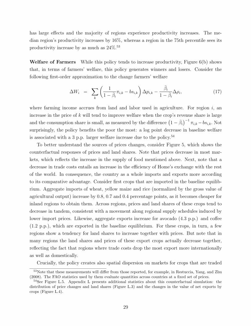
has large effects and the majority of regions experience productivity increases. The me-

dian region’s productivity increases by 16%, whereas a region in the 75th percentile sees its

productivity increase by as much as 24%.53

Welfare of Farmers While this policy tends to increase productivity, Figure 6(b) shows

that, in terms of farmers’ welfare, this policy generates winners and losers. Consider the

following first-order approximation to the change farmers’ welfare

∆Wi =∑k

(1

1− βiπi,k − bsi,k

)∆pi,k −

βi1− βi

∆ρi, (17)

where farming income accrues from land and labor used in agriculture. For region i, an

increase in the price of k will tend to improve welfare when the crop’s revenue share is large

and the consumption share is small, as measured by the difference(1− βi

)−1πi,k− bsi,k. Not

surprisingly, the policy benefits the poor the most: a log point decrease in baseline welfare

is associated with a 3 p.p. larger welfare increase due to the policy.54

To better understand the sources of prices changes, consider Figure 5, which shows the

counterfactual responses of prices and land shares. Note that prices decrease in most mar-

kets, which reflects the increase in the supply of food mentioned above. Next, note that a

decrease in trade costs entails an increase in the efficiency of Home’s exchange with the rest

of the world. In consequence, the country as a whole imports and exports more according

to its comparative advantage. Consider first crops that are imported in the baseline equilib-

rium. Aggregate imports of wheat, yellow maize and rice (normalized by the gross value of

agricultural output) increase by 0.8, 0.7 and 0.4 percentage points, as it becomes cheaper for

inland regions to obtain them. Across regions, prices and land shares of these crops tend to

decrease in tandem, consistent with a movement along regional supply schedules induced by

lower import prices. Likewise, aggregate exports increase for avocado (4.3 p.p.) and coffee

(1.2 p.p.), which are exported in the baseline equilibrium. For these crops, in turn, a few

regions show a tendency for land shares to increase together with prices. But note that in

many regions the land shares and prices of these export crops actually decrease together,

reflecting the fact that regions where trade costs drop the most export more internationally

as well as domestically.

Crucially, the policy creates also spatial dispersion on markets for crops that are traded

53Note that these measurements will differ from those reported, for example, in Restuccia, Yang, and Zhu(2008). The FAO statistics used by them evaluate quantities across countries at a fixed set of prices.

54See Figure L.5. Appendix L presents additional statistics about this counterfactual simulation: thedistribution of price changes and land shares (Figure L.3) and the changes in the value of net exports bycrops (Figure L.4).

29

only domestically, most importantly potatoes, which account for about 23% of consumption.

Equation (15) explains this adjustment as the net effect of two forces. The drop in the relative

price of high-consumption imports, like wheat and yellow maize, puts a downward pressure

on potato prices across the board (since si,k is large for k = wheat, maize and potato).

For regions that export potatoes to urban centers, this acts like a further price shock that

spreads to other crops. In contrast, the rise in the price of exports puts an upward pressure

in potato markets, mostly in regions that also produce avocado (since there ηi,k is large for

k = avocado and potato, and low for others).

Pulling together across crops, there is a 0.56 correlation between changes in prices and

land shares, which confirms the importance and correlation of demand shocks across regions.

Figure 5, however, also points out the large heterogeneity of the price adjustments, which

underlies the heterogeneity of changes in welfare and productivity.

Welfare of non-agriculture workers A simple way of assessing the impact of the policy

on net food buyers is to calculate the change in real non-farm income, wi,M/Pbi . Although

the changes are relatively small, Figure 6(c) shows that net food buyers gain the least (and

even lose), where the trade costs fall the most.

Paving roads when labor is mobile within regions To understand the implications

of a certain degree of labor mobility across sectors, I study an environment where worker

heterogeneity induces a positively sloping sectoral labor supply.55 I proceed in two steps.

First, I compute a new baseline equilibrium in which workers can move freely between agri-

culture and non-agriculture, but not across regions. Second, I calculate the welfare effects

of the policy relative to this new baseline. Doing so neutralizes the gains that accrue solely

from allowing for worker mobility. Note, however, that these results are only an illustration

of how the model works, since they imply counterfactual baseline labor allocations.

Figure 6(d) shows that changes in agricultural welfare are negatively related to changes in

trade cost, opposite to when workers cannot move. To understand why, consider a region with

a large underlying productivity advantage of non-manufacturing and high costs of trading

with the rest of the country. In a baseline equilibrium with labor mobility, this region employs

a large fraction of their workers in non-agriculture, and few as farmers. Wages reflect non-

agriculture productivity and food is expensive to induce some workers to produce it. If this

region becomes more integrated, the relative price of agricultural goods decreases in those

55The Appendix explains the details of the calibration. Intuitively, I choose parameters such that thewages in each region are the same as in the baseline calibration – using the model in Lagakos and Waugh(2013) – and let labor allocations adjust.

30

regions, pulled closer to urban and international prices. The income lost by farmers then

leads to a welfare decrease.

9 The Effect of an International Price Shock

I now study how a shock to international prices spreads throughout the domestic trade

network. As a concrete example, I feed in an international price shock in line with the effect

a Doha reforms scenario, according to World Bank’s simulations.56 The shock entails a mild

increase in the price of cereals and cotton, and a small decrease in the price of fruit crops.

On average farmers benefit (0.24% welfare gain), and non-farm workers lose (-0.04% wel-

fare loss). But this example also shows the importance of accounting for general equilibrium

effects in transmitting foreign shocks to domestic prices. With knowledge of the changes

in the equilibrium prices, the first-order approximation (17) turns out to be quite accurate

since the shock is relatively small (see Figure L.9(b) in the Appendix.) Figure 7 compares

these accurate predictions with those obtained by using the SOE assumption that interna-

tional prices apply directly to every regional market. While the predictions are positively

correlated, the SOE prediction gets the sign wrong about in 27% of the regions.

Domestic trade costs insulate regions far away from ports from shocks to international

prices. Thus, the price of rice, cotton, and maize increases as much as the international

price only close to ports, and much less elsewhere (see Figures L.6 and L.7 in the Appendix.)

In turn, these price shocks trigger displacements in the supply and demand of other crops

(equation 15). For example, the negative international shock to the price of bananas is

tempered in many regions as the supply of bananas shifts in due to the increased production

of cotton, yellow maize and rice; this mitigates the negative income effect of a drop in the

export prices. For other crops, like potatoes, prices increase almost everywhere, as consumers

substitute away from cereals (recall that the consumption share of cereals and potatoes is

high). This change in the price of potatoes benefits its producers, but hurts its consumers.

Note that the change in potato prices, although large, is entirely indirect because potato is

only traded domestically.

56I obtain the simulated changes in world prices reported in Hertel and Ivanic (2006). For each crop, Iaverage the import and export price changes for the World, relative to a bundle of rich country manufacturingexports (Tables 3.8 and 3.9 in Hertel and Ivanic (2006)). Then I classify the crops in my data accordingto their categories. The largest prices changes are for rice (7.7%), wheat (1.6%), other cereals (3.45%) andplant fibers (5.9%). I assume these price changes apply relative to the numeraire in my model.

31

10 Conclusion

The first message of this paper is that removing barriers to market access can have a posi-

tive effect on farmers’ productivity. Large-scale infrastructure shocks, however, can generate

winners and losers if crops are substitutes in production and consumption, in spite of the

possibility of land reallocation. Second, international shocks spread through regional markets

and have spatially heterogeneous impacts. In response to either shock, welfare and produc-

tivity depend on specialization and price adjustments, both of which the model interprets

through the lens of comparative advantage.

The framework I have presented can be used to answer other questions at the intersection

of development and trade. For example, since Engel’s Law is a prominent feature in the data,

augmenting the model with non-homothetic preferences can help shed light on how income

inequality shapes the urban-rural exchange.

References

Adamopoulos, T. (2011): “Transportation Costs, Agricultural Productivity, And Cross-

Country Income Differences,” International Economic Review, 52(2).

Adamopoulos, T., and D. Restuccia (2014): “The Size Distribution of Farms and

International Productivity Differences,” American Economic Review, 104(6), 1667–97.

Alvarez, F., and R. J. Lucas (2007): “General equilibrium analysis of the Eaton-Kortum

model of international trade,” Journal of Monetary Economics, 54(6), 1726–1768.

Arkolakis, C., A. Costinot, and A. Rodriguez-Clare (2012): “New Trade Models,

Same Old Gains?,” American Economic Review, 102(1), 94–130.

Atkin, D. (2013): “Trade, Tastes, and Nutrition in India,” American Economic Review,

103(5), 1629–63.

Behrman, J. R., and A. B. Deolalikar (1989): “Is Variety the Spice of Life? Implica-

tions for Calorie Intake,” The Review of Economics and Statistics, 71(4), 666–72.

Caliendo, L., and F. Parro (2015): “Estimates of the Trade and Welfare Effects of

NAFTA,” Review of Economic Studies, 82(1), 1–44.

Chaney, T. (2008): “Distorted Gravity: The Intensive and Extensive Margins of Interna-

tional Trade,” American Economic Review, 98(4), 1707–21.

32

Chomitz, K. M., and D. A. Gray (1996): “Roads, Land Use, and Deforestation: A

Spatial Model Applied to Belize,” The World Bank Economic Review, 10(3), 487–512.

Costinot, A., and D. Donaldson (2012): “Ricardo’s Theory of Comparative Advantage:

Old Idea, New Evidence,” American Economic Review, Papers and Proceedings, 102(3),

453–58.

(2014): “How Large are the Gains from Economic Integration? Theory and Evidence

from U.S. Agriculture, 1880-1997,” .

Costinot, A., D. Donaldson, and C. Smith (2016): “Evolving Comparative Advantage

and the Impact of Climate Change in Agricultural Markets: Evidence from 1.7 Million

Fields around the World,” Journal of Political Economy, 124, 205–248.

Costinot, A., and J. Vogel (2015): “Beyond Ricardo: Assignment Models in Interna-

tional Trade,” Annual Review of Economics, 7(20585), 31–62.

Deardorff, A. (1998): “Determinants of Bilateral Trade: Does Gravity Work in a Neo-

classical World?,” in The Regionalization of the World Economy, NBER Chapters, pp.

7–32. National Bureau of Economic Research, Inc.

Deaton, A. (1997): The analysis of household surveys: a microeconometric approach to

development policy. The World Bank.

Dekle, R., J. Eaton, and S. Kortum (2008): “Global Rebalancing with Gravity: Mea-

suring the Burden of Adjustment,” IMF Staff Papers, 55(3), 511–540.

Dias Avila, A. F., and R. E. Evenson (2010): Total Factor Productivity Growth in Agri-

culture: The Role of Technological Capitalvol. 4 of Handbook of Agricultural Economics,

chap. 72, pp. 3769–3822. Elsevier.

Dix-Carneiro, R. (2014): “Trade Liberalization and Labor Market Dynamics,” Economet-

rica, 82(3), 825–885.

Donaldson, D. (2015): “Railroads of the Raj: Estimating the Impact of Transportation

Infrastructure,” American Economic Review, Forthcoming.

Eaton, J., and S. Kortum (2002): “Technology, Geography, and Trade,” Econometrica,

70(5), 1741–1779.

Eaton, J., S. S. Kortum, and S. Sotelo (2012): “International Trade: Linking Micro

and Macro,” NBER Working Papers 17864, National Bureau of Economic Research, Inc.

33

Fajgelbaum, P., and S. Redding (2014): “External Integration and Internal Devel-

opment: Evidence from Argentina, 1870-1914,” NBER Working Papers 20217, National

Bureau of Economic Research, Inc.

Fajgelbaum, P. D., and A. K. Khandelwal (2016): “Measuring the Unequal Gains

from Trade,” The Quarterly Journal of Economics, p. Forthcoming.

Fieler, A. C. (2011): “Nonhomotheticity and Bilateral Trade: Evidence and a Quantitative

Explanation,” Econometrica, 79(4), 1069–1101.

Gollin, D., D. Lagakos, and M. E. Waugh (2013): “The Agricultural Productivity

Gap,” The Quarterly Journal of Economics.

Gollin, D., and R. Rogerson (2014): “Productivity, transport costs and subsistence

agriculture,” Journal of Development Economics, 107(C), 38–48.

Hayami, Y., and V. Ruttan (1985): Agricultural development: an international perspec-

tive, Johns Hopkins studies in development. Johns Hopkins University Press.

Head, K., and T. Mayer (2014): Gravity Equations: Workhorse, Toolkit, and Cook-

bookvol. 4 of Handbook of International Economics, chap. 3, pp. 131–195. Elsevier.

Helpman, E., M. Melitz, and Y. Rubinstein (2008): “Estimating Trade Flows: Trading

Partners and Trading Volumes,” The Quarterly Journal of Economics, 123(2), 441–487.

Hertel, T. W., and M. Ivanic (2006): “Assessing the World Market Impact of Multilat-

eral Trade Reforms,” in Poverty & the WTO. Impacts of the Doha Development Agenda.

Palgrave Macmilland and the World Bank.

Hummels, D. (2001): “Toward a Geography of Trade Costs,” .

IIASA/FAO (2012): Global Agro-ecological Zones (GAEZ v3.0). IIASA, Laxenburg, Austria

and FAO, Rome, Italy.

Lagakos, D., and M. E. Waugh (2013): “Selection, Agriculture, and Cross-Country

Productivity Differences,” American Economic Review, 103(2), 948–80.

Markusen, J. R. (2013): “Putting per-capita income back into trade theory,” Journal of

International Economics, 90(2), 255–265.

Melitz, M. J. (2003): “The Impact of Trade on Intra-Industry Reallocations and Aggregate

Industry Productivity,” Econometrica, 71(6), 1695–1725.

34

Mesquita Moreira, M., J. Blyde, C. Volpe, and D. Molina (eds.) (2013): Too far

to export: domestic transport cost and regional export disparities in Latin America and the

Caribbean. Inter-American Development Bank.

Ministerio de Transportes y Comunicaciones de Peru (2011a): Anuario Estadis-

tico 2011.

(2011b): “D.S. N 012-2013-MTC,” .

Ossa, R. (2014): “Trade Wars and Trade Talks with Data,” American Economic Review,

104(12), 4104–46.

Parro, F. (2013): “Capital-Skill Complementarity and the Skill Premium in a Quantitative

Model of Trade,” American Economic Journal: Macroeconomics, 5(2), 72–117.

Ramondo, N., and A. Rodriguez-Clare (2013): “Trade, Multinational Production, and

the Gains from Openness,” Journal of Political Economy, 121(2), 273 – 322.

Restuccia, D., D. T. Yang, and X. Zhu (2008): “Agriculture and aggregate produc-

tivity: A quantitative cross-country analysis,” Journal of Monetary Economics, 55(2),

234–250.

Shoven, J., and J. Whalley (1992): Applying General Equilibrium. Cambridge Univer-

sity Press.

Swiecki, T. (2014): “Intersectoral Distortions and the Welfare Gains from Trade,” Discus-

sion paper.

The World Bank (2007): World Development Report 2008 : Agriculture for Development.

The World Bank.

Tombe, T. (2015): “The Missing Food Problem,” American Economic Journal: Macroeco-

nomics, 7(3), 1–33.

Vollrath, D. (2011): “The agricultural basis of comparative development,” Journal of

Economic Growth, 16, 343–370.

35

11 Tables and Figures

Table 1: The Spatial Dispersion of Unit Values

Crop Region dummies Urban dummyF statistic R-sq Coefficient s.e

alfalfaasparagus 18.162 0.238 0.336 0.078avocado 367.949 0.528 0.363 0.008banana 225.344 0.362 0.123 0.003barley grain 10956.440 0.671 0.402 0.013cacao 45.761 0.555 0.302 0.092cassava 590.747 0.331 0.246 0.004coffee 234.443 0.560 0.194 0.022cotton branchdry bean 168.256 0.285 0.190 0.005grape 113848.500 0.293 -0.016 0.006maize (amilaceo)maize (choclo) 200.228 0.428 0.335 0.007maize (yellow hard)onion 98.850 0.110 -0.016 0.003orange 364.937 0.316 0.128 0.004potato 259.760 0.352 0.242 0.003rice 168.931 0.188 0.054 0.002tangerine 155.203 0.318 0.156 0.005wheat 231.343 0.663 0.604 0.007

Notes. Unit values are not available for crops that are not consumed directly by households. Inthat case, the corresponding row is empty.

Table 2: Distribution of Largest, Average and Median Land Shares across Regions

min 1st quartile median 3rd quartile maxlargest share 0.205 0.317 0.404 0.538 1.000average share 0.053 0.077 0.091 0.125 1.000smallest share 0.000 0.000 0.001 0.003 1.000

36

Table 3: Estimates of the Transportation Model

Constrained Road QualityModel Model

log effective distance βdist 0.356 0.482( 0.093) ( 0.068)

high quality λhi 1.000 1.000— —

low quality λlo 1.000 10.983— ( 3.964)

Intercept β0 0.208 -0.104( 0.042) ( 0.155)

N 333 333R-squared 0.446 0.596

Bootstrapped standard errors in parentheses

Table 4: Summary Statistics of the Estimates of Iceberg Trade Costs, dni,k

mean std 10% 25% 50% 75% 90% max

iceberg 2.34 0.42 1.85 2.08 2.32 2.54 2.77 4.37

37

Figure 1: Four Motivating Facts(a) Coffee prices in space (in LCU) (b) Coffee prices decline with distance to Lima

(c) Number of crops grown by region (d) Average revenue per unit of land

(e) Roads and geography in Peru

Notes. Panels (a) and (b) use average prices, over 2008-2011. Blank regions indicate the coffee is not grownthere. “Road distance” is calculated using the road network. Panel (e) Peru’s road system is divided in threelevels: National, Departmental and Neighborhood roads (only the first two are plotted, to avoid clutter.)

38

Figure 2: Estimation of technology parameters(a) Cost shares of land across crops γk (b) Identification of inverse heterogeneity θ

Figure 3: Trade Costs in Space(a) Baseline iceberg trade cost to Lima (b) Average reduction in iceberg trade costs (%)

39

Figure 4: Fitting Price and Land Allocation Data at the Baseline(a) Farm-gate prices (crop means removed) (b) Land shares

Figure 5: Counterfactual Change in Prices and Land Shares: Roads paved

40

Figure 6: Counterfactual Change in Productivity and Welfare(a) Agricultural productivity (b) Agricultural welfare

(c) Non-agricultural welfare (d) Agricultural welfare (mobile labor)

Figure 7: Welfare Change following an International Price Shock (Model and SOE approximation)

41