DOLPi – A Low-Cost, RasPi-based Polarization Camera

©2015 by David Prutchi, Ph.D.

DOLPi – A Low-Cost, RasPi-based Polarization Camera

A polarimetric imager to detect invisible pollutants, locate landmines and IEDs, identify cancerous tissues, and maybe even observe cloaked UFOs.

David Prutchi, Ph.D.

Clouds of colorless pollutants, antipersonnel mines, and skin cancers are so difficult to detect because they blend so naturally with their background that our unaided eyes cannot see them1. However, an octopus faced with the same problem would probably have a very easy time at locating these threats. This is because our human eyes can only distinguish objects from their background through the contrast in their color and/or intensity. On the other hand, octopuses would be able to see the contrast in light polarization between these items and their background.

Try this experiment - next time that you go outdoors on a sunny day, tilt your head while wearing polarized sunglasses. You will find that parts of the sky turn into a lighter shade of blue when you turn your head sideways. The intensity of the glare will also change considerably as you tilt your head while looking at a reflective surface like still water, or the windshield of a car. Look at a static scene like a parking lot while tilting your head back and forth – do the windows of parked cars seem to flash? The reason for this phenomenon is that the light scattered by the sky, or reflected by many surfaces is “polarized”. That is to say that light waves from these sources vibrate mainly in one direction – more on this later.

In fact, every photon that reaches our eyes has its own polarization, yet this aspect of light is barely used in our daily life because our unaided eyes are insensitive to polarization2, and thus we don’t have an intuitive sense for its use.

In spite of this, polarization of light carries interesting information about our visual environment of which we are usually unaware. Some animals have evolved the capability to see polarization as a distinct characteristic of light, and rely critically on this sense for navigation and survival. For example, many fish, amphibians, arthropods, and octopuses3 use polarization vision as a compass for navigation, to detect water surfaces, to enhance the detection of prey and predators, and probably also as a private means to communicate among each other.

While we have used technology to expand our vision beyond the limits of our ordinary wavelength and intensity sensitivities, the unintuitive nature of polarization has slowed down the development of 1 You’ll have to keep on reading to find the reference about observing cloaked UFOs. 2 Humans have very marginal sensitivity to polarized light as discovered by Haidinger in 1846, but changes in polarization can only be perceived under very specific conditions. 3 “Octopuses” is the correct plural of “octopus.”


practical applications for polarization imaging. Polarization cameras do exist, but at over $50,000, they are mostly research curiosities that have found very few practical uses outside the lab.

The DOLPi project4 aims to widely open the field of polarization imaging by constructing a very low cost polarization camera that can be used to research and develop game-changing applications across a wide range of fields – spanning all the way from environmental monitoring and medical diagnostics, to security and antiterrorism applications.

The DOLPi polarization camera is based on a standard Raspberry Pi 2 single-board computer and its dedicated 5MP camera. What makes the DOLPi unique is that the camera sits behind a software-controlled electro-optic polarization modulator, allowing the capture of images through an electronic polarization analyzer. The modulator itself is hacked from a low-cost auto-darkening welding mask filter ($9 on eBay®). In spite of its simplicity, DOLPi produces very high quality polarization images such as the one shown in Figure 1.

This is a first-of-its-kind project! I am not aware of any polarization imager ever presented as an enthusiast-level DIY project, yet it holds truly awesome disruptive power for the development of brand new scientific and commercial applications!

Figure 1 - In spite of its simplicity and low cost, DOLPi produces very high quality images. Here is a screen capture of DOLPi viewing a few pieces of back-illuminated polarizing film. Unpolarized light shows as grayscale, while only polarized light is given a color representative of the angle of polarization.

4 Although DoLP refers only to the Degree of Linear Polarization, I liked the name DOLPi as a combination of DOLP and Pi (for Raspberry Pi). The logo is a one-eyed octopus (squids have polarization-sensitive eyes) with “Pi” as its tentacles.


Figure 2 – The DOLPi camera is fully self-contained so it can be easily taken wherever needed to perform high-quality polarization imaging, rendering not only the images corresponding to the linear Stokes parameters, but also to Polarization Intensity, Degree of Linear Polarization, Angle of Polarization, and their HSV rendering.

Polarization and Polarizers Polarization is an important characteristic of light that stems from its nature as an electromagnetic wave. In 1860, Scottish physicist James Clerk Maxwell figured out that an electric field that varies along space generates a magnetic field that varies in time and vice versa. For that reason, as an oscillating electric field generates an oscillating magnetic field, the magnetic field in turn generates an oscillating electric field, and so on. These oscillating fields together form the electromagnetic wave shown in Figure 3. In a wave of polarized light, like the one shown in the figure, the electric field is oscillates in one plane, while the magnetic field oscillates on a perpendicular plane. The wave travels at the speed of light along the line formed by the intersection of those planes. The electromagnetic wave shown in this figure is said to be “vertically polarized” because the electric field oscillates vertically in the frame of reference that we have chosen.


Figure 3 - An oscillating electric field generates an oscillating magnetic field, the magnetic field in turn generates an oscillating electric field, and so on. These oscillating fields together form an electromagnetic wave with wavelength λ that propagates at the speed of light. Adapted with permission from D. Prutchi and S.R. Prutchi, Exploring Quantum Physics through Hands-On Projects, John Wiley & Sons, Inc., 2012.

Light from most natural sources contains waves with electric fields oriented at random angles around its direction of travel. A wave of a specific polarization can be obtained from randomly-polarized light by using a polarizer filter. As shown in Figure 4, a polarizer can be made of an array of very fine wires arranged parallel to one another. The metal wires offer high conductivity for electric fields parallel to the the wires, essentially “shorting them out” and producing heat. Because of the nonconducting spaces between the wires, no current can flow perpendicularly to them. As such, electric fields perpendicular to the wires can pass unimpeded. In other words, the wire grid, when placed in a randomly-polarized beam, drains the energy out of one component of the electric field and lets its perpendicular component pass with no attenuation at all. Thus, the light emerging from the polarizer has an electric field that vibrates in a direction perpendicular to the wires.

Figure 4 - A parallel-wire polarizer absorbs electric-field lines that are parallel to the wires. Only the perpendicular electrical field component of light is allowed to pass, producing light that is polarized perpendicularly to the direction of the wires. Adapted with permission from D. Prutchi and S.R. Prutchi, Exploring Quantum Physics through Hands-On Projects, John Wiley & Sons, Inc., 2012.


Although the wire-grid polarizer is easy to understand, it is useful only down to certain wavelengths because the wires have to be a fraction of the wavelength apart. This is difficult and expensive to do for short wavelengths such as those of visible light5. In 1938 E. H. Land invented the H-Polaroid sheet, which acts as a chemical version of the wire grid. Instead of long thin wires it uses long thin polyvinyl alcohol molecules that contain many iodine atoms. These long, straight molecules are aligned almost perfectly parallel to one another. Because of the conductivity provided by the iodine atoms, the electric vibration component parallel to the molecules is absorbed. The component perpendicular to the molecules passes on through with little absorption.

Figure 5 – The amount of polarized light that passes through a polarizer depends on the angle between the polarized light’s axis and the polarizer’s main axis. a) The intensity of the light exiting the polarizer follows the cosine square of the angle between the light’s polarization axis and the polarizer’s main axis. With light going through two pieces of polarizer, minimum attenuation happens when the axes of polarization of the pieces of film are aligned (b). Attenuation increases as the angle between the axes increases (c) until a maximum attenuation occurs when the films are cross-polarized.

The amount of polarized light that passes through a polarizer depends on the angle between the polarized light’s axis and the polarizer’s main axis. As shown in Figure 5, the intensity of the light exiting

5 Wire-grid polarizers can now be made with lithography techniques and are used as part of micropolarizer arrays. See Figure 32-c.


the polarizer follows the cosine square of the angle between the light’s polarization axis and the polarizer’s main axis. Two polarizers in series will attenuate non-polarized light by an amount dependent on the rotation between the polarizers. Maximum transmission will happen when the

polarizers are aligned ( 2cos (0 ) 1° = ), while minimum transmission will take place with the polarizer

orientations crossed ( 2cos (90 ) 0° = ). Half of the maximum intensity is observed at a rotation angle of

45⁰.

Besides linear polarization, light can also be circularly polarized. This type of polarization is obtained when light polarized at 45⁰ passes through a material that transmits light at different speeds depending on its polarity. Linear polarization is thus given a “twist” when one polarization component (e.g. the vertical component of the 45⁰ light) is retarded by ¼ of its wavelength with respect to the other component (e.g. the horizontal component). When exiting the retarder material, the vertical component is slowed down so that it is out of phase with the horizontal component. To an observer receiving this light, the electric field will appear to rotate rather than just oscillate up and down. Hence the term “circular” polarization. As shown in Figure 6, circularly-polarized light can be polarized either clockwise or counterclockwise.

Figure 6 – Circularly-polarized light. The convention is to define the sense of polarization as viewed by the receiver, so (a) represents the electric field vector as a function of time of right-handed, clockwise circularly polarized light, while (b) represents left-handed, clockwise circularly polarized light.

The Polarization Modulator At the heart of the DOLPi camera is the Electro-Optic (EO) polarization modulator. This assembly, which consists of two liquid-crystal panels and a linear polarizer film, selectively passes light at different polarization angles under software control.

The liquid crystal panel used for the DOLPi camera is harvested from a low-cost auto-darkening welding mask filter (Figure 7). These are similar in construction to an LCD display, where the whole filter is a single gigantic “pixel”. In its intended use, the auto-darkening filter allows the user to see through the


filter while setting up the pieces to be welded, but as soon as light sensors detect the welding arc, the filter turns dark to protect the welder’s eyes.

Figure 7 – The liquid crystal panel (LCP) for the DOLPi camera is harvested from a low-cost auto-darkening welder mask filter. I purchased these units for $9 each on eBay®. The box in which the filter came indicates that it is manufactured by “Mask” in China. Their website is www.auto-mask.com. b) The front side of the filter’s enclosure (facing the pieces being welded) exposes the UV/IR filter that preceded the electrically-controlled light shutter, two photovoltaic panels (“solar cells”), and two light sensors used by the circuit to detect the presence of a welding arc.

The electrically-controlled light shutter in the auto-darkening filter is based on a liquid crystal panel (LCP) sandwiched between two polarizers. The liquid crystal panel is constructed from two glass windows separated a few microns apart. Each window is coated with transparent conductive Indium Tin Oxide (ITO) that will serves as an electrode. Depending on the type of liquid crystal used, a thin dielectric layer may then applied over the ITO and gently rubbed to provide for liquid crystal molecular alignment. The cavity is then filled with birefringent nematic liquid crystal material6. Lastly, electrical contacts are attached and the panel is environmentally sealed.

As shown in Figure 8-a, with no bias voltage applied between the electrodes, the liquid crystal molecules are guided by the scratch lines rubbed to form the alignment layer, and thus align parallel to the windows. In this orientation the liquid crystal panel shifts the polarization of incoming light by (approximately) 90⁰. However, as shown in Figure 8-b, when 5V are applied to the panel, the liquid crystal molecules align with the electric field and tip perpendicular to the windows. In this state, the polarization of incoming light remains largely unchanged (i.e. polarization shift is approximately 0⁰).

6 “Liquid crystals” are matter in a state that has properties between those of conventional liquid and those of solid crystal.

http://www.auto-mask.com/


Figure 8 –Without a voltage applied to the LCP, the liquid crystal molecules have an ordered orientation, which together with the stretched shape of the molecules causes them to shift the polarization of light by 90⁰ (a). When an electric field is applied, the molecules align to the field and the polarization shift depends on the tilting of the liquid crystal molecules. Beyond some voltage, the LCP introduces almost no polarization tilt (b).

Figure 9 shows how the electrically-controlled light shutter in the auto-darkening filter works. Light from the scene is polarized by a first polarizer film. In the absence of the LCP, the polarized light would not be able to go through the second polarizer because it is set orthogonally with respect to the first polarizer. However, when the unbiased LCP is placed in the middle, it rotates the polarization of the light passing through the first polarizer by 90⁰ such that it can go through the second polarizer. However, to darken the filter, the mask’s control circuit applies >5V to the LCP, which causes light going through it to maintain the polarization set by the first polarizer, thus preventing the light to go through the second polarizer and into the welder’s eyes.


Figure 9 – The core component of the auto-darkening welding mask filter is a liquid crystal panel (LCP) sandwiched between two crossed polarizers. a) In the absence of an electric field, the LCP turns the polarization by 90⁰, so light can go through the the second polarizer unimpeded. b) When 5V are applied across the LCP, polarization is conserved, so light cannot pass through the second polarizer. c) Transmission curve for the filtered, electrically-controlled light attenuator of the auto-darkening welding mask filter. Without the UV/IR filter (purple glass cover) the transmission at 0V is around 30% and drops to around 1% at 5V.

As shown in Figure 10, opening the plastic enclosure is easy. The two half-shells forming the enclosure are glued together and can be separated with a blade or screwdriver. The LCP’s drive wires can then be unsoldered (or cut) from the circuit.


One side of the electro-optical assembly is purple, while the other is green. The purple glass is a filter that cuts out infrared and ultraviolet emissions from reaching the welder’s eyes. This filter also cuts out some of the light reaching the polarizers and LCP. It can be removed with ease by cutting the bit of transparent tape on the sides and lifting it with a sharp razor. Without this filter, the unbiased optical attenuator passes around 30% of incoming light, and darkens to allow only 1% of the light through at a drive voltage of 5V. Go ahead – connect a variable-voltage power supply to the assembly and play with it. You should see that it lets light through up to around 1.5V when it starts to darken, reaching full attenuation at around 3.6V. The panel should tolerate voltages of around 10V with no damage.

Figure 10 – Teardown of the auto-darkening welding mask filter. The electrically-controlled light shutter and its control circuit can be removed by prying apart the two half shells that form the plastic enclosure.

Polarization Imaging One last step before being able to use the LCP for imaging is to remove the back-side polarizer film. It peels off easily after lifting a corner with a sharp hobby knife. The remaining polarizer and LCP now form a voltage-controlled polarization analyzer. Let’s call this assembly a “VCPA” for short. It is important to note that the polarizing film used in auto-darkening welding masks is oriented at 45⁰ with respect to the edges of the LCP.

A very simple, yet interesting first experiment in polarization imaging can already be conducted at this stage with the VCPA. All you’ll need besides the VCPA assembly is a 3Hz square-wave signal generator. An example circuit is shown in Figure 11.


Now, LCPs are commonly not operated with DC voltages for extended periods of time because DC polarization degrades the liquid crystal. In fact, critical-use drivers should be no net DC bias present in the drive signal in order to prevent ion migration within the LCP which impairs its performance and lifetime. Instead, LCPs should be driven with alternating current in the few kHz range. The LCP will respond to the RMS voltage across its electrodes. The LCP in the auto-darkening welding mask filter that I used is DC-driven, so this LCP may be DC-tolerant, but my recommendation is not to use the driver of Figure 11 for long periods of time.

Take the polarizer film that you pulled before from the assembly and set it some distance away from you. Now look at the scene through the VCPA (with the polarizer facing your eyes). While most of the scene should remain steady, the piece of polarizer will appear flashing when viewed through the VCPA. Try looking at items that include an LCD display (e.g. computer monitor, smartphone, calculator, etc.), as well as a piece of plastic reflecting sunlight through this device. Even with this simple gadget you should be able to appreciate the potential of adding polarization information to our regular color/intensity vision!

Figure 11 – A simple 555-based square-wave oscillator can be used to drive the VCPA at a frequency of around 3Hz. Materials that reflect polarized light appear to flash brightly when viewed through this device.

Boyd B. Bushman (of Area 51 UFO “deathbed confession” fame) described in a 1995 Patent (U.S. Patent 5,404,225) what essentially amounts to binoculars fitted with a VCPA to help detect man-made (or alien?7) objects, such as military vehicles and high-voltage power lines. The idea is that since these

7 I have to wonder if the true background behind this line of Boyd Bushman’s research related more to his personal fascination with UFOs than with any true Lockheed military project.

U1 LM555

OUT3

RST4

VCC8

GND1

CV5

TRG2 THR6

DSCHG7

C10.01uF

+5V

+ C210uF

R1100k

R210k

LCP

FrequencyVCPA

Polarizer film


objects incorporate plenty of glass, plastic, paints, rubbers, and other materials that polarize light, they look different through a polarizer that is set at different angles. When viewed through the oscillator-driven VCPA, such materials will appear to flash.

Since most natural backgrounds do not show the polarizing contrast between angles of polarization, changing the angle of the polarization analyzer will not cause natural objects and background to vary. Only polarizing materials and surfaces will be highlighted, making targets stand out, giving away their location. Bushman reported that neither camouflage nor moderate foliage stops the systems from highlighting man-made targets because adequate flashing can still be observed.

Figure 12 – Man-made objects are easier to discriminate from a natural background if polarization information is used to supplement the image. A 1995 patent describes a pair of binoculars that incorporate a switching polarization analyzer to highlight military targets by making them flash against a steady background.

The same concept can be applied to polarization imaging with a camera, in which case the degree of polarization can be encoded by subtracting the image obtained with one polarization from a frame acquired with the polarization analyzer set at the orthogonal polarization. Of course, switching of the polarization analyzer in this case must be done synchronously with the camera’s scan. This is the operating principle of the “Samba” polarimetric camera made by Bossa Nova Technologies of Culver City, CA., which provides “polarization contrast” images at video rate.

Polarization analysis with a single VCPA is known as “incomplete” because it cannot differentiate light polarized at 45⁰ with respect to the polarizer film in the VCPA as being polarized. Looking back at Figure 5-c we can see that light polarized at 45⁰ will look the same whether the analyzer is set to 0⁰ or 90⁰. To deal with this condition, Bossa Nova Technologies added an optical component known as a “quarter-wave plate” and a second liquid crystal cell to rotate polarization by 45⁰. Their “Salsa” camera is this able to perform “complete” linear polarization analysis by switching both liquid-crystal plates through all four combinations to yield images analyzed at -45⁰, 0⁰, 45⁰, and 90⁰ [Vedel et al., 2011; Lefaudeux, 2011]. This system uses custom-made ferroelectric liquid crystals mounted directly in front of the camera’s CCD to achieve excellent linearity at 28 polarization frames per second at 320x240 resolution, or 8.75 frames per second at 782x582 pixel resolution.


Figure 13 – Bossa Nova’s Salsa camera achieves complete polarization imaging by switching a liquid-crystal quarter-wave plate preceded by a fixed quarter-wave plate, and a liquid-crystal half-wave plate followed by a linear polarizer through all four liquid-crystal setup combinations to yield video images containing information from individual frames analyzed at -45⁰, 0⁰, 45⁰, and 90⁰.

The DOLPi Camera Bossa Nova’s method is straightforward if laboratory optical-grade components are used. These are very expensive and out of reach for most private enthusiasts. However, I found through experimentation that a welding mask LCP and a polarizer sheet can also give very satisfactory results.

The welding mask’s LCP can be made to rotate polarization to values between its two extremes at 0⁰ and 90⁰. Although it is possible to find a voltage that will set the LCP to rotate light’s polarization by around 45⁰, changes in the liquid crystal take place with time, so the polarization state will shift with complex, interacting time constants that are dependent on temperature, age, and other factors. For this reason, the drive amplitude to achieve 45⁰ rotation of polarization needs to be periodically recalibrated.

This is a good place to state that not all liquid-crystal shutters are suitable for conversion into LCPAs that can be driven to analyze at 45⁰. I tested modified light shutters from 3D active glasses made for the Sony Playstation, as well as some low-cost universal 3D glasses for DLP projector units (“model G15-DLP”) without success. The issue with these is that their liquid crystal panels have only two stable states (0⁰ and 90⁰) with an extremely sharp transition zone that does not lend itself to intermediate polarization states. At the same time, I would like to mention that the only welding mask filter that I have tried is the one shown in Figure 7, and I don’t know if LCPs from other auto-darkening welding mask filters would work equally well.

Figure 16 shows a block diagram for the DOLPi camera, which is my solution to acquiring the three pictures (analyzed at 0⁰, 45⁰, and 90⁰) to perform complete linear polarization imaging of a scene. The imaging element is the official Raspberry Pi camera connected directly to a Raspberry Pi 2’s dedicated camera connector. The camera views the scene through the VCPA hacked from an auto-darkening


welding mask filter as discussed above. In my first prototype (Figure 20), I chose to tilt the VCPA by 45⁰ with respect to the camera’s horizon because the polarizer film used in the mask is oriented at this angle, so tilting reorients it vertically with respect to the camera. However, as you will soon realize, identical results are possible when mounting the LCPA horizontally, vertically, or at 45⁰ by defining the correct frame of reference through software.

As discussed before, liquid crystal panels should not be operated with DC for prolonged periods of time, but if you want to first see what the camera can do before building a more complex AC driver with self-calibration, you can start by assembling the really simple circuit of Figure 14. The GPIO pins refer to the Raspberry Pi 2’s GPIO interface.

When GPIO pin 21 and GPIO pin 22 are low, both LCP electrodes are at the same potential, and thus the LCP causes a polarization shift of 90⁰. When GPIO 22 is high, the LCP is biased at +5V (minus a diode drop), causing no rotation in polarization (0⁰). When GPIO 22 is low and GPIO 21 is set high, the LCP is biased at a voltage determined by potentiometer R1, which is manually set to produce maximum contrast in the DOLPi image between polarizers oriented at 45⁰ and -45⁰.

Figure 14 – The Raspberry Pi can drive the VCPA through this simple circuit to analyze at 0⁰, 45⁰, and 90⁰. The voltage used to analyze at 45⁰ is selected manually via potentiometer R1. This circuit imposes DC polarization across the LCP, so it shouldn’t be used for extended periods of time. However, it will quickly get you playing with polarimetric imaging until you get around to building the AC driver (Figure 17).

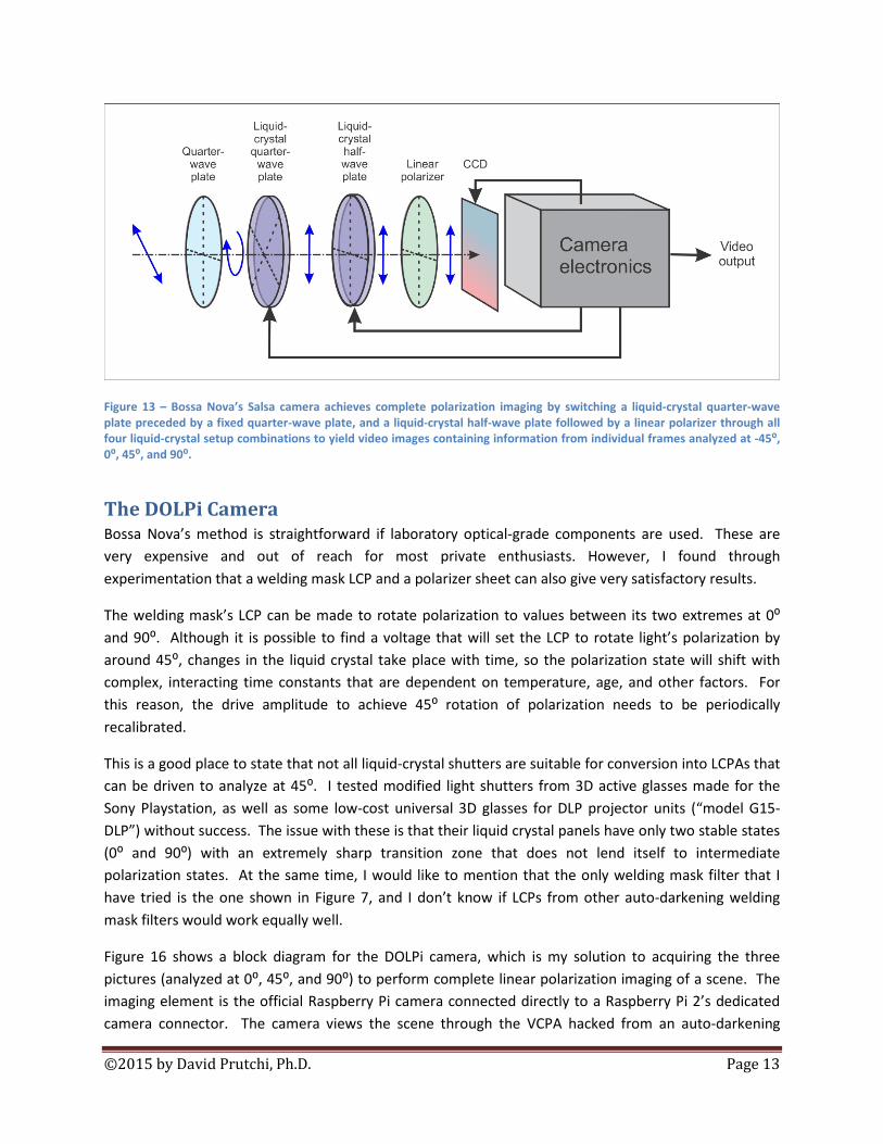
The Python listing for this simple polarization camera is shown in Table 1. Figure 15 shows a simplified flowchart for the software. The program first imports necessary packages and then allows the camera to sample the scene before locking its exposure settings. The imaging loop consists of taking three grayscale images with the VCPA set at 0⁰, 45⁰, and 90⁰, and then combining these pictures into a single color image encoding the scene’s intensity and polarization.

Polarizer

LCP

GPIO 21 R110k

D2

1N4001GPIO 22

45 degrees

O degrees

RPi Camera BusRPi Camera

D1

1N4001

R2100k


Figure 15 - This flowchart explains the simple software used to image with the camera of Figure 14. After loading libraries and initializing the Raspberry Pi’s ports, the Raspberry camera is allowed to sample the scene for a few seconds to set its internal auto-exposure and then locking the exposure settings to keep consistency among images. The imaging loop consists of taking three grayscale images with the VCPA set at 0⁰, 45⁰, and 90⁰, and then combining these pictures into a single color image that encodes polarization.

Table 1 – DOLPiManual.py Python code

# DOLPiManual.py # # This Python program demonstrates the DOLPi polarimetric camera # under manual control (potentiometer setting for analyzer at 45 degrees) # # (c) 2015 David Prutchi, Ph.D., licensed under MIT license # (MIT, opensource.org/licenses/MIT) # # This version uses a voltage-controlled polarization analyzer (VCPA) that # consists of a liquid crystal panel(LCP) and a polarizer film. The polarizer # film is placed between the LCP and camera.


# The VCPA is driven by GPIO pins 22 and 23 (via diodes and a pot) to 3 states: # 1. 5V for no rotation of polarization # 2. ~45 degrees of rotation as set by potentiometer # 3. 0V for 90 degrees of rotation # #import the necessary packages from picamera.array import PiRGBArray from picamera import PiCamera import time import cv2 import RPi.GPIO as GPIO import numpy as np #IO PINS #------- dc0degpin=22 #0 degree VCPA DC bias manual mode dc45degpin=21 #45 degree VCPA DC bias manual mode GPIO.setwarnings(False) #Don't issue warning messages if channels are defined GPIO.setmode(GPIO.BCM) GPIO.setup(dc0degpin,GPIO.OUT) GPIO.setup(dc45degpin,GPIO.OUT) GPIO.output(dc0degpin,False) GPIO.output(dc45degpin,False) #Raspberry Pi Camera Initialization #---------------------------------- #Initialize the camera and grab a reference to the raw camera capture camera = PiCamera() camera.resolution = (640, 480) #camera.resolution = (1280,720) camera.framerate=80 rawCapture = PiRGBArray(camera) camera.led=False #Auto-Exposure Lock #------------------ # Wait for the automatic gain control to settle time.sleep(2) # Now fix the values camera.shutter_speed = camera.exposure_speed camera.exposure_mode = 'off' gain = camera.awb_gains camera.awb_mode = 'off' camera.awb_gains = gain #Initialize flags loop=True #Initial state of loop flag


first=True #Flag to skip display during first loop video=True #Use video port? Video is faster, but image quality is significantly #lower than using still-image capture while loop: #grab an image from the camera at 0 degrees GPIO.output(dc0degpin,True) GPIO.output(dc45degpin,False) time.sleep(0.05) rawCapture.truncate(0) camera.capture(rawCapture, format="bgr",use_video_port=video) image0 = rawCapture.array # Select one of the two methods of color to grayscale conversion: # Blue channel gives better polarization information because wavelengt # range is limited # True grayscale conversion gives better gray balance for non-polarized light R=image0[:,:,1] #Use blue channel #R=cv2.cvtColor(image0,cv2.COLOR_BGR2GRAY) #True grayscale conversion #grab an image from the camera at 45 degrees GPIO.output(dc0degpin,False) GPIO.output(dc45degpin,True) time.sleep(0.05) rawCapture.truncate(0) camera.capture(rawCapture, format="bgr",use_video_port=video) image45 = rawCapture.array #Capture image at 45 degrees rotation # Select one of the two methods of color to grayscale conversion: # Blue channel gives better polarization information because wavelengt # range is limited # True grayscale conversion gives better gray balance for non-polarized light G=image45[:,:,1] #G=cv2.cvtColor(image45,cv2.COLOR_BGR2GRAY) #grab an image from the camera at 90 degrees GPIO.output(dc0degpin,False) GPIO.output(dc45degpin,False) time.sleep(0.05) rawCapture.truncate(0) camera.capture(rawCapture, format="bgr",use_video_port=video) # Select one of the two methods of color to grayscale conversion: # Blue channel gives better polarization information because wavelengt # range is limited # True grayscale conversion gives better gray balance for non-polarized light image90 = rawCapture.array #Capture image at 90 degree rotation B=image90[:,:,1] #B=cv2.cvtColor(image90,cv2.COLOR_BGR2GRAY) imageDOLPi=cv2.merge([B,G,R]) cv2.imshow("Image_DOLPi",cv2.resize(imageDOLPi,(320,240),interpolation=cv2.INTER_AREA))


#Display DOLP image GPIO.output(dc0degpin,False) GPIO.output(dc45degpin,False) k = cv2.waitKey(1) #Check keyboard for input if k == ord('x'): # wait for x key to exit loop=False # Prepare to leave cv2.imwrite("image0.jpg",image0) cv2.imwrite("image90.jpg",image90) cv2.imwrite("image45.jpg",image45) cv2.imwrite("RGBpol.jpg",cv2.merge([B,G,R])) cv2.imwrite("image0g.jpg",R) cv2.imwrite("image90g.jpg",G) cv2.imwrite("image45g.jpg",B) cv2.destroyAllWindows() quit

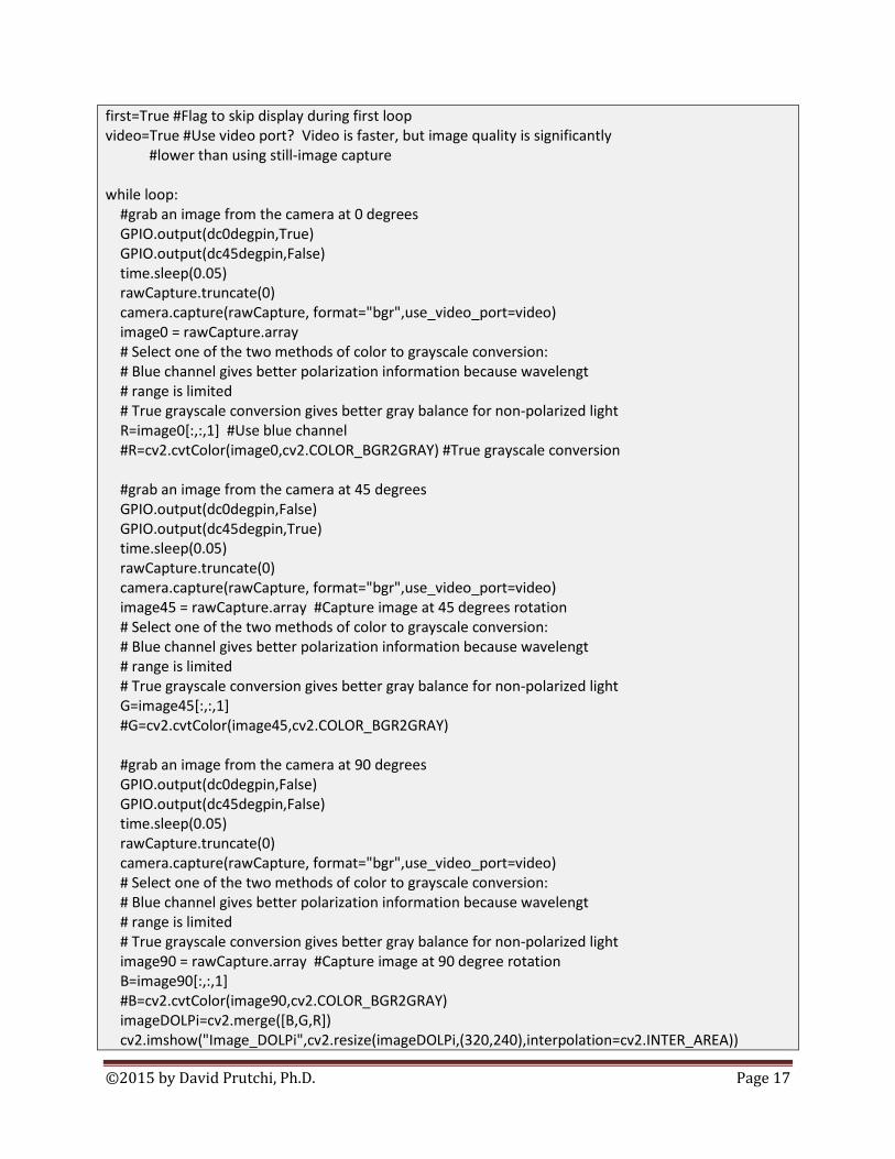
Now that you had a peek preview of DOLPi’s capabilities, go ahead and build DOLPi with its proper AC driver and auto-calibration. A block diagram is shown in Figure 16. The VCPA is driven with 2 kHz square-wave AC. The signal is generated by a 555-based square wave oscillator and fed to an AC-coupled amplifier through a voltage-controlled resistor implemented from a simple P-type JFET. The amplifier boosts the drive signal to a maximum peak-to-peak amplitude of 10V. The Raspberry Pi controls the amplitude of the drive signal through a MCP4725 digital-to-analog converter (DAC or D/A).

I built a self-calibrating mechanism for the camera by adding a blue LED, a 45⁰ polarizer, and a light sensor (a light-dependent resistor – or LDR) on a separate optical path across the VCPA. Before each use, the Raspberry Pi turns on the LED and measures the 45⁰-polarized light transmitted across the VCPA as the drive amplitude is ramped up. An ADS1015 12-bit, 4-channel analog-to-digital converter (ADC or A/D) is used by the Raspberry Pi to generate a transmission plot from which the D/A setting for maximum transmission can be found. The maximum value corresponds to the drive setting to be used to acquire images at an analysis angle of 45⁰. By the way, you can try connecting the DAC’s output directly to the LCP. The auto-calibration system should work if you want to DC-drive the LCP from the DAC and thus avoid constructing the AC driving circuit, but please keep in mind the possibility that this will deteriorate the LCP.


Figure 16 –Block diagram of the DOLPi camera. The VCPA is AC-driven at 2kHz. The drive amplitude is controlled from software via a D/A converter. The drive amplitude for 45⁰ polarization shift is determined by an auto-calibration circuit consisting of an A/D converter that measures the intensity of 45⁰ polarized light that goes through the VCPA as a function of D/A output.

Table 2 – Bill of Materials for DOLPi (some may be replaced or are optional)

Component reference Component/Material Source RasPi Raspberry Pi 2 - Model B - ARMv7 with

1G RAM Adafruit ID:2358

SD Card SanDisk SAEMSD64GBU3 64GB Extreme UHS-I microSDXC Memory Card (U3/Class 10)

B&H Photo

Keyboard/Mouse Miniature Wireless USB Keyboard with Touchpad

Adafruit ID:922

RasPi Camera Raspberry Pi Camera Board Adafruit ID:1367 PiTFT PiTFT Plus 480x320 3.5" TFT +

Touchscreen for Raspberry Pi (Pi 2 and Model A+ / B+)

Adafruit ID:2441

VCPA VCPA hacked from auto-darkening welding mask filter per text

Online (Amazon, eBay, etc). Filter manufactured by “Mask” www.auto-mask.com (see Figure 7)

ADC ADS1015 Breakout Board - 12-Bit ADC - 4 Channel with Programmable Gain Amplifier

Adafruit ID:1083

DAC MCP4725 Breakout Board - 12-Bit DAC w/I2C Interface

Adafruit ID:935

Battery Pack USB Battery Pack for Raspberry Pi - Adafruit ID:1565




4400mAh - 5V @ 1A Power Switch Breadboard-friendly SPDT Slide Switch Adafruit ID:805 GPIO Stacking Header Stacking Header for Pi A+/B+/Pi 2 -

2x20 Extra Tall Header Adafruit ID:1979

D1 Diffused blue LED Adafruit ID:780 R7 CdS photoresistor Adafruit ID: 161 U1 TLC555CP LinCMOS 555 timer IC Digikey 296-1857-5-ND Q1 J112 small-signal P-type JFET Mouser 512-J112 U2 LTC1152 rail-to-rail op-amp IC Digikey LTC1152CN8#PBF-ND U3 ICL7660 negative voltage converter IC Digikey ICL7660CPAZ-ND C3, C5 0.01µF capacitor Radio Shack 272-131 C1 0.1µF capacitor Radio Shack 272-135 C2 0.47µF capacitor Mouser 81-RDER71H474K1M1H3A C4, C6 10µF tantalum capacitor Radio Shack 272-1436 R3 270Ω ½W resistor Radio Shack 271-1112 R8 1kΩ ¼W resistor Radio Shack 271-1321 R1 5.6kΩ ¼W resistor Radio Shack 271-1125 R2, R4, R6, R9, R10 10kΩ ¼W resistor Radio Shack 271-1335 R5 1MΩ ¼W resistor Radio Shack 271-1134 SW1 Shutter release: Tactile Switch Button,

12mm square, 6mm tall Adafruit ID: 1119

Sockets for U1, U2, U3 8-pin IC socket Radio Shack 276-1995 DOLPi hat PCB 4.5x6.625" 2200-hole grid-style PC

board Radio Shack 276-147

Misc. hardware Nylon standoffs, bolts/nuts, Delrin block for tripod mount, black plastic board, industrial-grade hook&loop tape, etc.

Misc. prototyping USB cable, wire, connector pins, bus wire, etc.

Assorted polarizer films for testing

Polarizer educational kit Edmund Optics 38490

Optional Manual Drive Figure 14 R1 Breadboard trim potentiometer 10kΩ Adafruit ID:356 Figure 14 D1, D2 1N4001 Radio Shack 276-1101 Figure 14 R2 10kΩ ¼W resistor Radio Shack 271-1335

A detailed schematic of the DOLPi camera is shown in Figure 17. The ADS1015 ADC and MCP4725 DAC are very small surface-mount parts, so I recommend purchasing them already mounted in breakout boards (subcircuits shown within dashed boxes) from Adafruit.com as models 1083 ($9.95) and 935 ($4.95), respectively.

I chose to use a cadmium sulphide light-dependent resistor (CdS LDR) instead of a more sophisticated light sensor because I wanted DOLPi to be easily reproducible using parts available at stores that cater to


hobbyists. The specific model is not critical – an Adafruit model 161 ($0.95), Sparkfun model SEN-09088 ($1.50), or Radio Shack model 276-1657 ($3.99 for a pack of 5) will work equally well.

The LCP driver consists of a 555-type square wave generator running at 2kHz feeding an op-amp amplifier through a voltage-controlled attenuator and an AC-coupling capacitor. The J112 P-type JFET acts as a voltage-controlled resistor, which drops the 2kHz square wave’s amplitude at point “A” depending on the voltage at its gate. The amplifier simply boosts the drive signal to a maximum peak-to-peak amplitude of 10V (±5V against ground). The negative power rail (-5V) for the op-amp is generated by an ICL7660 voltage converter from the Raspberry Pi’s 5V power bus.

Figure 17 – Schematic diagram for the DOLPi VCPA driver and calibration circuit. The circuit is powered by the Raspberry Pi’s +5V power rail. -5V are generated by U3 – a DC/DC negative voltage converter. This allows op-amp U2 to drive the LCP with a 2kHz (generated by U1) square wave that varies from +5 to -5V with respect to ground thus preventing ionic migration within the LCP (you may need to tweak the value of C2 and R1 to attain approximately 2kHz). R2 and Q1 act as a voltage-controlled attenuator such that the amplitude of the LCP’s drive signal can be varied under the control of a MCP4725 DAC. The calibration circuit consists of a LED that illuminates a CdS light-dependent resistor (R7) through a piece of polarizer oriented 45⁰ with respect to the VCPA’s polarizer. The voltage across R9 (which is proportional to the light illuminating R7) is read by an ADS1015 ADC. Table 3 shows the connections to the Raspberry Pi 2.

There is nothing critical about the construction of the driver circuit. I built my first prototype on a solderless breadboard and it worked great (Figure 20). Components could be substituted by similar parts. For example, although I used the TLC555 LinCMOS version of the 555, any other type of 555 timer IC should work in this circuit. Similarly, you could substitute the J112 for most any other small-signal P-type JFET, most any rail-to-rail op-amp should work fine instead of the LTC1152, and you could select any similar substitute for the LTC7660 (e.g. MAX1044).

U1

LM555

OUT3

RST4

VCC8

GND1

CV5

TRG2 THR6

DSCHG7

U3ICL7660

LV6

OSC7

V+8

GND3

VOUT5

CAP+2

CAP-4

-

+

U2

LTC1152

3

26

7 54 8 1

Q1J112

C20.47uF

C30.01uF

C1

0.1uF

+

C610uF

+

C4

10uF

R1

5.6kR2

10k

R51M R6

10kR81k

R410k

+5V

+5V

+5V

2kHz

MCP4725

Adaf ruit MCP4725

VDD

GND

SCL

SDA

A0

VOUT

R7CdS LDR

D1Blue LED

Polarizer

LCP

R910k

R3270

C50.01uF

GPIO 23

+5V

RPi SCL

RPi SDA

ADS1015

Adaf ruit ADS1015

VDD

GND

SCL

SDA

ADD

ALRT

AO

A1

A2

A3

+5V

RPi SCL

RPi SDA

45 degreePolarizer

SW1Shutter release

R1010k

+3V

GPIO 20


Table 3 – GPIO header pin connections required by DOLPi

Raspberry Pi 2 GPIO Header Pin

Function DOLPi Use

2, 4 +5V +5V 6, 9, 14, 20, 25, 30, 34, 39 GND GND 3 I2C SDA I2C SDA to ADC and DAC 5 I2C SCL I2C SCL to ADC and DAC 16 GPIO 23 Calibration LED and LDR power 15 GPIO 22 0⁰ DC Bias (optional) 40 GPIO 21 45⁰ DC Bias through potentiometer

(optional) 38 GPIO 20 Shutter release pushbutton 23 SPI SCK SPI Adafruit PiTFT 3.5” 19 SPI MOSI SPI Adafruit PiTFT 3.5” 21 SPI MISO SPI Adafruit PiTFT 3.5” 24 CE0 SPI Adafruit PiTFT 3.5” 26 CE1 SPI Adafruit PiTFT 3.5” 18 GPIO 24 Adafruit PiTFT 3.5” 22 GPIO 25 Adafruit PiTFT 3.5” 12 GPIO 18 Adafruit PiTFT 3.5” (PWM dim)

Figure 18 – I built my second DOLPi on a piece of perfboard which not only serves as the substrate for the AC driver circuit, but also acts as a support platform for all other components.


Figure 19 – The VCPA’s AC driver circuit fits nicely under the Raspberry Pi 2. An Adafruit extra-long GPIO header extender is soldered to the perfboard and supplies power and control lines for both the DOLPi circuitry and PiTFT display directly from the Raspberry Pi.


Figure 20 - There is nothing critical about the construction of the driver circuit, and components could be substituted by similar parts. I built my first prototype on a solderless breadboard and it worked great. The black duct tape holds the 45⁰ autocalibration polarizer and shields the LED and LDR from external light.

The flowchart for the simplest automatic DOLPi software is shown in Figure 21. The Python code is shown in Table 4. After loading required libraries and initializing the Raspberry Pi’s ports, the device runs the auto-calibration procedure by sweeping through LCP drive amplitudes between 0V and 10Vp-p while measuring the intensity of 45⁰-polarized light going through the VCPA. The DAC setting at maximum transmission is stored for use in taking frames at 45⁰.

Like with the simple DC-biased camera software, the Raspberry camera is then allowed to sample the scene for a few seconds to set its internal auto-exposure and then locking the exposure settings to keep consistency among images. More on the methods available to capture consistent images with the Raspberry Pi’s camera can be found at:

http://picamera.readthedocs.org/en/latest/recipes1.html#capturing-consistent-images.

Also like before, the imaging loop consists of taking three grayscale images with the VCPA set at 0⁰, 45⁰, and 90⁰, and then combining these pictures into a single color image encoding the scene’s intensity and polarization.

http://picamera.readthedocs.org/en/latest/recipes1.html%23capturing-consistent-images


Figure 21 – This flowchart explains the simple software used to auto-calibrate and image with the DOLPi camera. After loading libraries and initializing the Raspberry Pi’s ports, the device runs the auto-calibration procedure by sweeping through LCP drive amplitudes between 0V and 10Vp-p while measuring the intensity of 45⁰-polarized light going through the VCPA. The DAC setting at maximum transmission is stored for use in taking frames at 45⁰. The Raspberry camera is then allowed to sample the scene for a few seconds to set its internal auto-exposure and then locking the exposure settings to keep consistency among images. The imaging loop consists of taking three grayscale images with the VCPA set at 0⁰, 45⁰, and 90⁰, and then combining these pictures into a single color image that encodes polarization.


Table 4 – DOLPiAuto.py Python code

# DOLPiAuto.py # # This Python program demonstrates the DOLPi polarimetric camera # under automatic control (DAC autocalibration for analyzer at 45 degrees) # # (c) 2015 David Prutchi, Ph.D., licensed under MIT license # (MIT, opensource.org/licenses/MIT) # # This version uses a voltage-controlled polarization analyzer (VCPA) that # consists of a liquid crystal panel(LCP) and a polarizer film. The polarizer # film is placed between the LCP and camera. # The VCPA is driven by a DAC-controlled AC driver to 3 states: # 1. Highest DAC output of 5V for no rotation of polarization # 2. ~45 degrees of rotation # 3. Low DAC output for 90 degrees of rotation # # An auto-calibration setup is used to determine the optimal voltages to # drive the VCPA. The calibrator consists of a diffuse blue-light # LED illuminating the VCPA through a polarizer set at 45 degrees with # respect to the VCPA's polarizer. # Light transmission is detected by a LDR behind the VCPA and # measured by an ADS1015 Analog-to-Digital (ADC) converter IC # #import the necessary packages from picamera.array import PiRGBArray from picamera import PiCamera import time import cv2 import RPi.GPIO as GPIO import numpy as np from Adafruit_MCP4725 import MCP4725 #controls MCP4725 DAC from Adafruit_ADS1x15 import ADS1x15 #controls ADS1015 ADC #IO PINS #------- calLEDpin=23 #Calibration LED connected to pin 24 dc0degpin=22 #0 degree VCPA DC bias manual mode dc45degpin=21 #45 degree VCPA DC bias manual mode GPIO.setwarnings(False) #Don't issue warning messages if channels are defined GPIO.setmode(GPIO.BCM) GPIO.setup(calLEDpin,GPIO.OUT) GPIO.setup(dc0degpin,GPIO.OUT) GPIO.setup(dc45degpin,GPIO.OUT) GPIO.output(calLEDpin,False) #Turn calibration LED off GPIO.output(dc0degpin,False) GPIO.output(dc45degpin,False)


#ADS1015 A/D DEFINITIONS #----------------------- # Select the A/D chip #ADS1015 = 0x00 # 12-bit ADC ADS1115 = 0x01 # 16-bit ADC # Select the gain #gain = 6144 # +/- 6.144V gain = 4096 # +/- 4.096V # gain = 2048 # +/- 2.048V # gain = 1024 # +/- 1.024V # gain = 512 # +/- 0.512V #gain = 256 # +/- 0.256V # Select the sample rate #sps = 8 # 8 samples per second # sps = 16 # 16 samples per second # sps = 32 # 32 samples per second #sps = 64 # 64 samples per second # sps = 128 # 128 samples per second # sps = 250 # 250 samples per second # sps = 475 # 475 samples per second sps = 860 # 860 samples per second # Initialize the ADC using the default mode (use default I2C address) # Set this to ADS1015 or ADS1115 depending on the ADC you are using! adc = ADS1x15(ic=ADS1115) #MCP4725 D/A DEFINITIONS #----------------------- # Initialize the DAC using the default address dac = MCP4725(0x62) # DAC output connected to frontLCD dac.setVoltage(0) def cal(): #DRIVE VOLTAGE CALIBRATION #------------------------- # A/D converter is connected to a Light Dependent Resistor (LDR) placed # behind VCPA. A LED illuminates the VCPA through a piece of polarizer film. # This function finds the drive voltages at which the VCPA should be driven # to analyze at 45 degrees # import matplotlib.pyplot as plt #Needed only if plotting print "Please wait while calibrating..." # GPIO.output(calLEDpin,True) #Turn calibration LED on


# # Initialize LCP and flush A/D for i in range (1,5): dac.setVoltage(4095) #Turn LCP full ON time.sleep(.1) #Let it settle #dac.setVoltage(0) #Turn LCP OFF flush=adc.readADCSingleEnded(0, gain, sps) #Flush the A/D # #Initialize the lists to hold the graph vol=[] #List to hold DAC voltage codes light=[] #List to hold light transmission for volt in range(0,4095,10): #Iterate through possible VCPA voltage values dac.setVoltage(volt) #Apply voltage to VCPA time.sleep(0.05) #Let it settle vol.append(volt) #Add voltage code to list # Read channel 0 in single-ended mode using the settings above light.append(adc.readADCSingleEnded(0, gain, sps)) # Measure light level #time.sleep(0.15) #Wait before next step #Leave loop with LCPand LED off GPIO.output(calLEDpin,False) #Turn calibration LED off dac.setVoltage(0) #Turn LCP off # plt.plot(vol,light) #Plot VCPA transmission as function of voltage plt.xlabel('D/A voltage code') plt.ylabel('Light transmission A/D counts') plt.title('Light transmission through VCPA') plt.show() #Show the plot light_index_max=light.index(max(light)) #Find index of maximum transmission maxVCPAvolt=vol[light_index_max] #Find DAC voltage code for maximum transmission print "max DAC code", maxVCPAvolt return maxVCPAvolt voltVCPA45=cal() voltVCPA90=0 voltVCPA0=3000 #Raspberry Pi Camera Initialization #---------------------------------- #Initialize the camera and grab a reference to the raw camera capture camera = PiCamera() camera.resolution = (640, 480) #camera.resolution = (1280,720) camera.framerate=80 rawCapture = PiRGBArray(camera) camera.led=False #Auto-Exposure Lock


#------------------ # Wait for the automatic gain control to settle time.sleep(2) # Now fix the values camera.shutter_speed = camera.exposure_speed camera.exposure_mode = 'off' gain = camera.awb_gains camera.awb_mode = 'off' camera.awb_gains = gain #Initialize flags loop=True #Initial state of loop flag first=True #Flag to skip display during first loop video=True #Use video port? Video is faster, but image quality is significantly #lower than using still-image capture while loop: #grab an image from the camera at 0 degrees dac.setVoltage(0) dac.setVoltage(voltVCPA0) GPIO.output(dc0degpin,True) GPIO.output(dc45degpin,False) time.sleep(0.05) rawCapture.truncate(0) camera.capture(rawCapture, format="bgr",use_video_port=video) image0 = rawCapture.array # Select one of the two methods of color to grayscale conversion: # Blue channel gives better polarization information because wavelengt # range is limited # True grayscale conversion gives better gray balance for non-polarized light R=image0[:,:,1] #Use blue channel #R=cv2.cvtColor(image0,cv2.COLOR_BGR2GRAY) #True grayscale conversion #grab an image from the camera at 45 degrees dac.setVoltage(0) dac.setVoltage(voltVCPA45) GPIO.output(dc0degpin,False) GPIO.output(dc45degpin,True) time.sleep(0.05) rawCapture.truncate(0) camera.capture(rawCapture, format="bgr",use_video_port=video) image45 = rawCapture.array #Capture image at 45 degrees rotation # Select one of the two methods of color to grayscale conversion: # Blue channel gives better polarization information because wavelengt # range is limited # True grayscale conversion gives better gray balance for non-polarized light G=image45[:,:,1] #G=cv2.cvtColor(image45,cv2.COLOR_BGR2GRAY)


#grab an image from the camera at 90 degrees dac.setVoltage(0) dac.setVoltage(voltVCPA90) GPIO.output(dc0degpin,False) GPIO.output(dc45degpin,False) time.sleep(0.05) rawCapture.truncate(0) camera.capture(rawCapture, format="bgr",use_video_port=video) # Select one of the two methods of color to grayscale conversion: # Blue channel gives better polarization information because wavelengt # range is limited # True grayscale conversion gives better gray balance for non-polarized light image90 = rawCapture.array #Capture image at 90 degree rotation B=image90[:,:,1] #B=cv2.cvtColor(image90,cv2.COLOR_BGR2GRAY) imageDOLPi=cv2.merge([B,G,R]) cv2.imshow("Image_DOLPi",cv2.resize(imageDOLPi,(320,240),interpolation=cv2.INTER_AREA)) #Display DOLP image GPIO.output(dc0degpin,False) GPIO.output(dc45degpin,False) k = cv2.waitKey(1) #Check keyboard for input if k == ord('x'): # wait for x key to exit loop=False # Prepare to leave cv2.imwrite("image0.jpg",image0) cv2.imwrite("image90.jpg",image90) cv2.imwrite("image45.jpg",image45) cv2.imwrite("RGBpol.jpg",cv2.merge([B,G,R])) cv2.imwrite("image0g.jpg",R) cv2.imwrite("image90g.jpg",G) cv2.imwrite("image45g.jpg",B) dac.setVoltage(0) #Turn frontLCD OFF cv2.destroyAllWindows() quit


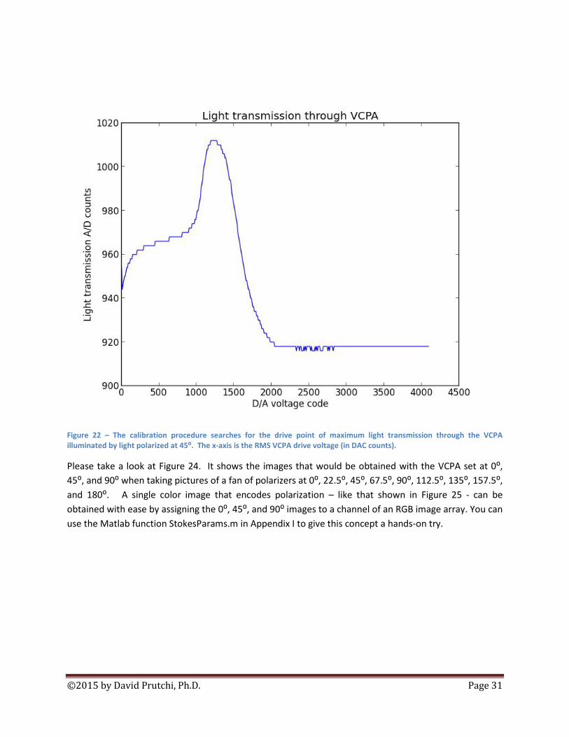
Figure 22 – The calibration procedure searches for the drive point of maximum light transmission through the VCPA illuminated by light polarized at 45⁰. The x-axis is the RMS VCPA drive voltage (in DAC counts).

Please take a look at Figure 24. It shows the images that would be obtained with the VCPA set at 0⁰, 45⁰, and 90⁰ when taking pictures of a fan of polarizers at 0⁰, 22.5⁰, 45⁰, 67.5⁰, 90⁰, 112.5⁰, 135⁰, 157.5⁰, and 180⁰. A single color image that encodes polarization – like that shown in Figure 25 - can be obtained with ease by assigning the 0⁰, 45⁰, and 90⁰ images to a channel of an RGB image array. You can use the Matlab function StokesParams.m in Appendix I to give this concept a hands-on try.


Figure 23 - A fan of linear polarizers oriented at 0⁰, 22.5⁰, 45⁰, 67.5⁰, 90⁰, 112.5⁰, 135⁰, 157.5⁰, and 180⁰ all look the same when observed through an unaided human eye. We wouldn’t even know there is something special about these rectangles if not for the arrows that I overlaid to explain the setup.

Figure 24 – I synthesized these grayscale test images using CorelDraw® to test DOLPi’s algorithms. The rectangles represent non-ideal polarizers at 0⁰, 22.5⁰, 45⁰, 67.5⁰, 90⁰, 112.5⁰, 135⁰, 157.5⁰, and 180⁰.


Figure 25 – A single color image that encodes polarization can be obtained with ease by combining the images acquired with the polarization analyzer set at 0⁰, 45⁰, and 90⁰ into an RGB image. This image was obtained by combining the sample images of Figure 24. Compare this figure to the unaided view of Figure 23 – The difference is dramatic to say the least!!!

Visualizing and Quantifying Polarization Assigning the images captured with the VCPA set at 0⁰, 45⁰, and 90⁰ to the RGB color channels is one simple way of visualizing polarization. However, the development of practical applications for this camera require some understanding of the way in which scientists and engineers describe the polarization of light under a more formal framework. Please keep on reading – I promise to keep this easy…

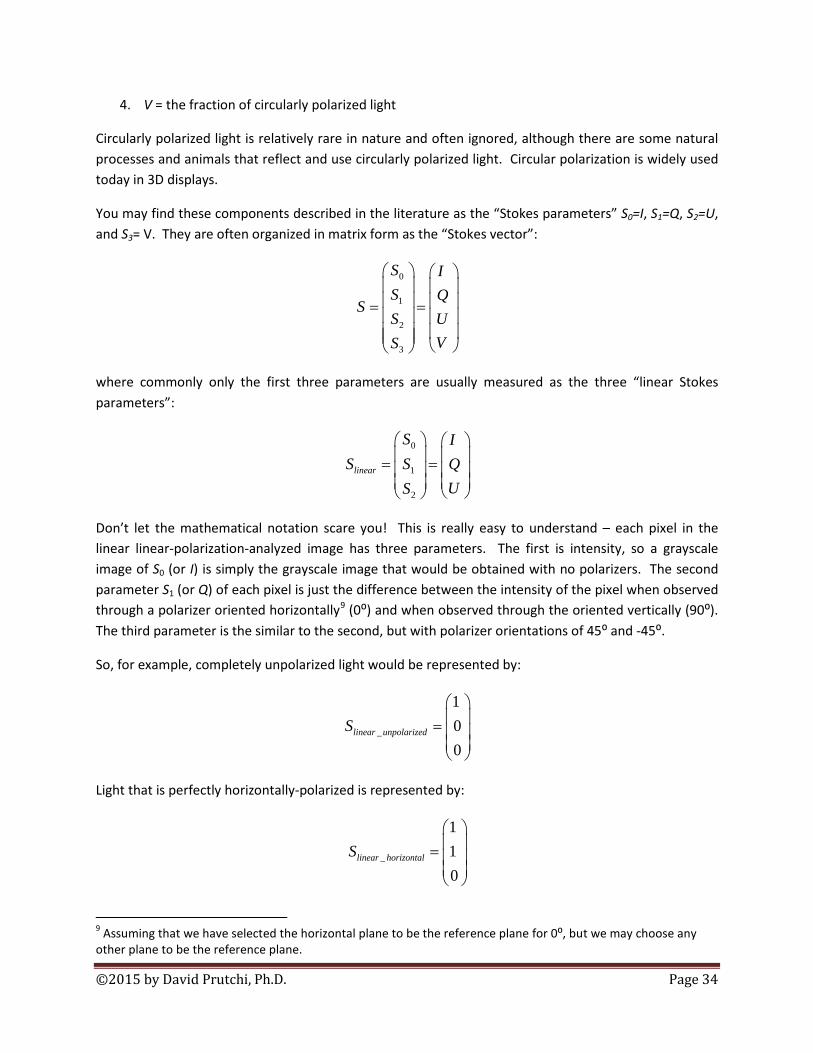
We must first understand that polarized light is seldom encountered in pure form. That is, objects in a scene rarely reflect light of perfectly polarized light. Instead, light is partially polarized to varying degrees because it contains components polarized in different directions. Four components are needed to completely describe light in terms of its polarization content. These are:

1. I = the overall intensity of the light 2. Q = the difference in intensity accepted through polarizers at 0⁰ and 90⁰ to the horizontal8 3. U = the difference in intensity accepted through polarizers at 45⁰ and -45⁰ to the horizontal

8 Using the horizontal plane as reference is one possible convention. However, a plane at any other angle may be used as the reference plane at 0⁰.


4. V = the fraction of circularly polarized light

Circularly polarized light is relatively rare in nature and often ignored, although there are some natural processes and animals that reflect and use circularly polarized light. Circular polarization is widely used today in 3D displays.

You may find these components described in the literature as the “Stokes parameters” S0=I, S1=Q, S2=U, and S3= V. They are often organized in matrix form as the “Stokes vector”:

0

1

2

3

S IS Q

SS U

VS

= =

where commonly only the first three parameters are usually measured as the three “linear Stokes parameters”:

0

1

2

linear

S IS S Q

US

= =

Don’t let the mathematical notation scare you! This is really easy to understand – each pixel in the linear linear-polarization-analyzed image has three parameters. The first is intensity, so a grayscale image of S0 (or I) is simply the grayscale image that would be obtained with no polarizers. The second parameter S1 (or Q) of each pixel is just the difference between the intensity of the pixel when observed through a polarizer oriented horizontally9 (0⁰) and when observed through the oriented vertically (90⁰). The third parameter is the similar to the second, but with polarizer orientations of 45⁰ and -45⁰.

So, for example, completely unpolarized light would be represented by:

_

100

linear unpolarizedS =

Light that is perfectly horizontally-polarized is represented by:

_

110

linear horizontalS =

9 Assuming that we have selected the horizontal plane to be the reference plane for 0⁰, but we may choose any other plane to be the reference plane.


Light that is perfectly vertically-polarized is represented by:

_

11

0linear horizontalS

= −

Light that is perfectly polarized at 45⁰ is represented by:

_

101

linear horizontalS =

And light that is perfectly polarized at 45⁰ is represented by:

_

10

1linear horizontalS

= −

For the sake of completeness, perfectly circularly-polarized light would be represented by the full Stokes vector as:

1 10 0

or 0 01 1

right hand left handS S− −

= =

−

DOLPi measures intensity at 0⁰, 45⁰, and 90⁰. Let’s call these I0⁰, I45⁰, and I90⁰, from which we need to calculate I, Q, and U. This would be straightforward if we would have a measurement at -45⁰ because the linear Stokes vector would be:

0 0 90

1 0 90

2 45 45

linear

S I IIS S Q I I

US I I

° °

° °

° − °

+ = = = −

−

However, the measurement at -45⁰ is not necessary, because it can be derived from the intensity of the other three angles, so all of the linear Stokes parameters can be calculated from I0⁰, I45⁰, and I90⁰:


0 0 90

1 0 90

2 45 0 902 linear

S I IIS S Q I I

US I I I

° °

° °

° ° °

+ = = = −

− −

Figure 26 – The Linear Stokes parameters calculated from the images of Figure 24. As the left image (S0=Intensity), the polarizers barely contrast with the background in my sample image.

The traditional way is to display polarization information as separate images for the intensity, degree of linear polarization, and the polarization angle. Strictly speaking, the Degree of Linear Polarization (DoLP) image is calculated for every pixel according to:

2 2

DoLPQ U

I+

=

While the Angle of Polarization (AoP) is calculated as:

1AoP arctan2

UQ

=

Overall intensity is typically displayed with a normal grayscale or color image of a scene, degree of polarization is displayed with a grayscale image of the same scene (black = 0% DoLP, white = 100% DoLP), and the angles of polarization are illustrated with different hues.


Figure 27 – The traditional way is to display polarization information as separate images for a) the Degree of Linear Polarization (DoLP), b) the angle of polarization (AoP), and c) the polarization intensity. These separate images are sometimes combined into a single color image using the Hue-Saturation-Intensity color model (d).

A popular way of presenting polarization information is by recognizing that the three main polarization components – polarization intensity, Degree of Linear Polarization, and Angle of Polarization - are analogous to the color components of brightness, saturation, and hue. The polarization parameters merged into the HSV (Hue, Saturation, Value) color space is shown in Figure 28.

In the HSV color model, as hue varies from 0 to 1, the corresponding colors vary from red through yellow, green, cyan, blue, magenta, and back to red, so that there are actually red values both at 0 and 1. To represent AoP, a hue value of 0 is assigned to 0⁰, while a hue value of 1 is assigned to 180⁰.

Saturation is assigned to the Degree of Linear Polarization. As DoLP varies from 0 to 1, the corresponding colors (hues) vary from unsaturated (shades of gray) to fully saturated (no white component).

Lastly, value (brightness) is assigned to Polarization Intensity. As it varies from 0 to 1.0, the corresponding colors become increasingly brighter.


Figure 28 – HSV representation of polarization parameters (DoLP, AoP, and Polarization Intensity) for the images of Figure 24. The figure at the right is the colormap for the HSV image.

It is interesting to compare the image produced by a simple RGB merge of the individual grayscale images acquired by setting the analyzer at 0⁰, 45⁰, and 90⁰ (Figure 29-a) with that obtained from combining the calculated DoLP, AoP, and Polarization Intensity images through the HSV model (Figure 29-b). The HSV model provides better contrast and more quantifiable information about a scene’s polarization. However, the calculation of intermediate parameters takes processing time, so the simple RGB merge is often a good tradeoff as a preview for the sake of attaining a higher frame rate.

Figure 29 – A simple RGB merge of the grayscale images obtained at polarization analyzer settings of 0⁰, 45⁰, and 90⁰ (a) suffices as a real-time preview of the HSV representation (b) obtained through more complex calculation of DoLP, AoP, and Polarization Intensity from the linear Stokes parameters.

I hope that this section didn’t give you a headache! Although the math is relatively simple, you can now appreciate that it is difficult for us to intuitively integrate the sense of light polarization into the way we normally use our vision (that is, through the analysis of intensity and color). I believe that this unintuitive nature of polarization has been responsible for slowing down the development of practical


applications for polarimetric imaging. I encourage you to review this section once again so that you can understand what is it that we are viewing when looking at a polarization image.

Polarized Light in the Environment Non-polarized light becomes polarized when it is reflected by a nonmetallic surface. The degree of polarization depends on the angle at which the light hits the surface, as well as on the type of reflective material. As shown in Figure 30, water, snow fields, and asphalt roads reflect the Sun’s light with very strong horizontal polarization (i.e. parallel to the reflective surface).

The glare produced by these reflections can be diminished through the use of vertically-polarized sunglasses. Next time you go to a fishpond, pay attention how much easier it is to see fish when your sunglasses are in their “normal” position (the orientation of their polarizers being vertical) versus when you tilt your head sideways and thus align your sunglasses’ polarization with that of the water’s surface.

Many aquatic insects use their polarization-sensitive vision to locate ponds. For example, insects that lay eggs in water find and select egg-laying sites based on the intensity of polarization from reflective water surfaces. Unfortunately, many human-made objects can reflect horizontally polarized light so strongly that they appear to aquatic insects to be bodies of water. Some – like solar panels – reflect light with such high level of horizontal polarization (close to 100%) that they look to aquatic insects as far superior breeding grounds than pond water (which reflects light with a degree of polarization of around 30 to 70%), becoming ecological death traps to these organisms [Horvath et al, 2010].


Figure 30 – Non-polarized light becomes polarized when it is reflected by a nonmetallic surface. The degree of polarization depends on the angle at which the light hits the surface, as well as on the type of reflective material. Water, snow fields, and asphalt roads reflect the Sun’s light with very strong horizontal polarization. Vertically-polarized sunglasses thus cut the glare produced by horizontally-polarized reflections.

Another natural source of polarized light is scattering of sunlight in the atmosphere. The exact mechanism is outside the scope of this article, but suffice it to say that sunlight that is scattered backwards (or forward) by the atmosphere remains unpolarized, while light scattered at 90⁰ degrees from the Sun’s position becomes linearly polarized, while light scattered at intermediate angles is only partially polarized (Figure 31). If you are interested in more detail, Glenn S. Smith from Georgia Tech published an excellent, easy-to-understand paper with college-level math that really explains the process of sunlight polarization by atmospheric scattering [Smith, 2007].

As shown in Figure 25, the polarization vectors in the sky are all oriented along parallel circles centered on the Sun's position. Being able to see the distribution of polarization angles can be used as an orientation cue. In fact, sky polarization patterns are used by many insects for navigation. For example, honeybees use celestial polarization to move between the hive and foraging locations. Salmons are thought to have similar capabilities to orient themselves based on the sky’s polarization as seen underwater.

It is hypothesized that the Vikings knew how to navigate this way based on a legend that tells of a glowing “sunstone” that, when held up to the sky, revealed the position of the Sun even on a cloudy day. This would have been important since constant daylight during the summer sailing season at high latitudes would have prevented them from using the stars as a guide to their positions. Even a magnetic compass, which is believed to have been unknown to the Vikings, would have been almost useless so close to the magnetic North Pole. The theory thus goes that a natural polarizing crystal such as calcite


would have helped the Vikings find the position of the Sun even through thick fog and overcast skies [Horváth, 2011].

Figure 31 – The sky is polarized tangential to a circle centered on the Sun. A band of maximum polarization occurs 90⁰ from the Sun. At sunrise and sunset, the sky is maximally polarized along the meridian, and thus vertically-polarized at the horizon. On the other hand, at noon the band of maximum polarization is horizontally polarized along the horizon. Many insects use sky polarization patterns for navigation. Honeybees use celestial polarization to move between the hive and foraging locations.

So… What about the Cloaked UFOs? I have never seen a UFO, and don’t know anyone who claims to have seen one either. In addition, I am not aware of any compelling evidence that we are being visited by extraterrestrial beings, so I remain skeptical. However, it is fun to imagine how massive alien (or military) craft could be made to fly in our skies without being seen. Maybe the craft could be rendered transparent? Maybe it could bend or reflect the light around it so that it is cloaked within a bubble of invisibility? Maybe it could use an active cloaking screen that paints an image of the background on its surface?

We don’t have to go extraterrestrial to find examples of these cloaking methods. Just go into the ocean and you’ll find dozens of species that camouflage themselves through transparency and mirror reflection. However, these cloaking strategies can be defeated by animals that have evolved polarization-sensitive vision, and the same could possibly work against artificial cloaking devices. As a matter of fact, polarization cues are so important underwater that evolution has given some animals – like cuttlefish (Figure 32) – polarization-sensitive instead of color-sensitive vision [Les, 2012].


Figure 32 – Cuttlefish are color-blind, but have polarization-sensitive vision with a resolution of about 1⁰. They are often referred to as the "chameleons of the sea" because of their remarkable ability to rapidly alter their skin color and pattern - including polarization - to camouflage themselves, to scare potential predators, and to communicate to other cuttlefish. "Cuttlefish @ Oceanário de Lisboa" by David Sim via Wikimedia Commons.

Transparent animals are never completely transparent, but their refraction index is sufficiently well matched to that of water that it is difficult to see from a distance. However, transparent tissues modify the polarization of light, either by increasing or decreasing its polarization state, such that they will contrast against their background when seen through polarization-sensitive eyes. For example, polarization-sensitive squid can detect zooplankton prey at 70% greater distance under partially polarized lighting than under nonpolarized lighting

In the same way, cancerous cells reflect and scatter light with different polarization characteristics than those of healthy cells. Just as with color, polarization differences can provide additional contrast cues to detect malignant cells. This technique is being investigated by a number of researchers [Antonelli et al., 2009], and I believe that DOLPi could enable the development of a cheap and effective “smart mirror” for at-home skin cancer screening.

Polarimetric imaging is an excellent contrast-enhancing technique because its information supplements the knowledge that can be derived from intensity and color imaging. Spectral characteristics (color) depend largely on the materials that make up the objects in a scene. However, the polarization properties depend strongly on the microscopic shape of a reflective surface (roughness) and its orientation. As such, spectral and polarization information supplement each other by contributing independent features for the detection and characterization of camouflaged objects or those hidden in a cluttered environment. Furthermore, man-made objects often reflect light with some degree of polarization when they incorporate non-metallic surfaces such as glass, plastic, paints, and rubbers. Since most natural backgrounds do not polarize light, man-made materials are highlighted by color in


DOLPi images. Neither camouflage nor moderate foliage escape a polarimetric imager, making it possible to develop new methods for humanitarian detection and clearance of land mines [El-Saba et al, 2008].

Polarimetric imaging with DOLPi can thus be used for a large number of image enhancement tasks such as glare reduction, haze removal, background removal, and contrast enhancement. These are highly valuable for forensic work, industrial and environmental monitoring, microscopic investigation of tissues and plastics, and autonomous vehicle vision just to name a few.

The Need for Speed The single largest shortcoming with DOLPi in its current incarnation is its slow frame rate. This is caused by the long time that it takes picamera to perform a single-shot frame capture. There are some tricks that I still have to try10, but we’ll probably have to wait for faster GPU firmware that will enable frame capture rates to produce smooth video even in preview mode.

The Raspberry Pi camera is able to acquire a set of frames quite quickly, so I tried using the camera’s STROBE and FREX signals11 to synchronize frame acquisition with changes in the VCPA’s state. Unfortunately, activating these hardware signals needs to be done from the Raspberry Pi’s GPU, which has closed-source firmware. I am not aware of anyone finding yet a hack to enable STROBE and FREX.

Low frame rates may not be a problem at all when imaging processes that change very slowly. DOLPi’s frame rates more than suffice for capturing polarization images for medical diagnostics, atmospheric pollution monitoring, and scanning for hidden targets in a static scene.

However, some of the most promising applications of polarimetric imaging are contrast-enhancing techniques that enable the same type of feats performed by animals with polarization-sensitive vision (e.g. navigation, camouflage breaking, object recognition, etc.). To make these useful – such as for underwater vision by autonomous submarines (AUVs), the polarimetric imaging system needs to be fast to allow real-time use by machine-vision algorithms.

Instead of trying to change the polarization state of an analyzer placed in front of a sensor, high-speed polarization imagers have been built using multiple sensors, each with its dedicated, fixed-state polarization analyzer. The simplest type consists of two imaging sensors placed behind orthogonal polarizing filters. As shown in Figure 33-a, this can be accomplished by placing two CCD cameras behind the output ports of a polarizing beamsplitter cube.

As shown in Figure 33-b, to acquire the complete linear Stokes parameter vector, a 3-way beamsplitting prism can be used to send copies of the scene to three CCD camera sensors, each placed behind a polarizer. This is the approach taken by FluxData for its FD-1665 polarization camera

10 For example, using a generator function within capture_sequence for changing the state of the VCPA as described in http://raspberrypi.stackexchange.com/questions/22040/take-images-in-a-short-time-using-the-raspberry-pi-camera-module. 11 These lines are available in the Raspberr Pi camera clone made by Arducam (Rev.C OV5647).


(http://www.fluxdata.com/imaging-polarimeters). I have been working on a DIY version of this camera by replacing the color filters of a 3-CCD color camera by polarization filters. My results so far are not very good, mostly due to the difficulty of taking apart the beamsplitter prism. I am currently building my own 3-way splitter and polarization filters to convert a 3-CCD JVC KY-F55BU color camera into an imaging polarimeter. In fact, I have been thinking about going retro all the way, and hacking a 3-tube (vidicon) color camera to make it easier to disassemble or replace the 3-way beamsplitter12. The advantage of starting from a 3-CCD (or 3-vidicon) camera is that the mechanical alignment hardware, as well as the image-combining circuitry is already built. Here it is worthwhile mentioning a Matlab-driven polarimetric camera of this kind built by Mark Umansky for his M.Sc. thesis using multiple, synchronized machine-vision cameras viewing the scene through a DIY beamsplitter assembly.

Lately, CCD imaging sensors have been fitted with micropolarizer arrays with linear polarizers (Figure 33-c) – much in the same way that color CCD image sensors are fitted with a color filter array. The pixelated polarization camera can then acquire multiple polarization orientations in a single video frame, enabling instantaneous measurements of the linear Stokes parameters. This is probably beyond a DIY project, so we’ll have to wait for one of the commercial outfits to mass-produce a low-cost CCD with integrated polarization filter array. Hopefully, DOLPi will muster enough attention for this to happen. If you really need this type of performance for your project right away, you could contact Moxtek (http://moxtek.com/optics-product/pixelated-polarizer/) or 4D Technologies (http://www.4dtechnology.com/products/polarcam.php).

12 http://blog.robindeits.com/2014/02/07/driving-a-viewfinder-from-1982/ describes the teardown of a vintage 3-tube JVC color camera. It looks like a promising model to modify into a polarimetric imager.

http://www.fluxdata.com/imaging-polarimeters

http://moxtek.com/optics-product/pixelated-polarizer/

http://www.4dtechnology.com/products/polarcam.php

http://blog.robindeits.com/2014/02/07/driving-a-viewfinder-from-1982/


Figure 33 – Polarization imaging frame rate can be increased by using multiple sensors, each dedicated to a single angle of polarization analysis and then combining these into a single image through high-speed processing circuitry. a) In its simplest form, a measurement of two orthogonal polarizations can be used to calculate the first two Stokes parameters, which may suffice for many applications. b) The complete linear Stokes parameter vector can be obtained by routing copies of the scene to three separate image sensors via polarizing filters set at 0⁰, 45⁰, and 90⁰. c) Another possibility is to filter the individual pixels of an imaging sensor – much like it’s done in a color camera, but using polarizing filters instead of the usual color filter array.

Saving the World DOLPi will be there to save the day if Wonder Woman ever turns into a supervillain bent on destroying the world with her transparent jet. Barring that scenario, DOLPi will probably serve more as a low-cost foundation for the development of applications based on polarization-sensitive imaging and machine vision. However, the disruptive power of this technology is truly awesome!

The use of polarimetric imaging for skin cancer detection was discussed above. Developing a low-cost self-examination camera to screen for skin cancers would have an enormous impact on world health. Just consider that according to the American Academy of Dermatology, one in five Americans will develop skin cancer in the course of a lifetime! A screening technique based on DOLPi would


dramatically change the effect of this disease since basal cell and squamous cell carcinomas, the two most common forms of skin cancer, are highly curable if detected early and treated properly.

Besides direct healthcare, polarimetric imaging has started to be used for satellite-based characterization of atmospheric aerosol particles – a worldwide problem of significant impact. In fact, particle size, chemical composition, and shape can only be measured by including polarization information into a satellite’s imaging capabilities [Snik et al., 2014]. Unfortunately, satellite observations only show what can be seen from above, and not what hides below layers of clouds and pollution.

DOLPi opens up the field of polarimetric imaging to the citizen scientist, enabling the development of techniques for remote sensing of vast swaths of atmosphere [Kreuter et al., 2013] to detect and characterize pollution and volcanic ash, giving the public unfiltered access to information about the nature and sources of hazardous air contaminants.

DOLPi also enables the development of low-cost tools for real-time monitoring of volcanic emissions, providing advanced data to populations at risk, as well as to local airports and air traffic such that appropriate warnings can be issued to those in harm’s way.

Lastly, and with a more strategic view, DOLPi gives researchers and enthusiast scientists the possibility of developing networks of low-cost sensors to measure atmospheric aerosol scattering and absorption properties that at are presently the principal source of uncertainty in climate modeling.

It is my hope that DOLPi will introduce fellow hackers and engineers to the awesome power of polarimetric imaging and inspire the development of breakthrough applications ranging from environmental monitoring and medical diagnostics, to security and antiterrorism applications.

References

Antonelli MR, Pierangelo A, Novikova T, DeMartino A, “Polarimetric Imaging of Human Tissue for Cancer Diagnostics: Experiment and Monte Carlo Modeling”, http://www.biop.dk/biophotonics09/Poster/Antonelli_NewSummary.pdf, 2009.

Bushman BB, Object Detector, U.S. Patent 5,404,225, Apr. 4, 1995.

deJong W, Schavemaker J, “Using Polarization Features of Visible Light for Automatic Landmine Detection” in Physics of Automatic Target Recognition - Advanced Sciences and Technologies for Security Applications, 3, 73-90, 2007.

El-Saba A, Bezuayehu T, "Higher Probability of Detection of Subsurface Land Mines with a Single Sensor using Multiple Polarized and Unpolarized Image Fusion”, in Polarization: Measurement, Analysis, and Remote Sensing VIII, edited by Chenault, David B.; Goldstein, Dennis H., Proceedings of the SPIE, 6972, 2008.

http://www.biop.dk/biophotonics09/Poster/Antonelli_NewSummary.pdf


Horváth G, Blahó M, Egri A, Kriska G, Seres I, Robertson B, “Reducing the Maladaptive Attractiveness of Solar Panels to Polarotactic Insects”, Conservation Biology, 24(6), 1644-1653, 2010.

Horváth G, Barta A, Pomozi I, Suhai B, Hegedüs R, Åkesson S, Meyer-Rochow B, Wehner R, “On the Trail of Vikings with Polarized Skylight: Experimental Study of the Atmospheric Optical Prerequisites Allowing Polarimetric Navigation by Viking Seafarers”, Phil. Trans. R. Soc. B, 366, 772–782, 2011.

Kreuter A, Blumthaler M, “Feasibility of Polarized All-Sky Imaging for Aerosol Characterization”, Atmos. Meas. Tech., 6, 1845–1854, 2013

Lefaudeux N, Method and System for Stokes Polarization Imaging, U.S. Patent 8,004,675, Aug. 23, 2011.

Les C.B., “Polarization Vision Keeps Cuttlefish Safe”, Photonics Showcase, 7, July 2012.

Prutchi D, Prutchi SR, Exploring Quantum Physics through Hands-On Projects, 335 pages, John Wiley & Sons, Inc., Hoboken, NJ, 2012.

Smith GS, “The Polarization of Skylight: An Example from Nature”, American Journal of Physics, 75(1), 25-31, 2007.

Snik F, Craven-Jones J, Escuti M, Fineschi S, Harrington D, de Martino S, Mawet D, Riedih J, Tyo JS, “An Overview of Polarimetric Sensing Techniques and Technology with Applications to Different Research Fields”, Conclusions from an Interactive, Multidisciplinary Workshop on Polarimetric Techniques and Technology at the Lorentz Center in Leiden, the Netherlands, March 24-28, 2014.

Umansky M, A Prototype Polarimetric Camera for Unmanned Ground Vehicles, M.Sc. Thesis, Virginia Polytechnic Institute and State University, 2013.

Vedel M, Breugnota S, LechocinskiaN, “Full Stokes Polarization Camera”, SPIE Proc. Vol. 8160-33, SPIE Optical Engineering + Applications, San Diego, Aug 21-25, 2011

Appendix I – StokesParams.m - Matlab Function for Calculating and Displaying Stokes and Polarization Parameter Images function StokesParameters = StokesParams (I90, I45, I0, option) % Function StokesParams.m % Calculates and displays Stokes and polarization parameter images % ---------------------------------------------------------------- % % Inputs: % Im90, Im45, Im0, Option % where: % Im0 = Image at 90 degrees % Im45 = Image at 45 degrees % Im0 = Image at 0 degrees % Option = 1 or 2 % where: % Option = 1: Internally converts color RGB image to grayscale


% Option = 2: Uses grayscale (UINT8) image arrays % % Calculates and displays Stokes parameter images % ----------------------------------------------- % S0 = I % S1 = Q % S2 = U % % Calculates and displays polarization images % ------------------------------------------- % Pol_int = Polarization Intensity % Pol_deg = Degree of Linear Polarization (DoLP) % Pol_angle = Angle of Polarization (AoP) % Ih, Iv if option ==1 % Convert RGB images to grayscale double I90 = rgb2gray(im2double(I90)); I0 = rgb2gray(im2double(I0)); I45 = rgb2gray(im2double(I45)); elseif option ==2 % Convert UINT8 grayscale images to double I90 = im2double(I90); I45 = im2double(I45); I0 = im2double(I0); end % Calculate Stokes parameters, I, Q, U (S0 S1 S2) % I = I0 + I90 % Q = I0 - I90 % U = 2I45 - I0 - I90 StokesParameters.I = I0 + I90 ; StokesParameters.Q = I0 - I90 ; StokesParameters.U = 2.*I45 - I0 - I90 ; % Polarization intensity = sqrt (Q^2 + U^2) StokesParameters.Pol_int = sqrt(StokesParameters.Q.^2 + StokesParameters.U.^2) ; % Degree of Linear Polarization = Polarization intensity / I StokesParameters.DoP = StokesParameters.Pol_int./StokesParameters.I ; % Angle of Polarization = 0.5 * atan(U/Q) StokesParameters.Pol_ang = 0.5.* atan2(StokesParameters.U,StokesParameters.Q); % Polarization ratio = Q/I StokesParameters.Pol_ratio = StokesParameters.Q./StokesParameters.I ; % Ih = 0.5(I+Q) StokesParameters.Ih = 0.5.*(StokesParameters.I+StokesParameters.Q) ; % Iv = 0.5(I-Q) StokesParameters.Iv = 0.5.*(StokesParameters.I-StokesParameters.Q) ; % Display source images and combine into RGB representation figure; subplot(2,2,1); imshow(I90); title('Red = Analyzer polarization: 90 degrees'); subplot (2,2,2);


imshow(I0); title('Green = Analyzer polarization: 0 degrees') subplot(2,2,3) imshow(I45); title('Blue = Analyzer polarization: 45 degrees') subplot(2,2,4); RGBpol(:,:,1)=I90; RGBpol(:,:,2)=I0; RGBpol(:,:,3)=I45; imshow(RGBpol) title('RGB Representation of Polarization') axis('off') %figure %imshow(RGBpol) %title('RGB Representation of Polarization') %axis('off') % Display Stokes parameter images figure subplot(2,2,1) imagesc(StokesParameters.I,[0,1]) title('I (Stokes S0)'); colormap('jet') colorbar axis('off') subplot(2,2,2) imagesc(StokesParameters.Q,[0,1]) title('Q (Stokes S1)'); colormap('jet') colorbar axis('off') subplot(2,2,3) imshow(StokesParameters.U,[0,1]) title('U (Stokes S2)'); colormap('jet') colorbar axis('off') % Display polarization parameter images figure; imagesc(StokesParameters.Pol_int) colormap('jet') title('Polarization Intensity') colorbar axis('off') figure imagesc(StokesParameters.DoP,[0,1]) colormap('gray') title('Degree of Linear Polarization (DOLP)') colorbar axis('off') figure imagesc(StokesParameters.Pol_ratio)


colormap('gray') title('Polarization Ratio'); axis('off') figure imagesc((StokesParameters.Pol_ang+(pi/2))*(180/pi),[0,180]) colormap('hsv') title('Angle of Polarization (AoP)') colorbar axis('off') figure; subplot(1,2,1) imagesc(StokesParameters.Ih) colormap('jet') colorbar axis('off') title('Ih') subplot(1,2,2) imagesc(StokesParameters.Iv); colormap('jet') colorbar title('Iv') axis('off') % Display HSV components and representation figure HSV(:,:,1)=(StokesParameters.Pol_ang+(pi/2))/pi; HSV(:,:,2)=StokesParameters.DoP; HSV(:,:,3)=StokesParameters.Pol_int; subplot(2,2,1) imagesc(HSV(:,:,1),[0,1]) title('H = Angle of Polarization (AoP)') colormap('jet'); axis('off') subplot(2,2,2) imagesc(HSV(:,:,2),[0,1]) colormap('jet'); axis('off') title('S = Degree of Linear Polarization (DoLP)') subplot(2,2,3) imagesc(HSV(:,:,3),[0,1]) title('V = Polarization Intensity') colormap('jet'); axis('off') subplot(2,2,4) imshow(hsv2rgb(HSV)) axis('off') title('Polarization (HSV Representation)') % Display HSV representation along colormap of HSV space figure subplot(1,2,1) imshow(hsv2rgb(HSV)) axis('off') title('Polarization (HSV Representation)') subplot(1,2,2) % Show color cone imshow(imread('HSV_color_map.jpg'));

DOLPi – A Low-Cost, RasPi-based Polarization Camera

Documents

Transcript of DOLPi – A Low-Cost, RasPi-based Polarization Camera