

Doing more with less: economically-efficient management of ...Doing more with less:...
81
Doing more with less: economically-efficient management of pavement networks Jeremy Gregory ACPA Mid-Year Meeting June 13, 2017
Transcript of Doing more with less: economically-efficient management of ...Doing more with less:...
Doing more with less:
economically-efficient management
of pavement networks
Jeremy Gregory
ACPA Mid-Year Meeting
June 13, 2017
Slide 2
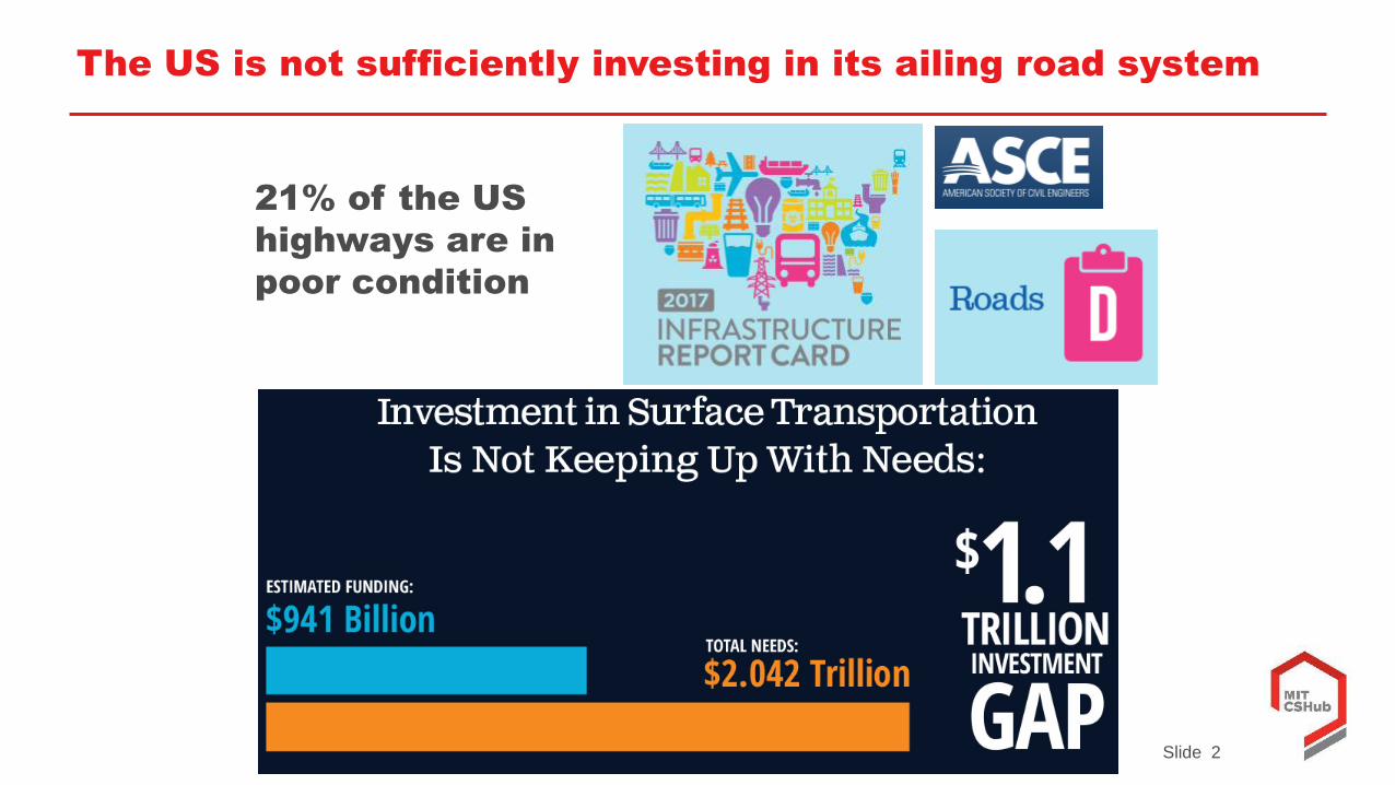
The US is not sufficiently investing in its ailing road system
21% of the US
highways are in
poor condition
Slide 3
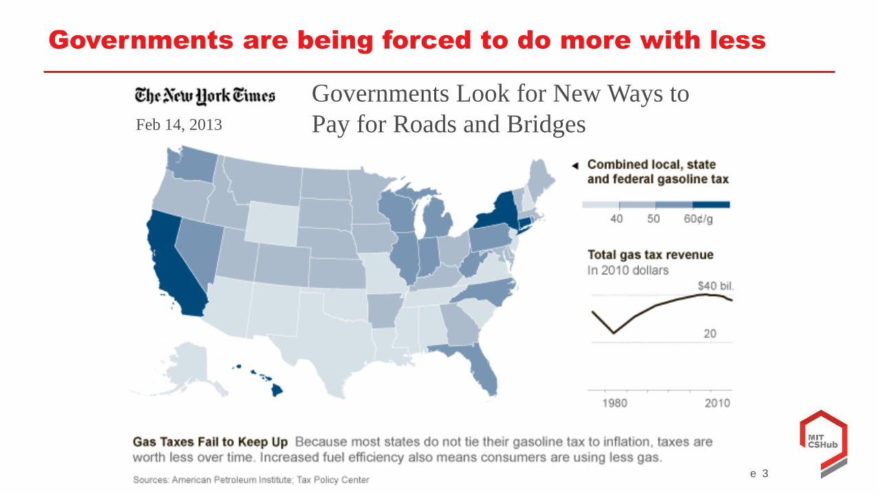
Governments are being forced to do more with less
Governments Look for New Ways to
Pay for Roads and BridgesFeb 14, 2013
Slide 4
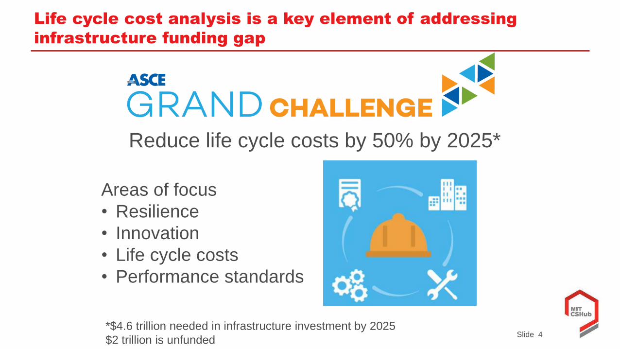
Life cycle cost analysis is a key element of addressing
infrastructure funding gap
Reduce life cycle costs by 50% by 2025*
Areas of focus
• Resilience
• Innovation
• Life cycle costs
• Performance standards
*$4.6 trillion needed in infrastructure investment by 2025
$2 trillion is unfunded
Slide 5
Asset management allocation tools are critical to
economically-efficient infrastructure
Use asset management best practices to prioritize projects
and improve the condition, security, and safety of assets
while minimizing costs over its entire life span.
Slide 6
Tools for economically-efficient management of pavement
networks
Competitive Paving Prices
Life Cycle Cost Analysis
Asset Management
Slide 7
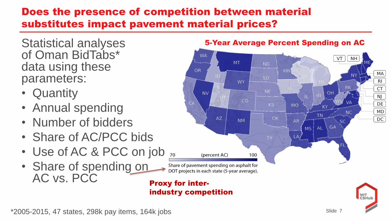
Statistical analysesof Oman BidTabs* data using these parameters:
• Quantity
• Annual spending
• Number of bidders
• Share of AC/PCC bids
• Use of AC & PCC on job
• Share of spending on AC vs. PCC
5-Year Average Percent Spending on AC
Proxy for inter-
industry competition
Does the presence of competition between material
substitutes impact pavement material prices?
*2005-2015, 47 states, 298k pay items, 164k jobs
Slide 8
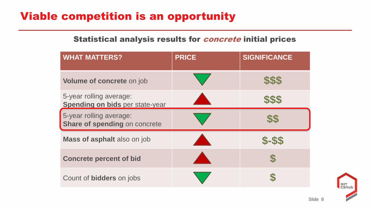
Viable competition is an opportunity
WHAT MATTERS? PRICE SIGNIFICANCE
Volume of concrete on job
5-year rolling average:
Spending on bids per state-year
5-year rolling average:
Share of spending on concrete
Mass of asphalt also on job
Concrete percent of bid
Count of bidders on jobs
Statistical analysis results for concrete initial prices
$$$
$$$
$$
$-$$
$
$
Slide 9
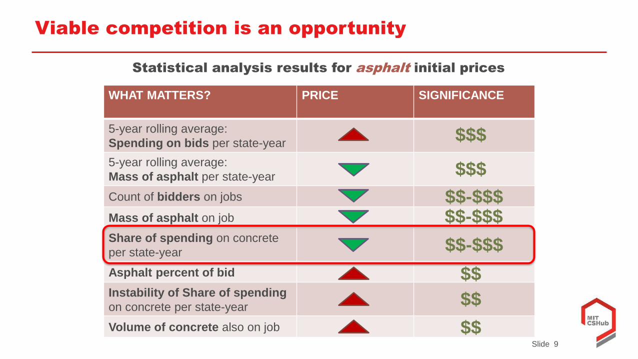
Viable competition is an opportunity
WHAT MATTERS? PRICE SIGNIFICANCE
5-year rolling average:
Spending on bids per state-year
5-year rolling average:
Mass of asphalt per state-year
Count of bidders on jobs
Mass of asphalt on job
Share of spending on concrete
per state-year
Asphalt percent of bid
Instability of Share of spending
on concrete per state-year
Volume of concrete also on job
Statistical analysis results for asphalt initial prices
$$$
$$$
$$
$$
$$-$$$$$-$$$
$$-$$$
$$

Slide 10
Tools for economically-efficient management of pavement
networks
Competitive Paving Prices
Life Cycle Cost Analysis
Asset Management
Slide 11
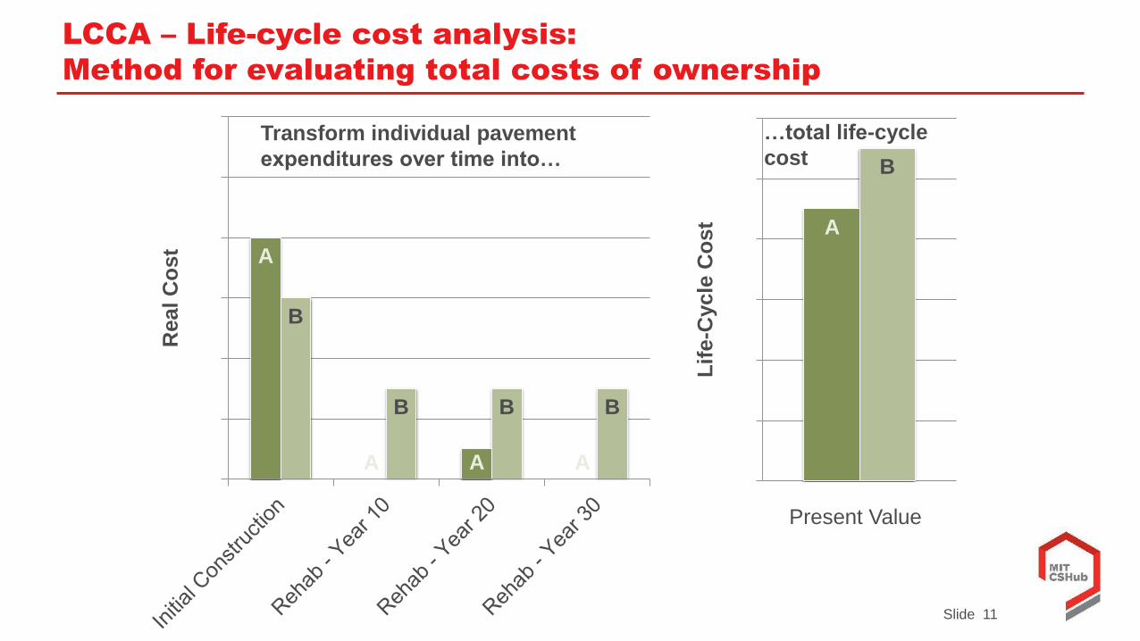
LCCA – Life-cycle cost analysis:
Method for evaluating total costs of ownership
A
A A A
B
B B B
0
2
4
6
8
10
12
Real C
ost
A
B
0
2
4
6
8
10
12
Lif
e-C
ycle
Co
st
Transform individual pavement
expenditures over time into…
…total life-cycle
cost
Present Value
Slide 12
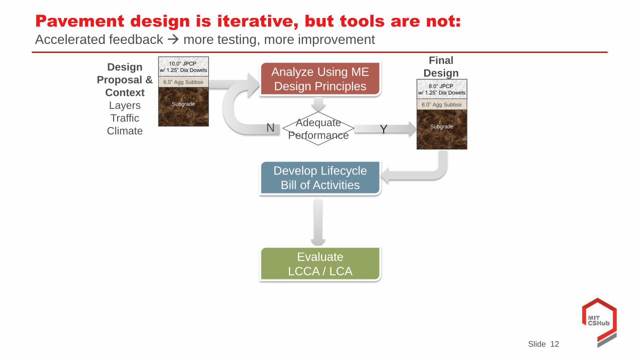
Pavement design is iterative, but tools are not:
Accelerated feedback more testing, more improvement
10.0” JPCP
w/ 1.25” Dia Dowels
Subgrade
6.0” Agg Subbse
Design
Proposal &
Context
Layers
Traffic
Climate
Analyze Using ME
Design Principles
N Adequate
Performance
8.0” JPCP
w/ 1.25” Dia Dowels
Subgrade
6.0” Agg Subbse
Final
Design
Develop Lifecycle
Bill of Activities
Evaluate
LCCA / LCA
Y
Slide 13
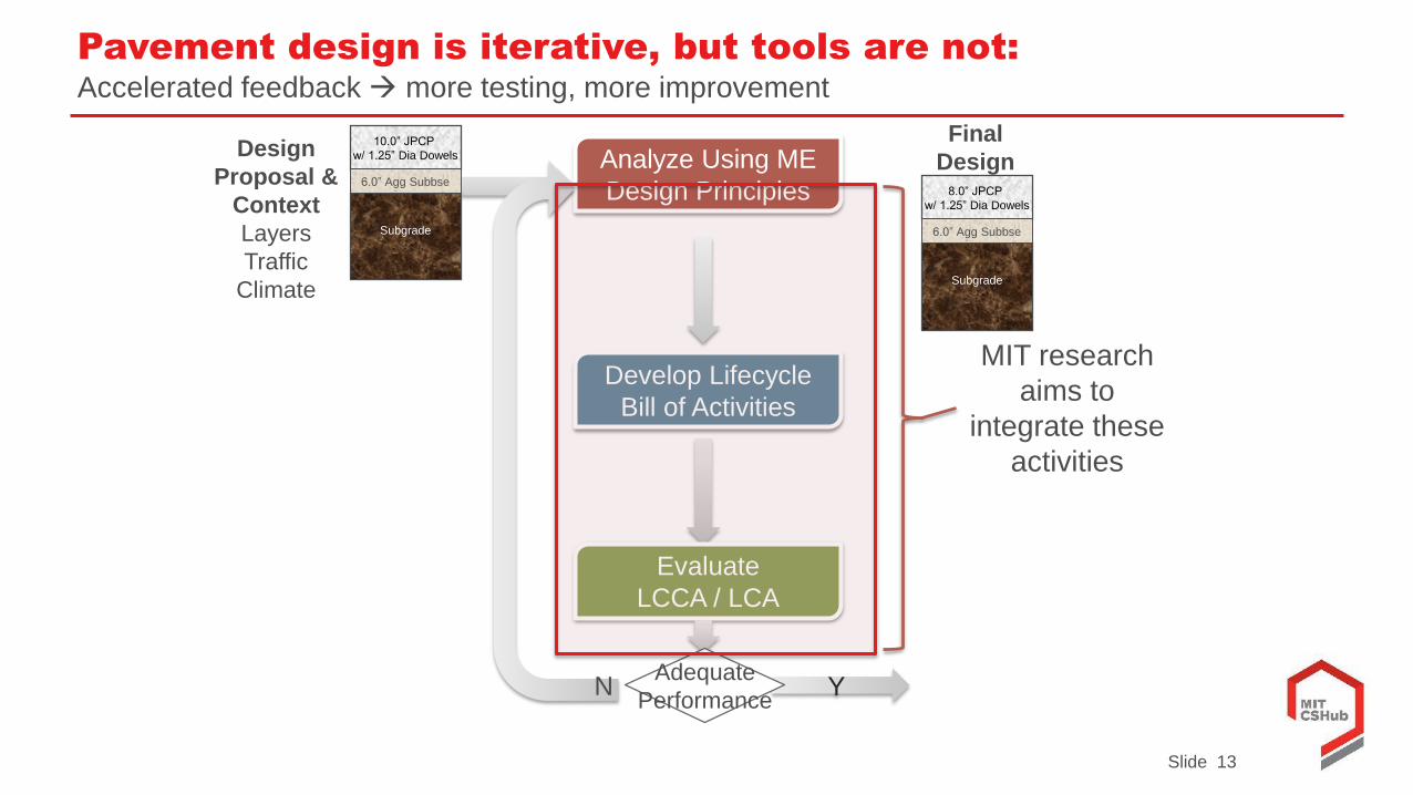
Pavement design is iterative, but tools are not:
Accelerated feedback more testing, more improvement
10.0” JPCP
w/ 1.25” Dia Dowels
Subgrade
6.0” Agg Subbse
Design
Proposal &
Context
Layers
Traffic
Climate
Analyze Using ME
Design Principles
Develop Lifecycle
Bill of Activities
Evaluate
LCCA / LCA
N YAdequate
Performance
MIT research
aims to
integrate these
activities
8.0” JPCP
w/ 1.25” Dia Dowels
Subgrade
6.0” Agg Subbse
Final
Design
Slide 14
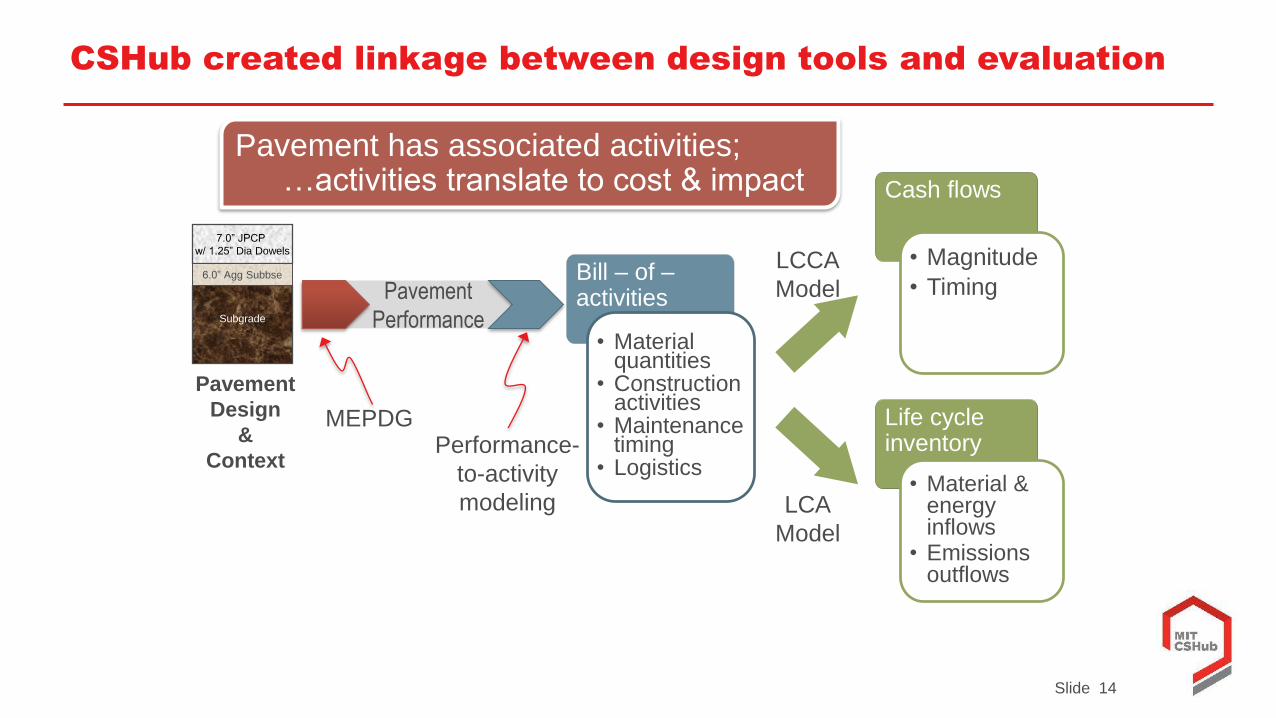
CSHub created linkage between design tools and evaluation
Life cycle inventory
• Material & energy inflows
• Emissions outflows
Bill – of –activities
• Material quantities
• Construction activities
• Maintenance timing
• Logistics
Cash flows
• Magnitude
• Timing
7.0” JPCP
w/ 1.25” Dia Dowels
Subgrade
6.0” Agg Subbse
Pavement
Design
&
Context
MEPDG
LCCA
Model
LCA
Model
Pavement
Performance
Performance-
to-activity
modeling
Pavement has associated activities;…activities translate to cost & impact
Slide 15
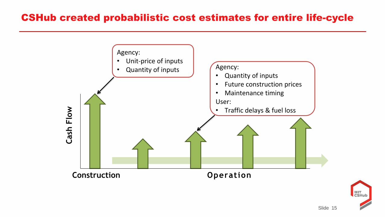
CSHub created probabilistic cost estimates for entire life-cycle
Construction Operation
Cash
Flo
w
Agency:• Unit-price of inputs• Quantity of inputs Agency:
• Quantity of inputs• Future construction prices• Maintenance timingUser:• Traffic delays & fuel loss
Slide 16
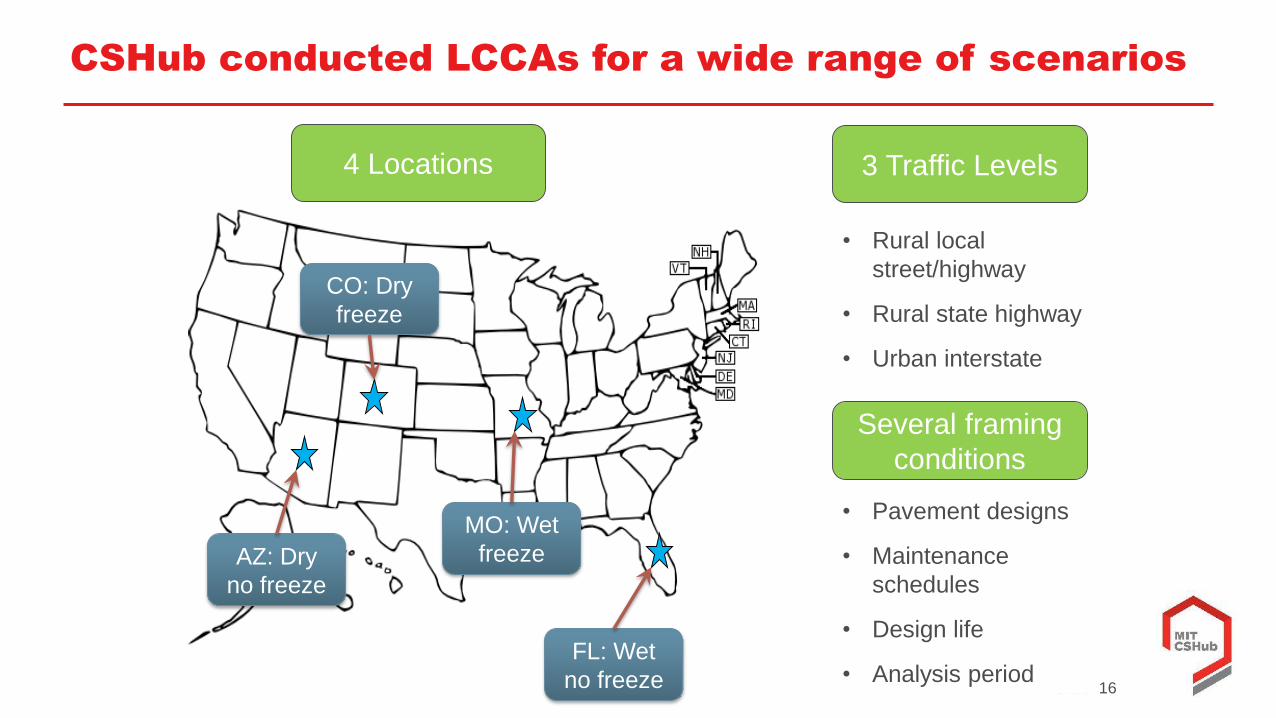
CSHub conducted LCCAs for a wide range of scenarios
4 Locations
FL: Wet
no freeze
MO: Wet
freeze
CO: Dry
freeze
AZ: Dry
no freeze
3 Traffic Levels
• Rural local
street/highway
• Rural state highway
• Urban interstate
Several framing
conditions
• Pavement designs
• Maintenance
schedules
• Design life
• Analysis period
Slide 17
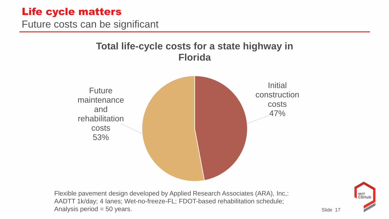
Life cycle matters
Future costs can be significant
Initial construction
costs47%
Future maintenance
and rehabilitation
costs53%
Total life-cycle costs for a state highway in Florida
Flexible pavement design developed by Applied Research Associates (ARA), Inc,:
AADTT 1k/day; 4 lanes; Wet-no-freeze-FL; FDOT-based rehabilitation schedule;
Analysis period = 50 years.
Slide 18
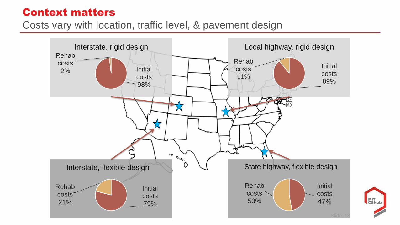
Context matters
Costs vary with location, traffic level, & pavement design
Initial costs98%
Rehab costs2%
Interstate, rigid design
Initial costs79%
Rehab costs21%
Interstate, flexible design
Initial costs47%
Rehab costs53%
State highway, flexible design
Initial costs89%
Rehab costs11%
Local highway, rigid design
Slide 19
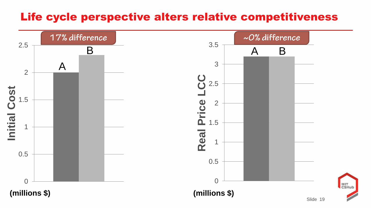
Life cycle perspective alters relative competitiveness
0
0.5
1
1.5
2
2.5
Init
ial
Co
st
A
B
0
0.5
1
1.5
2
2.5
3
3.5
Re
al
Pri
ce
LC
C
A B
(millions $) (millions $)
Slide 20
0%
25%
50%
75%
100%
2.00 2.50 3.00 3.50 4.00
Fre
qu
en
cy
Net Present Value of LCC (million $)
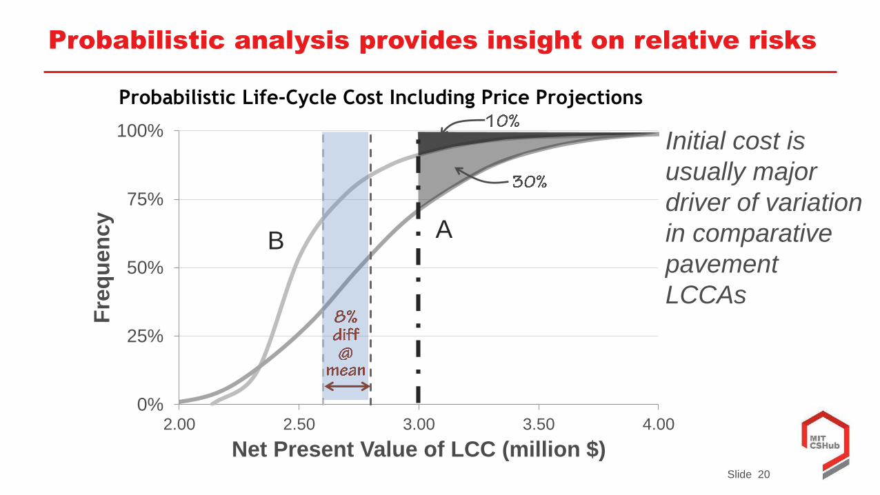
Probabilistic analysis provides insight on relative risks
Probabilistic Life-Cycle Cost Including Price Projections
B A
Initial cost is
usually major
driver of variation
in comparative
pavement
LCCAs
Slide 21
Tools for economically-efficient management of pavement
networks
Competitive Paving Prices
Life Cycle Cost Analysis
Asset Management
Slide 22
FHWA has issued new performance management rules due to
MAP-21
FHWA motivation for
performance management:
• Provide the most efficient investment of Federal
transportation funds
• Refocus on national transportation goals
• Increase accountability and transparency
• Improve decision-making through performance-
based planning and programming
Slide 23
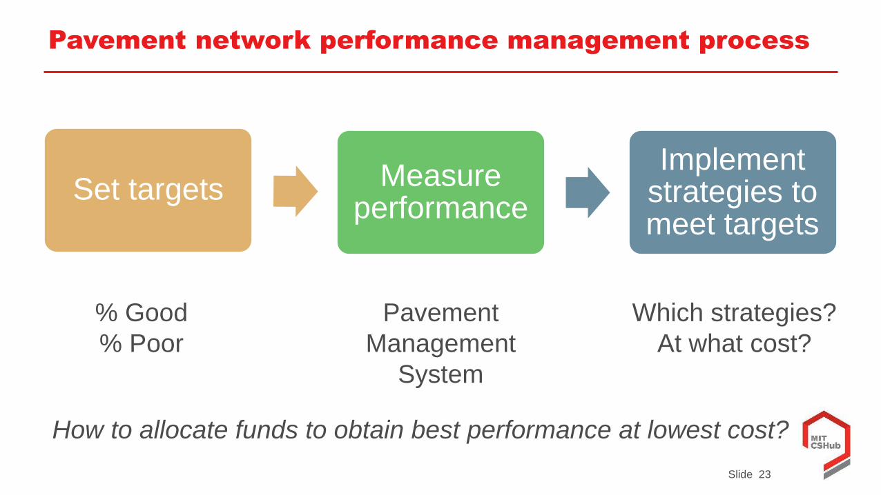
Pavement network performance management process
Set targets Measure performance
Implement strategies to meet targets
% Good
% Poor
Pavement
Management
System
Which strategies?
At what cost?
How to allocate funds to obtain best performance at lowest cost?
Slide 24
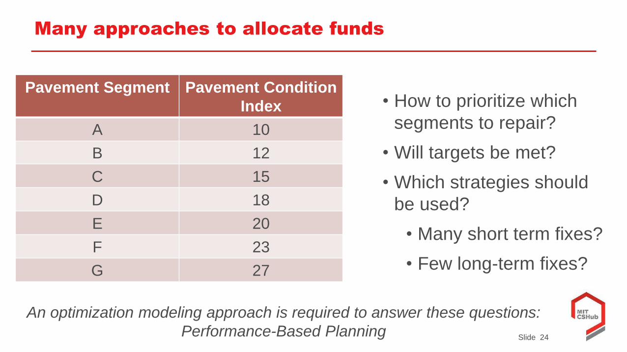
Many approaches to allocate funds
Pavement Segment Pavement Condition
Index
A 10
B 12
C 15
D 18
E 20
F 23
G 27
• How to prioritize which
segments to repair?
• Will targets be met?
• Which strategies should
be used?
• Many short term fixes?
• Few long-term fixes?
An optimization modeling approach is required to answer these questions:
Performance-Based Planning
Slide 25
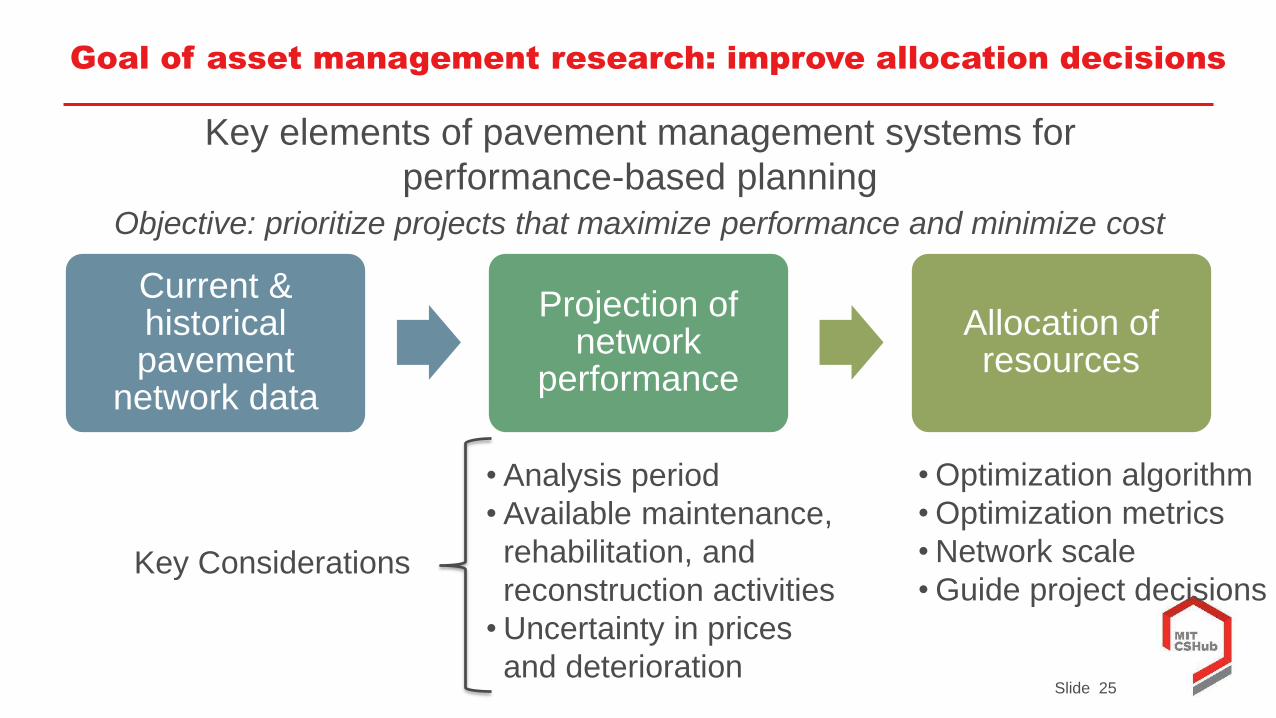
Goal of asset management research: improve allocation decisions
Current & historical pavement
network data
Projection of network
performance
Allocation of resources
Key elements of pavement management systems for
performance-based planning
Objective: prioritize projects that maximize performance and minimize cost
• Analysis period
• Available maintenance,
rehabilitation, and
reconstruction activities
• Uncertainty in prices
and deterioration
• Optimization algorithm
• Optimization metrics
• Network scale
• Guide project decisionsKey Considerations
Slide 26
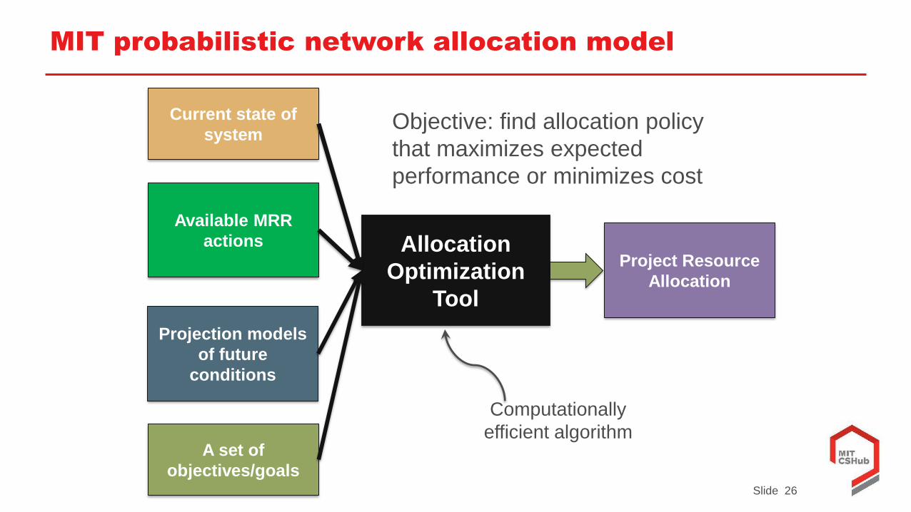
MIT probabilistic network allocation model
Allocation
Optimization
Tool
Current state of
system
Projection models
of future
conditions
A set of
objectives/goals
Available MRR
actions
Objective: find allocation policy
that maximizes expected
performance or minimizes cost
Project Resource
Allocation
Computationally
efficient algorithm
Slide 27
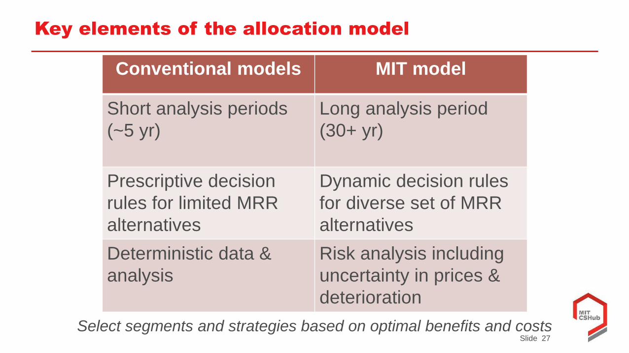
Key elements of the allocation model
Conventional models MIT model
Short analysis periods
(~5 yr)
Long analysis period
(30+ yr)
Prescriptive decision
rules for limited MRR
alternatives
Dynamic decision rules
for diverse set of MRR
alternatives
Deterministic data &
analysis
Risk analysis including
uncertainty in prices &
deterioration
Select segments and strategies based on optimal benefits and costs
Slide 28
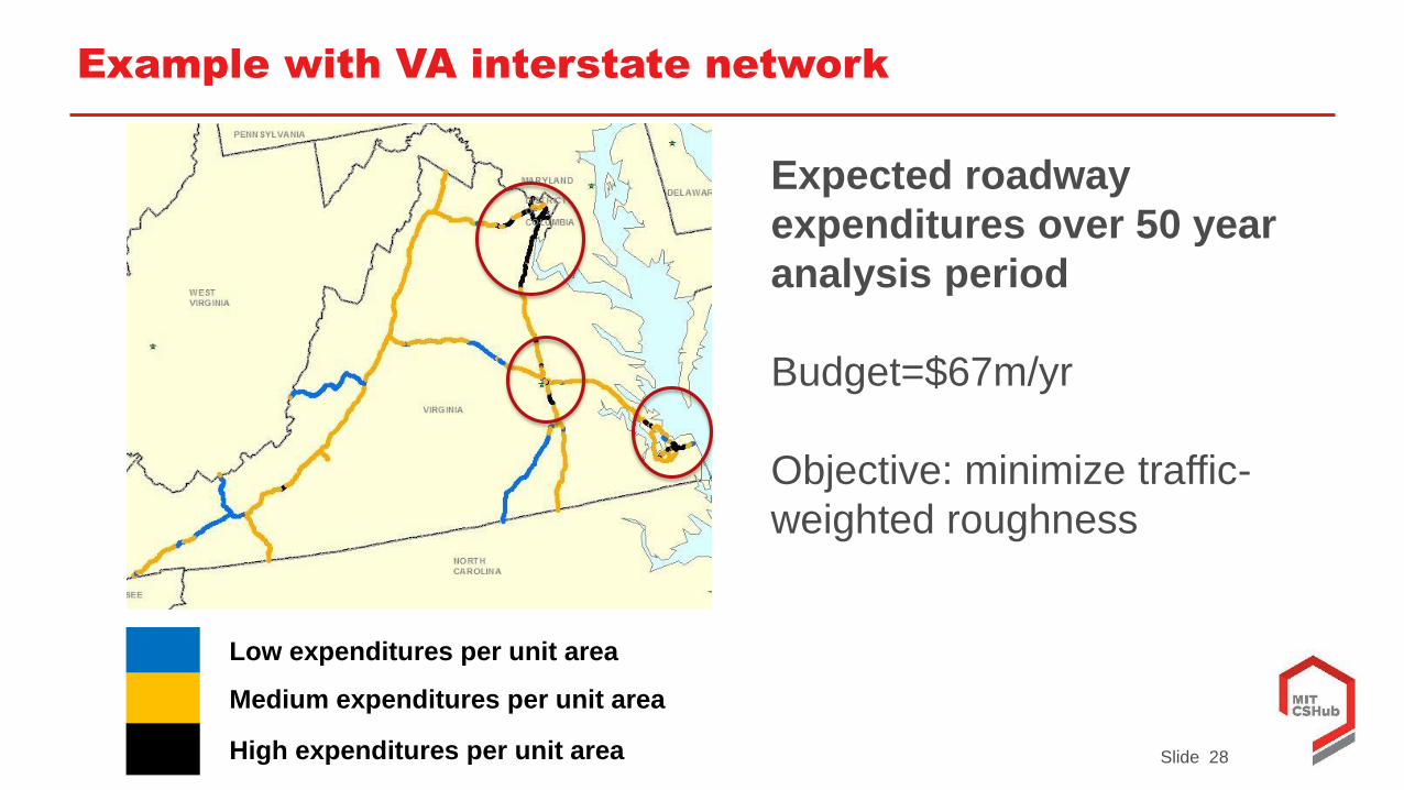
Example with VA interstate network
Low expenditures per unit area
Medium expenditures per unit area
High expenditures per unit area
Expected roadway
expenditures over 50 year
analysis period
Budget=$67m/yr
Objective: minimize traffic-
weighted roughness
Slide 29
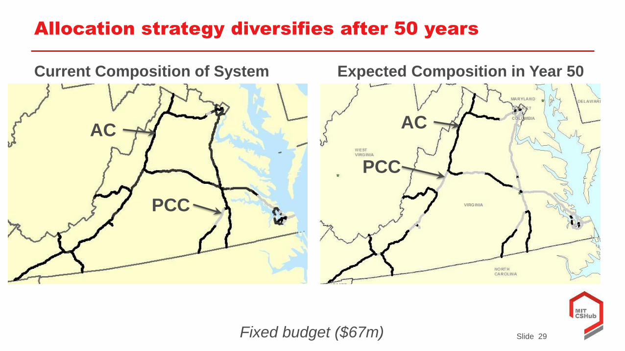
Allocation strategy diversifies after 50 years
Current Composition of System Expected Composition in Year 50
AC
PCC
Fixed budget ($67m)
AC
PCC
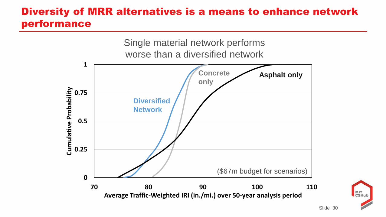
Slide 30
Diversity of MRR alternatives is a means to enhance network
performance
0
0.25
0.5
0.75
1
70 80 90 100 110
Cu
mu
lati
ve P
rob
abili
ty
Average Traffic-Weighted IRI (in./mi.) over 50-year analysis period
Diversified
Network
Concrete
onlyAsphalt only
($67m budget for scenarios)
Single material network performs
worse than a diversified network
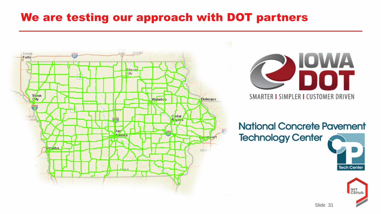
Slide 31
We are testing our approach with DOT partners

Slide 33
LIFE-CYCLE COST:
Details on the CSHub Approach
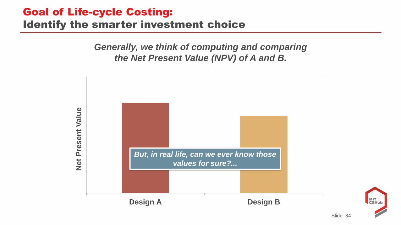
Slide 34
Design A Design B
Net
Pre
sen
t V
alu
e
Generally, we think of computing and comparing
the Net Present Value (NPV) of A and B.
Goal of Life-cycle Costing:
Identify the smarter investment choice
But, in real life, can we ever know those
values for sure?...
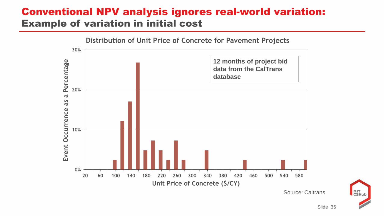
Slide 35
Conventional NPV analysis ignores real-world variation:
Example of variation in initial cost
0%
10%
20%
30%
20 60 100 140 180 220 260 300 340 380 420 460 500 540 580
Event
Occurr
ence a
s a P
erc
enta
ge
Unit Price of Concrete ($/CY)
Distribution of Unit Price of Concrete for Pavement Projects
Source: Caltrans
12 months of project bid
data from the CalTrans
database
Slide 36
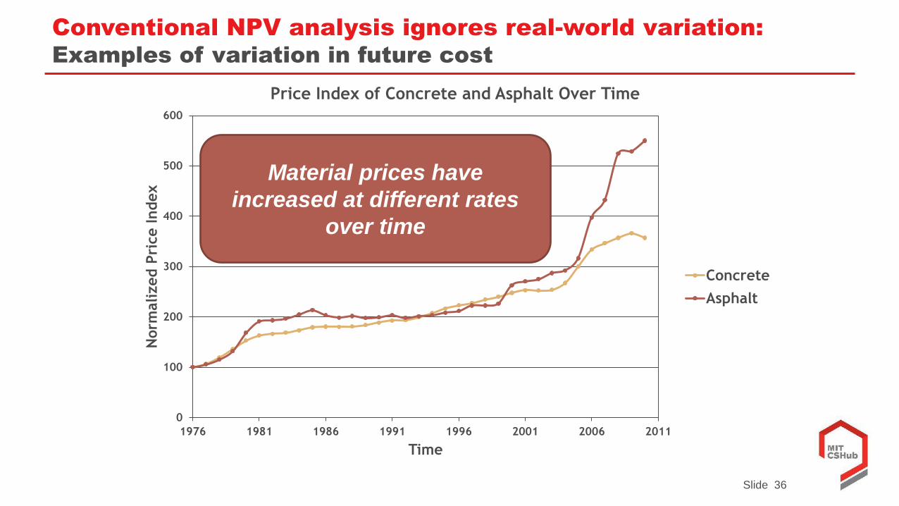
Conventional NPV analysis ignores real-world variation:
Examples of variation in future cost
0
100
200
300
400
500
600
1976 1981 1986 1991 1996 2001 2006 2011
Norm
alized P
rice Index
Time
Price Index of Concrete and Asphalt Over Time
Concrete
Asphalt
Material prices have
increased at different rates
over time
Slide 37
0
40
80
120
160
1975 1980 1985 1990 1995 2000 2005 2010 2015
Norm
alized R
eal Pri
ce Index
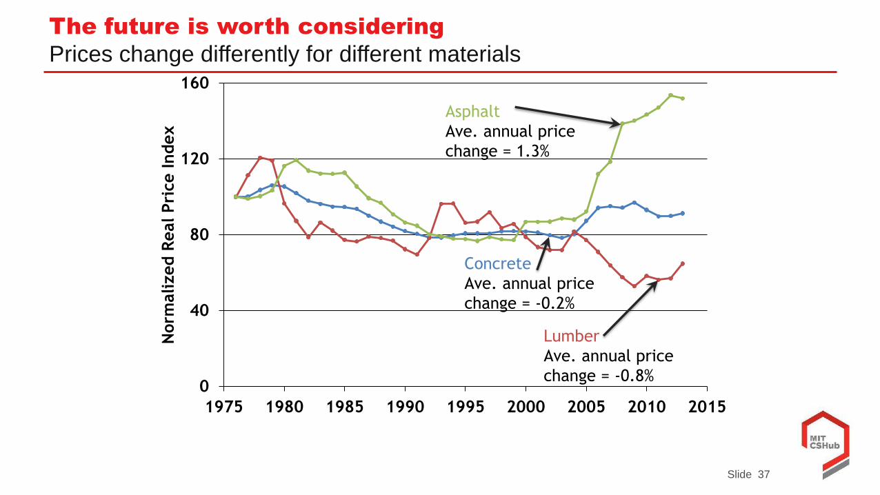
Asphalt
Ave. annual price
change = 1.3%
Concrete
Ave. annual price
change = -0.2%
Lumber
Ave. annual price
change = -0.8%
The future is worth considering
Prices change differently for different materials
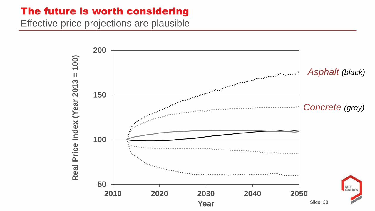
Slide 38
The future is worth considering
Effective price projections are plausible
Concrete (grey)
Asphalt (black)
50
100
150
200
2010 2020 2030 2040 2050
Re
al P
ric
e In
de
x (
Ye
ar
20
13
= 1
00
)
Year
Slide 39
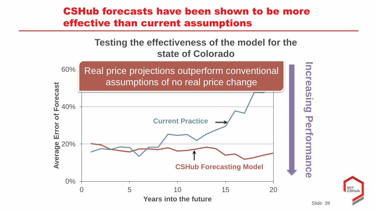
CSHub forecasts have been shown to be more
effective than current assumptions
0%
20%
40%
60%
0 5 10 15 20
Av
era
ge E
rro
r o
f F
ore
cast
Years into the future
CSHub Forecasting Model
Current Practice
Incre
asin
g P
erfo
rman
ce
Testing the effectiveness of the model for the
state of Colorado
Real price projections outperform conventional
assumptions of no real price change
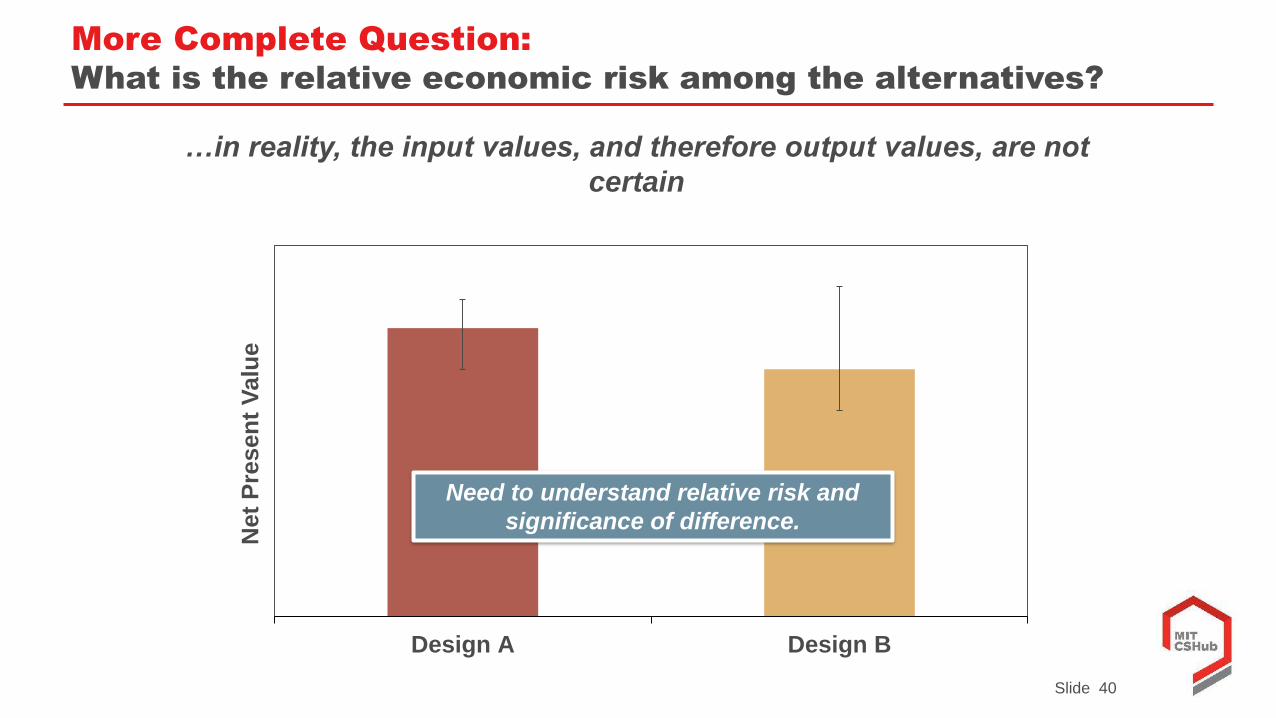
Slide 40
Design A Design B
Net
Pre
sen
t V
alu
e
…in reality, the input values, and therefore output values, are not
certain
More Complete Question:
What is the relative economic risk among the alternatives?
Need to understand relative risk and
significance of difference.
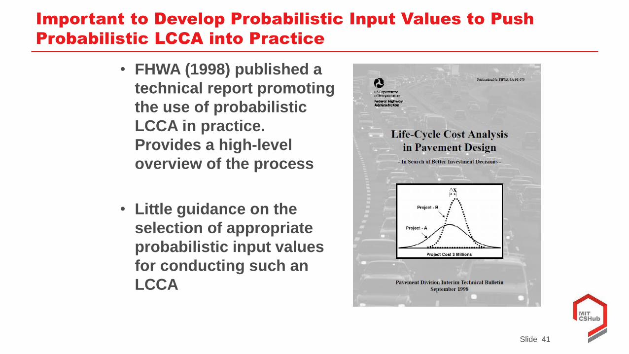
Slide 41
Important to Develop Probabilistic Input Values to Push
Probabilistic LCCA into Practice
• FHWA (1998) published a
technical report promoting
the use of probabilistic
LCCA in practice.
Provides a high-level
overview of the process
• Little guidance on the
selection of appropriate
probabilistic input values
for conducting such an
LCCA
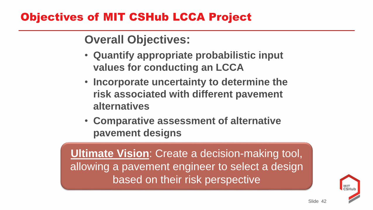
Slide 42
Objectives of MIT CSHub LCCA Project
Overall Objectives:
• Quantify appropriate probabilistic input
values for conducting an LCCA
• Incorporate uncertainty to determine the
risk associated with different pavement
alternatives
• Comparative assessment of alternative
pavement designs
Ultimate Vision: Create a decision-making tool,
allowing a pavement engineer to select a design
based on their risk perspective
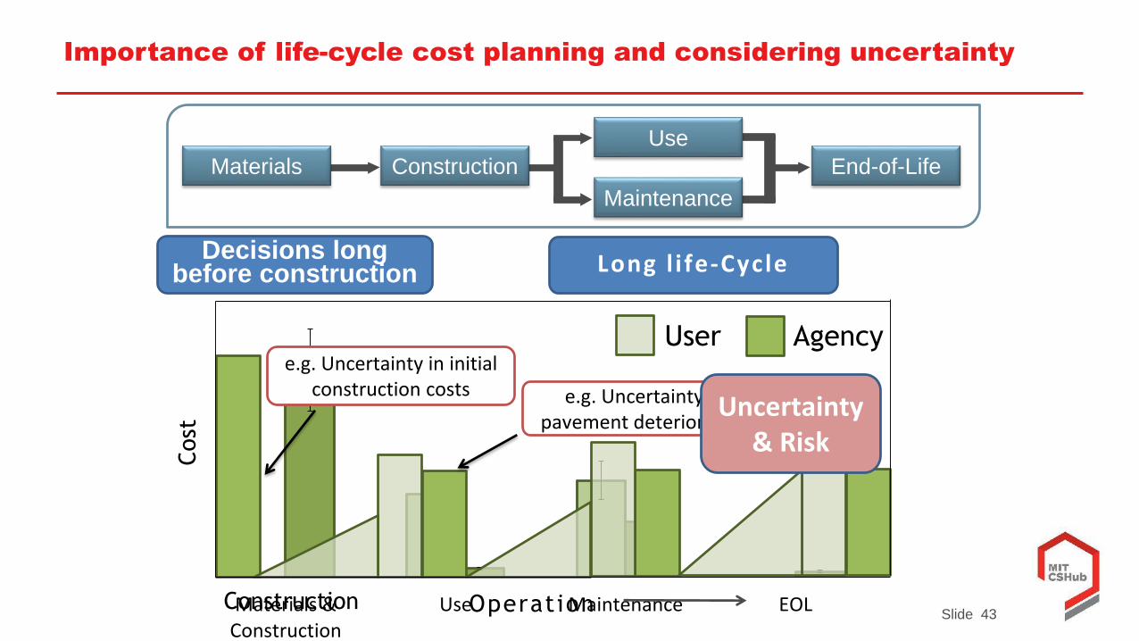
Slide 43Materials &
ConstructionUse Maintenance EOL
User Agency
Importance of life-cycle cost planning and considering uncertainty
Construction Operation
CostMaterials End-of-LifeConstruction
Use
Maintenance
Long l i fe-CycleDecisions long before construction
e.g. Uncertainty in initial construction costs e.g. Uncertainty in
pavement deteriorationUncertainty
& Risk
Slide 44
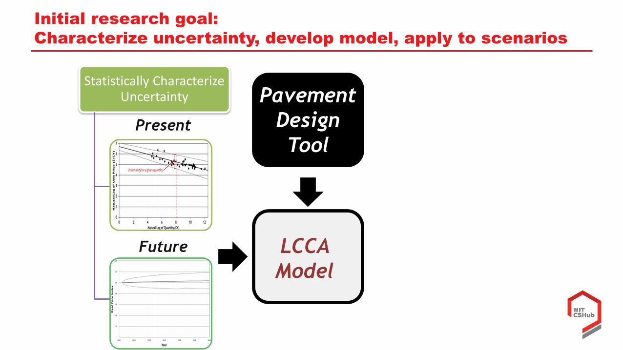
Initial research goal:
Characterize uncertainty, develop model, apply to scenarios
Statistically Characterize Uncertainty
Propagate uncertainty to understand risk
LCCA
Model
Pavement
Design
ToolPresent
Future
Is the difference
significant?
Relative risk
Characterize drivers of
uncertainty
Slide 45
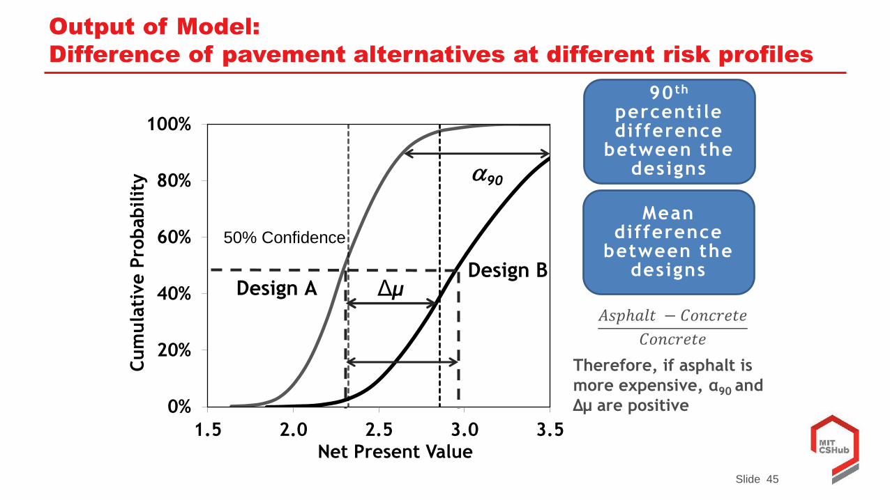
Output of Model:
Difference of pavement alternatives at different risk profiles
0%
20%
40%
60%
80%
100%
1.5 2.0 2.5 3.0 3.5
Cum
ula
tive P
robabilit
y
Net Present Value
Design BDesign A
Mean difference
between the designs
90 th
percentile difference
between the designs
𝐴𝑠𝑝ℎ𝑎𝑙𝑡 − 𝐶𝑜𝑛𝑐𝑟𝑒𝑡𝑒
𝐶𝑜𝑛𝑐𝑟𝑒𝑡𝑒
Therefore, if asphalt is
more expensive, α90 and
Δμ are positive
Δμ
a90
50% Confidence
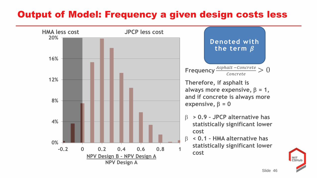
Slide 46
Output of Model: Frequency a given design costs less
Denoted with the term 𝛽
Frequency𝐴𝑠𝑝ℎ𝑎𝑙𝑡 −𝐶𝑜𝑛𝑐𝑟𝑒𝑡𝑒
𝐶𝑜𝑛𝑐𝑟𝑒𝑡𝑒> 0
Therefore, if asphalt is
always more expensive, b = 1,
and if concrete is always more
expensive, b = 0
0%
4%
8%
12%
16%
20%
-0.2 0 0.2 0.4 0.6 0.8 1
NPV Design B – NPV Design ANPV Design A
JPCP less costHMA less cost
b > 0.9 – JPCP alternative has
statistically significant lower
cost
b < 0.1 – HMA alternative has
statistically significant lower
cost
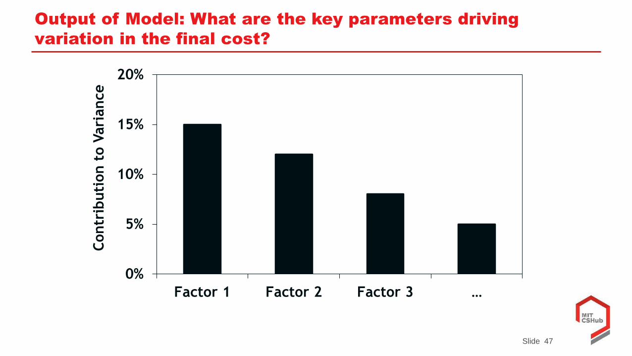
Slide 47
Output of Model: What are the key parameters driving
variation in the final cost?
0%
5%
10%
15%
20%
Factor 1 Factor 2 Factor 3 …
Contr
ibuti
on t
o V
ari
ance
Slide 48
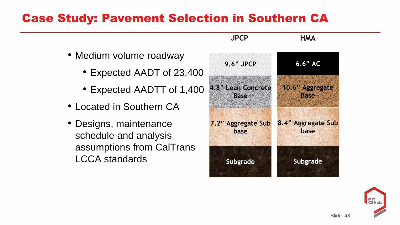
Case Study: Pavement Selection in Southern CA
• Medium volume roadway
• Expected AADT of 23,400
• Expected AADTT of 1,400
• Located in Southern CA
• Designs, maintenance
schedule and analysis
assumptions from CalTrans
LCCA standards
HMAJPCP
Subgrade
8.4” Aggregate Sub
base
10.6” Aggregate
Base
6.6” AC
Subgrade
7.2” Aggregate Sub
base
4.8” Lean Concrete
Base
9.6” JPCP
Slide 49
Case Study: Three types of analyses conducted
Three types of analyses are conducted:
1) Initial Costs (no uncertainty)
2)Real price adjusted life cycle cost (no uncertainty)
3)Full probabilistic life-cycle cost (with uncertainty)
The purpose is to understand:
a) The impact of scope of analysis
b) The impact of risk on the decision
Slide 50
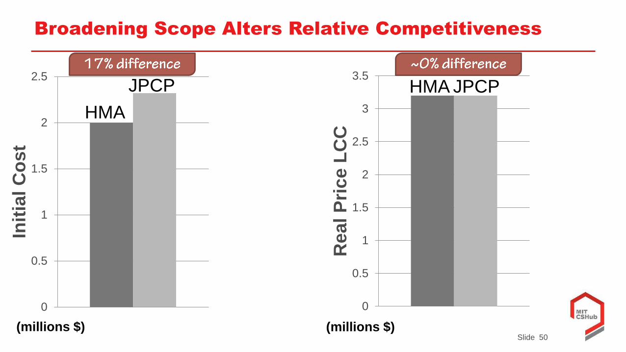
Broadening Scope Alters Relative Competitiveness
0
0.5
1
1.5
2
2.5
Init
ial
Co
st
HMA
JPCP
0
0.5
1
1.5
2
2.5
3
3.5
Re
al
Pri
ce
LC
C
HMA JPCP
(millions $) (millions $)
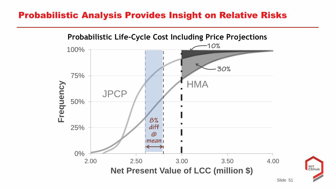
Slide 51
0%
25%
50%
75%
100%
2.00 2.50 3.00 3.50 4.00
Fre
qu
en
cy
Net Present Value of LCC (million $)
Probabilistic Analysis Provides Insight on Relative Risks
Probabilistic Life-Cycle Cost Including Price Projections
JPCPHMA
Slide 52
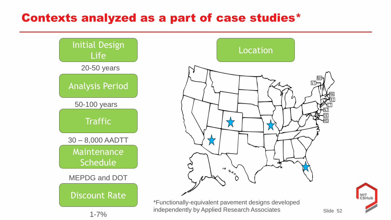
Contexts analyzed as a part of case studies*
Traffic
Initial Design
Life
Analysis Period
Location
Maintenance
Schedule
20-50 years
50-100 years
30 – 8,000 AADTT
MEPDG and DOT
Discount Rate
1-7%
*Functionally-equivalent pavement designs developed
independently by Applied Research Associates
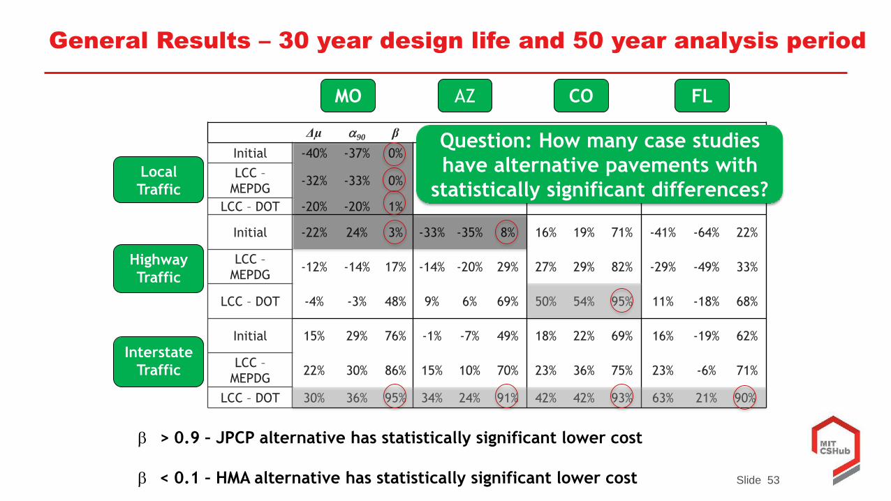
Slide 53
General Results – 30 year design life and 50 year analysis period
Δµ a90 β Δµ a90 β Δµ a90 β Δµ a90 β
Initial -40% -37% 0%
LCC –
MEPDG-32% -33% 0%
LCC – DOT -20% -20% 1%
Initial -22% 24% 3% -33% -35% 8% 16% 19% 71% -41% -64% 22%
LCC –
MEPDG-12% -14% 17% -14% -20% 29% 27% 29% 82% -29% -49% 33%
LCC – DOT -4% -3% 48% 9% 6% 69% 50% 54% 95% 11% -18% 68%
Initial 15% 29% 76% -1% -7% 49% 18% 22% 69% 16% -19% 62%
LCC –
MEPDG22% 30% 86% 15% 10% 70% 23% 36% 75% 23% -6% 71%
LCC – DOT 30% 36% 95% 34% 24% 91% 42% 42% 93% 63% 21% 90%
MO AZ CO FL
Local
Traffic
Highway
Traffic
Interstate
Traffic
Question: How many case studies
have alternative pavements with
statistically significant differences?
b > 0.9 – JPCP alternative has statistically significant lower cost
b < 0.1 – HMA alternative has statistically significant lower cost
Slide 54
Larger conclusions from all case studies
- Traffic Volume - Roadways designed for higher traffic volumes tended to favor the JPCP
alternatives
- Location- Using state-specific cost data plays an important role in a probabilistic
analysis.
- Design Life- Having an increased design life favored the JPCP alternatives, albeit
marginally
- Analysis Period- After 50 years, analysis period had little impact
- Drivers of Variation- Unit-cost was the major contributor across cases
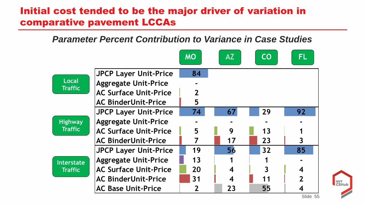
Slide 55
Initial cost tended to be the major driver of variation in
comparative pavement LCCAs
JPCP Layer Unit-Price 84
Aggregate Unit-Price -
AC Surface Unit-Price 2
AC BinderUnit-Price 5
JPCP Layer Unit-Price 74 67 29 92
Aggregate Unit-Price - - - -
AC Surface Unit-Price 5 9 13 1
AC BinderUnit-Price 7 17 23 3
JPCP Layer Unit-Price 19 56 32 85
Aggregate Unit-Price 13 1 1 -
AC Surface Unit-Price 20 4 3 4
AC BinderUnit-Price 31 4 11 2
AC Base Unit-Price 2 23 55 4
Local
Traffic
Highway
Traffic
Interstate
Traffic
MO AZ CO FL
Parameter Percent Contribution to Variance in Case Studies
Slide 56
Thoughts on implementing LCCA
• Key needs
– Established methodology
– Data
– Buy-in from stakeholders and support leaders
• Developing method
– Learn from others, but carry out stakeholder input process
• Invest in data collection
• Support those charged with the task
Slide 57
Initial cost variation questions
• Can we reduce variation?
– Incorporate new factors
• Quantity: Weight, volume, area, thickness
• Location: variability within a state
• Competition: Bids, AD/AB
– Evaluate alternative methodologies
• Weighted Least Square
• Regression trees
Slide 58
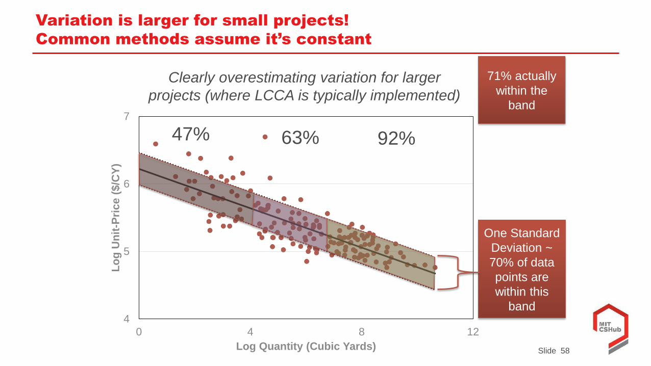
Variation is larger for small projects!
Common methods assume it’s constant
4
5
6
7
0 4 8 12
Lo
g U
nit
-Pri
ce (
$/C
Y)
Log Quantity (Cubic Yards)
One Standard
Deviation ~
70% of data
points are
within this
band
71% actually
within the
band
47% 63% 92%
Clearly overestimating variation for larger
projects (where LCCA is typically implemented)
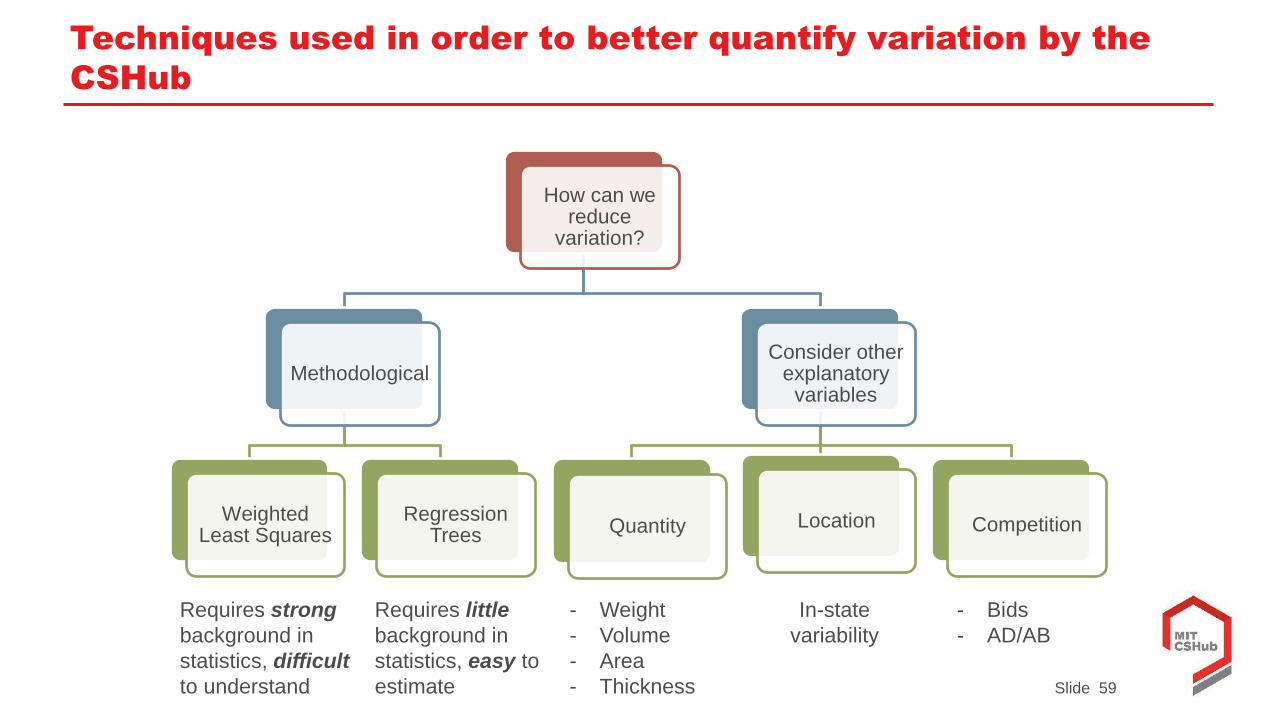
Slide 59
Techniques used in order to better quantify variation by the
CSHub
How can we reduce
variation?
Methodological
Weighted Least Squares
Regression Trees
Consider other explanatory
variables
Quantity Location Competition
Requires strong
background in
statistics, difficult
to understand
Requires little
background in
statistics, easy to
estimate
- Weight
- Volume
- Area
- Thickness
In-state
variability
- Bids
- AD/AB
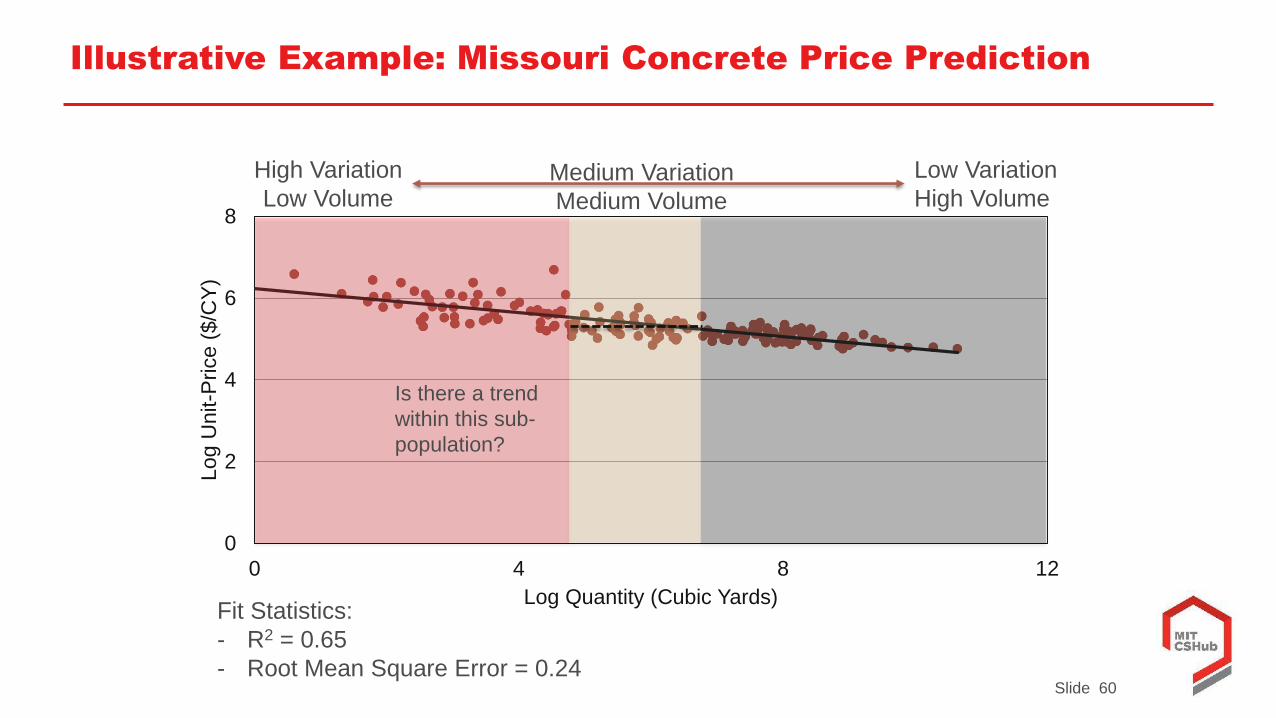
Slide 60
0
2
4
6
8
0 4 8 12
Log U
nit-P
rice (
$/C
Y)
Log Quantity (Cubic Yards)
Illustrative Example: Missouri Concrete Price Prediction
Fit Statistics:
- R2 = 0.65
- Root Mean Square Error = 0.24
High Variation
Low Volume
Low Variation
High VolumeMedium Variation
Medium Volume
Is there a trend
within this sub-
population?
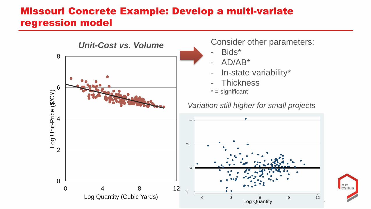
Slide 61
Missouri Concrete Example: Develop a multi-variate
regression model
Unit-Cost vs. Volume Consider other parameters:
- Bids*
- AD/AB*
- In-state variability*
- Thickness* = significant
-.5
0.5
1
Diff
ere
nce
Betw
ee
n A
ctua
l an
d P
red
icte
d
0 3 6 9 12
Log Quantity
Variation still higher for small projects
0
2
4
6
8
0 4 8 12
Log U
nit-P
rice (
$/C
Y)
Log Quantity (Cubic Yards)
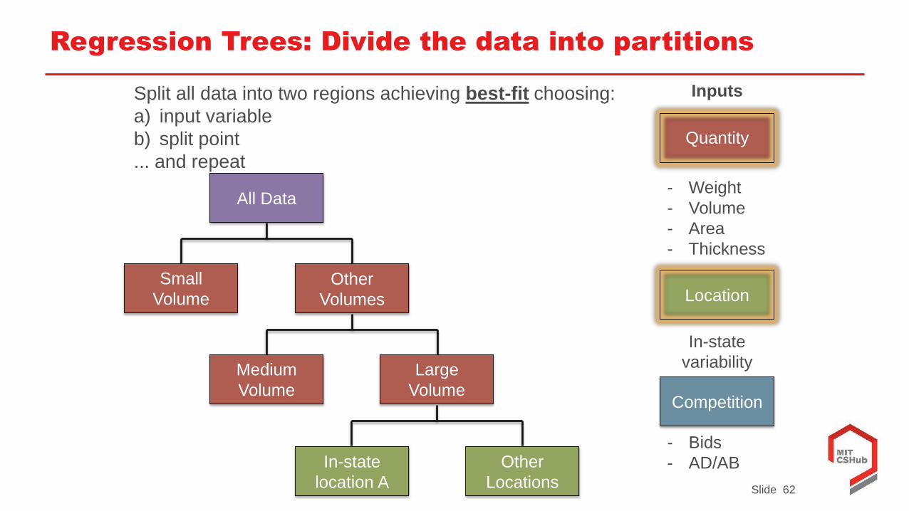
Slide 62
Regression Trees: Divide the data into partitions
Quantity
Location
Competition
Inputs
All Data
Small
Volume
Other
Volumes
Medium
Volume
Large
Volume
Other
Locations
In-state
location A
Split all data into two regions achieving best-fit choosing:
a) input variable
b) split point
... and repeat
- Weight
- Volume
- Area
- Thickness
In-state
variability
- Bids
- AD/AB
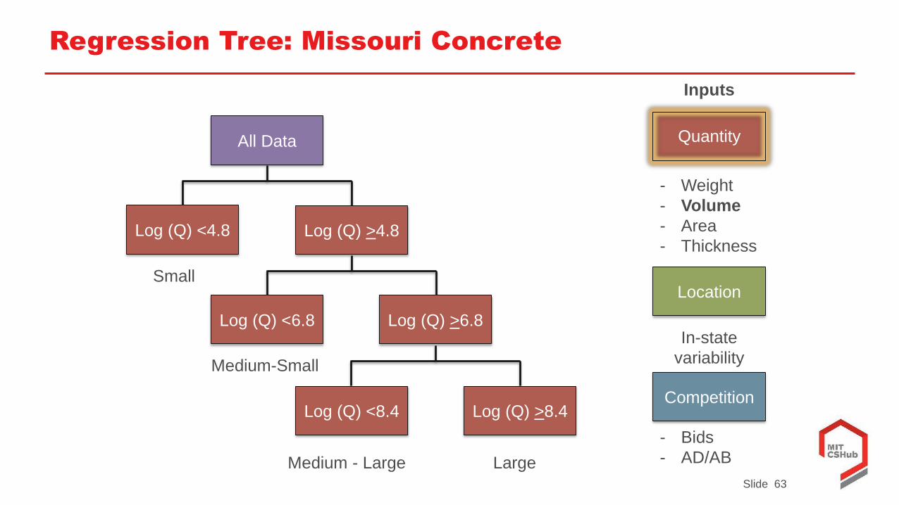
Slide 63
Regression Tree: Missouri Concrete
All Data
Log (Q) <4.8 Log (Q) >4.8
Log (Q) <6.8 Log (Q) >6.8
Log (Q) >8.4Log (Q) <8.4
Small
Medium-Small
Medium - Large Large
Quantity
Location
Competition
Inputs
- Weight
- Volume
- Area
- Thickness
In-state
variability
- Bids
- AD/AB
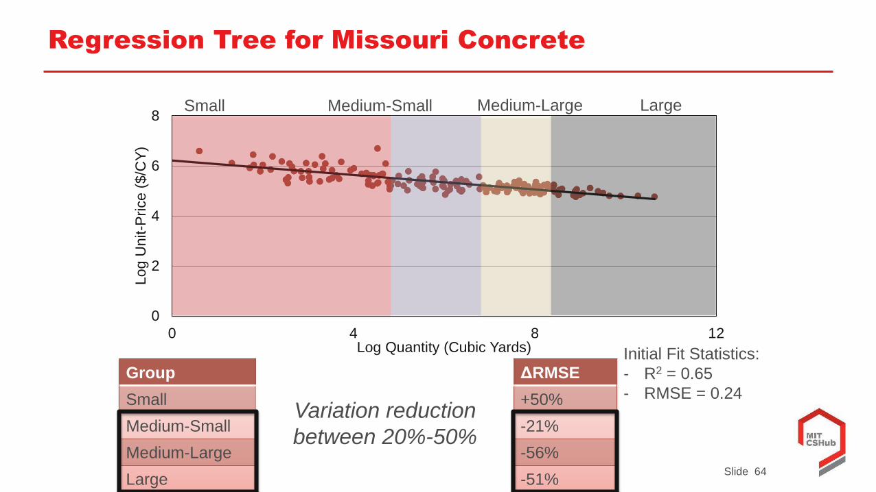
Slide 64
0
2
4
6
8
0 4 8 12
Log U
nit-P
rice (
$/C
Y)
Log Quantity (Cubic Yards)
Regression Tree for Missouri Concrete
Small Medium-Small Medium-Large Large
Group Significant Inputs RMSE ΔRMSE
Small None 0.36 +50%
Medium-Small Location 0.19 -21%
Medium-Large Location, Bids 0.11 -56%
Large None 0.12 -51%
Initial Fit Statistics:
- R2 = 0.65
- RMSE = 0.24Variation reduction
between 20%-50%
Slide 65
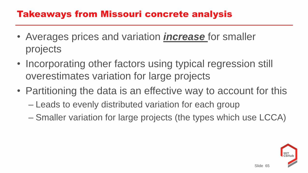
Takeaways from Missouri concrete analysis
• Averages prices and variation increase for smaller
projects
• Incorporating other factors using typical regression still
overestimates variation for large projects
• Partitioning the data is an effective way to account for this
– Leads to evenly distributed variation for each group
– Smaller variation for large projects (the types which use LCCA)
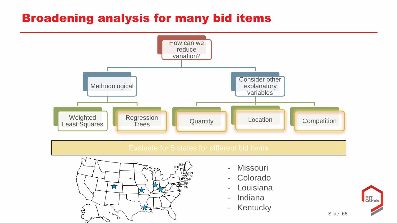
Slide 66
How can we reduce
variation?
Methodological
Weighted Least Squares
Regression Trees
Consider other explanatory
variables
Quantity Location Competition
Broadening analysis for many bid items
- Missouri
- Colorado
- Louisiana
- Indiana
- Kentucky
Evaluate for 5 states for different bid items
Slide 67
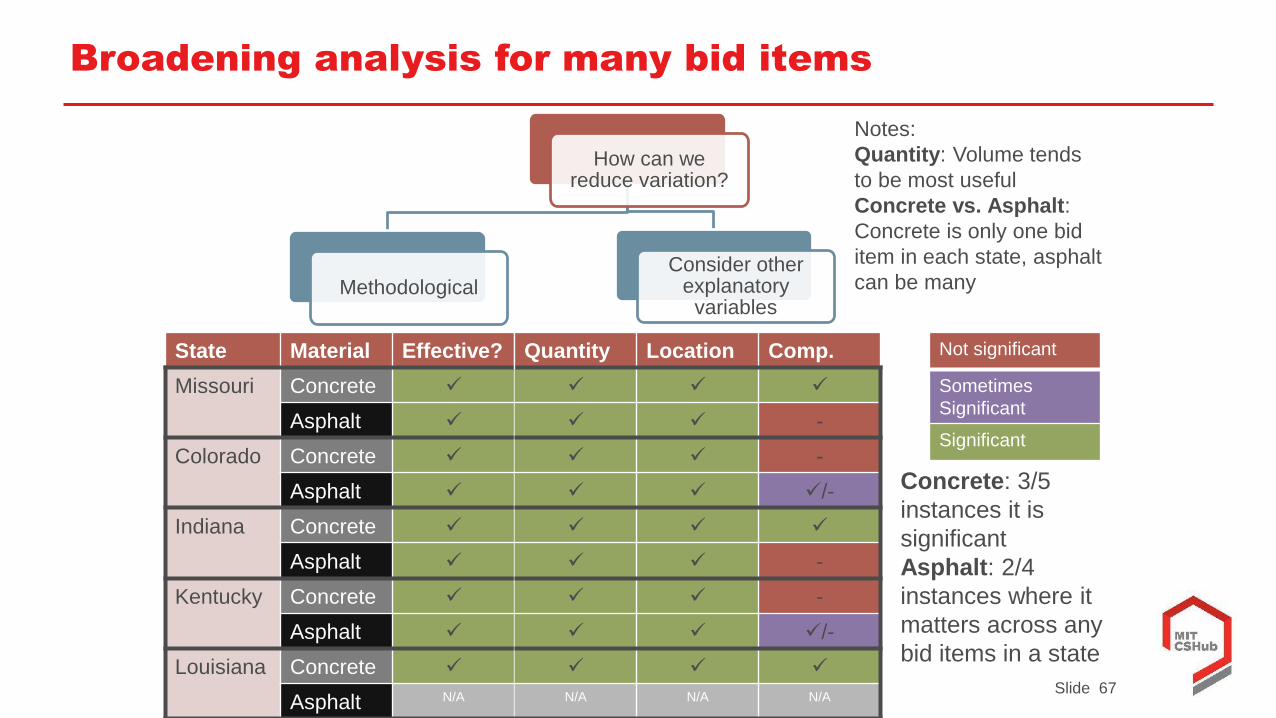
Broadening analysis for many bid items
How can we reduce variation?
MethodologicalConsider other
explanatory variables
State Material Effective?
Missouri Concrete
Asphalt
Colorado Concrete
Asphalt
Indiana Concrete
Asphalt
Kentucky Concrete
Asphalt
Louisiana Concrete
Asphalt N/A
Quantity Location Comp.
-
-
/-
-
-
/-
N/A N/A N/A
Not significant
Sometimes
Significant
Significant
Concrete: 3/5
instances it is
significant
Asphalt: 2/4
instances where it
matters across any
bid items in a state
Notes:
Quantity: Volume tends
to be most useful
Concrete vs. Asphalt:
Concrete is only one bid
item in each state, asphalt
can be many
Slide 68
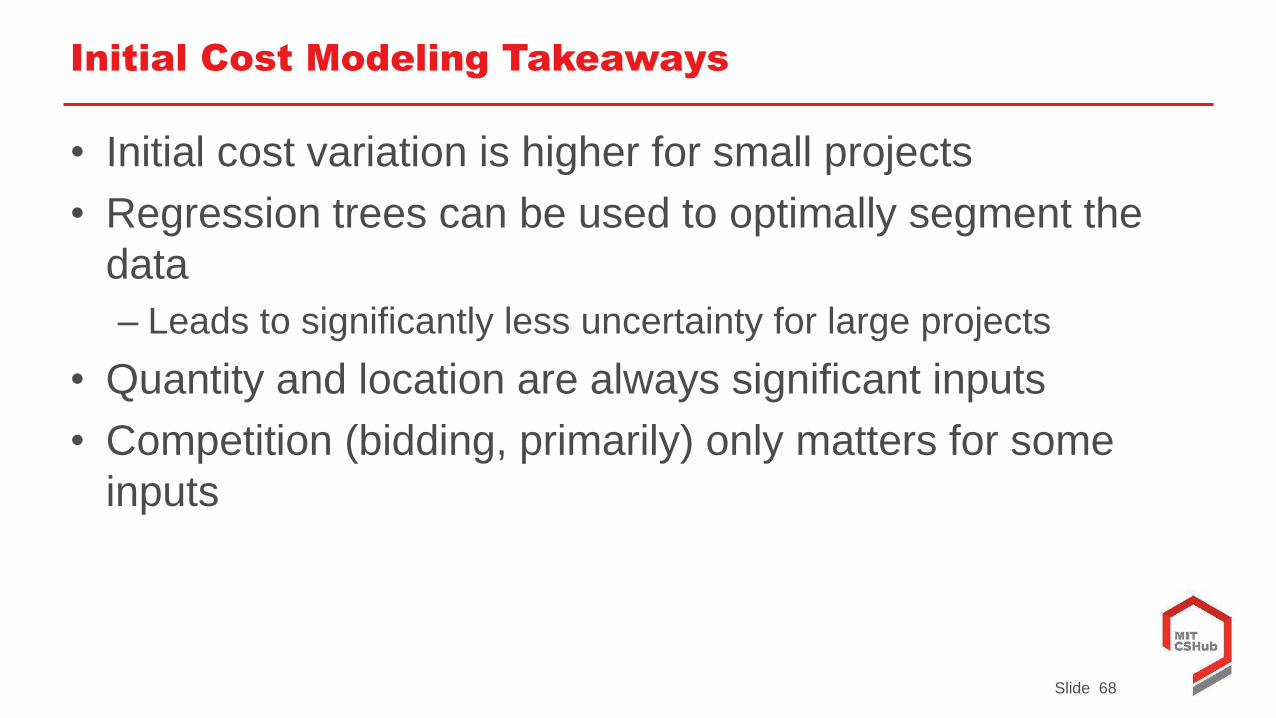
Initial Cost Modeling Takeaways
• Initial cost variation is higher for small projects
• Regression trees can be used to optimally segment the
data
– Leads to significantly less uncertainty for large projects
• Quantity and location are always significant inputs
• Competition (bidding, primarily) only matters for some
inputs

Slide 69
Asset Management
Slide 70
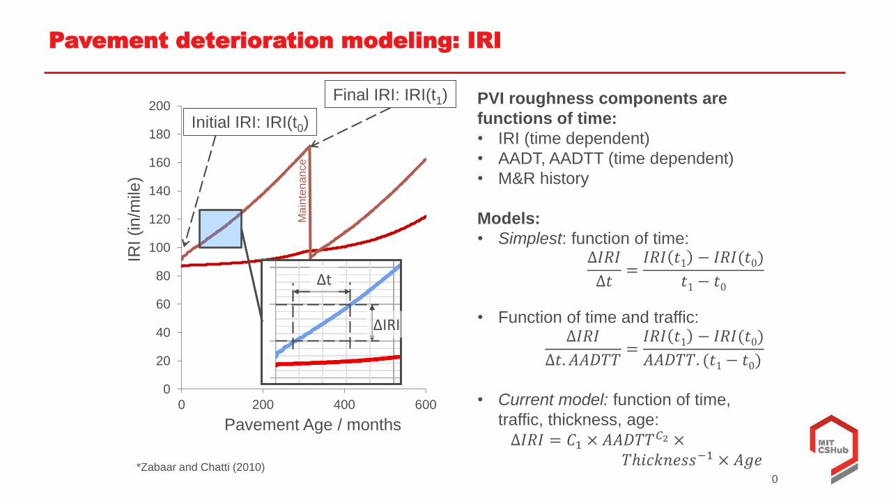
Pavement deterioration modeling: IRI
0
20
40
60
80
100
120
140
160
180
200
0 200 400 600
Pavement Age / months
IRI (in/m
ile)
Ma
inte
nan
ce
Δt
ΔIRI
Final IRI: IRI(t1)
Initial IRI: IRI(t0)
PVI roughness components are
functions of time:
• IRI (time dependent)
• AADT, AADTT (time dependent)
• M&R history
Models:
• Simplest: function of time:∆𝐼𝑅𝐼
∆𝑡=𝐼𝑅𝐼 𝑡1 − 𝐼𝑅𝐼(𝑡0)
𝑡1− 𝑡0
• Function of time and traffic:∆𝐼𝑅𝐼
∆𝑡. 𝐴𝐴𝐷𝑇𝑇=𝐼𝑅𝐼 𝑡1 − 𝐼𝑅𝐼(𝑡0)
𝐴𝐴𝐷𝑇𝑇. (𝑡1− 𝑡0)
• Current model: function of time,
traffic, thickness, age:
∆𝐼𝑅𝐼 = 𝐶1 × 𝐴𝐴𝐷𝑇𝑇𝐶2 ×𝑇ℎ𝑖𝑐𝑘𝑛𝑒𝑠𝑠−1 × 𝐴𝑔𝑒
*Zabaar and Chatti (2010)
Slide 71
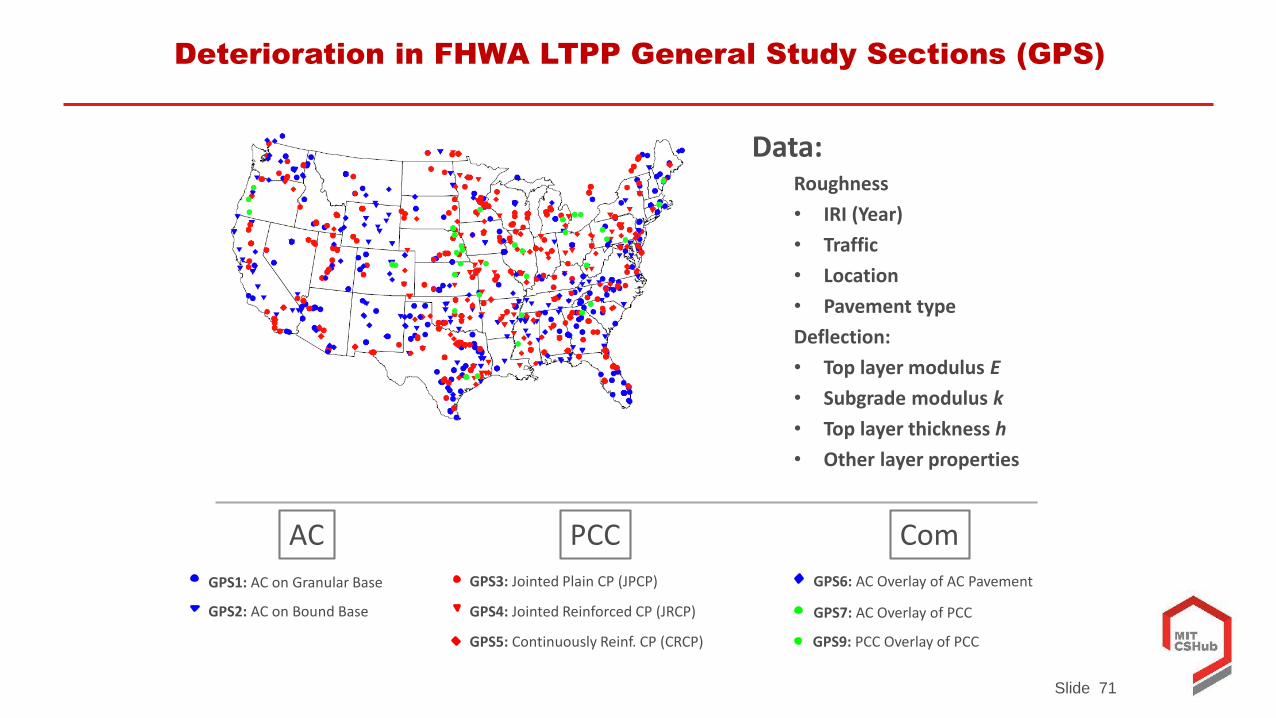
Deterioration in FHWA LTPP General Study Sections (GPS)
Data:Roughness
• IRI (Year)
• Traffic
• Location
• Pavement type
Deflection:
• Top layer modulus E
• Subgrade modulus k
• Top layer thickness h
• Other layer properties
GPS1: AC on Granular Base
GPS2: AC on Bound Base
GPS3: Jointed Plain CP (JPCP)
GPS4: Jointed Reinforced CP (JRCP)
GPS5: Continuously Reinf. CP (CRCP)
GPS6: AC Overlay of AC Pavement
GPS7: AC Overlay of PCC
GPS9: PCC Overlay of PCC
AC ComPCC
Slide 72
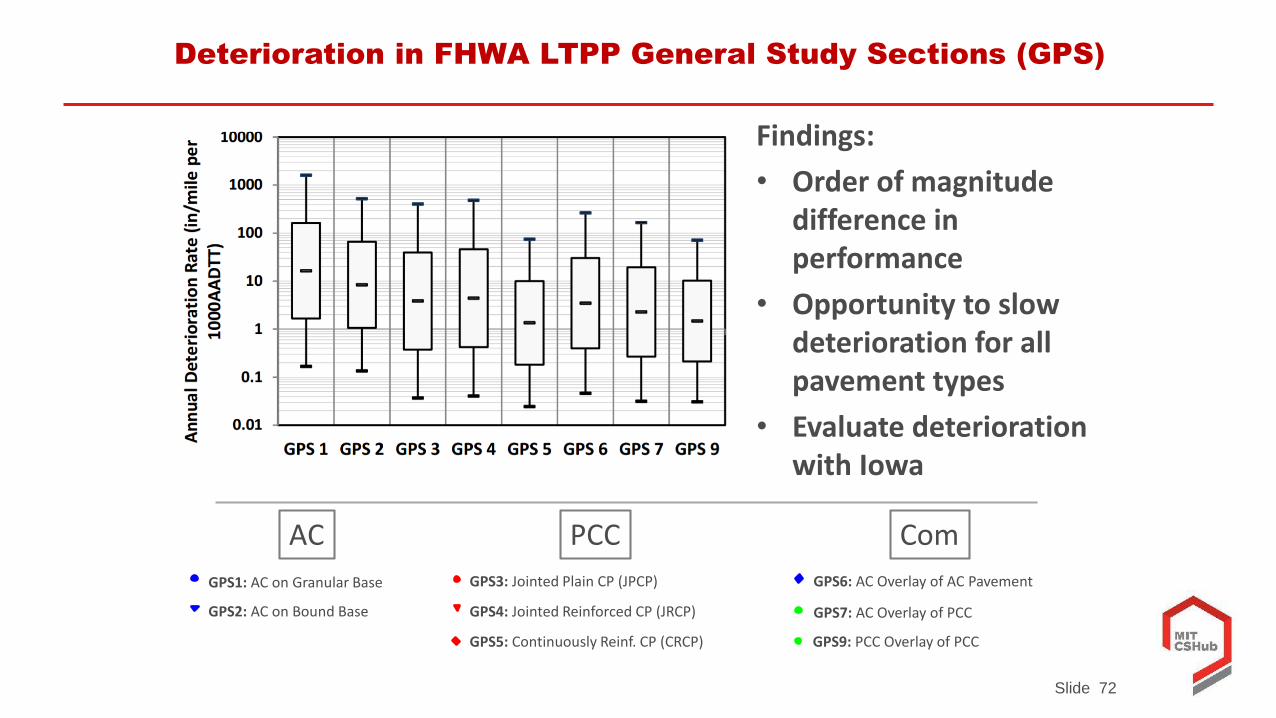
Deterioration in FHWA LTPP General Study Sections (GPS)
Findings:
• Order of magnitude difference in performance
• Opportunity to slow deterioration for all pavement types
• Evaluate deterioration with Iowa
GPS1: AC on Granular Base
GPS2: AC on Bound Base
GPS3: Jointed Plain CP (JPCP)
GPS4: Jointed Reinforced CP (JRCP)
GPS5: Continuously Reinf. CP (CRCP)
GPS6: AC Overlay of AC Pavement
GPS7: AC Overlay of PCC
GPS9: PCC Overlay of PCC
AC ComPCC

Slide 73
MIT probabilistic network allocation model
Allocation
Optimization
Tool
Current state of
system
Projection models
of future
conditions
A set of
objectives/goals
Available MRR
actions
Objective: find allocation policy
that maximizes expected
performance or minimizes cost
Project Resource
Allocation
Computationally
efficient algorithm
Slide 74
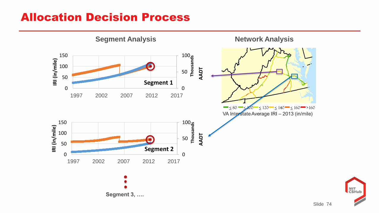
Allocation Decision Process
0
50
100
0
50
100
150
0 200 400 600 800
AA
DT
Th
ou
san
ds
IRI (
in/m
ile)
Segment 1
0
50
100
0
50
100
150
0 200 400 600 800
AA
DT
Tho
usa
nd
s
IRI (
in/m
ile)
Segment 2
1997 2002 2007 2012 2017
1997 2002 2007 2012 2017
Segment 3, ….
Segment Analysis Network Analysis
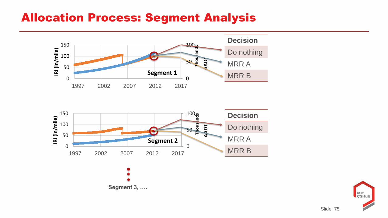
Slide 75
Allocation Process: Segment Analysis
0
50
100
0
50
100
150
0 200 400 600 800
AA
DT
Tho
usa
nd
s
IRI (
in/m
ile)
Segment 1
0
50
100
0
50
100
150
0 200 400 600 800
AA
DT
Tho
usa
nd
s
IRI (
in/m
ile)
Segment 2
1997 2002 2007 2012 2017
1997 2002 2007 2012 2017
Segment 3, ….
Decision
Do nothing
MRR A
MRR B
Decision
Do nothing
MRR A
MRR B
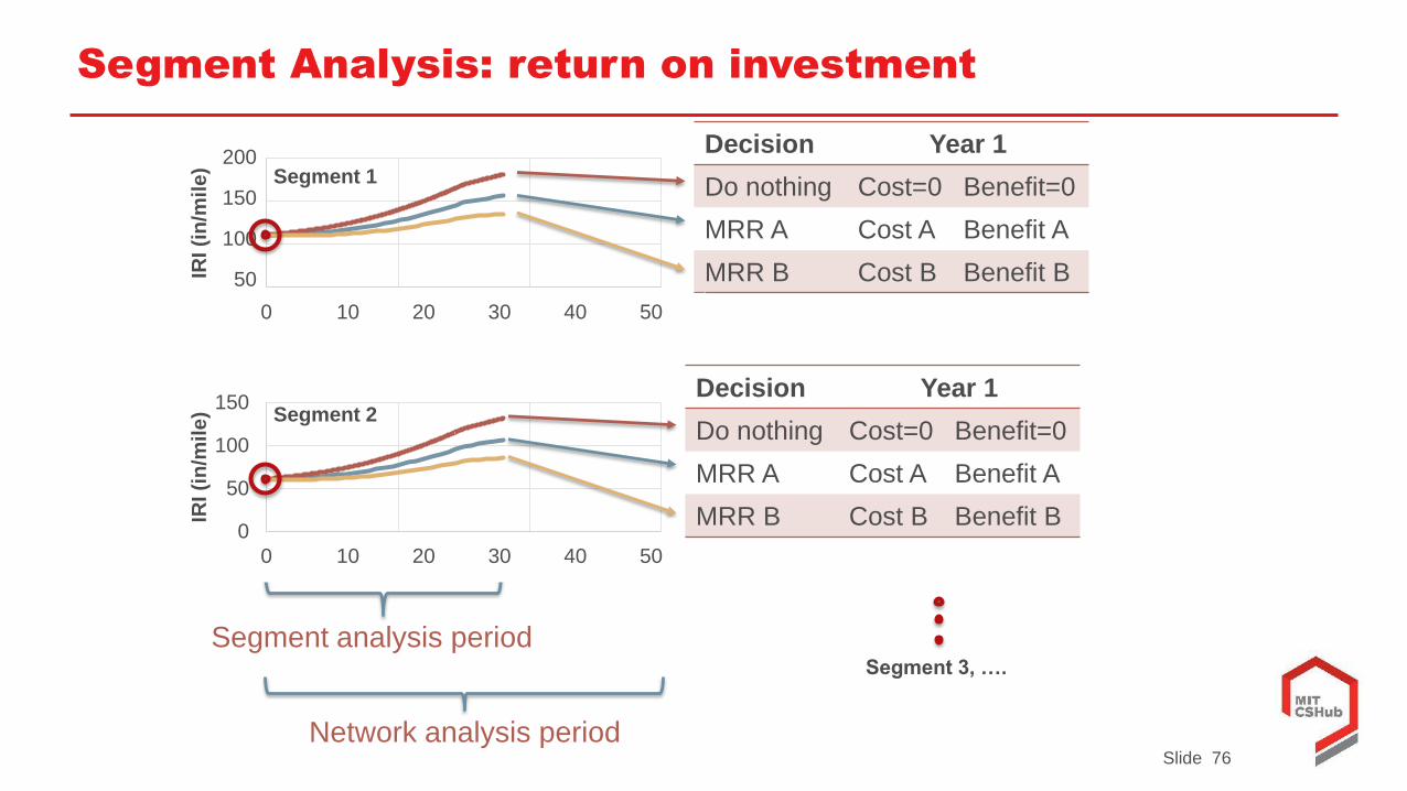
Slide 76
Segment Analysis: return on investment
Decision Year 1
Do nothing Cost=0 Benefit=0
MRR A Cost A Benefit A
MRR B Cost B Benefit B
Segment analysis period
0
50
100
150
0 200 400 600
IRI (i
n/m
ile
)
0 10 20 30 40 50
0
50
100
150
0 200 400 600
IRI (i
n/m
ile
)
0 10 20 30 40 50
200
150
100
50
Network analysis period
Decision Year 1
Do nothing Cost=0 Benefit=0
MRR A Cost A Benefit A
MRR B Cost B Benefit B
Segment 1
Segment 2
Segment 3, ….
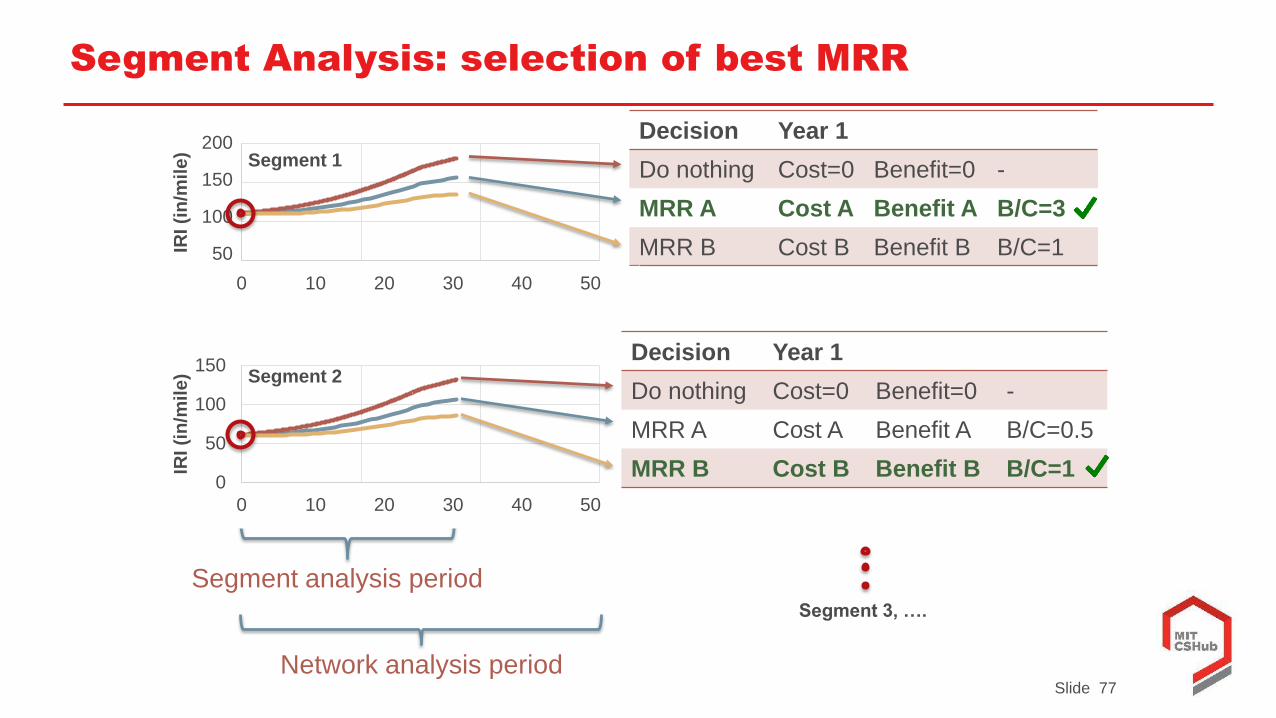
Slide 77
Segment Analysis: selection of best MRR
Decision Year 1
Do nothing Cost=0 Benefit=0 -
MRR A Cost A Benefit A B/C=3
MRR B Cost B Benefit B B/C=1
Segment analysis period
0
50
100
150
0 200 400 600
IRI (i
n/m
ile
)
0 10 20 30 40 50
0
50
100
150
0 200 400 600
IRI (i
n/m
ile
)
0 10 20 30 40 50
200
150
100
50
Network analysis period
Decision Year 1
Do nothing Cost=0 Benefit=0 -
MRR A Cost A Benefit A B/C=0.5
MRR B Cost B Benefit B B/C=1
Segment 1
Segment 2
Segment 3, ….
Slide 78
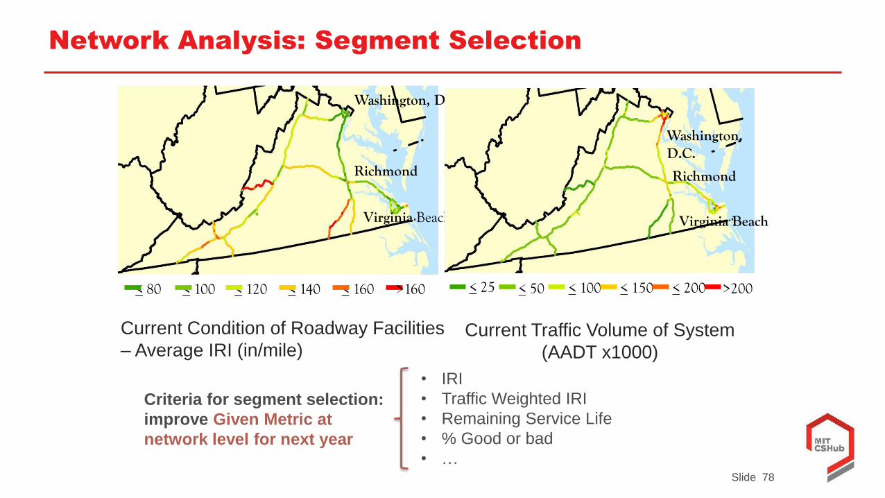
Network Analysis: Segment Selection
Washington, D.C.
Richmond
Virginia Beach
< 80 < 100 < 120 < 140 < 160 >160
Washington,D.C.
Richmond
Virginia Beach
< 25 < 50 < 100 < 150 < 200 >200
Current Traffic Volume of System
(AADT x1000)
Current Condition of Roadway Facilities
– Average IRI (in/mile)
Criteria for segment selection:
improve Given Metric at
network level for next year
• IRI
• Traffic Weighted IRI
• Remaining Service Life
• % Good or bad
• …
Slide 79
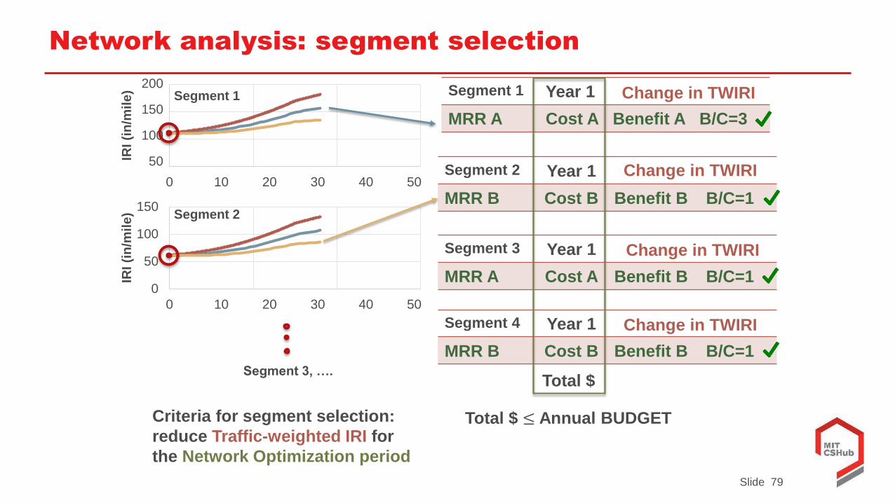
Network analysis: segment selection
Segment 1 Year 1
MRR A Cost A Benefit A B/C=3
0
50
100
150
0 200 400 600
IRI (i
n/m
ile
)
0 10 20 30 40 50
0
50
100
150
0 200 400 600
IRI (i
n/m
ile
)
0 10 20 30 40 50
200
150
100
50Segment 2 Year 1
MRR B Cost B Benefit B B/C=1
Segment 1
Segment 2
Total $
Total $ ≤ Annual BUDGETCriteria for segment selection:
reduce Traffic-weighted IRI for
the Network Optimization period
Segment 3, ….
Segment 3 Year 1
MRR A Cost A Benefit B B/C=1
Segment 4 Year 1
MRR B Cost B Benefit B B/C=1
Change in TWIRI
Change in TWIRI
Change in TWIRI
Change in TWIRI
Slide 80
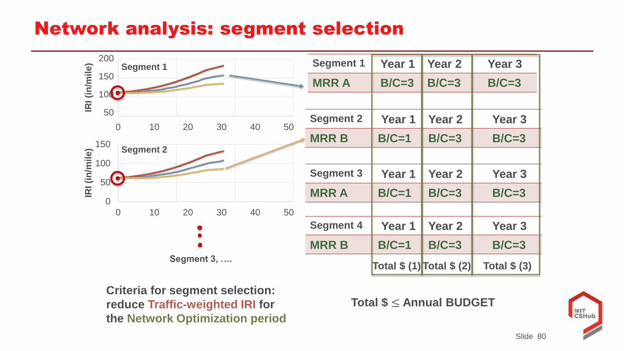
Network analysis: segment selection
Segment 1 Year 1 Year 2 Year 3
MRR A B/C=3 B/C=3 B/C=3
0
50
100
150
0 200 400 600
IRI (i
n/m
ile
)
0 10 20 30 40 50
0
50
100
150
0 200 400 600
IRI (i
n/m
ile
)
0 10 20 30 40 50
200
150
100
50Segment 2 Year 1 Year 2 Year 3
MRR B B/C=1 B/C=3 B/C=3
Segment 1
Segment 2
Total $ (1)
Total $ ≤ Annual BUDGETCriteria for segment selection:
reduce Traffic-weighted IRI for
the Network Optimization period
Segment 3, ….
Segment 3 Year 1 Year 2 Year 3
MRR A B/C=1 B/C=3 B/C=3
Segment 4 Year 1 Year 2 Year 3
MRR B B/C=1 B/C=3 B/C=3
Total $ (2) Total $ (3)
Slide 81
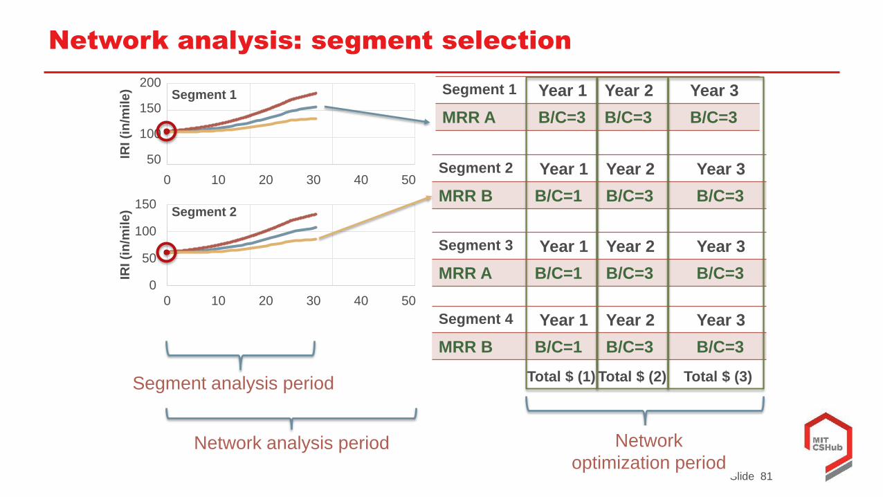
Network analysis: segment selection
Segment 1 Year 1 Year 2 Year 3
MRR A B/C=3 B/C=3 B/C=3
0
50
100
150
0 200 400 600
IRI (i
n/m
ile
)
0 10 20 30 40 50
0
50
100
150
0 200 400 600
IRI (i
n/m
ile
)
0 10 20 30 40 50
200
150
100
50Segment 2 Year 1 Year 2 Year 3
MRR B B/C=1 B/C=3 B/C=3
Segment 1
Segment 2
Total $ (1)
Segment 3 Year 1 Year 2 Year 3
MRR A B/C=1 B/C=3 B/C=3
Segment 4 Year 1 Year 2 Year 3
MRR B B/C=1 B/C=3 B/C=3
Total $ (2) Total $ (3)Segment analysis period
Network analysis period Network
optimization period