Doing Experiments in PhysicsDoing Experiments in Physics

Shirish R. PathareShirish R. Pathare

Homi Bhabha Centre for Science EducationTata Institute of Fundamental Research

V. N. Purav Marg, Mankhurd. Mumbai – 400 088.

shirish@hbcse.tifr.res.in

We can think of experimental work in physics as consisting of the following steps:

Conceptualization

Data collection

Data processing and analysis

Inferences and conclusions

Experimental Work in PhysicsExperimental Work in Physics

Conceptualization of ExperimentConceptualization of Experiment

In analyzing a phenomenon one first tries to identify the physical quantities that are involved in the phenomenon.

Think of ways to keep all except one variable constant and observe the phenomenon by varying it in a systematic way.

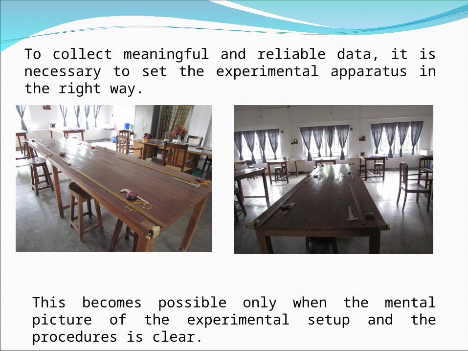
To collect meaningful and reliable data, it is necessary to set the experimental apparatus in the right way.

This becomes possible only when the mental picture of the experimental setup and the procedures is clear.

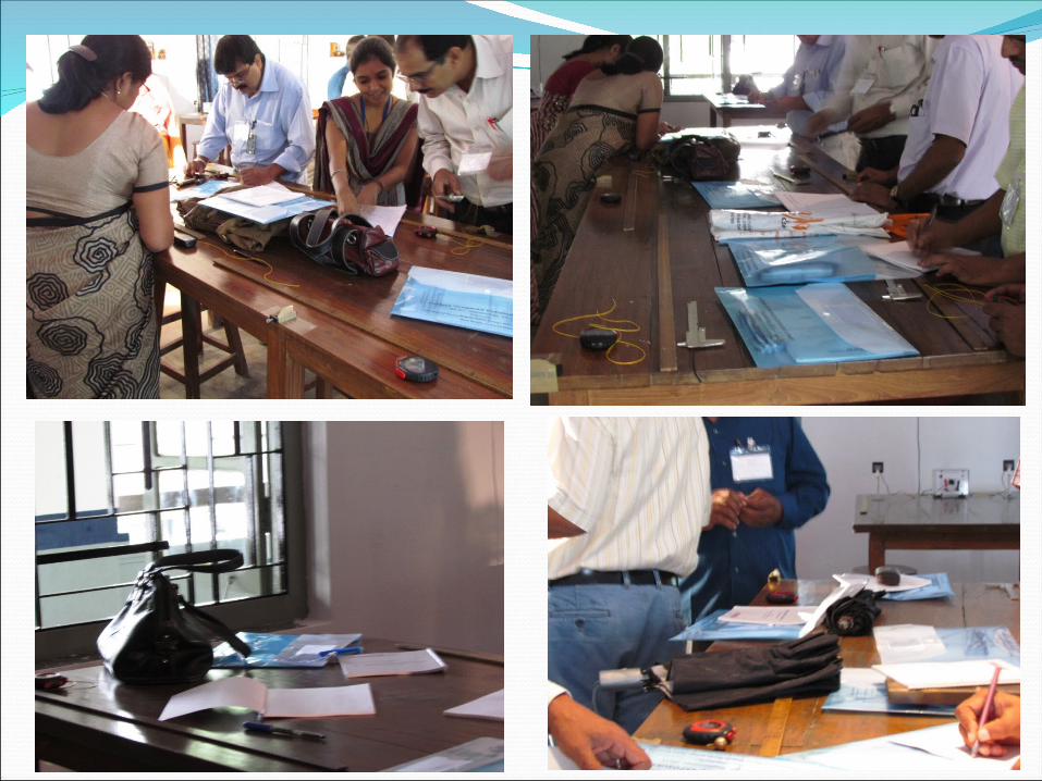
Verniers…Why?Verniers…Why?

… so Conceptualization of the experiment consists of thinking about

the objective of the experiment,

the principles of physics involved,

the procedures to be followed in the measurements and

the arrangement of the apparatus.

It is also essential to plan about the range of independent variable over which the data is to be collected and the appropriate precisions (or least counts) of the measuring instruments.

To make proper choice of measuring instruments with appropriate precisions, sensitivity analysis using the formula of propagation of uncertainty in the result is helpful.

Each quantity measured in the experiment has some uncertainty in the measured value.

So, the best one can do is to see that contributions to the uncertainty in the result from them are of the same order.

e.g.In the case of simple pendulum, the uncertainty in the measurement of length, l and the uncertainty in the measurement of time t should be of same order.

As a primary goal the choice of precision of measuring instrument must be such that the uncertainty in the measured value is less than 1%.

How is the uncertainty in measurement related to the precision or resolution of the measuring instrument?

The readings of the instrument are multiples of the smallest unit (least count) of the scale.

Any fraction of the least count cannot be included in the reading.

Thus the measurement is uncertain to the extent of that unmeasured part and so is dependent on the resolution of the measuring instrument.

Every measuring instrument has some scale with markings or digital display.

To keep the uncertainty due to the limit of resolution of the measuring device less than 1% …

How many oscillations should we choose to measure the time interval to determine the periodic time of a simple pendulum?

… the choice of either the measured quantity or the measuring instrument must be such that the reading is at least 100 units of least count.

The answer to this question depends upon the resolution of the watch as well as some other considerations.

Least count of the stopwatch used = 0.01 s

Hence to limit the uncertainty below 1% in the reading due to this least count of 0.01 s,

the minimum interval could be … 1 s !!!

So one oscillation should be enough.Then why waste so much of time by choosing an interval with more oscillations…???

See what values you get for the period of the pendulum by repeating the measurement.

Is it possible to achieve repeatability in the readings using the watch with least count of 0.01 s ???

No. The measurements vary randomly. We cannot know the true value of the measured quantity because of the random errors present.

This is done by either truncating the reading to ignore the last digit or rounding the previous digit in the reading of the watch. By this we have increased our uncertainty to such an extent that the random errors are now smaller than it.

With this least count the minimum time interval to limit the uncertainty below 1% would be 10 s.

Knowing the approximate period determine the number of oscillations in an interval of 10 s, and then choose some round number N above that for your measurements.

The most important thinking exercise is about searching possible sources of systematic errors in the data and devise methods to apply corrections for those errors. Sound theoretical knowledge about all things involved in the experiment is essential for this search.

Random errors change the readings when repeated and thus their presence can easily be detected.

But suppose the watch is running slow. Then the time measured may show same readings when repeated. The error cannot be detected from repeating the readings because it remains constant and does not change randomly.

Such errors are called systematic errors.

Systematic errors generally produce changes in the readings in the same direction.

They may be due to incorrect setting of the apparatus, wrong procedures followed in taking readings, faulty instruments and such other factors.

Some common systematic errors Some common systematic errors

Zero error in micrometer screw and vernier callipers readings.

The ‘backlash’ error. When the readings on a scale of microscope are taken by rotating the screw first in one direction and then in the reverse direction …

… the reading is less than the actual distance through which the screw is moved.

To avoid this error all the readings must be taken while rotating the screw in the same direction.

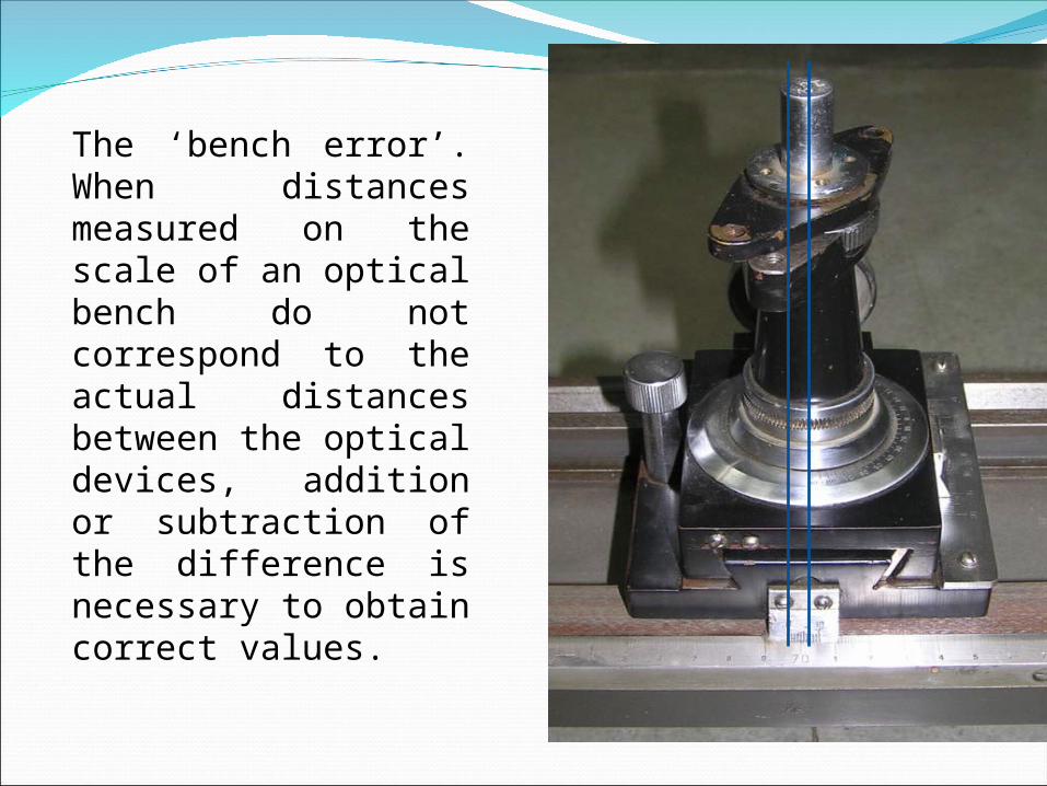
The ‘bench error’. When distances measured on the scale of an optical bench do not correspond to the actual distances between the optical devices, addition or subtraction of the difference is necessary to obtain correct values.

To detect systematic errors due to inaccurate apparatus or due to unsuspected effects of the apparatus in use,

one way is to replace the apparatus by another of similar type,

These steps will show if the calibrations of the instruments are inaccurate or if the instruments in some way produce some disturbances.

another is to make all such possible changes in the arrangement of the apparatus which are not expected to bring about any changes in the readings of the instruments and then observe if any changes are there. (e.g. unwanted magnetic or thermal or optical disturbances)

The deformation of a body under external forces is a slow process and is not instantaneous.

Similarly, when a substance is heated by keeping it in a constant temperature bath its temperature does not attain the temperature of the bath instantaneously.

Often the experimenter has to take readings without waiting for the steady state.

For this reason, the reading of extension of a wire for a particular load while loading will be less than corresponding reading while unloading.

Similarly, the reading of resistance of a thermistor while heating will be more than that while cooling at the same temperature.

The mean values of the two readings approximately eliminate this type of error.

This type of error depends on the direction of change of the quantity being measured and is called ‘error due to hysteresis’.

Data CollectionData Collection

The data should be collected first by varying the independent variable uniformly over the entire range of the study and then additional readings may be taken where the study is to be more specific.

The range of the study should be as wide as is permitted by the experimental set up.

If the relation between the independent variable and the dependent variable is expected to be linear, then six to eight readings are adequate.

Always state the absolute uncertainty in the readings while taking the readings.

More readings should not be taken if they do not provide any additional information, because that will be only waste of time and energy.

When the relation is non linear, after covering the entire range uniformly, more readings (by varying the independent variable) are needed to locate the points of maxima and minima, points of inflexion etc.

Additional necessary readings are to be taken wherever needed after examining the observations taken over the entire range.

LCR Series Resonance

Data Processing and Data AnalysisData Processing and Data Analysis

The data recorded from observation is to be processed to be able to draw inferences.

Often secondary data is created using the primary data and then it is used for analysis. While calculating this secondary data the uncertainties in them are also to be estimated.

Graph PlottingGraph Plotting

One efficient tool of analysis is graph plotting.

The independent variable (or secondary data obtained from it) is plotted on the x-axis and the corresponding data representing dependent variable on the y-axis.

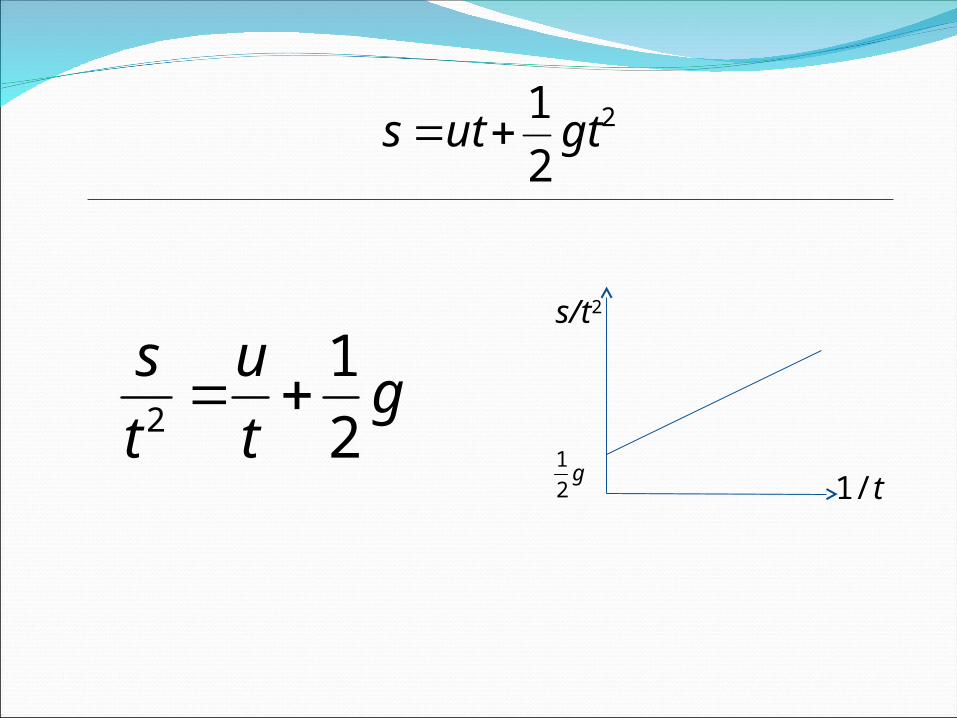
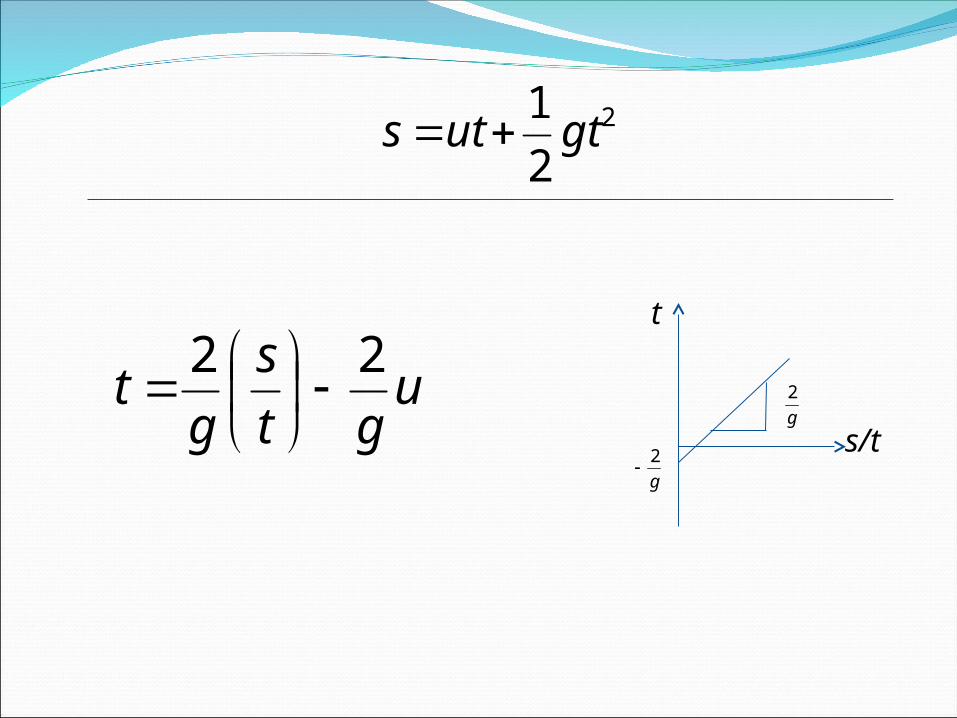
Often the primary data is combined in such a way that the relation plotted on the graph is linear. The linearizing of the relation is found to be useful to get the results from slopes and intercepts of graphs using all available data.

2

21 gtuts

ugtts

21

s/t

t

g21

2

21 gtuts

gtu

ts

21

2 s/t2

1/tg21

2

21 gtuts

ugt

sg

t 22

t

s/tg2

g2

2

21 gtuts

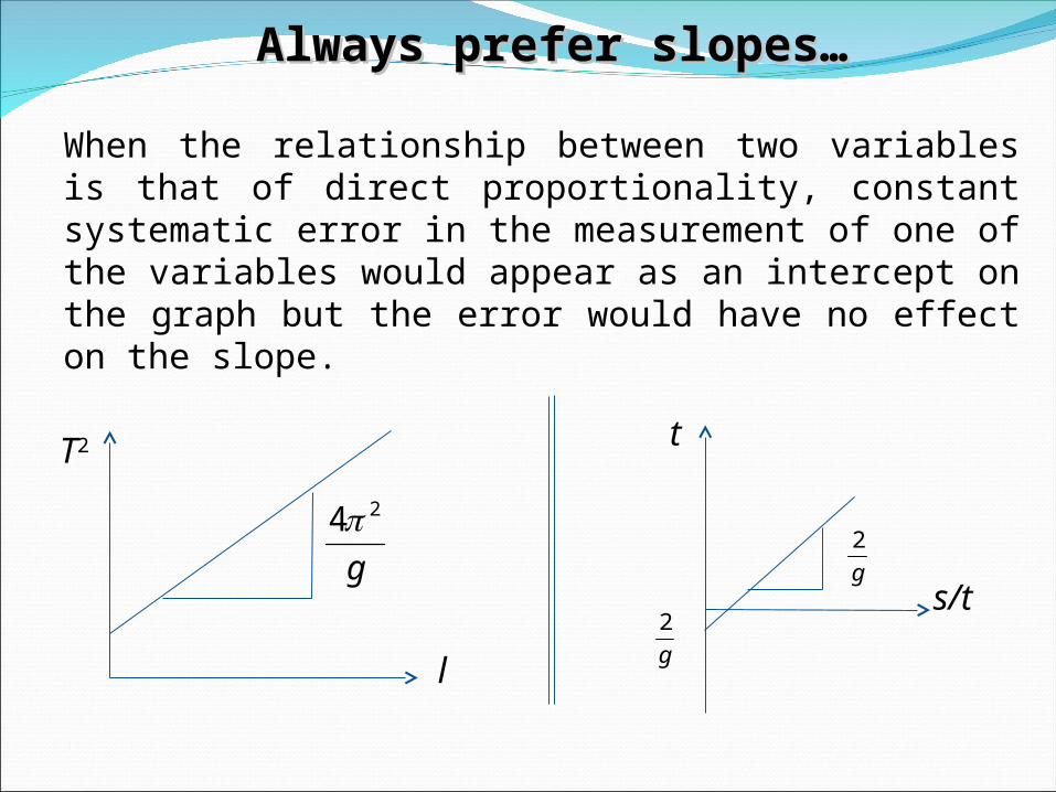
When the relationship between two variables is that of direct proportionality, constant systematic error in the measurement of one of the variables would appear as an intercept on the graph but the error would have no effect on the slope.

Always prefer slopes…Always prefer slopes…

T2

l

g

24

t

s/tg2

g2

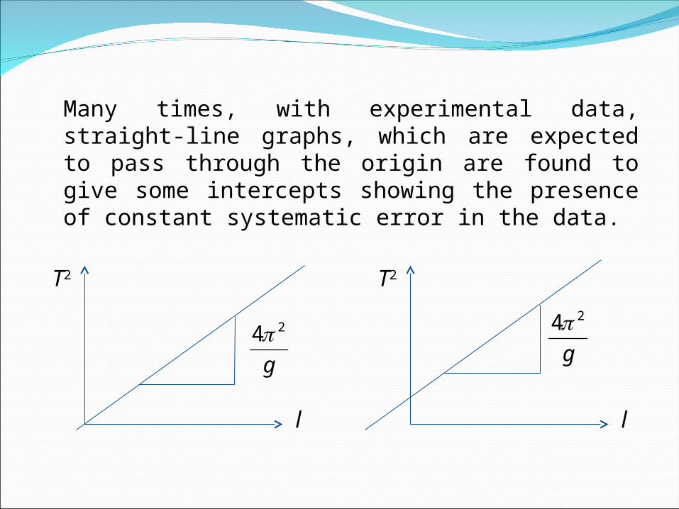
Many times, with experimental data, straight-line graphs, which are expected to pass through the origin are found to give some intercepts showing the presence of constant systematic error in the data.

T2

l

g

24

T2

l

g

24

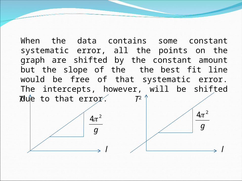
When the data contains some constant systematic error, all the points on the graph are shifted by the constant amount but the slope of the the best fit line would be free of that systematic error. The intercepts, however, will be shifted due to that error.

T2

l

g

24

T2

l

g

24

If calculations are made from the data, the error remains in the calculated result.

Hence, whenever a linear relationship is expected, the slope should be used in the formula instead of the mean of the ratios of the two quantities.

Calculation using the mean of the ratios includes the systematic error and should not be used.

By calculation By graph

×

If calculations are made from the data, the error remains in the calculated result.

Hence, whenever a linear relationship is expected, the slope should be used in the formula instead of the mean of the ratios of the two quantities.

Calculation using the mean of the ratios includes the systematic error and should not be used.

By calculation By graph

A few Graphs…

A few “Bad” Graphs…

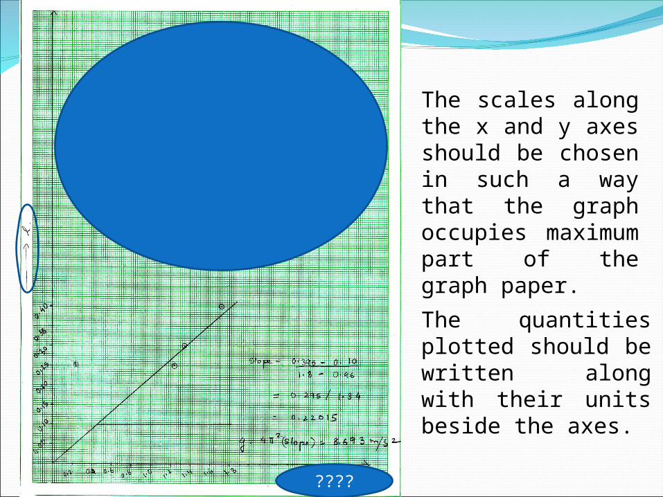
The scales along the x and y axes should be chosen in such a way that the graph occupies maximum part of the graph paper.

????

The quantities plotted should be written along with their units beside the axes.

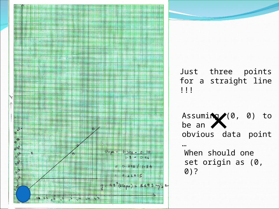
Assuming (0, 0) to be an obvious data point …

Just three points for a straight line !!!

When should one set origin as (0, 0)?

×

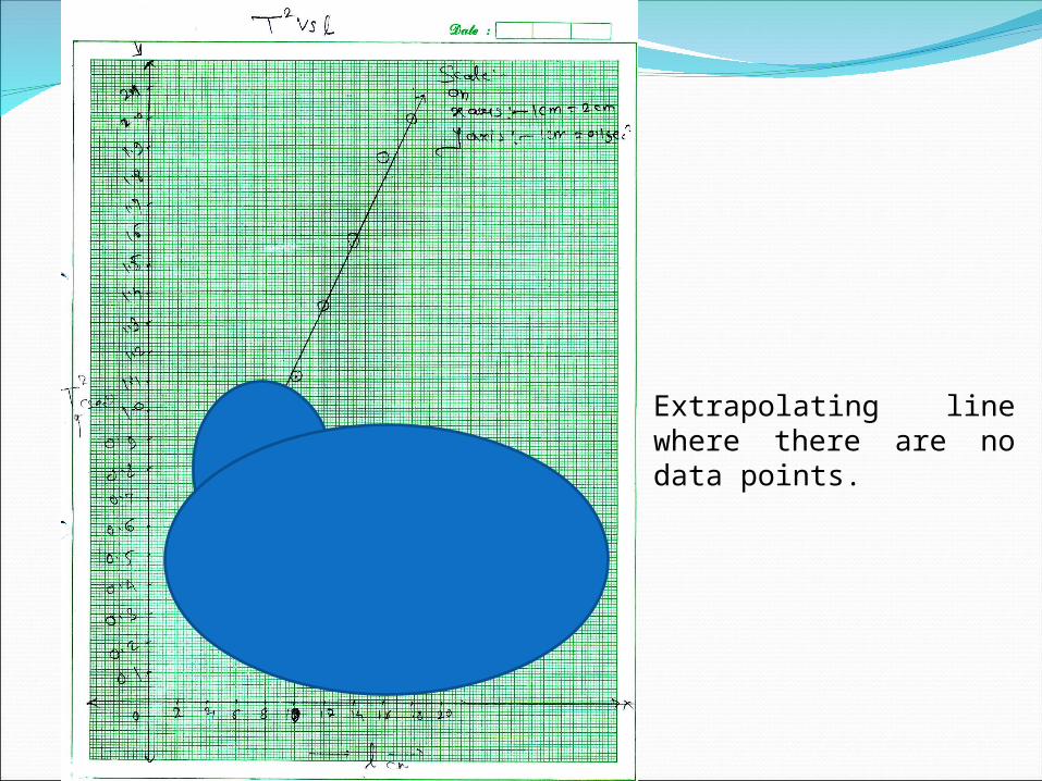
Extrapolating line where there are no data points.

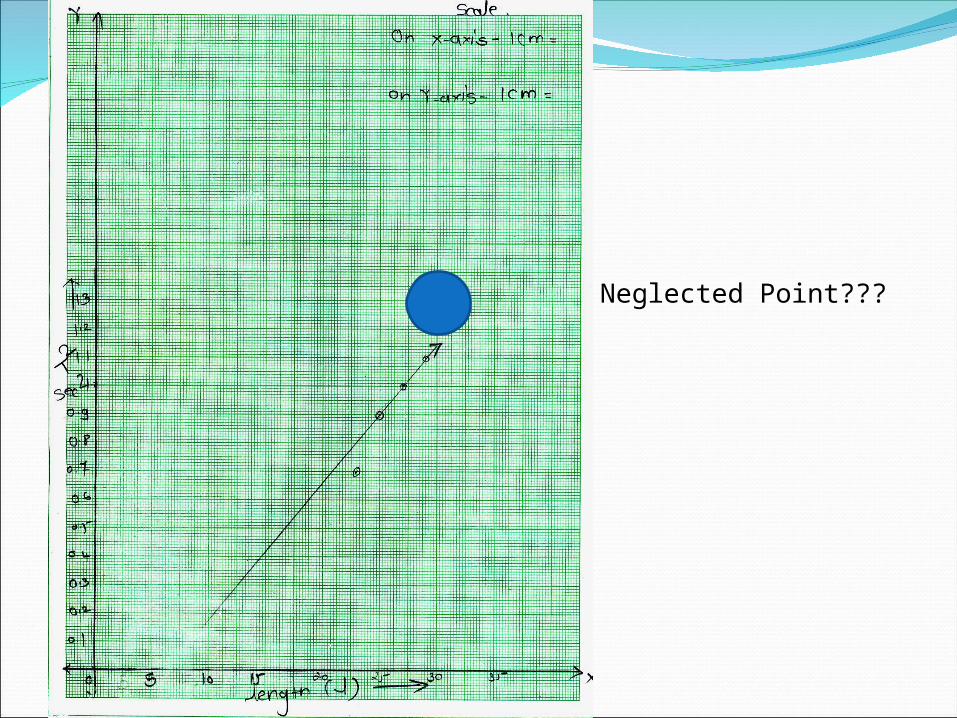
Neglected Point???

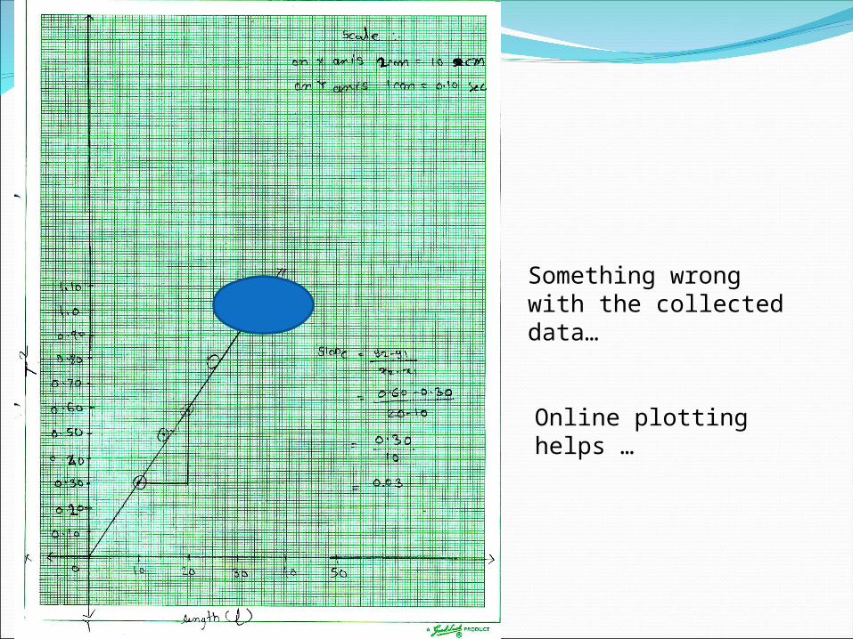
Something wrong with the collected data…

Online plotting helps …

The smallest unit on graph is a simple multiple of the unit of data.

Taking scale like 3 cm of graph paper equal to 1 unit of data makes life difficult.

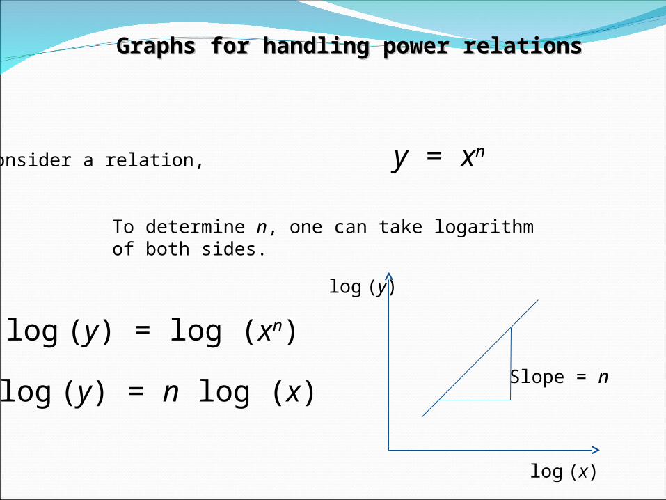
Graphs for handling power relationsGraphs for handling power relations

Consider a relation, y = xn

To determine n, one can take logarithm of both sides.

log (y) = log (xn)

log (y) = n log (x)

log (y)

log (x)

Slope = n

When the graph is supposed to be a straight line, it is essential to see which is the best fit line.

If we believe that there is only one line representing the data, then there will be no uncertainty in the slope of the line and it will mean that there is no error in data plotted.

…obviously, this can’t be correct.

If all the points appear to lie on a straight line then it is simple to identify the line by simply drawing the line passing through all the points.

Calculating Uncertainty from Calculating Uncertainty from GraphGraph

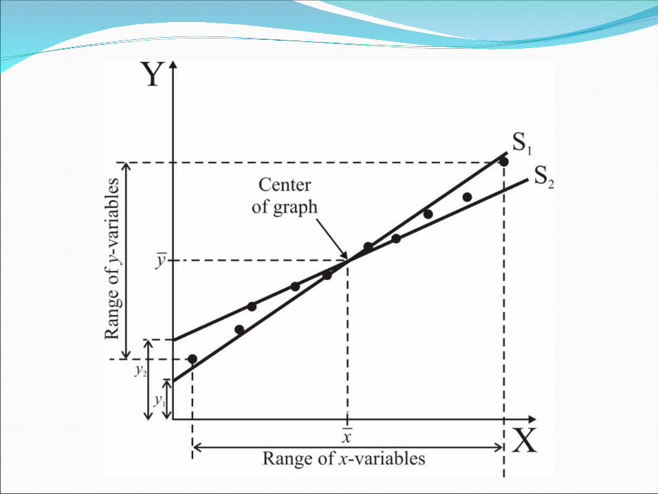
We know that the data have uncertainties. Then the position of a point on graph representing a value from data also must have the same uncertainty. The uncertainty will form a rectangular region around the marked point.

Generally, considering the uncertainty in independent variable negligible, error bars are shown for the dependent variable when all the points on the graph appear to lie on a straight line.

This is essential to determine the error in the slope.

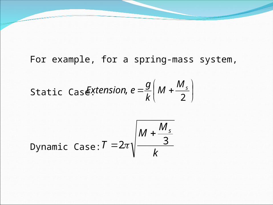
For example, for a spring-mass system,

Static Case:

Dynamic Case:

2, sMM

kgeExtension

k

MMT

s

32

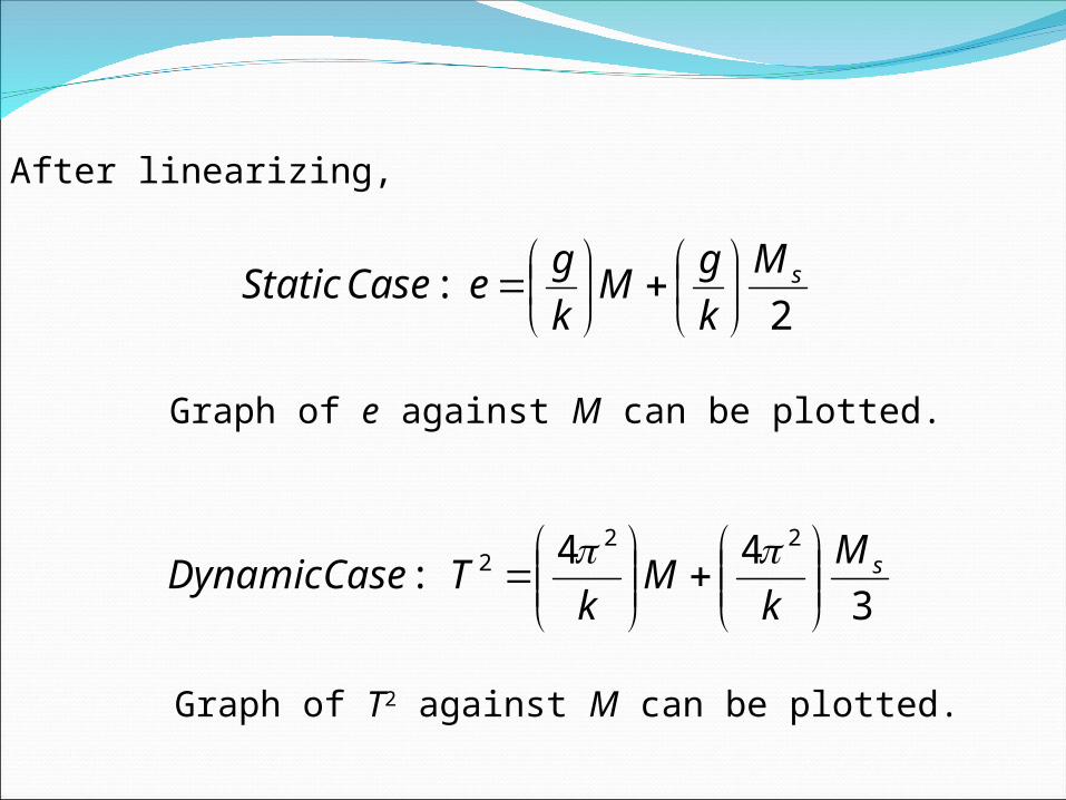
After linearizing,

2: sM

kgM

kgeCaseStatic

344:

222 sM

kM

kTCaseDynamic

Graph of e against M can be plotted.

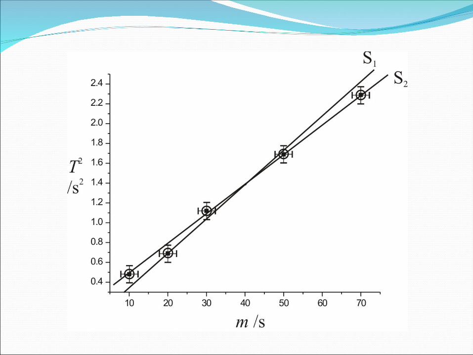
Graph of T2 against M can be plotted.

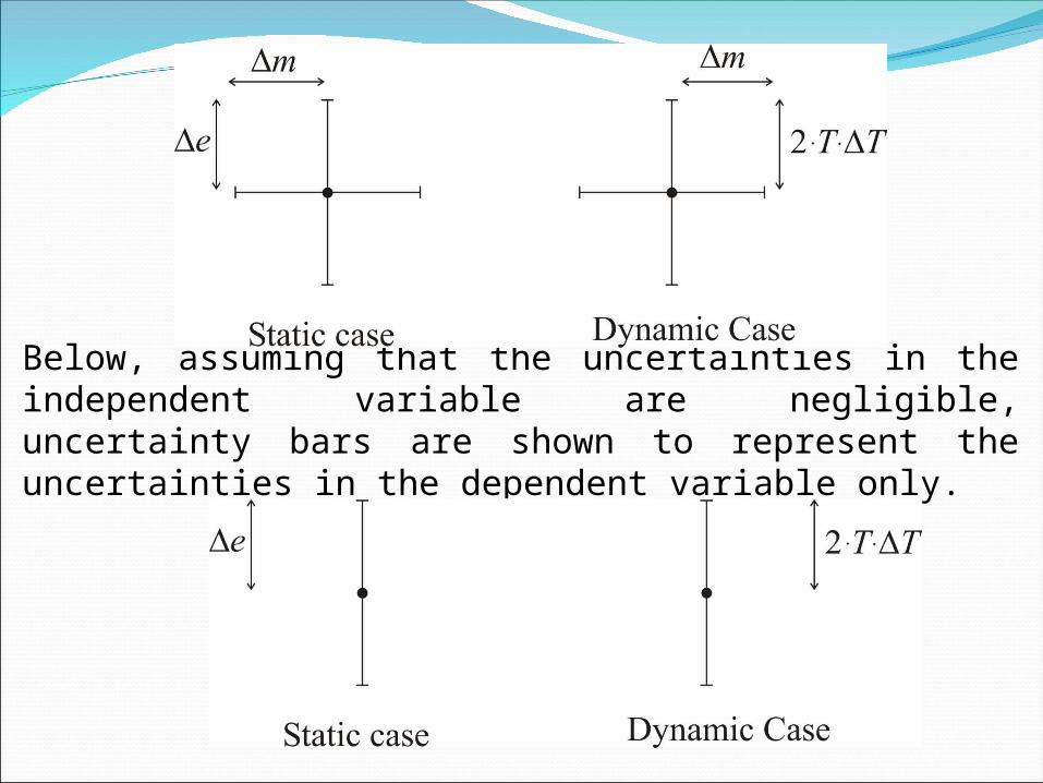
Below, assuming that the uncertainties in the independent variable are negligible, uncertainty bars are shown to represent the uncertainties in the dependent variable only.

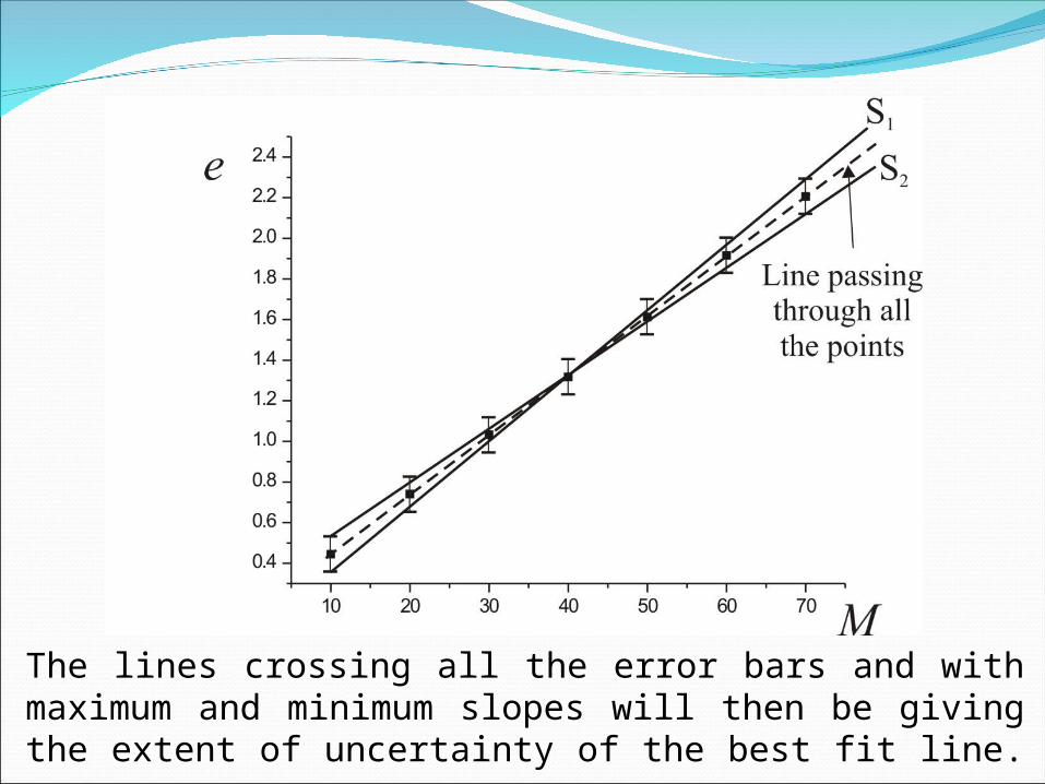
The lines crossing all the error bars and with maximum and minimum slopes will then be giving the extent of uncertainty of the best fit line.

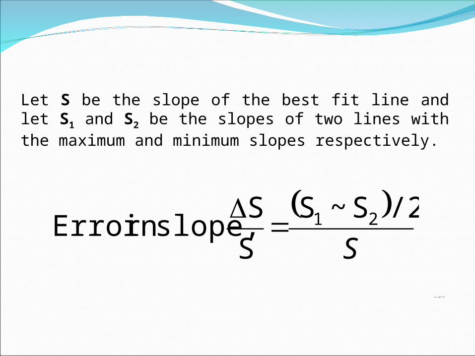
Let S be the slope of the best fit line and let S1 and S2 be the slopes of two lines with the maximum and minimum slopes respectively.

S

/2S~SSSslope,inError 21

S

/2S~SSSslope,inError 21

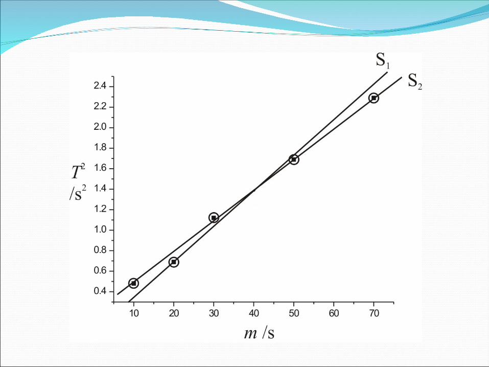
If there is large scatter and the distances of various points from the best fit are more than the length of the error bar, …

…then showing the error bars becomes useless for evaluating uncertainty in the slope because random errors (or varying systematic errors) in data are large.

Estimation of Uncertainty due to Random Errors

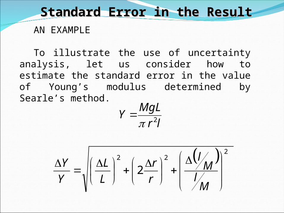
Standard Error in the ResultStandard Error in the ResultAN EXAMPLE

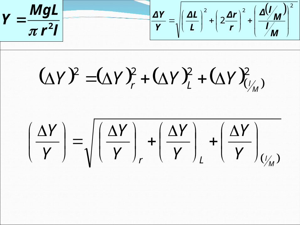
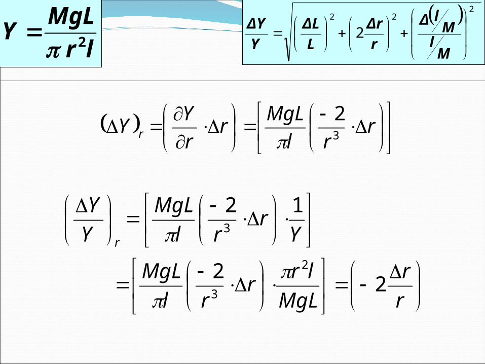
To illustrate the use of uncertainty analysis, let us consider how to estimate the standard error in the value of Young’s modulus determined by Searle’s method.

lrMgLY 2

222

2

Ml

Ml

rr

LL

YY

2222

MlYYYY Lr

MlY

YYY

YY

YY

Lr

lrMgL

Y 2

222

2

MlMlΔ

rΔr

LΔL

YΔY

rrl

MgLrrYY r 3

2

rr

MgLlrr

rlMgL

Yr

rlMgL

YY

r

22

12

2

3

3

lrMgL

Y 2

222

2

MlMlΔ

rΔr

LΔL

YΔY

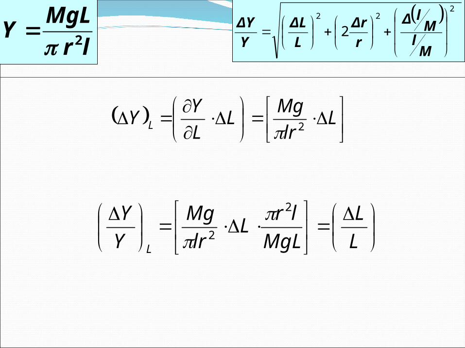
LL

MgLlrL

lrMg

YY

L

2

2

Llr

MgLLYY L 2

lrMgL

Y 2

222

2

MlMlΔ

rΔr

LΔL

YΔY

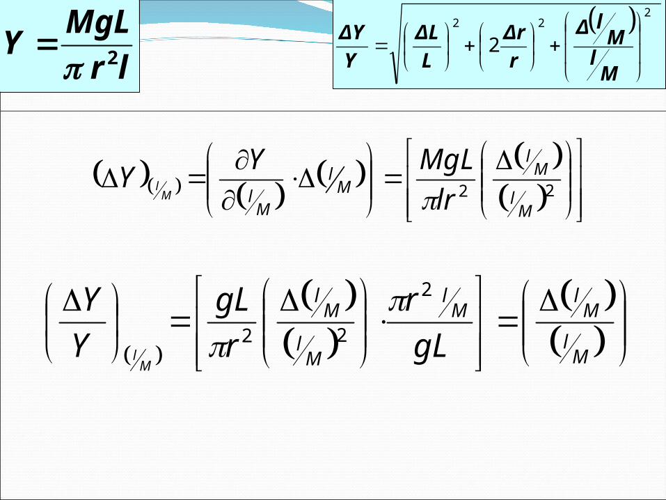
Ml

Ml

Ml

Ml

Ml

gLr

rgL

YY

Ml

2

22

22M

l

Ml

Ml

Ml lr

MgLYYM

l

lrMgL

Y 2

222

2

MlMlΔ

rΔr

LΔL

YΔY

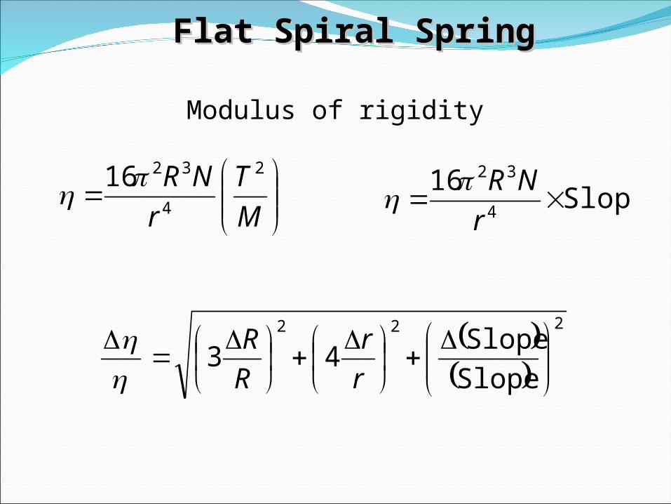
Flat Spiral SpringFlat Spiral Spring

MT

rNR 2

4

3216

Modulus of rigidity

222

SlopeSlope43

rr

RR

Slope164

32

r

NR

24

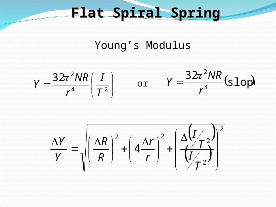
232TI

rNRY slope32

4

2

rNRY

or

Young’s Modulus

2

2

222

4

TI

TI

rr

RR

YY

Flat Spiral SpringFlat Spiral Spring

The final result should always be stated with its uncertainty.

[What in earlier textbooks was described as ‘estimation of error’ is now called evaluation of uncertainty. Error is the difference between the true value and measured value and it can never be known. What we can know is the uncertainty.]

The uncertainty is expressed only in one or two significant digits rounding the number.

Inferences and conclusions

In any measurement the uncertainty in the measured quantity is at least equal to the least count of the measuring instrument.

The final result is rounded to have the last digit at the same decimal place as the last digit in the uncertainty.

Inferences and conclusions