Doing Bayesian Data Analysis · 10/4/2012 2 Bayesian Reasoning The role of data is to re-allocate...

10/4/2012

1

Doing Bayesian Data Analysis

1© John K. Kruschke, Oct. 2012

/

| |

John K. Kruschke

© John K. Kruschke, Oct. 2012

Outline of Talk:

• Bayesian reasoning generally.

• Bayesian estimation applied to two groups. Rich information.

• The NHST t test: perfidious p values and the con game of confidence intervals.

• Conclusion: Bayesian estimation supersedes NHST.

2

10/4/2012

2

Bayesian Reasoning

The role of data is to re-allocate credibility:

Prior Credibility with New Data Posterior Credibility

via Bayes’ rule

© John K. Kruschke, Oct. 2012 3

Bayesian reasoning in everyday life is intuitive:

Sherlock Holmes: “How often have I said to you that when you have eliminated the impossible, whatever remains, however improbable, must be the truth?” (Doyle, 1890)

Judicial exoneration: For unaffiliated suspects, the incrimination of one exonerates the others.



Bayesian Reasoning

4

10/4/2012

3



1 2 3 4

Prior

Possibilities

Cre

dibi

lity

0.0

0.2

0.4

0.6

0.8

1.0

1 2 3 4

Data

Possibilities

Cre

dibi

lity

0.0

0.2

0.4

0.6

0.8

1.0

X X Xeliminate the impossible

1 2 3 4

Posterior

Possibilities

Cre

dibi

lity

0.0

0.2

0.4

0.6

0.8

1.0

whatever remainsmust be the truth




Bayesian Reasoning

5



1 2 3 4

Prior

Possibilities

Cre

dibi

lity

0.0

0.2

0.4

0.6

0.8

1.0

1 2 3 4

Data

Possibilities

Cre

dibi

lity

0.0

0.2

0.4

0.6

0.8

1.0

incrimination of one

1 2 3 4

Posterior

Possibilities

Cre

dibi

lity

0.0

0.2

0.4

0.6

0.8

1.0

X X Xexonerates the others




Credibility of the claim that the suspect

committed the crime.

Bayesian Reasoning

6

10/4/2012

4



Bayesian reasoning in data analysis is intuitive:

Possibilities are parameter values in a model, such as the mean of a normal distribution.

We reallocate credibility to parameter values that are consistent with the data.

Bayesian Data Analysis

1 2 3 4

0.0

0.2

0.4

0.6

0.8

1.0

Prior

Possibilities

Cre

dibi

lity

1 2 3 4

0.0

0.2

0.4

0.6

0.8

1.0

Data

Possibilities

Cre

dibi

lity

1 2 3 4

0.0

0.2

0.4

0.6

0.8

1.0

Posterior

Possibilities

Cre

dibi

lity

7

Bayesian Data AnalysisThe role of data is to re-allocate credibility:


1. Define a meaningful descriptive model.2. Establish prior credibility regarding parameter

values in the model. The prior credibility must be acceptable to a skeptical scientific audience.

3. Collect data.4. Use Bayes’ rule to re‐allocate credibility to

parameter values that are most consistent with the data.

8

10/4/2012

5

80 90 100 110 120 130

0.0

0.2

0.4

Data Group 1 w. Post. Pred.

y

p(y)

N1 = 47

80 90 100 110 120 130

0.0

0.2

0.4


y

p(y)

N2 = 42

Normality

log10(ν)0.0 0.2 0.4 0.6 0.8

mode = 0.247

95% HDI0.0486 0.464

Group 1 Mean

μ1100 101 102 103

mean = 102

95% HDI101 102

Group 2 Mean

μ2100 101 102 103

mean = 101

95% HDI100 101

Difference of Means

μ1 − μ2−1 0 1 2 3

mean = 1.021.1% < 0 < 98.9%

95% HDI0.17 1.89

Group 1 Std. Dev.

σ1

1 2 3 4 5

mode = 1.98

95% HDI1.28 2.95

Group 2 Std. Dev.

σ2

1 2 3 4 5

mode = 0.997

95% HDI0.672 1.47

Difference of Std. Dev.s

σ1 − σ2

0 1 2 3

mode = 0.8920.5% < 0 < 99.5%

95% HDI0.164 1.88

Effect Size

(μ1 − μ2) (σ12 + σ2

2) 2

−0.5 0.0 0.5 1.0 1.5 2.0

mode = 0.6381.1% < 0 < 98.9%

95% HDI0.0696 1.23


Robust Bayesian estimation for comparing two groups

Consider two groups; e.g., IQ of “smart drug” group and of control group.

Step 1: Define a model for describing the data.

10


Descriptive distribution for data with outliers

Normal is pulled by outliers, but tdistribution is not.

t distribution is used here as a description of data, NOT as a sampling distribution for p values!

11

10/4/2012

6


Descriptive distribution for data with outliers

The t distribution has normality controlled by the parameter .

−6 −4 −2 0 2 4 6

0.0

0.1

0.2

0.3

0.4

y

p(y)

tν=1

tν=2

tν=5normal (tν=∞)

13


The data from each group are described by tdistributions, using five parameters altogether.


14

80 90 100 110 120 130

0.00.2

0.4


y

p(y)

N1 = 47

80 90 100 110 120 130

0.00.2

0.4


y

p(y)

N2 = 42

Normality

log10(ν)0.0 0.2 0.4 0.6 0.8

mode = 0.247

95% HDI0.0486 0.464

Group 1 Mean

μ1100 101 102 103

mean = 102

95% HDI101 102

Group 2 Mean

μ2100 101 102 103

mean = 101

95% HDI100 101

Difference of Means

μ1 − μ2−1 0 1 2 3

mean = 1.021.1% < 0 < 98.9%

95% HDI0.17 1.89

Group 1 Std. Dev.

σ1

1 2 3 4 5

mode = 1.98

95% HDI1.28 2.95

Group 2 Std. Dev.

σ2

1 2 3 4 5

mode = 0.997

95% HDI0.672 1.47


σ1 − σ2

0 1 2 3

mode = 0.8920.5% < 0 < 99.5%

95% HDI0.164 1.88

Effect Size

(μ1 − μ2) (σ12 + σ2

2) 2

−0.5 0.0 0.5 1.0 1.5 2.0

mode = 0.6381.1% < 0 < 98.9%

95% HDI0.0696 1.23

80 90 100 110 120 130

0.00.2

0.4


y

p(y)

N1 = 47

80 90 100 110 120 130

0.00.2

0.4


y

p(y)

N2 = 42

Normality

log10(ν)0.0 0.2 0.4 0.6 0.8

mode = 0.247

95% HDI0.0486 0.464

Group 1 Mean

μ1100 101 102 103

mean = 102

95% HDI101 102

Group 2 Mean

μ2100 101 102 103

mean = 101

95% HDI100 101

Difference of Means

μ1 − μ2−1 0 1 2 3

mean = 1.021.1% < 0 < 98.9%

95% HDI0.17 1.89

Group 1 Std. Dev.

σ1

1 2 3 4 5

mode = 1.98

95% HDI1.28 2.95

Group 2 Std. Dev.

σ2

1 2 3 4 5

mode = 0.997

95% HDI0.672 1.47


σ1 − σ2

0 1 2 3

mode = 0.8920.5% < 0 < 99.5%

95% HDI0.164 1.88

Effect Size

(μ1 − μ2) (σ12 + σ2

2) 2

−0.5 0.0 0.5 1.0 1.5 2.0

mode = 0.6381.1% < 0 < 98.9%

95% HDI0.0696 1.23

10/4/2012

7


Step 2: Specify the prior.


15


Prior on means is wide normal.


16

10/4/2012

8


Prior on standard deviations is wide uniform.


17


Prior on normality is wide exponential.


18

10/4/2012

9


Parameter distributions will be represented by histograms: A huge number of representative parameter values.


19


Step 3: Collect Data.

80 90 100 110 120 130

0.00.2

0.4


y

p(y) N1 = 47

80 90 100 110 120 130

0.00.2

0.4


y

p(y) N2 = 42

Normality

log10(ν)0.0 0.2 0.4 0.6 0.8

mode = 0.247

95% HDI0.0486 0.464

Group 1 Mean

μ1100 101 102 103

mean = 102

95% HDI101 102

Group 2 Mean

μ2100 101 102 103

mean = 101

95% HDI100 101

Difference of Means

μ1 − μ2−1 0 1 2 3

mean = 1.021.1% < 0 < 98.9%

95% HDI0.17 1.89

Group 1 Std. Dev.

σ1

1 2 3 4 5

mode = 1.98

95% HDI1.28 2.95

Group 2 Std. Dev.

σ2

1 2 3 4 5

mode = 0.997

95% HDI0.672 1.47


σ1 − σ2

0 1 2 3

mode = 0.8920.5% < 0 < 99.5%

95% HDI0.164 1.88

Effect Size

(μ1 − μ2) (σ12 + σ2

2) 2

−0.5 0.0 0.5 1.0 1.5 2.0

mode = 0.6381.1% < 0 < 98.9%

95% HDI0.0696 1.23

80 90 100 110 120 130

0.00.2

0.4


y

p(y)

N1 = 47

80 90 100 110 120 130

0.00.2

0.4


y

p(y)

N2 = 42

Normality

log10(ν)0.0 0.2 0.4 0.6 0.8

mode = 0.247

95% HDI0.0486 0.464

Group 1 Mean

μ1100 101 102 103

mean = 102

95% HDI101 102

Group 2 Mean

μ2100 101 102 103

mean = 101

95% HDI100 101

Difference of Means

μ1 − μ2−1 0 1 2 3

mean = 1.021.1% < 0 < 98.9%

95% HDI0.17 1.89

Group 1 Std. Dev.

σ1

1 2 3 4 5

mode = 1.98

95% HDI1.28 2.95

Group 2 Std. Dev.

σ2

1 2 3 4 5

mode = 0.997

95% HDI0.672 1.47


σ1 − σ2

0 1 2 3

mode = 0.8920.5% < 0 < 99.5%

95% HDI0.164 1.88

Effect Size

(μ1 − μ2) (σ12 + σ2

2) 2

−0.5 0.0 0.5 1.0 1.5 2.0

mode = 0.6381.1% < 0 < 98.9%

95% HDI0.0696 1.23

One fixed data set, shown as red histograms.

20

10/4/2012

10


Step 4: Compute Posterior Distribution of Parameters

80 90 100 110 120 130

0.00.2

0.4


y

p(y) N1 = 47

80 90 100 110 120 130

0.00.2

0.4


y

p(y) N2 = 42

Normality

log10(ν)0.0 0.2 0.4 0.6 0.8

mode = 0.247

95% HDI0.0486 0.464

Group 1 Mean

μ1100 101 102 103

mean = 102

95% HDI101 102

Group 2 Mean

μ2100 101 102 103

mean = 101

95% HDI100 101

Difference of Means

μ1 − μ2−1 0 1 2 3

mean = 1.021.1% < 0 < 98.9%

95% HDI0.17 1.89

Group 1 Std. Dev.

σ1

1 2 3 4 5

mode = 1.98

95% HDI1.28 2.95

Group 2 Std. Dev.

σ2

1 2 3 4 5

mode = 0.997

95% HDI0.672 1.47


σ1 − σ2

0 1 2 3

mode = 0.8920.5% < 0 < 99.5%

95% HDI0.164 1.88

Effect Size

(μ1 − μ2) (σ12 + σ2

2) 2

−0.5 0.0 0.5 1.0 1.5 2.0

mode = 0.6381.1% < 0 < 98.9%

95% HDI0.0696 1.23

80 90 100 110 120 130

0.00.2

0.4


y

p(y)

N1 = 47

80 90 100 110 120 130

0.00.2

0.4


y

p(y)

N2 = 42

Normality

log10(ν)0.0 0.2 0.4 0.6 0.8

mode = 0.247

95% HDI0.0486 0.464

Group 1 Mean

μ1100 101 102 103

mean = 102

95% HDI101 102

Group 2 Mean

μ2100 101 102 103

mean = 101

95% HDI100 101

Difference of Means

μ1 − μ2−1 0 1 2 3

mean = 1.021.1% < 0 < 98.9%

95% HDI0.17 1.89

Group 1 Std. Dev.

σ1

1 2 3 4 5

mode = 1.98

95% HDI1.28 2.95

Group 2 Std. Dev.

σ2

1 2 3 4 5

mode = 0.997

95% HDI0.672 1.47


σ1 − σ2

0 1 2 3

mode = 0.8920.5% < 0 < 99.5%

95% HDI0.164 1.88

Effect Size

(μ1 − μ2) (σ12 + σ2

2) 2

−0.5 0.0 0.5 1.0 1.5 2.0

mode = 0.6381.1% < 0 < 98.9%

95% HDI0.0696 1.23

21

80 90 100 110 120 130

0.0

0.2

0.4


y

p(y)

N1 = 47

80 90 100 110 120 130

0.0

0.2

0.4


y

p(y)

N2 = 42

Normality

log10(ν)0.0 0.2 0.4 0.6 0.8

mode = 0.234

95% HDI0.0415 0.451

Group 1 Mean

μ1100 101 102 103

mean = 102

95% HDI101 102

Group 2 Mean

μ2100 101 102 103

mean = 101

95% HDI100 101

Difference of Means

μ1 − μ2−1 0 1 2 3

mean = 1.031.1% < 0 < 98.9%

95% HDI0.16 1.89

Group 1 Std. Dev.

σ1

1 2 3 4 5

mode = 1.95

95% HDI1.27 2.93

Group 2 Std. Dev.

σ2

1 2 3 4 5

mode = 0.981

95% HDI0.674 1.46


σ1 − σ2

0 1 2 3 4

mode = 0.8930.5% < 0 < 99.5%

95% HDI0.168 1.9

Effect Size

(μ1 − μ2) (σ12 + σ2

2) 2

−0.5 0.0 0.5 1.0 1.5 2.0

mode = 0.6221.1% < 0 < 98.9%

95% HDI0.0716 1.24


Step 4: Compute Posterior Distribution of Parameters

80 90 100 110 120 130

0.00.2

0.4


y

p(y) N1 = 47

80 90 100 110 120 130

0.00.2

0.4


y

p(y) N2 = 42

Normality

log10(ν)0.0 0.2 0.4 0.6 0.8

mode = 0.247

95% HDI0.0486 0.464

Group 1 Mean

μ1100 101 102 103

mean = 102

95% HDI101 102

Group 2 Mean

μ2100 101 102 103

mean = 101

95% HDI100 101

Difference of Means

μ1 − μ2−1 0 1 2 3

mean = 1.021.1% < 0 < 98.9%

95% HDI0.17 1.89

Group 1 Std. Dev.

σ1

1 2 3 4 5

mode = 1.98

95% HDI1.28 2.95

Group 2 Std. Dev.

σ2

1 2 3 4 5

mode = 0.997

95% HDI0.672 1.47


σ1 − σ2

0 1 2 3

mode = 0.8920.5% < 0 < 99.5%

95% HDI0.164 1.88

Effect Size

(μ1 − μ2) (σ12 + σ2

2) 2

−0.5 0.0 0.5 1.0 1.5 2.0

mode = 0.6381.1% < 0 < 98.9%

95% HDI0.0696 1.23

80 90 100 110 120 130

0.00.2

0.4


y

p(y)

N1 = 47

80 90 100 110 120 130

0.00.2

0.4


y

p(y)

N2 = 42

Normality

log10(ν)0.0 0.2 0.4 0.6 0.8

mode = 0.247

95% HDI0.0486 0.464

Group 1 Mean

μ1100 101 102 103

mean = 102

95% HDI101 102

Group 2 Mean

μ2100 101 102 103

mean = 101

95% HDI100 101

Difference of Means

μ1 − μ2−1 0 1 2 3

mean = 1.021.1% < 0 < 98.9%

95% HDI0.17 1.89

Group 1 Std. Dev.

σ1

1 2 3 4 5

mode = 1.98

95% HDI1.28 2.95

Group 2 Std. Dev.

σ2

1 2 3 4 5

mode = 0.997

95% HDI0.672 1.47


σ1 − σ2

0 1 2 3

mode = 0.8920.5% < 0 < 99.5%

95% HDI0.164 1.88

Effect Size

(μ1 − μ2) (σ12 + σ2

2) 2

−0.5 0.0 0.5 1.0 1.5 2.0

mode = 0.6381.1% < 0 < 98.9%

95% HDI0.0696 1.23

22

80 90 100 110 120 130

0.0

0.2

0.4


y

p(y)

N1 = 47

80 90 100 110 120 130

0.0

0.2

0.4


y

p(y)

N2 = 42

Normality

log10(ν)0.0 0.2 0.4 0.6 0.8

mode = 0.234

95% HDI0.0415 0.451

Group 1 Mean

μ1100 101 102 103

mean = 102

95% HDI101 102

Group 2 Mean

μ2100 101 102 103

mean = 101

95% HDI100 101

Difference of Means

μ1 − μ2−1 0 1 2 3

mean = 1.031.1% < 0 < 98.9%

95% HDI0.16 1.89

Group 1 Std. Dev.

σ1

1 2 3 4 5

mode = 1.95

95% HDI1.27 2.93

Group 2 Std. Dev.

σ2

1 2 3 4 5

mode = 0.981

95% HDI0.674 1.46


σ1 − σ2

0 1 2 3 4

mode = 0.8930.5% < 0 < 99.5%

95% HDI0.168 1.9

Effect Size

(μ1 − μ2) (σ12 + σ2

2) 2

−0.5 0.0 0.5 1.0 1.5 2.0

mode = 0.6221.1% < 0 < 98.9%

95% HDI0.0716 1.24

Important:These are histograms of parameter values from the posterior distribution: A huge number of combinations of that are jointly credible given the data.

These are not data distributions, and not sampling distributions from a null hypothesis.

10/4/2012

11


95% HDI:Highest density interval

Points within the HDI have higher credibility (probability density) than points outside the HDI.

The total probability of points within the 95% HDI is 95%.

Points outside the HDI may be deemed not credible.

23

80 90 100 110 120 130

0.00.2

0.4


y

p(y) N1 = 47

80 90 100 110 120 130

0.00.2

0.4


y

p(y) N2 = 42

Normality

log10(ν)0.0 0.2 0.4 0.6 0.8

mode = 0.234

95% HDI0.0415 0.451

Group 1 Mean

μ1100 101 102 103

mean = 102

95% HDI101 102

Group 2 Mean

μ2100 101 102 103

mean = 101

95% HDI100 101

Difference of Means

μ1 − μ2−1 0 1 2 3

mean = 1.031.1% < 0 < 98.9%

95% HDI0.16 1.89

Group 1 Std. Dev.

σ1

1 2 3 4 5

mode = 1.95

95% HDI1.27 2.93

Group 2 Std. Dev.

σ2

1 2 3 4 5

mode = 0.981

95% HDI0.674 1.46


σ1 − σ2

0 1 2 3 4

mode = 0.8930.5% < 0 < 99.5%

95% HDI0.168 1.9

Effect Size

(μ1 − μ2) (σ12 + σ2

2) 2

−0.5 0.0 0.5 1.0 1.5 2.0

mode = 0.6221.1% < 0 < 98.9%

95% HDI0.0716 1.24


Differences between groups?Compute and at each of the many credible combinations.

Here, both differences are credibly non‐zero.

(NHST would require two tests…)


25

80 90 100 110 120 130

0.0

0.2

0.4


y

p(y)

N1 = 47

80 90 100 110 120 130

0.0

0.2

0.4


y

p(y)

N2 = 42

Normality

log10(ν)0.0 0.2 0.4 0.6 0.8

mode = 0.234

95% HDI0.0415 0.451

Group 1 Mean

μ1100 101 102 103

mean = 102

95% HDI101 102

Group 2 Mean

μ2100 101 102 103

mean = 101

95% HDI100 101

Difference of Means

μ1 − μ2−1 0 1 2 3

mean = 1.031.1% < 0 < 98.9%

95% HDI0.16 1.89

Group 1 Std. Dev.

σ1

1 2 3 4 5

mode = 1.95

95% HDI1.27 2.93

Group 2 Std. Dev.

σ2

1 2 3 4 5

mode = 0.981

95% HDI0.674 1.46


σ1 − σ2

0 1 2 3 4

mode = 0.8930.5% < 0 < 99.5%

95% HDI0.168 1.9

Effect Size

(μ1 − μ2) (σ12 + σ2

2) 2

−0.5 0.0 0.5 1.0 1.5 2.0

mode = 0.6221.1% < 0 < 98.9%

95% HDI0.0716 1.24

10/4/2012

12


Differences between groups?Compute and at each of the many credible combinations.

Here, both differences are credibly non‐zero.

(NHST would require two tests…)


26

80 90 100 110 120 130

0.0

0.2

0.4


y

p(y)

N1 = 47

80 90 100 110 120 130

0.0

0.2

0.4


y

p(y)

N2 = 42

Normality

log10(ν)0.0 0.2 0.4 0.6 0.8

mode = 0.234

95% HDI0.0415 0.451

Group 1 Mean

μ1100 101 102 103

mean = 102

95% HDI101 102

Group 2 Mean

μ2100 101 102 103

mean = 101

95% HDI100 101

Difference of Means

μ1 − μ2−1 0 1 2 3

mean = 1.031.1% < 0 < 98.9%

95% HDI0.16 1.89

Group 1 Std. Dev.

σ1

1 2 3 4 5

mode = 1.95

95% HDI1.27 2.93

Group 2 Std. Dev.

σ2

1 2 3 4 5

mode = 0.981

95% HDI0.674 1.46


σ1 − σ2

0 1 2 3 4

mode = 0.8930.5% < 0 < 99.5%

95% HDI0.168 1.9

Effect Size

(μ1 − μ2) (σ12 + σ2

2) 2

−0.5 0.0 0.5 1.0 1.5 2.0

mode = 0.6221.1% < 0 < 98.9%

95% HDI0.0716 1.24


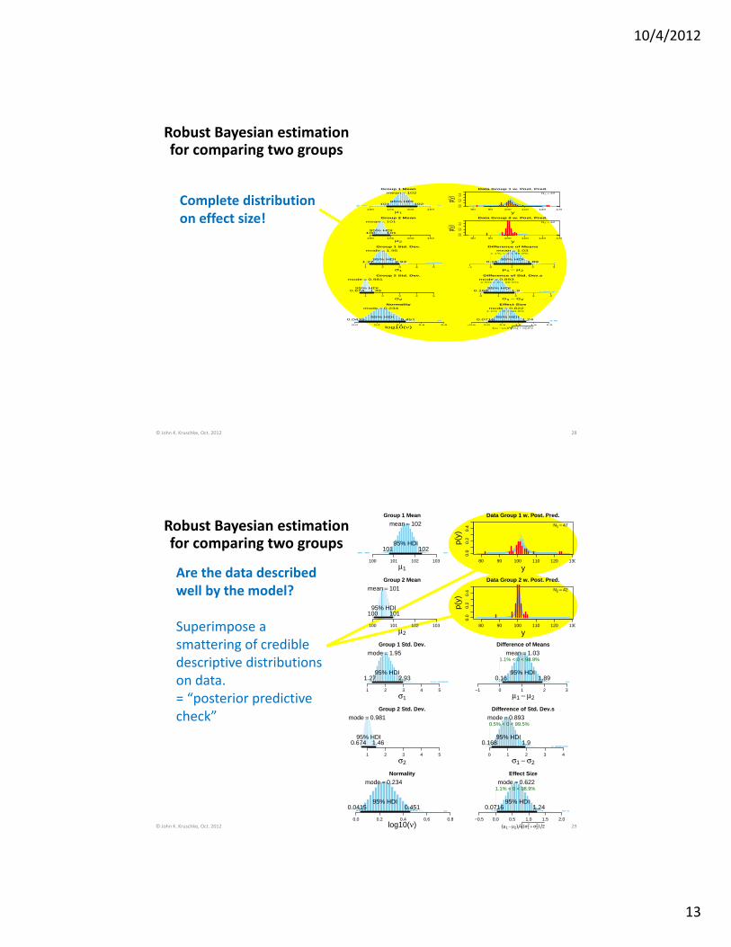
Complete distribution on effect size!


27

80 90 100 110 120 130

0.0

0.2

0.4


y

p(y)

N1 = 47

80 90 100 110 120 130

0.0

0.2

0.4


y

p(y)

N2 = 42

Normality

log10(ν)0.0 0.2 0.4 0.6 0.8

mode = 0.234

95% HDI0.0415 0.451

Group 1 Mean

μ1100 101 102 103

mean = 102

95% HDI101 102

Group 2 Mean

μ2100 101 102 103

mean = 101

95% HDI100 101

Difference of Means

μ1 − μ2−1 0 1 2 3

mean = 1.031.1% < 0 < 98.9%

95% HDI0.16 1.89

Group 1 Std. Dev.

σ1

1 2 3 4 5

mode = 1.95

95% HDI1.27 2.93

Group 2 Std. Dev.

σ2

1 2 3 4 5

mode = 0.981

95% HDI0.674 1.46


σ1 − σ2

0 1 2 3 4

mode = 0.8930.5% < 0 < 99.5%

95% HDI0.168 1.9

Effect Size

(μ1 − μ2) (σ12 + σ2

2) 2

−0.5 0.0 0.5 1.0 1.5 2.0

mode = 0.6221.1% < 0 < 98.9%

95% HDI0.0716 1.24

10/4/2012

13


Complete distribution on effect size!


28

80 90 100 110 120 130

0.00.2

0.4


y

p(y) N1 = 47

80 90 100 110 120 130

0.00.2

0.4


y

p(y) N2 = 42

Normality

log10(ν)0.0 0.2 0.4 0.6 0.8

mode = 0.234

95% HDI0.0415 0.451

Group 1 Mean

μ1100 101 102 103

mean = 102

95% HDI101 102

Group 2 Mean

μ2100 101 102 103

mean = 101

95% HDI100 101

Difference of Means

μ1 − μ2−1 0 1 2 3

mean = 1.031.1% < 0 < 98.9%

95% HDI0.16 1.89

Group 1 Std. Dev.

σ1

1 2 3 4 5

mode = 1.95

95% HDI1.27 2.93

Group 2 Std. Dev.

σ2

1 2 3 4 5

mode = 0.981

95% HDI0.674 1.46


σ1 − σ2

0 1 2 3 4

mode = 0.8930.5% < 0 < 99.5%

95% HDI0.168 1.9

Effect Size

(μ1 − μ2) (σ12 + σ2

2) 2

−0.5 0.0 0.5 1.0 1.5 2.0

mode = 0.6221.1% < 0 < 98.9%

95% HDI0.0716 1.24


Are the data described well by the model?

Superimpose a smattering of credible descriptive distributions on data.= “posterior predictive check”


29

80 90 100 110 120 130

0.0

0.2

0.4


y

p(y)

N1 = 47

80 90 100 110 120 130

0.0

0.2

0.4


y

p(y)

N2 = 42

Normality

log10(ν)0.0 0.2 0.4 0.6 0.8

mode = 0.234

95% HDI0.0415 0.451

Group 1 Mean

μ1100 101 102 103

mean = 102

95% HDI101 102

Group 2 Mean

μ2100 101 102 103

mean = 101

95% HDI100 101

Difference of Means

μ1 − μ2−1 0 1 2 3

mean = 1.031.1% < 0 < 98.9%

95% HDI0.16 1.89

Group 1 Std. Dev.

σ1

1 2 3 4 5

mode = 1.95

95% HDI1.27 2.93

Group 2 Std. Dev.

σ2

1 2 3 4 5

mode = 0.981

95% HDI0.674 1.46


σ1 − σ2

0 1 2 3 4

mode = 0.8930.5% < 0 < 99.5%

95% HDI0.168 1.9

Effect Size

(μ1 − μ2) (σ12 + σ2

2) 2

−0.5 0.0 0.5 1.0 1.5 2.0

mode = 0.6221.1% < 0 < 98.9%

95% HDI0.0716 1.24

10/4/2012

14


Are the data described well by the model?

Superimpose a smattering of credible descriptive distributions on data.= “posterior predictive check”


80 90 100 110 120 130

0.0

0.2

0.4


y

p(y)

N1 = 47

80 90 100 110 120 130

0.0

0.2

0.4


y

p(y)

N2 = 42

Normality

log10(ν)0.0 0.2 0.4 0.6 0.8

mode = 0.247

95% HDI0.0486 0.464

Group 1 Mean

μ1100 101 102 103

mean = 102

95% HDI101 102

Group 2 Mean

μ2100 101 102 103

mean = 101

95% HDI100 101

Difference of Means

μ1 − μ2−1 0 1 2 3

mean = 1.021.1% < 0 < 98.9%

95% HDI0.17 1.89

Group 1 Std. Dev.

σ1

1 2 3 4 5

mode = 1.98

95% HDI1.28 2.95

Group 2 Std. Dev.

σ2

1 2 3 4 5

mode = 0.997

95% HDI0.672 1.47


σ1 − σ2

0 1 2 3

mode = 0.8920.5% < 0 < 99.5%

95% HDI0.164 1.88

Effect Size

(μ1 − μ2) (σ12 + σ2

2) 2

−0.5 0.0 0.5 1.0 1.5 2.0

mode = 0.6381.1% < 0 < 98.9%

95% HDI0.0696 1.23

30


Summary: Complete distribution of credible parameter values (not merely point estimate with ends of confidence interval). Decisions about multiple aspects of parameters (without reference to p values). Flexible descriptive model, robust to outliers (unlike NHST t test).


31

80 90 100 110 120 130

0.0

0.2

0.4


y

p(y)

N1 = 47

80 90 100 110 120 130

0.0

0.2

0.4


y

p(y)

N2 = 42

Normality

log10(ν)0.0 0.2 0.4 0.6 0.8

mode = 0.234

95% HDI0.0415 0.451

Group 1 Mean

μ1100 101 102 103

mean = 102

95% HDI101 102

Group 2 Mean

μ2100 101 102 103

mean = 101

95% HDI100 101

Difference of Means

μ1 − μ2−1 0 1 2 3

mean = 1.031.1% < 0 < 98.9%

95% HDI0.16 1.89

Group 1 Std. Dev.

σ1

1 2 3 4 5

mode = 1.95

95% HDI1.27 2.93

Group 2 Std. Dev.

σ2

1 2 3 4 5

mode = 0.981

95% HDI0.674 1.46


σ1 − σ2

0 1 2 3 4

mode = 0.8930.5% < 0 < 99.5%

95% HDI0.168 1.9

Effect Size

(μ1 − μ2) (σ12 + σ2

2) 2

−0.5 0.0 0.5 1.0 1.5 2.0

mode = 0.6221.1% < 0 < 98.9%

95% HDI0.0716 1.24

10/4/2012

15


source("BEST.R") # load the program

# Specify data as vectors (replace with your own data):y1 = c(101,100,102,104,102,97,105,105,98,101,100,123,105,

109,102,82,102,100,102,102,101,102,102,103,103,97,96,103,124,101,101,100,101,101,104,100,101)

y2 = c(99,101,100,101,102,100,97,101,104,101,102,102,100,104,100,100,100,101,102,103,97,101,101,100,101,99,101,100,99,101,100,102,99,100,99)

# Run the Bayesian analysis:mcmcChain = BESTmcmc( y1 , y2 )

# Plot the results of the Bayesian analysis:BESTplot( y1 , y2 , mcmcChain )

Computer Software:

Packaged for easy use! Underlying program is never seen.

© John K. Kruschke, Sept. 2012


Download the programs from http://www.indiana.edu/~kruschke/BEST/BEST.zip

33

Now for a look under the hood

http://www.autonationconnect.com/2010/07/backseat‐mechanic‐under‐the‐hoo/

10/4/2012

16

© John K. Kruschke, Sept. 2012 34

Doing it with JAGS

R programming language

JAGS executables

“JAGS” = Just Another Gibbs Samplerbut other sampling methods are incorporated.

rjagscommands

JAGS makes it easy. You specify only the• prior function • likelihood functionand JAGS does the rest! You do no math, no selection of sampling methods.


JAGS and BUGS

10/4/2012

17


Installation: See Blog Entryhttp://doingbayesiandataanalysis.blogspot.com/2012/01/complete‐steps‐for‐installing‐software.html


Robust Bayesian estimation for comparing two groups model {

for ( i in 1:Ntotal ) {y[i] ~ dt( mu[x[i]] , tau[x[i]] , nu )

}for ( j in 1:2 ) {mu[j] ~ dnorm( muM , muP )tau[j] <- 1/pow( sigma[j] , 2 )sigma[j] ~ dunif( sigmaLow , sigmaHigh )

}nu <- nuMinusOne+1nuMinusOne ~ dexp(1/29)

}

Program BEST.R: JAGS model specification.

37

10/4/2012

18



38

model {for ( i in 1:Ntotal ) {y[i] ~ dt( mu[x[i]] , tau[x[i]] , nu )



}




Nested indexing: x[i] is the group (1 or 2)

of the ith score.

39




}


10/4/2012

19



40




}




41




}


10/4/2012

20



42




}


Five main sections in all programs:

1. Specify model (we just did this).

2. Load data.

3. Initialize the MCMC chain.

4. Run the MCMC chain.

5. Examine the results.


Programs in R + rjags + JAGS:

10/4/2012

21


BEST.RBESTmcmc = function( y1, y2, numSavedSteps=100000, thinSteps=1, showMCMC=FALSE) { # This function generates an MCMC sample from the posterior distribution.# Description of arguments:# showMCMC is a flag for displaying diagnostic graphs of the chains.# If F (the default), no chain graphs are displayed. If T, they are.

require(rjags)

#------------------------------------------------------------------------------# THE MODEL.modelString = "model {for ( i in 1:Ntotal ) {y[i] ~ dt( mu[x[i]] , tau[x[i]] , nu )



}" # close quote for modelString# Write out modelString to a text filewriteLines( modelString , con="BESTmodel.txt" )

#------------------------------------------------------------------------------# THE DATA.# Load the data:y = c( y1 , y2 ) # combine data into one vectorx = c( rep(1,length(y1)) , rep(2,length(y2)) ) # create group membership codeNtotal = length(y)# Specify the data in a list, for later shipment to JAGS:dataList = list(y = y ,x = x ,Ntotal = Ntotal ,


BEST.RBESTmcmc = function( y1, y2, numSavedSteps=100000, thinSteps=1, showMCMC=FALSE) { # This function generates an MCMC sample from the posterior distribution.# Description of arguments:# showMCMC is a flag for displaying diagnostic graphs of the chains.# If F (the default), no chain graphs are displayed. If T, they are.

require(rjags)

#------------------------------------------------------------------------------# THE MODEL.modelString = "model {for ( i in 1:Ntotal ) {y[i] ~ dt( mu[x[i]] , tau[x[i]] , nu )




#------------------------------------------------------------------------------# THE DATA.# Load the data:y = c( y1 , y2 ) # combine data into one vectorx = c( rep(1,length(y1)) , rep(2,length(y2)) ) # create group membership codeNtotal = length(y)# Specify the data in a list, for later shipment to JAGS:dataList = list(y = y ,x = x ,Ntotal = Ntotal ,

10/4/2012

22


BEST.R

g [j] ( g , g g )}nu <- nuMinusOne+1nuMinusOne ~ dexp(1/29)


#------------------------------------------------------------------------------# THE DATA.# Load the data:y = c( y1 , y2 ) # combine data into one vectorx = c( rep(1,length(y1)) , rep(2,length(y2)) ) # create group membership codeNtotal = length(y)# Specify the data in a list, for later shipment to JAGS:dataList = list(y = y ,x = x ,Ntotal = Ntotal ,muM = mean(y) ,muP = 0.000001 * 1/sd(y)^2 ,sigmaLow = sd(y) / 1000 ,sigmaHigh = sd(y) * 1000

)

#------------------------------------------------------------------------------# INTIALIZE THE CHAINS.# Initial values of MCMC chains based on data:mu = c( mean(y1) , mean(y2) )sigma = c( sd(y1) , sd(y2) )# Regarding initial values in next line: (1) sigma will tend to be too big if # the data have outliers, and (2) nu starts at 5 as a moderate value. These# initial values keep the burn-in period moderate.initsList = list( mu = mu , sigma = sigma , nuMinusOne = 4 )

#------------------------------------------------------------------------------# RUN THE CHAINS

parameters = c( "mu" , "sigma" , "nu" ) # The parameters to be monitoredadaptSteps = 500 # Number of steps to "tune" the samplersburnInSteps = 1000nChains = 3 nIter = ceiling( ( numSavedSteps * thinSteps ) / nChains )


BEST.R

g [j] ( g , g g )}nu <- nuMinusOne+1nuMinusOne ~ dexp(1/29)


#------------------------------------------------------------------------------# THE DATA.# Load the data:y = c( y1 , y2 ) # combine data into one vectorx = c( rep(1,length(y1)) , rep(2,length(y2)) ) # create group membership codeNtotal = length(y)# Specify the data in a list, for later shipment to JAGS:dataList = list(y = y ,x = x ,Ntotal = Ntotal ,muM = mean(y) ,muP = 0.000001 * 1/sd(y)^2 ,sigmaLow = sd(y) / 1000 ,sigmaHigh = sd(y) * 1000

)

#------------------------------------------------------------------------------# INTIALIZE THE CHAINS.# Initial values of MCMC chains based on data:mu = c( mean(y1) , mean(y2) )sigma = c( sd(y1) , sd(y2) )# Regarding initial values in next line: (1) sigma will tend to be too big if # the data have outliers, and (2) nu starts at 5 as a moderate value. These# initial values keep the burn-in period moderate.initsList = list( mu = mu , sigma = sigma , nuMinusOne = 4 )

#------------------------------------------------------------------------------# RUN THE CHAINS

parameters = c( "mu" , "sigma" , "nu" ) # The parameters to be monitoredadaptSteps = 500 # Number of steps to "tune" the samplersburnInSteps = 1000nChains = 3 nIter = ceiling( ( numSavedSteps * thinSteps ) / nChains )

10/4/2012

23


BEST.R# initial values keep the burn-in period moderate.initsList = list( mu = mu , sigma = sigma , nuMinusOne = 4 )

#------------------------------------------------------------------------------# RUN THE CHAINS

parameters = c( "mu" , "sigma" , "nu" ) # The parameters to be monitoredadaptSteps = 500 # Number of steps to "tune" the samplersburnInSteps = 1000nChains = 3 nIter = ceiling( ( numSavedSteps * thinSteps ) / nChains )# Create, initialize, and adapt the model:jagsModel = jags.model( "BESTmodel.txt" , data=dataList , inits=initsList ,

n.chains=nChains , n.adapt=adaptSteps )# Burn-in:cat( "Burning in the MCMC chain...\n" )update( jagsModel , n.iter=burnInSteps )# The saved MCMC chain:cat( "Sampling final MCMC chain...\n" )codaSamples = coda.samples( jagsModel , variable.names=parameters ,

n.iter=nIter , thin=thinSteps )# resulting codaSamples object has these indices: # codaSamples[[ chainIdx ]][ stepIdx , paramIdx ]

#------------------------------------------------------------------------------# EXAMINE THE RESULTSif ( showMCMC ) {windows()autocorr.plot( codaSamples[[1]] , ask=FALSE )

}

# Convert coda-object codaSamples to matrix object for easier handling.# But note that this concatenates the different chains into one long chain.# Result is mcmcChain[ stepIdx , paramIdx ]mcmcChain = as.matrix( codaSamples )return( mcmcChain )

} # end function BESTmcmc


BEST.R# initial values keep the burn-in period moderate.initsList = list( mu = mu , sigma = sigma , nuMinusOne = 4 )

#------------------------------------------------------------------------------# RUN THE CHAINS

parameters = c( "mu" , "sigma" , "nu" ) # The parameters to be monitoredadaptSteps = 500 # Number of steps to "tune" the samplersburnInSteps = 1000nChains = 3 nIter = ceiling( ( numSavedSteps * thinSteps ) / nChains )# Create, initialize, and adapt the model:jagsModel = jags.model( "BESTmodel.txt" , data=dataList , inits=initsList ,

n.chains=nChains , n.adapt=adaptSteps )# Burn-in:cat( "Burning in the MCMC chain...\n" )update( jagsModel , n.iter=burnInSteps )# The saved MCMC chain:cat( "Sampling final MCMC chain...\n" )codaSamples = coda.samples( jagsModel , variable.names=parameters ,

n.iter=nIter , thin=thinSteps )# resulting codaSamples object has these indices: # codaSamples[[ chainIdx ]][ stepIdx , paramIdx ]

#------------------------------------------------------------------------------# EXAMINE THE RESULTSif ( showMCMC ) {windows()autocorr.plot( codaSamples[[1]] , ask=FALSE )

}

# Convert coda-object codaSamples to matrix object for easier handling.# But note that this concatenates the different chains into one long chain.# Result is mcmcChain[ stepIdx , paramIdx ]mcmcChain = as.matrix( codaSamples )return( mcmcChain )

} # end function BESTmcmc

10/4/2012

24


source("BEST.R") # load the program

# Specify data as vectors (replace with your own data):y1 = c(101,100,102,104,102,97,105,105,98,101,100,123,105,

109,102,82,102,100,102,102,101,102,102,103,103,97,96,103,124,101,101,100,101,101,104,100,101)

y2 = c(99,101,100,101,102,100,97,101,104,101,102,102,100,104,100,100,100,101,102,103,97,101,101,100,101,99,101,100,99,101,100,102,99,100,99)

# Run the Bayesian analysis:mcmcChain = BESTmcmc( y1 , y2 )

# Plot the results of the Bayesian analysis:BESTplot( y1 , y2 , mcmcChain )

Computer Software:

Packaged for easy use! Underlying program is never seen.


Summary: Complete distribution of credible parameter values (not merely point estimate with ends of confidence interval). Decisions about multiple aspects of parameters (without reference to p values). Flexible descriptive model, robust to outliers (unlike NHST t test).

Recall Bayesian estimation for comparing two groups

51

80 90 100 110 120 130

0.0

0.2

0.4


y

p(y)

N1 = 47

80 90 100 110 120 130

0.0

0.2

0.4


y

p(y)

N2 = 42

Normality

log10(ν)0.0 0.2 0.4 0.6 0.8

mode = 0.234

95% HDI0.0415 0.451

Group 1 Mean

μ1100 101 102 103

mean = 102

95% HDI101 102

Group 2 Mean

μ2100 101 102 103

mean = 101

95% HDI100 101

Difference of Means

μ1 − μ2−1 0 1 2 3

mean = 1.031.1% < 0 < 98.9%

95% HDI0.16 1.89

Group 1 Std. Dev.

σ1

1 2 3 4 5

mode = 1.95

95% HDI1.27 2.93

Group 2 Std. Dev.

σ2

1 2 3 4 5

mode = 0.981

95% HDI0.674 1.46


σ1 − σ2

0 1 2 3 4

mode = 0.8930.5% < 0 < 99.5%

95% HDI0.168 1.9

Effect Size

(μ1 − μ2) (σ12 + σ2

2) 2

−0.5 0.0 0.5 1.0 1.5 2.0

mode = 0.6221.1% < 0 < 98.9%

95% HDI0.0716 1.24

10/4/2012

25

80 90 100 110 120 130

0.0

0.2

0.4


y

p(y)

N1 = 47

80 90 100 110 120 130

0.0

0.2

0.4


y

p(y)

N2 = 42

Normality

log10(ν)0.0 0.2 0.4 0.6 0.8

mode = 0.234

95% HDI0.0415 0.451

Group 1 Mean

μ1100 101 102 103

mean = 102

95% HDI101 102

Group 2 Mean

μ2100 101 102 103

mean = 101

95% HDI100 101

Difference of Means

μ1 − μ2−1 0 1 2 3

mean = 1.031.1% < 0 < 98.9%

95% HDI0.16 1.89

Group 1 Std. Dev.

σ1

1 2 3 4 5

mode = 1.95

95% HDI1.27 2.93

Group 2 Std. Dev.

σ2

1 2 3 4 5

mode = 0.981

95% HDI0.674 1.46


σ1 − σ2

0 1 2 3 4

mode = 0.8930.5% < 0 < 99.5%

95% HDI0.168 1.9

Effect Size

(μ1 − μ2) (σ12 + σ2

2) 2

−0.5 0.0 0.5 1.0 1.5 2.0

mode = 0.6221.1% < 0 < 98.9%

95% HDI0.0716 1.24


What does NHST say?

t test of means: t(87)=1.62, p=0.110 (>.05)95%CI: ‐0.361 to 3.477.

F test of variances:F(46,41)=5.72, p < .001.95%CI on difference: ?

But,must apply corrections for multiple tests.

Recall Bayesian estimation:

52

80 90 100 110 120 130

0.0

0.2

0.4


y

p(y)

N1 = 47

80 90 100 110 120 130

0.0

0.2

0.4


y

p(y)

N2 = 42

Normality

log10(ν)0.0 0.2 0.4 0.6 0.8

mode = 0.234

95% HDI0.0415 0.451

Group 1 Mean

μ1100 101 102 103

mean = 102

95% HDI101 102

Group 2 Mean

μ2100 101 102 103

mean = 101

95% HDI100 101

Difference of Means

μ1 − μ2−1 0 1 2 3

mean = 1.031.1% < 0 < 98.9%

95% HDI0.16 1.89

Group 1 Std. Dev.

σ1

1 2 3 4 5

mode = 1.95

95% HDI1.27 2.93

Group 2 Std. Dev.

σ2

1 2 3 4 5

mode = 0.981

95% HDI0.674 1.46


σ1 − σ2

0 1 2 3 4

mode = 0.8930.5% < 0 < 99.5%

95% HDI0.168 1.9

Effect Size

(μ1 − μ2) (σ12 + σ2

2) 2

−0.5 0.0 0.5 1.0 1.5 2.0

mode = 0.6221.1% < 0 < 98.9%

95% HDI0.0716 1.24


What does NHST say?Oops! Data are not normal, so do resampling instead.

Resampling test of means: p=0.116 (>.05)

Resampling test of difference of standard deviations:p = 0.072 (>.05)

And, still must apply corrections for multiple tests.And there are no CI’s.

Recall Bayesian estimation:

53

10/4/2012

26


Example with outliers: BESTexample.R

Bayesian estimation:• Credible differences between means

and standard deviations.• Complete distributional information

on effect size and everything else.• Non‐normality indicated.

NHST t test:• Outliers invalidate classic test.• Resampling shows p>.05 for difference

of means, p>.05 for difference of standard deviations.

• Need correction for multiple tests.• No CI’s. (And CI’s would have no

distributional info and fickle end points linked to fickle p values.)

80 90 100 110 120 130

0.0

0.2

0.4


y

p(y)

N1 = 47

80 90 100 110 120 130

0.0

0.2

0.4


y

p(y)

N2 = 42

Normality

log10(ν)0.0 0.2 0.4 0.6 0.8

mode = 0.234

95% HDI0.0415 0.451

Group 1 Mean

μ1100 101 102 103

mean = 102

95% HDI101 102

Group 2 Mean

μ2100 101 102 103

mean = 101

95% HDI100 101

Difference of Means

μ1 − μ2−1 0 1 2 3

mean = 1.031.1% < 0 < 98.9%

95% HDI0.16 1.89

Group 1 Std. Dev.

σ1

1 2 3 4 5

mode = 1.95

95% HDI1.27 2.93

Group 2 Std. Dev.

σ2

1 2 3 4 5

mode = 0.981

95% HDI0.674 1.46


σ1 − σ2

0 1 2 3 4

mode = 0.8930.5% < 0 < 99.5%

95% HDI0.168 1.9

Effect Size

(μ1 − μ2) (σ12 + σ2

2) 2

−0.5 0.0 0.5 1.0 1.5 2.0

mode = 0.6221.1% < 0 < 98.9%

95% HDI0.0716 1.24


Example with small NBayesian estimation:• Zero is among credible differences

between means and standard deviations, and for effect size.

• Complete distributional information on effect size and everything else.

• Normality is credible.

NHST t test:• t(14)=2.33, p=0.035, 95% CI: 0.099,

2.399. (F(7,7)=1.00, p=.999, CI on ratio: 0.20, 5.00.)

• Need correction for multiple tests, if intended.

• CI’s have no distributional info and fickle end points linked to fickle pvalues.

• t test fails to reveal true uncertainty in parameter estimates when simultaneously estimating SD’s and normality.

−1 0 1 2 3

0.0

0.3

0.6


y

p(y)

N1 = 8

−1 0 1 2 3

0.0

0.3

0.6


y

p(y)

N2 = 8

Normality

log10(ν)0.0 0.5 1.0 1.5 2.0 2.5

mode = 1.45

95% HDI0.595 2.09

Group 1 Mean

μ1−4 −2 0 2 4

mean = 1.25

95% HDI0.24 2.2

Group 2 Mean

μ2−4 −2 0 2 4

mean = −0.0124

95% HDI−1.01 0.982

Difference of Means

μ1 − μ2−4 −2 0 2 4

mean = 1.263.6% < 0 < 96.4%

95% HDI−0.111 2.67

Group 1 Std. Dev.

σ1

0 2 4 6 8

mode = 1.06

95% HDI0.581 2.21

Group 2 Std. Dev.

σ2

0 2 4 6 8

mode = 1.04

95% HDI0.597 2.24


σ1 − σ2

−6 −4 −2 0 2 4 6

mode = −0.011750.7% < 0 < 49.3%

95% HDI−1.37 1.37

Effect Size

(μ1 − μ2) (σ12 + σ2

2) 2

−1 0 1 2 3 4

mode = 1.033.6% < 0 < 96.4%

95% HDI−0.104 2.17

10/4/2012

27


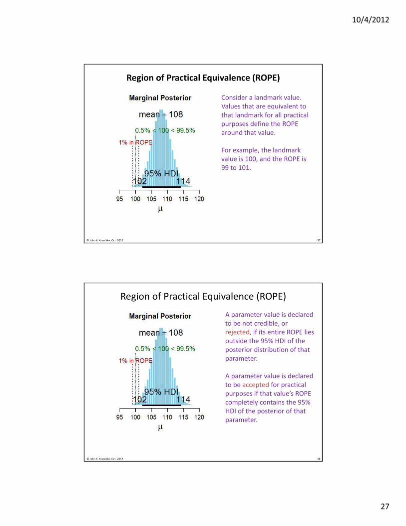
Region of Practical Equivalence (ROPE)

Consider a landmark value. Values that are equivalent to that landmark for all practical purposes define the ROPE around that value.

For example, the landmark value is 100, and the ROPE is 99 to 101.


Region of Practical Equivalence (ROPE)

A parameter value is declared to be not credible, or rejected, if its entire ROPE lies outside the 95% HDI of the posterior distribution of that parameter.

A parameter value is declared to be accepted for practical purposes if that value’s ROPE completely contains the 95% HDI of the posterior of that parameter.

10/4/2012

28


Example of accepting null value

Bayesian estimation:• 95% HDI for difference on means falls

within ROPE; same for SD’s (enlarged in next slide).

• Complete distributional information on effect size and everything else.

• Normality is credible.

NHST t test:• p is large for both t and F tests, but

NHST cannot accept null hypothesis.• Need correction for multiple tests, if

intended.• CI’s have no distributional info and

fickle end points linked to fickle pvalues, and CI does not indicate probability of parameter value. Hence, cannot use ROPE method in NHST.

−4 −2 0 2 4

0.0

0.2

0.4


y

p(y)

N1 = 1101

−4 −2 0 2 4

0.0

0.2

0.4


y

p(y)

N2 = 1090

Normality

log10(ν)1.0 1.5 2.0 2.5

mode = 1.66

95% HDI1.3 2.1

Group 1 Mean

μ1−0.10 −0.05 0.00 0.05 0.10

mean = −0.000297

95% HDI−0.0612 0.058

Group 2 Mean

μ2−0.10 −0.05 0.00 0.05 0.10

mean = 0.00128

95% HDI−0.0579 0.0609

Difference of Means

μ1 − μ2−0.2 −0.1 0.0 0.1 0.2

mean = −0.0015851.6% < 0 < 48.4%

98% in ROPE

95% HDI−0.084 0.0832

Group 1 Std. Dev.

σ1

0.90 0.95 1.00 1.05

mode = 0.986

95% HDI0.939 1.03

Group 2 Std. Dev.

σ2

0.90 0.95 1.00 1.05

mode = 0.985

95% HDI0.938 1.03


σ1 − σ2

−0.10 −0.05 0.00 0.05 0.10

mode = 0.00015450% < 0 < 50%100% in ROPE

95% HDI−0.0608 0.0598

Effect Size

(μ1 − μ2) (σ12 + σ2

2) 2

−0.2 −0.1 0.0 0.1 0.2

mode = −0.0034251.6% < 0 < 48.4%

95% HDI−0.0861 0.0837


Example of accepting null value

Bayesian estimation:• 95% HDI for difference on means falls

within ROPE; same for SD’s.• Complete distributional information

on effect size and everything else.• Normality is credible.

NHST t test:• p is large for both t and F tests, but

NHST cannot accept null hypothesis.• Need correction for multiple tests, if

intended.• CI’s have no distributional info and

fickle end points linked to fickle pvalues, and CI does not indicate probability of parameter value. Hence, cannot use ROPE method in NHST.

−4 −2 0 2 4

0.0

0.2

0.4


y

p(y

)

N1 = 1101

−4 −2 0 2 4

0.0

0.2

0.4


y

p(y

)

N2 = 1090

Normality

log10(ν)1.0 1.5 2.0 2.5

mode = 1.66

95% HDI1.3 2.1

Group 1 Mean

μ1−0.10 −0.05 0.00 0.05 0.10

mean = −0.000297

95% HDI−0.0612 0.058

Group 2 Mean

μ2−0.10 −0.05 0.00 0.05 0.10

mean = 0.00128

95% HDI−0.0579 0.0609

Difference of Means

μ1 − μ2−0.2 −0.1 0.0 0.1 0.2

mean = −0.0015851.6% < 0 < 48.4%

98% in ROPE

95% HDI−0.084 0.0832

Group 1 Std. Dev.

σ1

0.90 0.95 1.00 1.05

mode = 0.986

95% HDI0.939 1.03

Group 2 Std. Dev.

σ2

0.90 0.95 1.00 1.05

mode = 0.985

95% HDI0.938 1.03


σ1 − σ2

−0.10 −0.05 0.00 0.05 0.10

mode = 0.00015450% < 0 < 50%100% in ROPE

95% HDI−0.0608 0.0598

Effect Size

(μ1 − μ2) (σ12 + σ2

2) 2

−0.2 −0.1 0.0 0.1 0.2

mode = −0.0034251.6% < 0 < 48.4%

95% HDI−0.0861 0.0837

10/4/2012

29


Sequential TestingFor simulated data from the null hypothesis:


Sequential TestingFor simulated data from the null hypothesis:

10/4/2012

30


Many other topics are in the book, e.g.

Bayesian hierarchical ANOVA, oneway and twowaywith interaction contrasts. The generalized linear model. Many types of regression, including multiple linear regression, logistic regression, ordinal regression. Log‐linear models vs chi‐square test. Power: Probability of achieving the goals of research. All preceded by extensive introductory chapterscovering notions of probability, Bayes’ rule, MCMC, model comparison, etc.

An example of a t test:Data:Group 1: 5.70 5.40 5.75 5.25 4.25 4.74; M1 = 5.18Group 2: 4.55 4.98 4.70 4.78 3.26 3.67; M2 = 4.32

t = 2.33

Show of hands please:

Who bets that p < .05 ? Who bets that p > .05 ?


10/4/2012

31


t = 2.33

Show of hands please:

Who bets that p < .05 ? Who bets that p > .05 ?

You’re right! You’re right!


Null Hypothesis Significance Testing (NHST)

Consider how we draw conclusions from data:

• Collect data, carefully insulated from our intentions.

Double blind clinical designs.

No datum is influenced by any other datum before or after.

• Compute a summary statistic, e.g., for a difference between groups, the t statistic.

• Compute p value of t. If p < .05, declare the result to be “significant.”


10/4/2012

32

Null Hypothesis Significance Testing (NHST)

Consider how we draw conclusions from data:

• Collect data, carefully insulated from our intentions.

Double blind clinical designs

No datum is influenced by any other datum before or after.

• Compute a summary statistic, e.g., for a difference between groups, the t statistic.

• Compute p value of t. If p < .05, declare the result to be “significant.”

Value of p depends on the intention of the experimenter!


The road to NHST is paved with good intentions.

The p value is the probability that the actual sample statistic, or a result more extreme, would be obtained from the null hypothesis, if the intended experiment were repeated ad infinitum.


value null act for null sampled according to

the intended experiment

68

10/4/2012

33

Space of possible outcomesfrom null hypothesis


“The” p value…

p value Actual

outcome

∅

69



p value for intention to sample until N

p value Actual

outcome

NNNNNNN

70

10/4/2012

34



p value Actual

outcome

TTTTTT

p value for intention to sample until Time

71


The distribution of twhen the intended experiment is repeated many times

y0

y0

Null Hypothesis:Groups are identical

Many simulated repetitions of the

intendedexperiment


NN

73

10/4/2012

35

The distribution of twhen the intended experiment is repeated many times

y0

y0



intendedexperiment



The intention to collect data until the end of the week

y0

y0



intendedexperiment


T

75

10/4/2012

36

The intention to collect data until the end of the week

y0

y0



intendedexperiment



t = 2.33

Can the null hypothesis be rejected? To answer, we must know the intention of the data collector.• We ask the research assistant who collected the data. The assistant says, “I just collected data for two weeks. It’s my job. I happened to get 6 subjects in each group.” • We ask the graduate student who oversaw the assistant. The student says, “I knew we needed 6 subjects per group, so I told the assistant to run for two weeks, because we usually get about 6 subjects per week.” • We ask the lab director, who says, “I told my graduate student to collect 6 subjects per group.” • Therefore, for the lab director, t = 2.33 rejects the null hypothesis (because p < .05), but for the research assistant who actually collected the data, t = 2.33 fails to reject the null hypothesis (because p > .05).


10/4/2012

37

Two labs collect data with same t and N:Lab A: Collect data until N=6 per group.

Lab A: Reject the null.

Lab B: Collect data for two weeks.

Lab B: Do not reject the null.

Data:Group 1: 5.70 5.40 5.75 5.25 4.25 4.74; M1 = 5.18Group 2: 4.55 4.98 4.70 4.78 3.26 3.67; M2 = 4.32

t = 2.33


t = 2.33


The real use of the Neuralyzer:

You meant to collect data until N=12 !

Now that’s significant!


10/4/2012

38

Problem is not solved by “fixing” the intention

• All we need to do is decide in advance exactly what our intention is (or use a Neuralyzerafter the fact), and have everybody chant a mantra to keep that intention fixed in their minds while the experiment is being conducted. Right?

• Wrong. The data don’t know our intention, and the same data could have been collected under many other intentions.


The intention to examine data thoroughly

Many experiments involve multiple groups, and multiple comparisons of means.

Example: Consider 2 different drugs from chemical family A, 2 different drugs from chemical family B, and a placebo group. Lots of possible comparisons…

Problem: With every test, there is possibility of false alarm! False alarms are bad; therefore, keep the experimentwisefalse alarm rate down to 5%.


10/4/2012

39

Space of possible outcomesfrom null hypothesis for 1 comparison


“The” p value depends on intended tests:

82

p value Actual outcome


for several comparisons


“The” p value depends on intended tests:

83

p value Actual outcome

10/4/2012

40

Experimentwise false alarm rate


Multiple Corrections for Multiple Comparisons

Begin: Is goal to identify the best treatment?Yes: Use Hsu’s method.

No: Contrasts between control group and all other groups?Yes: Use Dunnett’s method.

No: Testing all pairwise and no complex comparisons (either planned or post hoc) and choosing to test only some pairwise comparisons post hoc?

Yes: Use Tukey’s method.

No: Are all comparisons planned?Yes: Use Scheffe’s method.No: Is Bonferroni critical value less than Scheffe critical value?

Yes: Use Bonferroni’s method.

No: Use Scheffe’s method (or, prior to collecting the data, reduce the number of contrasts to be tested).

Adapted from Maxwell & Delaney (2004). Designing experiments and analyzing data: A model comparison perspective. Erlbaum.


10/4/2012

41

Multiple Corrections for Multiple Comparisons

Begin: Is goal to identify the best treatment?Yes: Use Hsu’s method.

No: Contrasts between control group and all other groups?Yes: Use Dunnett’s method.

No: Testing all pairwise and no complex comparisons (either planned or post hoc) and choosing to test only some pairwise comparisons post hoc?

Yes: Use Tukey’s method.

No: Are all comparisons planned?Yes: Use Scheffe’s method.No: Is Bonferroni critical value less than Scheffe critical value?

Yes: Use Bonferroni’s method.

No: Use Scheffe’s method (or, prior to collecting the data, reduce the number of contrasts to be tested).

Adapted from Maxwell & Delaney (2004). Designing experiments and analyzing data: A model comparison perspective. Erlbaum.


!

86

Good intentions make any result insignificant

• Consider an experiment with two groups.

• Collect data; compute t test on difference of means. Suppose it yields p < .05

• Now, think thoroughly about all the other comparison groups and other experiment groups you should and could meaningfully run.

• Earnestly intend to run them eventually, and to compare your current results with those results.

• Poof! Your current data are no longer significantly different.


10/4/2012

42

Dang! I just wrecked the data!

Oh no! What happened?

I thought of another condition we could run!


Good intentions make many results significant

• Consider an experiment with two groups.

• Collect data; compute t test on difference of means, using df corresponding to actual N. Suppose p > .05, but not by much.

• You had intended to collect a much larger sample size, but you were unexpectedly interrupted.

• Use the larger intended N for df in the t test.

• Poof! Your current data are now significantly different!


10/4/2012

43

Confidence Intervals provide no confidence


Under assumption of fixed N:

5.18 4.32 2.23 0.370 . , .

which excludes zero.


? ?

Under assumption of fixed duration:

5.18 4.32 2.45 0.370 . , .

which includes zero.

95% CI constructed with fixed-N tcritwill span true difference less than 95% of time if data are sampled according to fixed duration.

95% CI constructed with fixed-duration tcrit will span true difference more than 95% of the time if data are sampled according to fixed N.

90



General definition of CI:

95% CI is the range of parameter values (e.g., ) that would not be rejected by p < .05

Hence, the 95% CI is as ill-defined as the p value.

We see this dramatically in confidence intervals corrected for multiple comparisons.

? ?

91

10/4/2012

44



Confidence intervals provide no distributional information:

We have no idea whether a point at the limit of the confidence interval is any less credible than a point in the middle of the interval.

Implies vast range for predictions of new data, and “virtually unknowable” power.

? ?

92

NHST autopsy

• p values are ill‐defined: depend on sampling intentions of data collector. Any set of data has many different p values.

• Confidence intervals are as ill‐defined as pvalues because they are defined in terms of pvalues.

• Confidence intervals carry no distributional information.


10/4/2012

45


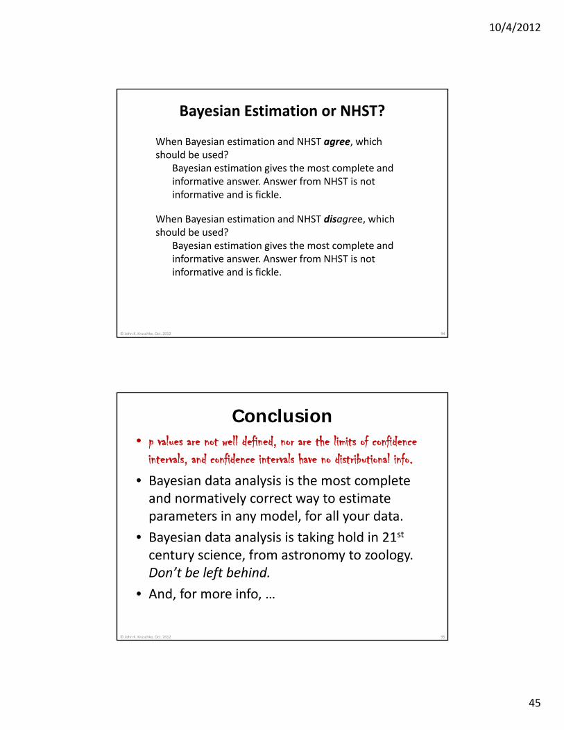
Bayesian Estimation or NHST?

When Bayesian estimation and NHST agree, which should be used?

Bayesian estimation gives the most complete and informative answer. Answer from NHST is not informative and is fickle.

94

When Bayesian estimation and NHST disagree, which should be used?

Bayesian estimation gives the most complete and informative answer. Answer from NHST is not informative and is fickle.

Conclusion• p values are not well defined, nor are the limits of confidence

intervals, and confidence intervals have no distributional info.

• Bayesian data analysis is the most complete and normatively correct way to estimate parameters in any model, for all your data.

• Bayesian data analysis is taking hold in 21st

century science, from astronomy to zoology. Don’t be left behind.

• And, for more info, …


10/4/2012

46


The blog: http://doingbayesiandataanalysis.blogspot.com/

Kruschke, J. K. (2011). Doing Bayesian Data Analysis: A Tutorial with R and BUGS.Academic Press / Elsevier.

Kruschke, J. K. (2010). What to believe: Bayesian methods for data analysis. Trends in Cognitive Sciences, 14(7), 293-300.

Kruschke, J. K. (2010). Bayesian data analysis. Wiley Interdisciplinary Reviews: Cognitive Science, 1(5), 658-676.

Kruschke, J. K. (2011). Bayesian assessment of null values via parameter estimation and model comparison. Perspectives on Psychological Science, 6(3), 299-312.

Kruschke, J. K. (2012). Bayesian estimation supersedes the t test. Journal of Experimental Psychology: General.


Program and manuscript athttp://www.indiana.edu/~kruschke/BEST/

80 90 100 110 120 130

0.0

0.2

0.4


y

p(y)

N1 = 47

80 90 100 110 120 130

0.0

0.2

0.4


y

p(y)

N2 = 42

Normality

log10(ν)0.0 0.2 0.4 0.6 0.8

mode = 0.247

95% HDI0.0486 0.464

Group 1 Mean

μ1100 101 102 103

mean = 102

95% HDI101 102

Group 2 Mean

μ2100 101 102 103

mean = 101

95% HDI100 101

Difference of Means

μ1 − μ2−1 0 1 2 3

mean = 1.021.1% < 0 < 98.9%

95% HDI0.17 1.89

Group 1 Std. Dev.

σ1

1 2 3 4 5

mode = 1.98

95% HDI1.28 2.95

Group 2 Std. Dev.

σ2

1 2 3 4 5

mode = 0.997

95% HDI0.672 1.47


σ1 − σ2

0 1 2 3

mode = 0.8920.5% < 0 < 99.5%

95% HDI0.164 1.88

Effect Size

(μ1 − μ2) (σ12 + σ2

2) 2

−0.5 0.0 0.5 1.0 1.5 2.0

mode = 0.6381.1% < 0 < 98.9%

95% HDI0.0696 1.23

80 90 100 110 120 130

0.00.2

0.4


y

p(y) N1 = 47

80 90 100 110 120 130

0.00.2

0.4


y

p(y) N2 = 42

Normality

log10(ν)0.0 0.2 0.4 0.6 0.8

mode = 0.247

95% HDI0.0486 0.464

Group 1 Mean

μ1100 101 102 103

mean = 102

95% HDI101 102

Group 2 Mean

μ2100 101 102 103

mean = 101

95% HDI100 101

Difference of Means

μ1 − μ2−1 0 1 2 3

mean = 1.021.1% < 0 < 98.9%

95% HDI0.17 1.89

Group 1 Std. Dev.

σ1

1 2 3 4 5

mode = 1.98

95% HDI1.28 2.95

Group 2 Std. Dev.

σ2

1 2 3 4 5

mode = 0.997

95% HDI0.672 1.47


σ1 − σ2

0 1 2 3

mode = 0.8920.5% < 0 < 99.5%

95% HDI0.164 1.88

Effect Size

(μ1 − μ2) (σ12 + σ2

2) 2

−0.5 0.0 0.5 1.0 1.5 2.0

mode = 0.6381.1% < 0 < 98.9%

95% HDI0.0696 1.23

80 90 100 110 120 130

0.00.2

0.4


y

p(y)

N1 = 47

80 90 100 110 120 130

0.00.2

0.4


y

p(y)

N2 = 42

Normality

log10(ν)0.0 0.2 0.4 0.6 0.8

mode = 0.247

95% HDI0.0486 0.464

Group 1 Mean

μ1100 101 102 103

mean = 102

95% HDI101 102

Group 2 Mean

μ2100 101 102 103

mean = 101

95% HDI100 101

Difference of Means

μ1 − μ2−1 0 1 2 3

mean = 1.021.1% < 0 < 98.9%

95% HDI0.17 1.89

Group 1 Std. Dev.

σ1

1 2 3 4 5

mode = 1.98

95% HDI1.28 2.95

Group 2 Std. Dev.

σ2

1 2 3 4 5

mode = 0.997

95% HDI0.672 1.47


σ1 − σ2

0 1 2 3

mode = 0.8920.5% < 0 < 99.5%

95% HDI0.164 1.88

Effect Size

(μ1 − μ2) (σ12 + σ2

2) 2

−0.5 0.0 0.5 1.0 1.5 2.0

mode = 0.6381.1% < 0 < 98.9%

95% HDI0.0696 1.23

97

10/4/2012

47

Priors are not capricious1. Priors are explicitly specified and must be acceptable to a

skeptical scientific audience.2. Typically, priors are set to be noncommittal and have very

little influence on the posterior.3. Priors can be informed by well‐established data and theory,

thereby giving inferential leverage to small samples.4. When there is disagreement about the prior, then the

influence of the prior on the posterior can be, and is, directly investigated. Different theoretically‐informed priors can be checked.

5. Not using priors can be a serious blunder! E.g., drug/disease testing without incorporating prior knowledge of base rates.


Prior credibility is not intentions

Bayesian PriorNHST Intention (e.g., stopping rule,

number of comparisons)

Explicit and supported by previous data. Unknowable

Should influence interpretation of data.

Should not influence interpretation of data


10/4/2012

48


http://doingbayesiandataanalysis.blogspot.com/2011/10/bayesian‐models‐of‐mind‐psychometric.html

100


Bayesian estimation or Bayesian model comparison?

Bayesian estimation is also better than the “Bayesian t test,” which uses the “Bayes factor” from Bayesian model comparison…

Kruschke, J. K. (2011). Bayesian assessment of null values via parameter estimation and model comparison. Perspectives on Psychological Science, 6(3), 299‐312.

Chapter 12 of Kruschke, J. K. (2011). Doing Bayesian Data Analysis: A

Tutorial with R and BUGS. Academic Press / Elsevier.

101

Kruschke, J. K. (in press). Bayesian estimation supersedes the t test. Journal of Experimental Psychology: General.Appendix D.

Doing Bayesian Data Analysis · 10/4/2012 2 Bayesian Reasoning The role of data is to re-allocate...

Documents

Transcript of Doing Bayesian Data Analysis · 10/4/2012 2 Bayesian Reasoning The role of data is to re-allocate...