Does the Basel III countercyclical capital buffer mitigate ...Kruger+Libertucci+Slides.pdfx dampen...

Does the Basel III countercyclical capital buffer mitigate regulatory capital (pro)cyclicality?

Evidence from empirical tests

- preliminary and incomplete

Massimo Libertucci

Banca d’Italia

joint work with Ulrich Krüger (Deutsche Bundesbank)

EBA Policy Research Workshop London, 14 November 2013

Disclaimer

The opinions expressed are those of the authors and do not necessarily reflect those of Bank of Italy and Deutsche Bundesbank

Outline

1. Introduction

– Motivation and main results

2. Stylized facts for financial cycles in Germany and Italy

3. Empirical estimation of firms´ probabilities of default

– Empirical estimations of PDs

– Data

4. CCB and procyclicality: an empirical test

– Methodology

– Results

5. Extensions

6. Conclusions and policy implications

4

Introduction 1/3

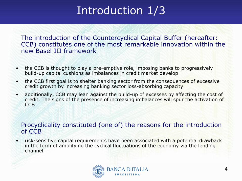
The introduction of the Countercyclical Capital Buffer (hereafter: CCB) constitutes one of the most remarkable innovation within the new Basel III framework

• the CCB is thought to play a pre-emptive role, imposing banks to progressively build-up capital cushions as imbalances in credit market develop

• the CCB first goal is to shelter banking sector from the consequences of excessive credit growth by increasing banking sector loss-absorbing capacity

• additionally, CCB may lean against the build-up of excesses by affecting the cost of credit. The signs of the presence of increasing imbalances will spur the activation of CCB

Procyclicality constituted (one of) the reasons for the introduction of CCB

• risk-sensitive capital requirements have been associated with a potential drawback in the form of amplifying the cyclical fluctuations of the economy via the lending channel

5

Introduction 2/3

The 2009 consultative document issued by Basel Committee for Banking Supervision (BCBS 2009) delineated – inter alia - a complete toolkit to tackle procyclicality…

BCBS 2009 proposal initially incorporated 4 different instruments, each of one aimed at a different policy target.

√ conserve capital to build buffers that can be used in stress

√ achieve the broader macro-prudential goal of protecting the banking sector from periods of excess credit growth

x dampen any excess cyclicality of the minimum capital requirement

√ the fourth issue of provisions has been addressed by the Accounting world; thus to some extent it lies behind the cycle of banking supervision

The first 2 objects have experienced a follow up within the final draft of the Basel III framework in the form of 2 policy instruments:

• the capital conservation buffer and the countercyclical capital buffer respectively

6

Introduction 3/3

Conversely, the proposal initially included in the BCBS (2009) consultative paper to directly tackle excessive cyclicality of capital requirements has known a different fate

• BCBC (2009) referred to some specific proposals already put forward in the reform debate (e.g. CEBS 2009 Pillar 2 or UK FSA 2009 non-cyclical PDs)

• core of these proposals: an additional capital buffer deriving from the introduction of a bank-specific mechanism that accounts for the historical performance of the PDs during the cycle

7

Motivation and main results 1/3

In spite of all potential gains, a micro-based anti-cyclical tool has been left out the final draft of the proposal

• appetite of the regulatory community for avoiding a proliferation of new risk measures potentially prone to the same form of fallacy of composition already existing

Commentators have started to shed doubts on the real ability of the anticyclical toolkit in its final design to achieve all its targets

• Enria and Quagliariello (2010) stress the importance of introducing a micro-perspective (in their definition, represented by PD-smoothing alike proposals) into the macro-prudential toolkit

• Repullo and Saurina (2011) argue that the CCB may end up by exacerbating the inherent pro-cyclical nature of the Basel framework, rather than reducing it

8


The need to further evaluate the actual anti-cyclical potential of the CCB motivates this paper

• we follow Repullo, Saurina, and Trucharte, 2010

• we test whether CCB can achieve a secondary policy goal

• we assess CCB performance with respect to some of the leading alternative procedures that have been proposed to mitigate the excess cyclicality issue

• we do so minimizing the deviations of each adjusted series with respect to a benchmark, in the form of a filtered version of the original capital requirement series

9


Preliminary results show that, under the hypotheses of this study, the CCB performs poorly in tackling excessive volatility of capital requirement

• more limited potential whether compared to other options, as a correction factor based on business cycle variables (e.g. GDP growth)

We refrain assessing the ability of CCB to achieve its primary broader goal of protecting the banking sector from periods of excess credit growth

• a suitable design of CCB can make this job (Drehmann and Juselius, 2013)

• some insights of this work may contribute to inform the current debate on implementation of CCB (e.g. ESRB role under CRD IV)

10

Stylized facts for financial cycles in DE and IT 1/3

To better comprehend the functioning of the CCB, the anatomy of the financial cycle represents the natural starting point (Drehmann et al. (2010), Arnold et al. (2012)): three sets of stylized facts

• the behavior of private sector credit and property prices provides the best description of financial cycle. On the contrary, equity bubble bursts represent a mere hiccup in the longer financial cycle

• the peak of financial cycle tends to coincide with episodes of severe financial distress; conversely, in few episodes these peaks do not end up with a crisis

• the basis of the previous two sets is it possible to build up a series of early warning indicators of financial crisis. These indictors hinge on private credit and property prices

11


The final design of the CCB (BCBS 2010) fully incorporates the above three facts

• The deviation credit-to-GDP gap represents the preferred reference variable for the build-up phase (BCBS). The use of a deviation from a medium-term trend is consistent with the theoretical facts depicted above.

A graphical inspection of this variable time series represents a starting point for the analysis

12


Some insights drawn from graphical inspection

• Type I and Type II errors: starting from the two charts, highlight how the Gap was able to identify some crisis phenomena (e.g. Italy 2008) but missing other (Germany 2008)

• Signal of overheating issued (high Gap) even after the explosion of the 2008 crisis in Italy

The relation between the credit-to-GDP ratio gap and the business cycle represents a major concern

• financial cycle is neither necessarily nor normally in synch with the business cycle

• correlation analysis tend to confirm it: negative correlation coefficients

this may cause risk of building up buffer in recessionary periods (Repullo et al. 2011)

13

Empirical estimation of PDs 1/2

The core of our analysis aims at evaluating the effects of the interaction of the CCB with some Basel II-alike capital requirements

• an adequately long time series of risk sensitive bank capital requirements represents the necessary input of the analysis

We estimate models of default probability to use as inputs to calculate capital requirements

• we use available information to compute how the capital requirements would have been evolved over time if Basel II had been in order

• admittedly, this approach represents a second-best solution, prone to Lucas´critique

• nevertheless, this procedure shows some desirable features (Kashyap and Stein (2004), Saurina and Trucharte (2007); and CEBS 2009)

14

Empirical estimation of PDs 2/2

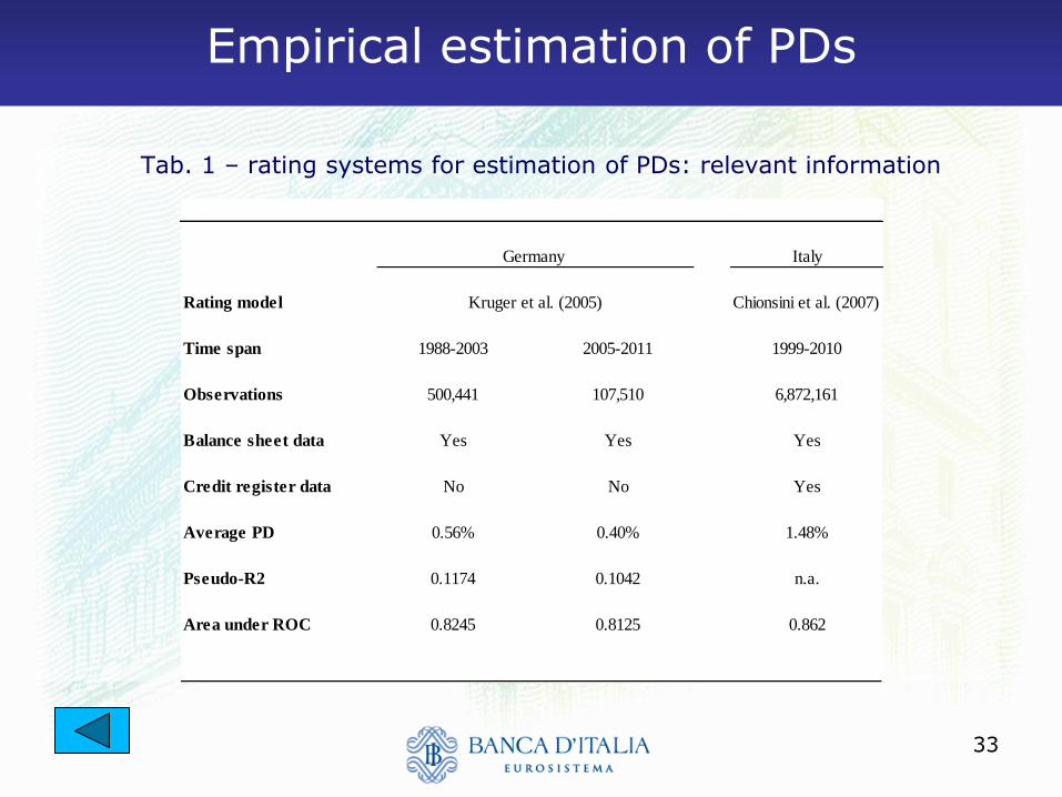
We use two different rating models for German and Italian firms

• for German firms, we use the model developed by Krüger, Stötzel and Trück (2005)

• for Italian firms, we use the rating model developed by Chionsini, Fabi and Laviola (2007)

Data sources: Germany

• information from a database of annual balance sheet information of non-financial enterprises to classify trade-bills of companies as eligible collateral for the use in refinancing operations.

• data quality issues and structural break (2003) led to the decision to split into in two sub-samples: 1988-2001 and 2005-2011

Data source: Italy

• the Italian Central Credit Register: credit information record for all the credit transactions with a value above EUR 35,000. The Register contains all the relevant information related with the characteristic of a given loan

Table 1 shows most relevant information

15

CCB and procyclicality: an empirical test 1/12

Methodology

• starting from the above PDs, we work out the corresponding Basel II Point-In-Time (PIT) IRB capital requirement for each borrower in the sample for a given year, assuming Basel II had been in place

• we use the F-IRB corporate regulatory formula

• we then calculate the annual averages

Average PIT capital requirements are negatively correlated with

GDP growth in both countries

• the cyclical behavior of risk-sensitive metric implies a significant degree of dispersion of the capital requirements

16


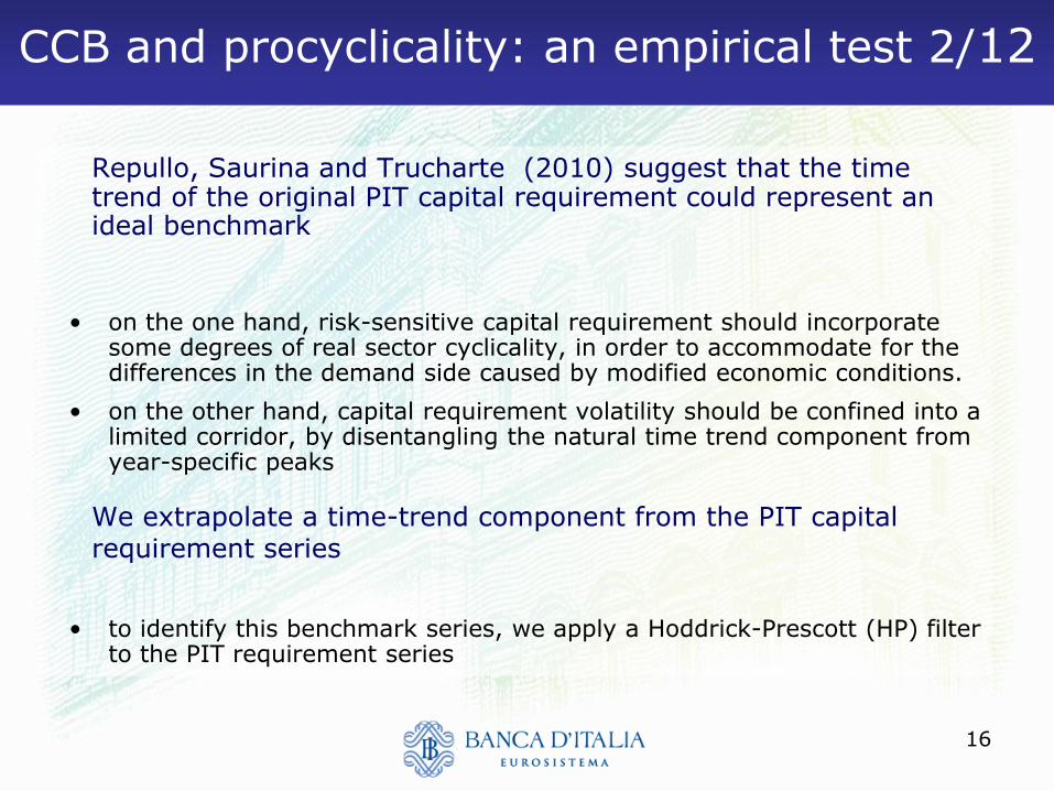
Repullo, Saurina and Trucharte (2010) suggest that the time trend of the original PIT capital requirement could represent an ideal benchmark

• on the one hand, risk-sensitive capital requirement should incorporate some degrees of real sector cyclicality, in order to accommodate for the differences in the demand side caused by modified economic conditions.

• on the other hand, capital requirement volatility should be confined into a limited corridor, by disentangling the natural time trend component from year-specific peaks

We extrapolate a time-trend component from the PIT capital requirement series

• to identify this benchmark series, we apply a Hoddrick-Prescott (HP) filter to the PIT requirement series

17


Fig 2.a – average PIT capital requirement and benchmark time trend: Germany 1998-2001

.02

8.0

3.0

32

.03

4.0

36

1988 1990 1992 1994 1996 1998 2000Year

PIT capital requirement Capital requirement HP trend

Note: This figure shows the PIT capital requirement for a one unit EAD for German corporate (solid line) together with its HP-trend (dashed line) Source: Authors´calculation

Figure 3.a - Germany 1988-2001

18


Average PIT capital requirement and benchmark time trend: Germany 2005-11 and Italy 1999-2010

.02

7.0

28

.02

9.0

3.0

31

.03

2

2005 2007 2009 2011Year


Note: This figure shows the PIT capital requirement for a one unit EAD for German corporate (solid line) together with its HP-trend (dashed line) Source: Authors´calculation

Figure 3.b - Germany 2005-2011

.04

.04

5.0

5.0

55

1999 2001 2003 2005 2007 2009 2011Year


Note: This figure shows the PIT capital requirement for a one unit EAD for Italian corporate (solid line) together with its HP-trend (dashed line) Source: Authors´calculation

Figure 3.c - Italy

19


In turn, we use the HP-filtered series as a benchmark to assess our options

How do we assess volatility reduction performance?

i. for a given Country, we are given both a PIT capital requirement series and its HP time trend

ii. we can calculate the distance between the two series: this distance is captured by the root means square deviation (RMSD) value

iii. then, we use one of the options presented in the following slide to adjust the PIT series

iv. even for this new series, we can calculate the distance from the benchmark

v. if we consider the HP trend as the “ideal” capital requirements series, we will award a good performance if, thanks to the adjustment, the distance from this ideal benchmark is reduced

20


21


22


Fig. 3 – Performance of different adjustment options: a graphical example

.02

8.0

3.0

32

.03

4.0

36

1988 1990 1992 1994 1996 1998 2000Year


Adjusted capital requirement: GDP growth

Note: This figure shows the PIT capital requirement for a one unit EAD for German corporate (solid line) together with its adjustment using a multiplier based on GDP growth (dotted line) and its HP-trend (dashed line) Source: Authors´calculation

Figure 5.a - Germany 1988-2001

23


Tab. 2 – Performance of core adjustment options

Adjustment options α RMSD Perfomance

Germany 88-01 Germany 05-11 Italy 99-10 Germany 88-01 Germany 05-11 Italy 99-10 Germany 88-01 Germany 05-11 Italy 99-10

CCB textbook -- -- -- 0.0051 0.0008 0.0061 363.7% 0.0% 124.1%

CCB lag -- -- -- 0.0048 0.0008 0.0036 329.1% 0.0% 32.8%

CCB textbook discretion -- -- -- -- 0.0008 0.0029 -- 0.0% 7.6%

CCB lag discretion -- -- -- -- 0.0008 0.0030 -- 0.0% 9.5%

GDP growth 0.0288 0.0297 0.0359 0.0008561 0.0004 0.0023 -22.7% -49.0% -15.8%

GDP growth positive 0.0276 0.0223 0.0350 0.0009 0.0006 0.0024 -18.5% -23.0% -12.3%

This table reports the perfomance of several adjustment options. Performance is calulated as variation of the root mean square deviation (RMSD) of the adjusted capital requirement

series from the Hodrick-Prescott (HP) trend of the relevant original PIT one.

A negative (positive) performance value signals a less (more) cyclical capital requirements. a is a Maximum Likelihood estimated parameter that minimises the RMSD of the adjusted

series. The notation "--" stands for a non relevant scenario.

24


Tab. 3 – Performance of other adjustment options



Credit growth 0.0060 0.0126 0.0535 0.0011 0.0009 0.0020 -0.8% 16.9% -27.6%

Credit growth positive 0.0051 0.013 0.0580 0.0011015 0.0008 0.0022 -0.6% 158.0% -19.3%

House -0.005 0.015 0.0109 0.001 0.001 0.003 -0.7% -8.5% -1.3%

Stock market -0.013 0.004 0.0177 0.001 0.001 0.003 -2.0% -0.5% -3.2%

TTC -- -- -- 0.0009 0.0014 0.0025 -20.4% 82.7% -8.0%


series from the Hodrick-Prescott (HP) trend of the relevant original PIT one.


series. The notation "--" stands for a non relevant scenario.

25


Results

• CCB does not seems fit for reducing capital requirement volatility

– a (n unlikely) purely mechanical implementation provides the lowest performance

– allowing for variations improves performance

• Using business cycle correction based on GDP growth allows for better results…

– … even in a “asymmetric implementation” that consider only above-the-average adjustments

• GDP growth outperforms credit/property prices growth performances

26

Extensions 1/2

Time-varying LGD

• so far, assumed constant LGD=45%

• however banks can also estimate their own LGD. In turn, this may cause an additional source of pro-cyclicality

• business cycle adjustments perform well also in this setting

Through-The-Cycle (TTC) PD

• acting on the inputs of the regulatory formula (“smoothing the input”)

• three-year rolling average of PIT PD

• good performance, in line with GDP growth

Further possible extensions

• the role of voluntary buffers /target ratio

• hierarchy of policy goals for the CCB

• ability to lean against the credit cycle

27

Extensions 2/2

Tab. 3 – Performance of adjustment options with time-varying LGD



GDP growth 0.006 0.025 -0.056 0.002 0.001 0.008 -15.8% -28.4% -6.7%

Credit growth 0.008 -0.022 0.098 0.002 0.002 0.004 11.7% -4.1% -16.6%

House -0.014 0.036 0.026 0.002 0.002 0.006 2.8% -9.0% -1.4%

Stock market 0.012 0.005 0.047 0.002 0.002 0.005 -58.6% -0.2% -4.0%


series from the Hodrick-Prescott (HP) trend of the time-varying LGD PIT one.


series.

28

Conclusion 1/2

Following Repullo, Saurina and Trucharte (2010) we assess the

performance of CCB, as well as other different proposals, in tackling excessive cyclicality of risk sensitive capital requirements for two samples of German and Italian firms over a combined period 1988-2011

• results are preliminary, thus caution is needed

• nevertheless, preliminary results seem to show CCB seems unfit to achieve the goal of tackling excessive cyclicality of capital requirements. In the proposed framework, CCB tend to amplify the distance from the ideal benchmark

• with respect to a purely mechanical (unrealistic) implementation of the CCB, the performance of this instrument can be improved if:

– i) a sensitive phasing-in is proposed; and

– ii) we assume some form of sensitive discretion that allowed to pull down CCB during recessionary periods

29

Conclusion 2/2

These preliminary results seem to be in line with concerns

expressed by other commentators

• CCB seems not respect Hippocratic rule “First, do not harm” (Repullo et al. 2011)

• final version of Basel III anti-cyclical toolkit is incomplete and lacking of an appropriate micro-perspective (Enria and Quagliariello, 2010)

Other adjustment procedures seem to perform better

• in particular, simple, smoothing-the-output alike proposal based on GDP growth seems to provide the best performance under the proposed approach

These results must be read together with the ability of CCB to achieve its primary goal of protecting the banking sector from periods of excess credit growth

• this analysis goes behind the scope of this work; more investigation on eventual unintended consequences of this tool is needed

THANK YOU

Massimo Libertucci

[email protected]

mailto:[email protected]

31


60

80

100

120

tren

d_

recu

rs

60

80

100

120

Cre

dit-t

o-G

DP

ratio

1970 1975 1980 1985 1990 1995 2000 2005 2010Time Name

Note: This figure shows the credit-to-GDP ratio for Germany (LHS, solid line) together with its one-side recursive HP trend (RHS, dashed line). Pale shaded areas represent periods when the HP gap was greater than 2. Dark shaded areas represent period of GDP growth below -0.5 percent. Source: the World Bank, Authors´calculation

Figure 1.a - Germany

40

60

80

100

120

HP

tre

nd

40

60

80

100

120

Cre

dit-t

o-G

DP

ratio

1970 1975 1980 1985 1990 1995 2000 2005 2010Year

Note: This figure shows the credit-to-GDP ratio for Italy (LHS, solid line) together with its HP trend (RHS, dashed line). Pale shaded areas represent periods when the HP gap was greater than 2. Dark shaded areas represent period of GDP growth below -0.5 percent. Source: the World Bank, Authors´calculation

Figure 1.b - Italy

32

Stylized facts for financial cycles in DE and IT

Ktot

Kpit

CCB

0 %

2.5 %

8 %

10.5 %

t

t

Financ

ial cycle

Busine

ss cycle

Ktot

kpit

CCB

0 %

2.5 %

8 %

10.5 %

t

t

Finan

cial

cycle

Busin

ess

cycle

33

Empirical estimation of PDs

Tab. 1 – rating systems for estimation of PDs: relevant information

Italy

Rating model Chionsini et al. (2007)

Time span 1988-2003 2005-2011 1999-2010

Observations 500,441 107,510 6,872,161

Balance sheet data Yes Yes Yes

Credit register data No No Yes

Average PD 0.56% 0.40% 1.48%

Pseudo-R2 0.1174 0.1042 n.a.

Area under ROC 0.8245 0.8125 0.862

Germany

Kruger et al. (2005)

Does the Basel III countercyclical capital buffer mitigate ...Kruger+Libertucci+Slides.pdfx dampen...

Documents

Transcript of Does the Basel III countercyclical capital buffer mitigate ...Kruger+Libertucci+Slides.pdfx dampen...